Generalized Variational Principles, Global Weak Solutions and …weinan/s... · 2006-12-15 ·...
32
Commun. Math. Phys. 177, 349 380 (1996) Communications IΠ Mathematical Physics © Springer Verlag 1996 Generalized Variational Principles, Global Weak Solutions and Behavior with Random Initial Data for Systems of Conservation Laws Arising in Adhesion Particle Dynamics Weinan E 1 , Yu.G. Rykov 2 , Ya.G. Sinai 3 1 Courant Institute of Mathematical Sciences, New York, NY 10012, USA 2 Keldysh Institute of Applied Mathematics of Russian Academy of Sciences, Moscow, Russia 3 Mathematics Department, Princeton University, Princeton, NJ 08544, USA and Landau Institute of Theoretical Physics, Moscow, Russia Received: 30 December 1994/in revised form: 1 May 1995 Abstract: We study systems of conservation laws arising in two models of adhesion particle dynamics. The first is the system of free particles which stick under colli sion. The second is a system of gravitationally interacting particles which also stick under collision. In both cases, mass and momentum are conserved at the collisions, so the dynamics is described by 2 x 2 systems of conservations laws. We show that for these systems, global weak solutions can be constructed explicitly using the initial data by a procedure analogous to the Lax Oleinik variational principle for scalar conservation laws. However, this weak solution is not unique among weak solutions satisfying the standard entropy condition. We also study a modified grav itational model in which, instead of momentum, some other weighted velocity is conserved at collisions. For this model, we prove both existence and uniqueness of global weak solutions. We then study the qualitative behavior of the solutions with random initial data. We show that for continuous but nowhere differentiable random initial velocities, all masses immediately concentrate on points even though they were continuously distributed initially, and the set of shock locations is dense. 1. Introduction This paper has two main goals: The first is to give an explicit construction of weak solutions for the initial value problem of the systems of conservation laws: :°o and f (pu) x = 0 (pu 2 ) x = pg x (1.2) 9χχ = P The second is to study the qualitative behavior of such weak solutions when initial data are random. We prove that for a wide class of probability distributions for the
Transcript of Generalized Variational Principles, Global Weak Solutions and …weinan/s... · 2006-12-15 ·...

Commun. Math. Phys. 177, 349 - 380 (1996) Communications IΠ
MathematicalPhysics
© Springer-Verlag 1996
Generalized Variational Principles, GlobalWeak Solutions and Behavior with RandomInitial Data for Systems of Conservation LawsArising in Adhesion Particle Dynamics
Weinan E 1, Yu.G. Rykov2, Ya.G. Sinai3
1 Courant Institute of Mathematical Sciences, New York, NY 10012, USA2 Keldysh Institute of Applied Mathematics of Russian Academy of Sciences, Moscow, Russia3 Mathematics Department, Princeton University, Princeton, NJ 08544, USA and Landau Instituteof Theoretical Physics, Moscow, Russia
Received: 30 December 1994/in revised form: 1 May 1995
Abstract: We study systems of conservation laws arising in two models of adhesionparticle dynamics. The first is the system of free particles which stick under colli-sion. The second is a system of gravitationally interacting particles which also stickunder collision. In both cases, mass and momentum are conserved at the collisions,so the dynamics is described by 2 x 2 systems of conservations laws. We showthat for these systems, global weak solutions can be constructed explicitly using theinitial data by a procedure analogous to the Lax-Oleinik variational principle forscalar conservation laws. However, this weak solution is not unique among weaksolutions satisfying the standard entropy condition. We also study a modified grav-itational model in which, instead of momentum, some other weighted velocity isconserved at collisions. For this model, we prove both existence and uniquenessof global weak solutions. We then study the qualitative behavior of the solutionswith random initial data. We show that for continuous but nowhere differentiablerandom initial velocities, all masses immediately concentrate on points even thoughthey were continuously distributed initially, and the set of shock locations is dense.
1. Introduction
This paper has two main goals: The first is to give an explicit construction of weaksolutions for the initial value problem of the systems of conservation laws:
: ° oand
f (pu)x = 0(pu2)x = -pgx (1.2)
9χχ = P
The second is to study the qualitative behavior of such weak solutions when initialdata are random. We prove that for a wide class of probability distributions for the

350 W. E, Yu.G. Rykov, Ya.G. Sinai
initial data, almost every weak solution has the following structure: At any positivetime t > 0, p( , t) becomes a purely singular measure even though it may becontinuous at t = 0. Moreover, this singular measure is supported on a dense setwhich can also be considered as the shock set of u. We will also study a variantof (1.2) in which a weighted velocity instead of momentum is conserved at thecollisions [GMS, VFDN]:
= 0
Our construction of weak solutions for (1.1) is based on a connection between(1.1) and the "sticky particle model" of Zeldovich (see [Z] and also [CPY]). There isa similar connection between (1.2) and the gravitationally interacting sticky particles.Consider a system of particles on Rι with initial velocities {vj}, locations {x?} andmasses {rrή}, j G Z. The particles move with constant velocities unless they collide.At collisions the colliding particles stick and form a new massive particle. The massand velocity of this new particle are given by the laws of conservation of mass andmomentum. This model was proposed by Zeldovich [SZ], and developed furtherby Kofman, Shandarin, et al. (see [GMS,KPS], and the survey paper [VDFN]) toexplain the formation of large scale structures in the universe. In this context itis also referred to as the model of "adhesion dynamics." One main result of thispaper is that the adhesion dynamics of free particles is in a sense integrable, andthis gives rise to weak solutions of (1.1).
A similar connection exists between (1.2) and the gravitationally interactingsticky particles. The Hamiltonian governing the dynamics between collisions isgiven by 2
H(p,x) = Σ p~ + Σ mmj\xi - xj\ . (1.4)
We will assume that Σ / mι < °° When particles collide, again they form a newparticle with mass and velocity given by the conservation of mass and momentum.The gravitational force acting on a particle is proportional to the difference betweenthe total masses from the right and from the left of the particle. This system is alsointegrable in the same sense and leads to weak solutions of (1.2).
For smooth solutions, (1.1) is equivalent to the Burgers equation
j)=0 ( L 5 )
together with a scalar transport equation
= 0. (1.6)
Given the initial data {po9 o}> the solution of (1.5)—(1.6) can be easily found viathe method of characteristics. Define the forward flow map φt : Rι —» Rι by
x = Ψt(y) = y + tuo(y). (1.7)
For small t, this map is usually invertible, and we have
, - 1t (x)), p(xj) = po(
where y = φ^ι(x) defines the backward flow map.
dx~X
dy(1.8)

Conservation Laws in Adhesion Particle Dynamics 351
It is well-known [L] that this construction ceases to be valid after some criti-cal time Γ* at which the solution of (1.5) develops shocks. In general (1.1) and(1.5)—(1.6) also cease to be equivalent after Γ*.
In analogy with fluid mechanics, we call y the Lagrangian coordinate and φt(y)the Eulerian coordinate at time t. After Γ* the mapping y —> φt(y) is no longerone-to-one, and no longer defined by (1.7): a whole interval can be mapped to asingle point which is the location of a shock.
However, in all cases φt defines a partition ξt of Rι where elements of thepartition are given by
®(x) = {φ-ι(x), xβR1}. (1.9)
We should stress that the solutions are assumed to be continuous from the right.The elements of ξt can be either single points, or segments. More importantly,knowing ξt, we can reconstruct φt and «(•,£) from the two conservation laws:
where Ct{y) denotes the element of the partition ξt containing y9 and %(x) =φΊ~x(x). In the more general case when the initial distribution of mass is given bya nonnegative Borel measure Po, (1.10) takes the form
Both (1.10) and (1.11) state that φt(y) is now the position of the center of mass
of GOO-We are left with the key step of defining {ξt}t>o- Let us first consider the simpler
case of a finite number of particles with initial data {Xj9Vj,mj}, 1 ^ j S N. Acrucial observation is that the necessary and sufficient condition for N particles tocollide and form a single particle before, or at time t, is that
Σί=i (χj + rf)mj ^ Σ,w+i (ή + tή>\
i=\m) Σj=J+\ mj
holds for all J, 1 ^ J ^ N — 1. Indeed assume that (1.12) holds, yet there are morethan one cluster of particles at time t. Without loss of generality, let us assume thatthere are two such clusters, {1,2,...,//} and {J1 + 1,...,/V} located at X\(t) andX2{t) with Xλ(t) < X2(t). Then we have
since the conservation of mass and momentum dictates that the cluster has to belocated at the center of mass. Equation (1.13) contradicts the assumption that (1.12)holds for all j . On the other hand, assume that (1.12) is violated for some J = J\then the group of particles {I,...,/'} will never catch up with the group {Jr +1,...,/V} before time t. For details, see Sect. 3.
Before going into the continuous case, let us state the conditions we will imposeon the initial data.

352 W. E, Yu.G. Rykov, Ya.G. Sinai
Let Po, /o G M: the space of Radon measures on Rι,Po ^ 0.
(Al) Po(A) < oo for any compact A C Rι and PQ is either discrete or absolutelycontinuous with respect to the Lebesgue measure. In the latter case, we assumethat density po(x) > 0, for x G Supp(Po) If Supp^o) is unbounded, we assumeadditionally
f sdP0(s) —• + o c as \x\ —> + o o .o
(A2) The initial distribution of momentum /o is absolutely continuous with
respect to PQ. The Radon-Nikodym derivative w( , 0 ) = -^- is the initial veloc-
ity. In the case when PQ is absolutely continuous, we assume that w( ,0) is also
continuous.(A3) For any z > 0
sup |wo(*)| ^ bo(z) and lim - bo(z) = 0 .|x| z |z|-κ»Z
The first essential result of this paper is the following principle for the construc-tion of ξt using the initial data.
Generalized Variational Principle (GVP): y G Rι is the left endpoint of an ele-ment of ξt iff for any y~, y+ G Rι, such that y~ < y < y+, the following holds:
/ (η + tu(η; 0))dP0(η) f + (η + tu(η; 0))dP0(η)ι J L i l l < • L-K' r J (Λ 1 4 Λ
f d P i η ) ' ^ >
JL ill
J[y^y)dPo(η) ^
We can also formulate GVP for right endpoints of elements of ξt, but we willomit this since we do not need it.
Having {ξt}t>o, we define φt via (1.11) and the density and momentum distri-butions at time t,Pt and It, by
Pt{Δ) = P0{φγ\Δ)), It(Δ) = h{φγ\Δ)) (1.15)
for A C Rι. In the case of continuous u(x;0) the mapping φt is also continuous.It is clear that It is absolutely continuous with respect to Pt, and we can introducethe Radon-Nikodym derivative
u(x,t)=^-(x) (1.16)art
which is the velocity at (x,t).We will use the following definition of weak solutions.
Definition 1. Let (PtJt) be a family of Borel measures, weakly continuouswith respect to t, such that It is absolutely continuous with respect to Pt foreach fixed t. Define u via (1.16). (PtJt,u)t^o is a weak solution of (1.1)if for any f,g£ CQ(R1), the space of C1 -functions on Rι with compact support,and 0 < t\ < t2,
(Dl) ff(η)dPt2(η) - J f(η)dPh(η) = Jdτ f ff(η)dlτ(η) ,
(D2) Jg(η)dlί2(η) - J g(η)dlh(η) = J dτ J g\η)u(η,τ)dlτ(η) .
Conservation Laws in Adhesion Particle Dynamics 353
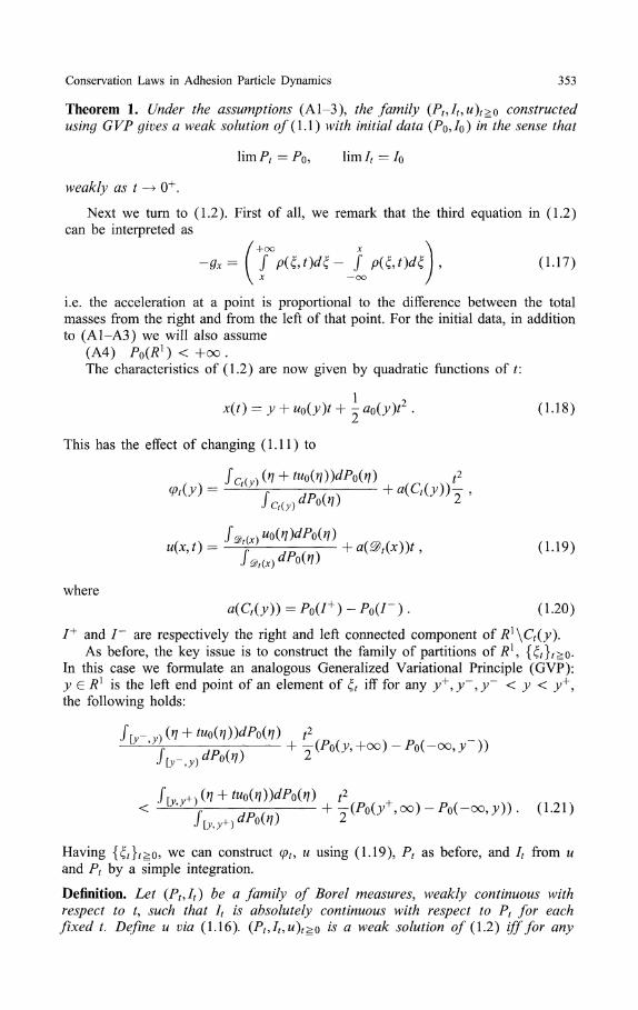
Theorem 1. Under the assumptions (Al-3), the family (Pt,It,u)t^o constructedusing GVP gives a weak solution 0/(1.1) with initial data (PoJo) in the sense that
PQ, urn/, = /o
weakly as t —> 0 + .
Next we turn to (1.2). First of all, we remark that the third equation in (1.2)can be interpreted as
( +OO X \
f p(ξ,t)dξ- f p(ξ,t)dξ)9 (1.17)/
i.e. the acceleration at a point is proportional to the difference between the totalmasses from the right and from the left of that point. For the initial data, in additionto (A1-A3) we will also assume
(A4) P0(Rι) < + o c .The characteristics of (1.2) are now given by quadratic functions of t:
x(t) = y + uo(y)t + - ao(y)t2 . (1.18)
This has the effect of changing (1.11) to
JCl(y)(η o(η))o(η) ,2Ψt{y) = — — f -=7-7 + a(Q(y))-
JΘf +a(%{x))t (1.19)
where
a(Q(y)) = Po(I+)-Po(I-). (1.20)
/ + and / " are respectively the right and left connected component of Rι\Ct(y).As before, the key issue is to construct the family of partitions of Rι
9 {ξt}t^o.In this case we formulate an analogous Generalized Variational Principle (GVP):y G Rι is the left end point of an element of ξt iff for any y+,y~,y~ < y < y+,the following holds:
/ (η + tuo(η))dPo(η) t \A Σ ^ + (P(
t
2
o o ) - P o ( - o o , 7 ) ) . (1.21)
Having {ξt}t^o, we can construct φu u using (1.19), Pt as before, and It from uand Pt by a simple integration.
Definition. Let (PtJt) be a family of Borel measures, weakly continuous withrespect to t, such that It is absolutely continuous with respect to Pt for eachfixed t. Define u via (1.16). (PtJt,u)t^o is a weak solution of (1.2) iff for any

354 W. E, Yu.G. Rykov, Ya.G. Sinai
/, g eC^R1), andO < tλ < t2,
(Dl') Jf(η)dPt2(η) - J f(η)dPtι(η) = f dτ f f'(η)dlτ(η) ,
(D2')
Jg(η)dlt2(η) - Jg(η)dlh(η) = Jdτ f g\η)u(n,τ)dlτ(η)h
+ jdτf g(η)(PM -oo) - Pτ(-oo, η))dPτ(η) .h
Theorem 2. Under the assumptions (Al-4), the family (Pt,It,u)t^o constructedusing GVP gives a weak solution of (1.2) with initial data (PQJQ) in the sense that
\\mPt = Po,
weakly as t —• 0 + .
Before continuing, let us put these results in the perspective of general hyper-bolic conservation laws. For obvious reasons, (1.1) is sometimes referred to as thepressureless gas dynamics equations. However, compared with the isentropic gasdynamics equation
= 0
(pu)t + (pu2 + p(p))x = 0
there are two important differences. First at a technical level, the natural space for(1.1) is M, the space of Radon measures, instead of BV or L°°. Secondly, thestandard entropy condition, which in the present case, takes the form
( p S ( p ) ) t + ( u p S ( p ) ) x ^ 0 , (1.23)
where S is convex, is not enough as a uniqueness criterion. Indeed in the contextof particle systems, there is a whole family of inelastic collision rules that satisfy(1.1) and (1.23). The adhesion dynamics considered here is an extreme case ofthese collision rules. It is easy to see that the weak solutions of (1.1) constructedin this paper has the additional property:
ux<\.
It is suggested by Jonathan Goodman that this might be sufficient as a uniquenesscriterion. Moreover, it is natural to expect that the adhesion dynamics correspondsto a form of viscosity limit. But this also remains to be proven. Notice that (1.1)is an extreme case of a non-strictly hyperbolic system: the two characteristic fieldscoincide.
We will also consider a model closely related to (1.2) which is also discussedin the astrophysics literature [GMS, VDFN]:
Pt + (pu)x = 0
£ ) * =-Gχ ( L 2 4 )
Qxx = P -

Conservation Laws in Adhesion Particle Dynamics 355
The relation between (1.2) and (1.24) is analogous to the relation between (1.1)and (1.5-6). Let h = gx, we can rewrite (1.24) as
Γ ht + uhx = 0
( + ( ΐ > * <i25)
If PQ is absolutely continuous, we can reduce (1.25) to a scalar conservation lawof the form
ut + (γ\ = -ho(G(x - ut, 0), (1.26)
which is amenable to standard methods. Using this, we are able to establish bothexistence and uniqueness of global weak solutions for (1.24). This is explained inSect. 6.
In the second part of this paper we study the qualitative behavior of these modelswith continuous, but non-differentiable initial data, extending some results from [S].We show that the solutions of these models share the common feature that almostsurely, at any / > 0, all masses concentrate on points (i.e. the absolute continuouspart vanishes), and the set of shock locations is dense. This behavior was to someextent anticipated by Zeldovich [Z] in his work on cosmology. In that context, thesepoint masses are interpreted as the galaxies in a one-dimensional universe.
Before ending this introduction, let us mention that. (1.1) and (1.2) also havean origin in kinetic equations. Consider
// + t>Λ = O. (1.27)
If we look for solutions of the form
f(x,υ,t) = p(x,t)δ(υ - u(x,t)), (1.28)
we obtain (1.1) for (p,u). Similarly consider the Vlasov-Poisson-Jeans equation
[VDFN]
ί ft + υfx - gxfv = 0{ r O 29)[θxx = J f(x,υ9t)dv.
If we look for solutions of the form (1.28), we obtain (1.2) for (p,u).The paper has eight sections and one appendix. In Sect. 2, we compare our
GVP with the Lax-Oleinik variational principle for scalar quasi-linear equations.In Sect. 3, we consider the discrete version of (1.1) and prove GVP for this case.In Sect. 4, we extend these results to the continuous case and complete the proofof Theorem 1. In Sect. 5, we explain the additional steps needed for the proof ofTheorem 2. In Sect. 6, we consider the modified gravitational system (1.3).
Part II consists of two sections. In Sect. 7, we consider (1.1) and (1.2) withrandom initial data. In Sect. 8, we extend these results to (1.3).
After this paper was submitted for publication, we received a preprint [BG]by Brenier and Grenier in which existence of weak solutions of (1.1) was provedwithout resorting to GVP at the continuous level. [BG] also contains some veryinteresting ideas for the multi-dimensional version of (1.1). We thank Brenier andGrenier for timely communication of their results.

356 W. E, Yu.G. Rykov, Ya.G. Sinai
Part I. Generalized Variational Principlesand Global Weak Solutions
2. Preliminaries and Comparison with the Lax-Oleinik Variational Principle
In the following we will concentrate on (1.1). The necessary changes for (1.2) willbe summarized in Sect. 5.
Intuition from adhesion dynamics suggests that the masses cluster more andmore, and the accumulated masses will never split apart again. We formulate this as:
Lemma 1. The family of partitions {ξt}t>o determined with the help of GVP isdecreasing. In other words, for 0 < t' < t, each element of ξt is contained in anelement of ξtt.
Proof Assume to the contrary that there exists y G dζt, but y£dξt*9 where dξt
denotes the collection of points belonging to the boundary of some element of ξt.Without loss of generality, we can assume that y is the left end point of an elementin ξt. Then for some y~ < y < jμ+, we should have
( ' }>
[ y , y ) = fίy,y+] dPo(
Consider two linear functions l\(s)J2(s) of s defined by
ηdPo(η)
For sufficiently small s9 we have l\(s) < I2(s) while l\(tf) ^ I2(tf). Since l\ andl2 are linear, we conclude that l\{t) > I2(t). This contradicts the fact that y e dξt:i.e. y satisfies GVP at time t.
Now we will compare GVP with the classical Lax-Oleinik variational principlesee [L, O]. We assume that PQ has a density po> a n d 0 < const ^ PoOO < oo.Introduce
y y
Φι(y) = / (η + tuo(η))po(η)dη, φ2(y) = J Po(η)dη (2.3)
and
C ( > ; ' } = 02(/') - Φ2(/) ' ( 2 ' 4 )

Conservation Laws in Adhesion Particle Dynamics 357
02 defines a C^-diffeomorphism of/?1. Let y — φ^x{z)9 and define
{ ^ ) ι _ r ( )
In these notations, (1.14) becomes
inf c(y,y+) ^ sup c(y~,y) (2.6)y+>y y-<y
or, for z = φ2(y),inf φ,z+) ^ sup φ " , z ) . (2.7)
^ + > z z-<z
Let φ(z) = φ\ o φ~ι(z). Geometrically (2.7) means that (z9φ(z)) is a point ofcontact of the graph of φ and its convex hull constructed in the coordinate z.
In comparison, the Lax-Oleinik variational principle for the Burgers equation(1.5) can be formulated as
u{x,t)=yχinϊ S^p-+ j Uo(η)dηγ (2.8)
It is easy to see that finding the minimum in- (2.8) is the same as constructingthe convex hull of the function F(y) = j y (η + tuo(η))dη and finding the points ofcontact between the graphs of F and its convex hull. In fact the set of points wherethe minimum in (2.8) is attained is exactly the same as the set of contact pointsbetween the graphs of F and its convex hull. Notice that F is a special case of φ\when po = 1 We see that the construction of GVP is the same as constructing theconvex hull, but in a special coordinate z. It is in this sense that (1.14) and (1.21)generalize the variational principle of Lax and Oleinik.
3. The Discrete Case
It is instructive to consider first the case of a finite collection of particles {(xf9 v®,m®),ί = 1,2,.. ,,N}9 where xf9 v® and m® are respectively the location, velocity, and massof the /th particle. The particles undergo adhesion dynamics, defined in Sect. 1. Theeffect of the partitions {ξt}t>o is to divide the particles into ordered groups or clus-ters G\(t),G2(t)9...,G/c(t)9 so that each group of particles are glued to a single onebefore or at time t, and different groups are at different locations at time t. If G isone such group, say G = {/,/+ l,...,y}, we denote by C G ( O its location at timet. From the conservation of mass and momentum, we know that Cc(t) has to bethe center of mass of G:
m . 0.,,More generally, we will denote the expression on the right-hand side of (3.1) byCij(t). It is a linear function of t.
Lemma 2. Let G\ and G2 be two neighboring groups of particles such thatCGι(0 < CGl(t)for t < t\ and CGι(t*) = C^t*). Then for t > t\
CGιuG2(t) < CGι(t).

358 W. E, Yu.G. Rykov, Ya.G. Sinai
Proof Since both Ccx(t) and C G 2 ( O are linear functions of t, we have for t > t*9
CGι(t) > CGl(t).
Since CG 1 UG 2 (O = otCc^t) + (1 — a)Cc2(t) for some constant α G (0,1), we havefor t > t*,
CGlUG2(t) < CGι(t).
This proves the lemma.
Lemma 3. Let G G ξt, and G = {x°, f ^ i ^ / ' } . Then for any ijr S i ^j " — 1, we have
Cj',i(t) ^ Ci+lJ,,(t). (3.2)
Proof. Assume to the contrary that there exists an ί, such that (3.2) does not hold.Since Cyjn(t) — aCfj(t) + (1 — a.)Ci+ιj»(t) for some 0 ^ α 1, we have:
C/ΛO < Cj'j»(t). (3.3)
Consider the evolution of the set of particles 7(0) = {xp f S j = 0 Each timethe set is hit from the right by a particle or a cluster of particles, we add them toour set. In this way we obtain a growing family of sets I(s) = {x®, f S j = Ks)}From Lemma 2, when new particles are added to I(s), its center of mass is movedfurther to the left, i.e.
Crj{s). (3.4)
From the assumption of the lemma we have i(t) = /''. Hence we have
Cfjn(t) <Cj,j(t), (3.5)
contradicting (3.3).
Theorem V. x^ is the left endpoίnt of an element of the partition ξt iff
max Cjt j-ι(t) < min C. Mt). (3.6)
Proof Assume that (3.6) holds, and Xj is not the left endpoint of an element of ξt.
Let G G ξt be the element of ξt containing x®, G = {xf, z'o i ύ jo} and z'o < jFrom Lemma 3, we have
C w _ , ( 0 ^ CjJo(t) . (3.7)
This clearly contradicts (3.6).Assume now that Xj is the left end point of an element of ξt. For any
/>/'> / < j < /'> w e w a n t t 0 s n o w t n a t ^/,y-i(0 < Cj,j"(t)> L e t hJiτ Ji be
the consecutive elements of & to the left of Xj, and JC°, £ I\ = {xf9 i\ ^ / ;§ z'2}
Let Jι,J2,...,Jr be the consecutive elements of ^ to the right of Xj (including the
one containing Xj), and x0,, G Jr = {xf, yΊ z 7*2}- From Lemma 3, we have
Λ 2 , Λ / φ ( 3 . 8 )
We also have
C Λ ( 0 < < C7,(0 < Cy,(ί) < < 0 , ( 0 • (3.9)
Conservation Laws in Adhesion Particle Dynamics 359
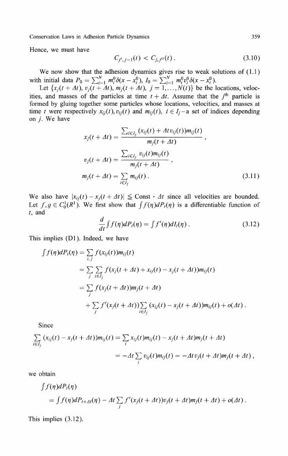
Hence, we must have
C/j-\(t) < Cjjπ(t). (3.10)
We now show that the adhesion dynamics gives rise to weak solutions of (1.1)
with initial data Po = Σ?=\ n$δ(x - *?), Io = Σ?=ι m^δ(x - x?).Let {xj(t + At), Vj(t + At), mj(t + At), 7 = 1,...,N(t)} be the locations, veloc-
ities, and masses of the particles at time t + At. Assume that the / h particle isformed by gluing together some particles whose locations, velocities, and masses attime / were respectively Xίj(t),Vij(t) and /wzy(O? * £ //-a set of indices dependingon j . We have
Xj(t + Δt) = ^ Lmj(t + At)
.o-^mj(t + At)
mjit + At) = Σ »>ij(t) > (3.H)i€lj
We also have \xij(t) — Xj(t + At)\ ^ Const At since all velocities are bounded.Let f,ge C^(Rι). We first show that ff(η)dPt(η) is a differentiable function oft, and
jtJf(η)dPt(η) = Jf'(η)dlt(η) . (3.12)
This implies (Dl). Indeed, we have
= Σ Σ f(xj(.t + Δt) + Xij(t) - xj(t + Δt))mυ(t)j i
Xij(t)-xj(t + At))mij{t) + o(At)j ieij
Since
Σ, (XijίO - xj(t + At))mij(t) = Σ XijiOmtjit) - Xj(t + Owy(ί + ^ 0/G/y /
= -Zlί Σ % ( 0 ^ ( 0 = -AtVj(t + zlί)my(ί + J
we obtain
Jf(η)dPt(η)
= Jf(η)dPt+At(η) - ΔtΣf'(Xj(t + Δt))Vj(t + Δt)mj{t + Δt) + o(Δt) .j
This implies (3.12).

360 W. E, Yu.G. Rykov, Ya.G. Sinai
In contrast Jg(η)dlt(η) is not C1 in t because of the inelastic nature ofthe collisions. To see this, consider just two particles colliding at t = τ. Be-fore collision they are denoted by {x\{t),V\{t),m\{t)),(x2(t),v2{t),m2{t)),t < τ,respectively. After collision they form a single particle (x(t),v(t),m(t)),t ^ τ.We have m(τ) = /«i(τ) + m2{τ\ m(τ)v(τ) = mχ(τ)v\(τ) + m2(τ)v2{τ\ m(τ)x(τ) =m\(τ)x\(τ) + m2(τ)x2(τ). For t < τ, we have
Jg(η)dlt(η) =
= 0(*(τ))(ι;i(O/wi(O + v2(t)m2(t))
+ (t- τ)g'(x(τ))(v\{t)mλ(t) + ^ ( 0 ^ ( 0 ) + O((ί - τ)2)
= Jg(η)dlτ(η) + (ί -
For t > τ, we have
Jg(η)dlt(η) = g{x{t))v(t)m(t)
= Jg(η)dlτ(η) + (t- τ)g'(x(τ))v2(τ)m(τ) + O((t - τ ) 2 ) .
In general, energy decreases at collisions
ι;2(τ)m!(τ) + v2
2(τ)m2(τ) + v2(τ)m(τ).
Hence Jg(η)dlt(η) is not C1 in ί. Nevertheless, we can prove that (D2) is stillvalid. We only have to prove this for the case when there is no collision in (t\,t2)and at t = t2, a group of particles, say with indices i\9 i\ + 1,..., i2, are colliding toform a single particle at x{t2). We then have
Jdτjg'{η)u{η,τ)dlτ{η) = J J i fy^W)^)™;Ί Ί '=1
'g 1
miVi±g(Xi(τ)) + j miVi±g(Xi(τ)) + J21=1 ' * dτ ι
ί = h
ι ιdτ ι
/ = / 2 + 1
A TV
Σ miVid(xi(h)) ~ Σ mivi
4. Proof of Theorem 1
We will first give the proof for the case when Po is absolutely continuous, and thenfor the case when Po is discrete.
For initial data satisfying (A1-A3), we construct a decreasing family of par-titions {ξt}t>o of Rι according to GVP (1.14). Having {6}/>o> we can defineφt,PtJt, and u(x,t). Obviously φt is a non-decreasing function of y for any fixed t.

Conservation Laws in Adhesion Particle Dynamics 361
Furthermore, as a consequence of the assumption that u(x; 0) is continuous, φt isalso continuous, and we have
Jf(η)dPt(η) = Jf(φt(η))dP0(η) ,
fg(η)dlt(η) = Jg(φt(η))dlo(η) . (4.1)
We will prove Theorem 1 via discrete approximations. Take a sequence of mea-
sures PQW) concentrated on finite sets {xf\i = 1,...,} such that P^ —> Po weakly.
Define IQ to be a signed measure concentrated on the set {x;\i — 1,...,} such
that 4n\{x\n)}) = uo(x\n))P{Q\{x\n)}). Then I™ -> 70 weakly. Using GVP, we con-
struct the corresponding families of partitions ξ^ and mappings φ^t
n\ Moreover we
already showed (Theorem 1') that for f,ge C0(Rι),
(4.2)
Here P\n\ήn) are constructed in Sect. 1. We also have for 0 < t\ < t2,
= J
J ^^\^ ^ \η,τ)dl^ . (4.3)h
We can extend the definition of φ(
t
n) to the whole line by putting φ^iy) = φ^n\x\n))
if X™ ^ y ^ χ«>l9 φ<?\y) = φ<?\χM) if y < x^\ φ<?\y) = φ<?\χ™) if y >
x%\ Here x™ = min{x^}, x%} = max{x^}}.
We will use superscript "«" to denote objects corresponding to P^J^. If Δis an interval in R *, we denote
J dP(η)
The following lemma is a continuous version of Lemma 3. It can be proven inthe same way as Lemma 3.
Lemma 3 ;. Let G — [a,b] be an element of ξt, a < b. Then for any c £ (a,b),we have
C[a,c)(t) ^ C M ] ( 0 . (4.5)
Lemma 4. φ^ —> φ uniformly on compact subsets of Rι x [0, oo).
Proof We first prove that for any fixed t ^ 0, the inverse images of φf of
a bounded interval L = (c,d) are uniformly bounded. To that end, let A^n) =
{xf°, Λ f } ) G Z } , and x^ n = min{jc<Λ), xf G A™}. Obviously x^ n has to be
the left end point of an element G ( w ) in the partition ξ^n\ From Lemma 3, we have
ZL ^zd&WZc. (4.6)

362 W. E, Yu.G. Rykov, Ya.G. Sinai
Using (A3), we can write (4.6) as
£ > c . (4.7)
Hence {x^} is uniformly bounded from below. Similarly we can prove an upperbound.
Assume to the contrary that {φt } do not converge uniformly on some boundedset, say [c,d] x [0, T], Then there exists ε > 0, and sequences {yn,tn} G [c,d] x[0, T] such that
\<P%\yn) - ΨtMl >fi (4-8)
We can choose {yn},{tn} such that l i m ^ = jμ*, limίw = t, \imcpf \yn) = x* exist.Since
Wt\yn) ~ ψΐ\yn)\ ύ |ίΛ-ί|max|w(jc;O)| ^ Const \tn-t\ (4.9)
where the maximum is taken over a bounded set, for sufficiently large n we getfrom (4.8)
\ψΐ\yn)-φt{yn)\ > \ . (4.10)
Therefore we have
|**-Φrϋ>*) | ^ | (4.11)
Without loss of generality, let us assume x* < φt(y*). Let Δn = (φ^)~x
{φ(tn\yn)} = { xf° < < Xj?} w h i c h i s a n element of ξ(
t
n\ By extracting subse-
quences, we can assume that Δn converges to an interval Δ, with Δ = [a,b], in the
sense that
l imx^ = a, limjcj^ = b . (4.12)
Consequently, we also have x* = Q ( ί ) ^ itself may be open, closed, or half-open.Since yn G Δn, we must have y* eΔ. Let ΦΓH^X^*)} = ίc>d]. By the continuityof φt9 this has to be a closed interval which might consist of a single point. Wewill discuss the case when a < b. The reader can easily see that the case whena — b also follows.
First we prove that c9de(a,b). Assume to the contrary that c G (a,b). We can
choose a sequence {x(,n)}, xf° < x(
}
n) < x{"\ such that l imx^ = c. Since x^ is
not the end point of any element in ςf , there exist y , j " , such that
d,n)
; (O^ΛίO (4.13)Jn >ιn—\ ιn,Jn
By extracting subsequences, we can further assume that {x^} and {x^)} convergeJn Jn
to c* and d*, respectively.Taking the limit of (4.13), we obtain
ffjη + t uo(η))dPo(η)
jd;dPM ' ( 4 1 4 )
contradicting (1.14). Therefore c£(a,b). Similarly d£(a,b).
Conservation Laws in Adhesion Particle Dynamics 363
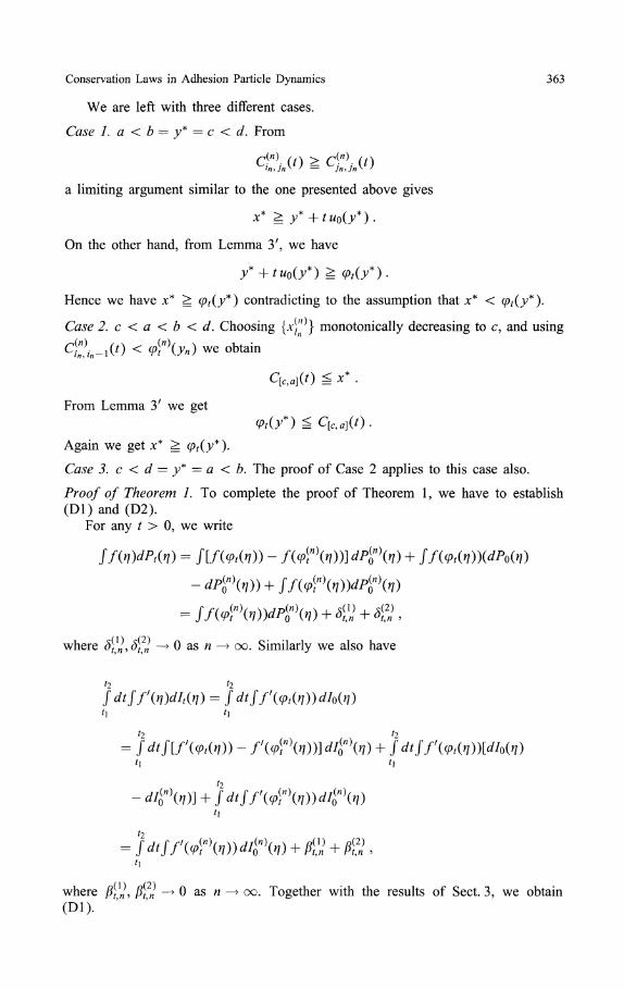
We are left with three different cases.
Case 1. a < b = y* — c < d. From
dn), (0 > cf\ (0
a limiting argument similar to the one presented above gives
x* ^ y*+tuo(y*).
On the other hand, from Lemma 3', we have
y* + tuo(y*) ^ φt(y*).
Hence we have x* ^ ψt(y*) contradicting to the assumption that x* < φt(y*).
Case 2. c < a < b < d. Choosing [x]1^} monotonically decreasing to c, and using
C/Γi-iίo < ^yn)we o b t a i n
C[c,a](t) g X*
From Lemma 37 we get
ΨtiyΊ ^ C[c,a](t).
Again we get x* ^ Φ?(j*).
Case 3. c < d — y* = a < b. The proof of Case 2 applies to this case also.
Proof of Theorem 1. To complete the proof of Theorem 1, we have to establish(Dl) and (D2).
For any t > 0, we write
Jf(η)dPt(η) = J[f(φt(η)) - f{φΐ\η))]dP^\n) + Jf(ψt(η))(dP0(η)
where ^ } W ,^ j W —> 0 as « —> oo. Similarly we also have
Jdtjf'(η)dlt(η) = }dtjf'(φt(η))dlo(η)
= }dtf[f'(φt(η)) - /'(^B)(ί/))]^B)(»/) + Jdtjf'(φt(η))[dlo(η)
= Jdtjf'iφ^md^η) + ffi + ffi ,
where βtn> Pin ~* ® a s rt "^ °° Together with the results of Sect. 3, we obtain(Dl).
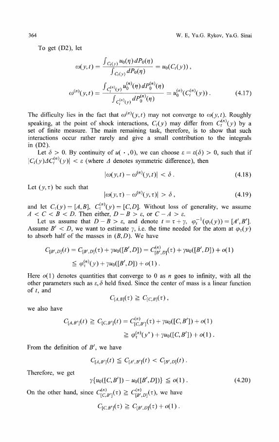
364 W. E, Yu.G. Rykov, Ya.G. Sinai
To get (D2), let
!cl(y)
dpo(n)
(4.17)
The difficulty lies in the fact that ω^n\y,t) may not converge to ω{y,t). Roughlyspeaking, at the point of shock interactions, Ct(y) may differ from C$n\y) by aset of finite measure. The main remaining task, therefore, is to show that suchinteractions occur rather rarely and give a small contribution to the integralsin (D2).
Let δ > 0. By continuity of u( ,0), we can choose ε = ε(δ) > 0, such that if
\Ct{y)ΔC(f\y)\ < ε (where A denotes symmetric difference), then
ω(y,t) - ω(n\y,t)\ < δ. (4.18)
Let (y,τ) be such that\ω(y,τ)-ω^n\y,τ)\ >δ, (4.19)
and let Cτ{y) = [A,B], c[n)(y) = [C9D]. Without loss of generality, we assumeA < C < B < D. Then either, D - B > ε, or C - A > ε.
Let us assume that D — B > ε, and denote t = τ + y, φ^ι(φt(y)) = [A\B'].Assume B' < D, we want to estimate γ, i.e. the time needed for the atom at φτ(y)to absorb half of the masses in (B,D). We have
q*',z>](τ) + yuo([B',D]) = d$tDft) + yuo([Bf,D]) + 0(1)
Here o(l) denotes quantities that converge to 0 as n goes to infinity, with all theother parameters such as ε, δ held fixed. Since the center of mass is a linear functionof t9 and
C[A,B](τ) ^ C[C,B](τ),
we also have
C[A,B'](t) ^ C[C>B/](0 = C^Bl](τ) + yuo([C,B'])
From the definition of B\ we have
q^,5;](0 = q^.^ίO < q
Therefore, we getγ{uo([C,B']) - uo([B',D])} g o ( l ) . (4.20)
On the other hand, since C^}gl](τ) ^ C ^ ^ ^ τ ) , we have

Conservation Laws in Adhesion Particle Dynamics 365
Hence, we get
Doθί) βdPo(η)
o ( l ) . (4.21)
Here β(ε) is some finite quantity depending on ε. Hence, we have
yί °4R (4-22)
Similarly, if C — A > ε, we can show that after time S-j, at least half of the
masses in (A, C) are absorbed by the atom at φ[n\y).Let S = {τ G [/i,^]? there exists j G l , L is a sufficiently large interval, such
that (4.19) holds}. Since either Po(A, C) ^ Const ε, or P0(B,D) ^ Const ε, andsince Po(L) < Const, we must have
w < I S • < 4 2 3 >Now let gGCdCR1). We choose L to contain the support of g(φτ( )),
τe[tut2l
fdτfg'iη^iηfdP^iη) - / dτfg'(η)u(η,τ)2dPτ(η)
h
/ί/τ/0'(φI(>7))[ω<")(ίy,τ)2 - © ( i j . τ ) 2 ] ^ ^ )Ί
/ί/τ/6f/((pτ(^))[ω(")(f7,τ)2 - ω(»7,τ)2]ΰίPo(/ί)
^n\η, τf - ω(η9 τ)2] dP0(η)
^ o(l) + Const \S\ + Const δ S o(l) + ^7-f + Const δ ,
where the constants depend on the support of g. Now we can choose n so large
that $$-ε+o(l) < δ. Then we get
JdτJg\η)u^\n)2dP^\η) - f dτfgf(η)u(η,τ)2dPτ(η) ^ Const δ .
Together with the argument which proved (Dl), we get (D2).
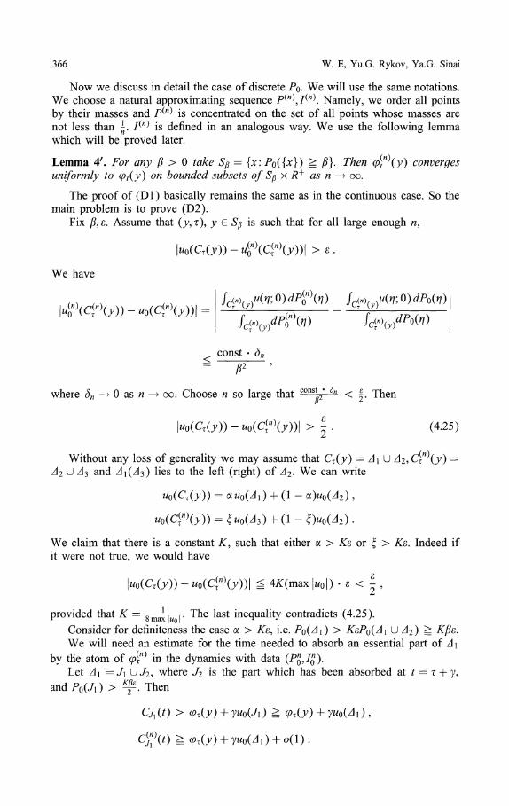
366 W. E, Yu.G. Rykov, Ya.G. Sinai
Now we discuss in detail the case of discrete Po We will use the same notations.We choose a natural approximating sequence P^n\l^n\ Namely, we order all pointsby their masses and P^ is concentrated on the set of all points whose masses arenot less than ^. 1^ is defined in an analogous way. We use the following lemmawhich will be proved later.
Lemma 4'. For any β > 0 take Sβ = {x: Po({x}) ^ β} Then φ^n\y) convergesuniformly to φt(y) on bounded subsets of Sβ x R+ as n —> oc.
The proof of (Dl) basically remains the same as in the continuous case. So themain problem is to prove (D2).
Fix j8,ε. Assume that (y,τ), y G Sβ is such that for all large enough n,
l«o(CτϋO) - u^\c[n\y))\ > ε .
We have
\n) L(n)ίMη;0)dP0(η)
const δn
β2 '
where δn -> 0 as n -> oc. Choose n so large that c o n s * 2 ' δn < | . Then
\uo(Cτ{y))-uQ{C\n\y))\ > | . (4.25)
Without any loss of generality we may assume that Cτ(y) = A\ U A2,c[n^{y) =Δ2 U Zl3 and Δ\(Ai) lies to the left (right) of Δ2. We can write
uo(Cτ(y)) =
We claim that there is a constant K, such that either oc > Kε or ξ > Kε. Indeed ifit were not true, we would have
MC t O0) - uo(C?\y))\ g 4A-(max|«o|) ε < | ,
provided that K = 8 m a ^, •. The last inequality contradicts (4.25).
Consider for definiteness the case α > Kε, i.e. Po(A\) > KεPo(Δι U Δ2) ^ X"j8β.
We will need an estimate for the time needed to absorb an essential part of A \
by the atom of φτ in the dynamics with data (PQ,/Q ).
Let A1 =J\ UJ2, where J2 is the part which has been absorbed at t = τ + y,
andPoGΛ) > ^ Then
CJχ(t) > φτ(y)

Conservation Laws in Adhesion Particle Dynamics 367
Here o( 1) means quantities which tend to zero as n —> oo and /?, ε remain fixed.We also have
o{\) .
By assumption at time ί, the set Ji is not absorbed by the atom which at time τ
were at φf , but J2 is, we can write
or
Since
we conclude
- uQ(C(
τ"\y))) ^
ε
2 '
y ^
Define Sβ = {τ e [tut2] one can find y eLΠSβ so that (4.24) holds}. As inthe continuous case, we have
Now take g e CQ(R1). We can write
h
ύ o(l) + <
4H )(>/
>2
ίl
:onst'2
\η)-Jdtfg'(η)(uτ(η))
η))[(ω(n)(ψ,τ)f-(ω(η;
I dP0(η)
2dP0(η)
τ)f]dP0(η)
Jdtjgf(φτ(η))((ω^(η;τ))2 - (ω(η;τ))2)dP0(η)
I J gf(φτ(η))(ω^\η;τ))2 -(ω(η;τ))2)dP0(η)[t{;t2]\Sβ Sβ
^ o(l) + C(β) + const 1^1 + const ε = o(l) + C(j8) + const ε .
The rest of the proof is the same as in the continuous case.
Proof of Lemma 4'. We will follow the proof of Lemma 4. Assume that one canfind a sequence {y(n)} such that P0(y(n)) ^ β and
Wt\yw) - 9,(y(n})\

368 W. E, Yu.G. Rykov, Ya.G. Sinai
for some ε > 0 and an infinite sequence of values of n. For each of these
n one can find three adjoining intervals Δ"\ n£\ A^ such that C^n){y^) =
A^ U Δ%\ Cξ(y^) = A^ U A^\ Let us assume that we have
Ψt (y^) < Ψt(y^) (4.26)
Arguing as above we conclude that either Po(A\n)) > Kλβε, or P^A^) > Kxβε
for some constant K\. For definiteness let us assume Po(Δ^) > K\βε. Then GVP
gives
CA(n)(O ^ Cjn) Λn)(t) = <Pt(y ) ^ C (n)(t) ,
or
C/n)(t) < φί(y(n)) S CUt),
Since PQ{A{^) > Kβε, PQ{Δ{^) > β, we have
This contradicts (4.26).
5. The Gravitationally Interacting Case
In this section we prove the GVP for (1.2) and Theorem 2. Since most ofthe argument is parallel to the ones in Sects. 2-4, we will only summarize thekey steps.
Lemma 5. The family of partitions {ζt}t>o is decreasing, i.e. for 0 < t' < t,dξt c dξt,
Proof. Assume to the contrary that there exists y G dξt, but y£dξ,ι. Then for somey~,y+,y~ < y < y+, we should have
J (η + t'uo(η))dPo(η) {t'
} [ y y + ]
) p o ( _ ) (

Conservation Laws in Adhesion Particle Dynamics 369
Consider two quadratic functions q\(s), q2(s) defined by
, , L-y)(η + ™0(η))dP0(η) S2
s2
+sB~ + — C ~ ,
+](η + suo(η))dPo(η) s \l 2 L A + w(poίy+, oo) - P 0 (-oo, y))
+ S-C+ .
For sufficiently small s, we have A~ < A+ and q\{s) < q2(s), while # i ( O ^ qi(t').Since C " - C + = Pol>~,.y+] > 0, A~ - A+ < 0, one of the two roots of the equa-tion #i(s) = qi(s) is negative. Since there is one positive root in (0, tf), no rootsexist in (t\oo). Therefore we have giCs1) > q2(s) for s > t\ contradicting the as-sumption that q\(ΐ) < qi(t).
There is also an obvious analog of Lemma 2 for (1.2). We omit the detailsof that.
Next we study the discrete case, using the notations of Sect. 1. In the presentsituation, the center of masses of the particles {*f,jcf+1,...,jty} becomes
Lemma 6. Let G e ξt9 G = {x?9 f ^ i ^ j"}. Then for any i, f ^ / ^ / ; - 1,we have
Cfj{t) ^ Ci+hj,,{t). (5.3)
Proof. We proceed as in the proof of Lemma 3. The key step is to show that iftwo groups of particles {(jc?,t7?,/w?), j \ ^ / ^ j} and {(*?,t;?,/w?), j + \ ύ i ύ ji}merge at time t\ then
C j ι j 2 ( s ) ^ C j u j i s ) 9 s ^ t f . (5.4)
Consider again two quadratic functions giCs1) = Cjhj(s) = A\ + B\s + C\ y , ^2(^) =
Cj+hj2(s) =A2+ B2s + C 2 y. Obviously we have ^i - A2 < 0, Ci - C2 = Σ / > ;
m ?
-Σ&jrf -Έi>j2
m? + Σi<j+ιm? = Σjιziίj2»$ > 0' Therefore the quadraticequation q\(s) — q2(s) = 0 has one negative root. Since there is already oneroot in (O,^)* there cannot be any more roots in (^,00). Therefore, wehave
CΆj(s) ^ Cj+ιj2(s% for s > t' .
This implies (5.4).

370 W. E, Yu.G. Rykov, Ya.G. Sinai
Similarly we can formulate
Theorem 1!'. Xj is the left end point of an element of ξt iff
max Cjf , _ i (0 < min C7 .-//(*). (5.5)
We now prove that the adhesion dynamics of gravitationally interacting particlesgives rise to weak solutions of (1.2). Since the proof of (Dl') is entirely the sameas the one for (Dl), we will concentrate on (D27). Again we only have to prove(D2') for the case when there is no collision in (£1, 2), and at t = h, a group ofparticles, say indexed by ΪI , . . . ,/2> collide to form the new particle at x(ti). Lethi = Σj>i mj ~ Έj<i mJ> t h e n w e h a v e
fdτfg'iηMη, τ)dlτ(η) + JdτJg(η)(Pτ(η, oo) - Pτ(-oo, τ))dPτ(η)
h h
= Jdτ Σ ^ W ^ T M + Jdτ Σ g(xM)himi
h N rf h N
= Jdτ Σ mivi(τ)-—g(xi(τ)) + JdτTV 7V
= Σ 9(Xi(t2))miVi(t2) - X)sf(^i(ίi)/=1 /=1
h N h N
- Jdτ Σ mihίg(xi(τ)) + Jdτt\ Ϊ = 1 t\ i=\
= Jg(η)dIt2(η)-Jg(η)dItι(η).
To pass to the continuum limit, we follow the same steps as in the proof ofTheorem 1. Some care has to be taken at the boundary of supp{Po} since p'o >const > 0 no longer holds. This can be done by making the set {x — ρ'0(x) <const} small by choosing the constant small.
6. The Modified Gravitational Model
In this section we study a variant of (1.2) for which some other weighted velocity,instead of momentum, is conserved.
Pt + (P")jc = 0
ut + (£)x =-gx (6.1)
9 xx = P
This model, or more precisely its multidimensional version, is an approximationof the basic equations in astrophysics for the dynamic evolution of matter in whicheffects of Hubble expansion are neglected [P,GS]. For this system, we will prove

Conservation Laws in Adhesion Particle Dynamics 371
not only existence, but also uniqueness of solutions for the initial value problem.We will also obtain precise information on the characteristics of this system. Thisinformation will be used in the second part of this paper to study the behavior ofsolutions with random initial data.
As in Sect. 5, we assume that p(x,0) = PQ(X) 0, w(x,0) = UQ{X). Moreover,we will assume po^L1, and (A3) holds. Without loss of generality, we letfpodx=L
Let h(x,t) = J^QQ p(η,t)dη — . Obviously, for any reasonable solution of (6.1),
we should have h(±oo,t) — ±1/2.In the following we will deal with solutions having the property that for any
t > 0, u( - ,t) is of bounded variation on any compact interval; p(- ,t) is a non-negative Radon measure. We interpret the product up in the sense of Volpert [V]:
up = ΰp = ύhx, (6.2)
where ΰ is the symmetric mean of u : ύ(x,t) = u(x,t) if (x,t) is a point of ap-proximate continuity of u. At jump points, ύ(x,t) = \(l+u(x,t) + l-u(x,t)), wherel+u(x,t) and l-u(x,t) are the limits of u at (x, t) from the two sides of the jump.Given this, we can rewrite (6.1) in an equivalent form,
f ht + ΰhx = 0Uwhere the first equation in (6.3) is understood in the sense of measures. We letho(y) = h(y,0). We assume po,uo e C°.
A special property of (6.3) is that for smooth solutions, the characteristics canbe written down very easily:
x = y + tuo(y)- jho(y)
h(x,t) =ho(y) (6-4)
u(x,t) = uo(y) - tho(y).
From (6.4), we gett2
x-u(x,t)t = y+-ho(y). (6.5)
Since the right-hand side of (6.5) is a strictly increasing function of y, we caninvert it to get
y = G{x-u(x,t)t,t), (6.6)
where G(z,t) solves
z = G+ (-h0{G). (6.7)
Therefore, we haveh(x91) = ho(G(x - u(x91% 0 ) (6.8)
This suggests the following:
Lemma 7. Let (h,u) be a solution of (6.3) such that u is locally BV on Rι x(0,oo). Then u is also a solution of
- ut, t)) . (6.9)

372 W. E, Yu.G. Rykov, Ya.G. Sinai
Conversely, if u is a solution of (6.9) with locally bounded variations on Rι x(0,oo), and let h(x,t) = ho(G(x — ut, t)), then (h,u) is also a solution of (63).
Proof In the proof we will use f(u) to denote the functional composition of /
and u : f(u) = f* /(α/_κ + (1 - (x)l+u)dot.
Let (h, u) be a solution of (6.3) such that u is locally BV on Rι x (0, oo). UsingBV calculus [V], we see that u and h also satisfy
ut + ΰux = -h, ht + ύhx = O (6.10)
in the sense of measures.
Let g(x, t) = ho(G(x — ut, t)). Again using BV calculus, we get
gt + ΰgx = 90{Gt + Gz(-u - utt) + ΰGz{\ - uxt)}
= 90{Gt - tGz(ut + ΰux)} = 90{Gt + tGzh} .
The final expression only involves locally bounded functions. Therefore it can besimply written as hf
0{Gt + tGzh}. Since
we obtain
G ί ( z > 0 = ^ o ( G ) _ ( 1
1 + 'j K(G) 1 + f *£(G)
Let e = g — h. We have
and φ , 0 ) = 0.This implies that e = 0. Hence /z(x,ί) = ho(G(x — ut, t)), i.e. M is a solution of
(6.9).Conversely assume u is solution of (6.9) with locally bounded variation. We let
h(x,t) = ho(G(x — ut,t)). Then a similar calculation shows that h satisfies
ht + ΰhx = 0 .
Hence (h,u) solves (6.3).Now the problem is reduced to (6.9) which is a scalar equation. We are ready
to prove:
Theorem 3. Assume that p0 and u$ are continuous and satisfy (A3). Then thereexists a weak solution (h,u) of (6.3) with initial data (ho,uo) such that
ux<-t (6.12)
in the distributional sense, and u is bounded locally and has locally bounded vari-ations in Rι x (0, oo). Furthermore, such solutions are unique.
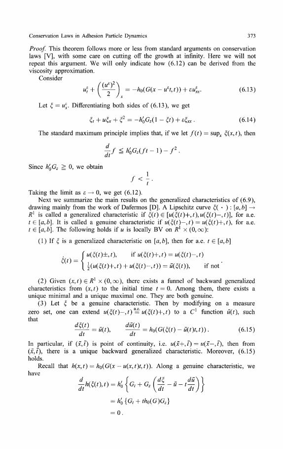
Conservation Laws in Adhesion Particle Dynamics 373
Proof. This theorem follows more or less from standard arguments on conservationlaws [V], with some care on cutting off the growth at infinity. Here we will notrepeat this argument. We will only indicate how (6.12) can be derived from theviscosity approximation.
Consider
( ^ ) -u%t)) + εuε
xx. (6.13)
Let ξ = ux. Differentiating both sides of (6.13), we get
ξt + uξx + ξ2 = -h'0Gz(l - ξt) + εξxx . (6.14)
The standard maximum principle implies that, if we let f{t) = supx ξ(x9t% then
dt
Since h'0G2 ^ 0, we obtain
ξ-fSh'0G2(ft-\)-f2.
/ < 7Taking the limit as ε -> 0, we get (6.12).
Next we summarize the main results on the generalized characteristics of (6.9),drawing mainly from the work of Dafermos [D]. A Lipschitz curve ξ{ ) : [a,b] —•Rι is called a generalized characteristic if ξ(t) e [u(ξ(t)-\-,t),u(ξ(t)—,t)], for a.e.t e [a9b]. It is called a genuine characteristic if u(ξ(t)—,t) = u(ξ(t)+9t)9 for a.e.t e [a,b]. The following holds if u is locally BV on Rι x (0,oo):
(1) If ξ is a generalized characteristic on [a9b]9 then for a.e. t G [a,b]
( u(ξ(t)±,t), if u(ξ(t)+,t) = u(ξ(t)-, t)
\ j(u(ξ(t)+, t) + u(ξ(t)-, 0 ) = ΰ(ξ(t)), if not'
(2) Given (x,t) £ Rι x (0, oo), there exists a funnel of backward generalizedcharacteristics from (x9t) to the initial time t = 0. Among them, there exists aunique minimal and a unique maximal one. They are both genuine.
(3) Let ξ be a genuine characteristic. Then by modifying on a measurezero set, one can extend u(ξ(t)—9t) = u(ξ(t)+9t) to a C1 function ΰ{t), suchthat
In particular, if (x9t) is point of continuity, i.e. u(x+9T) = u(x—9t)9 then from(x9t)9 there is a unique backward generalized characteristic. Moreover, (6.15)holds.
Recall that h(x9t) — ho(G(x - u(x9t)t9t)). Along a genuine characteristic, wehave
= h'0{Gt + th0(G)Gz}
= 0.

374 W. E, Yu.G. Rykov, Ya.G. Sinai
Part II. Behavior with Random Initial Data
7. Behavior of Solutions with Random Initial Data for Systems (1.1) and (1.2)
This part is devoted to the study of the qualitative behavior of solutions constructedabove when the initial data are random. We prove that the systems (1.1), (1.2), and(1.3) share the following common feature: For continuous but nowhere differentiablerandom initial data, almost surely, the solution u(x,t) becomes discontinuous for anyt > 0, the set of discontinuities (shocks) is dense (on the appropriate intervals), andalmost all masses are absorbed by the shocks. In particular for any t > 0, p( , t)becomes a discrete measure even though it may have a smooth distribution at t = 0.Such behavior was, to some extent, anticipated by Zeldovich [Z], as part of hisproposal for the formation of large scale structures in the universe. Technically, weextend some of the arguments in [S].
Let Q be the probability distribution of initial velocities, w(x;0) = uo(x). Weassume
(Ql) Q is defined on the Borel σ-algebra of the space of continuous functionson Rι, and for a.e. u$ (with respect to Q),
lim - ^ — = 0 .|jc|-»oo |X
(Q2) For a.e. w0, the following holds: for any η0 e Rι,
Jη
η°(u(η;0)-u(η0;0))dηlim sup— 7 = oo ,
λ->0+ hz
J^+\u(η;0)-u(η0;0))dηlim mf — Γ^ = —oo .
h^0+ hz
Concerning po> the initial distribution of masses, we will assume either
(1) po e Cι(Rι), 0 < const ^ po ^ const < oo, \p'\ ^ const < ooor
(2) poeCι(Rι), po(x) > 0 for xG(a9b)9 and po(x) = 0, for xe(a,b),\p'o(x)\ S const < oo. For (1.2) we will only consider the case (2).
Theorem 4. For a.e. u0, the weak solutions of(lΛ) and (1.2) constructed by GVPhave the following properties: For any t > 0,
(a) The measure Pt is a pure point measure, i.e. Pt(x) — J2i mi^(x ~ χiX(mi > 0).
(b) The closure of the set {xz} is either Rι in the case of (I), or a closedinterval 1(t) in the case of (2).
Proof We will only prove this theorem for (1.1). The modifications required for(1.2) are obvious.

Conservation Laws in Adhesion Particle Dynamics 375
We will show that for a.e. wo, the partition ξt given by GVP has the followingproperties:
i) There exists a countable set of elements of ξt which are intervals of positivelength.
ii) The union of these intervals is a set of full measureiii) Between any two of these intervals there are infinitely many similar intervals.
Clearly (i)-(iii) implies the theorem.Fix yo + a,b and take w( ;0) satisfying (Ql). Assume that yo is the left end
point of an element of ξt, i.e. for any h\, h2 > 0,
+ tu(η;O))po(η)dη
( 7 Λ )
We will show that the Q-probability of such u{ 0) is zero. Indeed we can rewrite(7.1) as
JvLh, in ~ yo)po(η)dη Γ° . (u(η\ 0) - u(y0; O))po(η)dη
Since po(yo) > 0, we have
Iy"-h](u{η; 0) - u(yQ;O))po(η)dη po(Jo)/^0-/,,(«(»/;0) ~ <W, 0))dη
y o \ £hι ~ Po(yo))dη
o \ (u(η; 0) ~ u(y0; O))(po(η) - Po(yo))dη
hι ~ po(yo))dη
° .(u(η;O)-u(yo;O))dηs h l ( 1 + (7.3)
Similar estimates hold for the integrals on (y0, yo + ti2 )• Therefore, we can write(7.1) as
Γ°+h2(u(η;0)-u(y0;0))dη^ ( l + ( l ) ) + O(h2). (7.4)
From (Q2), this can only hold on a ^-measure 0 set of u( 0).Next we consider the measurable space of (u( 0), yo) equipped with the prod-
uct measure of Q and the Lebesgue measure on Rι. The Fubini theorem implies thatfor Q — a.e. u( 0) the set of yo satisfying (7.4) has Lebesgue measure zero. Thisproves (ii). Since two different intervals in ξt cannot have a common end point,

376 W. E, Yu.G. Rykov, Ya.G. Sinai
there have to be infinitely many such intervals in between. Finally, since φt is acontinuous nondecreasing function, and φt is constant on each of these intervals,the range of φt from these intervals has to be dense on its full range.
8. Behavior of Solutions with Random Initial Data for (1.3)
In this section we prove an analogous result of Theorem 4 for the nonconservativemodel (1.3). We use mainly the method of characteristics, an approach potentiallymore general than the one used in Sect. 7. For the initial data we will assume thatPo £ C1 Π L 1 ^ 1 ) , and u( O) = wo( ) is random with distribution Q, satisfying(Ql), whereas (Q2) is replaced by a more stringent condition:
(Q2') There exists a function ω(h), such that for almost a.e. UQ,
ω(h)
^ ^ - l , (8.1)|Λ|—o ω(h)
holds for all y e Rι, and the convergence is uniform on compact sets. Moreover,ω satisfies
(1) lim ω(h) = 0, lim ^ ^ = +oo .|A|-0 |A|->0 h
(2) There exists a constant ε > 0, such that for any h > 0, one can find h\ > 0,such that ω(h\) < \ω(h) and h\ > εh.
(2) essentially says that ω has algebraic behavior near 0. Obviously, the Wienerprocess satisfies (Q2') with ω(h) = (2λlog | ) 1 / 2 .
Theorem 5. For α.e. wo, ίΛe wfl& solution of (13) constructed in Sect. 6 /zαs thefollowing properties: for any t > 0, /e/ {x/} be the set of shock locations at timet. Then
(a) The measure p( , 0 is a pure point measure: p(x,t) = Σz m^(x — xz),/w, ^ 0.
Proof Take w(x;0) such that (Ql) and (Q2;) are satisfied and fix any t* > 0. Wefirst show that the set of shock locations is dense in Rι. Assume to the contrarythat there exists an interval A on which u( , t*) is continuous. Then for any x G Athere is a unique backward characteristic ξ : [0,Γ] —> i?1 connecting x to a point jμat ί = 0. Furthermore, along ξ we have
— ξ(t) = ύ(t\ —h(ξ(t\t) = 0, —5(0 = -A({(0,0 (8.2)
Thus ξ is given by
t2
ζ(t) = y + ίwoίjO — o(.y)7r> ί(* ) — χ - (8-3)2
The mapping from y to x is obviously continuous. It is also one-to-one since thecharacteristics do not intersect between 0 and t*. Therefore, the inverse mapping
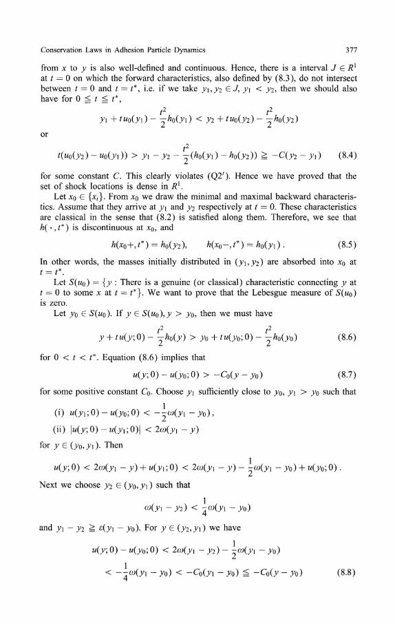
Conservation Laws in Adhesion Particle Dynamics 377
from x to y is also well-defined and continuous. Hence, there is a interval J £ Rι
at t = 0 on which the forward characteristics, also defined by (8.3), do not intersectbetween t — 0 and t = t*9 i.e. if we take y\,y2 G J, y\ < y2, then we should alsohave for 0 ^ t ^ /*,
t2 t2
y\ +tuo(y\)- -^ho(yχ) < y2 + tu0(y2)- -ho(y2)
or
t2
t(uo(y2) ~ u0(y0) > y\ - y2 - -(ho(yι)- ho(y2)) ^ -C(y2 - yx) (8.4)
for some constant C. This clearly violates (Q2'). Hence we have proved that theset of shock locations is dense in Rι.
Let xo G {x/}. From xo we draw the minimal and maximal backward characteris-tics. Assume that they arrive at y\ and y2 respectively at t = 0. These characteristicsare classical in the sense that (8.2) is satisfied along them. Therefore, we see thath( ,ί*) is discontinuous at xo, and
h(xo+,t*) - ho(y2\ h(xo-,t*) = h(yλ). (8.5)
In other words, the masses initially distributed in (y\,y2) are absorbed into xo att = t*.
Let S(uo) = {y : There is a genuine (or classical) characteristic connecting y att = 0 to some x at t = t*}. We want to prove that the Lebesgue measure of S(uo)is zero.
Let yo e S(uo). If y G S(uo),y > yo, then we must have
t2 t2
h() + ( 0)t t
y + tu(y; 0) - -ho(y) > y0 + ί«(^0; 0) - -Aoϋ>o) (8.6)
for 0 < t < t*. Equation (8.6) implies that
u(y;0) - u(yo O) > ~Co(y - yo) (8.7)
for some positive constant Q . Choose y\ sufficiently close to yo, y\ > yo such that
(i) u(yι\0) - u(yo\O) < ~-ω(yι - yo),
(ii) | U ( ^ ; 0 ) - M ( ^ I ; 0 ) | < 2ω(yx - y)
for y e (yo, y\). Then
u(y;0) < 2ω(yx -y) + u(yx;0) < 2ω(y{ - y) - -ω(yx - y0) + u(yo;O) .
Next we choose y2 G (,yo? J i ) such that
ω(^i - 72) < ^ωQ/i - 70)
and 7i - 32 ^ ε(ji — o) F° r ^ G (72,^1) we have
; 0) - w(j0; 0) < 2ω{y\ - y2) - -ω(yx - y0)
- ^ Φ i ~ .yo) < -C0(y\ - yo) ^ -C0(y - y0) (8.8)

378 W. E, Yu.G. Rykov, Ya.G. Sinai
if y\ is sufficiently close to yo. Comparing (8.8) with (8.7) we see that (y2,y\)eS(u0). Therefore, we have
\S(uo)n[yθ9yι]\ < χ_&
\[yo,y\\\
Here we used \A\ to denote the Lebesgue measure of the set A. Hence yo is not apoint of density of S(UQ). Since this is true for all y0 G S(UQ), we have |S(wo)| = 0.
Acknowledgements. We thank U. Frisch for numerous stimulating discussions related to the prob-lem discussed in this paper. The work by E was supported by the Sloan Foundation. The work ofYu. Rykov was supported, in part, by the Foundation of Fundamental Research of Russia underthe grant N 93-01-16090. The work of Ya. Sinai was partially supported by the National ScienceFoundation under grant DMS-9404437.
Appendix: Contact Points on the Convex Hull
In this appendix we summarize some properties of the contact points on the convexhull of 0i o φ~ι, extending the discussions in Sect. 2. We will assume that Po hasa density po(x),uo is continuous.
Definition Al. A point z is called special if
c(z,z) = min c(z,z+) = max c(z~,z) = c(z,z) .
Lemma Al. The set of special points is closed.
Proof. Let zn be a sequence of special points, zn —> z. We claim that z is a specialpoint. Assume to the contrary, then for some z~ < z < z+,
c(z~9z) > c(z,z+).
But c(z~,z) = limn-^oo c(z~,zn), c{z,z+) = \m\n^ooc{zmz+). Therefore, for suffi-ciently large n,
c(z~,zn) > c(zn,z+) ,
which contradicts our assumption that zn is a special point.
Definition A2. A special point z is called single if c(z,z+) > c(z~,z) for anyz~ < z < z+. A special point z is called multiple if there exists either z + > z forwhich c{z+,z) — c(z9z)9 or z~ < z for which c(z~,z) = c(z,z).
For every z consider a segment [ZJ~,ZQ~], where z ~ = min{y ^ z : c(y,z) —C(Z,Z)},ZQ = max{jμ ^ z : c(z,y) = c(z,z)}. If a point z is multiple then [ZQ~,ZQ~]has positive length.
Lemma A2. Take y e (z,z£) where c(z,y) > c(z,z). Then y is not a special point.
Proof. We have
c(z,z+) = p\c(z,y) +
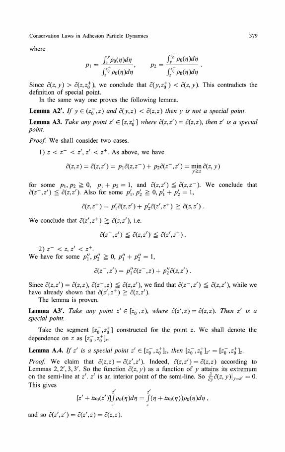
Conservation Laws in Adhesion Particle Dynamics 379
where
Jz
ypo(η)dη f/poWdηPi = -*+ , Pi = ~^
Jz°Po(η)dη Jz° Po(η)dη
Since c(z,y) > c{z,z^\ we conclude that C()?,ZQ) < c(z,y). This contradicts thedefinition of special point.
In the same way one proves the following lemma.
Lemma A2'. If y G (z^,z) and c(y,z) < c(z,z) then y is not a special point.
Lemma A3. Take any point z' G [Z,ZQ] where c{z,zf) = c{z,z\ then z1 is a specialpoint.
Proof. We shall consider two cases.
1) z < z~~ < z'9zr < z+. As above, we have
c(z,z) = c(z,z') = pιd(z,z~) + pic(z~9z') = min c(z,y)
for some pupi ^ 0, p\ + pi = 1, and c(z,zf) ^ c(z,z~). We conclude thatc(z~9z') ^ c(z,z'). Also for some pί,/?^ ^ 0, p[ -{- pf
2 = I,
c(z,z+) = p[c(z,z') + p'2c{z\z+) ^ c(z,zf) .
We conclude that c(z\z+) ^ c(z9zf), i.e.
2) z- < z, z7 < z+ .We have for some p'{9 p'{ ^ 0, p'[ + p'{ = I,
Since c(z,z') = c(z9z)9 c(z~9z) ^ c{z9z')9 we find that c(z",z7) ^ c{z9z')9 while wehave already shown that φ ^ z " ^ ^ φ j Z 7 ) .
The lemma is proven.
Lemma A37. Take any point zf e [ZQ,Z\ where c(z\z) = c(z9z). Then z1 is aspecial point.
Take the segment [z^~,zj] constructed for the point z. We shall denote the
dependence on z as [Z^",ZQ"]Z.
Lemma A.4. If V is a special point z' G [ZQ~,ZJ"]Z, then [z^~,z^]z/ = [z^~,zj"]z.
Proof We claim that c(z,z) = c(zf,zf). Indeed, c(z,zf) = c(z9z) according toLemmas 2,2/,3,3/. So the function c(z9y) as a function of y attains its extremum
j-c(z9y)\y=
ainson the semi-line at z1. z' is an interior point of the semi-line. So j-c(z9y)\y=zf = 0.This gives
\z' + tuQ(zf)-\jP(){η)dη = J(η + tuo(η))po(η)dη ,z z
and so c(z\z') — c(z'9z) = c(z,z).

380 W. E, Yu.G. Rykov, Ya.G. Sinai
S u p p o s e zι < z . W e h a v e , f o r s o m e p\,p2 ^ 0, p λ + p 2 = 1,
c(z,z) = C(ZQ,Z) = PIC(ZQ9Z') + p2c(z',z) = '
If we have z~ < z^ such that c(z~,z') = c(zf,z'), then for some p[9p2 ^ 0, p\ +
Pf2=h
c(z~,z) = p[c(z-,z') + p'2c{zf,z) = p[c(z',z) + /^Φ**) = Φ>*)
That contradicts our assumption that ZQ~ is the smallest with such a property. The
analogous calculations can be done with zjj".
The case z < z' can be analyzed in a similar way.
References
[BG] Brenier, Y., Grenier, E.: On the model of pressureless gases with sticky particles. Preprint,1995
[CPY] Carnevale, G.F., Pomeau, Y., Young, W.R.: Statistics of ballistic agglomeration. Phys.Rev. Lett., 64, no. 24, 2913 (1990)
[D] Dafermos, C: Generalized characteristics and the structure of solutions of hyperbolicconservation laws. Indiana Univ. Math. J. 26, 1097-1119 (1977)
[GMS] Gurbatov, S.N., Malakhov, A.N., Saichev, A.I.: Nonlinear Random Waves and Turbulencein Nondispersive Media: Waves, Rays and Particles. Manchester: Manchester UniversityPress, 1991
[KPS] Kofman, L., Pogosyan, D., Shandarin, S.: Structure of the universe in the two-dimensionalmodel of adhesion. Mon. Nat. R. Astr. Soc. 242, 200-208 (1990)
[L] Lax, P.D.: Hyperbolic systems of conservation laws: II. Comm. Pure. Appl. Math. 10,537-556 (1957)
[O] Oleinik, O.A.: Discontinuous solutions of nonlinear differential equations. Uspekhi Mat.Nauk. 12, 3-73 (1957)
[P] Peebles, P.J.E.: The Large Scale Structures of the Universe. Princeton, NJ: PrincetonUniversity Press, 1980
[SZ] Shandarin, S.F., Zeldovich, Ya.B.: The large-scale structures of the universe: Turbu-lence, intermittency, structures in a self-gravitating medium. Rev. Mod. Phys. 61, 185—220 (1989)
[SAF] She, Z.S., Aurell, E., Frisch, U.: The inviscid Burgers equation with initial data ofBrownian type. Commun. Math. Phys. 148, 623-641 (1992)
[S] Sinai, Ya.G.: Statistics of shocks in solutions of inviscid Burgers equation. Commun.Math. Phys. 148, 601-622 (1992)
[VDFN] Vergassola, M., Dubrulle, B., Frisch, U., Noullez, A.: Burgers' equation, devil's staircasesand the mass distribution function for large-scale structures. Astron & Astrophys 289,325-356 (1994)
[V] Volpert, A.I.: The space BV and quasilinear equations. Math. USSR-Sbornik. 2, 225-267(1967)
[Z] Zeldovich, Ya.B.: Gravitational instability: An approximate theory for large density per-turbations. Astron & Astrophys. 5, 84-89 (1970)
Communicated by J.L. Lebowitz