Generalized S Transform - ece.uvic.cafrodo/publications/gst.pdf · 2 Abstract The generalized S...

Generalized S Transform

Michael D. Adams, Member, IEEE, Faouzi Kossentini, Senior Member, IEEE, and

Rabab Ward, Fellow, IEEE

Dept. of Elec. and Comp. Engineering, University of British Columbia,

Vancouver, BC, Canada V6T 1Z4

Abstract

The generalized S transform (GST), a family of reversible integer-to-integer transforms inspired by the S transform, is

proposed. This family of transforms is then studied in detail, by considering topics such as GST parameter calculation, the

effects of using different rounding operators in the GST, and the relationship between the GST and the lifting scheme. Some

examples of specific transforms in the GST family are also given. In particular, a new transform in this family is introduced,

and its practical utility demonstrated.

EDICS Category: 3-COMP (Signal Representation and Compression)

Please address all correspondence concerning this manuscript to:

Michael D. Adams

Department of Electrical and Computer Engineering

University of British Columbia

2356 Main Mall

Vancouver, BC, Canada V6T 1Z4

Phone: 604-822-2872, Fax: 604-822-5949

Email: [email protected]

1

Generalized S Transform�

Michael D. Adams, Member, IEEE, Faouzi Kossentini, Senior Member, IEEE, and

Rabab Ward, Fellow, IEEE

�This work was supported by the Natural Sciences and Engineering Research Council of Canada.

November 28, 2001 DRAFT

2

Abstract

The generalized S transform (GST), a family of reversible integer-to-integer transforms inspired by the S transform, is

proposed. This family of transforms is then studied in detail, by considering topics such as GST parameter calculation, the

effects of using different rounding operators in the GST, and the relationship between the GST and the lifting scheme. Some

examples of specific transforms in the GST family are also given. In particular, a new transform in this family is introduced,

and its practical utility demonstrated.

I. INTRODUCTION

Reversible integer-to-integer transforms have become a popular tool for use in signal coding applications requir-

ing lossless signal reproduction [1–5]. One of the best known transforms of this type is the S transform [3,4,6]. In

this manuscript, we propose the generalized S transform (GST), a family of reversible integer-to-integer transforms

based on the key ideas behind the S transform. We then study the GST in some detail. This leads to a number of

interesting insights about transforms belonging to the GST family (including the S transform amongst others) and

reversible integer-to-integer transforms in general.

The remainder of this manuscript is structured as follows. We begin, in Section II, with a brief discussion of

the notation and terminology used herein. The S transform is then introduced in Section III, and the GST family

of transforms is defined in Section IV. Sections V and VI proceed to examine GST parameter calculation and

the effects of using different rounding operators in the GST. Some examples of well known transforms belonging

to the GST family are given in Section VII, and in Section VIII, we present a new GST-based transform, and

demonstrate its utility for image coding applications. Finally, we conclude in Section IX with a summary of our

results and some closing remarks.

II. NOTATION AND TERMINOLOGY

Before proceeding further, a short digression concerning the notation and terminology used in this manuscript

is appropriate. The symbols � and � denote the sets of integer and real numbers, respectively. Matrix and vector

quantities are indicated using bold type. The symbol �� is used to denote the �� identity matrix. In cases

where the size of the identity matrix is clear from the context, the subscript � may be omitted. A matrix is

said to be unimodular if �� . The �� th minor of the �� matrix , denoted !#"%$�&�'(�) �*�� , is the

�+�-,.�(�/�0�+�1,2�(� matrix formed by removing the � th row and � th column from . The notation 34'5��67� denotes

the probability of event 6 , and the notation 89��6:� denotes the expected value of the quantity 6 .

Suppose that ; denotes a rounding operator. In this manuscript, such operators are defined only in terms of a

single scalar operand. As a notational convenience, however, we use an expression of the form ;<��=>� , where = is


3

a vector/matrix quantity, to denote a vector/matrix for which each element has had the operator ; applied to it. A

rounding operator ; is said to be integer invariant if it satisfies

; ��6:�4� 6 for all 6 � � (1)

(i.e., ; leaves integers unchanged). As customary, in this manuscript, we consider only integer-invariant rounding

operators. For obvious reasons, rounding operators that are not integer invariant are of little practical value. At

times, we focus our attention on six specific rounding operators (i.e., the floor, biased floor, ceiling, biased ceiling,

truncation, and biased truncation functions) which are defined below.

For � � � , the notation� �� denotes the largest integer not more than � (i.e., the floor function), and the notation� �� denotes the smallest integer not less than � (i.e., the ceiling function). In passing, we also note that the floor

and ceiling functions satisfy the relationship

� �� , � ,�� for all � � �� (2)

The biased floor, biased ceiling, truncation, and biased truncation functions are defined, respectively, as

�� & &�'�� "��<� � �<,�� (3)

�*' ��$ � �<�!"# "$ � �� for �&%('� �� for �&)('�� and (4)

� �*' ��$ � �<�!"# "$ �� & &�'�� for �&%('�� "�� for �&)('� (5)

The mapping associated with the� �*' ��$ � function is essentially equivalent to traditional rounding (to the nearest

integer). The fractional part of a real number � is denoted *�' + � � and defined as

*�' + � �-,�.� , � ��/Thus, we have that '&0(* ' + � �1) � for all � � � . We define the ! & � function as

! & � ��6>�32��4,� 6 ,52 � 676829� where 6 � � �32 � � . (6)

This function simply computes the remainder obtained when 6 is divided by 2 , with division being defined in such

a way that the remainder is always nonnegative. From (6) and (2), we trivially have the identities

� 676829� �;:�<�=/>@?BAC:�D EGFE for 2IH�J' (7)� 676829� � :BKL=/>@?BAM<�:�D EGFE for 2IH�J'N (8)


4

III. S TRANSFORM

One of the simplest and most ubiquitous reversible integer-to-integer mappings is the S transform [2–4], a

nonlinear approximation to a particular normalization of the Walsh-Hadamard transform. The S transform is also

well known as the basic building block for a reversible integer-to-integer version of the Haar wavelet transform [2–

4]. The forward S transform maps the integer vector � :�� :�� to the integer vector � E � E � � � , and is defined most

frequently (e.g., equation (1) in [3] and equation (3.3) in [4]) as� E��E� � � �� A :�� KL:�� F� :��@<�:�� The corresponding inverse transform is given (e.g., equation (2) in [3]) by� :��: � � �� <�E �� where �4,�.2�� 2 � � �(� � (9)

While the S transform can be viewed as exploiting the redundancy between the sum and difference of two

integers, namely that both quantities have the same parity (i.e., evenness/oddness), this overlooks a much more

fundamental idea upon which the S transform is based. That is, as noted by Calderbank et al. [2], the S transform

relies, at least in part, on lifting-based techniques.

IV. GENERALIZED S TRANSFORM

By examining the S transform in the context of the lifting scheme, we are inspired to propose a natural extension

to this transform, which we call the generalized S transform (GST). For convenience in what follows, let us define

two integer vectors = and � as

= ,�� : � : �� :�� ,�� E � E �!�� E"� � � � � The forward GST is a mapping from = to � of the form��$# = � ;0�*�&% , �(�"# =>� � (10)

where % is real matrix of the form % ,�(')* �,+ � +.- �� + �� /� � �� ...

......

. . ....�/�0� ��

1324 �# is a unimodular integer matrix defined as

# ,�5')*�6 �87 � 6 �87 � 6 �87 - �� 6 �87 � � �6 �97 � 6 �97 � 6 �97 - �� 6 �97 � � �6 - 7 � 6 - 7 � 6 - 7 - �� 6 - 7 � � �......

.... . .

...6 � � �97 � 6 � � �97 � 6 �� 97 - �� 6 � � �97 � � �1324 �


5

and ; is a rounding operator. By examining (10), one can easily see that this transform maps integers to integers.

In the absence of the rounding operator ; , the GST simply degenerates into a linear transform with transfer matrix

, where ,��% # . Thus, the GST can be viewed as a reversible integer-to-integer mapping that approximates

the linear transform characterized by the matrix . The inverse GST is given by

= �$# < � �&� , ; � �&% , �(� � �� (11)

Note that # < � is an integer matrix, since, by assumption, # is a unimodular integer matrix. To show that (11) is,

in fact, the inverse of (10), one need only observe that due to the form of % , for any two � �� vectors � and � :

� � � � ;0�*�&% , �(� � � (12)

implies

� �� , ;0��&% ,0�(�� L (13)

By substituting � � # = and �� into (12) and (13), we obtain (10) and (11), respectively.

The GST can be realized using the networks shown in Figs. 1(a) and 1(b). These networks share some similar-

ities with the reversible integer-to-integer ladder networks described in [2, 5] (which, in turn, are related to ideas

in [7, 8]). This said, however, some differences also exist, as explained below.

The first difference can be attributed to the fact that we are dealing with � -input � -output networks, where �is potentially larger than two. In such cases, adjacent ladder steps that modify the same channel can be combined,

reducing the number of rounding operations and resulting quantization error. For example, suppose that we have

a � -input � -output network comprised of �+� , �(� ladder steps, all of which modify the ' th channel. Although

we could naively perform rounding separately for each ladder step, as shown in Fig. 2(a), the rounding error can

be significantly reduced by grouping the ladder steps together and performing rounding only once, as shown in

Fig. 2(b).

The second difference relates to the presence of the unimodular integer matrix # (or # < � ). In the case of the

lifting scheme, filtering is performed exclusively by a ladder network, while with the GST framework, filtering is

accomplished by the cascade of a ladder network and a linear network with a unimodular integer transfer matrix

(i.e., # or # < � ). This difference, however, is arguably less important, since a unimodular integer matrix can always

be decomposed into a product of elementary unimodular integer matrices and such a factorization is essentially a

lifting factorization. (The proof that a unimodular integer matrix can be decomposed into a product of elementary

unimodular integer matrices is constructive by the standard algorithm for computing the Smith normal form of an

integer matrix (e.g., as described in [9]).)


6

From a mathematical viewpoint, the specific strategy used to realize the transforms # and # < � is not particularly

critical. Since both transforms are linear, each has many equivalent realizations. These two transforms could be

implemented using ladder networks, as suggested above, but this is not necessary.

In passing, we would like to note that Hao and Shi [10] have done some related work with � -point block

transforms. Their work is concerned primarily with the lifting factorization problem for general block transforms,

whereas we study in detail a very specific class of these transforms (i.e., those belonging to the GST family). Thus,

the results presented herein and those presented in [10] are complementary. Other works, such as [1, 7], have also

considered reversible � -input � -output ladder networks in various contexts (where � % �). These other works,

however, do not specifically consider the GST family of transforms. Thus, our results are distinct from those in the

preceding works.

V. CALCULATION OF GST PARAMETERS

Suppose that we are given a linear transform characterized by the transform matrix , and we wish to find a

reversible integer-to-integer approximation to this transform based on the GST framework. In order for this to be

possible, we must be able to decompose as

� % # (14)

where the matrices % and # are of the forms specified in (10). Therefore, we wish to know which matrices have

such a factorization. The answer to this question is given by the theorem below.

Theorem 1 (Existence of GST Factorization) The real matrix , defined as

�,� '* � �87 � � �87 � �� 87 � � �� 97 � � �97 � �� 97 � � �......

. . ....� �� 97 � � � � �97 � �� 97 � � �

14 �has a GST factorization (i.e., a factorization of the form of (14)) if and only if all of the following conditions hold:

1. The last �-,2� rows of must contain only integer entries. That is,

�� D � � � for � � � � � � 5��-,2� �� J' � � � ��-,2� 2. is unimodular.

3. The integers �(�� ! " $�&�'(�) � ' �*� �� < �� are relatively prime.

Proof: First, we prove the sufficiency of the above conditions. We begin by considering the slightly more

general decomposition

� %�� # (15)


7

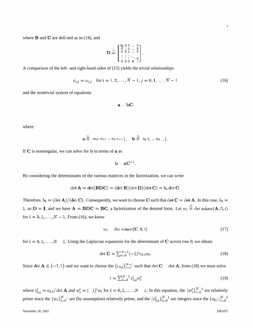
where % and # are defined as in (14), and

� ,� '* + � � � �� /� � �� ......

.... . . ��/� � � �

14 A comparison of the left- and right-hand sides of (15) yields the trivial relationships

� � D � � � � D � for � � � � � � 5��1,2� , � � ' � � � ��1,2� (16)

and the nontrivial system of equations

� � � #where

� ,� � � �87 � � �87 � �� 87 � � � � � � ,� � + � + � �� + �� If # is nonsingular, we can solve for

�in terms of � as

� � � # < � By considering the determinants of the various matrices in the factorization, we can write

�� (�&%�� # �4� �+�� % � �+�� +�� # � �� :�� # Therefore, � � � �+�� 36 �+�� # � . Consequently, we want to choose # such that �� # � �� . In this case, � � �� , so � � � , and we have � %�� # � % # , a factorization of the desired form. Let � � ,� �� !#"%$�&�'(�) � ' �*� �for � � ' � � � (��1,2� . From (16), we know

� � � �� ! "%$�&�'(� ##� ' �*� � (17)

for � � ' � � � (��1,2� . Using the Laplacian expansion for the determinant of # across row 0, we obtain

�� # �� < �� ,<�(� � � � D � � � (18)

Since �� , � � � � and we want to choose the � � � D � � � < �� such that �� # � �� , from (18) we must solve

� � � � < �� D � � �� (19)

where � � � D � � � � D � 6 �� and � �� ,<�(� � � � for � � ' � � � 5��1,.� . In this equation, the �� < �� are relatively

prime since the �� < �� are (by assumption) relatively prime, and the � �� D � � � < �� are integers since the � � � D � � � < �� November 28, 2001 DRAFT

8

are integers and �� ,<� � � � . We can show that (19) always has a solution. This result follows immediately

from the well known result in number theory that states: The greatest common divisor (GCD) of a set of integers

is a linear combination (with integer coefficients) of those integers, and moreover, it is the smallest positive linear

combination of those integers [11]. In our case, the integers �� < �� are relatively prime, so their GCD is � ,and therefore, 1 must be a linear combination of the integers �� < �� . Furthermore, the coefficients of the linear

combination can be found using the Euclidean algorithm [11]. Therefore, we can use (19) to generate a valid

choice for # , and knowing # , we can solve for�

, and hence find % . Thus, we have a constructive proof that the

desired factorization of exists. This shows the sufficiency of the above conditions on the matrix .

The necessity of the above conditions on the matrix is easily shown. Due to the form of % , the last � , �rows of the matrices and # must be the same. Thus, the last � , � rows of must contain only integer entries,

since # is an integer matrix. If is not unimodular, obviously it cannot be decomposed into a product of two

unimodular matrices (namely, % and # ). This follows from the fact that �� % �� # , �� % � � ,<� � � � ,and �� # � � , � � � � . The relative primeness of �(�� !#"%$�&�'(�) � ' �*� �� < �� follows from the “GCD is a linear

combination” theorem stated above. If this set of integers is not relatively prime, their GCD is greater than one,

and no solution to (19) can exist. Thus, the stated conditions on the matrix are necessary for a GST factorization

to exist.

From the proof of the above theorem, we know that the factorization is not necessarily unique, since more than

one choice may exist for the � � � D � � � < �� above. In instances where the solution is not unique, we can exploit this

degree of freedom in order to minimize the computational complexity of the resulting transform realization.

For most practically useful transforms in the GST family, it is often the case that �(! " $�&�'(�) � ' �*� �� < �� are all

unimodular (i.e., �� ! " $�&�' �) � ' �*� �� for all � � �B' � � � 5��, � � ). This condition holds for all of the

examples considered later in Section VII. In such instances, the most useful GST factorizations are often obtained

by choosing the unknowns � � � D � � � < �� so that all but one are zero, with the remaining unknown being chosen as

either ,<� or � in order to satisfy (19). In this way, we can readily obtain � distinct GST factorizations of which

typically yield low complexity transform realizations.

In all likelihood, the most practically useful transforms in the GST family are those for which the output 2 �is chosen to be a rounded weighted average of the inputs � 6 � � � < �� (with the weights summing to one) and the

remaining outputs � 2 � � � < �� are chosen to be any linearly independent set of differences formed from the inputs

� 6 � � � < �� . Such transforms are particularly useful when the inputs � 6 � � � < �� tend to be highly correlated.

Obviously, there are many ways in which the above set of differences can be chosen. Here, we note that two spe-

cific choices facilitate a particularly computationally efficient and highly regular structure for the implementation


9

of # (and # < � ). Suppose the difference outputs are selected in one of two ways:

type 1: 2 � � 6 � , 6 �type 2: 2 � � 6 � , 6 � < �

for �#�� , � . Since these differences completely define the last � , � rows of , we can calculate

�� ! "%$�&�'��) � ' � ' � . Furthermore, one can easily verify that in both cases �� ! "%$�&�'(�) � ' � ' � � � . Thus, we may

choose # for type-1 and type-2 systems, respectively, as

')* � �� < � � � �� < � � � �� ......

.... . . �< � ��

1324 and ')* � � � �� < � � � �� < �/� �� ...

......

. . . � �� < �/�

1324 Furthermore, we can show that the corresponding solutions for % are, respectively, given by

type 1: � � � � � D �type 2: � � � � � < �� D �

for � � � � � � (��1,2� .In the above cases, the transform matrices for # and # < � can be realized using the ladder networks shown

in Fig. 3. The forward and inverse networks for a type-1 system are shown in Figs. 3(a) and (b), respectively.

Similarly, the forward and inverse networks for a type-2 system are shown in Figs. 3(c) and (d). For each of the

two system types, the forward and inverse networks have the same computational complexity (in terms of the

number of arithmetic operations required).

Other choices of differences also facilitate computationally efficient implementations. Choices that yield a #matrix with all ones on the diagonal are often good in this regard.

VI. CHOICE OF ROUNDING OPERATOR

So far, we have made only one very mild assumption about the rounding operator ; (i.e., property (1) holds).

At this point, we now consider the consequences of a further restriction. Suppose that the rounding operator ;also satisfies

; ��6&�� 4� 6 � ; �� for all 6 � � , and all � � � (20)

(i.e., ; is integer-shift invariant). The operator ; could be chosen, for example, as the floor, biased floor, ceiling,

or biased ceiling operator (as defined in Section II). Note that the truncation and biased truncation operators are

not integer-shift invariant. To demonstrate this for either operator, one can simply evaluate the expressions on the


10

left- and right-hand sides of equation (20) for � � , �� and 6 � � . Clearly, the two expressions are not equal (i.e.,

' H� � or �&H�J' ).

If ; is integer-shift invariant, we trivially have the two identities shown in Fig. 4. Therefore, in the case that

; is integer-shift invariant, we can redraw each of the networks shown in Figs. 1(a) and 1(b) with the rounding

unit moved from the input side to the output side of the adder. Mathematically, we can rewrite (10) and (11),

respectively, as ��$# = � ;0�*�&% , �(�"# =>� (21a)

� ;0�8# = � �&% , �(�"# =>�� ;0�9% # =>� � and

= �$# < � � � , ; � �&% , �(� � �� (21b)

� , # < � � ;0��&% , �(� � � , � �� , # < � ;0�*�&% , �(� � , � �� , # < � ;0�*�&% , � �(� � �� , # < � ; � , % < � ��

Or alternately, in the latter case, we can write

= �$# < � ; � �&% < � � �where

; � �� ,� , ; � , � �@At this point, we note that ; and ; � must be distinct (i.e., different) operators. This follows from the fact that

a rounding operator cannot both be integer-shift invariant and satisfy ; �� , ; � , � � for all � � � . (See

Appendix I for a simple proof.) By using (2), we have, for the case of the floor and ceiling operations

; � ��67�4�

!"# "$ � 6 � for ; ��67� � � 6 �� 6 � for ; ��67�4� � 6 � The above results are particularly interesting. Recall that the GST approximates a linear transform characterized

by the matrix ,��% # . Examining the definition of the forward GST given by (10), we can see that, due to the

rounding operator ; , the underlying transform is a function of both % and # individually, and not just their

product . In other words, different factorizations of (into % and # ) do not necessarily yield equivalent


11

transforms. When ; is integer-shift invariant, however, (10) simplifies to (21a), in which case the underlying

transform depends only on the product . Thus, for a fixed choice of integer-shift invariant operator ; , all GST-

based approximations to a given linear transform (characterized by ) are exactly equivalent. This helps to explain

why so many equivalent realizations of the (original) S transform are possible, as this transform utilizes the floor

operator which is integer-shift invariant.

Computational Complexity

As one might suspect, the choice of rounding operator can affect computational complexity. In what follows, we

examine the effects of this choice for six different rounding operators (i.e., the floor, biased floor, ceiling, biased

ceiling, truncation, and biased truncation operators).

Consider the network of Fig. 2(b), the fundamental building block of the GST and also a much larger class of

reversible integer-to-integer N-input N-output mappings. This network simply computes the quantity

� � �� ; � � � < �� @ (22)

Without loss of generality1 , we assume that the gains � � � � � < �� can be expressed exactly as dyadic rational numbers

(i.e., numbers of the form :�� , where 6 � � ,� � � , and

� % � ). Provided that�

is chosen large enough, we can

always define�� ,� �� for � � � � � � 5�� ,2� where the � �� < �� . Often, in practice, we need to compute

the expression given by (22) using integer arithmetic. In such cases, we typically calculate

� � �� ; �� < ��

Thus, we must compute an expression of the form

; � :� � � (23)

where 6 � � .

Let us now consider the calculation of an expression of the form of (23) for each of the six rounding operators� Any given real number can be approximated with arbitrary accuracy by an appropriately chosen dyadic rational number.


12

mentioned above. Assuming a two’s complement integer representation, we can show that

� :� � � �J+��' ��6 � � � � �� & &�' :� � �.+��*'5��6&� � � � � �� :� � � �J+��' ��6&�� "�� :� � �J+��*' ��6-�� *' ��$ � � :� � �4�

!"# "$ +��*' ��6>� � � for 6 %('+��*' ��6-�� for 6 )(' and

� �*' ��$ � � :� � � �!"# "$ +��*' ��6-� � � � � for 6 %('+��*' ��6-�� for 6 )('�

where � � � � , � , � � � � < � , �� < � , � , and +��' ��6 ��>� denotes the arithmetic right shift of 6 by �

bits. The above expressions can be derived by observing that +��*' ��6>��>� � � :�� and� 676829� � � ��6&� 2 ,.�(�3682 � .

(See Appendix II for proofs of these assertions.) From above, we can see that the floor operator incurs the least

computation (i.e., one shift). The biased floor, ceiling, and biased ceiling operators require slightly more compu-

tation (i.e., one addition and one shift in total). Finally, the truncation and biased truncation operators are the most

complex due to their behavioral dependence on the sign of the operand.

Rounding Error

When constructing reversible integer-to-integer versions of linear transforms, one must remember that the effects

of rounding error can be significant. The objective is to produce a (nonlinear) integer-to-integer mapping that

closely approximates some linear transform with desirable properties. In order to preserve the desirable properties

of the parent linear transform, it is usually beneficial to minimize the error introduced by rounding intermediate

results to integers.

In the case of the GST, only one network of the form shown in Fig. 2(b) is employed. Thus, rounding is only

performed once, and the impact is relatively small. If, however, multiple networks of this form are cascaded

together (as in the case of more general lifting-based frameworks), rounding error may be more of a concern.

Therefore, in some applications, it may be desirable to choose the rounding operator in order to minimize rounding

error.

Suppose that we must round real numbers of the form :� � where 6 � � ,� � � , and

� % � . Such numbers are

associated with a fixed-point representation having�

fraction bits (i.e.,�

bits to the right of the binary point). If we

assume that, for both negative and nonnegative quantities, all� �

representable fractional values are equiprobable,

one can show that the error interval, peak absolute error (PAE), and mean absolute error (MAE) for each of the

rounding operators under consideration are as listed in Table I. (See Appendix III for the derivation of the error


13

intervals and MAE expressions. The PAE expressions follow immediately from the error intervals.) By examining

the table, one can easily see that, for� % �

, the biased rounding operators have the smallest MAEs and PAEs.

Consequently, the use of the biased operators has the advantage of reduced rounding error. It is important to note,

however, that the preceding assertion does not hold if� � � . (Typically, we would have

� � � when the � � � � � < �� in (22) are all integer multiples of one half.) If

� � � , all of the rounding operators under consideration have the

same PAE (i.e., �� ) and the same MAE (i.e., �� ), and consequently, all of these operators are equally good in terms

of rounding error. In practice, the case of� � � is not so unlikely to occur. Consequently, it is important to note

the peculiar behavior in this case. In fact, some well known papers on reversible integer-to-integer transforms have

overlooked this fact (and used a bias of one half when it is not beneficial to do so).

VII. EXAMPLES

One member of the GST family is, of course, the S transform. We can factor the transform matrix as �� % #where

�� < �� % � � � �� and# � � � �� < � � � � � �< � � � � � ��

The S transform is obtained by using the parameters from the above factorization for in the GST network in

conjunction with the rounding operator ; ��67� � � 6 � . (The particular network used to realize the matrix # is

indicated by the factorization of # shown above.) Mathematically, this gives us� E �E � � � � :�� K � �� where �4� 6 �/, 6 � � and (24a)� :��:�� E� K�� where � �.2 � , � E�� (24b)

Comparing (9) to (24b), we observe that the computational complexity of the latter expression is lower (i.e., one

less addition is required). Due to our previous results, however, we know that both equations are mathematically

equivalent. Thus, we have found a lower complexity implementation of the inverse S transform.

Another example of a transform from the GST family is the reversible color transform (RCT), defined in the

JPEG-2000 Part-1 standard [12] (and differing only in minor details from a transform described in [13]). Again,

we can factor the transform matrix as �� % # where

� �� < �� < � � � � % � � �� # � � � � �� < �/�� < � � � � � � � �< �/� ��

� � �� < � � � ��


14

The RCT is obtained by using the parameters from the above factorization for in the GST network in conjunction

with the rounding operator ; ��67� � � 6 � . (Again, the particular network used to realize the matrix # is indicated

by the factorization of # shown above.) Mathematically, this gives us� E��E�E - � �� :�� K � �� A � � K � � F � �� where � � : - <�:�� :��G<�:�� and (25a)� :��: �: - � � � � KLE -�� KLE� � where � �.2 � , � �� 2 � � 2 � � � (25b)

The formula given for the forward RCT in [12] is� E �E �E - � � � � �� A :��3K � :�� KL: - F� : - <�:��:��@<�:�� (26)

By comparing (25a) and (26), we observe that the computational complexity of the former expression is lower

(i.e., four adds and one shift are required instead of, say, four adds and two shifts). Thus, we have found a lower

complexity implementation of the forward RCT. Although the computational complexity is reduced by only one

operation, this savings is very significant in relative terms (since only six operations were required before the

reduction).

Recall that for integer-shift invariant rounding operators, multiple realization strategies often exist for a partic-

ular GST-based reversible integer-to-integer transform. In order to demonstrate this, we now derive an alternative

implementation of the RCT. To do this, we factor the transform matrix associated with the RCT (i.e., the matrix from above) as � % # where % � � <�� # � � � � �� < �/�� < � � � � � � � �� < � ��

� � ��< � � �� < � � �

� � � �� The alternative RCT implementation is obtained by using the parameters from the above factorization for in

the GST network in conjunction with the rounding operator ; ��67�9� � 6 � . (Again, the particular network used to

realize the matrix # is indicated by the factorization of # shown above.) The corresponding RCT implementation

is given by � E��E�E - � �� : - K � �� A�<�� K � � F � �� where � � : - <�: �� :�� <�:�� and� :��:��: - � � � � �3KLE -� �� where � � �� <�E�� E��@< � �� A�<�� E� KLE - F� One can see that the computational complexity of this alternative implementation is higher than the one proposed

in (25). In fact, it is likely that, due to the simple nature of the RCT, the implementation given by (25) is probably

the most efficient.


15

VIII. PRACTICAL APPLICATION

When compressing a color image, a multicomponent transform is often applied to the color components in

order to improve coding efficiency. Such a transform is frequently defined so that one of its output components

approximates luminance. In this way, one can easily extract a grayscale version of a coded image if so desired.

For RGB color imagery, luminance is related to the color component values by

2 � 'N �� 'N�� 'N%�� (28)

where 2 is the luminance value, and � , � , and � are the red, green, and blue component values, respectively.

The forward RCT is defined in such a way that one of its output components approximates luminance. In effect,

the RCT computes the luminance as �� &� �� . Obviously, this is a rather crude approximation to the true

luminance as given by (28). Without a huge sacrifice in complexity, however, we can define a new RCT-like

transform that provides a much better approximation to true luminance. To this end, we propose a slightly altered

version of the RCT called the modified RCT (MRCT).

The forward and inverse equations for the MRCT are given, respectively, by� E��E�E - � �� : � K � �� A � � � K �� F� � �� where � � : � <�: �� : - <�:�� and (29a)� :��:��: - � � � � �� KLE - � where � � E�� < � �� A � E� K �� E - F �� 3KLE� � (29b)

The MRCT is associated with the transform matrix

�� < � � �� < � � � �

which can be factored as �� % # , where% � � �� # � � � � �< � � �� < �/� � �� < �/� ��

� � � �� < � � � The MRCT is obtained by using the above factorization for in the GST network in conjunction with the rounding

operator ; ��67� � � 6 � . (The particular network used to realize the matrix # is indicated by the factorization of# shown above.) The forward and inverse MRCT can each be implemented with six adds and four shifts (where

expressions of the form � �� '��&� �� can be computed as +��*'5�*� �� , �(�� 1� � � � � � � �� ). Recall that the

forward and inverse RCT, as given by (25), each require four adds and one shift. Thus, in terms of computational

complexity, the MRCT compares quite favorably with the RCT, when one considers the RCT’s extreme simplicity.

Having defined the MRCT, we first studied its coding performance. A set of 196 RGB color images, covering

a wide variety of content, was compressed losslessly using both the MRCT and RCT in the same coding system.


16

The difference in the overall bit rate obtained with the two transforms was less than 0.1%. Thus, the MRCT and

RCT are quite comparable in terms of coding efficiency.

In addition to coding efficiency, we also examined the luminance approximation quality. For each image, we

computed the true luminance component as given by (28) and the luminance components generated by the MRCT

and RCT. We then proceeded to calculate the approximation error for each transform. The results for several of the

test images are shown in Table II. Clearly, the MRCT approximates true luminance much more accurately than the

RCT (in terms of both MAE and PAE). Furthermore, this difference in approximation quality is usually visually

perceptible. That is, the MRCT yields a luminance component that appears visually identical to the true luminance

component, while the RCT generates a luminance component that is often visibly different from the ideal.

When designing the MRCT, we had to choose which set of differences to employ (for the two non-luminance

outputs of the forward transform). In passing, we would like to note that this choice can impact coding efficiency.

For natural imagery, experimental results suggest that the difference between the red and blue components is often

slightly more difficult to code than the other two differences (i.e., green-blue and green-red). For this reason, we

chose to use the green-blue and green-red differences to form the non-luminance outputs of the (forward) MRCT.

IX. CONCLUSIONS

The generalized S transform (GST), a family of reversible integer-to-integer transforms, was proposed. Then,

the GST was studied in some detail, leading to a number of interesting results. We proved that for a fixed choice of

integer-shift invariant rounding operator, all GST-based approximations to a given linear transform are equivalent.

Also, we studied several common rounding operators, examining their computational complexity and rounding

error properties. When considering both computational complexity and rounding error characteristics together,

the floor, biased floor, ceiling, and biased ceiling operators are arguably the most practically useful of those con-

sidered. The floor operator is desirable as it has the lowest computational complexity, while the biased floor and

biased ceiling operators are slightly more computationally complex but normally have the best rounding error

performance.

The S transform and RCT were shown to be specific instances of the GST. Lower complexity implementations

of the S transform and RCT were also suggested. A new transform belonging to the GST family, called the MRCT,

was introduced, and shown to be practically useful for image coding applications. Due to its utility, the GST family

of transforms will no doubt continue to prove useful in both present and future signal coding applications.


17

APPENDICES

I. ANTISYMMETRY AND INTEGER-SHIFT INVARIANCE

Proposition 1: A rounding operator ; that is integer-shift invariant cannot also possess the antisymmetry prop-

erty (i.e., ; �� , ; � , � � for all � � � ).

Proof: Consider the quantity ; � �� . Using trivial algebraic manipulation and the integer-shift invariance

property, we have

; � �� ;<� � , �� ;<� , �� (30)

From the antisymmetry property, we can write

; �8�� , ; � , �� (31)

Combining (30) and (31), we obtain

� � ; � , �� , ; � , �� ; � , �� Thus, we have that ; � , �� 6� � . Since, by definition, ; must always yield an integer result, the integer-shift

invariance and antisymmetry properties cannot be simultaneously satisfied by ; .

II. RELATIONSHIPS INVOLVING THE FLOOR OR CEILING FUNCTION

Proposition 2: Suppose that 6 is an integer represented in two’s complement form with a word size of � bits.

Let +��*' ��6>��>� denote the quantity resulting from the arithmetic right shift of 6 by � bits. We assert that

+��*' ��6>��>�4�� :�� where ' 0�� 0�� ,2� (32)

Proof: Let � � � � � � � �� < � denote the � bits of the word representing 6 , where � � and �� < � are the least-

and most-significant bits, respectively. In two’s complement form, the integer 6 is represented as

6 � , � � < � � � < � � �� < �� (33)

Through the properties of modular arithmetic, one can show that

! & � ��6>� �� < �� for '-0��50�� , � (34)


18

From the definition of the arithmetic shift right operation, we can write (for '&0�� 0�� ,2� )

+��' ��6 ��>�4� , � � < � � � < � � � � < �� < �� < � < � �

� � �� < � < �� K � � �

� , � � < � � � � < � , � � < � � � � < � < � �3�� < � < �� K � � �

� , � � < � � � < � < � � �� < � < �� K � � �

Using simple algebraic manipulation, (7), and (34), we can further rearrange the preceding equation as follows:

+��*' ��6>��>�4� , � � < � � � < � < � � �� < � < �� < � � � K � � � ,

� < �� < � � � K � ��

� �� , � � < � � � < � � �� < �� , �� ! & � ��6 � � � �

�;:�<�=/>@? A :�D � F�� :��

Thus, the identity given in (32) holds.

Proposition 3: For all 6 � � and all 2 � � except 2 � ' , the following identity holds:

� 676829� � � ��6 � 2 ,2�(�36829� (35)

Proof: One can easily confirm that the ! & � function satisfies the relationships

! & � ��6 �32��4� 6 for '-026 0 2 ,2� and 2IH�J' � and

! & � ��6&� 2 �32��4� ! & � ��6>�32��@From the two preceding properties, we can deduce

! & �>� ,/6 �32�� .2 ,2� , ! & � ��6 ,2� �32�� for 2IH�J'� (36)

Now we consider the expression on the right-hand side of equation (35). Using (7), we can write

� ��6 � 2 ,2�(��6829� � � ��6 ,2�(�36829� � � (37)

� �)6 � 2 ,2�/, ! & � ��6 ,2� �32��*� 682 Using (8) and (36), we can further manipulate (37) as follows:

� ��6 � 2 ,2�(�36829� � ��6&� ! & � � ,/6 �32��*��682#� � 6�682 � Thus, the identity given in (35) holds.


19

III. ROUNDING ERROR DERIVATIONS

Proposition 4: Consider the quantity :� � where 6 is a random integer and�

is a strictly positive integer constant.

If we suppose that *�' + � :� � may assume all� �

(distinct) possible values, then the error incurred by rounding the

quantity :�� using the the floor, biased floor, ceiling, biased ceiling, truncation, and biased truncation operators, is

bounded as follows:

, � � < �� 0 � :� � � , :� � 0(' � , � � � � < �� 0 �� & &�' � :� � � , :� � 0 �� '-0 � :� � � , :� � 0 � � < �� , �� 0 �� "�� :� � � , :� � 0 � � � � < �� (38)

, � � < �� 0 �*' ��$ � � :� � � , :� � 0 � � < �� and , �� 0 � �*' ��$ � � :� � � , :� � 0 �� If we further suppose that all

� �possible values of *�' + � :� � are equiprobable for � ) ' and are also equiprobable

for � % ' , then rounding :�� with the floor, biased floor, ceiling, biased ceiling, truncation, and biased truncation

operators incurs the respective mean absolute errors:

8 �� :�� , :�� < �� 8 �� & &�'(� :�� , :��

� � � �� 8 � �� :� � � , :� � �

� � � � � < �� 8 � �� "��)� :� � � , :� � �� (39)

8 �� *' ��$ � � :�� , :�� < �� and 8 �� *'@��$ � � :�� , :��

� � � �� Proof: From (6) and (2), we can show that the rounding error incurred by the floor, biased floor, ceiling, and

biased ceiling operators is, respectively, given by:

� :�� , :�� < =/>@?BAC:�D � � F�� (40)

� &�&�' � :� � � , :� � � � � � � <�=/> ?8A � � � � KL:�D � � F� � (41)

� :� � � , :� � � =/> ?8A�<�:�D � � F� � (42)

�� "�� :� � � , :� � �;=/>@?BA � � � � <�:�D � � F < � � � �� (43)

Using the definitions of the �*' ��$ � and� �*' ��$ � functions given by (4) and (5), respectively, and the identities (40)–

(43), we can easily deduce:

�*' ��$ � � :� � � , :� � �!"# "$ < =/>@?BAC:�D � � F� � for 6 %('=/> ?8A�<�:�D � � F� � for 6 )(' (44)

� �*' ��$ � � :� � � , :� � �!"# "$� � � � <�=/> ?8A � � � � KL:�D � � F� � for 6 % '=/> ?�A � � � � <�:�D � � F < � � � �� for 6 ) ' (45)


20

Since ! & � �� 6 � � � � and ! & � � � � < � �26 � �� can assume any integer value on � ' � � � , � � , we can easily deduce

all of the error bounds in (38) from (40)–(45). For example, consider the case of the floor operator. The rounding

error in this case is given by (40). Clearly, the minimum value of the rounding error is , � � < �� (occurring when

! & �>��6 � �� ,.� ). Similarly, the maximum value of the rounding error is ' (occurring when ! & � ��6 � � � � �' ). Thus, we have that ,

� � < �� 0 � :� � � , :� � 0J' . The remaining error bounds in (38) can be shown to hold in a

similar manner.

Now, let us consider the mean absolute error expressions for the various rounding operators. Since, by assump-

tion, all� �

possible values for *�' + � :� � are equiprobable, we know that ! & �>�� 6 � � � � and ! & � � � � < � � 6 � �� are both uniformly distributed over the integer values on � ' � � � , � � . Consequently, in the case of the floor, bi-

ased floor, ceiling, and biased ceiling operators, the mean absolute error can be found by computing the expected

value over the� �

possible absolute error values (associated with the� �

distinct fractional parts) using (40)–(45).

Straightforward analysis and algebraic manipulation yield the following:

8 � �� :� � � , :� � �� 8

�� < =/>@?BAC:�D � � F� � �

��

� � < ��

� < �� < �� (46)

8 �� & &�'(� :� � � , :� � �� 8

��

� � � � <�=/>@?BA � � � � KL:�D � � F� � ��

� � < ��

��

� � � � < �� (47)

8 �� :� � � , :� � �� 8

�� =/> ?8A�<�:�D � � F� � �

��

� � < ��

�� < �� (48)

8 � �� "��)� :� � � , :� � �� 8

�� =/> ?8A � � � � <�:�D � � F < � � � ��

��

� � < ��

��

� < � � � �� (49)

Let us now consider the mean absolute error for the �*' ��$ � function. From (46), (48), and the definition of the

�*' ��$ � function in (4), it follows that

8 � �� *' ��$ � � :� � � , :� � �� 3 ' � :� � )(' � 8 � �� :� � � , :� � �

� :� � ) ' � � 3 '(� :� � %(' � 8 � �� :� � � , :� � �� :� � % ' � (50)

Since, by assumption, all� �

possible values of *�' + � :� � are equiprobable for :� � )(' , we have from (48)

8 � �� :� � � , :� � �� :� � ) ' � � � � < �� (51)

Similarly, since all� �

possible values of *�' + � :� � are assumed to be equiprobable for :� � % ' , we have from (46)

that

8 � �� :� � � , :� � �� :� � %(' � � � � < �� (52)


21

By substituting (51) and (52) into (50) and then observing that 34'(� :�� )(' � � 3 '(� :�� %(' �4� � , we obtain

8 � �� *'@��$ � � :� � � , :� � �� 3 '(� :� � )(' � � � < �� 34'(� :� � %(' � � � < �� < ��

Therefore, the identity in (39) for the truncation operator holds.

Consider now the mean absolute error for the biased truncation operator. From (47), (49), and the definition of

the� �*' ��$ � function in (5), it follows that

8 � �� *'@��$ � � :� � � , :� � �� 3 ' � :� � )(' � 8 � �� "��)� :� � � , :� � �

� :� � ) ' � (53)

� 34'(� :� � %(' � 8 �� & &�'(� :� � � , :� � �� :� � %(' �

Since, by assumption, all� �

possible values of *�' + � :� � are equiprobable for :� � )(' , we have from (49) that

8 � �� "��)� :� � � , :� � �� :� � )(' � � �� (54)

Similarly, since all� �

possible values of * '@+ � :�� are equiprobable for :�� % ' , we have from (47) that

8 � �� & &�'(� :� � � , :� � �� :� � %(' � � �� (55)

By substituting (54) and (55) into (53) and observing that 3 ' � :� � )(' � � 3 ' � :� � %(' �4� � , we obtain

8 � �� *' ��$ � � :� � � , :� � �� 34'(� :� � )(' � � �� 3 ' � :� � %(' � � �� (56)

Therefore, the identity in (39) for the biased truncation operator holds. Thus, we have shown that all of the

identities in (39) hold.

ACKNOWLEDGMENT

The authors would like to thank Dr. Hongjian Shi and the anonymous reviewers for their useful comments and

suggestions.

REFERENCES

[1] M. D. Adams, “Reversible wavelet transforms and their application to embedded image compression,” M.A.Sc. thesis, Department

of Electrical and Computer Engineering, University of Victoria, Victoria, BC, Canada, Jan. 1998, Available from http://www.

ece.ubc.ca/˜mdadams.

[2] A. R. Calderbank, I. Daubechies, W. Sweldens, and B.-L. Yeo, “Wavelet transforms that map integers to integers,” Applied and

Computational Harmonic Analysis, vol. 5, no. 3, pp. 332–369, July 1998.

[3] A. Said and W. A. Pearlman, “An image multiresolution representation for lossless and lossy compression,” IEEE Trans. on Image

Processing, vol. 5, no. 9, pp. 1303–1310, Sept. 1996.


22

[4] A. Zandi, J. D. Allen, E. L. Schwartz, and M. Boliek, “CREW: Compression with reversible embedded wavelets,” in Proc. of IEEE

Data Compression Conference, Snowbird, UT, USA, Mar. 1995, pp. 212–221.

[5] H. Chao, P. Fisher, and Z. Hua, “An approach to integer wavelet transforms for lossless for image compression,” in Proc. of

International Symposium on Computational Mathematics, Guangzhou, China, Aug. 1997, pp. 19–38.

[6] P. Lux, “A novel set of closed orthogonal functions for picture coding,” Archiv fur Elektronik und Uebertragungstechnik, vol. 31, no.

7, pp. 267–274, July 1977.

[7] F. A. M. L. Bruekers and A. W. M. van den Enden, “New networks for perfect inversion and perfect reconstruction,” IEEE Journal

on Selected Areas in Communications, vol. 10, no. 1, pp. 130–137, Jan. 1992.

[8] W. Sweldens, “The lifting scheme: A custom-design construction of biorthogonal wavelets,” Applied and Computational Harmonic

Analysis, vol. 3, no. 2, pp. 186–200, 1996.

[9] R. S. Garfinkel and G. L. Nemhauser, Integer Programming, John Wiley and Sons, Toronto, 1972.

[10] P. Hao and Q. Shi, “Matrix factorizations for reversible integer mapping,” IEEE Trans. on Signal Processing, vol. 49, no. 10, pp.

2314–2324, Oct. 2001.

[11] J. E. Shockley, Introduction to Number Theory, Holt, Rinehart, and Winston, Toronto, 1967.

[12] ISO/IEC, ISO/IEC 15444-1, Information technology — JPEG 2000 image coding system — Part 1: Core coding system, 2001.

[13] M. J. Gormish, E. L. Schwartz, A. F. Keith, M. P. Boliek, and A. Zandi, “Lossless and nearly lossless compression of high-quality

images,” in Proc. of SPIE, San Jose, CA, USA, Mar. 1997, vol. 3025, pp. 62–70.


23

� K

�

� K� K

��

��

��

� �

��

��

�

��

��

�

�� E��E�E -�: -:��:�� .� ��.� ��.� �

...

�.� ��.� � + � � �+.-+ � E"�� .� �......

......

...:�� ......

(a)

� K

�

� K� K

�

�

��

��

��

� �

��

��

�

��

� � �

<� �� :��

: -:�� .�� .�� .�E��E�E -� �.� + � � �+.-+ � :�� .�� .�

E"� � � ......

......

......

......

(b)Fig. 1. Network realization of the generalized S transform. (a) Forward transform and (b) inverse transform.

� K � K

� � �

� K��

�

� �

�

� �

�

��

�

��

� � �

��

��

� �� -

+ � +.-

� �.�� .�� .�� .� + � � �

� � -

� �.�� .�...

......

......

......

......

...� ��

(a)

� K

�

� K� K

��

��

� �

��

��

�

��

� � �

��

�

� �.�� .�� .�� -

� �.� + � � �+.-+ � � �.�� .�

� �� ......

......

......

...

� �� - �...

(b)

Fig. 2. Network for a group of ladder steps having the same output channel with rounding performed for (a) each ladder stepseparately, and (b) all of the ladder steps together.

TABLE IERROR CHARACTERISTICS FOR VARIOUS ROUNDING OPERATORS (FOR � �� )

Operator Error Interval PAE MAEExact For Large

�Exact For Large

�Exact For Large

�floor � , � � < �� ' � � ,<� � ' � � � < ��

� � < �� bfloor � , � � � � < �� , �� ceiling � ' � � � < �� ' � �(� � � < �� < �� bceil � , �� < �� , �� N�� trunc � , � � < �� < �� ,<� � �(� � � < �� < �� btrunc � , �� N�� , ��


24

� K � K� K

��

�

�

��

�

��

��

�� - < <...

- � �...

�.� ��.� ��.� �... < � � �� .� �(a)

� K� K

� K��

� � �

��

��

� � �

� -� �� ...

�.� ��.� ��.� � - � �

...... �.� � � � � � � � �

(b)

� K� K

� K� K

��

��

��

��

��

��

�

��

��

� �.�� .�� .�� .�� .�

�� - �� - ...

� -� ��

......

< <

� � -...

<<

(c)

� K � K� K

� K��

��

��

��

��

�

��

��

� �.�� -

� �...

� �.�� .�� .�� .�...

� � � -......

- � � - � � � � ��

(d)

Fig. 3. Networks for realizing particular forms of the � and �� matrices. The networks for type-1 systems: (a) forwardand (b) inverse networks. The networks for type-2 systems: (c) forward and (d) inverse networks.

� K�

� K �< � < ��

��

�

��

�

: E : E�

<

� K�

� K ��

�

��

�

��

: E : E

Fig. 4. Transformations for integer-shift invariant rounding operator.

TABLE IIDEVIATION FROM THE TRUE LUMINANCE FOR THE MRCT AND RCT

MRCT RCTImage MAE PAE MAE PAEflowers 0.654 1.635 6.515 25.326food 0.734 1.777 8.860 34.821sailboat 0.566 1.438 1.888 20.580tile 0.776 1.369 9.591 14.560


Generalized S Transform - ece.uvic.cafrodo/publications/gst.pdf · 2 Abstract The generalized S...

Documents

Transcript of Generalized S Transform - ece.uvic.cafrodo/publications/gst.pdf · 2 Abstract The generalized S...