IRS/Actuary Actuary’s Perspective by Alan E. Kaliski, FCAS, MAAA.
Upload
derrick-doyleCategory
view
230download
0
Generalized Minimum Bias Models
By
Luyang Fu, Ph. D.
Cheng-sheng Peter Wu, FCAS, ASA, MAAA

Agenda
History and Overview of Minimum Bias Method
Generalized Minimum Bias Models
Conclusions
Mildenhall’s Discussion and Our Responses
Q&A
History on Minimum Bias
A technique with long history for actuaries: – Bailey and Simon (1960)– Bailey (1963)– Brown (1988)– Feldblum and Brosius (2002)– In the Exam 9.
Concepts:– Derive multivariate class plan parameters by minimizing a
specified “bias” function
– Use an “iterative” method in finding the parameters

History on Minimum Bias
Various bias functions proposed in the past for minimization
Examples of multiplicative bias functions proposed in the past:
ji jiji
jijiji
jijijiji
jijijiji
yxw
yxrwBiasSquaredChi
yxrwBiasSquared
yxrwBiasBalanced
, ,
2,,
2
,,,
,,,
)(
)(
)(
History on Minimum Bias
Then, how to determine the class plan parameters by minimizing the bias function?
One simple way is the commonly used “iterative” method for root finding:
– Start with a random guess for the values of xi and yj
– Calculate the next set of values for xi and yj using the root finding formula for the bias function
– Repeat the steps until the values converge
Easy to understand and can program in almost any tools
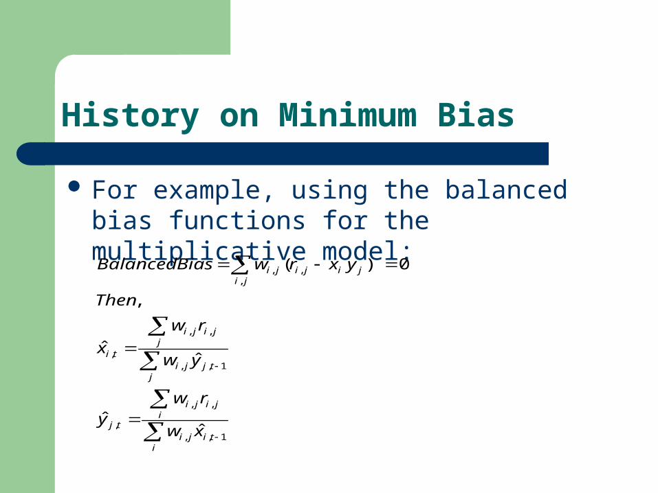
History on Minimum Bias
For example, using the balanced bias functions for the multiplicative model:
itiji
ijiji
tj
jtjji
jjiji
ti
jijijiji
xw
rwy
yw
rw
x
Then
yxrwBiasBalanced
1,,
,,
,
1,,
,,
,
,,,
ˆˆ
ˆˆ
,
0)(
History on Minimum Bias
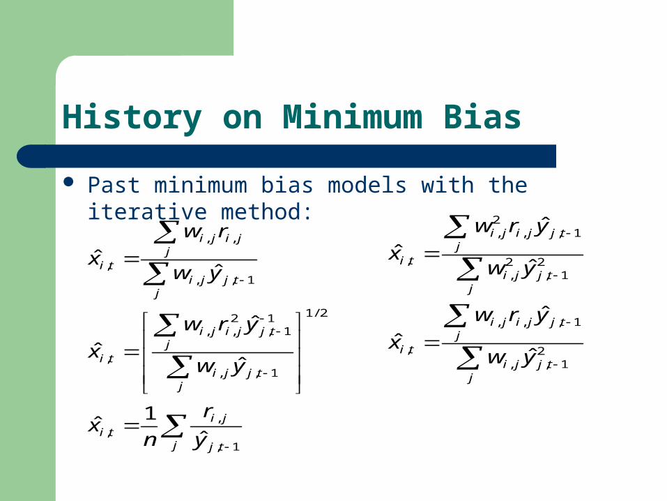
Past minimum bias models with the iterative method:
j tj
jiti
jtjji
jtjjiji
ti
jtjji
jjiji
ti
y
r
nx
yw
yrw
x
yw
rw
x
1,
,,
2/1
1,,
11,
2,,
,
1,,
,,
,
ˆ1
ˆ
ˆ
ˆ
ˆ
ˆˆ
jtjji
jtjjiji
ti
jtjji
jtjjiji
ti
yw
yrw
x
yw
yrw
x
21,,
1,,,
,
21,
2,
1,,2,
,
ˆ
ˆ
ˆ
ˆ
ˆ
ˆ

Issues with the Iterative Method
Two questions regarding the “iterative” method:– How do we know that it will converge?– How fast/efficient that it will converge?
Answers:– Numerical Analysis or Optimization textbooks– Mildenhall (1999)
Efficiency is a less important issue due to the modern computation power

Other Issues with Minimum Bias
What is the statistical meaning behind these models?
More models to try?Which models to choose?

Summary on Minimum Bias
A non-statistical approachBest answers when bias functions are
minimized Use of “iterative” method for root finding
in determining parametersEasy to understand and can program in
many tools
Minimum Bias and Statistical Models
Brown (1988) – Show that some minimum bias functions can be
derived by maximizing the likelihood functions of corresponding distributions
– Propose several more minimum bias models Mildenhall (1999)
– Prove that minimum bias models with linear bias functions are essentially the same as those from Generalized Linear Models (GLM)
– Propose two more minimum bias models
Minimum Bias and Statistical Models
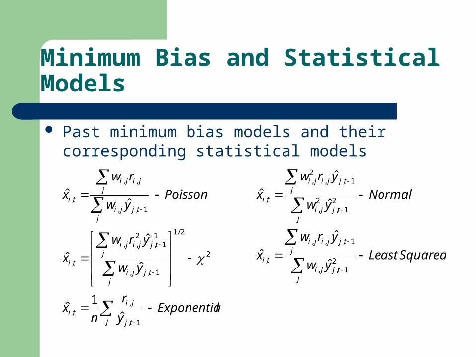
Past minimum bias models and their corresponding statistical models
lExponentiay
r
nx
yw
yrw
x
Poissonyw
rw
x
j tj
jiti
jtjji
jtjjiji
ti
jtjji
jjiji
ti
ˆ
1ˆ
ˆ
ˆ
ˆ
ˆ
ˆ
1,
,,
2
2/1
1,,
11,
2,,
,
1,,
,,
,
SquaredLeastyw
yrw
x
Normalyw
yrw
x
jtjji
jtjjiji
ti
jtjji
jtjjiji
ti
ˆ
ˆ
ˆ
ˆ
ˆ
ˆ
21,,
1,,,
,
21,
2,
1,,2,
,
Statistical Models - GLM
Advantages include:– Commercial softwares and built-in procedures available– Characteristics well determined, such as confidence level– Computation efficiency compared to the iterative procedure
Issues include:– Required more advanced knowledge for statistics for GLM
models– Lack of flexibility:
Rely on the commercial softwares or built-in procedures Assume the distribution of exponential families. Limited distribution selections in popular statistical software. Difficult to program yourself

Motivations for Generalized Minimum Bias Models
Can we unify all the past minimum bias models?
Can we completely represent the wide range of GLM and statistical models using Minimum Bias Models?
Can we expand the model selection options that go beyond all the currently used GLM and minimum bias models?
Can we improve the efficiency of the iterative method?
Generalized Minimum Bias Models
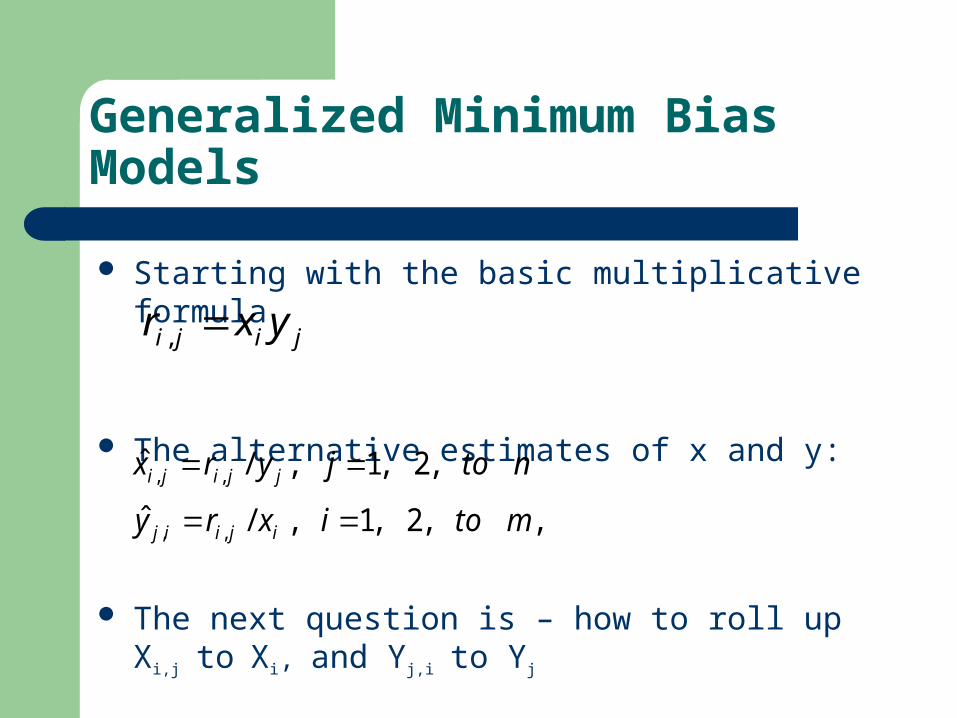
Starting with the basic multiplicative formula
The alternative estimates of x and y:
The next question is – how to roll up Xi,j to Xi, and Yj,i
to Yj
jiji yxr ,
,,2,1,/ˆ
,2,1,/ˆ
,,
,,
mtoixry
ntojyrx
ijiij
jjiji
Possible Weighting Functions
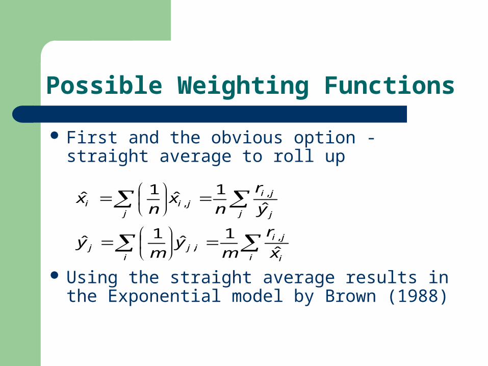
First and the obvious option - straight average to roll up
Using the straight average results in the Exponential model by Brown (1988)
i i
jiij
ij
j j
jiji
ji
x
r
my
my
y
r
nx
nx
ˆ1
ˆ1
ˆ
ˆ1
ˆ1
ˆ
,,
,,

Possible Weighting Functions
Another option is to use the relativity-adjusted exposure as weight function
This is Bailey (1963) model, or Poisson model by Brown (1988).
iiji
ijiji
i
ji
ii
iji
ijiij
ii
iji
ijij
jjji
jjiji
j
ji
jj
jji
jjiji
jj
jji
jjii
xw
rw
x
r
xw
xwy
xw
xwy
yw
rw
y
r
yw
ywx
yw
ywx
ˆˆˆ
ˆˆ
ˆ
ˆˆ
ˆˆˆ
ˆˆ
ˆ
ˆˆ
,
,,,
,
,,
,
,
,
,,,
,
,,
,
,

Possible Weighting Functions
Another option: using the square of relativity-adjusted exposure
This is the normal model by Brown (1988).
iiji
iijiji
iji
iiji
ijij
jjji
jjjiji
jij
jjji
jjii
xw
xrwy
xw
xwy
yw
yrw
xyw
ywx
22,
,2,
,22,
22,
22,
,2,
,22,
22,
ˆ
ˆˆ
ˆ
ˆˆ
ˆ
ˆ
ˆˆ
ˆˆ
Possible Weighting Functions
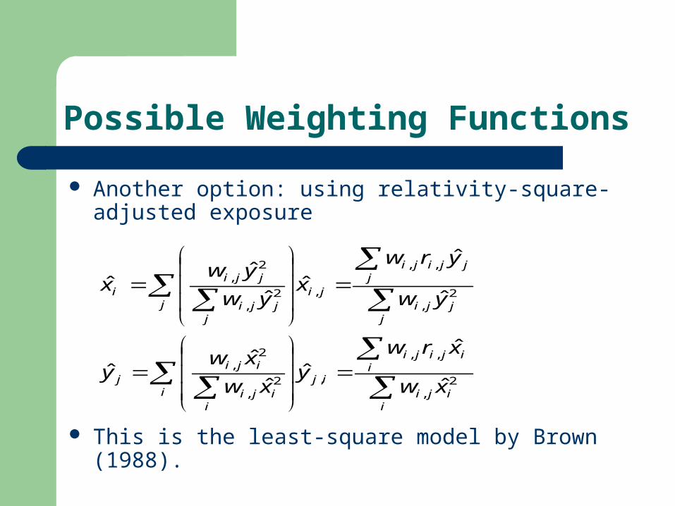
Another option: using relativity-square-adjusted exposure
This is the least-square model by Brown (1988).
iiji
iijiji
iji
iiji
ijij
jjji
jjjiji
jij
jjji
jjii
xw
xrwy
xw
xwy
yw
yrw
xyw
ywx
2,
,,
,2,
2,
2,
,,
,2,
2,
ˆ
ˆˆ
ˆ
ˆˆ
ˆ
ˆ
ˆˆ
ˆˆ

Generalized Minimum Bias Models
So, the key for generalization is to apply different “weighting functions” to roll up Xi,j to Xi and Yj,i to Yj
Propose a general weighting function of two factors, exposure and relativity:WpXq and WpYq
Almost all published to date minimum bias models are special cases of GMBM(p,q)
Also, there are more modeling options to choose since there is no limitation, in theory, on (p,q) values to try in fitting data – comprehensive and flexible

2-parameter GMBM
2-parameter GMBM with exposure and relativity adjusted weighting function are:
i
qi
pji
i
qiji
pji
iji
i
qi
pji
qi
pji
j
j
qj
pji
j
qjji
pji
jij
j
qj
pji
qj
pji
i
xw
xrwy
xw
xwy
yw
yrw
xyw
ywx
1,
1,,
,,
,
,
1,,
,,
,
ˆ
ˆˆ
ˆ
ˆˆ
ˆ
ˆ
ˆˆ
ˆˆ
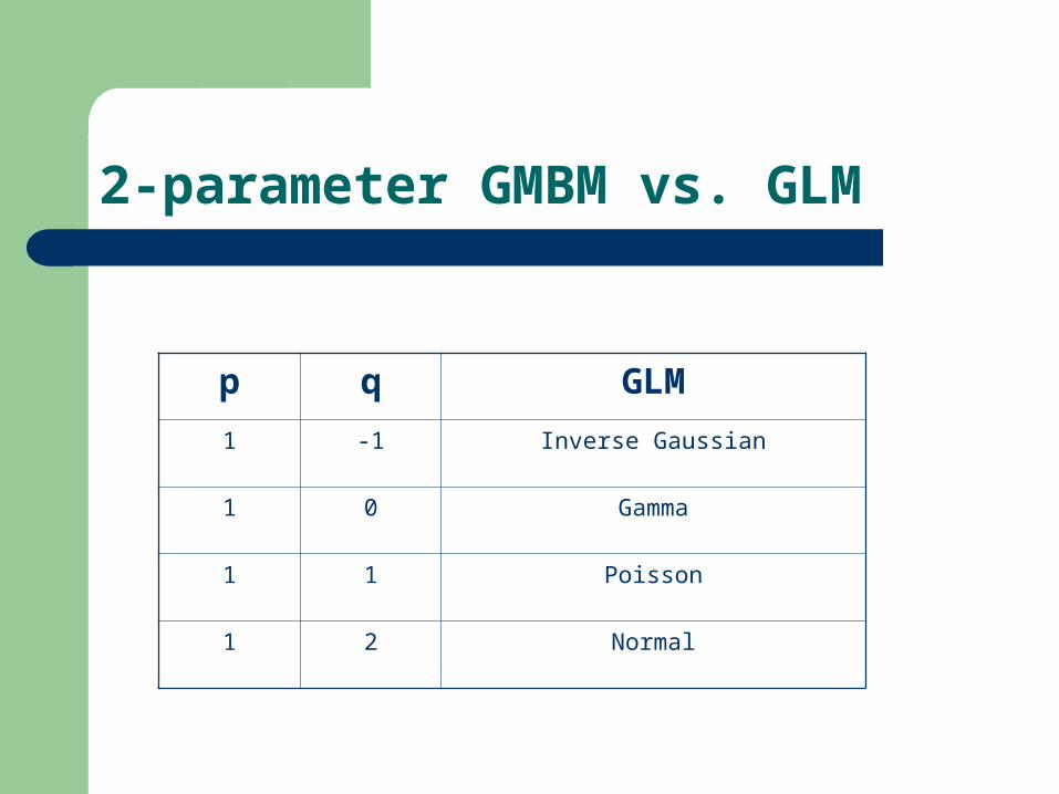
2-parameter GMBM vs. GLM
p q GLM
1 -1 Inverse Gaussian
1 0 Gamma
1 1 Poisson
1 2 Normal

2-parameter GMBM and GLM
GMBM with p=1 is the same as GLM model with the variance function of
Additional special models:– 0<q<1, the distribution is Tweedie, for pure premium models– 1<q<2, not exponential family– -1<q<0, the distribution is between gamma and inverse
Gaussian After years of technical development in GLM and
minimum bias, at the end of day, all of these models are connected through the game of “weighted average”.
qV 2)(

3-parameter GMBM
One model published to date not covered by the 2-parameter GMBM: Chi-squared model by Bailey and Simon (1960)
Further generalization using a similar concept of link function in GLM, f(x) and f(y)
Estimate f(x) and f(y) through the iterative method
Calculate x and y by inverting f(x) and f(y)
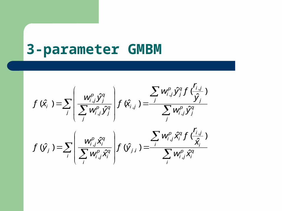
3-parameter GMBM
i
qi
pji
i i
jiqi
pji
iji
i
qi
pji
qi
pji
j
j
qj
pji
j j
jiqj
pji
jij
j
qj
pji
qj
pji
i
xw
x
rfxw
yfxw
xwyf
yw
y
rfyw
xfyw
ywxf
ˆ
)ˆ
(ˆ
)ˆ(ˆ
ˆ)ˆ(
ˆ
)ˆ
(ˆ
)ˆ(ˆ
ˆ)ˆ(
,
,,
,,
,
,
,,
,,
,
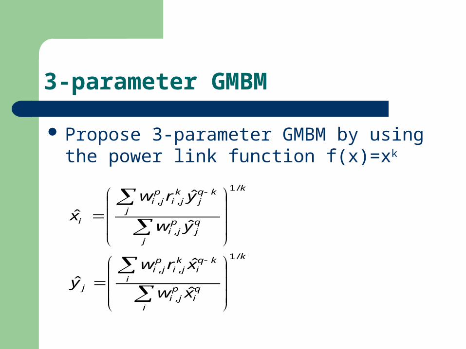
3-parameter GMBM
Propose 3-parameter GMBM by using the power link function f(x)=xk
k
i
qi
pji
i
kqi
kji
pji
j
k
j
qj
pji
j
kqj
kji
pji
i
xw
xrwy
yw
yrw
x
/1
,
,,
/1
,
,,
ˆ
ˆˆ
ˆ
ˆ
ˆ
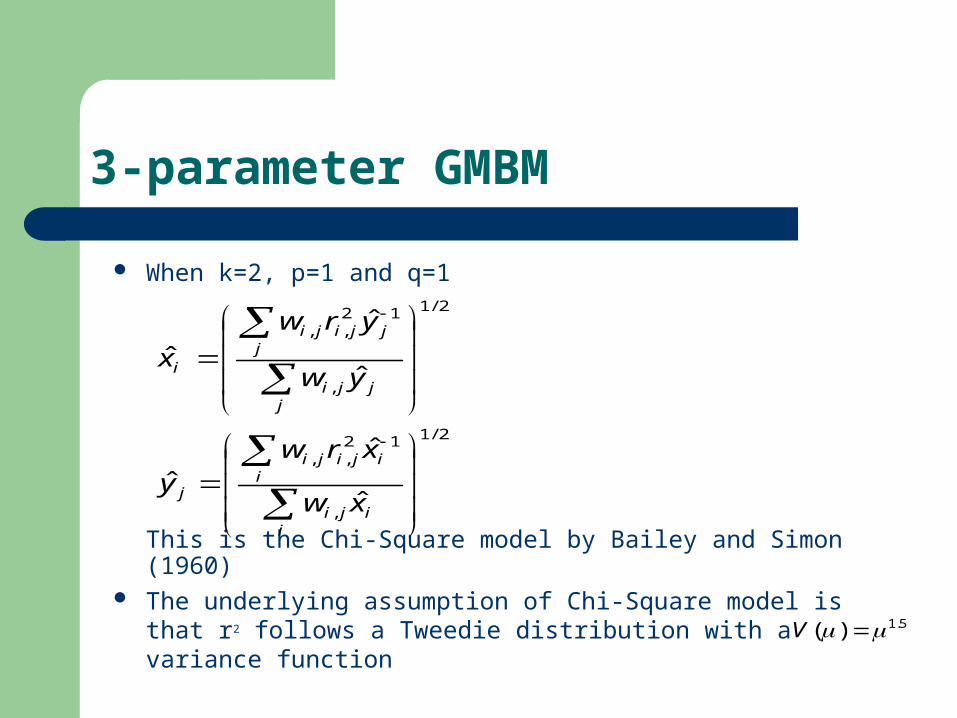
3-parameter GMBM
When k=2, p=1 and q=1
This is the Chi-Square model by Bailey and Simon (1960) The underlying assumption of Chi-Square model is that r2
follows a Tweedie distribution with a variance function
2/1
,
12,,
2/1
,
12,,
ˆ
ˆˆ
ˆ
ˆ
ˆ
iiji
iijiji
j
jjji
jjjiji
i
xw
xrwy
yw
yrw
x
5.1)( V
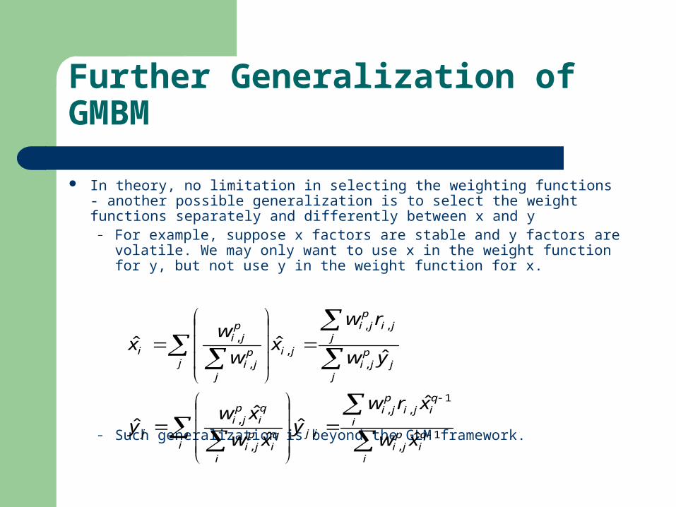
Further Generalization of GMBM
In theory, no limitation in selecting the weighting functions - another possible generalization is to select the weight functions separately and differently between x and y
– For example, suppose x factors are stable and y factors are volatile. We may only want to use x in the weight function for y, but not use y in the weight function for x.
– Such generalization is beyond the GLM framework.
i
qi
pji
i
qiji
pji
iji
i
qi
pji
qi
pji
j
jj
pji
jji
pji
jij
j
pji
pji
i
xw
xrwy
xw
xwy
yw
rw
xw
wx
1,
1,,
,,
,
,
,,
,,
,
ˆ
ˆˆ
ˆ
ˆˆ
ˆˆˆ

Numerical Methodology for the Iterative Method
Use the mean of the response variable as the base Starting points:
Use the latest relativities in the iterations
All the reported GMBMs converge within 8 steps
x
yi
j
,
,
0
0
1
1
itiji
ijiji
tj
jtjji
jjiji
ti
xw
rwy
yw
rw
x
,,
,,
,
1,,
,,
,
ˆˆ
ˆˆ
A Severity Case Study
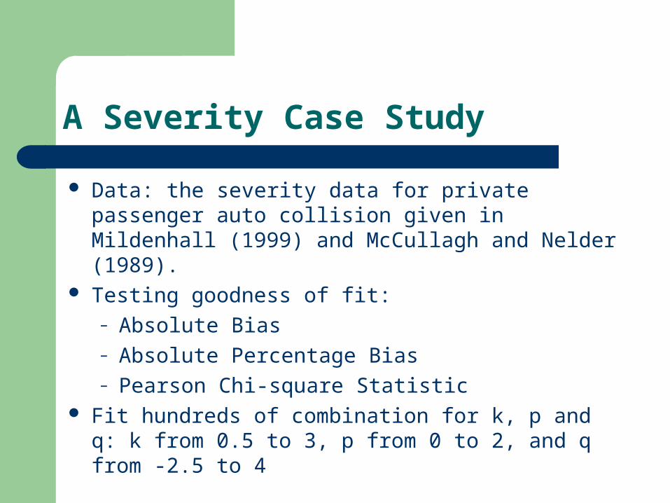
Data: the severity data for private passenger auto collision given in Mildenhall (1999) and McCullagh and Nelder (1989).
Testing goodness of fit:– Absolute Bias– Absolute Percentage Bias– Pearson Chi-square Statistic
Fit hundreds of combination for k, p and q: k from 0.5 to 3, p from 0 to 2, and q from -2.5 to 4
A Severity Case Study
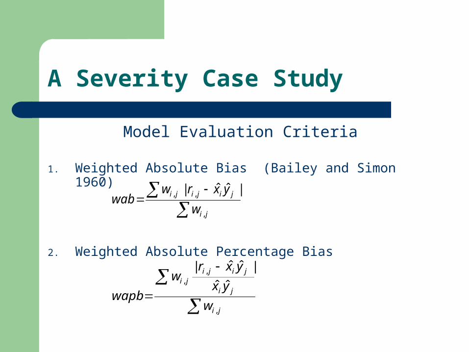
Model Evaluation Criteria
1. Weighted Absolute Bias (Bailey and Simon 1960)
2. Weighted Absolute Percentage Bias
ji
jijiji
w
yxrwwab
,
,, |ˆˆ|
ji
ji
jijiji
w
yx
yxrw
wapb,
,, ˆˆ
|ˆˆ|
A Severity Case Study
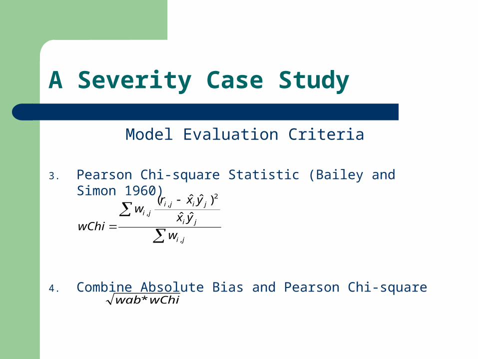
Model Evaluation Criteria
3. Pearson Chi-square Statistic (Bailey and Simon 1960)
4. Combine Absolute Bias and Pearson Chi-square
wChiwab*
ji
ji
jijiji
w
yx
yxrw
wChi,
2,
, ˆˆ
)ˆˆ(

A Severity Case Study
Best Fits
Criterion p q k
wab 2 0 3
wapb 2 0 3
Chi-square 1 1 2
combined 1 -0.5 2.5

Conclusions
• 2 and 3 Parameter GMBM can completely represent GLM models with power variance functions
• All published to date minimum bias models are special cases of GMBM
• GMBM provide additional model options for data fitting• Easy to understand and does not require advanced
statistical knowledge• Can program in many different tools• Calculation efficiency is not a issue because of
modern computer power.
Mildenhall’s Discussion
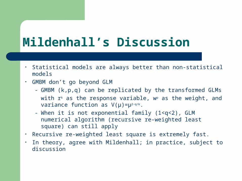
• Statistical models are always better than non-statistical models• GMBM don’t go beyond GLM
- GMBM (k,p,q) can be replicated by the transformed GLMs
with rk as the response variable, wp as the weight, and variance function as V(μ)=μ2-q/k.
- When it is not exponential family (1<q<2), GLM numerical algorithm (recursive re-weighted least square) can still apply
• Recursive re-weighted least square is extremely fast.• In theory, agree with Mildenhall; in practice, subject to
discussion

Our Responses to Mildenhall’s Discussion
Are statistical models always better in practice?• Require at least intermediate level of statistical
knowledge. • Statistical model results can only be provided by
statistical softwares. For example, GLM is very difficult to implement in Excel without additional software
• Popular statistical softwares provide limited distribution selections.
Our Responses to Mildenhall’s Discussion
Are statistical models always better in practice?• Few softwares provide solutions for distributions
with other power variance functions, such as Tweedie and non-exponential distributions
• It requires advanced statistical and programming knowledge to program the above distributions using the recursive re-weighted least square algorithm
• Costs involved acquiring softwares and knowledge
Our Responses to Mildenhall’s Discussion
Calculation Efficiency Recursive re-weighted least square algorithm
converges with fewer iterations. GMBM also converges fast with actuarial data. It
generally converges within 20 iterations by our experience.
The cost in additional convergence is small and the timing difference between GMBM and GLM is negligible with modern powerful computers.

Q & A