Generalized Linear Models in R – Geyer - Statistics ﬁnish the speciﬁcation of a...

Generalized Linear Models in R

Charles J. Geyer

December 8, 2003

This used to be a section of my master’s level theory notes. It is a bitoverly theoretical for this R course. Just think of it as an example of literateprogramming in R using the Sweave function. You don’t have to absorb all thetheory, although it is there for your perusal if you are interested.

1 Bernoulli Regression

We start with a slogan

• Categorical predictors are no problem for linear regression. Just use“dummy variables” and proceed normally.

but

• Categorical responses do present a problem. Linear regression assumesnormally distributed responses. Categorical variables can’t be normallydistributed.

So now we learn how to deal with at least one kind of categorical response, thesimplest, which is Bernoulli.

Suppose the responses are

Yi ∼ Bernoulli(pi) (1)

contrast this with the assumptions for linear regression

Yi ∼ Normal(µi, σ2) (2)

andµ = Xβ (3)

The analogy between (1) and (2) should be clear. Both assume the data areindependent, but not identically distributed. The responses Yi have distribu-tions in the same family, but not the same parameter values. So all we needto finish the specification of a regression-like model for Bernoulli is an equationthat takes the place of (3).

1

1.1 A Dumb Idea (Identity Link)

We could use (3) with the Bernoulli model, although we have to change thesymbol for the parameter from µ to p

p = Xβ.

This means, for example, in the “simple” linear regression model (with oneconstant and one non-constant predictor xi)

pi = α + βxi. (4)

Before we further explain this, we caution that this is universally recognized tobe a dumb idea, so don’t get too excited about it.

Now nothing is normal, so least squares, t and F tests, and so forth makeno sense. But maximum likelihood, the asymptotics of maximum likelihoodestimates, and likelihood ratio tests do make sense.

Hence we write down the log likelihood

l(α, β) =n∑

i=1

[yi log(pi) + (1− yi) log(1− pi)

]and its derivatives

∂l(α, β)∂α

=n∑

i=1

[yi

pi− 1− yi

1− pi

]∂l(α, β)

∂β=

n∑i=1

[yi

pi− 1− yi

1− pi

]xi

and set equal to zero to solve for the MLE’s. Fortunately, even for this dumbidea, R knows how to do the problem.

Example 1.1 (Bernoulli Regression, Identity Link).We use the data in the file ex12.8.1.dat in this directory, which is read by thefollowing

> X <- read.table("ex12.8.1.dat", header = TRUE)

> names(X)

[1] "y" "x" "z"

> attach(X)

and has three variables x, y, and z. For now we will just use the first two.The response y is Bernoulli. We will do a Bernoulli regression using the

model assumptions described above. The following code does the regressionand prints out a summary.

2

> out.quasi <- glm(y ~ x, family = quasi(variance = "mu(1-mu)"),

+ start = c(0.5, 0))

> summary(out.quasi, dispersion = 1)

Call:glm(formula = y ~ x, family = quasi(variance = "mu(1-mu)"), start = c(0.5,

0))

Deviance Residuals:Min 1Q Median 3Q Max

-1.552 -1.038 -0.678 1.119 1.827

Coefficients:Estimate Std. Error z value Pr(>|z|)

(Intercept) -0.354863 0.187324 -1.894 0.0582 .x 0.016016 0.003589 4.462 8.1e-06 ***---Signif. codes: 0 ‘***’ 0.001 ‘**’ 0.01 ‘*’ 0.05 ‘.’ 0.1 ‘ ’ 1

(Dispersion parameter for quasi family taken to be 1)

Null deviance: 137.19 on 99 degrees of freedomResidual deviance: 126.96 on 98 degrees of freedomAIC: NA

Number of Fisher Scoring iterations: 9

We have to apologize for the rather esoteric syntax, which results from ourchoice of introducing Bernoulli regression via this rather dumb example.

As usual, our main interest is in the table labeled Coefficients:, whichsays the estimated regression coefficients (the MLE’s) are α = −0.34750 andβ = 0.01585. This table also gives standard errors, test statistics (“z values”)and P -values for the two-tailed test of whether the true value of the coefficientis zero.

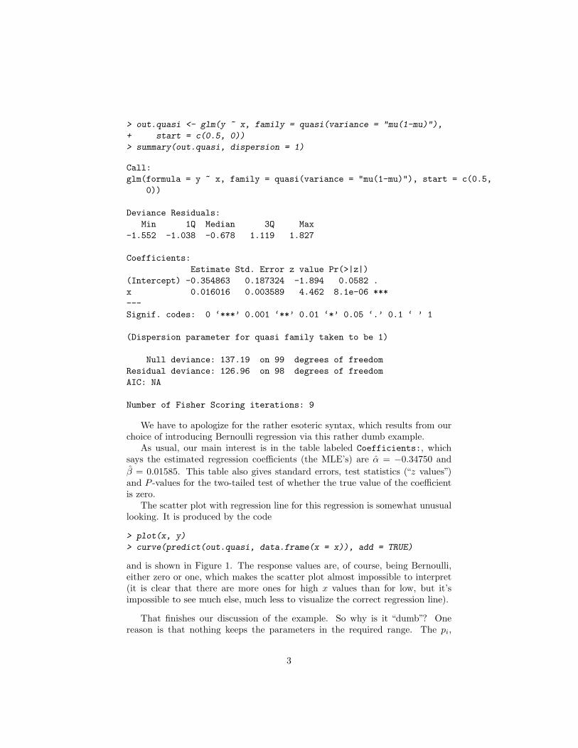
The scatter plot with regression line for this regression is somewhat unusuallooking. It is produced by the code

> plot(x, y)

> curve(predict(out.quasi, data.frame(x = x)), add = TRUE)

and is shown in Figure 1. The response values are, of course, being Bernoulli,either zero or one, which makes the scatter plot almost impossible to interpret(it is clear that there are more ones for high x values than for low, but it’simpossible to see much else, much less to visualize the correct regression line).

That finishes our discussion of the example. So why is it “dumb”? Onereason is that nothing keeps the parameters in the required range. The pi,

3

●

●

●

● ●

●●● ●●

●●

●

●

● ●●

● ● ●●

●●

● ●

● ●

●●

●

● ●

● ●●

●●

●●

●

●● ●

●●

●

●

●● ●

●

●

● ●

●

● ●

● ●

●●

●●●

●

● ●

●

●●

●●

● ●

●●

●

●●

● ●●● ●●

●

●

●●

● ●●

●

●

●

●

●

● ●

●

30 40 50 60 70 80

0.0

0.2

0.4

0.6

0.8

1.0

x

y

Figure 1: Scatter plot and regression line for Example 1.1 (Bernoulli regressionwith an identity link function).

4

being probabilities must be between zero and one. The right hand side of (4),being a linear function may take any values between −∞ and +∞. For thedata set used in the example, it just happened that the MLE’s wound up in(0, 1) without constraining them to do so. In general that won’t happen. Whatthen? R being semi-sensible will just crash (produce error messages rather thanestimates).

There are various ad-hoc ways one could think to patch up this problem.One could, for example, truncate the linear function at zero and one. But thatmakes a nondifferentiable log likelihood and ruins the asymptotic theory. Theonly simple solution is to realize that linearity is no longer simple and give uplinearity.

1.2 Logistic Regression (Logit Link)

What we need is an assumption about the pi that will always keep thembetween zero and one. A great deal of thought by many smart people came upwith the following general solution to the problem. Replace the assumption (3)for linear regression with the following two assumptions

η = Xβ (5)

andpi = h(ηi) (6)

where h is a smooth invertible function that maps R into (0, 1) so the pi arealways in the required range. We now stop for some important terminology.

• The vector η in (5) is called the linear predictor.

• The function h is called the inverse link function and its inverse g = h−1

is called the link function.

The most widely used (though not the only) link function for Bernoulli re-gression is the logit link defined by

g(p) = logit(p) = log(

p

1− p

)(7a)

h(η) = g−1(η) =eη

eη + 1=

11 + e−η

(7b)

Equation (7a) defines the so-called logit function, and, of course, equation (7b)defines the inverse logit function.

For generality, we will not at first use the explicit form of the link functionwriting the log likelihood

l(β) =n∑

i=1

[yi log(pi) + (1− yi) log(1− pi)

]

5

where we are implicitly using (5) and (6) as part of the definition. Then

∂l(β)∂βj

=n∑

i=1

[yi

pi− 1− yi

1− pi

]∂pi

∂ηi

∂ηi

∂βj

where the two partial derivatives on the right arise from the chain rule and areexplicitly

∂pi

∂ηi= h′(ηi)

∂ηi

∂βj= xij

where xij denotes the i, j element of the design matrix X (the value of the j-thpredictor for the i-th individual). Putting everything together

∂l(β)∂βj

=n∑

i=1

[yi

pi− 1− yi

1− pi

]h′(ηi)xij

These equations also do not have a closed form solution, but are easily solvednumerically by R

Example 1.2 (Bernoulli Regression, Logit Link).We use the same data in Example 1.1. The R commands for logistic regressionare

> out.logit <- glm(y ~ x, family = binomial)

> summary(out.logit)

Call:glm(formula = y ~ x, family = binomial)


-1.5237 -1.0192 -0.7082 1.1341 1.7665


(Intercept) -3.56633 1.15954 -3.076 0.00210 **x 0.06607 0.02259 2.925 0.00345 **---Signif. codes: 0 ‘***’ 0.001 ‘**’ 0.01 ‘*’ 0.05 ‘.’ 0.1 ‘ ’ 1

(Dispersion parameter for binomial family taken to be 1)

Null deviance: 137.19 on 99 degrees of freedomResidual deviance: 127.33 on 98 degrees of freedom

6

AIC: 131.33


Note that the syntax is a lot cleaner for this (logit link) than for the“dumb”way(identity link). The regression function for this “logistic regression” is shown inFigure 2, which appears later, after we have done another example.

1.3 Probit Regression (Probit Link)

Another widely used link function for Bernoulli regression is the probit func-tion, which is just another name for the standard normal inverse c. d. f. That is,the link function is g(p) = Φ−1(p) and the inverse link function is g−1(η) = Φ(η).The fact that we do not have closed-form expressions for these functions andmust use table look-up or computer programs to evaluate them is no problem.We need computers to solve the likelihood equations anyway.

Example 1.3 (Bernoulli Regression, Probit Link).We use the same data in Example 1.1. The R commands for probit regressionare

> out.probit <- glm(y ~ x, family = binomial(link = "probit"))

> summary(out.probit)

Call:glm(formula = y ~ x, family = binomial(link = "probit"))


-1.5263 -1.0223 -0.7032 1.1324 1.7760


(Intercept) -2.20894 0.68649 -3.218 0.00129 **x 0.04098 0.01340 3.057 0.00223 **---Signif. codes: 0 ‘***’ 0.001 ‘**’ 0.01 ‘*’ 0.05 ‘.’ 0.1 ‘ ’ 1


Null deviance: 137.19 on 99 degrees of freedomResidual deviance: 127.27 on 98 degrees of freedomAIC: 131.27


Note that there is a huge difference in the regression coefficients for our threeexamples, but this should be no surprise because the coefficients for the three

7

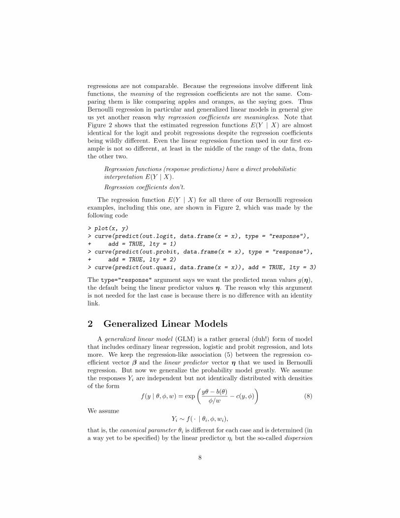
regressions are not comparable. Because the regressions involve different linkfunctions, the meaning of the regression coefficients are not the same. Com-paring them is like comparing apples and oranges, as the saying goes. ThusBernoulli regression in particular and generalized linear models in general giveus yet another reason why regression coefficients are meaningless. Note thatFigure 2 shows that the estimated regression functions E(Y | X) are almostidentical for the logit and probit regressions despite the regression coefficientsbeing wildly different. Even the linear regression function used in our first ex-ample is not so different, at least in the middle of the range of the data, fromthe other two.

Regression functions (response predictions) have a direct probabilisticinterpretation E(Y | X).

Regression coefficients don’t.

The regression function E(Y | X) for all three of our Bernoulli regressionexamples, including this one, are shown in Figure 2, which was made by thefollowing code

> plot(x, y)

> curve(predict(out.logit, data.frame(x = x), type = "response"),

+ add = TRUE, lty = 1)

> curve(predict(out.probit, data.frame(x = x), type = "response"),

+ add = TRUE, lty = 2)

> curve(predict(out.quasi, data.frame(x = x)), add = TRUE, lty = 3)

The type="response" argument says we want the predicted mean values g(η),the default being the linear predictor values η. The reason why this argumentis not needed for the last case is because there is no difference with an identitylink.

2 Generalized Linear Models

A generalized linear model (GLM) is a rather general (duh!) form of modelthat includes ordinary linear regression, logistic and probit regression, and lotsmore. We keep the regression-like association (5) between the regression co-efficient vector β and the linear predictor vector η that we used in Bernoulliregression. But now we generalize the probability model greatly. We assumethe responses Yi are independent but not identically distributed with densitiesof the form

f(y | θ, φ, w) = exp(

yθ − b(θ)φ/w

− c(y, φ))

(8)

We assumeYi ∼ f( · | θi, φ, wi),

that is, the canonical parameter θi is different for each case and is determined (ina way yet to be specified) by the linear predictor ηi but the so-called dispersion

8

●

●

●

● ●

●●● ●●

●●

●

●

● ●●

● ● ●●

●●

● ●

● ●

●●

●

● ●

● ●●

●●

●●

●

●● ●

●●

●

●

●● ●

●

●

● ●

●

● ●

● ●

●●

●●●

●

● ●

●

●●

●●

● ●

●●

●

●●

● ●●● ●●

●

●

●●

● ●●

●

●

●

●

●

● ●

●

30 40 50 60 70 80

0.0

0.2

0.4

0.6

0.8

1.0

x

y

Figure 2: Scatter plot and regression functions for Examples 1.1, 1.2, and 1.3.Solid line: regression function for logistic regression (logit link). Dashed line:regression function for probit regression (probit link). Dotted line: regressionfunction for no-name regression (identity link).

9

parameter φ is the same for all Yi. The weight wi is a known positive constant,not a parameter. Also φ > 0 is assumed (φ < 0 would just change the sign ofsome equations with only trivial effect). The function b is a smooth function butotherwise arbitrary. Given b the function c is determined by the requirementthat f integrate to one (like any other probability density).

The log likelihood is thus

l(β) =n∑

i=1

(yiθi − b(θi)

φ/wi− c(yi, φ)

)(9)

Before we proceed to the likelihood equations, let us first look at what theidentities derived from differentiating under the integral sign

Eθ{l′n(θ)} = 0 (10)

andEθ{l′′n(θ)} = − varθ{l′n(θ)} (11)

and their multiparameter analogs

Eθ{∇ln(θ)} = 0 (12)

andEθ{∇2ln(θ)} = − varθ{∇ln(θ)} (13)

tell us about this model. Note that these identities are exact, not asymptotic,and so can be applied to sample size one and to any parameterization. So letus differentiate one term of (9) with respect to its θ parameter

l(θ, φ) =yθ − b(θ)

φ/w− c(y, φ)

∂l(θ, φ)∂θ

=y − b′(θ)

φ/w

∂2l(θ, φ)∂θ2

= −b′′(θ)φ/w

Applied to this particular situation, the identities from differentiating under theintegral sign are

Eθ,φ

{∂l(θ, φ)

∂θ

}= 0

varθ,φ

{∂l(θ, φ)

∂θ

}= −Eθ,φ

{∂2l(θ, φ)

∂θ2

}or

Eθ,φ

{Y − b′(θ)

φ/w

}= 0

varθ,φ

{Y − b′(θ)

φ/w

}=

b′′(θ)φ/w

10

From which we obtain

Eθ,φ(Y ) = b′(θ) (14a)

varθ,φ(Y ) = b′′(θ)φ

w(14b)

From this we derive the following lemma.

Lemma 1. The function b in (8) has the following properties

(i) b is strictly convex,

(ii) b′ is strictly increasing,

(iii) b′′ is strictly positive,

unless b′′(θ) = 0 for all θ and the distribution of Y is concentrated at one pointfor all parameter values.

Proof. Just by ordinary calculus (iii) implies (ii) implies (i), so we need onlyprove (iii). Equation (14b) and the assumptions φ > 0 and w > 0 implyb′′(θ) ≥ 0. So the only thing left to prove is that if b′′(θ∗) = 0 for any one θ∗,then actually b′′(θ) = 0 for all θ. By (14b) b′′(θ∗) = 0 implies varθ∗,φ(Y ) = 0,so the distribution of Y for the parameter values θ∗ and φ is concentrated atone point. But now we apply a trick using the distribution at θ∗ to calculatefor other θ

f(y | θ, φ, w) =f(y | θ, φ, w)f(y | θ∗, φ, w)

f(y | θ∗, φ, w)

= exp(

yθ − b(θ)φ/wi

− yθ∗ − b(θ∗)φ/wi

)f(y | θ∗, φ, w)

The exponential term is strictly positive, so the only way the distribution of Ycan be concentrated at one point and have variance zero for θ = θ∗ is if thedistribution is concentrated at the same point and hence has variance zero forall other θ. And using (14b) again, this would imply b′′(θ) = 0 for all θ.

The “unless” case in the lemma is uninteresting. We never use probabilitymodels for data having distributions concentrated at one point (that is, constantrandom variables). Thus (i), (ii), and (iii) of the lemma hold for any GLM wewould actually want to use. The most important of these is (ii) for a reasonthat will be explained when we return to the general theory after the followingexample.

Example 2.1 (Binomial Regression).We generalize Bernoulli regression just a bit by allowing more than one Bernoullivariable to go with each predictor value xi. Adding those Bernoullis gives abinomial response, that is, we assume

Yi ∼ Binomial(mi, pi)

11

where mi is the number of Bernoulli variables with predictor vector xi. Thedensity for Yi is

f(yi | pi) =(

mi

yi

)pyi

i (1− pi)mi−yi

we try to match this up with the GLM form. So first we write the density asan exponential

f(yi | pi) = exp[yi log(pi) + (mi − yi) log(1− pi) + log

(mi

yi

)]= exp

[yi log

(pi

1− pi

)+ mi log(1− pi) + log

(mi

yi

)]= exp

{mi

[yiθi − b(θi)

]+ log

(mi

yi

)}where we have defined

yi = yi/mi

θi = logit(pi)b(θi) = − log(1− pi)

So we see that

• The canonical parameter for the binomial model is θ = logit(p). Thatexplains why the logit link is popular.

• The weight wi in the GLM density turns out to be the number of Bernoullismi associated with the i-th predictor value. So we see that the weightallows for grouped data like this.

• There is nothing like a dispersion parameter here. For the binomial familythe dispersion is known; φ = 1.

Returning to the general GLM model (a doubly redundant redundancy), wefirst define yet another parameter, the mean value parameter

µi = Eθi,φ(Yi) = b′(θi).

By (ii) of Lemma 1 b′ is a strictly increasing function, hence an invertible func-tion. Thus the mapping between the canonical parameter θ and the mean valueparameter µ is an invertible change of parameter. Then by definition of “linkfunction” the relation between the mean value parameter µi and the linear pre-dictor ηi is given by the link function

ηi = g(µi).

The link function g is required to be a strictly increasing function, hence aninvertible change of parameter.

12

If, as in logistic regression we take the linear predictor to be the canonicalparameter, that determines the link function, because ηi = θi implies g−1(θ) =b′(θ). In general, as is the case in probit regression, the link function g and thefunction b′ that connects the canonical and mean value parameters are unrelated.

It is traditional in GLM theory to make primary use of the mean valueparameter and not use the canonical parameter (unless it happens to be thesame as the linear predictor). For that reason we want to write the variance asa function of µ rather than θ

varθi,φ(Yi) =φ

wV (µi) (15)

whereV (µ) = b′′(θ) when µ = b′(θ)

This definition of the function V makes sense because the function b′ is aninvertible mapping between mean value and canonical parameters. The functionV is called the variance function even though it is only proportional to thevariance, the complete variance being φV (µ)/w.

2.1 Parameter Estimation

Now we can write out the log likelihood derivatives

∂l(β)∂βj

=n∑

i=1

(yi − b′(θi)

φ/wi

)∂θi

∂βj

=n∑

i=1

(yi − µi

φ/wi

)∂θi

∂βj

In order to completely eliminate θi we need to calculate the partial derivative.First note that

∂µi

∂θi= b′′(θi)

so by the inverse function theorem

∂θi

∂µi=

1b′′(θi)

=1

V (µi)

Now we can write

∂θi

∂βj=

∂θi

∂µi

∂µi

∂ηi

∂ηi

∂βj=

1V (µi)

h′(ηi)xij (16)

where h = g−1 is the inverse link function. And we finally arrive at the likeli-hood equations expressed in terms of the mean value parameter and the linearpredictor

∂l(β)∂βj

=1φ

n∑i=1

(yi − µi

V (µi)

)wih

′(ηi)xij

13

These are the equations the computer sets equal to zero and solves to findthe regression coefficients. Note that the dispersion parameter φ appears onlymultiplicatively. So it cancels when the partial derivatives are set equal tozero. Thus the regression coefficients can be estimated without estimating thedispersion (just as in linear regression).

Also as in linear regression, the dispersion parameter is not estimated bymaximum likelihood but by the method of moments. By (15)

E

{wi(Yi − µi)2

V (µi)

}=

wi

V (µi)var(Yi) = φ

Thus1n

n∑i=1

wi(yi − µi)2

V (µi)

would seem to be an approximately unbiased estimate of φ. Actually it is notbecause µ is not µ, and

φ =1

n− p

n∑i=1

wi(yi − µi)2

V (µi)

is closer to unbiased where p is the rank of the design matrix X. We won’tbother to prove this. The argument is analogous to the reason for n−p in linearregression.

2.2 Fisher Information, Tests and Confidence Intervals

The log likelihood second derivatives are

∂2l(β)∂βj∂βk

=n∑

i=1

(yi − b′(θi)

φ/wi

)∂2θi

∂βj∂βk−

n∑i=1

(b′′(θi)φ/wi

)∂θi

∂βj

∂θi

∂βk

This is rather a mess, but because of (14a) the expectation of the first sum iszero. Thus the j, k term of the expected Fisher information is, using (16) andb′′ = V ,

−E

{∂2l(β)∂βj∂βk

}=

n∑i=1

(b′′(θi)φ/wi

)∂θi

∂βj

∂θi

∂βk

=n∑

i=1

(V (µi)φ/wi

)1

V (µi)h′(ηi)xij

1V (µi)

h′(ηi)xik

=1φ

n∑i=1

(wih

′(ηi)2

V (µi)

)xijxik

We can write this as a matrix equation if we define D to be the diagonal matrixwith i, i element

dii =1φ

wih′(ηi)2

V (µi)

14

ThenI(β) = X′DX

is the expected Fisher information matrix. From this standard errors for theparameter estimates, confidence intervals, test statistics, and so forth can bederived using the usual likelihood theory. Fortunately, we do not have to do allof this by hand. R knows all the formulas and computes them for us.

3 Poisson Regression

The Poisson model is also a GLM. We assume responses

Yi ∼ Poisson(µi)

and connection between the linear predictor and regression coefficients, as al-ways, of the form (5). We only need to identify the link and variance functionsto get going. It turns out that the canonical link function is the log function(left as an exercise for the reader). The Poisson distribution distribution hasthe relation

var(Y ) = E(Y ) = µ

connecting the mean, variance, and mean value parameter. Thus the variancefunction is V (µ) = µ, the dispersion parameter is known (φ = 1), and the weightis also unity (w = 1).

Example 3.1 (Poisson Regression).The data set in the file ex12.10.1.dat is read by


> names(X)

[1] "hour" "count"

> attach(X)

simulates the hourly counts from a not necessarily homogeneous Poisson pro-cess. The variables are hour and count, the first counting hours sequentiallythroughout a 14-day period (running from 1 to 14× 24 = 336) and the secondgiving the count for that hour.

The idea of the regression is to get a handle on the mean as a function oftime if it is not constant. Many time series have a daily cycle. If we pool thecounts for the same hour of the day over the 14 days of the series, we see aclear pattern in the histogram. The R hist function won’t do this, but we canconstruct the histogram ourselves (Figure 3) using barplot with the commands

> hourofday <- (hour - 1)%%24 + 1

> foo <- split(count, hourofday)

> foo <- sapply(foo, sum)

> barplot(foo, space = 0, xlab = "hour of the day", ylab = "total count",

+ names = as.character(1:24), col = 0)

15

1 3 5 7 9 11 13 15 17 19 21 23

hour of the day

tota

l cou

nt

020

4060

8010

012

0

Figure 3: Histogram of the total count in each hour of the day for the data forExample 3.1.

16

In contrast, if we pool the counts for each day of the week, the histogramis fairly even (not shown). Thus it seems to make sense to model the meanfunction as being periodic with period 24 hours, and the obvious way to do thatis to use trigonometric functions. Let us do a bunch of fits

> w <- hour/24 * 2 * pi

> out1 <- glm(count ~ I(sin(w)) + I(cos(w)), family = poisson)

> summary(out1)

Call:glm(formula = count ~ I(sin(w)) + I(cos(w)), family = poisson)


-3.78327 -1.18758 -0.05076 0.86991 3.42492


(Intercept) 1.73272 0.02310 75.02 < 2e-16 ***I(sin(w)) -0.10067 0.03237 -3.11 0.00187 **I(cos(w)) -0.21360 0.03251 -6.57 5.04e-11 ***---Signif. codes: 0 ‘***’ 0.001 ‘**’ 0.01 ‘*’ 0.05 ‘.’ 0.1 ‘ ’ 1

(Dispersion parameter for poisson family taken to be 1)



> out2 <- update(out1, . ~ . + I(sin(2 * w)) + I(cos(2 * w)))

> summary(out2)

Call:glm(formula = count ~ I(sin(w)) + I(cos(w)) + I(sin(2 * w)) +

I(cos(2 * w)), family = poisson)


-3.20425 -0.74314 -0.09048 0.61291 3.26622


(Intercept) 1.65917 0.02494 66.516 < 2e-16 ***I(sin(w)) -0.13916 0.03128 -4.448 8.66e-06 ***

17

I(cos(w)) -0.28510 0.03661 -7.787 6.86e-15 ***I(sin(2 * w)) -0.42974 0.03385 -12.696 < 2e-16 ***I(cos(2 * w)) -0.30846 0.03346 -9.219 < 2e-16 ***---Signif. codes: 0 ‘***’ 0.001 ‘**’ 0.01 ‘*’ 0.05 ‘.’ 0.1 ‘ ’ 1




> out3 <- update(out2, . ~ . + I(sin(3 * w)) + I(cos(3 * w)))

> summary(out3)

Call:glm(formula = count ~ I(sin(w)) + I(cos(w)) + I(sin(2 * w)) +

I(cos(2 * w)) + I(sin(3 * w)) + I(cos(3 * w)), family = poisson)


-3.21035 -0.78122 -0.04986 0.48562 3.18471


(Intercept) 1.655430 0.025152 65.818 < 2e-16 ***I(sin(w)) -0.151196 0.032532 -4.648 3.36e-06 ***I(cos(w)) -0.301336 0.038250 -7.878 3.32e-15 ***I(sin(2 * w)) -0.439789 0.034464 -12.761 < 2e-16 ***I(cos(2 * w)) -0.312843 0.033922 -9.222 < 2e-16 ***I(sin(3 * w)) -0.063440 0.033805 -1.877 0.0606 .I(cos(3 * w)) 0.004311 0.033632 0.128 0.8980---Signif. codes: 0 ‘***’ 0.001 ‘**’ 0.01 ‘*’ 0.05 ‘.’ 0.1 ‘ ’ 1




It seems from the pattern of “stars” that maybe it is time to stop. A clearerindication is given by the so-called analysis of deviance table, “deviance” being

18

another name for the likelihood ratio test statistic (twice the log likelihooddifference between big and small models), which has an asymptotic chi-squaredistribution by standard likelihood theory.

> anova(out1, out2, out3, test = "Chisq")

Analysis of Deviance Table

Model 1: count ~ I(sin(w)) + I(cos(w))Model 2: count ~ I(sin(w)) + I(cos(w)) + I(sin(2 * w)) + I(cos(2 * w))Model 3: count ~ I(sin(w)) + I(cos(w)) + I(sin(2 * w)) + I(cos(2 * w)) +

I(sin(3 * w)) + I(cos(3 * w))Resid. Df Resid. Dev Df Deviance P(>|Chi|)

1 333 651.102 331 399.58 2 251.52 2.412e-553 329 396.03 2 3.55 0.17

The approximate P -value for the likelihood ratio test comparing models 1 and2 is P ≈ 0, which clearly indicates that model 1 should be rejected. Theapproximate P -value for the likelihood ratio test comparing models 2 and 3 isP = 0.17, which fairly clearly indicates that model 2 should be accepted andthat model 3 is unnecessary. P = 0.17 indicates exceedingly weak evidencefavoring the larger model. Thus we choose model 2.

The following code

> plot(hourofday, count, xlab = "hour of the day")

> curve(predict(out2, data.frame(w = x/24 * 2 * pi), type = "response"),

+ add = TRUE)

draws the scatter plot and estimated regression function for model 2 (Figure 4).

I hope all readers are impressed by how magically statistics works in thisexample. A glance at Figure 4 shows

• Poisson regression is obviously doing more or less the right thing,

• there is no way one could put in a sensible regression function withoutusing theoretical statistics. The situation is just too complicated.

4 Overdispersion

So far we have seen only models with unit dispersion parameter (φ = 1). Thissection gives an example with φ 6= 1 so we can see the point of the dispersionparameter.

The reason φ = 1 for binomial regression is that the mean value parameterp = µ determines the variance mp(1 − p) = mµ(1 − µ). Thus the variancefunction is

V (µ) = µ(1− µ) (17)

19

●

●

●

●

●

●

●

●

● ●

●

●

● ●

●

● ●

● ●

●

●

●

●

●

●

●

●

●

●

●

●

●

●

●

●

●

●

●

●

●

●

●

●

●

●

● ●

●

● ●

●

●

●

● ●

●

●

●

●

●

●

●

●

●

●

●

●

●

●

●

●

●

●

●

●

●

● ●

●

●

●

●

●

●

●

●

●

●

●

●

●

●

●

●

●

●

●

●

●

●

●

●

●

●

●

●

●

●

●

●

● ●

●

●

●

●

● ●

●

●

● ●

●

●

●

●

● ●

●

●

●

●

●

●

●

●

●

●

●

●

●

● ●

●

●

●

●

●

●

●

●

●

●

●

●

●

●

●

●

● ●

●

● ●

●

●

●

●

● ●

●

● ●

●

●

●

●

●

●

● ●

● ●

●

●

●

● ●

● ●

● ●

●

●

●

●

●

●

●

●

●

●

●

●

● ●

●

●

●

●

●

●

●

●

●

●

●

● ● ●

●

●

●

●

●

●

●

●

●

●

●

●

●

●

●

●

● ●

●

●

●

● ●

●

● ●

●

●

●

●

●

●

●

●

●

●

●

● ●

●

●

●

●

●

●

●

●

●

●

●

●

●

●

● ●

●

●

●

●

●

●

●

●

●

●

●

●

●

●

●

●

● ●

●

●

●

●

●

●

●

●

●

●

●

●

●

●

● ●

●

●

●

●

●

●

●

●

●

●

● ●

●

●

●

●

●

●

●

●

●

●

●

● ●

●

●

5 10 15 20

05

1015

hour of the day

coun

t

Figure 4: Scatter plot and regression curve for Example 3.1 (Poisson regressionwith log link function). The regression function is trigonometric on the scale ofthe linear predictor with terms up to the frequency 2 per day.

20

and the weights are wi = mi, the sample size for each binomial variable (thiswas worked out in detail in Example 2.1).

But what if the model is wrong? Here is another model. Suppose

Yi | Wi ∼ Binomial(mi,Wi)

where the Wi are IID random variables with mean µ and variance τ2. Then bythe usual rules for conditional probability

E(Yi) = E{E(Yi | Wi)} = E(miWi) = miµ

and

var(Yi) = E{var(Yi | Wi)}+ var{E(Yi | Wi)}= E{miWi(1−Wi)}+ var{miWi}= miµ−miE(W 2

i ) + m2i τ

2

= miµ−mi(τ2 + µ2) + m2i τ

2

= miµ(1− µ) + mi(mi − 1)τ2

This is clearly larger than the formula miµ(1−µ) one would have for the binomialmodel. Since the variance is always larger than one would have under thebinomial model.

So we know that if our response variables Yi are the sum of a random mixtureof Bernoullis rather than IID Bernoullis, we will have overdispersion. But howto model the overdispersion? The GLM model offers a simple solution. Allowfor general φ so we have, defining Y i = Yi/mi

E(Y i) = µi

var(Y i) =φ

miµi(1− µi)

=φ

miV (µi)

where V is the usual binomial variance function (17).

Example 4.1 (Overdispersed Binomial Regression).The data set in the file ex12.11.1.dat is read by


> names(X)

[1] "succ" "fail" "x"

> attach(X)

contains some data for an overdispersed binomial model. The commands

21

> y <- cbind(succ, fail)

> out.binom <- glm(y ~ x, family = binomial)

> summary(out.binom)

Call:glm(formula = y ~ x, family = binomial)


-2.73992 -1.10103 0.02212 1.06517 2.24202


(Intercept) -1.92156 0.35321 -5.44 5.32e-08 ***x 0.07436 0.01229 6.05 1.45e-09 ***---Signif. codes: 0 ‘***’ 0.001 ‘**’ 0.01 ‘*’ 0.05 ‘.’ 0.1 ‘ ’ 1




> out.quasi <- glm(y ~ x, family = quasibinomial)

> summary(out.quasi)

Call:glm(formula = y ~ x, family = quasibinomial)


-2.73992 -1.10103 0.02212 1.06517 2.24202

Coefficients:Estimate Std. Error t value Pr(>|t|)

(Intercept) -1.92156 0.41713 -4.607 3.03e-05 ***x 0.07436 0.01451 5.123 5.30e-06 ***---Signif. codes: 0 ‘***’ 0.001 ‘**’ 0.01 ‘*’ 0.05 ‘.’ 0.1 ‘ ’ 1

(Dispersion parameter for quasibinomial family taken to be 1.394695)

Null deviance: 118.317 on 49 degrees of freedomResidual deviance: 72.476 on 48 degrees of freedom

22

AIC: NA


fit both the binomial model (logit link and φ = 1) and the “quasi-binomial”(logit link again but φ is estimated with the method of moments estimator asexplained in the text). Both models have exactly the same maximum likelihoodregression coefficients, but because the dispersions differ, the standard errors,z-values, and P -values differ.

Your humble author finds this a bit unsatisfactory. If the data are reallyoverdispersed, then the standard errors and so forth from the latter output arethe right ones to use. But since the dispersion was not estimated by maximumlikelihood, there is no likelihood ratio test for comparing the two models. Norcould your author find any other test in a brief examination of the literature.Apparently, if one is worried about overdispersion, one should use the modelthat allows for it. And if not, not. But that’s not the way we operate in therest of statistics. I suppose I need to find out more about overdispersion (thiswas first written three years ago and I still haven’t investigated this further).

23

Generalized Linear Models in R – Geyer - Statistics ﬁnish the speciﬁcation of a...

Documents

Transcript of Generalized Linear Models in R – Geyer - Statistics ﬁnish the speciﬁcation of a...