Generalized Linear Models (GLMs) - Princeton...

Generalized Linear Models (GLMs)

Statistical modeling and analysis of neural dataNEU 560, Spring 2018

Lecture 9

Jonathan Pillow

1

Example 3: unknown neuron

-25 0 250

25

50

75

100

(contrast)

(spi

ke c

ount

)

Be the computational neuroscientist: what model would you use?

2

Example 3: unknown neuron

More general setup:

-25 0 250

25

50

75

100

(contrast)

(spi

ke c

ount

)

for some nonlinear function f

3

Answer: stimulus likelihood function - useful for ML stimulus decoding!

Quick Quiz:

1. as a function of y?

2. as a function of ?

The distribution P(y|x, ) can be considered as a function of y, x, or .

spikes stimulus parameters

Answer: encoding distribution - probability distribution over spike counts

Answer: likelihood function - the probability of the data given model params

3. as a function of x?

What is P(y|x, ) :

4

0 20 40

0

20

40

60

(contrast)

(spi

ke c

ount

)

stimulus decoding likelihood

5

0 20 40

0

20

40

60

(contrast)0 20 40 60

Stimulus likelihood function (for decoding)

(spi

ke c

ount

)What is this?

6

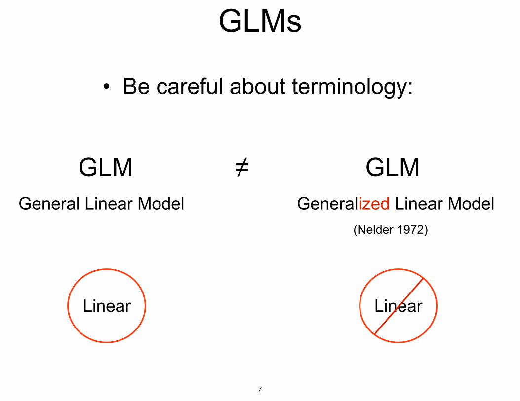
GLMs

• Be careful about terminology:

Linear Linear

General Linear Model Generalized Linear Model

GLM GLM≠

(Nelder 1972)

7

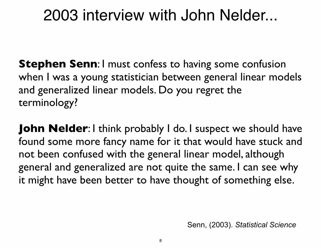
2003 interview with John Nelder...

Stephen Senn: I must confess to having some confusion when I was a young statistician between general linear models and generalized linear models. Do you regret the terminology?

John Nelder: I think probably I do. I suspect we should have found some more fancy name for it that would have stuck and not been confused with the general linear model, although general and generalized are not quite the same. I can see why it might have been better to have thought of something else.

Senn, (2003). Statistical Science

8

Moral:Be careful when naming your model!

9

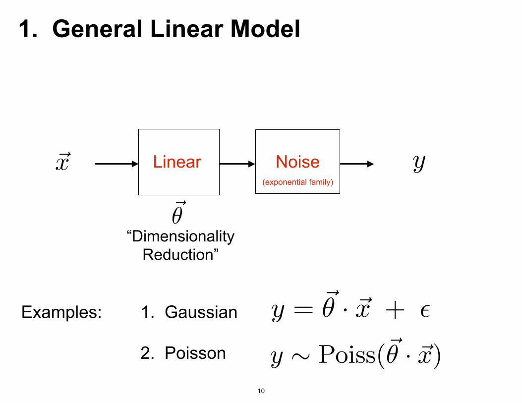
Linear Noise

“Dimensionality Reduction”

(exponential family)

Examples: 1. Gaussian

2. Poisson

y = ~✓ · ~x + ✏

1. General Linear Model

10

2. Generalized Linear Model

Linear

Examples: 1. Gaussian

2. Poisson

Noise(exponential family)

Nonlinear

y = f(~✓ · ~x) + ✏

11

2. Generalized Linear Model

Linear Noise(exponential family)

Nonlinear

Terminology:

“distribution function”

“parameter”= “link function”

12

00 10 00 1 00 0 0 0 0 1 010 10 0 0 0 00 0 0 00 0 00 000 00 0

stimulus

response

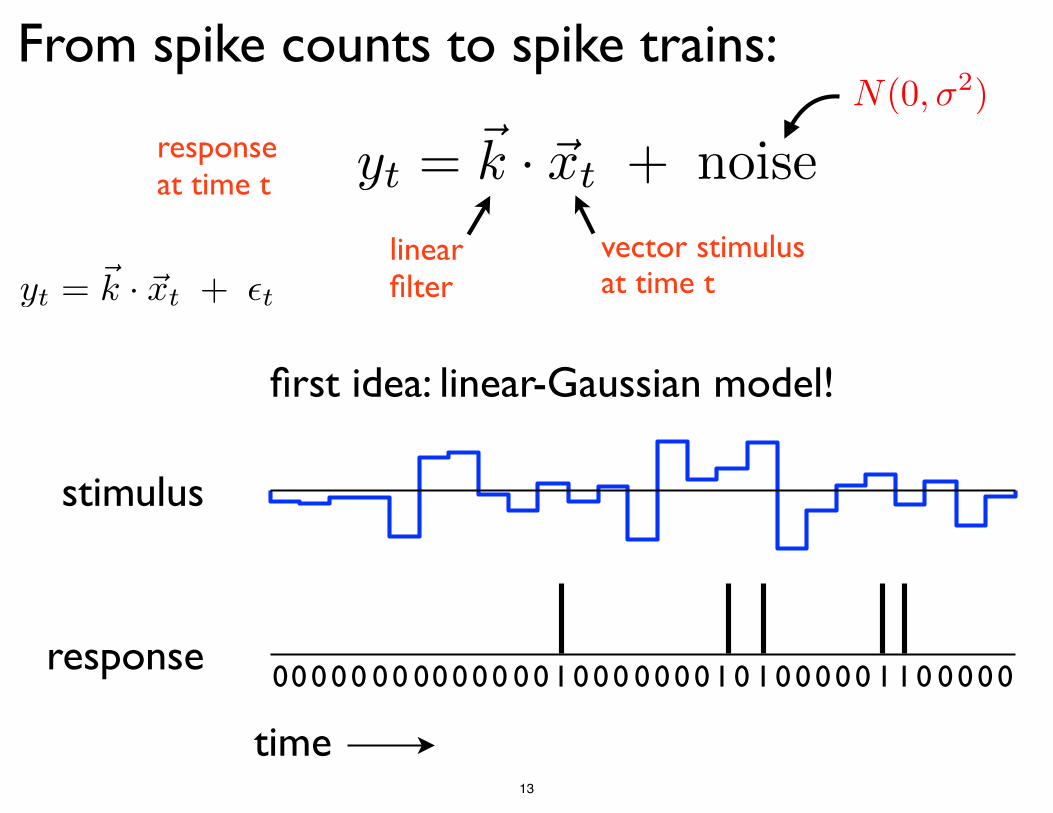
From spike counts to spike trains:

linearfilter

vector stimulus at time t

time

responseat time t

first idea: linear-Gaussian model!

yt = ~k · ~xt + ✏t

yt = ~k · ~xt + noiseN(0,�2)

13

~xt

yt

00 10 00 1 00 0 0 0 0 1 010 10 0 0 0 00 0 0 00 0 00 000 00 0

stimulus

response

linearfilter


yt = ~k · ~xt + noise

time

responseat time t

t = 1

walk through the data one time bin at a time

N(0,�2)

14

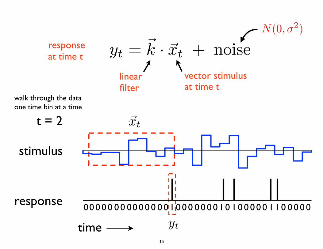
~xt

yt

00 10 00 1 00 0 0 0 0 1 010 10 0 0 0 00 0 0 00 0 00 000 00 0

linearfilter



time

responseat time t

t = 2


stimulus

response

N(0,�2)

15

~xt

yt

00 10 00 1 00 0 0 0 0 1 010 10 0 0 0 00 0 0 00 0 00 000 00 0

linearfilter



time

responseat time t

t = 3


stimulus

response

N(0,�2)

16

~xt

yt

00 10 00 1 00 0 0 0 0 1 010 10 0 0 0 00 0 0 00 0 00 000 00 0

linearfilter



time

responseat time t

t = 4


stimulus

response

N(0,�2)

17

~xt

yt

00 10 00 1 00 0 0 0 0 1 010 10 0 0 0 00 0 0 00 0 00 000 00 0

linearfilter



time

responseat time t

t = 5


stimulus

response

N(0,�2)

18

~xt

yt

00 10 00 1 00 0 0 0 0 1 010 10 0 0 0 00 0 0 00 0 00 000 00 0

linearfilter



time

responseat time t

t = 6


stimulus

response

N(0,�2)

19

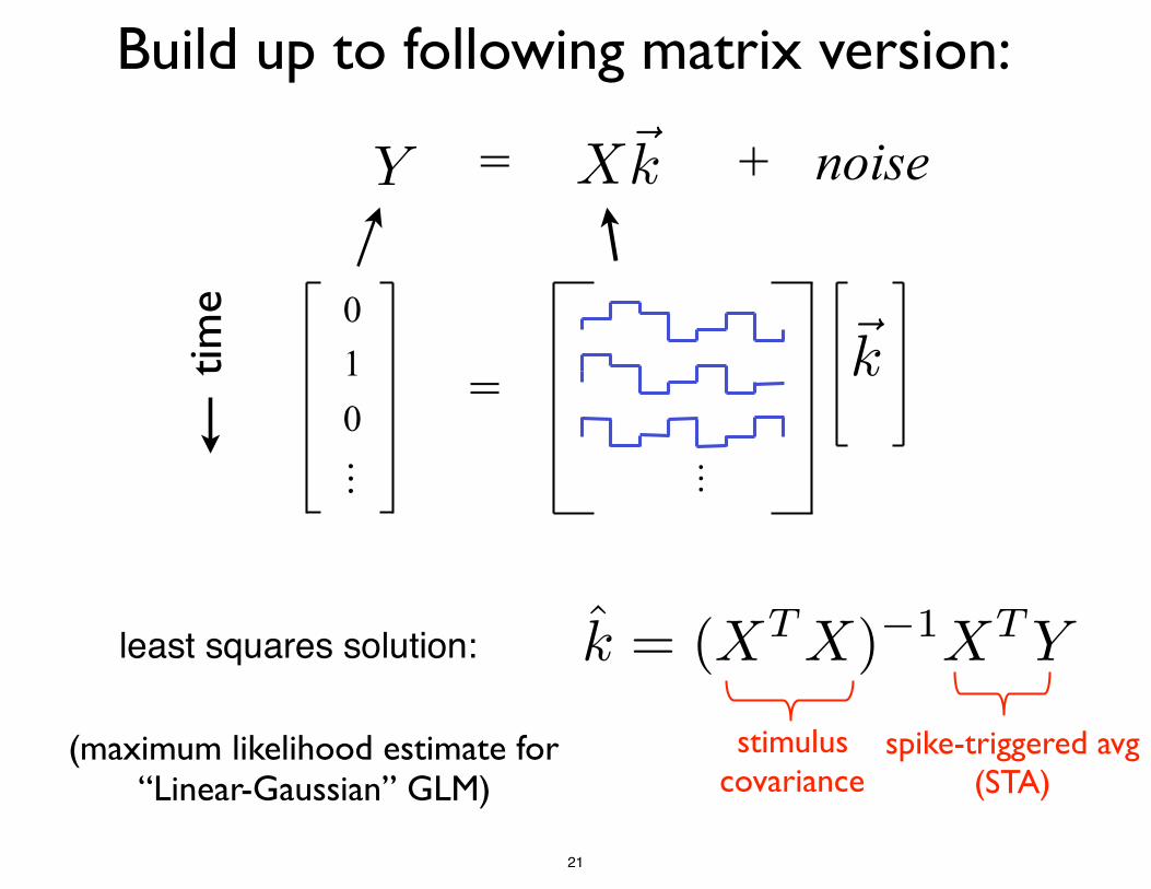
Build up to following matrix version:

0

…

Y X~k= + noise

=time

design matrix

…

~k10

20

Build up to following matrix version:

010

…

Y X~k= + noise

=time

k̂ = (XTX)�1XTY

stimulus covariance

spike-triggered avg(STA)

(maximum likelihood estimate for “Linear-Gaussian” GLM)

least squares solution:

…

~k

21

Formal treatment: scalar version

model:

N(0,�2)

yt = ~k · ~xt + ✏t

equivalent to writing: yt|~xt,~k ⇠ N (~xt · ~k,�2)

p(yt|~xt,~k) =1p

2⇡�2e�

(yt�~xt·~k)2

2�2

or

p(Y |X,~k) =TY

t=1

p(yt|~xt,~k)For entire dataset:(independence

across time bins)

= (2⇡�2)�T2 exp(�

PTt=1

(yt�~xt·~k)22�2 )

Guassian noise with variance �2

logP (Y |X,~k) = �PT

t=1(yt�~xt·~k)2

2�2 + const log-likelihood

22

Formal treatment: vector version

0

…

Y X~k=

…

~k=time

+ ~✏N(0,�2I)

…

+

iid Gaussian noise vector

✏1✏2✏3

equivalent to writing:

orY |X,~k ⇠ N (X~k,�2I)

P (Y |X,~k) = 1

|2⇡�2I|T2exp

⇣� 1

2�2 (Y �X~k)>(Y �X~k)⌘

Take log, differentiate and

set to zero.

10

23

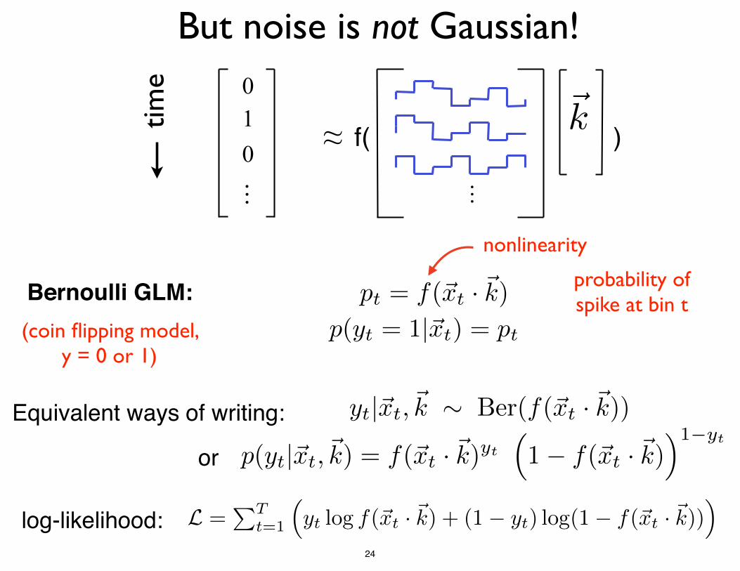
0

… …

~k≈time

probability of spike at bin tBernoulli GLM: pt = f(~xt · ~k)

(coin flipping model, y = 0 or 1)

p(yt = 1|~xt) = pt

nonlinearity

Equivalent ways of writing: yt|~xt,~k ⇠ Ber(f(~xt · ~k))

p(yt|~xt,~k) = f(~xt · ~k)yt

⇣1� f(~xt · ~k)

⌘1�yt

or

But noise is not Gaussian!

log-likelihood: L =PT

t=1

⇣yt log f(~xt · ~k) + (1� yt) log(1� f(~xt · ~k))

⌘

f( )10

24

Logistic regression

Logistic regression: f(x) =1

1 + e�xlogistic function

• so logistic regression is a special case of a Bernoulli GLM

0

… …

~k≈time

probability of spike at bin tBernoulli GLM: pt = f(~xt · ~k)

(coin flipping model, y = 0 or 1)

p(yt = 1|~xt) = pt

nonlinearity

f( )10

25

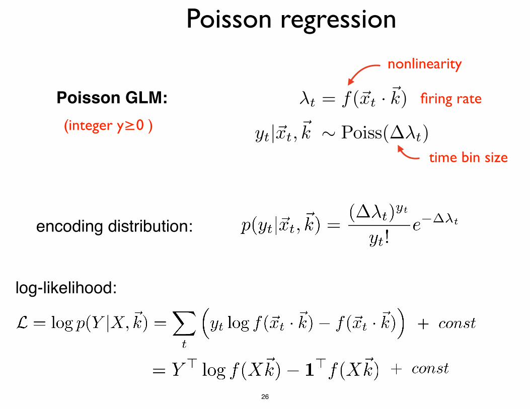
Poisson regression

firing ratePoisson GLM: (integer y≥0 )

nonlinearity

�t = f(~xt · ~k)

yt|~xt,~k ⇠ Poiss(��t)time bin size

<latexit sha1_base64="jbjLJotpTeHkZkaMEURNb7zEwW8=">AAACaXicbVBNb9NAEN2YAm34SssF0ctChJRKEDlcgANSBRw4Va1EaKU4tcbrcbvK7traHYdExv+KPwPXcuyP6Dr1gaaMtKOn997M7r6kUNJRGP7uBHc27t67v7nVffDw0eMnve2d7y4vrcCxyFVuTxJwqKTBMUlSeFJYBJ0oPE5mnxv9eI7Wydx8o2WBUw1nRmZSAHkq7h0Ug2VMP6P5IqbX0Xy2xz/yKLMgqkH0BRUBj5TflkJMe6eVt9Z101/UHE+rN+uWOu71w2G4Kn4bjFrQZ20dxtudjSjNRanRkFDg3GQUFjStwJIUCutuVDosQMzgDCceGtDoptXq4zV/5ZmUZ7n1xxBfsf9OVKCdW+rEOzXQuVvXGvJ/2qSk7P20kqYoCY24vigrFaecNynyVFoUpJYegLDSv5WLc/Cxkc+6240M/hC51mDSyoda+4aCz+o1YdEKiya30XpKt8H47fDDMDwK+/uf2gA32S57yQZsxN6xffaVHbIxE+wX+8Mu2N/OZbATPAueX1uDTjvzlN2ooH8FWym8YQ==</latexit>

log-likelihood:

encoding distribution:

<latexit sha1_base64="QI4yjr0Tf7x9U0q9+/kijSmtHCo=">AAACgXicbVHLThsxFHWGtND0QWiX3VhESKFqowkbWqFKiG666IJKBFJlosjjuZNY8WNk3wmJhvlDfqC/0W27qCfMAgJX8tXxOefK9nGcSeEwDH83gq3ms+fbOy9aL1+9frPb3nt76UxuOQy4kcYOY+ZACg0DFChhmFlgKpZwFc+/VfrVAqwTRl/gKoOxYlMtUsEZemrSTiPFcMaZLH6U9CuNpJnSrPvrZvgxWswPK8blaoJegBS7qzXylrQbLZbVhifG98r6iT7FRlZMZ3g4aXfCXrgu+hj0a9AhdZ1P9hrNKDE8V6CRS+bcqB9mOC6YRcEllK0od5AxPmdTGHmomQI3LtaBlPTAMwlNjfVLI12z9ycKppxbqdg7q+e7Ta0in9JGOaafx4XQWY6g+d1BaS4pGlqlSxNhgaNcecC4Ff6ulM+YZRz9H7RakYZrbpRiOil8PKVvwOm83BCWtbAsfW79zZQeg8FR70sv/Bl2Ts/qAHfIe7JPuqRPjskp+U7OyYBwckv+kL/kX9AMPgRhcHRnDRr1zDvyoIKT/y6qwg4=</latexit>

<latexit sha1_base64="UBowf0owMtkpqKF+vHpz3KYJlks=">AAACYXicbZDPThsxEMadBdp0C21IjwjJaoQEB6LdXtoekBBcOFKJQFA2RF5nNljxn5U9C0SrfQqehis8Re88CE7YQxsYydan7zcjj780l8JhFP1tBCurax8+Nj+Fn9c3vnxtbbbPnSkshx430th+yhxIoaGHAiX0cwtMpRIu0unxnF/cgHXC6DOc5TBUbKJFJjhDb41a+wf0MkGb00SaCc12+8nNdI/u00QxvE6zMq4WtAajVifqRouib0Vciw6p63S02dhOxoYXCjRyyZwbxFGOw5JZFFxCFSaFg5zxKZvAwEvNFLhhufhXRXe8M6aZsf5opAv334mSKedmKvWd83XdMpub77FBgdmvYSl0XiBo/vpQVkiKhs5DomNhgaOcecG4FX5Xyq+ZZRx9lGGYaLjlRimmx6WPpfIXcDqtlsBdDe6WgA+0Kq8SNHnlA42X43srej+6v7vRn6hzeFQn2yRb5DvZJTH5SQ7JCTklPcLJPXkgj+Sp8RyEQStov7YGjXrmG/mvgq0XMHe4Nw==</latexit>

<latexit sha1_base64="WBAIW/X57TGC6zc0oN3xYJP62PU=">AAACPnicbZDLSgNBEEV7fBvfuhShMQiCECZuVNyIblwqGBUyUXo6FW3SL7pr1DDMb7jVX/Ez/AJX4talnTgLjRZ0c7mniipuaqXwGMev0cjo2PjE5NR0ZWZ2bn5hcWn53JvMcWhwI427TJkHKTQ0UKCES+uAqVTCRdo96vOLO3BeGH2GPQstxW606AjOMFjJFk32k33KjfZ4vViNa/Gg6F9RL0WVlHVyvRStJW3DMwUauWTeN+uxxVbOHAouoagkmQfLeJfdQDNIzRT4Vj44uqAbwWnTjnHhaaQD9+dEzpT3PZWGTsXw1g+zvvkfa2bY2W3lQtsMQfPvRZ1MUjS0nwBtCwccZS8Ixp0It1J+yxzjGHKqVBIN99woxXQ7T+66RfiA024xBB5K8DAE0Nkiv0rQ2CIEWh+O769obNf2avFpXD04LJOdIqtknWySOtkhB+SYnJAG4cSSR/JEnqOX6C16jz6+W0eicmaF/Kro8wuQxq9k</latexit>

<latexit sha1_base64="WBAIW/X57TGC6zc0oN3xYJP62PU=">AAACPnicbZDLSgNBEEV7fBvfuhShMQiCECZuVNyIblwqGBUyUXo6FW3SL7pr1DDMb7jVX/Ez/AJX4talnTgLjRZ0c7mniipuaqXwGMev0cjo2PjE5NR0ZWZ2bn5hcWn53JvMcWhwI427TJkHKTQ0UKCES+uAqVTCRdo96vOLO3BeGH2GPQstxW606AjOMFjJFk32k33KjfZ4vViNa/Gg6F9RL0WVlHVyvRStJW3DMwUauWTeN+uxxVbOHAouoagkmQfLeJfdQDNIzRT4Vj44uqAbwWnTjnHhaaQD9+dEzpT3PZWGTsXw1g+zvvkfa2bY2W3lQtsMQfPvRZ1MUjS0nwBtCwccZS8Ixp0It1J+yxzjGHKqVBIN99woxXQ7T+66RfiA024xBB5K8DAE0Nkiv0rQ2CIEWh+O769obNf2avFpXD04LJOdIqtknWySOtkhB+SYnJAG4cSSR/JEnqOX6C16jz6+W0eicmaF/Kro8wuQxq9k</latexit>

26

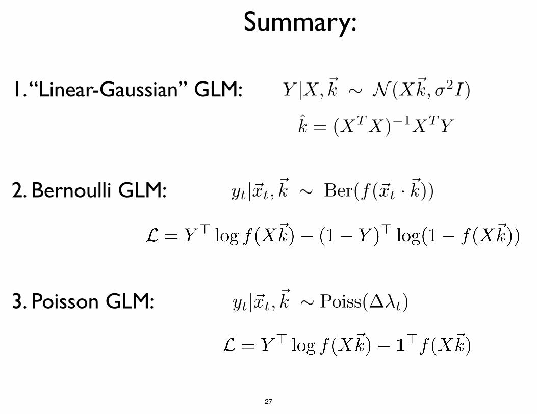
Summary:

k̂ = (XTX)�1XTY

1. “Linear-Gaussian” GLM: Y |X,~k ⇠ N (X~k,�2I)

2. Bernoulli GLM:

3. Poisson GLM: yt|~xt,~k ⇠ Poiss(��t)

yt|~xt,~k ⇠ Ber(f(~xt · ~k))

<latexit sha1_base64="UNt4lEq3y3m8KLk2pIT2tsWpp4c=">AAACbXicbZDNThsxFIWdofw0LRBA6qZQWY0QsCCaYdOyqITaTRcsqERKqkyIPM6dxIp/RvYdSjSaZ+Fpum3XfQseAWeYRQm9kq2j890rX58kk8JhGP5tBEsvlldW1142X71e39hsbW1/dya3HLrcSGN7CXMghYYuCpTQyywwlUi4SqZf5vzqBqwTRl/iLIOBYmMtUsEZemvYOo0Vwwlnsjgv6Sf6I0ab0ViaMU0Pe/HN9Ige06olSYuorGgNhq122Amros9FVIs2qetiuNXYi0eG5wo0csmc60dhhoOCWRRcQtmMcwcZ41M2hr6Xmilwg6L6Y0n3vTOiqbH+aKSV++9EwZRzM5X4zvm6bpHNzf+xfo7px0EhdJYjaP74UJpLiobOA6MjYYGjnHnBuBV+V8onzDKOPtZmM9bwkxulmB4VPpbSX8DptFwAtzW4XQA+0LK4jtFkpQ80WozvueiedE474bewffa5TnaNvCXvySGJyAdyRr6SC9IlnNyRX+Q3+dO4D94Eu8G7x9agUc/skCcVHDwAMYS9SQ==</latexit>

<latexit sha1_base64="HP+VfMMA0E+XGBPwmKdZYtaDvzk=">AAACcnicbZHLahsxFIbl6S11L7GTZSioNQUbGjPTTZJFSkg3WXThQl07eFyjkc84wroM0hknZpi3ydNkm2z6IN1HdgfaOj0g8ev/dJD0K8mkcBiGP2vBo8dPnj7bel5/8fLV6+1Gc+e7M7nl0OdGGjtMmAMpNPRRoIRhZoGpRMIgmX9e8cECrBNGf8NlBmPFZlqkgjP01qTxKVYMLziTxZeSHtPzGG1GY2lmNG0P48W8Q/dpO9o/7/wBflmxDp00WmE3XBd9KKJKtEhVvUmz9iaeGp4r0Mglc24UhRmOC2ZRcAllPc4dZIzP2QxGXmqmwI2L9UNL+t47U5oa64dGunb/7iiYcm6pEr9z9Sy3yVbm/9gox/RwXAid5Qia/z4ozSVFQ1ep0amwwFEuvWDcCn9Xyi+YZRx9tvV6rOGSG6WYnhY+mNJPwOm83ABXFbjaAD7asvgRo8lKH2i0Gd9D0f/YPeqGX8PWyWmV7BbZI+9Im0TkgJyQM9IjfcLJNbkht+Su9ivYC94G1TcEtapnl/xTwYd7gzC9GQ==</latexit>

27

Generalized Linear Models (GLMs) - Princeton...

Documents

Transcript of Generalized Linear Models (GLMs) - Princeton...