GENERALIZED HEEGNER CYCLES,

SHIMURA CURVES, AND SPECIAL VALUES

OF p-ADIC L-FUNCTIONS

by

Ernest Hunter Brooks

A dissertation submitted in partial fulfillmentof the requirements for the degree of

Doctor of Philosophy(Mathematics)

in The University of Michigan2013

Doctoral Committee:

Associate Professor Kartik Prasanna, ChairProfessor Stephen DeBackerProfessor Jeffrey LagariasAssistant Professor Ruochuan LiuProfessor Martin Strauss

ACKNOWLEDGEMENTS

In addition to being a wise and extremely patient advisor, Kartik Prasanna sug-

gested this problem to me and came up with a beautiful idea to treat the case where

wt(f) = 2 and χ gives the trivial character of Gal(H/K), which I had been excluding

in a previous draft. It is impossible to sufficiently thank him. Ruochuan Liu read

a draft of this document and offered several helpful comments. The portion of this

document regarding the construction of Besser’s projector benefitted from conversa-

tions with Kevin Carde and David Speyer. Finally, learning the necessary material

required many conversations with fellow graduate students who did not need to learn

it themselves, among whom I especially thank Ari Shnidman and Julian Rosen.

ii

TABLE OF CONTENTS

ACKNOWLEDGEMENTS . . . . . . . . . . . . . . . . . . . . . . . . . . . . . . . . . . ii

CHAPTER

I. Introduction . . . . . . . . . . . . . . . . . . . . . . . . . . . . . . . . . . . . . . . 1

1.1 The Gross-Zagier formula and its generalizations . . . . . . . . . . . . . . . . 11.1.1 Two consequences of the Heegner hypothesis . . . . . . . . . . . . . 11.1.2 The p-adic Gross-Zagier formula . . . . . . . . . . . . . . . . . . . 41.1.3 Higher-weight modular forms and the geometry of Kuga-Sato va-

rieties . . . . . . . . . . . . . . . . . . . . . . . . . . . . . . . . . . 61.1.4 Higher-weight Hecke characters and a broken symmetry . . . . . . 7

1.2 Removing the Heegner hypothesis . . . . . . . . . . . . . . . . . . . . . . . . 111.2.1 Zhang’s work on Shimura curves . . . . . . . . . . . . . . . . . . . 111.2.2 Main result and sketch of proof . . . . . . . . . . . . . . . . . . . . 131.2.3 Outline of this document . . . . . . . . . . . . . . . . . . . . . . . . 17

II. Shimura curves . . . . . . . . . . . . . . . . . . . . . . . . . . . . . . . . . . . . . 21

2.1 Initial choices . . . . . . . . . . . . . . . . . . . . . . . . . . . . . . . . . . . 212.2 Review of quaternion algebras . . . . . . . . . . . . . . . . . . . . . . . . . . 21

2.2.1 Quaternion Algebras over local fields . . . . . . . . . . . . . . . . . 242.2.2 Quaternion Algebras over Q . . . . . . . . . . . . . . . . . . . . . . 24

2.3 Integral Structures in Quaternion Algebras . . . . . . . . . . . . . . . . . . . 252.3.1 Integrality and Orders . . . . . . . . . . . . . . . . . . . . . . . . . 25

2.4 Review of Shimura curves . . . . . . . . . . . . . . . . . . . . . . . . . . . . . 262.4.1 Shimura Curves, Complex Analytically . . . . . . . . . . . . . . . . 262.4.2 False Elliptic Curves . . . . . . . . . . . . . . . . . . . . . . . . . . 27

2.5 The fixed Shimura curve . . . . . . . . . . . . . . . . . . . . . . . . . . . . . 282.5.1 Arithmetic model . . . . . . . . . . . . . . . . . . . . . . . . . . . . 29

2.6 CM points on Shimura curves . . . . . . . . . . . . . . . . . . . . . . . . . . 302.6.1 Complex uniformization of false elliptic curves and CM points . . . 302.6.2 The action of Cl(K) and Shimura’s reciprocity law . . . . . . . . . 31

2.7 Shimura curves and Kuga-Sato varieties . . . . . . . . . . . . . . . . . . . . . 332.8 The transfer . . . . . . . . . . . . . . . . . . . . . . . . . . . . . . . . . . . . 342.9 Standard cohomology classes . . . . . . . . . . . . . . . . . . . . . . . . . . . 352.10 Assumptions . . . . . . . . . . . . . . . . . . . . . . . . . . . . . . . . . . . . 36

III. Modular forms and p-adic modular forms on Shimura curves . . . . . . . . 38

3.1 Modular forms on Shimura curves . . . . . . . . . . . . . . . . . . . . . . . . 383.1.1 Classical modular forms . . . . . . . . . . . . . . . . . . . . . . . . 383.1.2 p-adic modular forms . . . . . . . . . . . . . . . . . . . . . . . . . . 39

3.2 The Gauss-Manin Connection . . . . . . . . . . . . . . . . . . . . . . . . . . 41

iii

3.2.1 Complex-analytic construction . . . . . . . . . . . . . . . . . . . . 413.2.2 Algebraic construction . . . . . . . . . . . . . . . . . . . . . . . . . 43

3.3 The Kodaira-Spencer Map . . . . . . . . . . . . . . . . . . . . . . . . . . . . 443.4 Katz’s differential operators arising from the Hodge sequence. . . . . . . . . 46

3.4.1 The Maass-Shimura operator Θ∞ . . . . . . . . . . . . . . . . . . . 473.4.2 The Ramanujan-Atkin-Serre operator θ . . . . . . . . . . . . . . . 483.4.3 Coincidence of the operators at CM points . . . . . . . . . . . . . . 49

3.5 Hecke operators and p-adic Hecke operators . . . . . . . . . . . . . . . . . . 49

IV. Serre-Tate coordinates: general theory . . . . . . . . . . . . . . . . . . . . . . 52

4.1 Serre-Tate coordinates . . . . . . . . . . . . . . . . . . . . . . . . . . . . . . 534.2 Katz’s computation of ∇ . . . . . . . . . . . . . . . . . . . . . . . . . . . . . 55

V. Serre-Tate coordinates: the case of Shimura curves . . . . . . . . . . . . . . 59

5.1 Serre-Tate coordinates for Shimura curves . . . . . . . . . . . . . . . . . . . 595.2 The operator θ in coordinates . . . . . . . . . . . . . . . . . . . . . . . . . . 615.3 Hecke operators in coordinates . . . . . . . . . . . . . . . . . . . . . . . . . . 625.4 Continuity properties of the operators . . . . . . . . . . . . . . . . . . . . . . 685.5 Proof of Proposition III.6 . . . . . . . . . . . . . . . . . . . . . . . . . . . . . 70

VI. Twisted cohomology groups and residue theory . . . . . . . . . . . . . . . . . 72

6.1 Review of Deligne’s twisted cohomology groups . . . . . . . . . . . . . . . . 726.2 Residues, algebraically . . . . . . . . . . . . . . . . . . . . . . . . . . . . . . 736.3 Coleman’s rigid analytic theory of residues . . . . . . . . . . . . . . . . . . . 76

VII. Construction of the cycle . . . . . . . . . . . . . . . . . . . . . . . . . . . . . . . 81

7.1 Projectors on Kuga-Sato varieties and the cohomology of Shimura curves . . 817.2 The generalized Heegner cycle and the p-adic Abel-Jacobi map . . . . . . . . 86

7.2.1 The p-adic Abel-Jacobi map . . . . . . . . . . . . . . . . . . . . . . 877.3 The case of weight two . . . . . . . . . . . . . . . . . . . . . . . . . . . . . . 89

VIII. Computation of the p-adic Abel-Jacobi map . . . . . . . . . . . . . . . . . . . 90

8.1 The p-adic Abel-Jacobi map and Coleman integration . . . . . . . . . . . . . 908.2 Computing Coleman primitives for p-adic modular forms . . . . . . . . . . . 92

IX. The p-adic L-function . . . . . . . . . . . . . . . . . . . . . . . . . . . . . . . . . 96

9.1 Spaces of Hecke characters . . . . . . . . . . . . . . . . . . . . . . . . . . . . 969.2 The Waldspurger-type result . . . . . . . . . . . . . . . . . . . . . . . . . . . 97

9.2.1 CM points and CM triples . . . . . . . . . . . . . . . . . . . . . . . 1009.3 The p-adic L-function . . . . . . . . . . . . . . . . . . . . . . . . . . . . . . . 1049.4 Special values of Lp . . . . . . . . . . . . . . . . . . . . . . . . . . . . . . . . 105

BIBLIOGRAPHY . . . . . . . . . . . . . . . . . . . . . . . . . . . . . . . . . . . . . . . . 107

iv

CHAPTER I

Introduction

The theory of special values of L-functions links geometric invariants of algebraic

cycles with values of functions that are defined purely analytically. An important

tool for establishing results toward the many conjectural formulas in this area is

the theory of Heegner points, as exemplified by the seminal work [GZ] of Gross and

Zagier.

1.1 The Gross-Zagier formula and its generalizations

1.1.1 Two consequences of the Heegner hypothesis

Fix a normalized weight two newform f on Γ0(N) with trivial nebentypus and

rational Hecke eigenvalues. Gross and Zagier consider an imaginary quadratic field

K satisfying the so-called

Heegner hypothesis: All primes q dividing N are split or ramified in K;

moreover, if q|N is ramified in K, then q2 - N .

This seemingly technical hypothesis in fact contributes in an essential way to both

the geometric and analytic side of Gross and Zagier’s famous result.

1

2

On the geometric side, the Heegner hypothesis, which is equivalent to the existence

of an ideal N of K whose norm is N , implies the existence of a cyclic degree N -

isogeny of complex elliptic curves

COK−→ CN−1

,

that is, a point on the modular curve X0(N)(C). The classical theory of complex

multiplication implies that this point is actually an H-point of X0(N), where H

denotes the Hilbert class field of K. Writing P ∈ X0(N)(H) for this point (a

“Heegner point”), we may consider its trace

P1 :=∑

σ∈Gal(H/K)

P σ,

or, more generally, for a character χ : Gal(H/K)→ C×, the twisted trace

Pχ :=∑

σ∈Gal(H/K)

χ−1(σ)P σ

(the symbol 1 denotes the trivial character).

Then Pχ is a divisor (with C-coefficients) on X0(N), defined over H, in the χ-

eigenspace for the action of Gal(H/K) of DivH(X0(N)). There is an elliptic curve

E and a modular parametrization

φ : X0(N)→ E

determined by f , normalized so as to map the cusp∞ to the origin. ThenQχ = φ(Pχ)

is a (C-coefficient) divisor Qχ on E, and in particular Q1 ∈ E(K) is a rational point.

On the analytic side, the Heegner hypothesis affects the vanishing behavior of the

Rankin-Selberg L-function L(f, χ, s), where f denotes the newform attached to E.

More precisely, the completed L-function Λ(f, χ, s) has a functional equation of the

form

Λ(f, χ, s) = ε(f, χ, s)Λ(f, χ, 2− s).

3

At the central point s = 1, the factor ε(f, χ, 1) = ±1 is a product of local signs

εv(f, χ), where v ranges over the places of Q. At the “good reduction” places v - N

the sign εv(f, χ) is 1, while the sign at v =∞ is

ε∞(f, χ) = −1,

which one can calculate as a consequence of a comparison of the weight of f (which

is 2) and the weight of χ (which is 0). The Heegner hypothesis forces the local sign

εv(f, χ) to be 1 whenever v|N , and so the global sign ε(f, χ, 1) is −1. Thus the

Heegner hypothesis forces the vanishing of the L-function at s = 1.

Recall that E(K) is equipped with a symmetric real-valued height pairing such

that 〈R,R〉 = 0 if and only if R is a torsion point of E(K). Below, and in the rest of

the introduction, the sign.= indicates that two values are equal up to multiplication

by a nonzero constant that we have omitted for simplicity (in each case, the explicit

constant can be found in the cited reference). The following formula is Theorem I.6.1

of [GZ].

Theorem I.1 (Gross-Zagier). One has

L′(f, χ, 1).= 〈Qχ, Qχ〉.

In the case χ = 1, the Rankin-Selberg L-function coincides with the L-function

L(E/K, 1) of the base change of E to K. If the derivative of this L-function is

nonzero (which implies that the analytic rank of E/K is exactly one), then the

Gross-Zagier formula shows that the rank of E(K) is at least one, confirming an

implication of the Birch and Swinnerton-Dyer conjecture for K. As is explained on

p. 312 of [GZ], this result descends to Q after incorporating a non-vanishing result

of Waldspurger. Waldspurger’s result ([Wa]) shows that one can pick K such that

4

the pair (K,N) satisfies the Heegner hypothesis and the quadratic twist E ′ of E by

the field K satisfies L′(E ′/Q, 1) 6= 0. It then follows from the factorization

L(E/K, s) = L(E/Q, s)L(E ′/Q, s)

and an analysis of the constants in Theorem I.1 that

L′(E/Q, 1).= 〈TrK/QQχ,TrK/QQχ〉.

1.1.2 The p-adic Gross-Zagier formula

A p-adic variation on this theme was discovered by Perrin-Riou quickly following

the announcement of [GZ]. In order to contextualize her work a little better, we

consider an older result of Leopoldt. Consider the Dirichlet L-functions L(s, χ) as

χ varies over Dirichlet characters of Z. The values of L(s, χ) at negative integers

are algebraic. Pick an isomorphism C ' Cp and compatible embeddings Q ⊂ C and

Q ⊂ Cp, and write ω for the C-valued “Teichmuller character” of conductor p, given

by

Z\pZ → Z×p = µp−1 × (1 + pZp)→ µp−1 ⊂ C×p ' C×.

In [KL], Kubota and Leopoldt established the existence of an analytic p-adic L-

function LDirichletp (·, χ), a function from Cp to Cp satisfying the interpolation property

(for n ≥ 0)

LDirichletp (1− n, χ) = (1− χω−n(p)pn−1)L(1− n, χω−n).

(Such a function is necessarily unique.) When χ is an odd character, the p-adic

L-function identically vanishes. On the other hand, when χ is an even character,

Leopoldt established the remarkable formula1

Lp(1, χ) = −(

1− χ(p)

p

)τ(χ)

m

m∑a=1

χ−1(a) logp(1− ζam).

1Leopoldt did not publish this formula; the first published proof is on p. 41 of [Iw].

5

Here, τ(χ) ∈ Q denotes the usual Gauss sum and m denotes the conductor of χ;

the map logp is Iwasawa’s p-adic logarithm and ζm is the image under our chosen

isomorphism of exp(2πim

).

Leopoldt’s formula is striking because it parallels the classical formula

L(1, χ) = −τ(χ)

m

m∑a=1

χ−1(a) log(1− ζam).

This result establishes a fundamental principle: any formula involving special values

of a classical (motivic) L-function should have a p-adic analogue.

Returning to Perrin-Riou’s p-adic variation on Gross-Zagier, suppose that p splits

in K and is prime to N , and write K∞ for the Z2p-extension of K. Then one can view

finite-order Hecke characters of K as p-adic Galois characters of G∞ = Gal(K∞/K).

Still working with a fixed finite-order character χ, Perrin-Riou, using work of Hida,

constructs a p-adic L-function, which we will denote L(1)p (f, χ), on the space of Z×p -

valued characters η of G∞, satisfying an interpolation law of the form

L(1)p (f, χ)(η)

.= L(f, χη, 1), for η a finite order character.

Here the explicit, nonzero constant hidden in the symbol.= includes not only the

Euler factor for L(f, χη, 1) at p as in the Kubota-Leopoldt case, but now also a p-

adic period on the left-hand side, and a complex period on the right. The Heegner

hypothesis and the interpolation law together force

L(1)p (f, χ)(1) = 0.

For a fixed choice ρ of continuous Z×p -valued character ofG∞, we have a “derivative

of Lp in the ρ-direction,” which we denote (hiding the role of ρ) by L(1)′p , given by

the rule

L(1)′

p (f, χ) :=d

dsL(1)p (f, χ)(ρs)|s=0.

6

Perrin-Riou considers the case of ρ the cyclotomic character. She also constructs a

p-adic height pairing 〈 , 〉p, and obtains (Theorem 1.3 of [PR]):

Theorem I.2 (Perrin-Riou). One has

L(1)′

p (f, χ)(1).= 〈Qχ, Qχ〉p.

1.1.3 Higher-weight modular forms and the geometry of Kuga-Sato varieties

Generalizing the Gross-Zagier formula I.1 in a different direction, one can ask for

a formula where now f is allowed to have even weight k ≥ 2 (we still suppose that

f has level N and trivial nebentypus). In this case, the center of the functional

equation is now s = k2, and the analytic theory of the local signs εv(f, χ) does not

change, i.e. the global sign still forces

L(f, χ,k

2) = 0,

and so we expect to be able to express L′(f, χ, k2) in terms of invariants of some

geometric object defined over a number field. Gross and Zagier conjectured in this

case that the appropriate object would be a “Heegner cycle.” To describe these cycles,

we will work for simplicity with X1(N), so that there is a universal (generalized)

elliptic curve E → X1(N). We will also ignore some complications that arise at

cusps of X1(N). Write r = k − 2.The Kuga-Sato variety Wr is defined to be the

r-fold fiber product of E with itself over X1(N) (more accurately, due to problems

above the cusps, it is a canonical desingularization thereof). Modular forms relate

to the cohomology of Wr:

• To say that a holomorphic function f on the upper half plane is a weight k-

modular form is exactly to say that the expression

ωf = f(τ)dτ ∧ dz1 ∧ . . . ∧ dzr

7

gives a well-defined form in Hr+1dR (Wr/C) (here τ is the “horizontal” coordinate

on the upper half plane, and z1, . . . , zr are the standard coordinates on the fibers(C〈1,τ〉

)rof Wr → X1(N).)

• Deligne’s 2-dimensional Galois representation Vf attached to a normalized new-

form f is obtained as a subspace of Hr+1et (Wr,Q`) stable under an action of the

Hecke algebra.

In fact, Scholl has constructed a rank two motive Mf attached to a modular form

f . Its de Rham realization is the space spanned by ωf and its complex conjugate,

and its etale realization is Deligne’s representation Vf (see Theorem 1.2.4 of [Sch]).

These considerations suggest that the correct generalization of the point on a curve

on the geometric side of the Gross-Zagier formula in the higher-weight case should

be algebraic cycles on Wr. In [GZ], Gross and Zagier proposed, for r = 2s, cycles

fibered above a point corresponding to a fixed elliptic curve E with CM by the ring

of integers of K of the form Xs√D

, where

Xs√D

= Γ√D − (E × 0)−D(0 × E),

D is the discriminant of K, and Γ√D denotes the graph of the map [√D] : E → E.

Nekovar [Ne2], borrowing on work of Hida, generalized Perrin-Riou’s p-adic L-

function and p-adic height pairing to this setting, and proved a higher-weight ana-

logue of Theorem I.2. Around the same time, Zhang [Zh1] established the complex

analogue of Theorem I.1 in higher weight.

1.1.4 Higher-weight Hecke characters and a broken symmetry

Each of the formulas we have discussed so far suppose that χ is a finite order

character of Gal(H/K). In [BDP], Bertolini, Darmon, and Prasanna study the case

8

where this assumption is dropped, allowing χ to be a Hecke character of K of weight

less than k.

Consider a Hecke character χ : A×K/K× → C× of K with infinity type a pair of

integers (`1, `2), which means that

χ|(K⊗R)×(z) = z−`1z−`2 .

Then one has χχ = N`1+`2 where N denotes the norm character on ideals. To

match the conventions of [BDP], we work with special values of the Rankin-Selberg

L-function L(f, χ−1, s) rather than L(f, χ, s).

The local sign ε∞(f, χ−1) is no longer forced to be positive, but rather one has

the dichotomy

ε∞(f, χ−1) =

−1, k > |`1 − `2|

1, k ≤ |`1 − `2|

On the other hand, the local signs at finite places do not change (at least under the

assumption that χ is an unramified Hecke character). It follows that the sign of the

global functional equation for L(f, χ−1, s) depends exclusively on the relationship

between k and ` = |`1 − `2|.

Because of this disparity, we say that χ is of type 1 if k > ` and of type 2 if k ≤ `.

One says that χ is critical for f if s = 0 is a critical value for L(f, χ−1, s) in the sense

of Deligne’s conjecture on special values of L-functions, which translates into one of

the following conditions holding:

• (The type 1 case): 1 ≤ `1, `2 ≤ k − 1.

• (The first type 2 case): `1 ≥ k and `2 ≤ 0.

• (The second type 2 case): `1 ≤ 0 and `2 ≥ k.

9

One says χ is central critical if in addition the central character of χ matches the

Nebentypus of f (so that the same Rankin-Selberg L-function shows up on both sides

of the functional equation) and the center of the functional equation for L(f, χ−1, s)

is s = 0. (This latter condition amounts to demanding that `1 + `2 = k.)

Bertolini, Darmon, and Prasanna then construct a p-adic L-function L(2)p (f, )

according to an interpolation law of the form

L(2)p (f, )

.= L(f, χ−1, 0)

where the range of interpolation is the space of central critical characters in the first

type 2 case. Note that these values are not forced a priori to vanish, and therefore

neither are the values

L(2)p (f, χ)

when χ is of type 1 (even though the classical L-function certainly vanishes at these

points). In [BDP], therefore, the values of L(2)p outside the range of interpolation are

investigated, rather than the derivatives.

In the weight two case, their theorem can be stated as follows:

Theorem I.3 (BDP). For χ central critical of type 1, write χ = N · µ where µ is a

finite order character. Then one has

L(2)p (f, χ)

.= logp(Qµ)2

Here logp is the p-adic logarithm on E(Cp), which is the unique locally analytic

primitive F on E(Cp) for the standard Neron differential ω on E such that

F : E(Cp)→ Cp

is a homomorphism of groups.

10

In the higher-weight case, which is also covered in [BDP], the relevant cycles are

no longer Heegner cycles on Kuga-Sato varieties, the point being that the motive

attached to a positive-weight unramified Hecke character of K lives naturally in a

self-product of an elliptic curve E with CM by OK . One must therefore work with

the enlarged variety Wr × Er.

The relevant generalized Heegner cycles are (r-fold products of) graphs of cyclic

degree N -isogenies E → E ′, again supported in a fiber of Wr × Er over a Heegner

point of X1(N), modified by an idempotent designed to render them cohomologically

trivial.

On the analytic side, in higher weight, the p-adic logarithm generalizes to a p-adic

Abel-Jacobi map, which is defined precisely in Section 3.4 of [BDP] or Section 7.2.1

of this document. Write Sk(Qp) for the space of cusp forms of level N and trivial

Nebentypus, defined over Qp.

The p-adic Abel-Jacobi map may be viewed as a map from the space CHr+10 (Wr×

Er) of cohomologically trivial codimension-(r + 1) cycles on Wr × Er to the space

(Sk(Γ0(N),Qp)⊗ SymrH1dR(EQp ,Qp))

∨

of functionals on a piece of the cohomology of the base change of Wr × Er to Qp.

We mention two applications of Theorem I.3. Recent work of Skinner ([Sk])

establishes a converse to Gross-Zagier’s work on the Birch-Swinnerton-Dyer conjec-

ture: Skinner shows that if X(E/Q) is finite and its Mordell-Weil rank is one, then

ords=1L(E, s) = 1. Skinner shows this by using an Iwasawa-theoretic argument of

Xin Wan to establish that, for some choice of K, L(2)p (f,1) 6= 0. It follows from The-

orem I.3 that the logarithm of Qχ is not zero, so Qχ is non-torsion. It then follows

from the original Gross-Zagier formula (Theorem I.1) that L′(E, 1) 6= 0. In another,

purely geometric application, in [BDP2], Bertolini, Darmon, and Prasanna relate

11

the p-adic Abel-Jacobi map to the coniveau filtration on the group CH∗0(Wr × Er),

and as a corollary construct examples where the generalized Heegner cycles are non-

torsion in the Griffiths group of homologically trivial cycles modulo algebraically

trivial cycles.

1.2 Removing the Heegner hypothesis

In this dissertation, we study the situation of [BDP] after dropping the Heegner

hypothesis. Before describing the main results, it is necessary to review results of

Zhang [Zh2] on the Gross-Zagier formula in this setting. We assume for the remainder

of this section that N is prime to the discriminant of K.

1.2.1 Zhang’s work on Shimura curves

Factor

N = N+N−,

where N− is the product of the primes dividing N which remain inert in K. A prime

v dividing N− has local sign εv(f, χ) = −1, so in order to preserve the global sign of

the functional equation, Zhang assumes an even number of primes divide N− (else

there is no Gross-Zagier-type result to be proved.)

For simplicity, assume also that N is squarefree. Write B for the quaternion

algebra over Q with discriminant N−. It is an indefinite quaternion algebra, which

means there is an isomorphism ι∞ : B ⊗ R ∼→ M2(R), because an even number of

primes divide N−. Fix a maximal order OB of B. Let OB,N+ denote an Eichler

order of level N+ in OB (see section 2.3.1); write ΓB,N+ for the group of norm one

elements of this order.

The Riemann surface

H/ΓB,N+

12

is a Shimura curve. So long as N− 6= 1 (in which case this Riemann surface is just

a modular curve), it is already compact.

Unsurprisingly, the Shimura curve has a moduli-theoretic interpretation; it is a

coarse moduli space for principally polarized abelian surfaces A with an embedding

OB → End(A) and a certain type of level structure which depends on N+ (defined

in Section 2.5.1). Such a surface is often called a “false elliptic curve.” To the point

τ ∈ H, one attaches the complex torus

Aτ =C2

ι∞(OB)

τ1

.

together with the natural embedding of OB into its endomorphism ring (this torus

comes with a canonical principal polarization).

The Shimura curve has a model X over Q, which is a coarse moduli space for false

elliptic curves with level structure. The analogues of Heegner points on modular

curves are points in X(H) first studied by Shimura. To define them, note that,

because primes dividing N− are inert in K and primes dividing N+ are split in K,

there is an embedding

ιK : K → B

such that OB,N+ ∩ ιK(K) = ιK(OK). For such an embedding, there is a unique point

τ ∈ H fixed under the action of ι∞(ιK(K×)) ⊂ M2(R). A fundamental theorem of

Shimura shows that the image of τ under the uniformization map H → H/ΓB,N+

is defined over H (see p. 58 of [Sh]). Write P for this Heegner point, and for a

character χ ∈ Gal(H/K), again write

Pχ =∑

σ∈Gal(H/K)

χ−1(σ)P σ.

13

For simplicity, suppose χ 6= 1, so that the divisor Pχ has degree zero and therefore

it makes sense to write Qχ for the image of Pχ in Div0(E).

Using the height pairing 〈 , 〉 on Af , Zhang then shows the following (Theorem

C of [Zh2]):

Theorem I.4 (Zhang). For f of weight 2, one has

L(f, χ, 1).= 〈Pχ, Pχ〉

Critical in Zhang’s proof is the Jacquet-Langlands correspondence, which, given

the modular form f (which comes from the classical modular curve of level N),

provides a modular form fB for ΓB,N+ with the same Hecke eigenvalues.

In related work, Disegni ([Di]) has recently established a p-adic analogue of

Theorem I.4; that is to say, he has removed the Heegner hypothesis from Perrin-

Riou’s Theorem I.2, relating an extension of Perrin-Riou’s p-adic L-function to p-adic

heights of CM points on Shimura curves. Both Zhang and Disegni’s work also treat

the more complicated case of Hilbert modular forms of parallel weight 2, where Q is

replaced by a totally real field (and B is replaced by a quaternion algebra over this

field).

1.2.2 Main result and sketch of proof

In this document, we ask what happens to the p-adic L-function of [BDP] when

the Heegner hypothesis is removed. We work with modular forms f of even weight

2r+2. Writing A for the universal abelian surface over the Shimura curve X and Ar

for its r-fold fiber product over X, the above discussion suggests that there should

be a cycle on Ar × Ar, where A is a fixed false elliptic curve with CM by OK ,

whose image under the p-adic Abel-Jacobi map computes special values of a p-adic

L-function.

14

Write F for a number field containing the ring class field of K mod N+. There is

an idempotent e in B ⊗K selected in Section 2.7, and we state our results below in

terms of the cohomology group eH1dR(A). (If the class number of K is odd, one can

arrange for the fixed surface A to be a self-product E × E of CM elliptic curves, in

which case eH1dR(A) = H1

dR(E).)

We then show the following:

Theorem I.5. Suppose that f has even weight k = 2r + 2, with r ≥ 0, and χ is

an unramified Hecke character of K of infinity type (`1, `2) with `1 + `2 = k and

`1, `2 ≥ 1, so that (`1, `2) = (k − 1 − j, 1 + j) with 0 ≤ j ≤ 2r. Then there is, for

each a ∈ Cl(OK), an algebraic cycle ∆r(a) on

Xr := Ar × Ar,

that is homologically trivial and defined over H, such that

(1.1)Lp(f, χ)

Ω4r−4jp

= Ep(f, χ) ·

∑[a]∈Cl(OK)

χ−1(a) · AJp(∆r(a))(ωfB ∧ ωjAη

2r−jA )

2

,

where

• AJp is the p-adic Abel-Jacobi map, viewed as a map

CH2r+10 (Xr/Fp)→ (Sk(Fp)⊗ Sym2r eH1

dR(A/Fp))∨

with Fp being the completion of F at the chosen prime above p and Sk(Fp) the

space of modular forms of weight k over Fp.

• Ep(f, χ) is the Euler factor of L(f, χ−1, s) evaluated at 0, and Ωp is a p-adic

period attached to A.

• fB is the (suitably-normalized) Jacquet-Langlands lift of f to C, ωfB is the

associated differential form on Ar, and ωA, ηA are a basis for eH1dR(A/H),

15

with ωA holomorphic on A(C) and ηA antiholomorphic on A(C), normalized

such that the cup product 〈ωA, ηA〉 = 1.

The main difficulty in proving Theorem I.5 is in making explicit computations with

modular forms over Shimura curves. Because the groups ΓB,N+ contain no translation

matrices, a modular form on a Shimura curve does not have a q-expansion. While

this makes the technical theory of Shimura curves easier in a few places (for instance,

one has to worry about the integral structure of the fibers over the Kuga-Sato variety

over the cusps in the classical case and not in the Shimura curve case), it also makes

explicit calculation of Hecke operators and other operators on Shimura curves more

challenging. To replace q-expansions, we use so-called Serre-Tate expansions, which

are p-adic expansions of modular forms at CM points coming from the deformation

theory of ordinary abelian varieties in characteristic p. We will give an explicit

description (in Chapter V) for some differential operators and Hecke operators in

terms of these expansions, following work of Brakocevic [Br] and Mori [Mo], then

apply those formulas to establish Theorem I.5.

Before explaining these formulas in a little more detail, we summarize the proof

of the main theorem of [BDP]. In [BDP], a generalized Heegner cycle is built as

described above, then modified by an algebraic projector, due to Scholl, designed

to project the cohomology of the expanded Kuga-Sato variety Wr × Er onto the

subspace

Sr+2(Γ1(N))⊗ SymrH1(E).

Write Υ for their cycle. They compute the image of Υ under the p-adic Abel-Jacobi

map in two steps. The first step is to relate this image to a “Coleman primitive” for

the section of a line bundle on X1(N) attached to f . The second is to compute the

Coleman primitive of f in terms of θ−1f , where θ = q ddq

is the Atkin-Serre p-adic

16

differential operator which maps the space of p-adic modular forms of weight k to

the space of p-adic modular forms of weight k+2. (In simple language, step one says

that the p-adic Abel-Jacobi map is a p-adic integral, and step two says that one can

evaluate this integral by undoing a derivative!) The values of θf coincide with the

values of Θ∞f at CM points, where Θ∞ denotes the Maass-Shimura operator

1

2πi

(d

dτ+

k

z − z

).

The p-adic L-function is then constructed (and computed) using a Waldspurger-type

result expressing values of the classical Rankin-Selberg L-function in terms of values

of Θj∞f at CM points.

We now explain our proof. Our cycle starts life as the 2r-fold power of the

graph of an isogeny from the fixed elliptic curve E to some quotient E ′ (that is,

as an isogeny Ar → (A′)r of “CM false elliptic curves”). It must be modified by

an algebraic projector to be made homologically trivial. When k > 2, we use a

projector originally constructed by Besser, which projects the cohomology of the

expanded Kuga-Sato variety Ar × Ar onto the subspace

M2r+2(ΓB,N+)⊗ Sym2rH1(A).

When k = 2, we instead use a projector that depends on f , namely, the standard

projector, built from Hecke correspondences, cutting out the motive of f (see Section

7.3 for more details). (If χ induces a non-trivial character of Gal(H/K), we could take

the same cycle Qχ as above; the problem is that when χ gives the trivial character,

this cycle is not homologically trivial. This differs from Zhang’s solution to the

similar problem that arises in [Zh2].)

We then evaluate the p-adic Abel-Jacobi map on the image of this cycle. The

proof that the Abel-Jacobi map can be expressed in terms of a Coleman primitive

17

closely follow [BDP]. However, the methods of [BDP] break down in inverting the

differential operator θ, since that paper makes essential use of q-expansions. In

fact, the Atkin-Serre formula for θ above does not even make sense over Shimura

curves, but thanks to Katz, there is a moduli-theoretic interpretation of θ for PEL

Shimura varieties over p-adic fields. To invert θ as an operator, we work in Serre-Tate

coordinates, which are convergent expansions for modular forms on ordinary residue

disks of X. We give formulas for θ−1f on these expansions. As in [BDP], the p-adic

L-function is then constructed (and computed) using a Waldspurger-type result.

Under the hypothesis that p|N− exactly once, Marc Masdeu [Ma] has proven a

similar result by using a p-adic analytic uniformization of the corresponding Shimura

curve, which has bad reduction at p. Such a uniformization, however, is not available

in the case of good reduction. Conversely, our techniques rely heavily on the good

reduction of the Shimura curve, and thus do not recover Masdeu’s results.

1.2.3 Outline of this document

In Chapter II, which is expository in nature, we give a review of the theory of

quaternion algebras over Q and the geometry of the associated Shimura curves. As

explained above, Shimura curves are moduli spaces for false elliptic curves, and in the

second half of this chapter, we also quote the results about false elliptic curves that we

need. The reader who is already familiar with the basic theory of quaternion algebras

may wish to skip the first half of this chapter. We then introduce the notation that

we work with for most of the document, and outline the running assumptions of the

document.

In Chapter III, we discuss the theory of modular forms on Shimura curves, defining

the p-adic differential operator θ and its real analogue Θ∞ discussed above, and we

18

define some Hecke operators. The differential operators in question arise from the

Gauss-Manin connection on the relative cohomology bundle of the universal false

elliptic curve over the Shimura curve, and so we begin Chapter III with a review of

this connection and the related Kodaira-Spencer map. We also use this interpretation

of the differential operator to explain why the Atkin-Serre operator coincides with the

Maass-Shimura operator (for values at CM points), a result originally due to Katz.

Because ordinary false elliptic curves over p-adic fields have “canonical subgroups”

killed by p (as do honest ordinary elliptic curves), the Hecke operator Tp splits into

two pieces V and U . In the classical theory this can be seen already on the level of q-

expansions. We state a commutation relation between the operator θ and the Hecke

operators, although we defer its proof until we have built the necessary machinery.

In Chapters IV and V, we compute the differential operators of Chapter III in

terms of expansions of modular forms at ordinary CM points. To do this, we first

review Serre-Tate theory, which we will use to get an expansion for a modular form

at an ordinary CM point that works as a substitute for a q-expansion. Serre-Tate

theory gives us, on the one-hand, an explicit uniformizer in the ring of rigid analytic

functions on a disk of the Shimura curve containing an ordinary CM point, and on

the other hand, an explicit trivialization of the bundle of p-adic modular forms of

weight k over this disk. We can thus use it to express any modular form locally “in

coordinates,” and we can ask what Hecke operators and differential operators do to

these coordinates. Chapter IV reviews Serre-Tate theory in the general setting, and

Chapter V performs the necessary calculations in the Shimura curve setting. The

main results of these chapters are formulas for Hecke operators in these coordinates,

and a proof that the Atkin-Serre operator is invertible on the space of “prime to p”

p-adic modular forms. (A modular form is prime to p if it is fixed by the idempotent

19

p-adic Hecke operator 1− UV , as defined in Section 3.5. A classical p-adic modular

form is “prime to p” if and only if all its Fourier coefficients of the form anp vanish.)

In Chapter VI, we review residue theory on vector bundles with flat connec-

tions, and Coleman’s p-adic methods for computing these residues. Although these

methods are only used in Chapter VIII, the language of residue theory provides the

motivation for the cycles constructed in Chapter VII.

In Chapter VII, we produce a homologically trivial cycle on a Kuga-Sato variety

over the Shimura curve. The key input here in the higher weight case is work of

Besser, which gives an algebraic projector P taking the cohomology of the Kuga-

Sato variety to the space of quaternionic modular forms. In weight two, the cycle,

in the case of non-trivial characters χ of Gal(H/K), can be taken as a weighted sum

of Heegner points similar to Zhang’s above; however, a uniform treatment which

covers both the trivial and non-trivial character alike, and which is entirely due to

Prasanna, is explained at the end of this chapter. In this chapter, we also define the

p-adic Abel-Jacobi map.

In Chapter VIII, we follow [BDP] closely in interpreting the p-adic Abel-Jacobi

map as a Coleman integral. We then use our formulas from Chapter V to compute

the image of our cycle under the p-adic Abel-Jacobi map.

In Chapter IX, which is the analytic side of this document, we use these for-

mulas and a Waldspurger-type result of Prasanna to build a p-adic L-function (the

construction of which is originally due to Hida), then establish Theorem I.5. The

argument, which is similar to that of [BDP], goes as follows: Prasanna’s formula

gives, for certain CM points Pa, the relation

L(f, χ−1, 0).=

∣∣∣∣∣∣∑

a∈Cl(OK)

χ−1(a)Na−j · (Θj∞f)(Pa)

∣∣∣∣∣∣2

.

20

As mentioned earlier, Θ∞f and θf give the same value when evaluated at CM points.

One can remove the absolute value signs from the Waldspurger formula (at the

expense of introducing a new non-zero constant), and thus one can read the result

as a p-adic formula expressed purely in terms of p-adic differential operators. This

p-adic statement allows us to define the p-adic L-function on the space of type two

Hecke characters, and gives a formula which self-evidently extends by continuity to

the space of type one central critical Hecke characters.

CHAPTER II

Shimura curves

2.1 Initial choices

Fix an odd prime p, an isomorphism C ∼→ Cp, and compatible embeddings of Q

into C and Cp. Fix also a newform fGL2 of level N , with p - N , of nebentypus εf ,

and of even weight k = 2r + 2 (with r ≥ 0).

Let K be an imaginary quadratic field in which (p) = pp splits. Factor N =

N+N−, where primes dividing N− are inert in K, and primes dividing N+ are split

or ramified in K. If a prime divides both N and the discriminant of K, assume also

that it divides N exactly once (in other words, K satisfies the Heegner hypothesis

with respect to the level N+). Assume also that N− is squarefree and divisible by

an even number of primes.

Finally, choose a number field F containing the ring class field of K mod N+

and the Hecke eigenvalues of F . This will be the field of definition of the arithmetic

cycles constructed in this paper.

2.2 Review of quaternion algebras

This section reviews the general theory of quaternion algebras. The reader who is

sufficiently acquainted with this theory to be comfortable with Section 2.5 should skip

to Section 2.4. Let F be a field. A quaternion algebra B over F is a four-dimensional

21

22

central simple algebra over F ; thus it is an F -algebra with center exactly F and no

non-trivial two-sided ideals. Two standard results on central simple algebras will be

useful:

Theorem II.1 (Wedderburn’s Theorem). Any central simple algebra is isomorphic

to a matrix ring over a division algebra D (a division algebra is an F -algebra in

which all nonzero elements are invertible).

Theorem II.2 (The Noether-Skolem Theorem). Let A be a simple F -algebra and

B a central simple F -algebra. If f, g are two homomorphisms from A to B, there is

an element x ∈ B× such that, for any a ∈ A, we have

f(a) = x−1g(a)x.

In particular, any automorphism of a central simple algebra is given by conjugation

by an invertible element.

Now suppose that B is a quaternion algebra. By Wedderburn’s theorem and a

count of F -dimension, we see that B is either a division algebra or is isomorphic to

M2(F ).

If the characteristic of F is not 2, all quaternion algebras arise as follows: let

x, y ∈ F . The symbol (x, y|F ) denotes the four-dimensional vector space on a basis

1, i, j, k together with the multiplication rules i2 = x, j2 = y, ij = −ji = k. For any

field F , the quaternion algebra (1, 1|F ) is the trivial quaternion algebra M2(F ). To

see this, it suffices to find two anticommuting matrices Mi,Mj whose squares are the

identity matrix; one choice is given by

Mi =

1 0

0 −1

Mj =

0 1

1 0

.

23

Further, if x′ = α2x and y′ = β2y, then (x′, y′|F )∼→ (x, y|F ); the isomorphism is

given by i 7→ αi, j 7→ βj.

Definition II.3. A pure quaternion is an element of the subset of B consisting of

0, together with elements of B \ F whose squares lie in F .

This subset, denoted Bpure, is actually a subspace: one checks that in the quater-

nion algebra (a, b|F ), the set of pure quaternions is the F -span of i, j, k.

Thus there is a decomposition of the underlying F -vector space of B

B = F ⊕Bpure.

Consider the vector space automorphism b 7→ b of B acting as 1 on F and −1 on

Bpure, known as the “main involution.” The reduced trace Tr is the additive map

B → F given by

Tr(b) = b+ b,

and the reduced norm Nr is the map B → F given by

N(b) = bb

Note that the main involution satisfies

b1b2 = b2b1,

which shows that N lands in F (which is the subspace fixed by the main involution)

and that N is multiplicative. One usually just speaks of the “trace” and “norm” of

an element of B when there is no risk of confusing them with the trace or norm of

that element acting on B by left-multiplication.

If β 6= 0 ∈ B has norm zero, then it is a zero-divisor and B is not a division ring.

Conversely, if β does not have norm zero, then βσ/N(β) is a multiplicative inverse

24

for β; thus, a quaternion algebra B is a division algebra if and only if there are no

elements of norm zero. This observation links quaternion algebras with quadratic

forms: after writing B = (a, b|F ), there are any elements x+yi+zj+wk of norm zero

if and only if there are any solutions over F to the quadratic form in four variables

given by

x2 − ay2 − bz2 + abw2 = 0.

We now describe the structure of quaternion algebras over local fields and Q.

2.2.1 Quaternion Algebras over local fields

There are two quaternion algebras over R: the two-by-two matrix ring M2(R) and

Hamilton’s quaternions H = (−1,−1|R).

Let Lπ be a finite extension of Qp with uniformizer π. Then, as in the real case,

there are two isomorphism classes of quaternion algebras over Lπ. They are the

trivial quaternion algebra and (π, u|Lπ), where π is a uniformizer and u ∈ OLπ×

is a non-square. This latter algebra always splits (becomes isomorphic to a matrix

algebra) over the unramified extension of degree 2 of Lπ.

2.2.2 Quaternion Algebras over Q

Now suppose that B is a quaternion algebra over Q. The Hasse principle for the

reduced norm form then implies that B is the trivial quaternion algebra if and only

if B ⊗ L is the trivial quaternion algebra for each completion L of Q.

One says that B ramifies at a place v of Q if B ⊗ Qv is a division algebra. The

cardinality of the set of places (possibly including ∞) at which B ramifies is finite

and even. The product ∆ of the finite places at which B ramifies is called the

discriminant of B. Given a squarefree positive integer ∆, there exists a quaternion

algebra of discriminant ∆.

25

One calls a quaternion algebra definite if it ramifies at the Archimedean place

and indefinite otherwise. Thus a quaternion algebra is definite if and only if its

discriminant is divisible by an odd number of distinct primes. If L/Q is an imaginary

quadratic field extension, then B splits over L if and only if every prime that ramifies

in B remains inert in L.

2.3 Integral Structures in Quaternion Algebras

2.3.1 Integrality and Orders

Let O be a subring of L. An O-order in a quaternion algebra is a subring which is

finitely generated as an O-module. Over global and (non-archimedean) local fields,

we will take O the ring of integers, and hence say “order” without reference to O.

An order is maximal if it is not strictly contained in a larger order.

An element α in a quaternion algebra B is said to be O-integral if it satisfies

a monic polynomial with coefficients in O; equivalently, if its “reduced minimal

polynomial”

f(x) = (x− α)(x− ασ) = x2 − Tr(α)x+N(α)

has coefficients in O; equivalently, if O[α] is a finitely generated O-submodule of B.

It is clear from this last description that any order in B must consist exclusively

of integral elements. In fact, any integral element is contained in a maximal order.

If L is a non-archimedean local field, and B/L is the trivial quaternion algebra, then

all maximal orders are conjugate to M2(OL). If B/L is the non-trivial quaternion

algebra, then the set of all integral elements of B form a subring which is the unique

maximal order. To give an order in a quaternion algebra over a global field, it is

necessary and sufficient to give orders in each non-archimedean completion which

are maximal at all but finitely many places.

26

An order in a quaternion algebra is an Eichler order if it is the intersection of two

maximal orders. The “standard Eichler order of level πn” in the trivial quaternion

algebra over a local field Lπ with uniformizer π is a b

πnc d

|a, b, c, d ∈ OLπ .

For any Eichler order O in M2(Lπ), there is some N such that O is conjugate to the

standard Eichler order of level πn.

If B is an indefinite quaternion algebra over Q, then all maximal orders of B are

conjugate. If N is an integer prime to the discriminant of B, and OB is a fixed

maximal order, then we say an order ON ⊂ OB is an Eichler order of level N if its

completion at each place p dividing N is conjugate to the standard Eichler order of

level pvp(N) and its completion at each place p dividing ∆ is the maximal order. Any

two Eichler orders of level N are conjugate.

2.4 Review of Shimura curves

2.4.1 Shimura Curves, Complex Analytically

Write H for the upper half plane. Let B be an indefinite quaternion algebra over

Q with discriminant ∆, and fix an isomorphism

ι : B ⊗ R ∼→M2(R).

In general, there is no canonical isomorphism (unless B = M2(Q)), but nonetheless

we will regard B as a Q-subalgebra of M2(R) without explicitly writing ι.

Let O be an order in B, and pick a finite index subgroup Γ of the norm one

elements in O. Then one has a Riemann surface

YΓ = H/Γ.

27

In the classical case of modular curves, where B = M2(Q) and Γ ⊂ SL2(Z), the

curve YΓ is non-compact, and we write XΓ for its canonical compactification. On the

other hand, if B is a division algebra over Q, then it is a consequence of the strong

approximation theorem for B that YΓ is already compact, and so we write XΓ for

YΓ (see [We]). This compact Riemann surface is known as a Shimura curve (over

C). To describe rational (and integral) models of Shimura curves, we will reinterpret

them as moduli spaces of “false elliptic curves” with level structure.

2.4.2 False Elliptic Curves

Let S be a scheme with ∆ ∈ OS(S)×. A false elliptic curve over S is an abelian

surface A/S, together with an embedding O → EndS(A).

Over C, there is a simple uniformization theorem for false elliptic curves. Recall

that giving a principally polarized abelian surface over C is the same as giving a

lattice Λ in C2, together with an R-valued Hermitian formH on C2 with ImH(Λ,Λ) =

Z. Given τ ∈ H, we can construct such data by taking

Λ = O

τ1

and H(v, w) = 〈v, w〉/Im(τ) (where 〈 , 〉 is the standard Hermitian product on C2).

Write Aτ for the principally polarized abelian variety C/Λ together with the natural

embedding O → End(C/Λ).

Theorem II.4 (Shimura). Every false elliptic curve over C is of the form Aτ for

some τ ∈ H.

Proof. One very thorough reference (which proves much more) is Chapter 9 of [BL].

28

If A and A′ are false elliptic curves, a false isogeny between them is an isogeny

commuting with the actions of O. The false degree of a false isogeny is the square

root of its degree. The false endomorphism ring of a false elliptic curve is the ring

of false isogenies from the false elliptic curve to itself. We note especially that the

non-central endomorphisms in O are not false endomorphisms. A false elliptic curve

in characteristic zero said to have complex multiplication if its false endomorphism

ring is strictly larger than Z.

Let p be a prime at which B is split, and let A a false elliptic curve over a

perfect field of characteristic p. The rank 4 p-divisible group of A gets an action of

B⊗Zp = M2(Zp), so is isomorphic to the square of a rank 2 p-divisible group. By the

classification of rank 2 p-divisible groups, this latter group is either the p-divisible

group of an ordinary elliptic curve or of a supersingular elliptic curve. One says the

false elliptic curve is ordinary or supersingular respectively in these two cases.

2.5 The fixed Shimura curve

From now on, write B for the (necessarily indefinite) quaternion algebra over Q

of discriminant N−. Pick an embedding

ι∞ : B → R.

Since primes dividing N− are inert in K, the quaternion algebra B⊗K is trivial, so

K embeds in B. Pick a maximal order OB in B, and trivializations ιp : B ⊗ Q` →

M2(Q`) with ιB(OB ⊗ Z`) = M2(Z`) for ` - N−. In particular we get a trivialization

ιN+ : OB ⊗ Z/N+Z→M2(Z/N+Z).

Fix t ∈ OB with t2 = −∆ . Such a t lies in any Eichler order of level prime to the

29

discriminant. There is an anti-involution of B defined by the rule

b 7→ t−1bt,

which we write as b 7→ b† . For any false elliptic curve over any base Z[ 1N

]-scheme

S, there is a unique principal polarization whose associated Rosati involution on

End(A) restricts to † on O (this is a theorem of Milne over a field; over an arbitrary

base Z[

1∆

]-scheme, see the discussion in Section 1 of [Bu]).

Write OB,N+ for the standard Eichler order of level N+ in OB; write Γ for the

group of norm one units of OB and Γ0,N+ for that of ON+ . The group Γ0,N+ admits

a canonical map to ZN+ sending a b

c d

∈ ιN+(B)

to d, and we call the kernel of this map Γ1,N+ .

2.5.1 Arithmetic model

For S a Z[1/N ]-scheme and A/S a false elliptic curve a full level N+ structure on

A is an isomorphism of group schemes

A[N+]→ OB ⊗ (Z/NZ)/S

commuting with the action of OB. A level structure of type V1(N+) is an inclusion

µN+ × µN+ → A[N+]

commuting with the action of OB, where µN+ denotes the group scheme of N+th

roots of unity. Here O acts on the left hand side via the trivialization OB⊗Z/N+Z =

M2(Z/N+Z). Then we have the following fundamental theorem ([Morita], Theorem

1):

30

Theorem II.5 (Morita). For N+ > 3, the moduli problem attaching to a Z[1/N ]-

scheme S the set of isomorphism classes of false elliptic curves over S together with

V1(N+) level structure is representable by a smooth proper Z[1/N+] scheme C.

2.6 CM points on Shimura curves

2.6.1 Complex uniformization of false elliptic curves and CM points

Because OB is an order in B, there is a four-dimensional real torus

AR =B ⊗ ROB

=M2(R)

ι∞(OB)

endowed with endomorphisms of OB via left-multiplication.

For τ ∈ H, write Jτ ∈M2(R) for the unique real matrix with

Jτ

τ1

= i

τ1

.

Then right-multplication by Jτ puts a complex structure on AR for which the endo-

morphisms coming from OB are holomorphic.

Write Aτ for the corresponding false elliptic curve. Then there is an isomorphism

of false elliptic curves

Aτ∼→ C2

ι∞(OB)

τ1

,

given by

M 7→M

τ1

.

There is an alternating form E on B ⊗ R given by

E(x, y) = Tr(tyx).

31

This form gives a polarization on Aτ for which the Rosati involution on OB is the

Milne polarization b 7→ b†.

Given an embedding

ι : K → B,

with ι(OK) ⊂ OB, there is a unique τ ∈ H with

ι∞(ι(K×)(τ)) = τ.

It follows that the additive map K → C given by

α 7→ (j(ι∞(ιKα)), τ),

is also multiplicative and hence an embedding of fields. The map ι is said to be

normalized if the induced field embedding K → C is the identity. The points τ ∈ H

for which such an embedding exists are called CM points (for B and OK). They are

in bijective correspondence with normalized embeddings.

Write ιτ for the normalized embedding K → B fixing τ . The group Γ acts by

conjugation on the set of such embeddings, and this action satisfies

γιτ = ιγτ .

Suppose that τ is a CM point. Then the false elliptic curve Aτ has false endo-

morphisms via right-multiplication by ιτ (OK) (these endomorphisms commute with

the complex structure Jτ , and α ∈ OK induces the scalar j(ι∞(ιτα), τ) = α on the

tangent space of Aτ ).

2.6.2 The action of Cl(K) and Shimura’s reciprocity law

Suppose that τ is a CM point, and let a be an (integral) ideal of OK . Then there

is a left-ideal of OB in B given by

aB = OB(ιτ (a)).

32

Because B is an indefinite rational quaternion algebra, it has class number one and

aB is principal, generated by some α ∈ B.

Right-multiplication by α gives a false isogeny

Aτ → Aα−1τ

with kernel Aτ [a], the subgroup of Aτ killed by all endomorphisms in the ideal a. If

(a, N) = 1 and t is a level-N+ structure on Aτ , this false isogeny induces a level-N+

structure tα on Aτ .

The image of ατ under the uniformization map H → H/Γ0,N+ does not depend

on the choice of α. As a consequence, it makes sense to write

Aa?τ

for the corresponding false elliptic curve. Alternatively, one may view

Aa?τ

as the false elliptic curve

B ⊗ R/aB

(with underlying complex structure Jτ ). In these coordinates, the isogeny given above

by right-multiplication by α−1 becomes the natural projection. Shimura’s reciprocity

law states that the point ρ(τ) is defined over H, and, moreover, for a ∈ Cl(K) one

has

ρ(τ)(a−1,H/K) = ρ(a ? τ).

(Note that if one replaces a by λa for some λ ∈ K, then the corresponding α ∈ B is

replaced by αιτ (λ) and thus Aa?τ does not change.) The set of isomorphism classes

of CM false elliptic curves over H (or any field containing H) is thus a torsor for

Cl(K) under the action ?.

33

2.7 Shimura curves and Kuga-Sato varieties

Write C for CF , A for the universal false elliptic curve over C, and Ar for the

r-fold fiber product of A with itself over C (called the Kuga-Sato variety).

Fix forever an embedding ι : K → B and write τ for its fixed point in H and A

for the corresponding false elliptic curve over F ⊃ H. The surface A is ordinary at

p, thanks to the assumption that p splits in K. Let

Wr = Ar × Ar.

This “enlarged Kuga-Sato variety” is the home of the arithmetic cycles which will

be constructed in Chapter VII.

The fixed embedding ιτ , together with a choice of basis for B as an ιτ (K) vector

space, gives an identification

iK : B ⊗K = M2(K);

we may fix such an identification so that iK(b†) = iK(b)t. Write

e = i−1K

1 0

0 0

;

it is a non-trivial idempotent in B ⊗ K such that e† = e. Thanks to the chosen

embeddings of Q into C and Cp, one can think of e as living in B ⊗ R for R any

sub-K-algebra of either of these fields. In particular, this includes R = Qp, since p

splits in K. Changing iK if necessary, we may assume that e ∈ OB ⊗ Zp.

Let H1 be the first relative de Rham cohomology bundle on C attached to the

map A → C.

Write ω for the bundle eΩA/C , and L2r for Sym2r eH1. Note that L2r is naturally

a sub-bundle of the relative de Rham cohomology bundle H2r(Ar/C) of the rth

Kuga-Sato variety over C.

34

The bundle L2r is equipped with the (symmetric power of the) Gauss-Manin

connection, the theory of which is reviewed in more detail in Chapter III. There is

a Hodge exact sequence

0→ ω → L1 → ω−1 → 0.

When we write ω−1 here, we are using the following fact: the standard identification

of R1π∗OA with the relative tangent bundle of the dual abelian scheme A → C,

combined with the universal principal polarization A = A, gives rise to a (cotangent-

tangent) pairing

ΩA/C ×R1π∗OA → OC ,

and because e is fixed by the Rosati involution (which is just transposition onB⊗K =

M2(K)), this pairing restricts to a perfect pairing ω ⊗ eR1π∗OA → O.

Finally, there is a bundle L2r,2r on C given by L2r,2r = L2r⊗Sym2r eH1dR(A). The

Gauss-Manin connection extends trivially to this bundle via the rule ∇(α ⊗ β) =

∇α⊗ β.

2.8 The transfer

The Jacquet-Langlands correspondence asserts the existence of a holomorphic

function f on the upper half plane with the following properties:

• f is a modular form for Γ1,N+ ⊂ B with Nebentypus εf for the action of Γ0,N+ .

• f has weight k.

• For (n,N−) = 1, f is an eigenform for the operator Tn with the same eigenvalue

as fGL2 .

These properties determine f as a holomorphic function on the upper half plane

only up to a scalar multiple. However, one can normalize f further. The function f

35

gives rise canonically to a section of ωC, in the following manner: the universal false

elliptic curve AH over H is the quotient of H× C2 by the action of OB given by

b

τ,z1

z2

=

τ, ι∞(b)

z1

z2

.

Because f is modular for Γ1,N+ , the relative one-form

ωf = f(τ)dz⊗k1 ∈ eπ∗ΩAH

for the universal false elliptic curve descends to a section of ωC. Because C and ω

both admit canonical models over OF [1/N ], and the Hecke eigenvalues of f lie in

this ring, we may assume that our section is defined over this ring. Thus the choice

of transfer is ambiguous up to multiplication by a unit in this ring.

2.9 Standard cohomology classes

Consider the Hodge exact sequence for A:

0→ ΩA/F → H1dR(A/F )→ H1(A,OA)→ 0.

Because A has CM, this sequence canonically splits, with H1(A,OA) identified as

the subspace of H1dR(A/F ) on which OK acts via complex conjugation. In fact:

• over C, this splitting coincides with the complex-analytic splitting of the Hodge

sequence, i.e. the spaceH1(AC,OAC) is identified with the subspace ofH1dR(A/C)

spanned by anti-holomorphic one-forms on A(C).

• over any p-adic field L containing F , this splitting coincides with the “unit-root”

splitting, i.e. after tensoring the Hodge sequence with L, the space H1(AL,OAL)

is identified with the subspace of H1dR(A/L) on which the semilinear Frobenius

map φ acts via a unit.

36

To see these facts, note that, as is explained on p. 918 of [Pr], we may find a false

isogeny φ : A→ E1 ×E2, defined over H and with degree prime to p, where E1 and

E2 are elliptic curves with CM by OK . For CM elliptic curves, the coincidence of the

splittings of the Hodge exact sequence follows concretely from the observation that

on the Weierstrass model y2 = 4x3 + ax+ b, the differential

dx

y

lies in the subspace of H1dR(A/F ) on which K acts via the identity embedding, the

holomorphic subspace of H1dR(A/C), and the p-root subspace of H1

dR(A/L), whereas

the meromorphic differential form

xdx

y

lies in the subspace of H1dR(A/F ) on which K acts via the conjugate embedding, the

anti-holomorphic subspace of H1dR(A/C), and the unit-root subspace of H1

dR(A/L).

Fix a non-vanishing differential ω ∈ eH0(A,ΩA). This determines a class η ∈

eH1(A,OA) dual to ωA under the Serre duality pairing. We will view ω and η as

classes in eH1dR(A/F ) (using the canonical splitting of the Hodge sequence for η).

2.10 Assumptions

The assumptions made on p, K, N , and f in the discussion above are:

• (N, p) = 1 (our methods depend on good reduction of the Shimura curve)

• p splits in K (the false elliptic curve A needs to have ordinary reduction at p)

• primes dividing N+ are split or ramified in K; if ramified, they must divide N+

at most once (to get Heegner points).

• N+ > 2 (needed for k > 2 so that the moduli problem is representable)

37

• N− is divisible by an even number of distinct primes (for B to exist)

• primes dividing N− are inert in K.

• f has even weight. (for the construction of Besser’s idempotent, later)

CHAPTER III

Modular forms and p-adic modular forms on Shimura curves

3.1 Modular forms on Shimura curves

3.1.1 Classical modular forms

There are several equivalent definitions of modular forms for Shimura curves. We

will never need integrality conditions away from p, so we define them over algebras

R over the localization OK,p of OK at p.

Extending the notation of the previous chapter a bit, if π : A→ S is a (relative)

false elliptic curve, write ωA/S for eπ∗ΩA/S; in the particular case AR → CR of

the universal false elliptic curve over an OK,p-algebra R, just write ωR. The three

definitions are:

Definition III.1. A modular form of weight k over R is a global section of ω⊗kR .

Definition III.2. Let R0 be an R-algebra. A test triple is a triple (A/R0, t, ω)

consisting of a false elliptic curve A over R0, a V1(N+) level structure t on A, and a

nonvanishing global section of ωA/R0. Two test-triples (A/R0, t, ω) and (A′/R0, t

′, ω′)

over R0 are isomorphic if there is an isomorphism A→ A′ taking t to t′ and pulling

ω′ back to ω.

A modular form of level N+ and weight f over R is a rule F that assigns to every

isomorphism class of test triple (A/R0, t, ω) over every R-algebra R0, an element

38

39

r ∈ R0, subject to the following axioms:

1. Compatibility with base change: If f : R0 → R′0 is a map of R-algebras and

A/R0 is the base-change of A′/R′0 along f , one has

F (A, t, f ∗ω) = F (A′, f(t), ω)

2. The weight condition: For any λ ∈ R0, one has f(A/R0, t, λω) = λ−kf(A/R0, t, ω).

Definition III.3. A test pair is a pair (A/R0, t) of a false elliptic curve π : A →

SpecR0 and a V1(N+) level structure t. A modular form of weight k over R is a rule

G that assigns a translation-invariant section of ω⊗kA/R0to every isomorphism class

of test pair (A/R0, t) over any R-algebra R0, subject to the following base-change

axiom: if f : R0 → R′0 is a map of R-algebras and A is the base-change of A′/R′0

along f , one has

G(A, t) = f ∗G(A′, f(t)).

Given a modular form as in Definition III.3, we get a modular form as in Defini-

tion III.1 by taking the section given by the universal false elliptic curve with level

structure (AR/CR, tr); this is an equivalence because AR is universal. To go between

Definitions III.3 and III.2, choose any translation-invariant global section ω and use

the formula

G(A, t) = F (A, t, ω)ω⊗k

which is independent of this choice.

3.1.2 p-adic modular forms

Write L for the completion of the maximal unramified extension of Qp, W for

the ring of integers of L, and k for the residue field Fp. By properness, there is a

40

reduction map red : C(L) = C(L) → C(k). A residue disk D is a subset of C(L) of

the form

P ∈ C(L)|red(P ) = x

for some fixed point x ∈ C(k). A residue disk is not Zariski open, but is a (non-

affinoid) open subset of Crig, the rigid analytic space associated with CL. Because C is

smooth over W , each residue disk is conformal to the open unit disk in K (see section

I.1 of [Co3]). The ring Rx of rigid functions on a residue disk Dx corresponding to a

point x ∈ C(k) is obtained from the ring Rx of functions on the formal completion

of C at x by inverting p (Lemma 9.7 of [Kas]). Write Cord for the ordinary locus of

Crig, the union of the residue disks above ordinary false elliptic curves.

If V is a vector bundle on C, we will sometimes write “a rigid-analytic section of

V” to mean a section of the associated vector bundle Vrig on some open subset of

Crig; similarly, when we write “locally-analytic section,” we mean a section of the

associated vector bundle V la over some open subset of the topological space C(L).

There are three equivalent definitions for a p-adic modular form of weight k over

W for the Shimura curve C, analogous to Definitions III.1, III.2, and III.3, but

working only with ordinary false elliptic curves over p-adically complete W -algebras.

Thus, a p-adic modular form for the Shimura curve is a rigid analytic section of

the bundle ω⊗k over Cord. Equivalently, it is a rule F taking in triples (A, t, ω), where

A is an ordinary false elliptic curve over some p-adically complete W -algebra R, t is

level N -structure for A, and ω ∈ ωA/R, and returning an element of R, subject to

compatibility with base change and the rule F (A, t, rω) = r−kF (A, t). Equivalently,

it is a rule F taking in couples (A, t) and returning a section of ω⊗kA/R, compatible

with base change. A locally analytic modular form (over some open set in the p-adic

topology), is a locally analytic section of the bundle ω⊗k.

41

3.2 The Gauss-Manin Connection

In this section, we review the construction of the Gauss-Manin connection ∇,

which we will use, following Katz, to define differential operators on spaces of modular

forms.

3.2.1 Complex-analytic construction

If S is a complex manifold and V is a vector bundle on X , a connection on V is

a C-linear map

∇ : V → V ⊗OS ΩS

satisfying the Leibniz rule

∇(fs) = f∇s+ s⊗ df.

It is said to be a flat (or integrable) connection if the composition

V ∇→ V ⊗ ΩS∇→ V ⊗

2∧ΩS,

where ∇ is extended to V ⊗ ΩS by the Leibniz rule, is the zero map (this condition

is automatic if S is one-dimensional). The definitions above make sense in many

other categories, including the category of T -schemes for some fixed base T , rigid

analytic spaces, and the category of real manifolds, and we will use them in all of

these categories.

Returning to complex manifolds, there is an equivalence of categories between

the category of d-dimensional local systems on S, which are sheaves V that are

locally isomorphic to the constant sheaf Cd, and the category of vector bundles on S

equipped with a flat connection. This equivalence attaches to a local system V the

vector bundle V ⊗C OX , where the tensor product is taken over the constant sheaf

C, together with the connection Id⊗ d. The local system may be recovered from the

42

vector bundle as the sheaf of sections annihilated by ∇ (such a section is said to be

horizontal).

If V(P ) denotes the fiber of V at P , then a connection gives rise, for every path

γ from a point s ∈ S to a point t ∈ S, to an isomorphism φγ : V(s) → V(t). The

isomorphism φγ is called parallel transport along γ. If the connection is flat, then

φγ depends only on the homotopy class of γ. Picking a basepoint s, the association

γ 7→ φγ gives a homomorphism

π1(S, P )→ AutV(P ),

and this association gives rise to an equivalence between the category of d-dimensional

local systems on S and the category of representations of π1(S, P ) on d-dimensional

complex vector spaces.

Let π : X → S be a fibration of complex manifolds. If π is proper, the sheaf

Riπ∗C

on S, where C denotes the constant sheaf on X , is a local system whose fibers are

canonically isomorphic to the cohomology of the fibers of X over S. We write ∇ for

the associated flat connection on the vector bundle

Riπ∗C⊗C OS,

which is called the Gauss-Manin connection.

Parallel transport with respect to the Gauss-Manin may be described concretely

as follows: for U a contractible open subset of S, π−1(U) deformation retracts onto

a fiber, so the inclusion map Xs → π−1(U), for any s ∈ S, induces an isomorphism

H i(π−1(U),C)→ H i(Xs,C)

43

and thus given a path γ between two points s and t, there is an isomorphism

φγ : H i(Xs,C)→ H i(Xt,C)

given by covering γ with finitely many contractible opens.

3.2.2 Algebraic construction

Now suppose that X → S is a smooth morphism of schemes. If X and S are

complete C-schemes, the analytic vector bundle

Riπ∗C⊗C OS,

constructed above on the associated complex vector spaces must be algebraic, and

the (relative) comparison theorem between Betti and algebraic de Rham cohomol-

ogy identifies this bundle with the relative algebraic de Rham cohomology bundle,

computed as the ith hyperderived functor Riπ∗(D·), where D· denotes the relative

de Rham complex

D· = 0→ OX → ΩX/S →2∧

ΩX/S → . . .

(When i = 1 this is the bundle H1 of Section 2.7).

In [KO], Katz and Oda show how to recover ∇ algebraically; their construction

works over an arbitrary base field. Setting

Filiq∧

ΩX = Image

((π∗ΩS)i ⊗ Ωq−i

X →q∧

ΩX

),

we get a decreasing filtration on the absolute de Rham complex

C· = 0→ OX → ΩX →2∧

ΩX → . . .

of X . The tautological exact sequence of chain complexes

0→ Fil1 C·

Fil2 C·→ C·

Fil2 C·→ C·

Fil1 C·→ 0

44

gives rise to a long exact sequence in hypercohomology, in particular a connecting

map

Riπ∗

(C·

Fil1 C·

)→ Ri+1π∗

(Fil1 C·

Fil2 C·

).

The left-hand sheaf is, by smoothness of π, the same as Hi. Another consequence of

smoothness is that the natural map

C·[−1]⊗ π∗(ΩX )→ Fil1 C·

Fil2 C·

is an isomorphism. It follows that

Ri+1π∗Fil1 C·

Fil2 C·= Riπ∗(C· ⊗ π∗ΩX ),

but the projection formula gives a canonical isomorphism

Riπ∗(C· ⊗ π∗ΩX )∼→ Hi ⊗ ΩX ,

so we get a map Hi → Hi ⊗ ΩX . It is shown in [KO] that this map is a connection

and that it coincides in the complex analytic category with the connection defined

above.

3.3 The Kodaira-Spencer Map

We first recall the classical Kodaira-Spencer map. Let π : X → S be a complex

fiber bundle or a smooth morphism of T -schemes. We will write ΩX to mean the

sheaf of holomorphic differentials in the former case or to mean ΩX/T in the latter,

and similarly for ΩS.

Let s ∈ S and v ∈ TsS. Thinking of v as a map from Spec C[ε]/(ε2) to X , we get

a deformation Xv of the fiber Xs of X above s by base change along v → S, which

corresponds to a class in

H1(Xs, TXs).

45

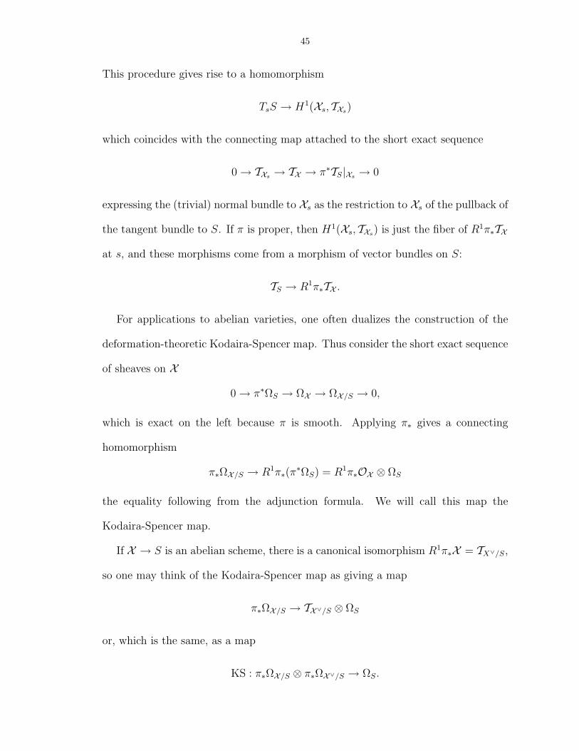
This procedure gives rise to a homomorphism

TsS → H1(Xs, TXs)

which coincides with the connecting map attached to the short exact sequence

0→ TXs → TX → π∗TS|Xs → 0

expressing the (trivial) normal bundle to Xs as the restriction to Xs of the pullback of

the tangent bundle to S. If π is proper, then H1(Xs, TXs) is just the fiber of R1π∗TX

at s, and these morphisms come from a morphism of vector bundles on S:

TS → R1π∗TX .

For applications to abelian varieties, one often dualizes the construction of the

deformation-theoretic Kodaira-Spencer map. Thus consider the short exact sequence

of sheaves on X

0→ π∗ΩS → ΩX → ΩX/S → 0,

which is exact on the left because π is smooth. Applying π∗ gives a connecting

homomorphism

π∗ΩX/S → R1π∗(π∗ΩS) = R1π∗OX ⊗ ΩS

the equality following from the adjunction formula. We will call this map the

Kodaira-Spencer map.

If X → S is an abelian scheme, there is a canonical isomorphism R1π∗X = TX∨/S,

so one may think of the Kodaira-Spencer map as giving a map

π∗ΩX/S → TX∨/S ⊗ ΩS

or, which is the same, as a map

KS : π∗ΩX/S ⊗ π∗ΩX∨/S → ΩS.

46

Remark III.4. The Kodaira-Spencer map is related to the Gauss-Manin connection

∇ as follows: The relative de Rham cohomology bundle H1 := R1π∗(0 → OX →

Ω→ . . .) sits in the Hodge exact sequence

0→ π∗ΩX/S → H1 → R1π∗(OX )→ 0.

The Kodaira-Spencer map is then recovered by composing the maps in this sequence

with ∇; more precisely, it is the map

π∗ΩX/S → H1 ∇→ H1 ⊗ ΩS → R1π∗(OX )⊗ ΩS.

3.4 Katz’s differential operators arising from the Hodge sequence.

The Gauss-Manin connection

∇ : H1 → H1 ⊗ ΩC

on the relative de Rham cohomology bundle on the Shimura curve C is compatible

with the anti-action of EndC(A) on H1 via the rule

∇ φ = (φ⊗ 1) ∇.

(See Proposition 2.2 of [Mo].) The Gauss-Manin connection thus naturally restricts

to a connection on the bundle L1 and extends to the symmetric powers Ln of L1 by

the Leibniz rule

∇(v1 ⊗ v2 ⊗ . . .⊗ vn) =∑i

v1 ⊗ . . .⊗ vi ⊗ . . .⊗ vn ⊗∇(vi).

(When n = 0, the connection is just d : OC → ΩC .)

Using the universal principal polarization on A, we think of the Kodaira-Spencer

map as a map

KS : π∗ΩA/C ⊗ π∗ΩA/C → ΩC .

47

By Theorem 2.5 of [Mo], this map becomes an isomorphism upon restricting to ω⊗ω.

For each j we get a map ∇ : Lj → Lj+2 by composing the maps

Ln ∇ // Ln ⊗ ΩCid⊗KS−1

// Ln ⊗ ω⊗2 // Ln ⊗ L2// Ln+2

where ω⊗2 → L2 is just Sym2 of the inclusion in the Hodge sequence.

Suppose we have a map Ψ : H1 → π∗ΩA/C of vector bundles splitting the Hodge

sequence. (In the cases considered below, the map Ψ will not be an algebraic mor-

phism of vector bundles.) Write Ψr : Ln → ω⊗n for the induced map on Ln.

We then get a “differential operator” Θψ : ω⊗n → ω⊗n+2 by the composition

(3.1) ω⊗n → Lne∇→ Ln+2

Ψr→ ω⊗n+2.

When n = 0, this is just the inverse Kodaira-Spencer map (for any choice of split-

ting). Following Katz, we will apply this formalism in two different settings to attain

differential operators on the spaces of smooth and p-adic modular forms.

3.4.1 The Maass-Shimura operator Θ∞

A real analytic modular form (of weight k and level N+) for B is an analytic

function f(z) satisfying the usual relation

f(γz) = j(γ, z)kf(z)

for γ ∈ ΓB,N+ .

For V a vector bundle on CC, write Vra for the associated real analytic vector

bundle on CC. We will describe a splitting Ψ∞ : H1ra → ωra of real analytic vector

bundles over CC. The Dolbeault complex

OCC → OCC,smooth → Ω0,1CC,smooth → 0

48

is a resolution of OCC ([Vo], Prop. 4.19), so identifies

π∗Ω0,1CC,smooth

∂π∗OCC,smooth

= R1π∗OCC .

Under this identification, the map

H1 → R1π∗OCC

in the Hodge sequence is the natural projection. By Hodge theory, this projection

splits on the level of real analytic bundles, because there is a unique harmonic section

of H1ra in any ∂-equivalence class of relative (0, 1) form. By definition

Ψ∞ : H1ra → ωra

is the induced splitting of the Hodge sequence.

The differential operator coming from the splitting Ψ∞ and the recipe in (3.1)

is written Θ∞ and called a Maass-Shimura operator. It sends real-analytic modular

forms to real-analytic modular forms but does not preserve holomorphy. If we regard

a modular form as a function f on the upper half plane and write the complex variable

z = x+ iy,then ([Mo], Proposition 2.9) the Maass-Shimura operator is given by the

rule

Θ∞(f) =

(d

dz+

k

2iy

)f.

3.4.2 The Ramanujan-Atkin-Serre operator θ

There is a Frobenius morphism φ on the relative de Rham cohomology bundle

H∗(Aord/Cord) over the ordinary locus Cord, semilinear over L, inducing the usual

Frobenius morphism φ on the fibers of this bundle. Moreover, there is a splitting

Ψp of the Hodge sequence (of rigid vector bundles over the ordinary locus), where

R1π∗OAord is identified with the sub-bundle of H|Cord on which φ acts with unit

eigenvalue (see Proposition 2.10 of [Mo]).

49

This splitting Ψp and the recipe in (3.1) give rise to a differential operator θ,

taking p-adic modular forms of weight k to p-adic modular forms of weight k + 2. If

one regards the splitting Ψp as a map of bundles for the p-adic topology on Cord(L),

the same recipe gives rise to an operator on the space of locally analytic modular

forms over the ordinary locus, also written as θ.

3.4.3 Coincidence of the operators at CM points

The following theorem is due to Shimura and Katz.

Theorem III.5. If g is a modular form on C, and P ∈ C(M) is a CM point for

some number field M , then for any choice ω of translation-invariant differential on

A, one has

(θg)(P, ω) = (Θ∞g)(P, ω)

in the sense that both numbers belong to M . (We are using the chosen embeddings of

Q into C and Cp in two ways: first, to get inclusions C(M) ⊂ C(Cp) and C(M) ⊂

C(C), and second, to make sense of the equality.)

Proof. This is shown in many places; see e.g. Theorems 2.4.5 and 2.6.7 of [Ka3] in

more generality or Proposition 2.11 of [Mo] for the Shimura curve case. The point

is that at a CM point, the splitting of H1dR(A′/C) coming from Hodge theory and

the splitting of H1dR(A′/Cp) coming from Frobenius both come from the splitting of

H1dR(A′/M) into the subspace where K acts via the identity and the subspace where

K acts via conjugation, as discussed in Section 2.9.

3.5 Hecke operators and p-adic Hecke operators

Throughout this document, we follow the convention that Hecke operators act on

the right on the space of modular forms, while differential operators act on the left.

50

This convention is unfortunate, as the differential operators and Hecke operators do

not commute. The commutation relation is given by Proposition III.6 below.

For a prime `, a false elliptic curve A over a field k of characteristic prime to ` has

` + 1 cyclic sub-O-modules annihilated by `. Write C0, . . . , C` for these subgroups

and φi : A→ A/Ci for the associated to Ci. If

t : µN+ × µN+

is a V1(N+) level structure on A, and ` - N+, then ti = φi t is a V1(N+) level

structure on A/Ci. If ω is a one-form on A, then there is a unique one-form ωi on

A/Ci with φ∗iωi = ω.

The Hecke operator T` on the space of modular forms of weight k is defined by

the averaging rule

F |T`(A, t, ω) =1

`

∑i=0

F (A/Ci, ti, ωi).

Note that the Hecke operators preserve the weight and level of a modular form, and

also act on the larger space of p-adic modular forms.

Now suppose that A is a false elliptic curve with ordinary reduction over a p-adic

field L. Then there is a unique p-torsion cyclic sub-O-module C of A which reduces

mod p to the kernel of the Frobenius morphism, called the canonical subgroup (this

is Theorem 11.1 of [Kas], although in the case of ordinary reduction one may con-

struct it more simply, following the discussion above the statement of that theorem).

Order the p-torsion cyclic sub-O-modules in such a fashion that C0 is the canonical

subgroup. If F is a p-adic modular form, we get another p-adic modular form F |V

by the rule

F |V (A, t, ω) = F (A/C0,1

pt0, pω0),

51

and a p-adic modular form F |U by the rule

F |U(A, t, ω) =1

p

p∑i=1

F (A/Ci, ti, ωi).

Writing [p] for the operator on the space of modular forms given by

F |[p](A, t, ω) = F (A, pt,1

pω)

one has

Tp = U +1

p[p]V.

One has V U = Id. In particular, the operators UV and V U − UV are idempotent.

Proposition III.6. For any prime ` with (`,N) = 1, including the case ` = p, one

has

(θf)|T` = `θ(f |T`).

Proof. In the modular curve case, this is an easy consequence of the formula for T` on

q-expansions (see paragraph 2.1 of [Se]). We give a proof in Serre-Tate coordinates

in Section 5.5. This proof has the advantage of working for locally analytic modular

forms which are rigid on residue disks (for which there is no q-expansion principle,

even in the classical case).

CHAPTER IV

Serre-Tate coordinates: general theory

This chapter and the next work under a notation scheme which conflicts with the

one introduced in Chapter II. In these chapters (only), we work exclusively over

the ring W of Witt vectors on k = Fp, writing L for its field of fractions. In these

chapters, roman A always refers to abelian varieties over k and cursive A always

to abelian schemes over other W -algebras (in particular, A no longer denotes the

universal false elliptic curve and A no longer denotes the fixed false elliptic curve).

Also, in these chapters, X refers to CL and X refers to its integral model CW .

Fix a residue disk D ⊆ X(L), the space of points reducing to a fixed ordinary

false elliptic curve A/k with level structure t. The ring of rigid analytic functions on

D is obtained from the ring of functions on the formal completion of X at the point

corresponding to A on the special fiber by inverting p. There is a canonical formal

uniformizer for this ring, coming from Serre-Tate theory, which we will use to give

explicit formulas for the operators U , V , and of the preceding chapter. In the next

chapter, we will give those formulas. Before explaining this, we review the basics of

Serre-Tate theory.

52

53

4.1 Serre-Tate coordinates

This section recalls the results of Serre, Tate, and Katz on deformations of ordi-

nary abelian varieties in characteristic p; for a detailed exposition with proofs, see

[Ka2]. Fix a g-dimensional ordinary abelian variety A over k. Write At for the dual

abelian variety. If R is an Artin local ring with residue field k, then a deformation

of A to R is an abelian scheme A over R together with an identification A× k ∼→ A.

Write TpA and TpAt for the “physical” Tate modules of A and At, i.e.

TpA = lim←−A[pn](k).

They are free Zp-modules of rank g (by ordinarity).

Whenever we refer to the Weil pairing on A, we mean the scheme-theoretic Weil

pairing, normalized as in Section 5 of [Ka2] (the classical Weil pairing is trivial in

characteristic p)1). It is a non-degenerate alternating pairing of k group-schemes

epn : A[pn]× At[pn]→ µpn

restricting to a perfect pairing

A[pn]× At[pn](k)→ µpn ,

compatible with the maps p : A[pn]→ A[pn−1]. (Here A is the formal completion of

A at the origin.)

Let A be a deformation of A to R. The formal group A represents the functor

Artin local R− algebras with residue field k → Groups

given by

A(B) = ker(A(B)→ A(k)).1The scheme-theoretic Weil pairing is due to Oda. The standard reference is [KM]; the pairing there is the inverse

of Oda’s pairing and the pairing in [Ka2]. The normalization of the Weil pairing does not affect any of the formulasin this document.

54

Then there is a pairing

qA : TpA× TpAt → Gm(R)

given by the following rule: given Pn ∈ A[pn](k), and Qn ∈ At[pn](k), pick a lift

Pn of Pn to A(R). Consider pnPn ∈ A(R) ⊆ A(R). If n is large enough that

(1 + mR)pn

= 1, then A(R) is killed by pn. Thus it makes sense to compute the Weil

pairing epn(pnPn, Qtn), which is an element of µpn(R), which for n large coincides with

Gm(R). These elements are compatible for large n, which gives the desired map qA.

The Serre-Tate theorem asserts that this construction gives a bijection

Isomorphism classes of deformations of A to R = HomZp(TpA⊗ TpAt, Gm(R)).

In particular, the left hand side, which is a priori only a set, gains the structure of

a Zp-module. Furthermore, this correspondence is functorial in R. More precisely,

writing M for the functor from the category of Artin local rings to the category of

sets given by

M(R) = Isomorphism classes of deformations of A to R,

we have

M = HomZp(TpA⊗ TpAt, Gm).

Because these equivalences are compatible with inverse limits, we may replace the

category of Artin local rings with the category of complete local rings in all of the

preceding discussion (although the recipe for computing the pairing qA only makes

sense over Artin local rings). The following proposition gives us a helpful shortcut

in calculating Serre-Tate coordinates:

Proposition IV.1. If f : A → A′ is a map lifting some map f : A→ A′, P ∈ TpA,

and Qt ∈ TpA′t, then one has

qA(P, f t(Qt)) = qA′(f(P ), Qt).

55

Now, the functorM parameterizing all deformations of our fixed ordinary abelian

variety A is a formal scheme SpfR equipped with a universal formal abelian scheme

π : A → SpfR. Write A for the completion of the universal abelian scheme above

x.

By the above, there is then a bilinear pairing

q bA : TpA⊗ TpAt → 1 + mR,

and by universality, given any deformation A of A over any complete W -algebra R

with residue field k, we have a map R → R making the following triangle commute:

TpA⊗ TpAt

qA???

???

q bA

1 + mR1 + mR //^^^^^

The ring R is the completion of the W -algebra generated by the functions q(P,Qt)−

1, as P and Qt range over TpA and TpAt, respectively, subject to the relations

generated by the bilinearity of the pairing q. In particular, suppose that we pick

bases P1, . . . , Pg and Qt1, . . . , Q

tg of TpA and TpA

t. Then we have g2 elements

qij = q(A, Pi, Qtj) ∈ R, and, writing

Tij = qij − 1

we get a ring isomorphism

R = W [[Tij]].

4.2 Katz’s computation of ∇

Serre-Tate coordinates give us a canonical way to compute the Gauss-Manin con-

nection on the formal relative de Rham cohomology bundle H = R1π∗(Ω·A/R) on

56

residue disks over ordinary points. In this formal setting, there are line bundles

π∗Ω bA/M and R1π∗O bA = Lie(At/R), sitting in the usual Hodge exact sequence

0→ π∗Ω bA/M → H → Lie(At/R)→ 0.

There is likewise a Gauss-Manin connection ∇ : H → H ⊗ ΩSpfR. We will abuse

notation and not distinguish these line bundles from R-modules, starting right now:

Lemma IV.2 (Katz). There are canonical isomorphisms

TpAt ⊗R ∼→ π∗Ω bA/M(?)

and

Hom(TpA,Zp)⊗R∼→ Lie(At/R).,(??)

such that:

• the R-semilinear Frobenius endomorphism Φ of H acts via multiplication by p

on TpAt under the identification (?).

• the sub-Zp-module of H on which Φ acts via the identity maps isomorphically

to Hom(TpA,Zp) under the map H → Lie(At/R) and the identification (??).

Proof. We just recall the construction of the isomorphisms here. For the computa-

tion of the Frobenius action, see Lemma 4.2.1 of [Ka2]. The Weil pairing gives an

isomorphism

TpAt = HomZp(A, Gm),

so given P ∈ TpAt, one gets a differential on A by pulling back dTT

.

Dually (and swapping the roles of A and At), the Weil pairing gives rise to an

isomorphism

At = Hom(TpA, Gm).

57

Applying “Lie” to both sides gives the second result, since for any R one has

ker(

Hom(TpA, Gm(R[ε])→ Hom(TpA, Gm(R)))

=

Hom(TpA, 1 + εR) ≈

Hom(TpA,R).

For Qt ∈ TpAt, write ωQt for the differential form coming from the lemma. If

φ ∈ Hom(TpA,Zp), write ηφ for the image in H of the vector field attached to φ

by the lemma under the Frobenius splitting of the Hodge sequence. Fix a basis

P1, . . . , Pg of TpA, and write P∨i for the dual basis of Hom(TpA,Zp). Then the

Gauss-Manin connection on H is computed as follows:

Theorem IV.3 (Katz). One has

∇ηP∨i = 0

and, for any Qt ∈ TpAt, one has

∇ωQt =∑i

ηP∨i ⊗ dlog q(Pi, Qt).

Proof. This is “version quat.” of the Main Theorem of [Ka2], as is stated in section

4.1 of that paper.

Thus the horizontal sections of the Gauss-Manin connection are generated by

expressions of the form

ωQt −∑i

log q(Pi, Qt)ηP∨i .

The following observation, which is Lemma 3.5.1 of [Ka2], is a simple consequence

of the construction of the isomorphism in Lemma IV.2:

58

Lemma IV.4. Given a map f : A→ B of ordinary abelian varieties in characteristic

p that deforms to a map of universal formal abelian varieties f : A → B, and

P t ∈ TpBt, one has

f∗ωP t = ωf∗(P t).

CHAPTER V

Serre-Tate coordinates: the case of Shimura curves

Recall that this chapter and the previous one use different notation from the rest

of the document; refer to the first paragraph of the previous chapter for a review.

5.1 Serre-Tate coordinates for Shimura curves

Now assume that A is a false elliptic curve over k. In this case, we have a

subfunctorMfalse ofM = SpfR taking an Artin local ring R with residue field k to

the set of “false deformations” of A toR, where a false deformation is a deformationA

of A to R together with an embeddingO → EndR(A) deforming the given embedding

O → Endk(A) (deformations of the extra endomorphisms, if they exist, are unique

– see Theorem 2.4 of [Ka2]).

Proposition V.1. The subfunctor Mfalse of M is a formal subgroup-scheme. The

ring of formal functions Rfalse on Mfalse is the quotient of R by the closed ideal

generated by the relations

q(bP,Qt) = q(P, b†Qt)

for b ∈ O.

Proof. The relations q(bP,Qt) = q(P, b†Qt) are a classical property of the Weil pair-

ing. To see that these are the only relations (which is the remaining content of the

59

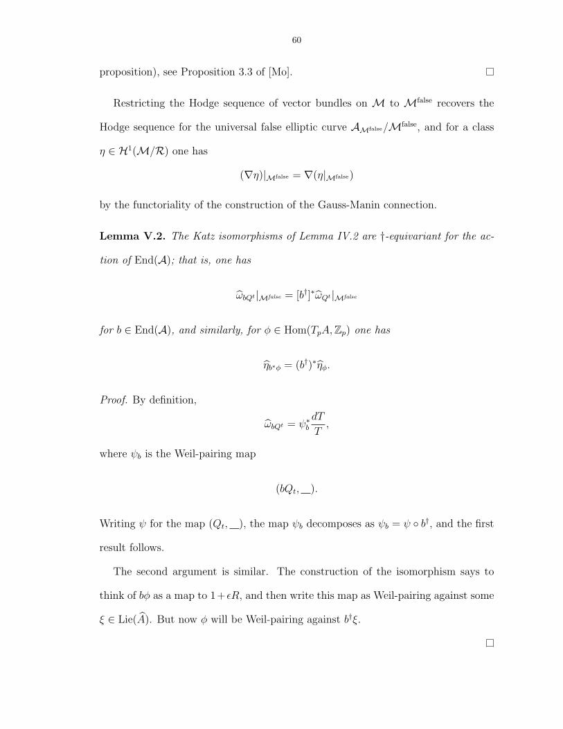
60

proposition), see Proposition 3.3 of [Mo].

Restricting the Hodge sequence of vector bundles on M to Mfalse recovers the

Hodge sequence for the universal false elliptic curve AMfalse/Mfalse, and for a class

η ∈ H1(M/R) one has

(∇η)|Mfalse = ∇(η|Mfalse)

by the functoriality of the construction of the Gauss-Manin connection.

Lemma V.2. The Katz isomorphisms of Lemma IV.2 are †-equivariant for the ac-

tion of End(A); that is, one has

ωbQt |Mfalse = [b†]∗ωQt |Mfalse

for b ∈ End(A), and similarly, for φ ∈ Hom(TpA,Zp) one has

ηb∗φ = (b†)∗ηφ.

Proof. By definition,

ωbQt = ψ∗bdT

T,

where ψb is the Weil-pairing map

(bQt, ).

Writing ψ for the map (Qt, ), the map ψb decomposes as ψb = ψ b†, and the first

result follows.

The second argument is similar. The construction of the isomorphism says to

think of bφ as a map to 1+ εR, and then write this map as Weil-pairing against some

ξ ∈ Lie(A). But now φ will be Weil-pairing against b†ξ.

61

Pick a basis P1, P2 for TpA such that eP1 = P1 and eP2 = 0; denote by P t1, P

t2

the images of P1 and P2 in TpAt under the canonical principal polarization. These

choices give rise to sections of the formal bundles π∗A/X and Lie(At/X ) via the

Katz isomorphisms of Lemma IV.2, which we denote ωP ti and ηP∨i . To compute the

Gauss-Manin connection in the situation that we desire, we will compute it on these

sections over the formal 4-fold M, restrict to Mfalse, then apply e.

Because the Katz isomorphisms in Lemma IV.2 are equivariant for the action of

End(A), one has

e∗

ωP t1 |Mfalse

ωP t2 |Mfalse

ηP∨1 |Mfalse

ηP∨2 |Mfalse

=

ωP t1 |Mfalse

0

ηP∨1 |Mfalse

0

For the remainder of this document, abbreviate e∗ωP1 as ω and e∗ηP1 as η. The

choice of basis of TpA gives us functions q(Pi, Ptj ) for i, j = 1, 2; abbreviate the

particular function q(P1, Pt1) as just q.

Theorem V.3. One has

∇ω = η ⊗ dlog q

∇η = 0.

Proof. This follows from theorem IV.3 and the rule ∇ e = (1⊗ e) ∇.

As a corollary the theorem gives

(5.1) KS(ω⊗2) = dlog q.

5.2 The operator θ in coordinates

Recall that θ is defined by stringing together the maps

62

ωr → Lr∇→ Lr ⊗ Ω

Ψp−→ ωr ⊗ ΩKS−1

−→ ωr+2

To compute the effect of this map on a section ω of the bundle Lr over the ordinary

locus Cord, we compute separately in each residue disk. Thus, along a fixed residue

disk D, write

ω = F (T )ω⊗r

where T = q − 1 is the canonical uniformizer of R coming from Serre-Tate theory,

and F is a power series in T .

Then it follows from Katz’s computation of ∇ and the Leibniz rule that

∇ω =r−1∑i=0

F (T )ω⊗i ⊗ η ⊗ ω⊗r−1−i ⊗ dlog q + F ′(T )ω⊗r

By Lemma IV.2, the splitting Ψp sends η to 0, so

θω = F ′(T )ω⊗r ⊗KS−1(dT ).

Now

dT = q dlog q = (1 + T ) dlog q,

so

θf = (T + 1)F ′(T )ω⊗r+2

by formula (5.1). Thus

θf = (T + 1)d

dTF (T )ω⊗r+2.

This result was originally obtained in the Shimura curve case by Mori ([Mo]).

5.3 Hecke operators in coordinates

We handle T` for ` 6= p first. Suppose ψ : A→ A/C is an isogeny of degree prime

to p. Then the subgroup C and the map ψ deform uniquely to a subgroup scheme

63

C and a map ψ : A → A/C for any lift A of A to L. Recall the fixed generator

P1 of eTpA. Because ψ and ψt both induce isomorphisms of p-adic Tate modules,

Qt1 := (ψt)−1(P t

1) is a generator of eT tp(A/C). Write ω1 := eωP t1 for the canonical

formal one-form on the disk D ⊂ X(L) whose points correspond to characteristic

0 abelian surfaces reducing to A/C with level structure ψ(t). By Lemma IV.4, It

satisfies

ψ∗ω1 = ω.

Given this choice of Qt1, there is a corresponding basis element of Tp(A/C) via

the canonical principal polarization of A/C, which is Q1 = 1degψ

ψt(Qt1). Thus there

is a Serre-Tate coordinate q = q( , Q1, Qt1) on the disk D.

Lemma V.4. The function fψ on D given by A 7→ q(A/C) can be computed as

fψ = q1

degψ

Proof. It suffices to check that the two functions agree for any deformation A of A

to an Artin local ring R with residue field k. It follows from Proposition IV.1 that

fψ(A) = q(A/C, Q1, Qt1)

= q(A/C, 1

degψψt(P1), Qt

1)

= q(A, 1

degψP1, P

t1)

= q(A)1

degψ

Note that the final expression does not depend on any choices, as the Serre-Tate

parameter q is a principal unit and degψ is prime to p.

64

Corollary V.5. For each cyclic degree ` isogeny A → A/Ci of A, write ωi for the

canonical one-form on the disk Ri of points reducing to A/Ci, as normalized above.

Suppose f is a modular form such that for each i, the Serre-Tate expansion on the

disk Di is

f = Fi(Ti)ω⊗ki

Then on the disk D, f |T` is given by

`+1∑i=1

Fi((1 + T )1/` − 1)ω⊗k.

We move on to the operators U and V . Write φ for the mod p Frobenius. For D

an ordinary residue disk corresponding to a false elliptic curve A with level structure

t, write Dφ for the disk corresponding to Afrob with level structure 1ptφ. Note that,

because of the extra factor of 1p

on the level structure, Dφ is not the image of D

under the map Xord → Xord under the canonical p-isogeny A → A/C0.

We are going to pick Serre-Tate coordinates on these disks in a compatible way.

One cannot ensure, as in the prime-to-p case, that the canonical formal one-form

pulls back to the canonical formal one-form. However, using ordinarity, we do at

least have that Q1 := φP1 is a basis for eTpAφ. Write Qt

1, Qt2 for the corresponding

basis for TpAφ,t, using the principal polarization on A. Then one has

φt(Qti) = pP t

i

Write q1 for the function on Dφ corresponding to this basis. There is a function f

on D = D0 given by (A, t) 7→ q1(A/CA, 1ptφ), where CA is the canonical subgroup of

A.

Lemma V.6. One has

f = qp

65

as functions on D.

Proof. Again it suffices to check that the two functions agree for any deformation A

of A to an Artin local ring R with residue field k. One has

f(A) = q(A/C, φP1, Qt1)

= q(A, P1, φtQt

1)

= q(A, P1, pPt1)

= q(A)p

Let ω0 be the canonical formal relative one-form for D0 attached to the Tate-

module generators φP1, φP2. Write Φ : D → D0 for the “quotient by the canonical

subgroup” map.

Lemma V.7. One has

Φ∗ω0 = pω

Proof. This follows from Lemma IV.4.

Corollary V.8. If f =∑F (T )ω⊗k0 is a modular form on Dφ expressed in Serre-

Tate coordinates, then the corresponding modular form f |V is given in Serre-Tate

coordinates on D by

f |V = F ((1 + T )p − 1)ω⊗k

Finally, we compute U . For 1 ≤ i ≤ p, write Di for the image of D under the

map Xord → Xord under the (not-canonical) p-isogenies A → A/Ci. Then the map

D → Di → (Di)φ is the identity map (because of the factor of 1/p in the level

structure). For each subgroup C other than the canonical subgroup of the universal

66

false elliptic curve over D, there is a function gC given by (A, t) 7→ qi(A/C, Imaget),

where C = CA.

Lemma V.9. One has

gpC = q

Proof. This follows from Lemma V.6, because (A/C)t → At is the canonical isogeny

for (A/C)t.

Fix a primitive pth root of unity ζ ∈ Cp.

Lemma V.10. There is an ordering on the disks Di such that on Ci one has

gCi = ζ iq.

Proof. It follows from the preceding lemma that there is some root of unity making

the lemma true; the content of the lemma is that each distinct root of unity appears

exactly once. To figure out which root of unity shows up on the disk Di, we may

evaluate at qi = 1, i.e. at the CM point on the disk Di. This calculation is done by

Brakocevic in the GL2 case, using Shimura’s reciprocity law for GL2 (see the proof

of Lemma 7.2 of [Br]).

To reduce to the GL2 case, note that, by the argument on p. 918 of [Pr], there is

a false isogeny (defined over a number field in which p is unramified)

λ : A → E1 × E2

of A with a product of elliptic curves, with degree prime to p. The result then follows

from Proposition IV.1.

The pth roots of q in the ring of Cp-valued functions on D are given by Taylor-

expanding ζ i(1+T )1/p. Write Φi : D → Di for the map killing the ith (non-canonical)

subgroup.

67

Lemma V.11. One has Φ∗ωi = ω

Proof. This follows from Lemma V.7, since the degree of Φi is p.

Proposition V.12. If f =∑Fi(T )ω⊗k is a rigid-analytic modular form on Di

expressed in Serre-Tate coordinates, then the corresponding modular form f |U is

given in Serre-Tate coordinates on D by

f |U(T ) =1

p

p−1∑i=0

F (ζ i(1 + T )1/p − 1)ω⊗k.

Proof. Just a restatement of the preceding two lemmas. Note that it makes sense

to evaluate F at (ζ i(1 + T )1/p − 1), as the constant coefficient of ζ i(1 + T )1/p − 1 is

ζ i − 1, which lives in the maximal ideal of W [ζ].

The importance of the above formulas is that they give a formula for the compo-

sition UV of Hecke operators (the composition V U is the identity).

Proposition V.13. Suppose that f has Serre-Tate expansion

f = F (T )ω⊗k

on the disk D. Then f |UV has Serre-Tate expansion

f |UV (T ) =1

p

p−1∑i=0

F (ζ i(1 + T )− 1)ω⊗k.

Moreover, if F (T ) ∈ W [[T ]], then 1p

∑p−1i=0 F (ζ i(1 + T )− 1) ∈ W [[T ]].

Proof. Write f = Fφ(T )ω⊗k in Serre-Tate coordinates on the disk Dφ.

We compute

(F (T )ω⊗k)|UV = (Fφ((1 + T )p − 1)ω⊗k0 )|U

=1

p

p−1∑i=0

F (ζ i(1 + (1 + T )p − 1)1/p − 1)ω⊗k

= F (ζ i(1 + T )− 1)ω⊗k.

68

The integrality claim for this expression is well-known (see e.g. p. 16 of [CS]). To

prove it, note thatp−1∑i=0

F (ζ i(1 + T )− 1)

has coefficients in the maximal ideal p of W [ζ], because it reduces to 0 mod (1− ζ).

Thus the coefficients lie in p ∩W = (p).

5.4 Continuity properties of the operators

Write Θ for the operator (1 + T ) ddT

on the ring W [[T ]], so what we have seen so

far is that

θ(F (T )ω⊗k) = (ΘF )(T )ω⊗k+2.

In this section, we investigate elementary continuity properties of the operator Θ use

them to deduce similar properties for θ on the space of p-adic modular forms.

Proposition V.14. The Θ operator satisfies the continuity condition

ΘiF ≡ ΘjF mod pn

for any F and any i, j ≥ k such that i ≡ j mod (p− 1)pn−1.

Proof. First suppose that F is a polynomial. Setting x = 1 + T , on the ring W [x] =

W [T ] ⊆ W [[T ]], we have Θ = x ddx

, so θi∑anx

n =∑nianx

n and the result follows

(using Fermat’s little theorem for the terms with (p, n) = 1 and the condition i, j ≥ k

for the others).

To establish the result for a general power series F =∑bnT

n, we may fix n and

prove that the congruence holds for the coefficients of T n in ΘiF and ΘjF . Note

that the coefficient of T n in ΘF depends only on the coefficients of T n and T n+1 in

F . Thus, the coefficient of T n in ΘiF depends only on the numbers bn, bn+1, . . . , bn+i,

and similarly for ΘjF . It follows that there exists a polynomial truncation G of F

69

such that the coefficients of T n in ΘiG and ΘjG are the same as those for F . Since

the congruence holds for polynomials, the result follows.

Corollary V.15. Suppose that f is a p-integral modular form, i.e., that f is a

modular form over some subring of W . Then for any ordinary pair (A, ω) one has

θif(A, ω) ≡ θjf(A, ω) mod pn

whenever i ≡ j mod (p− 1)pn−1.

Write f [ = f |V U−UV , and similarly for F ∈ W [[T ]] we write F [ = F |VU−UV,

where UV is the formal operator on power series of Theorem V.13 and VU is the

identity operator.

Proposition V.16. One has

F [ = limi→∞

Θpi(p−1)F.

Proof. The limit on the right hand side makes sense because of Proposition V.14.

Writing Θ(p−1)p∞ for the operator limi→∞Θpi(p−1), we see that Θ(p−1)p∞ is a contin-

uous W -linear operator on W [[T ]]. As this is also the case for the operator [, it

suffices to check the putative equality on the polynomials Fm = (1 + T )m, since the

linear span of these polynomials is dense. One has ΘiFm = miFm, and so

Θ(p−1)p∞Fm =

0, p|m

Fm, (p,m) = 1.

On the other hand, using Proposition V.13, we compute

F [m(T ) = Fm(T )− 1

p

p−1∑i=0

Fm(ζ i(1 + T )− 1)

= Fm(T )− 1

p

p−1∑i=0

ζmi(1 + T )m.

70

If p is prime to m, then the sum is zero, since ζmi ranges over a complete set of

pth roots of unity. If p divides m, the sum is Fm(T ). In either case F [m = Θ(p−1)p∞Fm

as desired.

We return to the operators θ, U , and V on the space of p-adic modular forms. If f

is a p-adic modular form, and (A′, t′, ω′) is a triple consisting of a false elliptic curve

over L with ordinary reduction, level structure, and a translation-invariant one-form,

then the limit

limi→∞

θpi(p−1)f(A′, t′, ω′)

exists and equals f [(A′, t′), since this statement can be checked on residue disks. In

particular, if j is a negative integer, it makes sense to write

θjf(A′, t′, ω′)

to mean

limi→∞

θj+pi(p−1)f.

A priori, θjf is a locally analytic modular form, rigid when restricted to a fixed

residue disk. Note that, in spite of the notation, one has θkθ−kf = f [, not f .

5.5 Proof of Proposition III.6

We conclude by proving the formula

(θf)|T` = `θ(f |T`)

as promised. In each case the result follows from the explicit formulas for the Hecke

operators (using the chain rule). For ` 6= p, this is a simple calculation. For Tp it

will follow from related formulas for U and V , using the formula

Tp = U +1

p[p]V.

71

Letting ψ denote the automorphism of X mapping (A, t) to (A, pt), it follows directly

from the modularity of f that

f |[p] = pkf ψ,

and thus

θ(f |[p]) = p−2(θf)|[p]

(because θ boosts the weight of f by 2). The chain rule argument gives that

θ(f |V ) = p(θf)|V

and

pθ(f |U) = (θf)|U ,

which is the desired result.

CHAPTER VI

Twisted cohomology groups and residue theory

6.1 Review of Deligne’s twisted cohomology groups

Let X/C be a variety, and suppose that V is a local system on X(C), that is, a

sheaf locally (for the complex topology) isomorphic to the constant sheaf Cg. Deligne

[De] then showed how to recover the cohomology groups H i(X(C),V) algebraically,

generalizing the case V = C of algebraic de Rham cohomology. Recall that the vector

bundle V = V ⊗C OX is algebraic, as is the connection V → V ⊗ Ω for which V is

the sheaf of horizontal sections (see Section 3.2.1). Then H i(X(C),V) coincides with

the hypercohomology of the complex

(6.1) 0∇→ V ⊗ Ω

∇→ V ⊗ ∧2Ω∇→ . . .

Write H idR(X,V ,∇) for the ith hypercohomology group of this complex. Of course

these algebraic definitions all make sense over an arbitrary base field k (they are not

useful unless the characteristic of k is zero).

Given two vector bundles V ,V ′ with flat connections ∇,∇′, the natural map of

the complexes (6.1) for V ,V ′, and V ⊗ V ′ gives rise to maps

H i(X,V ,∇)⊗Hj(X,V ′,∇′)→ H i+j(X,V ,∇⊗∇′).

We will apply this observation in particular to the case where (V ,∇) is self-dual, so

that the target is the ordinary algebraic de Rham cohomology of X.

72

73

As in the case where V is the trivial local system, we get a “Hodge sequence”

0→ H0(X,V ⊗ Ω)→ H1(X,V ,∇)→ H1(X,V),

as can easily be seen by taking a Cech resolution of (6.1).

The remaining sections of this chapter are used only in the proof of Proposition

VIII.1, which is extremely similar to the proof of Proposition 3.18 of [BDP]. The

reader who is already familiar with the arguments in [BDP], or who wishes to take

the statement of Proposition VIII.1 on faith, may prefer to skip to the next chapter.

6.2 Residues, algebraically

If X is a smooth curve over a field k, Tate gave an algebraic definition of the

residue of a meromorphic one-form at a point. Residue theory gives us a canonical

way to compute the algebraic de Rham cohomology of X. As is well-known, these

results carry over to meromorphic forms valued in vector bundles on X with flat

connections.

Throughout this section, V is a vector bundle on X with a connection ∇ which

is integrable (flat). For P a point of X, write V(P ) for the fiber of V above P .

Definition VI.1. If U ⊆ X is open, then ∇ trivializes on U if V(U) admits a basis

of horizontal sections for ∇.

Remark VI.2. The condition that ∇ trivializes on U is stronger than the condition

that V trivializes on U . For example, a connection on the trivial bundle O is none

other than a one-form ω, and the connection corresponding to ω trivializes on an

open set U if and only if there is a function f on U solving the differential equation

(6.2) dlogf = ω.

74

If a connection admits a trivialization on an open set U , we may define the residue

of a meromorphic section at a point P ∈ U by stringing together the maps

(6.3) V ⊗ Ω⊗K(U)f→ Ωn(U)

resP−→ kn = (On)(U)d=0 f−1

−→ V(U)∇=0 = V(P ),

where resP denotes the Tate residue map (formally expand in a parameter t at P

and take the coefficient of t−1).

The residue does not depend on the choice of trivialization because any choice

differs by an element of GLn(C), for which the classical residue map is linear (note

that if we insisted only on trivializing the vector bundle and not the connection, the

ambiguity would be up to GLn(O), and the residue would depend on the choice).

As shown already, the Gauss-Manin connection admits local trivializations in the

rigid topology, but not in the Zariski topology. However, in characteristic zero, any

integrable connection admits a trivialization in a formal neighborhood of a point:

that is, writing OP for the completion of the local ring at P and VP for the completion

of the stalk of V at P , there exists a trivialization f making the following square

commute:

(6.4)

VPf //

∇

OnPd

V ⊗ ΩP

f // ΩnP

To see this, pick a trivialization of V in a formal neighborhood of a point, and then

write down a formal solution to Equation 6.2. Since this trivialization always exists,

we use it, rather than (6.3) in the definition below of residues for arbitrary vector

bundles with flat connection; in practice, the residues in this document are computed

in the rigid topology.

Definition VI.3. The residue of a meromorphic section of V ⊗ Ω with connection

75

∇ at a point P is the element of the fiber of V at P given by the maps

V ⊗ Ω⊗KPf→ Ωn

P

resP−→ kn = (OnP )d=0 f−1

−→ VP∇=0

= V(P )

where f is a choice of trivialization.

Proposition VI.4. The twisted first algebraic de Rham cohomology

H1(X,V ,∇)

can be computed as the space of ∇-closed V-valued one-forms with residue zero at

every pole modulo ∇-exact forms.

Proof. This is a direct generalization of Tate’s technique for computing the algebraic

de Rham cohomology of curves, which is the case V = O and ∇ = d. Write K for

the function field of X, thought of as a constant sheaf on X. Then the complex

0→ V ∇→ V ⊗ Ω→ 0

has a resolution coming from the double complex

V

// V ⊗ Ω

V ⊗K

// V ⊗ ΩK/k

⊕P∈U

(V ⊗K)PVP

//⊕VP ⊗ ΩKP

OP

where all horizontal arrows are induced by ∇. The condition that a meromorphic

V-valued form have residue zero at every pole is exactly the condition that it have

∇-primitives in the completion of V at every point. Such primitives are well defined

up to ∇-horizontal, in particular holomorphic, sections, so the result follows as in

the classical case.

76

Finally, suppose that V is self-dual. Then we get a cup product pairing on hyper-

cohomology:

H1(X,V ,∇)⊗H1(X,V ,∇)→ H2dR(X) = k,

which can be computed by the rule

(λ, µ) =∑

resP 〈LP , µP 〉.

where LP denotes a ∇-primitive for λP , defined in some neighborhood of P , and the

quantity on the right is the residue of an honest meromorphic one-form.

6.3 Coleman’s rigid analytic theory of residues

Let X/Cp be a curve with good reduction and V a vector bundle on X with

flat connection. Write Xrig for the associated rigid analytic space and Vrig for the

analytification of V .

For any point P ∈ X(Cp), write DP for the residue disk containing P , which

is isomorphic as a rigid space to the open unit disk. Fixing one such isomorphism

taking P to 0 allows us to speak of the affinoid subdomain of DP given by “the

closed disk of radius r” for any r < 1, denoted DP,r. Fixing a finite number of points

P1, . . . , Pn, consider the affinoid space

A = Xrig \DP1 \ . . . \DPn

and its “basic wide-open neighborhoods” (for various choices of radii ri with 0 <

ri < 1)

Wr1,...,rn = Xrig \DP1,r1 \ . . . \DPn,rn .

For ω a one-form on an annulus, Coleman has defined a notion of “residue” which

coincides with the algebraic notion of residue when ω comes from an algebraic one-

form. Using this definition, together with the formalism of the previous section, it

77

similarly makes sense to speak of residues of vector-bundle-valued one-forms on an-

nuli, provided that the vector bundle comes with a flat connection that trivializes on

sufficiently small disks. Coleman’s residue is only well-defined up to a sign (depend-

ing on the “orientation” of the annulus), but he shows in Corollary 3.7a of [Co2] that

one can compatibly orient all the annuli DPi \DPi,ri by choosing a uniformizer of the

deleted point as a uniformizer in the ring of rigid functions on the annulus (instead

of choosing the reciprocal of a uniformizer). Here “compatibility” implies that the

residue of a meromorphic one-form on a Zariski open will agree with the residue of

the same form thought of as a rigid one-form on an annulus, rather than with its

negative.

Coleman has shown that the algebraic de Rham cohomology of the affine curve

X \P1, . . . , Pn can be computed analytically as the “honest” de Rham cohomology

of any wide open neighborhood of A:

Theorem VI.5 (Coleman). For any wide open neighborhood W, the natural map

H1dR(X \ P1, . . . , Pn,V ,∇)→ VW ⊗ ΩW

∇VW

is an isomorphism.

Write H1dR(W ,V ,∇) for

VW ⊗ ΩW∇VW

.

The following two immediate consequences of Coleman’s theory are immediate:

Corollary VI.6. Any inclusion of wide-opens A ⊂ W ⊂ W ′ induces an isomorphism

H1dR(W ′,V ,∇)

∼→ H1dR(W ,V ,∇).

Corollary VI.7. The image of the natural map

H1dR(X,V ,∇)→ VW ⊗ ΩW

∇VW

78

is the space of classes of rigid 1-forms on W with residue zero at each of the points

Pi.

If V is a vector bundle with flat connection, then a primitive for a V-valued

one-form ω (over some open set) is a section Fω of V with ∇Fω = ω. Of course, a

primitive is only unique up to horizontal sections of V . In the p-adic setting, Coleman

has shown a canonical way to write down a primitive for sections of V in the event

that V is equipped with some extra structure coming from the Frobenius map on the

reduction of X. For more details on the following, the reader should consult Section

10 of [Co].1

The reduction X0p of A is a smooth affine curve which admits the p-power abso-

lute Frobenius map to itself. If the set P1, . . . , Pn is Frobenius stable (which one

may always assume by adding more points to it), then, using the good reduction

hypotheses, Coleman shows this Frobenius map lifts to a semilinear map φ : A → A.

Fix a choice of such a φ once and for all.

Definition VI.8. A Frobenius neighborhood of A in W is a pair (W ′, φ), where W ′

is a basic wide open neighborhood with A ⊂ W ′ ⊂ W and φ :W ′ →W restricts to

φ on A.

Definition VI.9. An overconvergent Frobenius isocrystal on an affinoid A is a pair

(V ,Fr) where V is a vector bundle with flat connection ∇ on W and Fr is a ∇-

horizontal morphism

Fr : φ∗V|W ′ → V|W ′

on some Frobenius neighborhood W ′ of A in W .

1In that section, Coleman uses the phrase “over-convergent F -crystal” to mean what this document and otherscall an “overconvergent Frobenius isocrystal.” Moreover, Coleman does not limit his theory to the good-reductioncase, which requires him to distinguish between the “flab”-sheaf of locally analytic sections of V and a certain “flog”sub-sheaf.

79

Given an overconvergent Frobenius isocrystal V , there is an endomorphism Φ of

the space

H1dR(W ,V ,∇)

given by the composition

H1dR(W ,V ,∇)→ H1

dR(W ′, φ∗V ,∇)→ H1dR(W ′,V ,∇) = H1

dR(W ,V ,∇).

Definition VI.10. A polynomial P (T ) ∈ F [T ] is a Coleman polynomial for a class

[ω] ∈ H1(W ,V ,∇) if the following hold:

• P (Φ∗)([ω]) = 0.

• P (Φ) induces an automorphism of the space of locally analytic sections of V

that are horizontal for ∇.

• P (1) 6= 0.

Theorem VI.11 (Coleman). Suppose that ω is a V-valued one-form onW such that

the cohomology class [ω] ∈ H1(W ,V ,∇) admits a Coleman polynomial P (T ). Then

there is a unique locally analytic primitive Fω for ω such that P (Φ∗)Fω is a rigid

section of V on some Frobenius neighborhood of A in W. Moreover, Fω is rigid on

any fixed residue disk of A.

The function Fω is called the Coleman primitive for ω. It turns out that it depends

on none of the choices involved in stating Theorem VI.11 – that is, it does not

depend on W ′, the extension of φ to W ′, nor on the Coleman polynomial (provided

that a polynomial exists). Of course, we will apply this theory in the setting of

L2r on the ordinary locus of C (and its trivial enlargement L2r,2r). In this case,

the overconvergent Frobenius isocrystal structure comes from an extension of the

canonical morphism Aord → Aord to a wide open neighborhood W of the ordinary

80

locus, as is constructed in Chapter 11 of [Kas]. It follows as on p. 42 of [Co] that

there is a Coleman polynomial for the L2r-valued differential form which is the class

of any newform of weight 2r + 2.

The following lemma will be useful in the proof of Proposition VIII.1.

Lemma VI.12. Given an overconvergent Frobenius isocrystal (V ,Fr) on an affinoid

A, a pairing on V that is compatible with the connection, [ω] ∈ H1(W ,V ,∇) a

cohomology class on a wide open neighborhood of A admitting a Coleman primitive

Fω, and [ηfrob] ∈ H1(W ,V ,∇) a cohomology class that is fixed by Frobenius, one has

n∑i=1

resPi〈Fω, ηfrob〉 = 0.

Proof. This is Lemma 3.20 of [BDP].

CHAPTER VII

Construction of the cycle

7.1 Projectors on Kuga-Sato varieties and the cohomology of Shimuracurves

Recall that C is the Shimura curve over F , f is a modular form of weight k = 2r+2

on C, Ar is the r-fold fiber product of the universal false elliptic curve over C with

itself, A is a fixed “CM false elliptic curve,” and Wr = Ar × Ar. In this chapter

we construct a homologically trivial cycle on Wr, then begin our discussion of the

p-adic Abel-Jacobi map, as applied to this cycle. For the first two sections we assume

r > 0. The case r = 0 (so Wr = C) is treated separately in a section at the end of

this chapter.

As in [BDP], our cycle will be the graph of a morphism of false elliptic curves,

modified by an idempotent in the ring of correspondences on a Kuga-Sato variety.

All rings of correspondences in this chapter are taken with rational coefficients.

Recall the bundle L2r = Sym2r eH1.

Theorem VII.1 (Besser). There is a projector P in the ring

CorrC(Ar)

of algebraic correspondences on Ar fibered over C, with the property

PH∗(Ar/C) = PH2r(Ar/C) = L2r.

81

82

Proof. For completeness, we outline Besser’s construction here. The construction is

a bit lengthy, and is broken into a series of small propositions. None of the properties

of P except the one quoted in the statement of the theorem will be used in the sequel.

Therefore, the reader approaching the subject for the first time may wish to grant

the statement of this theorem and skip to Lemma VII.4. Besser makes the projector

in the following steps:

1. There is a projector Q in the ring of C-correspondences on A with QH2(A/C) =

Sym2 eH1(A/C).

2. There is a Kunneth projector P1 in the ring of C-correspondences on Ar with

P1H∗(Ar/C) = SymrQH2(A/C).

3. There is a projector P2 in the ring of C-correspondences onAr with P2 SymrQH2 =

Sym2r eH1(A/C) (under the identification from Step 1).

For step one, a calculation (which may be performed fiber for fiber and thus after

choosing a trivialization of B ⊗K and a basis) identifies Sym2 eH1(A/C) with the

common kernel of the operators b−N(b) acting on H2(A/C).

The existence of the Kunneth projector (step two) is a famous theorem of Deninger

and Murre, which holds for an arbitrary abelian scheme (more precisely, one uses

the work of Deninger and Murre to project to ⊗rQH1, then applies a standard

symmetrizing projector).

In explaining step three, we will not follow the notation of the document at large.

Fix a field L of characteristic zero and let V be a two-dimensional vector space over

L. By convention, Symk V denotes the subspace of⊗k V fixed by the action of Sk.

Let r be a positive integer. There is a natural inclusion

Sym2r V → Symr Sym2 V

83

where⊗r⊗2 V is identified with

⊗2r V without reordering factors.

Now fix a non-degenerate alternating form 〈 , 〉 on V . This gives a map⊗r⊗2 V →⊗r−2⊗2 V by the rule

(v11 ⊗ v12)⊗ . . .⊗ (vr1 ⊗ vr2) 7→∑i<j

〈vi1, vj1〉〈vi2, vj2〉(

(v11 ⊗ v12)⊗ . . .⊗ (vi1 ⊗ vj1)⊗ . . .⊗ (vi2 ⊗ vj2)⊗ . . .⊗ (vr1 ⊗ vr2)).

The restriction of this map to Symr Sym2 V lands in Symr−2 Sym2 V ; call this

restricted map ∆.

Proposition VII.2. The natural inclusion Sym2r V → Symr Sym2 V identifies Sym2r V

with the kernel of ∆.

Proof. By dimension-counting, it suffices to show that Sym2r is in the kernel of ∆

and ∆ is surjective. For the former claim, write

w =1

(2r!)

∑σ∈S2r

σw

and note that, for fixed i < j, the contribution from σw to ∆w cancels the con-

tribution from στw, where τ is the transposition interchanging the positions i1 and

j1.

For the surjectivity, write W for Sym2 V . The form 〈 , 〉 induces a symmetric

form on W ; we may assume L = C and pick an orthonormal basis x, y, z for W .

With respect to this basis, the operator ∆ is just (a scalar multiple of) the usual

Laplace operator∑

∂2

∂x2i, for which the result is well-known.

Now suppose that V and W are finite dimensional vector spaces equipped with

non-degenerate bilinear forms 〈 , 〉. If T : V → W is surjective, then

Ker(T ∗T ) = KerT

84

and

Im(T ∗T ) = (KerT )⊥.

(The first claim is clear, and anything of the form T ∗Tv is certainly orthogonal to

the kernel of T . The second claim then follows by dimension counting.)

Lemma VII.3. Let f : V → V be an endomorphism. Suppose f |Im f is injective,

and write P for the characteristic polynomial of f |Im f . Then

− P (f)

det f |Im f

is a projector onto the kernel of f .

Proof. The Cayley-Hamilton theorem implies that P (f) maps V to ker f , and −P (f)det f

is the identity on ker f because P (f)|ker f = P (0) = − det f |ker f .

In particular, let P be the characteristic polynomial of ∆∗∆|(Ker ∆)⊥ . Then P (∆∗∆)

is a projector onto Sym2r V .

By the preceding (applied fiber-for-fiber), Step Three of Besser’s construction

then follows from the fact that ∆ : H2r(Ar/C) → H2r(Ar−2/C) is induced by a

C-morphism Ar−2 → Ar. To see this last fact, consider the morphisms

φij : Ar−2 ×C A → Ar

given in coordinates by

(a1, . . . , ar−2)× a 7→ (a1, . . . , ai−1, ai, ai, . . . , aj−1, a, aj, . . .)

Then

∆ =∑i,j

φ∗ij

85

Lemma VII.4. For any r > 0,

H0(C,L2r,∇) = 0.

Proof. This can be computed this after base changing to C, and thus (thanks to

GAGA for differential operators as in [De]) it suffices to show it for the local system

Sym2r eR1π∗Q

on the Riemann surface C(C). This local system corresponds to the representation

Sym2r e(C4) of π1(CC) = Γ for which there are no fixed points.

Corollary VII.5. The projector P satisfies

PH∗dR(A) = H1(C,L2r,∇)

Proof. We first show

PH2r+1dR (A) =

⊕p+q=2r+1

Hp(C,PHq,∇) = H1(C,L2r,∇).

The first equality, known (without the P ) as Lieberman’s trick, is true for any abelian

scheme X → S. Lieberman’s observation is that the Leray spectral sequence

Ep,q2 = Hp(S,Hq(X/S),∇)⇒ Hp+q

dR (X)

degenerates at page 2, as the multiplication maps [m] : X → X must on the one

hand commute with the edge maps but on the other induce multiplication by mq on

Ep,q2 . This identifies Hp(S,Hq(X/S),∇) with the mq eigenspace of [m] on Hp+q

dR (X).

The second equality follows from Proposition VII.1.

To see that

PH∗dR(A) ⊂ H2r+1dR (A),

observe that P annihilates HpdR(C,Hq,∇) unless p = 0, 1 and q = 2r. As r > 0 the

latter bundle has no global sections by Lemma VII.4.

86

There is a natural inclusion

H0(X,ω⊗r ⊗ ΩC)→ H1dR(C,L2r,∇)

coming from the hypercohomology spectral sequence. This inclusion identifies the

former vector space with Fil1 = Fil2 = . . . = Fil2r of the latter.

Proposition VII.6. There is a projector εA ∈ Corr2r(Ar, Ar) such that

εAH∗dR(Ar) = Sym2r eH1

dR(A)

Proof. Take the image of Besser’s projector P under the “evaluation at τ” map

CorrC(Wr)→ CorrF (Ar)

Consider the variety Wr together with the projector ε = PεAr in CorrrX(Wr,Wr).

Recall the local system L2r,2r on C which is L2r ⊗ Sym2r eH1dR(A); the fiber of L2r,2r

at a point P of C(F ) corresponding to a false elliptic curve A′ is Sym2r eH1(A′) ⊗

Sym2r eH1dR(A).

Proposition VII.7. One has

εH∗dR(Wr) = H1(C,L2r,∇)⊗ Sym2r eH1dR(A) ⊆ H2r+1(Ar)⊗H2r(Ar) ⊆ H4r+1(Wr).

Proof. This follows immediately from the Kunneth formula.

7.2 The generalized Heegner cycle and the p-adic Abel-Jacobi map

For any N+-torsion point PA on A and any false isogeny φ : A→ A′ whose kernel

intersects the subgroup generated by PA trivially, there is a point PA′,(φ(PA) on C,

87

and an embedding of the graph Γφ into the fiber A × A′ of W1 above this point.

Write Υφ for the rth power of Γφ. The cycles studied in this paper are given by

∆φ = εΥφ.

Note that Υφ has codimension 2r+1 in Wr. It follows that the cycle class map takes

Υφ to H4r+2dR (Wr), and so ∆φ is cohomologically trivial by Proposition VII.7.

7.2.1 The p-adic Abel-Jacobi map

Write Fp for the completion of F at the place above p induced by the chosen

embedding Q → Cp. Recall that for a variety X, CHi0(X) denotes the group of

homologically trivial cycles of codimension i, modulo rational equivalence.

There is a sequence for etale cohomology with supports: for a closed immersion

Z → X of schemes with complement U , then for any sheaf F one has

. . .→ H iZ(X,F)→ H i(X,F)→ H i(U,F)→ H i+1

Z (X,F)→ . . .

If Z and X are smooth over an algebraically closed field and F is a locally constant

`n-torsion sheaf, then there are also (functorial) Gysin maps computing the relative

cohomology groups in terms of the ordinary cohomology groups of Z; writing c for

the codimension of Z in X, the Gysin map identifies

Hj−2c(Z,F(−c)) = HjZ(X,F).

To apply these general facts, write WP for the fiber of Wr above P (which has

codimension 1) and W [ for its complement. By construction, the cycle ∆φ is sup-

ported on WP . Choose i = 4r+ 1 and F = Zp((2r+ 1)). After base changing to the

algebraic closure and applying ε to the Gysin sequence, we get an exact sequence of

88

Galois modules

(7.1)

0→ εH4r+1(Wr,Qp((2r+1)))→ εH4r+1(W [,Qp((2r+1))→ εH4r(WP ,Qp((2r+1)−1)→ 0

using Proposition VII.7 for exactness at the left and right.

There is a map Qp → εH4r(WP ,Qp((2r+1)−1) sending 1 to the class of ∆φ. Define

ξ ∈ Ext1Galois modules(Qp, εH

4r+1(Wr,Qp((2r+ 1))) = H1(Fp, εH4r+1(Wr,Qp((2r+ 1)))

by pushing out the sequence (7.1) along this map.

Write V for the Galois representation εH4r+1(Wr,Qp((2r + 1)). It follows from

work of Nekovar ([Ne1]) that this class ξ lies in the subgroupH1f (K, εH4r+1(Wr,Qp((2r+

1))) defined in [BK], i.e. that the corresponding extension of Galois modules is crys-

talline. The subgroup H1f is the image of the Bloch-Kato exponential map, which is

the connecting map in the long exact sequence in cohomology coming from the short

exact sequence of Galois modules

0→ W → Bφ=1cris ⊗ V ⊕ Fil0BdR ⊗ V → BdR ⊗ V → 0.

Because Dcris(V )φ=1 = 0, the inverse of the exponential map induces a well-defined

“logarithm” map

logBK : H1(Fp, V )→ DdR(V )

Fil0.

The element logBK(ξ) lives in

DdR(εH4r+1(V ,Q`((2r + 1)))

Fil0=εH4r+1

dR (V )

Fil(2r+1)

By Poincare duality, the last space is identified with Fil2r+1 εH4r+1dR (V )∨, which is

(M2r+2 ⊗ Sym2r eH1dR(A/Fp))

∨.

Definition VII.8. The p-adic Abel-Jacobi map

AJp : εCH2r+10 (Wr/Fp)→ (M2r+2(Fp)⊗ Sym2r eH1

dR(A/Fp))∨.

89

sends a cycle Z to the Bloch-Kato logarithm of the extension class ξZ as in (7.1).

7.3 The case of weight two

In the case that r = 0, the variety Wr is just C, the projectors defined above

are all trivial, and a homologically trivial cycle of codimension 2r + 1 is a degree

zero divisor. Write TQ for the Hecke algebra of level N+. Then there is a projector

εf ∈ Corr(C)⊗Q which lies in the image of the map TQ → Corr(C)⊗Q and satisfies

εfH∗dR(C/F ) = Fωf ⊂ H1

dR(C/F ).

Let ∆0 be an arbitrary divisor on C. Then εf∆0 is automatically homologically

trivial. The projector εf also gives an extension class attached to f using the Gysin

sequence above, so it makes sense to apply the p-adic Abel-Jacobi map to εf∆0.

Remark VII.9. In this case (as well as the higher weight case) the p-adic Abel-Jacobi

map can be constructed without reference to any projectors. In particular, in the

weight two case, it can be identified with a formal group logarithm as follows: writing

J for the Jacobian of C, there is, for each differential form ω ∈ ΩJ , a unique group

homomorphism logω : J(Fp) → Fp with dFω = Fω. If we pick an Fp-rational point

of C to get a (classical) Abel-Jacobi map C → J , we then get a map C(Fp) → Fp,

which coincides with AJp. (This map depends on our choice of classical Abel-Jacobi

map, but the induced map on Pic0 does not.)

CHAPTER VIII

Computation of the p-adic Abel-Jacobi map

8.1 The p-adic Abel-Jacobi map and Coleman integration

We will work with sums ∆ of generalized Heegner cycles fibered above points

P1, . . . , Pm; we assume this set to be Frobenius-stable. Write also Q1, . . . Qn for

a choice of point on each supersingular residue disk. Write SP = P1, . . . , Pm,

SQ = Q1, . . . , Qm, and S = SP ∪ SQ.

We will apply the formalism of Chapter VI to the affinoid A = C\⋃P∈S D(P, 1)

and some choice of wide open neighborhood W .

Proposition VIII.1. If ∆ is a sum of generalized Heegner cycles fibered above points

in SP , where the point Pi corresponds to the false elliptic curve Ai with level structure

ti, the generalized Heegner cycle ∆i above Pi is given by the false isogeny φi : A→ Ai,

and α ∈ Sym2r eH1dR(A) is arbitrary, then

AJF (∆)(ωf ∧ α) =∑Pi∈SP

〈Ff (Pi) ∧ α,ClPi(∆i)〉.

(Here, ClPi(∆i) denotes the image of ∆i under the cycle class map attached to the

fiber Ari of C above Pi, not the global cycle class map, which annihilates ∆ by con-

struction.)

Proof. This argument mimics the proof of Proposition 3.18 of [BDP] – in fact, it

is strictly simpler, as that paper must deal with issues related to cusps of modular

90

91

curves. To compute AJF (∆)(ωf ∧ α), we need to compute

〈logBK(ξ∆), ωf ∧ α〉.

Here, ξ∆ signifies the extension class D∆, which sits in the exact sequence of filtered

Frobenius modules

0→ H1(C,L2r,2r,∇)(2r + 1)→ D∆ → F → 0.

Explicitly, D∆ is the set of pairs (η, β), where β ∈ F and η is a cohomology class in

H1(C\SP ,L2r,2r,∇)(2r + 1)

whose residue at each Pi is β ClPi(∆).

To write down this logarithm, we must find a class ηhol ∈ Fil0D∆ and a class

ηfrob ∈ (D∆)φdeg(Fp/Qp)=1, both mapping to 1 in F , then take their difference, which is

well-defined up to Fil2r+1H1(C,L2r,2r,∇). We will think of ηhol and ηfrob as classes

in H1(C\SP ,Lr,r,∇), both required to have residue ClPi(∆i) at Pi.

One has

Fil0H1(C − SP ,L2r,2r,∇)(2r + 1) = H0(C \ SP , ωr)⊗ Sym2r eH1dR(A).

In particular, ηhol is represented by an Lr,r-valued one-form that is holomorphic away

from SP and has a simple pole at each Pi ∈ SP with residue ∆i (or is holomorphic

at Pi if ∆i = 0). Possibly enlarging SP , we may assume the centers of the deleted

disks include all the poles of ηfrob.

To compute

〈logBK(ξ∆), ωf ∧ α〉,

we need to pick primitives for ω ∧ α in each disk, multiply by ηhol − ηfrob, and sum

the residues over the points in S. Now Lemma VI.12 tells us that if we pick the

92

global Coleman primitive, then the contribution to the sum from SQ cancels. Hence

the sum simplifies to

∑Pi∈SP

resPi(η, Ff ∧ α) = 〈Ff (Pi) ∧ α, clPi(∆)〉

(we are using the fact that Ff ∧ α is the Coleman primitive for ωf ∧ α).

The next proposition, which is proven as in [BDP] and only needed in the higher

weight case, shows that we can move this result of the previous proposition from the

various Pi ∈ S to the point PA corresponding to the fixed false elliptic curve A.

Proposition VIII.2 (BDP 3.21). If ∆φ is supported over a single point P ′A, then

we have

AJF (∆φ)(ωf ∧ α) = 〈φ∗Ff (PA′), α〉A.

where the pairing occurs on e Sym2rH1dR(A).

8.2 Computing Coleman primitives for p-adic modular forms

In this section, we will use the following conventions, which are slightly different

from those of [BDP]. A lowercase letter is a p-adic or locally analytic modular form,

and the corresponding capital letter is its Serre-Tate-expansion, a power series in T

(on some fixed ordinary residue disk). As in Chapter V, write θ for the operator on

the space of locally analytic modular forms and Θ = (1+T ) ddT

for the corresponding

operator on power series; that is, if g = G(T )ωk in a fixed residue disk of C, then

θg = (ΘG)ωk+2

Because the main theorem of this section may be of use in other situations, we

state it for arbitrary p-adic modular form f of weight ρ + 2 (for the fixed f from

Chapter II, of course, ρ = 2r is even). Consider f as a section ωf of ωρ ⊗ Ω ⊆

93

Symρ eH1⊗Ω using the Kodaira-Spencer map, and write g for the Coleman primitive

of ωf . In particular, g is a section of Symρ eH1 satisfying ∇g = ωf .

In terms of the Serre-Tate basis for Symρ eH1 given by ωρ−iηi for i = 0, . . . , ρ, we

may write

(8.1) g =

ρ∑i=0

Gi(T )ωρ−iηi.

(Here we are using the fact that g is rigid on residue disks.)

The formal power series Gi(T ) are actually the T -expansions of locally analytic

modular forms of weight 2ρ − i. To see this, recall that the OX-linear cup product

pairing on H1 extends to a pairing on Symρ eH1 by the rule

(8.2) 〈α1 ⊗ . . .⊗ αρ, β1 ⊗ . . .⊗ βρ〉 =1

ρ!

∑σ∈Sρ

∏i

〈αi, βσi〉

Following [BDP], we define a locally analytic modular form gi by the rule

gi(A, t) = 〈g(A, t), ωiηρ−i〉ω2ρ−i,

where ω ∈ ω(D) and η ∈ H1(D) are chosen with 〈ω, η〉 = 1. (Replacing ω by λω has

the effect of replacing η by λ−1η, so the form does not depend on any choices.)

Combining (8.1) and (8.2) shows that the Serre-Tate expansion of gi is given by

(8.3) gi =(−1)i(

ρi

) Gi(T )ω2ρ−i.

Note that gi is a locally analytic modular form on all of X , not just on the ordinary

locus (where its T -expansions make sense and where formula (8.3) holds).

These components can be computed by inverting the differential operator θ:

Theorem VIII.3. One has

gi[ = i!θ−1−if [.

In particular, gi[, which is a priori only locally analytic, is a p-adic modular form,

i.e., is rigid on the ordinary locus.

94

Proof. The theorem is equivalent to the statement that

θ1+igi = i!f

(the flat operator arises upon inverting θ). It suffices to show that θg0 = f and

θgi = igi−1 for i > 0.

Using the Leibniz rule and Katz’s computation of ∇ on the basis ω, η yields

∇(Giωρ−iηi) = G′iω

ρ−iηi ⊗ dT +Gi∇(ωρ−iηi)

= ΘGiωρ−iηi ⊗ dlog q + (ρ− i)Giω

ρ−i−1ηi+1 ⊗ dlog q,

Summing this equality over i and reindexing gives

∇g = ΘG0ωρ ⊗ dlog q +

ρ∑i=1

(ΘGi + (ρ− i+ 1)Gi−1) ωρ−iηi ⊗ dlog q

On the other hand, since g is a primitive,

∇g = KS(f)

= KS(Fωρ+2)

= Fωρ ⊗ dlog q.

It follows that ΘG0 = F and that ΘGi = −(ρ − i + 1) Gi−1 = 0 for i < ρ. The

result now follows from (8.3).

In the weight two case (r = 0), the operator OC → ω⊗2 is just d, followed by the

Kodaira-Spencer isomorphism. The content of the above proposition is then that

the limit defining θ−1 exists (and that the Coleman primitive is a primitive).

Consider the particular f fixed in Chapter II, so that ρ = 2r, and write gj for

the jth component of the Coleman primitive as before. The following proposition,

95

which is proven using Proposition VIII.2 as in BDP, relates the components gi to the

p-adic Abel-Jacobi map:

Proposition VIII.4 (BDP 3.22). Write d for the degree of the false isogeny A→ A′.

Then

AJF (∆φ)(ωf ∧ ωjη2r−j) = djgj(A′, t′, ω′).

Lemma VIII.5. Suppose that the weight of f is 2. Then for any zero-cycle ∆ on

C, one has

(θ−1f [)(εf∆0) = (θ−1f [)(∆0)

Proof. Because the operators U and V commute with all the operators T`, the p-adic

modular form f [ is still an eigenform with the same Hecke eigenvalues as f away

from p. It follows from Proposition III.6 and an approximation argument that

(θ−1f [)|T` = `−1θ(f [|T`) = a``−1θf [

Write T ∗` ∆0 for the zero-cycle on C given by the Hecke orbit of ∆0. Thus for g a

modular function we have g|T`(P ) = 1`g(T ∗` P ). But then

(θ−1f [)(T ∗` ∆0) = `(θ−1f [)|T`(∆0)

= a`(θ−1f [)(∆0)

Write λf : T→ F for the homomorphism attached to the newform f . Then λf (T`) =

a`, so the above computation shows that for an arbitrary T ∈ T one has

(θ−1f [)(T ∗∆0) = λf (T )(θ−1f [)(∆0).

By design λf (εf ) = 1, so we are done.

CHAPTER IX

The p-adic L-function

9.1 Spaces of Hecke characters

This subsection closely follows the notation of [BDP]. The p-adic L-function we

study interpolates special values of the Rankin-Selberg L-function L(f, χ, s) as χ

varies over the space of unramified Hecke characters of K. Since K satisfies the

Heegner hypothesis for N+, there is an ideal N+ of K with norm N+. As in the

introduction, we single out a few spaces of Hecke characters on K (the motivation

for these choices is in Section 1.1.4). A Hecke character χ with infinity type (`1, `2)

is critical for f if one of the following conditions holds:

• (The type 1 case): 1 ≤ `1, `2 ≤ k − 1.

• (The first type 2 case): `1 ≥ k and `2 ≤ 0.

• (The second type 2 case): `1 ≤ 0 and `2 ≥ k.

One says χ is central critical if in addition `1 + `2 = k and the central character

of χ matches the nebentypus of f . We will write Σ(1)cc for the set of central critical

characters of type 1 and Σ(2)cc for the set of central critical characters in the first type

2 case. Because the values of critical Hecke characters are algebraic, we may view

them as p-adic numbers via our fixed embedding. As is explained in the discussion

96

97

before Remark 5.8 of [BDP], the set Σ(2)cc comes with a p-adic topology (it is the

topology of uniform convergence on compact subsets, where we think of Σ(2)cc as a

subset of the space of functions from the prime-to-p ideles of K to OCp).

Write Σ(2)cc for the completion of Σ

(2)cc with respect to this topology. Write h for

the class number of K; for each integer t, there is a Hecke character ψt given by the

rule

ψt(a) = a6t/a6t

where (a) = ah. Note that the infinity type of ψt is (6h,−6h). It follows that

χψt is central critical of type 2 for χ central critical of any type (and t large) and

χψpn(p−1) → χ as n→∞. It follows that we may view Σ(1)cc as a subset of Σ

(2)cc .

9.2 The Waldspurger-type result

Using the fixed complex structure Jτ on M2(R), thought of as a map

Jτ : M2(R)→ C2,

we get a differential form ωC = J∗τ (2πidz1) on M2(R) (holomorphic for this complex

structure). Abusing notation, also write ΩC for the corresponding form on B ⊗ R

(which is really ι∗∞ωC).

There is a bijective correspondence between ι∞(O)-stable sublattices of C2 and

pairs (A, ω) of a false elliptic curve over C and a section of eΩA/C. To a pair (A, ω)

we attach the lattice

O∫

γ

ω∣∣γ ∈ eH1(A)

,

and to an O-stable lattice Λ we assign the false elliptic curve C2/Λ together with

the form 2πidz1.

Again using the complex structure Jτ on M2(R), we may view a modular form g

as a function on pairs (Λ, t), where Λ is an O-stable sublattice of B ⊗ R and t is an

98

element of exact order N+ in B⊗RΛ

. Explicitly, this function is given by the rule

g(Λ, t) = g

(B ⊗ R

Λ, t, ωC

).

Scaling the lattice Λ by some λ ∈ C corresponds to multiplying the period integral

by λ, so the corresponding one-form ωC is divided by λ. Hence for g of nebentypus

εg we have

g(λΛ, λt) = λ−kεg(λ)g(Λ, t).

Fix a generator t ∈ (N+)−1 of the cyclic group

Z/N = (N+)−1/OK .

Then ιτ (t) is an element of exact order N+ in B⊗ROB

.

More generally, given a fractional ideal a of K prime to N+, there is a canonical

generator ta of

N+−1a−1

a−1,

as described before Lemma 4.5 of [BDP]. To define it, pick α ≡ 1 mod N+ such that

the ideal b = αa is contained in O; then ta is the image of t under the composition

N+−1

OK→ N+−1

b−1

b−1

·α→ N+−1a−1

a−1.

If a is an ideal of OK , then ιτ (ta) is an element of exact order N+ in B⊗RaB−1 , using the

notation of Section 2.6.1. Abusing notation, we will write ta rather than ιτ (ta) for

this element.

Lemma IX.1. Let a be an ideal prime to N and let χ be a central critical Hecke

character of infinity type (k + j,−j). Then for any t, the expression

χ−1(a)Na−jδjkf(a−1B , ta)

only depends on the class of a in Cl(O).

99

Proof. Scaling the pair (a, t) by λ ∈ K, we get

δjkf(λ−1a−1B , tλa) = εf (λ)λk+2jf(a, t).

On the other hand,

χ−1(λa) = ε−1χ λ−k−jλ

jχ−1(a)

and

N(λa)−j = λ−jλ−j

(Na)−j.

The result follows from the assumption εf = εχ.

The following result is Theorem 3.2 of [Pr]:

Theorem IX.2. Let χ be an unramified Hecke character of K of infinity type

(k + j,−j) whose central character is the nebentypus of f . Then one has, for some

α(f, fGL2) ∈ K

C(f, χ)L(f, χ−1, 0) = α(f, fGL2)

∣∣∣∣∣∣∑

a∈Cl(OK)

χ−1(a)Na−j · (ΘjRf)(a−1

B , ta)

∣∣∣∣∣∣2

,

where

C(f, χ) =1

4πk+2j−1Γ(j + 1)Γ(k + j)wK

√|dK |2#Sf

∏`|N−

`− 1

`+ 1

and Sf is the set of primes which ramify in K that divide N+ but do not divide the

conductor of the Nebentypus of f .

The element α(f, fGL2) is the quotient of the Petersson inner products

〈fGL2 , fGL2〉〈f, f〉

.

Because of our normalization of f , it is an element of K by a theorem of Harris

and Kudla. By Theorem 2.4 of [Pr], it is integral at p provided p > k + 1 and

p -∏

`|N(`− 1)(`)(`+ 1).

100

9.2.1 CM points and CM triples

This section eliminates the absolute value signs that occur in the statement of

Theorem IX.2 by comparing the complex conjugation action on the space of modular

forms with an Atkin-Lehner involution. Fix for now a primitive N+th root of unity

ζ ∈ Q, i.e. a trivialization of µN+ . (We will make a particular choice later.) Suppose

L is some field containing K, A′/L is a false elliptic curve with normalized CM by

OK , and P = eP is a torsion point of exact order N+ on A′. Then there is a point

of C(F ) given by the false elliptic curve A′ together with the level structure

µN+ × µN+ ≈ Z/N+ ⊕ Z/N+

0BBBB@1

0

1CCCCA 7→P−→ A′[N ].

Such a point will be denoted (A,P ).

A CM triple over L is an isomorphism class of triple (A,P, ω) where ω ∈ eΩA/L

is nonvanishing. Using the above formalism, one can think of a CM triple as a point

on the underlying space of the bundle ωL.

There is an action ? of Cl(OK) on the set of CM triples, given by the rule

a ? (A′, P, ω) = (A′/A′[a], P0, ω0)

where P pushes forward to P0 and ω0 pulls back to ω.

Assuming also that√−N+ ∈ L, there is an Atkin-Lehner involution, denoted

wN+ , on the underlying space of the bundle ωL (it is not an automorphism of line

bundles, but rather lies over an involution on C, which we also call an Atkin-Lehner

involution and also write wN+). It is described by the following rule:

(A′, P, ω) 7→ (A′/P, P ′,√−N+ω),

101

where P ′ = eP ′ is chosen so that the Weil pairing (Image(P ), P ′) = ζ.

There is a Gal(C/R) semilinear complex conjugation action on CC and the un-

derlying space of ωC, given on arbitrary points (not just CM triples) by

(A′, t, ω) = (A′σ, tσ, ωσ),

where σ denotes base change along the nontrivial map C → C. (Note that even if

A′ and A′σ are isomorphic as abelian surfaces, they will not be isomorphic as false

elliptic curves.)

By Lemma 5.2 of [BDP], the compatibility of the Atkin-Lehner involution with

the operation of Cl(K) on the set of CM triples is given over C by the rule

(9.1) a ? wN(A′, P, ωC) = wN(a ? (A′,Na−1P, ωC))

In the course of establishing the following proposition, we will fix a particular ζ,

which depends on the fixed CM elliptic curve A; from now on, any reference to an

Atkin-Lehner involution is with respect to this ζ.

Proposition IX.3. There exists an ideal b of OK, and a scalar bN+ ∈ OK, with the

property that for any CM triple, one has

(A′, P, 2πidz) = b ? wN+(A,P,bN+√−N+

2πidz)

Proof. Because Aσ has false endomorphisms by OK , there is a false isogeny A→ Aσ

whose kernel is of the form A[f] for some ideal f of K. If necessary, multiply by a

scalar to ensure (f,N+) = 1. Pick the ideal b to be prime to fN+ and to satisfy

bN+f−1 = (bN+).

for some scalar bN+ . Then multiplication by bN+ , followed by the natural projection,

gives an identification

A[N+]

A[N+]→ Aσ[N+].

102

In particular, one may lift P to P ′ = eP ′ ∈ A[N ]. Set ζ = (P, P ′). The result is now

plain from formula 9.1.

As in the modular curve case, there is an involution g 7→ gρ on the space of weight

k modular forms for C/C by the rule

gρ(A, t, ω) := g(A, t, ω).

Lemma IX.4. If g is an eigenform with T`g = a`g, then gρ is an eigenform with

T`gρ = a`gρ.

Proof. One has

gρ|T`(A, t, ω) =1

`

∑i=0

g(Aσ/Cσi , t

σi , ω

σi )

= gT`(Aσ, tσ, ωσ)

= a`g(Aσ, tσ, ωσ)

= a`gρ(Aσ, tσ, ωσ)

A similar computation shows that if g has nebentypus εg, then gρ has nebentypus

εg. It follows as in the proof of Lemma 5.2 of [BDP] that there is a complex scalar

Wg of norm one, depending only on g and our choice of ζ, such that

gρ(wN(E,P, ω)) = Wgg(E, t, ω).

For χ ∈ Σ(2), set

W (f, χ) = Wfεf (Nb)−1χj(b)(−N)k/2+jb−k−2jN .

Abbreviate χN−j as χj. Then one has:

103

Proposition IX.5. Under the hypotheses of Theorem IX.2, one has

C(f, χ)L(f, χ−1, 0) = α(f, fGL2)W (f, χ)

∑a∈Cl(OK)

χ−1(a)Na−j · (ΘjRf)(a ? (A,P, ωC))

2

,

Proof. The formula

χ−1j (a)Θj

Rf(a ? (A,P, ωC) = wf (−N)k/2+jb−k−2jN+ χj(b)εf (Nb)−1χj(ab)−1ΘRf(ab?(A,P, ωC))

is established in the proof of Theorem 5.4 of [BDP], except with Remark (1) in that

proof replaced by Proposition IX.3 above. The result follows from summing this

formula over a, using Theorem IX.2.

The following lemma expresses the operator [ on the space of locally analytic

p-adic modular forms in terms of the action of Cl(K) on CM triples.

Lemma IX.6. If g is a locally analytic p-adic modular form of integer weight k

satisfying

Tpg = bpg

and

〈p〉 = ε(p)g

for some character ε, and (A′, t, ω′) is a CM triple, then

g[(A′, t, ω′) = g(A′, t′, ω′)− ε(p)bppk

g(p ? (A′, t′, ω′)) +ε(p)

pk+1g(p2 ? (A′, t′, ω′))

Proof. This computation is the same as that of Lemma 3.23 of [BDP]: since A′ has

complex multiplication, the canonical subgroup of A′ is A′[p]. Thus g|V (A′, t′, ω′) =

p ? (A′, p−1t′, pω′) and g|[p]V 2 = p2 ? (A′, p−1t′, pω′). The result then follows from

V U − UV = 1− TpV +1

p[p]V 2.

104

9.3 The p-adic L-function

Recall the fixed non-vanishing global section ω of the line bundle eΩA/H on A,

defined over the Hilbert class field of K. Define a period Ω ∈ C by the rule

ω = ΩωC .

Define also a p-adic period Ωp ∈ Cp by the rule

ω = Ωpω,

where ω is the formal section picked in Chapter V (which depended upon a choice

of basis for eTpA, where A denotes the reduction of A mod p).

Proposition IX.7. For χ ∈ Σ2cc(N ) of infinity type (k + j,−j), the quantity

Lalg(f, χ−1, 0) := α(f, fGL2)

−1W (f, χ)−1C(f, χ, c)L(f, χ, 0)/Ω(2(k+2j))

belongs to Q, and is computed by the formula

Lalg(f, χ−1, 0) =

∑[a]∈Cl(O)

χ−1j (a) ·Θj

∞f(a ? (A, t, ω))

2

The following corollary then follows immediately from the coincidence of the values

of the forms θf and ΘRf on CM points.

Corollary IX.8. For χ ∈ Σ(2)cc of infinity type (k + j,−j),

Lalg(f, χ−1, 0) =

∑[a]∈Cl(OK)

χ−1j (a) · θjf(a ? (A, t, ω))

2

.

Now set

Lp(f, χ) = Ω2(k+2j)p (1− χ−1(p)ap + χ−2(p)εf (p)p

k−1)2Lalg(f, χ−1, 0).

The following proposition expresses the Euler factor dropped at p in terms of the

operator [ on the space of p-adic modular forms; the computation is in Theorem 5.9

of [BDP]. (Note that we have replaced the algebraic form ω with the p-adic form ω.)

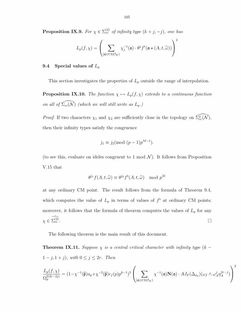
105

Proposition IX.9. For χ ∈ Σ(2)cc of infinity type (k + j,−j), one has

Lp(f, χ) =

∑[a]∈Cl(OK)

χ−1j (a) · θjf [(a ? (A, t, ω))

2

9.4 Special values of Lp

This section investigates the properties of Lp outside the range of interpolation.

Proposition IX.10. The function χ 7→ Lp(f, χ) extends to a continuous function

on all of Σcc(N ) (which we will still write as Lp.)

Proof. If two characters χ1 and χ2 are sufficiently close in the topology on Σ2cc(N ),

then their infinity types satisfy the congruence

j1 ≡ j2(mod (p− 1)pM−1).

(to see this, evaluate on ideles congruent to 1 mod N ). It follows from Proposition

V.15 that

θj1f(A, t, ω) ≡ θj2f [(A, t, ω) mod pM

at any ordinary CM point. The result follows from the formula of Theorem 9.4,

which computes the value of Lp in terms of values of f [ at ordinary CM points;

moreover, it follows that the formula of theorem computes the values of Lp for any

χ ∈ Σ(2)cc .

The following theorem is the main result of this document.

Theorem IX.11. Suppose χ is a central critical character with infinity type (k −

1− j, 1 + j), with 0 ≤ j ≤ 2r. Then

Lp(f, χ)

Ω2(2r−2j)p

= (1−χ−1(p)ap+χ−2(p)εf (p)p

k−1)2

∑[a]∈Cl(OK)

χ−1(a)N(a) · AJF (∆φa)(ωf ∧ ωjAη2r−jA )

2

106

Proof. The proof of the preceding proposition establishes the formula

Lp(f, χ) =

∑[a]∈Cl(OK)

χ−1−1−j(a) · θ−1−jf [(a ? (A, t, ω))

2

.

By definition of Ωp we have (using that the weight of θ−1−jf [ is k − 2− 2j) that

Lp(f, χ)

Ω2(2r−2j)p

=

∑[a]∈Cl(OK)

χ−1−1−j(a) · θ−1−jf [(a ? (A, t, ω))

2

.

Lemma VIII.3 shows that the value of θ−1−j acting on f [ is 1j!gj[ where gj denotes

the jth component of the Coleman primitive for f , which gives

Lp(f, χ)

Ω2(2r−2j)p

=1

j!

∑[a]∈Cl(OK)

χ−1−1−j(a) · θ−1−j gj

[(a ? (A, t, ω))

2

.

By Lemma IX.6 (and a rearrangement of the sum), one can remove the operator [

on gj by dropping an Euler factor:

Lp(f, χ)

Ω2(2r−2j)p

= (1−χ−1(p)ap+χ−2(p)εf (p)p

k−1)2 1

j!

∑[a]∈Cl(OK)

χ−1−1−j(a) · θ−1−j gj(a ? (A, t, ω))

2

.

Now apply Lemma VIII.4 to the Heegner isogeny φa, of degree (Na)2, to attain the

final result.

BIBLIOGRAPHY

107

108

BIBLIOGRAPHY

[Be] Besser, Amnon. CM cycles over Shimura curves. J. Algebraic Geom. 4 (1995), no. 4, 659-691.

[BK] Bloch, Spencer and Kato, Kazuya. L-functions and Tamagawa numbers of motives. TheGrothendieck Festschrift, Vol. I, 333-400, Progr. Math., 86, Birkhauser Boston, Boston, MA,1990.

[BL] Birkenhake, Christina and Lange, Herbert. Complex abelian varieties. Grundlehren der Math-ematischen Wissenschaften. Springer-Verlag, Berlin (2004).

[BDP] Bertolini, M., Darmon, H., and Prasanna, K., Generalised Heegner cycles and p-adic RankinL-series, Duke Math Journal, to appear.

[BDP2] Bertolini, M., Darmon, H., and Prasanna, K., p-adic L-functions and the coniveau filtrationon Chow groups., in progress.

[Br] Brakocevic, Miljan. Anticyclotomic p-adic L-function of central critical Rankin-Selberg L-value.Int. Math. Res. Not. 2011, no. 21.

[Bu] Buzzard, Kevin. Integral models of certain Shimura curves. Duke Math. J. 87 (1997), no. 3,591-612.

[Co] Coleman, Robert. A p-adic Shimura Isomorphism and p-adic periods of modular forms, Con-temporary Mathematics, 165, 1994, 21-51.

[Co2] Coleman, Robert. Reciprocity laws on curves, Compositio Math. 72 (1989), no. 2, 205-235.

[Co3] Coleman, Robert. Torsion Points on Curves and p-Adic Abelian Integrals. Ann. of Math (2)121 (1985), no. 1, 111-168.

[CS] Coates, J., and Sujatha, R. Cyclotomic fields and zeta values. Springer Monographs in Math-ematics. Springer-Verlag, Berlin (2006).

[De] Deligne, P. Equations differentielles a points singuliers reguliers. Lecture Notes in Mathemat-ics, Vol. 163. Springer-Verlag, Berlin-New York (1970).

[Di] Disegni, D. p-adic Heights of Heegner Points on Shimura Curves. Unpublished, available athttp://arxiv.org/abs/1304.5204 (2013).

[Iw] Iwasawa, K. Lectures on p-adic L-functions. Ann. of Math. Studies, Princeton University Press,Princeton. (1972).

[Ka] Katz, N. p-adic properties of modular schemes and modular forms. Modular functions of onevariable, III (Proc. Internat. Summer School, Univ. Antwerp, Antwerp, 1972), pp. 69-190.Lecture Notes in Mathematics, Vol. 350, Springer, Berlin, 1973.

[Ka2] Katz, N. Serre-Tate Local Moduli. Algebraic Surfaces (Orsay 1976-1978), pp. 138-202, LectureNotes in Math., 868, Springer, Berlin-New York (1981).

[Ka3] Katz, N. p-adic L-functions for CM fields. Invent. Math. 49, (1978), 99-297

109

[Kas] Kassaei, Payman. p-adic modular forms over Shimura Curves over Q. Ph. D. thesis. Availableonline.

[KL] Kubota, T. and Leopoldt, H. Eine p-adische Theorie der Zetawert. I. Einfuhrung der p-adischen Dirichletschen L-Funktionen. J. Reine Agnew. Math. 214/215 (1964) 328-339.

[KM] Katz, N. and Mazur, B. Arithmetic moduli of elliptic curves. Annals of Mathematics Studies,108. Princeton University Press, Princeton, NJ, 1985.

[KO] Katz, N., and Oda, T. On the differentiation of de Rham cohomology classes with respect toparameters. J. Math. Kyoto Univ. 8 (1968), 199-213.

[GZ] Gross, B. and Zagier, D., Heegner points and derivatives of L-series, Invent. Math. 84 (1986),no. 2, 225-320.

[Ma] Masdeu, Marc. CM cycles on Shimura curves, and p-adic L-functions. Compositio Mathe-matica, volume 148, issue 04 (2013), pp. 1003-1032.

[Mo] Mori, Andrea. Power series expansions of modular forms and their interpolation properties.Int. J. Number Theory 7 (2011), no. 2, 529-77.

[Morita] Morita, Y. Reduction modulo p of Shimura curves. Hokkaido Mathematical Journal, 10(2) (1981)

[Ne1] Nekovar, Jan. p-adic Abel-Jacobi maps and p-adic heights. In: The Arithmetic and Geometryof Algebraic Cycles (Banff, Canada, 1998), 367 - 379, CRM Proc. and Lect. Notes 24, Amer.Math. Soc., Providence, RI, 2000.

[Ne2] Nekovar, Jan. On the p-adic height of Heegner cycles. Math. Ann. 302 (1995), 609 - 686.

[Pr] Prasanna, K. Integrality of a ratio of Petersson norms and level-lowering congruences. Ann.of Math. (2) 163 (2006), no. 3, 901-967.

[PR] Perrin-Riou, Bernadette. Points de Heegner et derivees de fonctions L p-adiques, Invent.Math. 89 (1987), no. 3, 455-510.

[Ru] Rubin, Karl. p-adic L-functions and rational points on elliptic curves with complex multipli-cation. Invent. math. 107 (1992), no. 2, 323-350.

[Sch] Scholl, A. Motives for modular forms, Invent. Math. 100 (1990), no. 2, 419-430.

[Se] Serre, J.-P. Formes modulaires et fonctions zeta p-adiques. Modular functions of one variable,III (Proc. Internat. Summer School, Univ. Antwerp, Antwerp, 1972), pp. 191-268. Lecture Notesin Mathematics, Vol. 350, Springer, Berlin, 1973.

[Sh] Shimura, Goro. Construction of Class Fields and Zeta Functions of Algebraic Curves. Ann. ofMath. (2) 85 (1967), no. 1, 58-159.

[Sk] Skinner, C. “A converse to a theorem of Gross-Zagier-Kolyvagin.” Online lecture,http://video.ias.edu/jointiaspu/1213/0404-ChristopherSkinner (2013).

[Vi] Arithmetique des algebres de quaternions. Lecture Notes in Mathematics, 800. Springer, Berlin(1980).

[Vo] Voisin, C. Hodge theory and complex algebraic geometry I., trans. Schneps, L. Cambridgestudies in advanced mathematics. Cambridge University Press, Cambridge (2002).

[Wa] Waldspurger, J.-L. Correspondances de Shimura et quaternions. Forum Math. 3 (1991), no.3, 219-307.

110

[We] Weil, Andre. Basic number theory.Grundlehren der Mathematischen Wissenschaften.Springer-Verlag, New York - Berlin (1967).

[YZZ] Yuan, X., Zhang, S., and Zhang, W. The Gross-Zagier Formula on Shimura Curves. Ann.of Math. Studies, Princeton University Press, Princeton. (2013).

[Zh1] Zhang, Shouwu, Heights of Heegner cycles and derivatives of L-series, Invent. Math. 130(1997), no. 1, 99-152.

[Zh2] Zhang, Shouwu, Heights of Heegner points on Shimura Curves, Ann. of Math. (2) 153 (2001),27-147.