ccdteipmA

rpalLm1tstdd

vout

2

NeuroImage 9, 534–544 (1999)Article ID nimg.1998.0425, available online at http://www.idealibrary.com on

1CA

Generalizable Patterns in Neuroimaging:How Many Principal Components?

Lars Kai Hansen,*,1 Jan Larsen,* Finn Årup Nielsen,* Stephen C. Strother,†,\ Egill Rostrup,‡ Robert Savoy,§Nicholas Lange,¶ John Sidtis,\ Claus Svarer,** and Olaf B. Paulson**

*Department of Mathematical Modeling, Technical University of Denmark, Building 321, DK-2800 Lyngby, Denmark; †PET Imaging Service,VA Medical Center, and Department of Radiology, and \Department of Neurology, University of Minnesota, Minneapolis, Minnesota 55455;

‡Danish Center for Magnetic Resonance, Hvidovre Hospital, DK-2650 Hvidovre, Denmark; §Department of Radiology, MassachusettsGeneral Hospital, Charlestown, Massachusetts 02129; ¶McLean Hospital and Harvard Medical School, Belmont, Massachusetts 02178;

and **Neurobiology Research Unit, Rigshospitalet DK-2100, Copenhagen, Denmark

Received June 25, 1998

sltlurdlTviHafilrvafamKta

iPt

perf

Generalization can be defined quantitatively andan be used to assess the performance of principalomponent analysis (PCA). The generalizability of PCAepends on the number of principal components re-ained in the analysis. We provide analytic and test setstimates of generalization. We show how the general-zation error can be used to select the number ofrincipal components in two analyses of functionalagnetic resonance imaging activation sets. r 1999

cademic Press

INTRODUCTION

Principal component analysis (PCA) and the closelyelated singular value decomposition technique areopular tools for analysis of image data sets and arectively investigated in functional neuroimaging (Moel-er and Strother, 1991; Friston et al., 1993, 1995;autrup et al., 1995; Strother et al., 1995, 1996; Bull-ore et al., 1996; Ardekani et al., 1998; Worsley et al.,

997). By PCA the image data set is decomposed inerms of orthogonal ‘‘eigenimages’’ that may lend them-elves to direct interpretation. Principal components,he projections of the image data onto the eigenimages,escribe uncorrelated event sequences in the imageata set.Furthermore, we can capture the most important

ariations in the image data set by keeping only a fewf the high-variance principal components. By suchnsupervised learning we discover hidden, linear rela-ions among the original set of measured variables.

1 To whom correspondence should be addressed. Fax: (145) 4587

c599. E-mail: lkhansen@imm.dtu.dk.

534053-8119/99 $30.00opyright r 1999 by Academic Pressll rights of reproduction in any form reserved.

Conventionally learning problems are divided intoupervised and unsupervised learning. Supervisedearning concerns the identification of functional rela-ionships between two or more variables as in, e.g.,inear regression. The objective of PCA and othernsupervised learning schemes is to capture statisticalelationships, i.e., the structure of the underlying dataistribution. Like supervised learning, unsupervisedearning proceeds from a finite sample of training data.his means that the learned components are stochasticariables depending on the particular (random) train-ng set forcing us to address the issue of generalization:ow robust are the learned components to fluctuationnd noise in the training set, and how well will theyare in predicting aspects of future test data? General-zation is a key topic in the theory of supervisedearning, and significant theoretical progress has beeneported (see, e.g., Larsen and Hansen, 1997). Unsuper-ised learning has not enjoyed the same attention,lthough results for specific learning machines can beound. In Hansen and Larsen (1996) we defined gener-lization for a broad class of unsupervised learningachines and applied it to PCA and clustering by the-means method. In particular we used generalization

o select the optimal number of principal components insmall simulation example.The objective of this paper is to expand on the

mplementation and application of generalization forCA in functional neuroimaging. A brief account of

hese results was presented in Hansen et al. (1997).In what follows we describe a general framework for

arameter estimation on any given data set and thensuing generalization errors associated with this pa-ameterization. We then discuss the application of thisramework to PCA and how the generalization error

an be estimated analytically and empirically. By exam-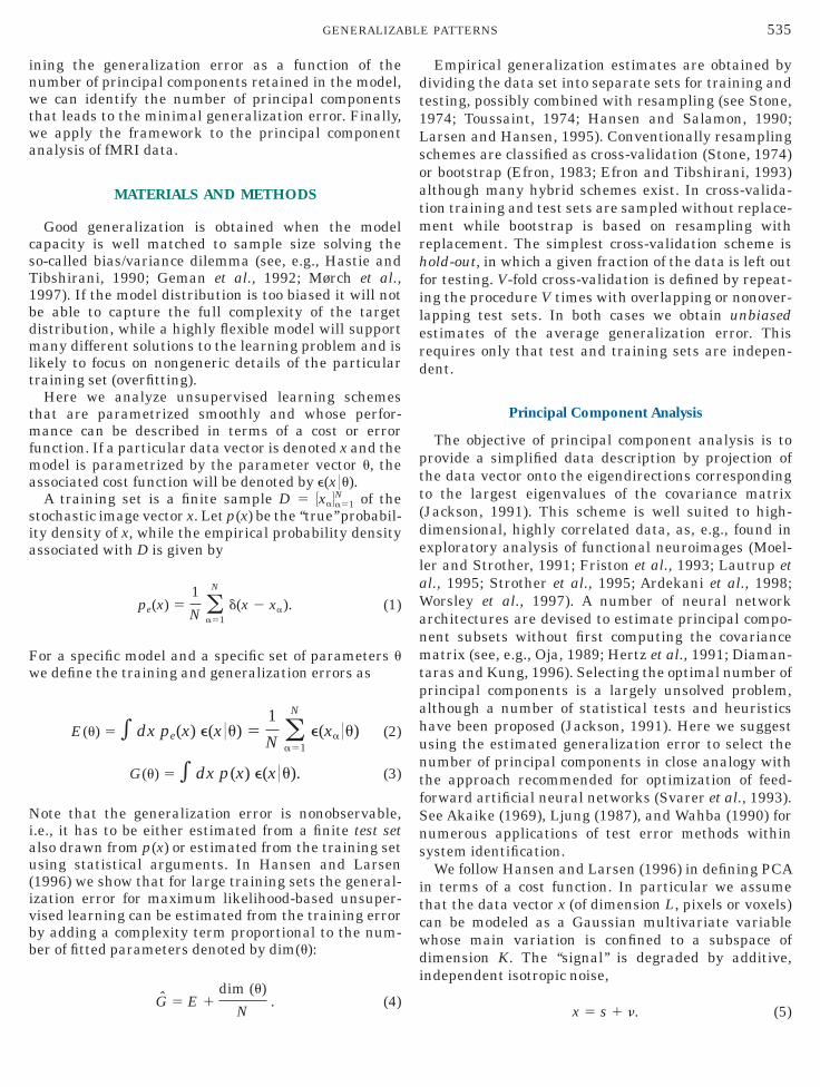

inwtwa

csT1bdmlt

tmfma

sia

Fw

Niau(ivbb

dt1Lsoatmrhfilerd

ptt(delaWanmtpahuntfSns

itcwdi

535GENERALIZABLE PATTERNS

ning the generalization error as a function of theumber of principal components retained in the model,e can identify the number of principal components

hat leads to the minimal generalization error. Finally,e apply the framework to the principal componentnalysis of fMRI data.

MATERIALS AND METHODS

Good generalization is obtained when the modelapacity is well matched to sample size solving theo-called bias/variance dilemma (see, e.g., Hastie andibshirani, 1990; Geman et al., 1992; Mørch et al.,997). If the model distribution is too biased it will note able to capture the full complexity of the targetistribution, while a highly flexible model will supportany different solutions to the learning problem and is

ikely to focus on nongeneric details of the particularraining set (overfitting).

Here we analyze unsupervised learning schemeshat are parametrized smoothly and whose perfor-ance can be described in terms of a cost or error

unction. If a particular data vector is denoted x and theodel is parametrized by the parameter vector u, the

ssociated cost function will be denoted by e(x 0u).A training set is a finite sample D 5 5xa6a51

N of thetochastic image vector x. Let p(x) be the ‘‘true’’ probabil-ty density of x, while the empirical probability densityssociated with D is given by

pe(x) 51

N oa51

N

d(x 2 xa). (1)

or a specific model and a specific set of parameters ue define the training and generalization errors as

E(u) 5 e dx pe(x) e(x 0u) 51

N oa51

N

e(xa 0u) (2)

G(u) 5 e dx p(x) e(x 0u). (3)

ote that the generalization error is nonobservable,.e., it has to be either estimated from a finite test setlso drawn from p(x) or estimated from the training setsing statistical arguments. In Hansen and Larsen1996) we show that for large training sets the general-zation error for maximum likelihood-based unsuper-ised learning can be estimated from the training errory adding a complexity term proportional to the num-er of fitted parameters denoted by dim(u):

G 5 E 1dim (u)

. (4)

N

Empirical generalization estimates are obtained byividing the data set into separate sets for training andesting, possibly combined with resampling (see Stone,974; Toussaint, 1974; Hansen and Salamon, 1990;arsen and Hansen, 1995). Conventionally resamplingchemes are classified as cross-validation (Stone, 1974)r bootstrap (Efron, 1983; Efron and Tibshirani, 1993)lthough many hybrid schemes exist. In cross-valida-ion training and test sets are sampled without replace-ent while bootstrap is based on resampling with

eplacement. The simplest cross-validation scheme isold-out, in which a given fraction of the data is left out

or testing. V-fold cross-validation is defined by repeat-ng the procedure V times with overlapping or nonover-apping test sets. In both cases we obtain unbiasedstimates of the average generalization error. Thisequires only that test and training sets are indepen-ent.

Principal Component Analysis

The objective of principal component analysis is torovide a simplified data description by projection ofhe data vector onto the eigendirections correspondingo the largest eigenvalues of the covariance matrixJackson, 1991). This scheme is well suited to high-imensional, highly correlated data, as, e.g., found inxploratory analysis of functional neuroimages (Moel-er and Strother, 1991; Friston et al., 1993; Lautrup etl., 1995; Strother et al., 1995; Ardekani et al., 1998;orsley et al., 1997). A number of neural network

rchitectures are devised to estimate principal compo-ent subsets without first computing the covarianceatrix (see, e.g., Oja, 1989; Hertz et al., 1991; Diaman-

aras and Kung, 1996). Selecting the optimal number ofrincipal components is a largely unsolved problem,lthough a number of statistical tests and heuristicsave been proposed (Jackson, 1991). Here we suggestsing the estimated generalization error to select theumber of principal components in close analogy withhe approach recommended for optimization of feed-orward artificial neural networks (Svarer et al., 1993).ee Akaike (1969), Ljung (1987), and Wahba (1990) forumerous applications of test error methods withinystem identification.We follow Hansen and Larsen (1996) in defining PCA

n terms of a cost function. In particular we assumehat the data vector x (of dimension L, pixels or voxels)an be modeled as a Gaussian multivariate variablehose main variation is confined to a subspace ofimension K. The ‘‘signal’’ is degraded by additive,ndependent isotropic noise,

x 5 s 1 n. (5)

Tmn

wscet

v

Wt

we

p

w

l

tee atte

536 HANSEN ET AL.

he signal and noise are assumed to be distributed asultivariate Gaussian random variables, s , N (x0, Ss),, N (0, Sn).We assume that Ss is singular, i.e., of rank K , L,hile Sn 5 s2IL, where IL is a L 3 L identity matrix and2 is a noise variance. This ‘‘PCA model’’ corresponds toertain tests proposed in the statistics literature forquality of covariance eigenvalues beyond a certainhreshold (a so-called sphericity test) (Jackson, 1991).

Using well-known properties of Gaussian randomariables we find

x , N (x0, Ss 1 Sn). (6)

e use the negative log-likelihood as a cost function forhe parameters u ; (xo, Ss, Sn),

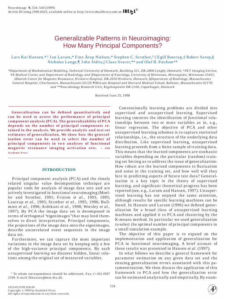
FIG. 1. Data set I. Bias/variance trade-off curves for PCA. The teshe mean, for 10 repetitions of experiment) and the asymptotic estimastimate is asymptotically unbiased. The empirical estimate suggesstimate is too optimistic about the generalizability of the found PC p

e(x 0u) 5 2log p(x 0u), (7)

here p(x 0u) is the p.d.f. of the data given the param-ter vector. Here,

(x 0 x0, Ss, Sn) 51

Î 02p(Ss 1 Sn)0

? exp 12 1

2DxT (Ss 1 Sn)21Dx2 ,

(8)

ith Dx 5 x 2 x0.

Parameter Estimation

Unconstrained minimization of the negative log-ikelihood leads to the well-known parameter estimates

x0 51

N oN

xa, S 51

N oN

(xa 2 x0)(xa 2 x0)ª. (9)

t (*) generalization error estimate (mean 6 the standard deviation ofThe empirical test error is an unbiased estimate, while the analyticaln optimal PCA with K 5 8 components. Note that the asymptoticrns.

t sete.ts a

a51 a51

SwLuscl

Tcc

h

a

S

Ts

Faa are

537GENERALIZABLE PATTERNS

Our model constraint involved in the approximation5 Ss 1 s2IL is implemented as follows. Let S 5 SLSª,here S is an orthogonal matrix of eigenvectors and5 diag ([l1, . . . ,lL]) is the diagonal matrix of eigenval-

es li ranked in decreasing order. By fixing the dimen-ionality of the signal subspace, K, we identify theovariance matrix of the subspace spanned by the Kargest PCs by

SK 5 S · diag([l1, . . . , lK, 0, . . . , 0]) · Sª. (10)

he noise variance is subsequently estimated so as toonserve the total variance (viz., the trace of theovariance matrix),

s2 51

Trace [S 2 SK ], (11)

FIG. 2. Data set I. Eigenimages corresponding to the nine most siig. 1 suggests that the optimal PCA contains eight components. Amoctivation in the right hemisphere corresponding to areas associatedctivation with a possible interpretation as the supplementary motor

L 2 K c

ence

Sn 5 s2IL (12)

nd

ˆs 5 S · diag

? ([l1 2 s2, . . . , lK 2 s2, 0, . . . , 0]) · Sª.(13)

his procedure is maximum likelihood under the con-traints of the model.

Estimating the PCA Generalization Error

When the training set for an adaptive system be-

cant principal components. The unbiased generalization estimate inhe generalizable patterns we find in the sixth component, PC 6, focalith the primary motor cortex. Also there is a trace of a focal centrala.

gnifing t

w

omes large relative to the number of fitted parameters

tettstswLleeoef

w

vo[wttL

cttrl1s

538 HANSEN ET AL.

he fluctuations of these parameters decrease. Thestimated parameters of systems adapted on differentraining sets will become more and more similar as theraining set size increases. In fact we can show formoothly parametrized algorithms that the distribu-ion of these parameters—induced by the randomelection of training sets—is asymptotically Gaussianith a covariance matrix proportional to 1/N (see, e.g.,jung, 1987). This convergence of parameter estimates

eads to a similar convergence of their generalizationrrors. Hence, we may use the average generalizationrror (for identical systems adapted on different samplesf N ) as an asymptotic estimate of the generalizationrror of a specific realization. Details of such analysis

FIG. 3. Data set I. Top: The ‘‘raw’’ time course of principal comovariance matrix); the offset square wave indicates the time courseapping at time intervals at which this function is high. Middle: Smooo the activation. Note that both the delay and the form of the respoeference sequence and the principal component (unsmoothed); the doevel for rejection of a white noise null hypothesis. The significance le996). 1/P 5 1000 random permutations of the principal componenymmetric extremal values used as thresholds for the given P value.

or PCA can be found in Hansen and Larsen (1996),

here we derived the relation

G(u) < E(u) 1dim(u)

N, (14)

alid in the limit as dim (u/N ) = 0. The dimensionalityf the parametrization depends on the number, K [1, L], of principal components retained in the PCA. Ase estimate the (symmetric) signal covariance matrix,

he L-dimensional vector x0 and the noise variance s2,he total number of estimated parameters is dim(u) 5

1 1 1 K(2L 2 K 1 1)/2.

nent 6 (projection of the image sequence onto eigenimage 6 of thehe binary finger opposition activation. The subject performed fingerd principal component with a somewhat more interpretable responsevary from run to run. Bottom: The cross-correlation function of theash horizontal curves indicate the symmetric P 5 0.001 significance

l has been estimated using a simple permutation test (Holmes et al.,equence were cross-correlated with the reference function and the

poof tthenset–dvet s

In real world examples facing limited data sets we

gmsot

E

G

we

tcNma

wnt

gtw ot

539GENERALIZABLE PATTERNS

enerally prefer to estimate the generalization error byeans of resampling. For a particular split of the data

et we can use the explicit form of the distribution tobtain expressions for the training and test errors inerms of the estimated parameters,

51

2log 02p(Ss 1 Sn) 0

11

2Trace [(Ss 1 Sn)21 Strain]

(15)

ˆtestset 5

1

2log 02p(Ss 1 Sn) 0

11

2Trace [(Ss 1 Sn)21 Stest],

(16)

here the covariance matrices, Strain and Stest, are

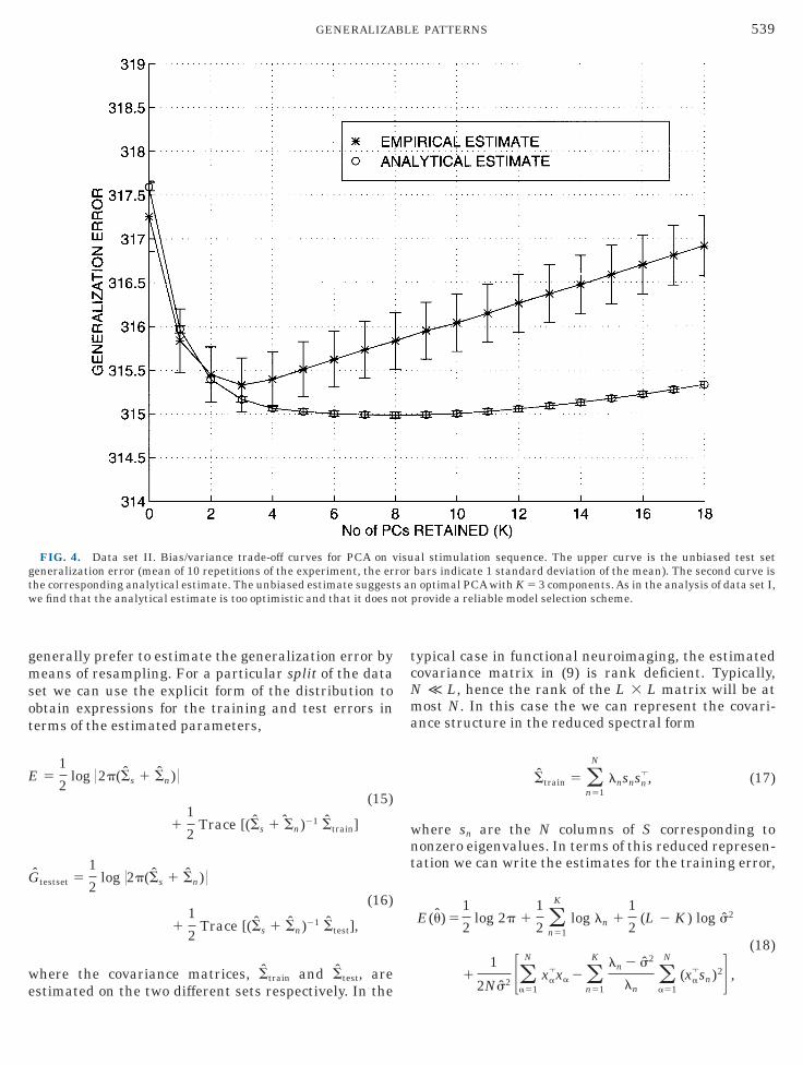
FIG. 4. Data set II. Bias/variance trade-off curves for PCA on veneralization error (mean of 10 repetitions of the experiment, the erhe corresponding analytical estimate. The unbiased estimate suggeste find that the analytical estimate is too optimistic and that it does n

stimated on the two different sets respectively. In the

ypical case in functional neuroimaging, the estimatedovariance matrix in (9) is rank deficient. Typically,9 L, hence the rank of the L 3 L matrix will be atost N. In this case the we can represent the covari-

nce structure in the reduced spectral form

Strain 5 on51

N

lnsnsnª, (17)

here sn are the N columns of S corresponding toonzero eigenvalues. In terms of this reduced represen-ation we can write the estimates for the training error,

E(u) 51

2log 2p 1

1

2 on51

K

log ln 11

2(L 2 K ) log s2

11

2Ns2 3oa51

N

xaªxa 2 o

n51

K ln 2 s2

lnoa51

N

(xaªsn)24 ,

(18)

al stimulation sequence. The upper curve is the unbiased test setbars indicate 1 standard deviation of the mean). The second curve isoptimal PCA with K 5 3 components. As in the analysis of data set I,

provide a reliable model selection scheme.

isurors an

af

Teda

itKemsttum

athrc

540 HANSEN ET AL.

nd similarly the estimate of the generalization erroror a test set of Ntest data vectors will be

G(u) 51

2log 2p 1

1

2 on51

K

log ln

11

2(L 2 K ) log s2 1

1

2Ntests2

? 3ob51

Ntest

xbªxb 2 o

n51

K ln 2 s2

lnob51

Ntest

(xbªsn)24 .

(19)

he nonzero eigenvalues and their eigenvectors can,.g., be found by singular value decomposition of theata matrix X ; [xa]. In Eqs. (18) and (19) we havessumed zero mean signals, x0 5 0, for simplicity.

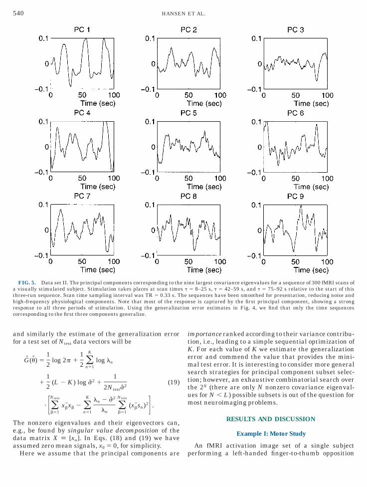
FIG. 5. Data set II. The principal components corresponding to thvisually stimulated subject. Stimulation takes places at scan time

hree-run sequence. Scan time sampling interval was TR 5 0.33 s. Tigh-frequency physiological components. Note that most of the resesponse to all three periods of stimulation. Using the generalizaorresponding to the first three components generalize.

Here we assume that the principal components are p

mportance ranked according to their variance contribu-ion, i.e., leading to a simple sequential optimization of. For each value of K we estimate the generalizationrror and commend the value that provides the mini-al test error. It is interesting to consider more general

earch strategies for principal component subset selec-ion; however, an exhaustive combinatorial search overhe 2N (there are only N nonzero covariance eigenval-es for N , L) possible subsets is out of the question forost neuroimaging problems.

RESULTS AND DISCUSSION

Example I: Motor Study

An fMRI activation image set of a single subject

ne largest covariance eigenvalues for a sequence of 300 fMRI scans of5 8–25 s, t 5 42–59 s, and t 5 75–92 s relative to the start of thissequences have been smoothed for presentation, reducing noise andse is captured by the first principal component, showing a strongerror estimates in Fig. 4, we find that only the time sequences

e nis thepon

tion

erforming a left-handed finger-to-thumb opposition

tlnpat3rtslsagv

ctb

tgwtb

Edspvs(mAaaB

ce

541GENERALIZABLE PATTERNS

ask was acquired. Multiple runs of 72 2.5-s (24 base-ine, 24 activation, 24 baseline) whole-brain echo pla-ar scans were aligned, and an axial slice throughrimary motor cortex and the supplementary motorrea of 42 3 42 voxels (3.1 3 3.1 3 8 mm) was ex-racted. Of a total of 624 scans, training sets of size N 500 were drawn at random and for each training set theemaining independent set of 324 scans was used asest set. PCA analyses were carried out on the traininget. We used Eq. (19) to compute the average negativeog-likelihood on the test set using the covariancetructure estimated on the training sets and Eqs. (4)nd (18) to compute the analytical estimate of theeneralization error. Both estimates were then plottedersus size of the PCA subspace; see Fig. 1.Inspection of the test set curve suggests a model

omprising eight principal components. We note thathe analytical estimate is too optimistic, presumably

FIG. 6. Data set II. Covariance eigenimages corresponding torresponding to the dominating first PC is focused in visual areas.igenimages corresponding to the first three components generalize.

ecause the sample is not large enough for the asymp- o

otic results to hold. It underestimates the level of theeneralization error and points to an optimal modelith more than 20 components which—as measured by

he unbiased estimate—has a generalization error asad as a model with one or two components.The covariance eigenimages are shown in Fig. 2.

igenimages corresponding to components 1–5 areominated by signal sources that are highly localizedpatially (hot spots comprising one to four neighborixels). It is compelling to defer these as confoundingascular signal sources. Component 6, however, has aomewhat more extended hot spot in the contralateralright hemisphere) motor area. In Fig. 3 we provide aore detailed temporal analysis of this signal source.t the top the ‘‘raw’’ principal component sequence isligned with the binary reference function encoding thectivation state (high, finger opposition; low, rest).elow, in the center, we give a low-pass filtered version

he nine most significant principal components. The eigenimageng the bias/variance trade-off curves in Fig. 4, we find that only the

o tUsi

f the principal component sequence. The smoothed

ctscasfsswwiwc(ot

w

3ap5rwpctsbahbctrves

afccv4r

542 HANSEN ET AL.

omponent shows a definite response to the activation,hough with some randomness in the actual delay andhape of the response. At the bottom we plot the cross-orrelation function between the on/off reference functionnd the unsmoothed signal. The cross-correlation functionhows the characteristic periodic sawtooth shape resultingrom correlation of a square-wave signal with a delayedquare wave. The horizontal dash–dot curves are theymmetric P 5 0.001 intervals for significant rejection of ahite noise null hypothesis. These significance curvesere computed as the extremal values after cross-correlat-

ng 1000 time-index permutations of the reference functionith the actual principal component sequence. The signifi-

ance level has not been corrected for multiple hypothesesBonferroni). Such a correction depends in a nontrivial wayn the detailed specification of the null and is not relevanto the present exploratory analysis.

Example II: Visual Stimulation

A single slice holding 128 3 128 pixels was acquired

FIG. 7. Data set II. Cross-correlation analyses based on a referencnd the value 11 for scans taken during stimulation. Each panel shunction for times t [ [2100 s, 100s]. The dotted horizontal curves aross-correlation. These curves are computed in a manner similar toomponent sequence were cross-correlated with the reference functioalue. The test has not been corrected for simultaneous test of multip) only component 1 shows significant correlation with the activationeference function delayed by t < 10 scans corresponding to 3.3 s.

ith a time interval between successive scans of TR 5 s

33 ms. Visual stimulation in the form of a flashingnnular checkerboard pattern was interleaved witheriods of fixation. A run consisting of 25 scans of rest,0 scans of stimulation, and 25 scans of rest wasepeated 10 times. For this analysis a contiguous maskas created with 2440 pixels comprising the essentialarts of the slice including the visual cortex. Principalomponent analyses were performed on a subset ofhree runs (N 5 300, runs 4–6) with increasing dimen-ionality of the signal subspace. Since the time intervaletween scans was much shorter than in the previousnalysis temporal correlations were expected on theemodynamic time scale (5–10 s). Hence, we used alock-resampling scheme: the generalization error isomputed on a randomly selected ‘‘hold-out’’ contiguousime interval of 50 scans (,16.7 s). The procedure wasepeated 10 times with different generalization inter-als. In Fig. 4 we show the estimated generalizationrrors as function of subspace dimension. The analysisuggests an optimal model with a three-dimensional

me function taking the value 21 at times corresponding to rest scanss the cross-correlation of the principal component and the reference

5 0.001 levels in a nonparametric permutation test for significantlmes et al. (1996): 1/P 5 1000 random permutations of the principald the (two-sided) extremal values used as thresholds for the given P

ypotheses (Bonferroni). Of the three generalizable patterns (c.f., Fig.erence function. The first component is maximally correlated with a

e tiowre PHo

n anle href

ignal subspace. In line with our observation for data

sg

5mcFafcatpttpm

ssPfisstrir

pretcaPsGbgpa

tctlceit

chN‘

A

A

B

D

E

E

F

F

G

H

H

H

H

H

H

J

L

L

543GENERALIZABLE PATTERNS

et I the analytic estimate is too optimistic about theeneralizability of the high-dimensional models.The first nine principal components are shown in Fig.

; all curves have been low-pass filtered to reduceeasurement noise and physiological signals. The first

omponent picks up a pronounced activation signal. Inig. 6 we show the corresponding covariance eigenim-ges. The first component is dominated by an extendedocal activity in primary visual cortex (V1). The thirdomponent, also included in the optimal model, showsn interesting temporal localization, suggesting thathis mode is a kind of ‘‘generalizable correction’’ to therimary response in the first component, this correc-ion being active mainly in the final third run. Spa-ially, the third component is also quite localized,icking up signals in three spots anterior to the pri-ary visual areas.In Fig. 7 we have performed cross-correlation analy-

es of all of the nine most variant principal componentequences. The horizontal dash–dot curves indicate

5 0.001 significance intervals as above. While therst component stands out clearly with respect to thisignificance level, the third component does not seemignificantly cross-correlated with the reference func-ion in line with the remarks above. This componentepresents a minor correction to the primary responsen the first component active mainly during the thirdun of the experiment.

CONCLUSION

We have presented an approach for optimization ofrincipal component analyses on image data withespect to generalization. Our approach is based onstimating the predictive power of the model distribu-ion of the our PCA model. The distribution is aonstrained Gaussian compatible with the generallyccepted interpretation of PCA, namely that we can useCA to identify a low-dimensional salient signal sub-pace. The model assumes a Gaussian signal andaussian noise appropriate for an exploratory analysisased on covariance. We proposed two estimates ofeneralization. The first is based on resampling androvides an unbiased estimate, while the second is annalytical estimate which is asymptotically unbiased.The usefulness of the approach was demonstrated on

wo functional magnetic resonance data sets. In bothases we found that the model with the best generaliza-ion ability picked up signals that were strongly corre-ated with the activation reference sequence. In bothases we also found that the analytical generalizationstimate was too optimistic about the level of general-zation. Furthermore, the optimal model suggested by

his method was severely overparametrized.

ACKNOWLEDGMENTS

The authors thank the anonymous reviewers for constructiveomments that improved the presentation of this paper. This projectas been funded by The Danish Research Councils Interdisciplinaryeuroscience Project and the Human Brain Project P20 MH57180

‘Spatial and Temporal Patterns in Functional Neuroimaging.’’

REFERENCES

kaike, H. 1969. Fitting autoregressive models for prediction. Ann.Inst. Stat. Mat. 21:243–247.rdekani, B., Strother, S. C., Anderson, J. R., Law, I., Paulson, O. B.,Kanno, I., and Rottenberg, D. A. 1998. On detection of activationpatterns using principal component analysis. In Proceedings ofBrainPET’97: Quantitative Functional Brain Imaging with Posi-tron Emission Tomography (R. E. Carson et al., Eds.). AcademicPress, San Diego, in press..

ullmore, E. T., Rabe-Hasketh, S., Morris, R. G., Williams, S. C. R.,Gregory, L., Gray, J. A., and Brammer, M. J. 1996. Functionalmagnetic resonance image analysis of a large-scale neurocognitivenetwork. NeuroImage 4:16–33.iamantaras, K. I., and Kung, S. Y. 1996. Principal ComponentNeural Networks: Theory and Applications. Wiley, New York.

fron, B. 1983. The jackknife, bootstrap and other resampling plans.SIAM Monogr. 38. CBMS-NSF, Philadelphia.

fron, B., and Tibshirani, R. J. 1993. An Introduction to the Boot-strap. Chapman & Hall, New York.

riston, K. J., Frith, C. D., Liddle, P. F., and Frackowiak, R. S. J.1993. Functional connectivity: The principal-component analysisof large (PET) data sets. J. Cereb. Blood Flow Metab. 13:5–14.

riston, K. J., Frith, C. D., Frackowiak, R. S. J., and Turner, R. 1995.Characterizing dynamic brain responses with fMRI: A multivariateapproach. NeuroImage 2:166–172.eman, S., Bienenstock, E., and Doursat, R. 1992. Neural networksand the bias/variance dilemma. Neural Comput. 4:1–58.ansen, L. K., and Salamon, P. 1990. Neural network ensembles.IEEE Trans. Pattern Anal. Mach. Intell. 12:993–1001.ansen, L. K., and Larsen, J. 1996. Unsupervised learning andgeneralization. In Proceedings of the IEEE International Confer-ence on Neural Networks 1996, Vol. 1, pp. 25–30. Washington, DC.ansen, L. K., Nielsen, F. A. A., Toft, P., Strother, S. C., Lange, N.,Morch, N., Svarer, C., Paulson, O. B., Savoy, R., Rosen, B., Rostrup,E., Born, P. 1997. How many principal components? Third Interna-tional Conference on Functional Mapping of the Human Brain,Copenhagen, 1997. NeuroImage 5:474.astie, T., and Tibshirani, R. 1990. Generalized Additive Models.Chapman & Hall, London.ertz, J., Krogh, A., and Palmer, R. G. 1991. Introduction to theTheory of Neural Computation. Addison–Wesley, Redwood City,CA.olmes, A. P., Blair, R. C., Watson, J. D. G., and Ford, I. 1996.Non-parametric analysis of statistic images from functional map-ping experiments. J. Cereb. Blood Flow Metab. 16:7–22.

ackson, J. E. 1991. A User’s Guide to Principal Components. Wiley,New York.

arsen, J., and Hansen, L. K. 1995. Empirical generalization assess-ment of neural network models. In Proceedings of the IEEEWorkshop on Neural Networks for Signal Processing V, (F. Girosi, J.Makhoul, E. Manolakos, and E. Wilson, Eds.), pp. 30–39. Piscat-away, NJ.

arsen, J., and Hansen, L. K. 1997. Generalization: The hidden

agenda of learning. In The Past, Present, and Future of Neural

L

L

M

M

O

S

S

S

S

T

W

W

544 HANSEN ET AL.

Networks for Signal Processing (J.-N. Hwang, S. Y. Kung, M.Niranjan, and J. C. Principe, Eds.), IEEE Signal ProcessingMagazine, November, pp. 43–45.

autrup, B., Hansen, L. K., Law, I., Mørch, N., Svarer, C., andStrother, S. C. 1995. Massive weight sharing: A cure for extremelyill-posed problems. In Supercomputing in Brain Research: FromTomography to Neural Networks (H. J. Herman et al., Eds.), pp.137–148. World Scientific, Singapore.

jung, L. 1987. System Identification: Theory for the User. PrenticeHall, Englewood Cliffs, NJ.oeller, J. R., and Strother, S. C. 1991. A regional covarianceapproach to the analysis of functional patterns in positron emissiontomographic data. J. Cereb. Blood Flow Metab. 11:A121–A135.ørch, N., Hansen, L. K., Strother, S. C., Svarer, C., Rottenberg,D. A., Lautrup, B., Savoy, R., and Paulson, O. B. 1997. Nonlinearversus linear models in functional neuroimaging: Learning curvesand generalization crossover. In Information Processing in MedicalImaging (J. Duncan et al., Eds.), Lecture Notes in ComputerScience, Vol. 1230, pp. 259–270. Springer-Verlag, Berlin/New York.ja, E. 1989. Neural networks, principal components, and subspaces.Int. J. Neural Syst. 1:61–68.

tone, M. 1974. Cross-validatory choice and assessment of statistical

predictors. J. R. Stat. Soc. B 36:111–147.

trother, S. C., Anderson, A. R., Schaper, K. A., Sidtis, J. J., Woods,R. P., and Rottenberg, D. A. 1995. Principal component analysisand the scaled subprofile model compared to intersubject averag-ing of a statistical parametric mapping. I. ‘‘Functional connectivity’’of the human motor system studied with [15O]PET. J. Cereb. BloodFlow Metab. 15:738–775.

trother, S. C., Lange, N., Savoy, R. L., Anderson, J. R., Sidtis, J. J.,Hansen, L. K., Bandettini, P. A., O’Craven, K., Rezza, M., Rosen,B. R., and Rottenberg, D. A. 1996. Multidimensional state spacesfor fMRI and PET activation studies. Neuroimage 2(Pt 2):98.

varer, C., Hansen, L. K., and Larsen, J. 1993. On design andevaluation of tapped-delay neural network architectures. In Pro-ceedings of the 1993 IEEE International Conference on NeuralNetworks (H. R. Berenji et al., Eds., Vol. 1, pp. 46–51. IEEE ServiceCenter, Piscataway, NJ.

oussaint, G. T. 1974. Bibliography on estimation of misclassifica-tion. IEEE Trans. Inf. Theor. 20:472–479.ahba, G. 1990. Spline models for observational data. In CBMS-NSFRegional Conference Series in Applied Mathematics, Vol. 59. SIAM,Philadelphia.orsley, K. J., Poline, J.-B., Friston, K. J., and Evans, A. C. 1997.Characterizing the response of PET and fMRI data using multivar-

iate linear models (MLM). NeuroImage 6:305–319.