
General Solution of the Incompressible, Potential … Solution of the Incompressible, Potential Flow...
16
General Solution of the Incompressible, Potential Flow Equations CHAPTER 3 Developing the basic methodology for obtaining the elementary solutions to potential flow problem. Linear nature of the potential flow problem, the differential equation does not have to be solved individually for flow fields having different geometry at their boundaries. Instead, the elementary solutions will be distributed in a manner that will satisfy each individual set of geometrical boundary conditions. 1 - !"# 3.1 Statement of the Potential Flow Problem The continuity equation for incompressible and irrotational The velocity component normal to the body’s surface and to other solid boundaries must be zero, and in a body-fixed coordinate system ∇Φ is measured in a frame of reference attached to the body. The disturbance created by the motion should decay far (r →∞) from the body where r = (x, y, z) and v is the relative velocity between the undisturbed fluid in V and the body (or the velocity at infinity seen by an observer moving with the body). 2
Transcript of General Solution of the Incompressible, Potential … Solution of the Incompressible, Potential Flow...
General Solution of the
Incompressible, Potential Flow
Equations
CHAPTER 3
Developing the basic methodology for obtaining the elementary solutions
to potential flow problem.
Linear nature of the potential flow problem, the differential equation
does not have to be solved individually for flow fields having different
geometry at their boundaries.
Instead, the elementary solutions will be distributed in a manner that will
satisfy each individual set of geometrical boundary conditions.
1 ������� ���- ������� ������� ����� ������
���� ���� ��� !"��#
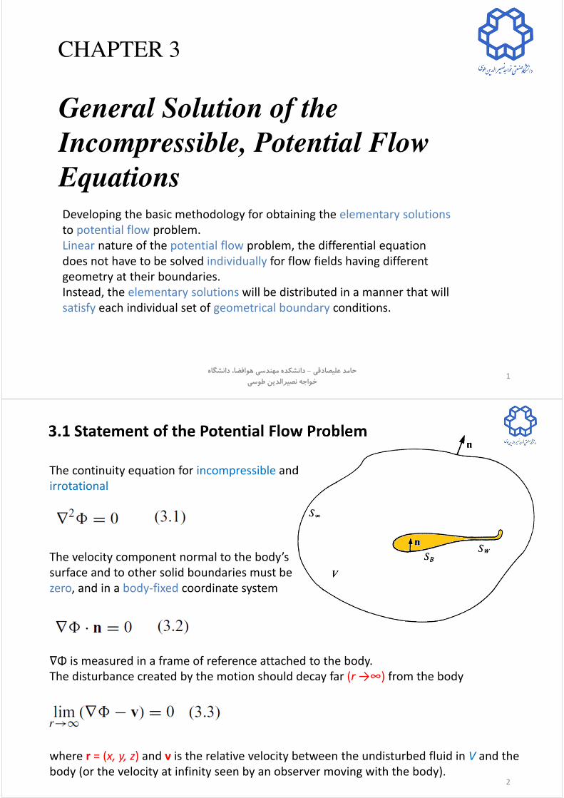
3.1 Statement of the Potential Flow Problem
The continuity equation for incompressible and
irrotational
The velocity component normal to the body’s
surface and to other solid boundaries must be
zero, and in a body-fixed coordinate system
∇Φ is measured in a frame of reference attached to the body.
The disturbance created by the motion should decay far (r →∞) from the body
where r = (x, y, z) and v is the relative velocity between the undisturbed fluid in V and the
body (or the velocity at infinity seen by an observer moving with the body).2

3.2 The General Solution, Based on Green’s Identity
The divergence theorem Eq. (1.20)
q Replace by
where Φ1 and Φ2 are two scalar functions of position
one of Green’s identities
Solving Laplace’s equation for the velocity
potential for an arbitrary body with one of
Green’s identities
Volume integral Surface integral
Wake Model
3
3.2 The General Solution, 3D (Continue…)
Φ: potential of the flow of interest in V
r : distance from a point P(x, y, z)
Let us set:
Case I : Point P is outside of V
Φ1 and Φ2 satisfy Laplace’s equation in V
Eq. (3.4)
Case I : Point P is outside of V
Case II : Point P is inside V
Case III: Point P lies on the boundary (for Example SB)
4

3.2 The General Solution, 3D (Continue…)
Case II : Point P is inside the region V
Φ1 and Φ2 satisfy Laplace’s equation in V with
excluded small sphere of radius ϵ
Eq. (3.4)
Spherical coordinate
system at P
5
3.2 The General Solution, 3D (Continue…)
Potential and its derivatives are well-
behaved functions and therefore do
not vary much in the small sphere
Eq. (3.6b)
This formula gives the value of Φ(P) at any point in the flow, within the region V, in
terms of the values of Φ and ∂Φ /∂n on the boundaries S
6

3.2 The General Solution, 3D (Continue…)
Case III: Point P lies on the boundary SB
Integration around the hemisphere with radius ϵ
Eq. (3.7)
Flow of interest occurs inside the boundary of SB
Φi : internal potential
For this flow the point P (which is in the region V)
is exterior to SB
Eq. (3.6)
n points outward from SB 7
3.2 The General Solution, 3D (Continue…)
Eq. (3.7) + Eq. (3.7b)
Combination of Inner and outer Potential
The contribution of the S∞ This potential depends on the
selection of the coordinate sys.
for example, in an inertial
system where the body moves
through an otherwise stationary
fluid Φ∞ =Constant
the wake surface is assumed to be thin, such that ∂Φ /∂n is continuous across
it (which means that no fluid-dynamic loads will be supported by the wake)
8

3.2 The General Solution, 3D (Continue…)
Determining values of Φ and
∂Φ /∂n on the boundaries Eq. (3.7) or Eq. (3.10)
Reduced to
Doublet:
Source:
Eq. (3.10)
Doublet strength μ is potential difference between the upper and lower wake surfaces
(that is, if the wake thickness is zero, then μ = −∆Φ on SW)
9
3.2 The General Solution, 3D (Continue…)
n .∇∇∇∇ by ∂/∂nEq. (3.13)
Source and doublet solutions decay as r →∞ and automatically fulfill the boundary
condition of Eq. (3.3) (where v is the velocity due to Φ∞)
Determining the strength of
distribution of doublets and
source on surface
To find the velocity
potential in the region V
In Eq. (3.13) non-unique combination of sources and doublets for a particular problem
Choice based on the physics of the problem
source term on SB vanishes and only the
doublet distribution remains
doublet term on SB vanishes10

3.2 The General Solution, 2D (Continue…)
In the two-dimensional case
Source Potential
Eq. (3.6b)
Eq. (3.7)
If the point P lies on the boundary SB
If the point P is inside SB
Eq. (3.7b)
Eq. (3.13a)
Note: ∂/∂n is the orientation of the
doublet as will be illustrated in later
and that the wake model SW in the
steady, two-dimensional lifting case is
needed to represent a discontinuity in
the potential Φ
11
3.3 Summary: Methodology of Solution
In 3D Eq. (3.13)
In 2D Eq. (3.17)
General approach to
solution of incompressible
potential flow problems
Distributing elementary
solutions (sources and
doublets) on the problem
boundaries (SB, SW).
∇Φ2 = 0at r →∞
at r=0
Satisfy B.C. Eq. (3.3)
Velocity becomes singular,
basic elements are called
singular solutions
Integration of basic
solutions over any surface
S containing these
singularity elements
finding appropriate
singularity element
distribution over some
known boundaries
reduced to
for general solution
B.C. Eq. (3.2) will be fulfilled
12

3.4 Basic Solution: Point Source 3D
One of the two basic solutions presented in
Eq. (3.13)
Point source element placed at the origin of a
spherical coordinate system
Velocity field with a radial component only
Velocity in the radial direction decays with the
rate of 1/r2 and is singular at r = 0
13
3.4 Basic Solution: Point Source 3D (Continue)
The volumetric flow rate through a spherical
surface of radius r
Note: this introduction of fluid at the source violates the conservation of mass;
therefore, this point must be excluded from the region of solution
If the point element is located at a point r0
σ : Volumetric rate
positive σ : Source
negative σ : Sink
14

3.4 Basic Solution: Point Source 3D (Continue)
The Cartesian form
The velocity components
15
3.4 Basic Solution: Point Source 3D (Continue)
The basic point element (Eq. (3.24)) can be integrated over a line l, a surface S, or a
volume V to create corresponding singularity elements
Note: σ represents the source strength per unit length, area, and volume
The velocity components induced by these distributions can be obtained by
differentiating the corresponding potentials
16
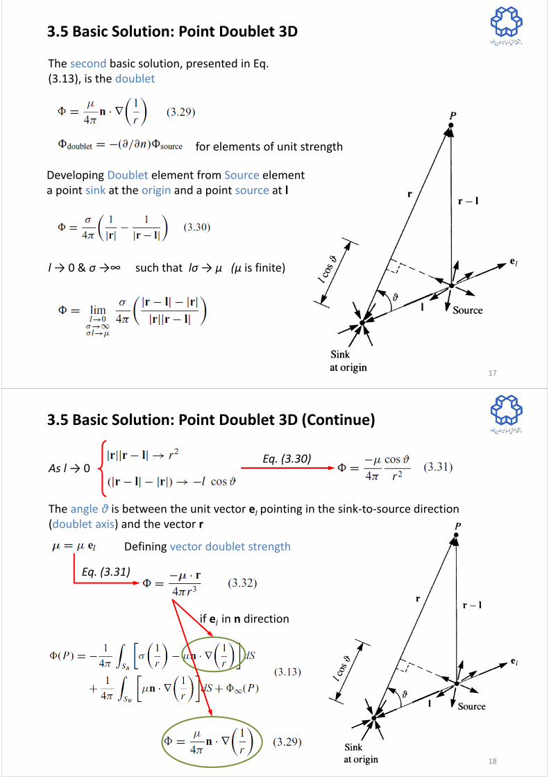
3.5 Basic Solution: Point Doublet 3D
The second basic solution, presented in Eq.
(3.13), is the doublet
for elements of unit strength
Developing Doublet element from Source element
a point sink at the origin and a point source at l
l → 0 & σ →∞ such that lσ → μ (μ is finite)
17
3.5 Basic Solution: Point Doublet 3D (Continue)
As l → 0
The angle θ is between the unit vector el pointing in the sink-to-source direction
(doublet axis) and the vector r
Eq. (3.30)
Defining vector doublet strength
Eq. (3.31)
if el in n direction
18
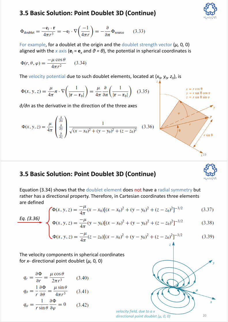
3.5 Basic Solution: Point Doublet 3D (Continue)
For example, for a doublet at the origin and the doublet strength vector (μ, 0, 0)
aligned with the x axis (el = ex and θ = ϑ), the potential in spherical coordinates is
The velocity potential due to such doublet elements, located at (x0, y0, z0), is
∂/∂n as the derivative in the direction of the three axes
19
3.5 Basic Solution: Point Doublet 3D (Continue)
Equation (3.34) shows that the doublet element does not have a radial symmetry but
rather has a directional property. Therefore, in Cartesian coordinates three elements
are defined
Eq. (3.36)
The velocity components in spherical coordinates
for x- directional point doublet (μ, 0, 0)
velocity field, due to a x
directional point doublet (μ, 0, 0) 20

3.5 Basic Solution: Point Doublet 3D (Continue)
The velocity components in Cartesian coordinates
for x- directional point doublet (μ, 0, 0)
Differentiating Eq. (3.37)
This basic point element can be integrated over a line l, a surface S, or a volume V to
create the corresponding singularity elements (for (μ, 0, 0))
21
3.6 Basic Solution: Polynomials 3D
22
Laplace’s equation
is a 2nd order PDE
linear function
can be a solution
velocity components
Where U∞, V∞, and W∞ are constant velocity components in the x, y, and z directions.
the velocity potential due a constant free-stream flow in the x direction is
and in general

3.6 Basic Solution: Polynomials 3D (Continue)
23
to satisfy
Laplace’s Eq
Additional polynomial solutions can be sought
A, B, and C should be constants. There are numerous combinations of constants that
will satisfy this condition.stagnation flow
against a wall
At origin x= z = 0, velocity components u = w = 0
stagnation point
Streamline equation (Eq. 1.6a)
3.7 2D Version of the Basic Solutions (Source)
24
qr ≠ 0
qϑ = 0
qφ = 0
At 3D source
element
qr ≠ 0
qϑ = 0
At 2D source
element
Satisfing the continuity equation (Eq. (1.35))
For Irrotational
flow
qr function of r only
qr = qr(r)
σ: area flow rate passing across a circle of radius r.
velocity components for a source element at the origin:
Integrating
Velocity Potential
C Can be set zero
σ: strength of the source
r = 0 is a singular point and must be
excluded from region of solution

3.7 2D Version of the Basic Solutions (Source)
25
In Cartesian coordinates with source located at (x0, z0)
In 2D stream fuction Eqs. (2.80a,b)
Integrating
Integr. const.= zero
Velocity Potential Stream Function
3.7 2D Version of the Basic Solutions (Doulet)
26
2D doublet can be obtained by a point source and a point sink approach each other
3D Doublet
Eq. (3.32)
Eq. (3.33)
Replacing the source strength by μ & with n in the x direction
Eq. (3.66)
The Velocity field by differentiating the velocity potential

3.7 2D Version of the Basic Solutions (Doulet)
27
The velocity potential in Cartesian, doublet at the point (x0, z0)
The velocity components
Deriving the stream function for this doublet element
Integrating
Integr. const.= zero
Note: a similar doublet element where μ = (0,μ) can be derived by using Eq. (3.66)
3.8 Basic Solution: Vortex
28
In 2D Point Vortex Velocity Potential & Velocity Field
In 3D Vortex Filament Velocity Field by Biot–Savart Law
A singularity element with only a tangential velocity component
Velocity components:
Substitution in continuity
equation (Eq. (1.35))
For irrotational flow
Integrating with respect to r

Note: Γ is positive in clockwise
The velocity field:
The tangential velocity component decays at a rate of 1/r
The velocity potential for a vortex element at the origin
3.8 Basic Solution: Vortex (Continue)
29
Calculating A by using the definition of the circulation
integration
Integrating around a vortex we do find vorticity concentrated at a zero-area point, but
with finite circulation. if we integrate q . dl around any closed curve in the field (not
surrounding the vortex) the value of the integral will be zero.
The vortex is a solution to the Laplace equation and results in an irrotational flow,
excluding the vortex point itself.
In Cartesian coordinates for a vortex located at (x0, z0)
Deriving stream function for 2D vortex located at the origin, in x–z or (r– θ) plane
The streamlines where Ψ= const
3.8 Basic Solution: Vortex (Continue)
30
Integrating
Integr. const.= zero
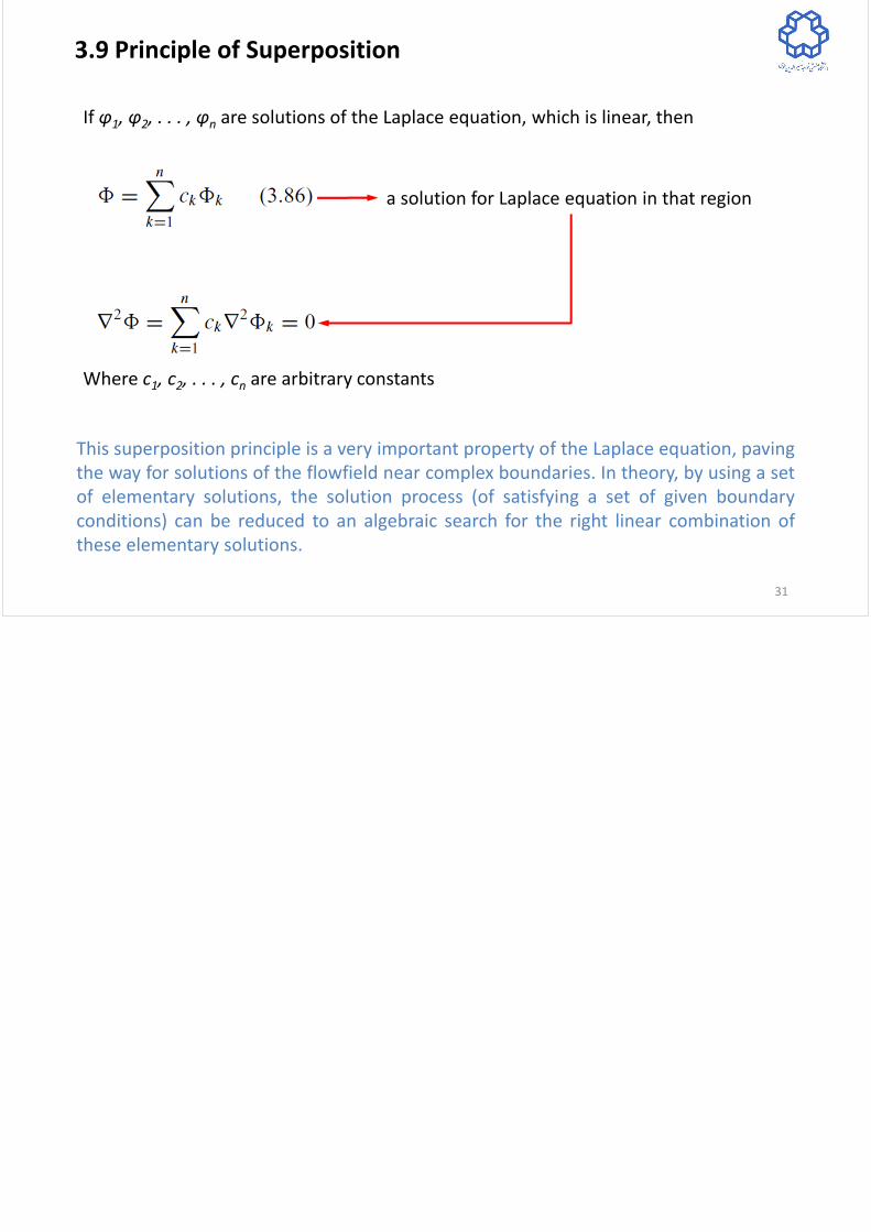
3.9 Principle of Superposition
31
If φ1, φ2, . . . , φn are solutions of the Laplace equation, which is linear, then
a solution for Laplace equation in that region
Where c1, c2, . . . , cn are arbitrary constants
This superposition principle is a very important property of the Laplace equation, paving
the way for solutions of the flowfield near complex boundaries. In theory, by using a set
of elementary solutions, the solution process (of satisfying a set of given boundary
conditions) can be reduced to an algebraic search for the right linear combination of
these elementary solutions.


![Numerical Solution of Incompressible Cahn-Hilliard and ...immiscible, incompressible and density-matched fluids, the basic model so-called Model H [10] has been widely used. It is](https://static.fdocuments.net/doc/165x107/5e5502ff29b40e0f626b1d78/numerical-solution-of-incompressible-cahn-hilliard-and-immiscible-incompressible.jpg)