
General Relativity: An Introduction for Physicists …General Relativity: An Introduction for...
589
General Relativity: An Introduction for Physicists provides a clear mathematical introduction to Einstein’s theory of general relativity. A wide range of applications of the theory are included, with a concentration on its physical consequences. After reviewing the basic concepts, the authors present a clear and intuitive discussion of the mathematical background, including the necessary tools of tensor calculus and differential geometry. These tools are used to develop the topic of special relativity and to discuss electromagnetism in Minkowski spacetime. Gravitation as spacetime curvature is then introduced and the field equations of general relativity are derived. A wide range of applications to physical situations follows, and the conclusion gives a brief discussion of classical field theory and the derivation of general relativity from a variational principle. Written for advanced undergraduate and graduate students, this approachable textbook contains over 300 exercises to illuminate and extend the discussion in the text. Michael Hobson specialised in theoretical physics as an undergraduate at the University of Cambridge and remained at the Cavendish Laboratory to complete a Ph.D. in the physics of star-formation and radiative transfer. As a Research Fellow at Trinity Hall, Cambridge, and later as an Advanced Fellow of the Particle Physics and Astronomy Research Council, he developed an interest in cosmology, in particular in the study of fluctuations in the cosmic microwave background (CMB) radiation. He is currently a Reader in Astrophysics and Cosmology at the Cavendish Laboratory, where he is the principal investigator for the Very Small Array CMB interferometer. He is also joint project scientist for the Arcminute Microkelvin Imager project and an associate of the European Space Agency Planck Surveyor CMB satellite mission. In addition to observational and theo- retical cosmology, his research interests also include Bayesian analysis methods and theoretical optics and he has published over 100 research papers in a wide range of areas. He is a Staff Fellow and Director of Studies in Natural Sciences at Trinity Hall and enjoys an active role in the teaching of undergraduate physics and mathematics. He is a co-author with Ken Riley and Stephen Bence of the well-known undergraduate textbook Mathematical Methods for Physics and Engi- neering (Cambridge, 1998; second edition, 2002; third edition to be published in 2006) and with Ken Riley of the Student’s Solutions Manual accompanying the third edition. George Efstathiou is Professor of Astrophysics and Director of the Institute of Astronomy at the University of Cambridge. After studying physics as an undergraduate at Keble College, Oxford, he gained his Ph.D. in astronomy from Durham University. Following some post-doctoral research at the University of
Transcript of General Relativity: An Introduction for Physicists …General Relativity: An Introduction for...
General Relativity: An Introduction for Physicists provides a clear mathematicalintroduction to Einstein’s theory of general relativity. A wide range of applicationsof the theory are included, with a concentration on its physical consequences.
After reviewing the basic concepts, the authors present a clear and intuitivediscussion of the mathematical background, including the necessary tools of tensorcalculus and differential geometry. These tools are used to develop the topicof special relativity and to discuss electromagnetism in Minkowski spacetime.Gravitation as spacetime curvature is then introduced and the field equations ofgeneral relativity are derived. A wide range of applications to physical situationsfollows, and the conclusion gives a brief discussion of classical field theory andthe derivation of general relativity from a variational principle.
Written for advanced undergraduate and graduate students, this approachabletextbook contains over 300 exercises to illuminate and extend the discussion inthe text.
Michael Hobson specialised in theoretical physics as an undergraduate at theUniversity of Cambridge and remained at the Cavendish Laboratory to completea Ph.D. in the physics of star-formation and radiative transfer. As a ResearchFellow at Trinity Hall, Cambridge, and later as an Advanced Fellow of the ParticlePhysics and Astronomy Research Council, he developed an interest in cosmology,in particular in the study of fluctuations in the cosmic microwave background(CMB) radiation. He is currently a Reader in Astrophysics and Cosmology at theCavendish Laboratory, where he is the principal investigator for the Very SmallArray CMB interferometer. He is also joint project scientist for the ArcminuteMicrokelvin Imager project and an associate of the European Space AgencyPlanck Surveyor CMB satellite mission. In addition to observational and theo-retical cosmology, his research interests also include Bayesian analysis methodsand theoretical optics and he has published over 100 research papers in a widerange of areas. He is a Staff Fellow and Director of Studies in Natural Sciencesat Trinity Hall and enjoys an active role in the teaching of undergraduate physicsand mathematics. He is a co-author with Ken Riley and Stephen Bence of thewell-known undergraduate textbookMathematical Methods for Physics and Engi-neering (Cambridge, 1998; second edition, 2002; third edition to be published in2006) and with Ken Riley of the Student’s Solutions Manual accompanying thethird edition.
George Efstathiou is Professor of Astrophysics and Director of the Instituteof Astronomy at the University of Cambridge. After studying physics as anundergraduate at Keble College, Oxford, he gained his Ph.D. in astronomy fromDurham University. Following some post-doctoral research at the University of
California at Berkeley he returned to work in the UK at the Institute of Astronomy,Cambridge, where he was appointed Assistant Director of Research in 1987.He returned to the Department of Physics at Oxford as Savilian Professor ofAstronomy and Head of Astrophysics, before taking on his current posts at theInstitute of Astronomy in 1997 and 2004 respectively. He is a Fellow of the RoyalSociety and the recipient of several awards, including the Maxwell Medal andPrize of the Institute of Physics in 1990 and the Heineman Prize for Astronomyof the American Astronomical Society in 2005.
Anthony Lasenby is Professor of Astrophysics and Cosmology at the Universityof Cambridge and is currently Head of the Astrophysics Group and the MullardRadio Astronomy Observatory in the Cavendish Laboratory, as well as being aDeputy Head of the Laboratory. He began his astronomical career with a Ph.D.at Jodrell Bank, specializing in the cosmic microwave background, which hasremained a major subject of his research. After a brief period at the National RadioAstronomy Observatory in America, he moved from Manchester to Cambridge in1984 and has been at the Cavendish since then. He is the author or co-author ofover 200 papers spanning a wide range of fields and is the co-author of GeometricAlgebra for Physicists (Cambridge, 2003) with Chris Doran.
General RelativityAn Introduction for Physicists
M . P . HOB SON , G . P . E F S TATH IOUand A . N . LA S ENBY
cambridge university pressCambridge, New York, Melbourne, Madrid, Cape Town, Singapore, São Paulo
Cambridge University PressThe Edinburgh Building, Cambridge cb2 2ru, UK
First published in print format
isbn-13 978-0-521-82951-9
isbn-13 978-0-521-53639-4
isbn-13 978-0-511-13795-2
© M. P. Hobson, G. P. Efstathiou and A. N. Lasenby 2006
2006
Information on this title: www.cambridge.org/9780521829519
This publication is in copyright. Subject to statutory exception and to the provision ofrelevant collective licensing agreements, no reproduction of any part may take placewithout the written permission of Cambridge University Press.
isbn-10 0-511-13795-8
isbn-10 0-521-82951-8
isbn-10 0-521-53639-1
Cambridge University Press has no responsibility for the persistence or accuracy of urlsfor external or third-party internet websites referred to in this publication, and does notguarantee that any content on such websites is, or will remain, accurate or appropriate.
Published in the United States of America by Cambridge University Press, New York
www.cambridge.org
hardback
eBook (Adobe Reader)
eBook (Adobe Reader)
hardback

To our families
Contents
Preface page xv
1 The spacetime of special relativity 11.1 Inertial frames and the principle of relativity 11.2 Newtonian geometry of space and time 31.3 The spacetime geometry of special relativity 31.4 Lorentz transformations as four-dimensional ‘rotations’ 51.5 The interval and the lightcone 61.6 Spacetime diagrams 81.7 Length contraction and time dilation 101.8 Invariant hyperbolae 111.9 The Minkowski spacetime line element 121.10 Particle worldlines and proper time 141.11 The Doppler effect 161.12 Addition of velocities in special relativity 181.13 Acceleration in special relativity 191.14 Event horizons in special relativity 21Appendix 1A: Einstein’s route to special relativity 22Exercises 24
2 Manifolds and coordinates 262.1 The concept of a manifold 262.2 Coordinates 272.3 Curves and surfaces 272.4 Coordinate transformations 282.5 Summation convention 302.6 Geometry of manifolds 312.7 Riemannian geometry 322.8 Intrinsic and extrinsic geometry 33
vii
viii Contents
2.9 Examples of non-Euclidean geometry 362.10 Lengths, areas and volumes 382.11 Local Cartesian coordinates 422.12 Tangent spaces to manifolds 442.13 Pseudo-Riemannian manifolds 452.14 Integration over general submanifolds 472.15 Topology of manifolds 49Exercises 50
3 Vector calculus on manifolds 533.1 Scalar fields on manifolds 533.2 Vector fields on manifolds 543.3 Tangent vector to a curve 553.4 Basis vectors 563.5 Raising and lowering vector indices 593.6 Basis vectors and coordinate transformations 603.7 Coordinate-independent properties of vectors 613.8 Derivatives of basis vectors and the affine connection 623.9 Transformation properties of the affine connection 643.10 Relationship of the connection and the metric 653.11 Local geodesic and Cartesian coordinates 673.12 Covariant derivative of a vector 683.13 Vector operators in component form 703.14 Intrinsic derivative of a vector along a curve 713.15 Parallel transport 733.16 Null curves, non-null curves and affine parameters 753.17 Geodesics 763.18 Stationary property of non-null geodesics 773.19 Lagrangian procedure for geodesics 783.20 Alternative form of the geodesic equations 81Appendix 3A: Vectors as directional derivatives 81Appendix 3B: Polar coordinates in a plane 82Appendix 3C: Calculus of variations 87Exercises 88
4 Tensor calculus on manifolds 924.1 Tensor fields on manifolds 924.2 Components of tensors 934.3 Symmetries of tensors 944.4 The metric tensor 964.5 Raising and lowering tensor indices 97
Contents ix
4.6 Mapping tensors into tensors 974.7 Elementary operations with tensors 984.8 Tensors as geometrical objects 1004.9 Tensors and coordinate transformations 1014.10 Tensor equations 1024.11 The quotient theorem 1034.12 Covariant derivative of a tensor 1044.13 Intrinsic derivative of a tensor along a curve 107Exercises 108
5 Special relativity revisited 1115.1 Minkowski spacetime in Cartesian coordinates 1115.2 Lorentz transformations 1125.3 Cartesian basis vectors 1135.4 Four-vectors and the lightcone 1155.5 Four-vectors and Lorentz transformations 1165.6 Four-velocity 1165.7 Four-momentum of a massive particle 1185.8 Four-momentum of a photon 1195.9 The Doppler effect and relativistic aberration 1205.10 Relativistic mechanics 1225.11 Free particles 1235.12 Relativistic collisions and Compton scattering 1235.13 Accelerating observers 1255.14 Minkowski spacetime in arbitrary coordinates 128Exercises 131
6 Electromagnetism 1356.1 The electromagnetic force on a moving charge 1356.2 The 4-current density 1366.3 The electromagnetic field equations 1386.4 Electromagnetism in the Lorenz gauge 1396.5 Electric and magnetic fields in inertial frames 1416.6 Electromagnetism in arbitrary coordinates 1426.7 Equation of motion for a charged particle 144Exercises 145
7 The equivalence principle and spacetime curvature 1477.1 Newtonian gravity 1477.2 The equivalence principle 1487.3 Gravity as spacetime curvature 1497.4 Local inertial coordinates 151
x Contents
7.5 Observers in a curved spacetime 1527.6 Weak gravitational fields and the Newtonian limit 1537.7 Electromagnetism in a curved spacetime 1557.8 Intrinsic curvature of a manifold 1577.9 The curvature tensor 1587.10 Properties of the curvature tensor 1597.11 The Ricci tensor and curvature scalar 1617.12 Curvature and parallel transport 1637.13 Curvature and geodesic deviation 1657.14 Tidal forces in a curved spacetime 167Appendix 7A: The surface of a sphere 170Exercises 172
8 The gravitational field equations 1768.1 The energy–momentum tensor 1768.2 The energy–momentum tensor of a perfect fluid 1788.3 Conservation of energy and momentum for a perfect fluid 1798.4 The Einstein equations 1818.5 The Einstein equations in empty space 1838.6 The weak-field limit of the Einstein equations 1848.7 The cosmological-constant term 1858.8 Geodesic motion from the Einstein equations 1888.9 Concluding remarks 190Appendix 8A: Alternative relativistic theories of gravity 191Appendix 8B: Sign conventions 193Exercises 193
9 The Schwarzschild geometry 1969.1 The general static isotropic metric 1969.2 Solution of the empty-space field equations 1989.3 Birkhoff’s theorem 2029.4 Gravitational redshift for a fixed emitter and receiver 2029.5 Geodesics in the Schwarzschild geometry 2059.6 Trajectories of massive particles 2079.7 Radial motion of massive particles 2099.8 Circular motion of massive particles 2129.9 Stability of massive particle orbits 2139.10 Trajectories of photons 2179.11 Radial motion of photons 2189.12 Circular motion of photons 2199.13 Stability of photon orbits 220
Contents xi
Appendix 9A: General approach to gravitational redshifts 221Exercises 224
10 Experimental tests of general relativity 23010.1 Precession of planetary orbits 23010.2 The bending of light 23310.3 Radar echoes 23610.4 Accretion discs around compact objects 24010.5 The geodesic precession of gyroscopes 244Exercises 246
11 Schwarzschild black holes 24811.1 The characterisation of coordinates 24811.2 Singularities in the Schwarzschild metric 24911.3 Radial photon worldlines in Schwarzschild coordinates 25111.4 Radial particle worldlines in Schwarzschild coordinates 25211.5 Eddington–Finkelstein coordinates 25411.6 Gravitational collapse and black-hole formation 25911.7 Spherically symmetric collapse of dust 26011.8 Tidal forces near a black hole 26411.9 Kruskal coordinates 26611.10 Wormholes and the Einstein–Rosen bridge 27111.11 The Hawking effect 274Appendix 11A: Compact binary systems 277Appendix 11B: Supermassive black holes 279Appendix 11C: Conformal flatness of two-dimensional Riemannian
manifolds 282Exercises 283
12 Further spherically symmetric geometries 28812.1 The form of the metric for a stellar interior 28812.2 The relativistic equations of stellar structure 29212.3 The Schwarzschild constant-density interior solution 29412.4 Buchdahl’s theorem 29612.5 The metric outside a spherically symmetric
charged mass 29612.6 The Reissner–Nordström geometry: charged
black holes 30012.7 Radial photon trajectories in the RN geometry 30212.8 Radial massive particle trajectories
in the RN geometry 304Exercises 305
xii Contents
13 The Kerr geometry 31013.1 The general stationary axisymmetric metric 31013.2 The dragging of inertial frames 31213.3 Stationary limit surfaces 31413.4 Event horizons 31513.5 The Kerr metric 31713.6 Limits of the Kerr metric 31913.7 The Kerr–Schild form of the metric 32113.8 The structure of a Kerr black hole 32213.9 The Penrose process 32713.10 Geodesics in the equatorial plane 33013.11 Equatorial trajectories of massive particles 33213.12 Equatorial motion of massive particles with
zero angular momentum 33313.13 Equatorial circular motion of massive particles 33513.14 Stability of equatorial massive particle circular orbits 33713.15 Equatorial trajectories of photons 33813.16 Equatorial principal photon geodesics 33913.17 Equatorial circular motion of photons 34113.18 Stability of equatorial photon orbits 34213.19 Eddington–Finkelstein coordinates 34413.20 The slow-rotation limit and gyroscope precession 347Exercises 350
14 The Friedmann–Robertson–Walker geometry 35514.1 The cosmological principle 35514.2 Slicing and threading spacetime 35614.3 Synchronous coordinates 35714.4 Homogeneity and isotropy of the universe 35814.5 The maximally symmetric 3-space 35914.6 The Friedmann–Robertson–Walker metric 36214.7 Geometric properties of the FRW metric 36214.8 Geodesics in the FRW metric 36514.9 The cosmological redshift 36714.10 The Hubble and deceleration parameters 36814.11 Distances in the FRW geometry 37114.12 Volumes and number densities in the FRW geometry 37414.13 The cosmological field equations 37614.14 Equation of motion for the cosmological fluid 37914.15 Multiple-component cosmological fluid 381Exercises 381
Contents xiii
15 Cosmological models 38615.1 Components of the cosmological fluid 38615.2 Cosmological parameters 39015.3 The cosmological field equations 39215.4 General dynamical behaviour of the universe 39315.5 Evolution of the scale factor 39715.6 Analytical cosmological models 40015.7 Look-back time and the age of the universe 40815.8 The distance–redshift relation 41115.9 The volume–redshift relation 41315.10 Evolution of the density parameters 41515.11 Evolution of the spatial curvature 41715.12 The particle horizon, event horizon and Hubble distance 418Exercises 421
16 Inflationary cosmology 42816.1 Definition of inflation 42816.2 Scalar fields and phase transitions in the very early universe 43016.3 A scalar field as a cosmological fluid 43116.4 An inflationary epoch 43316.5 The slow-roll approximation 43416.6 Ending inflation 43516.7 The amount of inflation 43516.8 Starting inflation 43716.9 ‘New’ inflation 43816.10 Chaotic inflation 44016.11 Stochastic inflation 44116.12 Perturbations from inflation 44216.13 Classical evolution of scalar-field perturbations 44216.14 Gauge invariance and curvature perturbations 44616.15 Classical evolution of curvature perturbations 44916.16 Initial conditions and normalisation of curvature perturbations 45216.17 Power spectrum of curvature perturbations 45616.18 Power spectrum of matter-density perturbations 45816.19 Comparison of theory and observation 459Exercises 462
17 Linearised general relativity 46717.1 The weak-field metric 46717.2 The linearised gravitational field equations 47017.3 Linearised gravity in the Lorenz gauge 472
xiv Contents
17.4 General properties of the linearised field equations 47317.5 Solution of the linearised field equations in vacuo 47417.6 General solution of the linearised field equations 47517.7 Multipole expansion of the general solution 48017.8 The compact-source approximation 48117.9 Stationary sources 48317.10 Static sources and the Newtonian limit 48517.11 The energy–momentum of the gravitational field 486Appendix17A:TheEinstein–Maxwell formulationof linearisedgravity 490Exercises 493
18 Gravitational waves 49818.1 Plane gravitational waves and polarisation states 49818.2 Analogy between gravitational and electromagnetic waves 50118.3 Transforming to the transverse-traceless gauge 50218.4 The effect of a gravitational wave on free particles 50418.5 The generation of gravitational waves 50718.6 Energy flow in gravitational waves 51118.7 Energy loss due to gravitational-wave emission 51318.8 Spin-up of binary systems: the binary pulsar PSR B1913+16 51618.9 The detection of gravitational waves 517Exercises 520
19 A variational approach to general relativity 52419.1 Hamilton’s principle in Newtonian mechanics 52419.2 Classical field theory and the action 52719.3 Euler–Lagrange equations 52919.4 Alternative form of the Euler–Lagrange equations 53119.5 Equivalent actions 53319.6 Field theory of a real scalar field 53419.7 Electromagnetism from a variational principle 53619.8 The Einstein–Hilbert action and general relativity in vacuo 53919.9 An equivalent action for general relativity in vacuo 54219.10 The Palatini approach for general relativity in vacuo 54319.11 General relativity in the presence of matter 54519.12 The dynamical energy–momentum tensor 546Exercises 549
Bibliography 555
Index 556
Preface
General relativity is one of the cornerstones of classical physics, providing asynthesis of special relativity and gravitation, and is central to our understandingof many areas of astrophysics and cosmology. This book is intended to give anintroduction to this important subject, suitable for a one-term course for advancedundergraduate or beginning graduate students in physics or in related disciplinessuch as astrophysics and applied mathematics. Some of the later chapters shouldalso provide a useful reference for professionals in the fields of astrophysics andcosmology.
It is assumed that the reader has already been exposed to special relativity andNewtonian gravitation at a level typical of early-stage university physics courses.Nevertheless, a summary of special relativity from first principles is given inChapter 1, and a brief discussion of Newtonian gravity is presented in Chapter 7.No previous experience of 4-vector methods is assumed. Some background inelectromagnetism will prove useful, as will some experience of standard vectorcalculus methods in three-dimensional Euclidean space. The overall level of math-ematical expertise assumed is that of a typical university mathematical methodscourse.
The book begins with a review of the basic concepts underlying special rela-tivity in Chapter 1. The subject is introduced in a way that encourages from theoutset a geometrical and transparently four-dimensional viewpoint, which lays theconceptual foundations for discussion of the more complicated spacetime geome-tries encountered later in general relativity. In Chapters 2–4 we then present amini-course in basic differential geometry, beginning with the introduction ofmanifolds, coordinates and non-Euclidean geometry in Chapter 2. The topic ofvector calculus on manifolds is developed in Chapter 3, and these ideas areextended to general tensors in Chapter 4. These necessary mathematical prelimi-naries are presented in such a way as to make them accessible to physics studentswith a background in standard vector calculus. A reasonable level of mathematical
xv
xvi Preface
rigour has been maintained throughout, albeit accompanied by the occasionalappeal to geometric intuition. The mathematical tools thus developed are thenillustrated in Chapter 5 by re-examining the familiar topic of special relativity in amore formal manner, through the use of tensor calculus in Minkowski spacetime.These methods are further illustrated in Chapter 6, in which electromagnetism isdescribed as a field theory in Minkowski spacetime, serving in some respects as a‘prototype’ for the later discussion of gravitation. In Chapter 7, the incompatibilityof special relativity and Newtonian gravitation is presented and the equivalenceprinciple is introduced. This leads naturally to a discussion of spacetime curvatureand the associated mathematics. The field equations of general relativity are thenderived in Chapter 8, and a discussion of their general properties is presented.
The physical consequences of general relativity in a wide variety of astrophys-ical and cosmological applications are discussed in Chapters 9–18. In particular,the Schwarzschild geometry is derived in Chapter 9 and used to discuss the physicsoutside a massive spherical body. Classic experimental tests of general relativitybased on the exterior Schwarzschild geometry are presented in Chapter 10. Theinterior Schwarzschild geometry and non-rotating black holes are discussed inChapter 11, together with a brief mention of Kruskal coordinates and wormholes.In Chapter 12 we introduce two non-vacuum spherically symmetric geometrieswith a discussion of relativistic stars and charged black holes. Rotating objects arediscussed in Chapter 13, including an extensive discussion of the Kerr solution. InChapters 14–16 we describe the application of general relativity to cosmology andpresent a discussion of the Friedmann–Robertson–Walker geometry, cosmologi-cal models and the theory of inflation, including the generation of perturbationsin the early universe. In Chapter 17 we describe linearised gravitation and weakgravitational fields, in particular drawing analogies with the theory of electromag-netism. The equations of linearised gravitation are then applied to the generation,propagation and detection of weak gravitational waves in Chapter 18. The bookconcludes in Chapter 19 with a brief discussion of classical field theory and thederivation of the field equations of electromagnetism and general relativity fromvariational principles.
Each chapter concludes with a number of exercises that are intended to illumi-nate and extend the discussion in the main text. It is strongly recommended thatthe reader attempt as many of these exercises as time permits, as they should giveample opportunity to test his or her understanding. Occasionally chapters haveappendices containing material that is not central to the development presented inthe main text, but may nevertheless be of interest to the reader. Some appendicesprovide historical context, some discuss current astronomical observations andsome give detailed mathematical derivations that might otherwise interrupt theflow of the main text.
Preface xvii
With regard to the presentation of the mathematics, it has to be acceptedthat equations containing partial and covariant derivatives could be written morecompactly by using the comma and semi-colon notation, e.g. vab for the partialderivative of a vector and vab for its covariant derivative. This would certainlysave typographical space, but many students find the labour of mentally unpackingsuch equations is sufficiently great that it is not possible to think of an equation’sphysical interpretation at the same time. Consequently, we have decided to writeout such expressions in their more obvious but longer form, using bv
a for partialderivatives and bv
a for covariant derivatives.It is worth mentioning that this book is based, in large part, on lecture notes
prepared separately by MPH and GPE for two different relativity courses in theNatural Science Tripos at the University of Cambridge. These courses were firstpresented in this form in the academic year 1999–2000 and are still ongoing. Thecourse presented by MPH consisted of 16 lectures to fourth-year undergraduatesin Part III Physics and Theoretical Physics and covered most of the materialin Chapters 1–11 and 13–14, albeit somewhat rapidly on occasion. The coursegiven by GPE consisted of 24 lectures to third-year undergraduates in Part IIAstrophysics and covered parts of Chapters 1, 5–11, 14 and 18, with an emphasison the less mathematical material. The process of combining the two sets oflecture notes into a homogeneous treatment of relativistic gravitation was aidedsomewhat by the fortuitous choice of a consistent sign convention in the twocourses, and numerous sections have been rewritten in the hope that the readerwill not encounter any jarring changes in presentational style. For many of thetopics covered in the two courses mentioned above, the opportunity has beentaken to include in this book a considerable amount of additional material beyondthat presented in the lectures, especially in the discussion of black holes. Someof this material draws on lecture notes written by ANL for other courses in PartII and Part III Physics and Theoretical Physics. Some topics that were entirelyabsent from any of the above lecture courses have also been included in the book,such as relativistic stars, cosmology, inflation, linearised gravity and variationalprinciples. While every care has been taken to describe these topics in a clear andilluminating fashion, the reader should bear in mind that these chapters have notbeen ‘road-tested’ to the same extent as the rest of the book.
It is with pleasure that we record here our gratitude to those authors fromwhose books we ourselves learnt general relativity and who have certainlyinfluenced our own presentation of the subject. In particular, we acknowledge(in their current latest editions) S. Weinberg, Gravitation and Cosmology,Wiley, 1972; R. M. Wald, General Relativity, University of Chicago Press,1984; B. Schutz, A First Course in General Relativity, Cambridge Univer-sity Press, 1985; W. Rindler, Relativity: Special, General and Cosmological,
xviii Preface
Oxford University Press, 2001; and J. Foster & J. D. Nightingale, A Short Coursein General Relativity, Springer-Verlag, 1995.
During the writing of this book we have received much help and encourage-ment from many of our colleagues at the University of Cambridge, especiallymembers of the Cavendish Astrophysics Group and the Institute of Astronomy.In particular, we thank Chris Doran, Anthony Challinor, Steve Gull and PaulAlexander for numerous useful discussions on all aspects of relativity theory, andDave Green for a great deal of advice concerning typesetting in LaTeX. We arealso especially grateful to Richard Sword for creating many of the diagrams andfigures used in the book and to Michael Bridges for producing the plots of recentmeasurements of the cosmic microwave background and matter power spectra.We also extend our thanks to the Cavendish and Institute of Astronomy teach-ing staff, whose examination questions have provided the basis for some of theexercises included. Finally, we thank several years of undergraduate students fortheir careful reading of sections of the manuscript, for pointing out misprints andfor numerous useful comments. Of course, any errors and ambiguities remainingare entirely the responsibility of the authors, and we would be most grateful tohave them brought to our attention. At Cambridge University Press, we are verygrateful to our editor Vince Higgs for his help and patience and to our copy-editorSusan Parkinson for many useful suggestions that have undoubtedly improved thestyle of the book.
Finally, on a personal note, MPH thanks his wife, Becky, for patiently enduringmany evenings and weekends spent listening to the sound of fingers tapping ona keyboard, and for her unending encouragement. He also thanks his mother,Pat, for her tireless support at every turn. MPH dedicates his contribution to thisbook to the memory of his father, Ron, and to his daughter, Tabitha, whose earlyarrival succeeded in delaying completion of the book by at least three months, butequally made him realise how little that mattered. GPE thanks his wife, Yvonne,for her support. ANL thanks all the students who have sat through his variouslectures on gravitation and cosmology and provided useful feedback. He wouldalso like to thank his family, and particularly his parents, for the encouragementand support they have offered at all times.
1
The spacetime of special relativity
We begin our discussion of the relativistic theory of gravity by reviewing somebasic notions underlying the Newtonian and special-relativistic viewpoints ofspace and time. In order to specify an event uniquely, we must assign it threespatial coordinates and one time coordinate, defined with respect to some frameof reference. For the moment, let us define such a system S by using a set of threemutually orthogonal Cartesian axes, which gives us spatial coordinates x, y andz, and an associated system of synchronised clocks at rest in the system, whichgives us a time coordinate t. The four coordinates t x y z thus label events inspace and time.
1.1 Inertial frames and the principle of relativity
Clearly, one is free to label events not only with respect to a frame S but alsowith respect to any other frame S′, which may be oriented and/or moving withrespect to S in an arbitrary manner. Nevertheless, there exists a class of preferredreference systems called inertial frames, defined as those in which Newton’s firstlaw holds, so that a free particle is at rest or moves with constant velocity, i.e. ina straight line with fixed speed. In Cartesian coordinates this means that
d2x
dt2= d2y
dt2= d2z
dt2= 0
It follows that, in the absence of gravity, if S and S′ are two inertial frames thenS′ can differ from S only by (i) a translation, and/or (ii) a rotation and/or (iii) amotion of one frame with respect to the other at a constant velocity (for otherwiseNewton’s first law would no longer be true). The concept of inertial frames isfundamental to the principle of relativity, which states that the laws of physicstake the same form in every inertial frame. No exception has ever been found to
1
2 The spacetime of special relativity
this general principle, and it applies equally well in both Newtonian theory andspecial relativity.
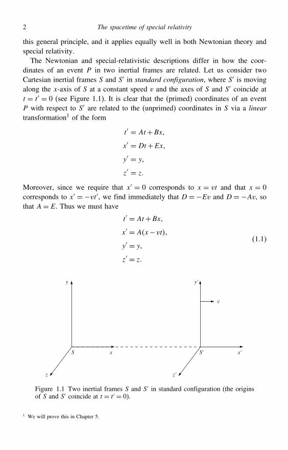
The Newtonian and special-relativistic descriptions differ in how the coor-dinates of an event P in two inertial frames are related. Let us consider twoCartesian inertial frames S and S′ in standard configuration, where S′ is movingalong the x-axis of S at a constant speed v and the axes of S and S′ coincide att = t′ = 0 (see Figure 1.1). It is clear that the (primed) coordinates of an eventP with respect to S′ are related to the (unprimed) coordinates in S via a lineartransformation1 of the form
t′ = At+Bx
x′ = Dt+Ex
y′ = y
z′ = z
Moreover, since we require that x′ = 0 corresponds to x = vt and that x = 0corresponds to x′ = −vt′, we find immediately that D =−Ev and D =−Av, sothat A= E. Thus we must have
t′ = At+Bx
x′ = Ax−vt
y′ = y
z′ = z
(1.1)
x x'
y'y
S S'
z'z
v
Figure 1.1 Two inertial frames S and S′ in standard configuration (the originsof S and S′ coincide at t = t′ = 0).
1 We will prove this in Chapter 5.
1.3 The spacetime geometry of special relativity 3
1.2 Newtonian geometry of space and time
Newtonian theory rests on the assumption that there exists an absolute time, whichis the same for every observer, so that t′ = t. Under this assumption A = 1 andB = 0, and we obtain the Galilean transformation relating the coordinates of anevent P in the two Cartesian inertial frames S and S′:
t′ = t
x′ = x−vt
y′ = y
z′ = z
(1.2)
By symmetry, the expressions for the unprimed coordinates in terms of the primedones have the same form but with v replaced by −v.
The first equation in (1.2) is clearly valid for any two inertial frames S andS′ and shows that the time coordinate of an event P is the same in all inertialframes. The second equation leads to the ‘common sense’ notion of the additionof velocities. If a particle is moving in the x-direction at a speed u in S then itsspeed in S′ is given by
u′x =dx′
dt′= dx′
dt= dx
dt−v= ux−v
Differentiating again shows that the acceleration of a particle is the same in bothS and S′, i.e. du′x/dt′ = dux/dt.
If we consider two events A and B that have coordinates tA xA yA zA
and tB xB yB zB respectively, it is straightforward to show that both the timedifference t = tB− tA and the quantity
r2 = x2+y2+z2
are separately invariant under any Galilean transformation. This leads us toconsider space and time as separate entities. Moreover, the invariance of r2
suggests that it is a geometric property of space itself. Of course, we recogniser2 as the square of the distance between the events in a three-dimensionalEuclidean space. This defines the geometry of space and time in the Newtonianpicture.
1.3 The spacetime geometry of special relativity
In special relativity, Einstein abandoned the postulate of an absolute time andreplaced it by the postulate that the speed of light c is the same in all inertial
4 The spacetime of special relativity
frames.2 By applying this new postulate, together with the principle of relativity,we may obtain the Lorentz transformations connecting the coordinates of an eventP in two different Cartesian inertial frames S and S′.
Let us again consider S and S′ to be in standard configuration (see Figure 1.1),and consider a photon emitted from the (coincident) origins of S and S′ at t =t′ = 0 and travelling in an arbitrary direction. Subsequently the space and timecoordinates of the photon in each frame must satisfy
c2t2−x2−y2− z2 = c2t′2−x′2−y′2− z′2 = 0
Substituting the relations (1.1) into this expression and solving for the constantsA and B, we obtain
ct′ = ct−x
x′ = x−ct
y′ = y
z′ = z
(1.3)
where = v/c and = 1−2−1/2. This Lorentz transformation, also knownas a boost in the x-direction, reduces to the Galilean transformation (1.2) when 1. Once again, symmetry demands that the unprimed coordinates are givenin terms of the primed coordinates by an analogous transformation in which v isreplaced by −v.
From the equations (1.3), we see that the time and space coordinates are ingeneral mixed by a Lorentz transformation (note, in particular, the symmetrybetween ct and x). Moreover, as we shall see shortly, if we consider two eventsA and B with coordinates tA xA yA zA and tB xB yB zB in S, it is straight-forward to show that the interval (squared)
s2 = c2t2−x2−y2−z2 (1.4)
is invariant under any Lorentz transformation. As advocated by Minkowski, theseobservations lead us to consider space and time as united in a four-dimensionalcontinuum called spacetime, whose geometry is characterised by (1.4). We notethat the spacetime of special relativity is non-Euclidean, because of the minussigns in (1.4), and is often called the pseudo-Euclidean or Minkowski geometry.Nevertheless, for any fixed value of t the spatial part of the geometry remainsEuclidean.
2 The reasoning behind Einstein’s proposal is discussed in Appendix 1A.
1.4 Lorentz transformations as four-dimensional ‘rotations’ 5
We have arrived at the familiar viewpoint (to a physicist!) where the physicalworld is modelled as a four-dimensional spacetime continuum that possessesthe Minkowski geometry characterised by (1.4). Indeed, many ideas in specialrelativity are most simply explained by adopting a four-dimensional point of view.
1.4 Lorentz transformations as four-dimensional ‘rotations’
Adopting a particular (Cartesian) inertial frame S corresponds to labelling events inthe Minkowski spacetime with a given set of coordinates t x y z. If we chooseinstead to describe the world with respect to a different Cartesian inertial frameS′ then this corresponds simply to relabelling events in the Minkowski spacetimewith a new set of coordinates t′ x′ y′ z′; the primed and unprimed coordinatesare related by the appropriate Lorentz transformation. Thus, describing physicsin terms of different inertial frames is equivalent to performing a coordinatetransformation on the Minkowski spacetime.
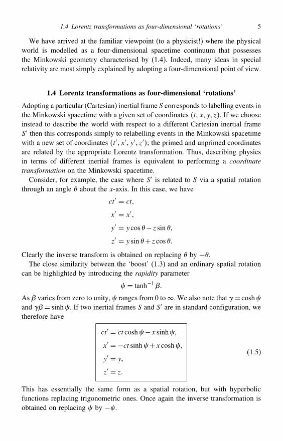
Consider, for example, the case where S′ is related to S via a spatial rotationthrough an angle about the x-axis. In this case, we have
ct′ = ct
x′ = x′
y′ = y cos− z sin
z′ = y sin + z cos
Clearly the inverse transform is obtained on replacing by −.The close similarity between the ‘boost’ (1.3) and an ordinary spatial rotation
can be highlighted by introducing the rapidity parameter
= tanh−1
As varies from zero to unity, ranges from 0 to. We also note that = coshand = sinh. If two inertial frames S and S′ are in standard configuration, wetherefore have
ct′ = ct cosh−x sinh
x′ = −ct sinh+x cosh
y′ = y
z′ = z
(1.5)
This has essentially the same form as a spatial rotation, but with hyperbolicfunctions replacing trigonometric ones. Once again the inverse transformation isobtained on replacing by −.
6 The spacetime of special relativity
x
y
S
z
z'
y'
x'
S'
a
v
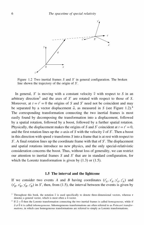
Figure 1.2 Two inertial frames S and S′ in general configuration. The brokenline shown the trajectory of the origin of S′.
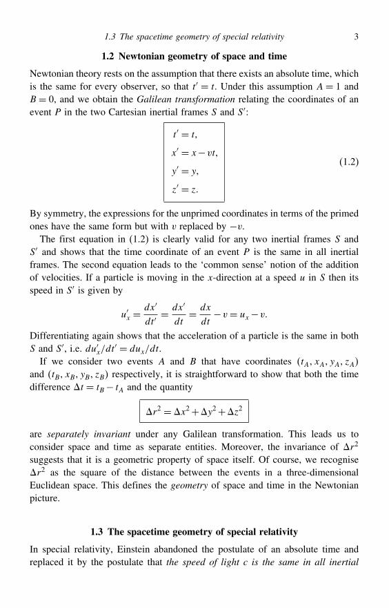
In general, S′ is moving with a constant velocity v with respect to S in anarbitrary direction3 and the axes of S′ are rotated with respect to those of S.Moreover, at t = t′ = 0 the origins of S and S′ need not be coincident and maybe separated by a vector displacement a, as measured in S (see Figure 1.2).4
The corresponding transformation connecting the two inertial frames is mosteasily found by decomposing the transformation into a displacement, followedby a spatial rotation, followed by a boost, followed by a further spatial rotation.Physically, the displacement makes the origins of S and S′ coincident at t= t′ = 0,and the first rotation lines up the x-axis of S with the velocity v of S′. Then a boostin this direction with speed v transforms S into a frame that is at rest with respect toS′. A final rotation lines up the coordinate frame with that of S′. The displacementand spatial rotations introduce no new physics, and the only special-relativisticconsideration concerns the boost. Thus, without loss of generality, we can restrictour attention to inertial frames S and S′ that are in standard configuration, forwhich the Lorentz transformation is given by (1.3) or (1.5).
1.5 The interval and the lightcone
If we consider two events A and B having coordinates t′Ax′A y′A z′A andt′B x′B y′B z′B in S′, then, from (1.5), the interval between the events is given by
3 Throughout this book, the notation v is used specifically to denote three-dimensional vectors, whereas vdenotes a general vector, which is most often a 4-vector.
4 If a= 0 then the Lorentz transformation connecting the two inertial frames is called homogeneous, while ifa = 0 it is called inhomogeneous. Inhomogeneous transformations are often referred to as Poincaré transfor-mations, in which case homogeneous transformations are referred to simply as Lorentz transformations.
1.5 The interval and the lightcone 7
s2 = c2t′2−x′2−y′2−z′2
= ct cosh− x sinh2− −ct sinh+ x cosh2
−y2−z2
= c2t2−x2−y2−z2
Thus the interval is invariant under the boost (1.5) and, from the above discussion,we may infer that s2 is in fact invariant under any Poincaré transformation. Thissuggests that the interval is an underlying geometrical property of the spacetimeitself, i.e. an invariant ‘distance’ between events in spacetime. It also follows thatthe sign of s2 is defined invariantly, as follows:
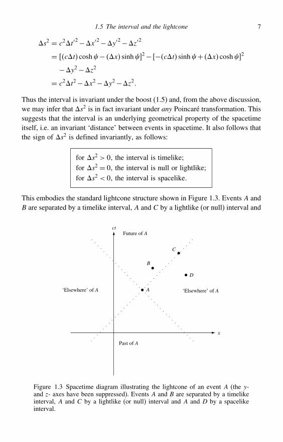
for s2 > 0 the interval is timelikefor s2 = 0 the interval is null or lightlikefor s2 < 0 the interval is spacelike
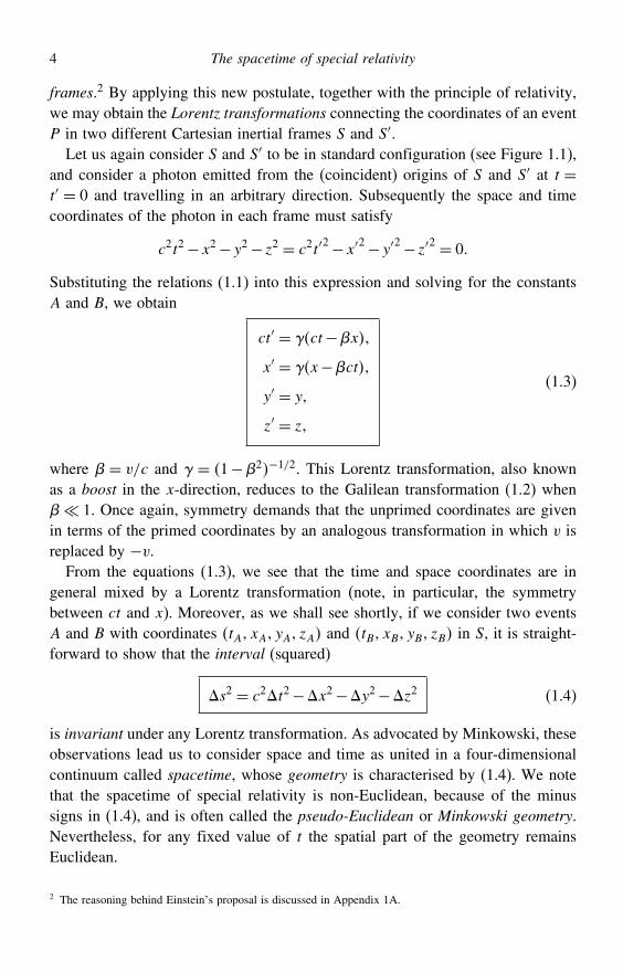
This embodies the standard lightcone structure shown in Figure 1.3. Events A andB are separated by a timelike interval, A and C by a lightlike (or null) interval and
ct
x
A
Future of A
Past of A
D
‘Elsewhere’ of A ‘Elsewhere’ of A
C
B
Figure 1.3 Spacetime diagram illustrating the lightcone of an event A (the y-and z- axes have been suppressed). Events A and B are separated by a timelikeinterval, A and C by a lightlike (or null) interval and A and D by a spacelikeinterval.
8 The spacetime of special relativity
A and D by a spacelike interval. The geometrical distinction between timelike andspacelike intervals corresponds to a physical distinction: if the interval is timelikethen we can find an inertial frame in which the events occur at the same spatialcoordinates and if the interval is spacelike then we can find an inertial framein which the events occur at the same time coordinate. This becomes obviouswhen we consider the spacetime diagram of a Lorentz transformation; we shalldo this next.
1.6 Spacetime diagrams
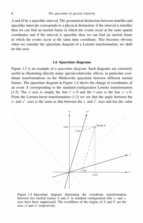
Figure 1.3 is an example of a spacetime diagram. Such diagrams are extremelyuseful in illustrating directly many special-relativistic effects, in particular coor-dinate transformations on the Minkowski spacetime between different inertialframes. The spacetime diagram in Figure 1.4 shows the change of coordinates ofan event A corresponding to the standard-configuration Lorentz transformation(1.5). The x′-axis is simply the line t′ = 0 and the t′-axis is the line x′ = 0.From the Lorentz-boost transformation (1.3) we see that the angle between thex- and x′- axes is the same as that between the t- and t′- axes and has the value
t (A)
ct ct'
x
x'
t' (A)
x' (A)
Event A
x (A)
Figure 1.4 Spacetime diagram illustrating the coordinate transformationbetween two inertial frames S and S′ in standard configuration (the y- and z-axes have been suppressed). The worldlines of the origins of S and S′ are theaxes ct and ct′ respectively.
1.6 Spacetime diagrams 9
tan−1v/c. Moreover, we note that the t- and t′- axes are also the worldlines ofthe origins of S and S′ respectively.
It is important to realise that the coordinates of the event A in the frame S′ arenot obtained by extending perpendiculars from A to the x′- and t′- axes. Sincethe x′-axis is simply the line t′ = 0, it follows that lines of simultaneity in S′ areparallel to the x′-axis. Similarly, lines of constant x′ are parallel to the t′-axis. Thesame reasoning is equally valid for obtaining the coordinates of A in the frameS but, since the x- and t- axes are drawn as orthogonal in the diagram, this isequivalent simply to extending perpendiculars from A to the x- and t- axes in themore familiar manner.
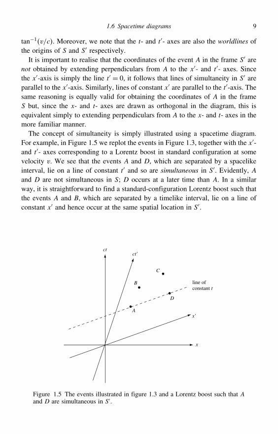
The concept of simultaneity is simply illustrated using a spacetime diagram.For example, in Figure 1.5 we replot the events in Figure 1.3, together with the x′-and t′- axes corresponding to a Lorentz boost in standard configuration at somevelocity v. We see that the events A and D, which are separated by a spacelikeinterval, lie on a line of constant t′ and so are simultaneous in S′. Evidently, Aand D are not simultaneous in S; D occurs at a later time than A. In a similarway, it is straightforward to find a standard-configuration Lorentz boost such thatthe events A and B, which are separated by a timelike interval, lie on a line ofconstant x′ and hence occur at the same spatial location in S′.
line ofconstant t'
x'
ct'ct
x
A
D
C
B
Figure 1.5 The events illustrated in figure 1.3 and a Lorentz boost such that Aand D are simultaneous in S′.
10 The spacetime of special relativity
1.7 Length contraction and time dilation
Two elementary (but profound) consequences of the Lorentz transformationsare length contraction and time dilation. Both these effects are easily derivedfrom (1.3).
Length contraction
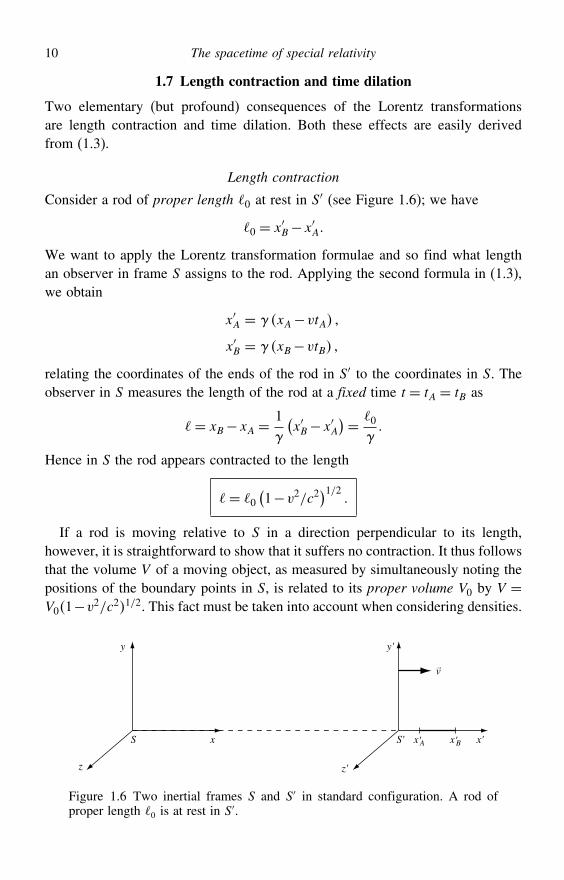
Consider a rod of proper length 0 at rest in S′ (see Figure 1.6); we have
0 = x′B−x′A
We want to apply the Lorentz transformation formulae and so find what lengthan observer in frame S assigns to the rod. Applying the second formula in (1.3),we obtain
x′A = xA−vtA
x′B = xB−vtB
relating the coordinates of the ends of the rod in S′ to the coordinates in S. Theobserver in S measures the length of the rod at a fixed time t = tA = tB as
= xB−xA =1
(x′B−x′A
)= 0
Hence in S the rod appears contracted to the length
= 0(1−v2/c2
)1/2
If a rod is moving relative to S in a direction perpendicular to its length,however, it is straightforward to show that it suffers no contraction. It thus followsthat the volume V of a moving object, as measured by simultaneously noting thepositions of the boundary points in S, is related to its proper volume V0 by V =V01−v2/c21/2. This fact must be taken into account when considering densities.
x x'
y'y
S S'
z'z
v
x A' x B'
Figure 1.6 Two inertial frames S and S′ in standard configuration. A rod ofproper length 0 is at rest in S′.
1.8 Invariant hyperbolae 11
‘Click 1’ ‘Click 2’
x'A x'Ax'
y'
S'
z'
x'
y'
S'
z'
x
y
S
z
vv
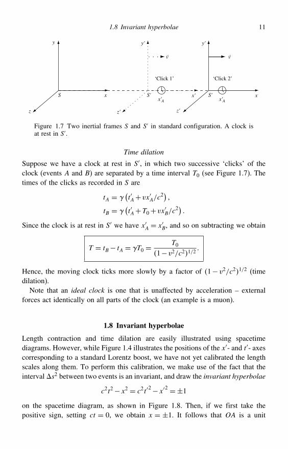
Figure 1.7 Two inertial frames S and S′ in standard configuration. A clock isat rest in S′.
Time dilation
Suppose we have a clock at rest in S′, in which two successive ‘clicks’ of theclock (events A and B) are separated by a time interval T0 (see Figure 1.7). Thetimes of the clicks as recorded in S are
tA = (t′A+vx′A/c
2) tB =
(t′A+T0+vx′B/c
2) Since the clock is at rest in S′ we have x′A = x′B, and so on subtracting we obtain
T = tB− tA = T0 =T0
1−v2/c21/2
Hence, the moving clock ticks more slowly by a factor of 1− v2/c21/2 (timedilation).
Note that an ideal clock is one that is unaffected by acceleration – externalforces act identically on all parts of the clock (an example is a muon).
1.8 Invariant hyperbolae
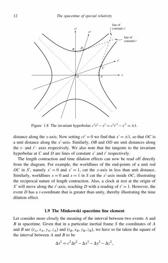
Length contraction and time dilation are easily illustrated using spacetimediagrams. However, while Figure 1.4 illustrates the positions of the x′- and t′- axescorresponding to a standard Lorentz boost, we have not yet calibrated the lengthscales along them. To perform this calibration, we make use of the fact that theinterval s2 between two events is an invariant, and draw the invariant hyperbolae
c2t2−x2 = c2t′2−x′2 =±1on the spacetime diagram, as shown in Figure 1.8. Then, if we first take thepositive sign, setting ct = 0, we obtain x = ±1. It follows that OA is a unit
12 The spacetime of special relativity
x'
ct'
O
line ofconstant x'
line ofconstant t'
C
D
ct
xA
B
Figure 1.8 The invariant hyperbolae c2t2−x2 = c2t′2−x′2 =±1.
distance along the x-axis. Now setting ct′ = 0 we find that x′ = ±1, so that OC isa unit distance along the x′-axis. Similarly, OB and OD are unit distances alongthe t- and t′- axes respectively. We also note that the tangents to the invarianthyperbolae at C and D are lines of constant x′ and t′ respectively.The length contraction and time dilation effects can now be read off directly
from the diagram. For example, the worldlines of the end-points of a unit rodOC in S′, namely x′ = 0 and x′ = 1, cut the x-axis in less than unit distance.Similarly, worldlines x = 0 and x = 1 in S cut the x′-axis inside OC, illustratingthe reciprocal nature of length contraction. Also, a clock at rest at the origin ofS′ will move along the t′-axis, reaching D with a reading of t′ = 1. However, theevent D has a t-coordinate that is greater than unity, thereby illustrating the timedilation effect.
1.9 The Minkowski spacetime line element
Let consider more closely the meaning of the interval between two events A andB in spacetime. Given that in a particular inertial frame S the coordinates of Aand B are tA xA yA zA and tB xB yB zB, we have so far taken the square ofthe interval between A and B to be
s2 = c2t2−x2−y2−z2
1.9 The Minkowski spacetime line element 13
ct
x
B
A
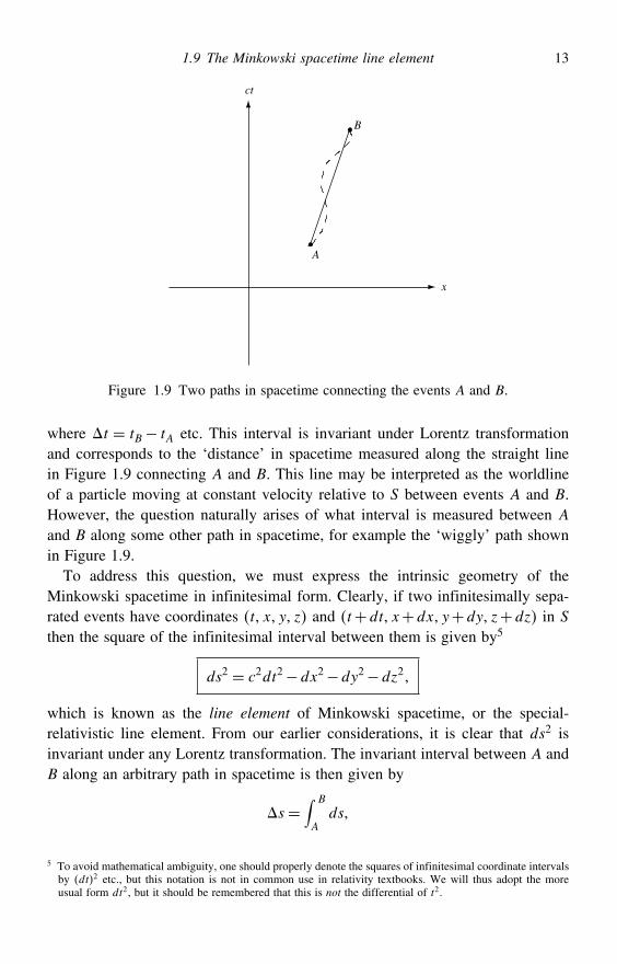
Figure 1.9 Two paths in spacetime connecting the events A and B.
where t = tB− tA etc. This interval is invariant under Lorentz transformationand corresponds to the ‘distance’ in spacetime measured along the straight linein Figure 1.9 connecting A and B. This line may be interpreted as the worldlineof a particle moving at constant velocity relative to S between events A and B.However, the question naturally arises of what interval is measured between A
and B along some other path in spacetime, for example the ‘wiggly’ path shownin Figure 1.9.
To address this question, we must express the intrinsic geometry of theMinkowski spacetime in infinitesimal form. Clearly, if two infinitesimally sepa-rated events have coordinates t x y z and t+dt x+dx y+dy z+dz in S
then the square of the infinitesimal interval between them is given by5
ds2 = c2dt2−dx2−dy2−dz2
which is known as the line element of Minkowski spacetime, or the special-relativistic line element. From our earlier considerations, it is clear that ds2 isinvariant under any Lorentz transformation. The invariant interval between A andB along an arbitrary path in spacetime is then given by
s =∫ B
Ads
5 To avoid mathematical ambiguity, one should properly denote the squares of infinitesimal coordinate intervalsby dt2 etc., but this notation is not in common use in relativity textbooks. We will thus adopt the moreusual form dt2, but it should be remembered that this is not the differential of t2.
14 The spacetime of special relativity
where the integral is evaluated along the particular path under consideration.Clearly, to perform this integral we must have a set of equations describing thespacetime path.
1.10 Particle worldlines and proper time
Let us now turn to the description of the motion of a particle in spacetime terms.A particle describes a worldline in spacetime. In general, for two infinitesimallyseparated events in spacetime; by analogy with our earlier discussion we have:
for ds2 > 0 the interval is timelike
for ds2 = 0 the interval is null or lightlike
for ds2 < 0 the interval is spacelike
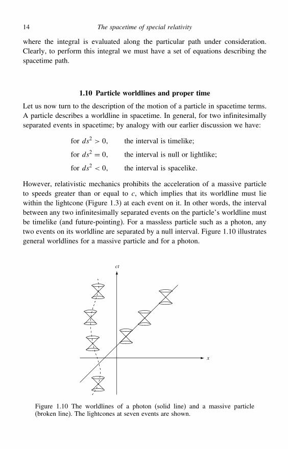
However, relativistic mechanics prohibits the acceleration of a massive particleto speeds greater than or equal to c, which implies that its worldline must liewithin the lightcone (Figure 1.3) at each event on it. In other words, the intervalbetween any two infinitesimally separated events on the particle’s worldline mustbe timelike (and future-pointing). For a massless particle such as a photon, anytwo events on its worldline are separated by a null interval. Figure 1.10 illustratesgeneral worldlines for a massive particle and for a photon.
ct
x
Figure 1.10 The worldlines of a photon (solid line) and a massive particle(broken line). The lightcones at seven events are shown.
1.10 Particle worldlines and proper time 15
A particle worldline may be described by giving x, y and z as functions of tin some inertial frame S. However, a more four-dimensional way of describing aworldline is to give the four coordinates t x y z of the particle in S as functionsof a parameter that varies monotonically along the worldline. Given the fourfunctions t, x, y and z, each value of determines a point alongthe curve. Any such parameter is possible, but a natural one to use for a massiveparticle is its proper time.
We define the proper time interval d between two infinitesimally separatedevents on the particle’s worldline by
c2d2 = ds2 (1.6)
Thus, if the coordinate differences in S between the two events are dtdxdydzthen we have
c2d2 = c2dt2−dx2−dy2−dz2
Hence the proper time interval between the events is given by
d = 1−v2/c21/2dt = dt/v
where v is the speed of the particle with respect to S over this infinitesimalinterval. If we integrate d between two points A and B on the worldline, weobtain the total elapsed proper time interval:
=∫ B
Ad =
∫ B
A
[1− v2t
c2
]1/2dt (1.7)
We see that if the particle is at rest in S then the proper time is just thecoordinate time t measured by clocks at rest in S. If at any instant in the historyof the particle we introduce an instantaneous rest frame S′ such that the particleis momentarily at rest in S′ then we see that the proper time is simply thetime recorded by a clock that moves along with the particle. It is therefore aninvariantly defined quantity, a fact that is clear from (1.6).
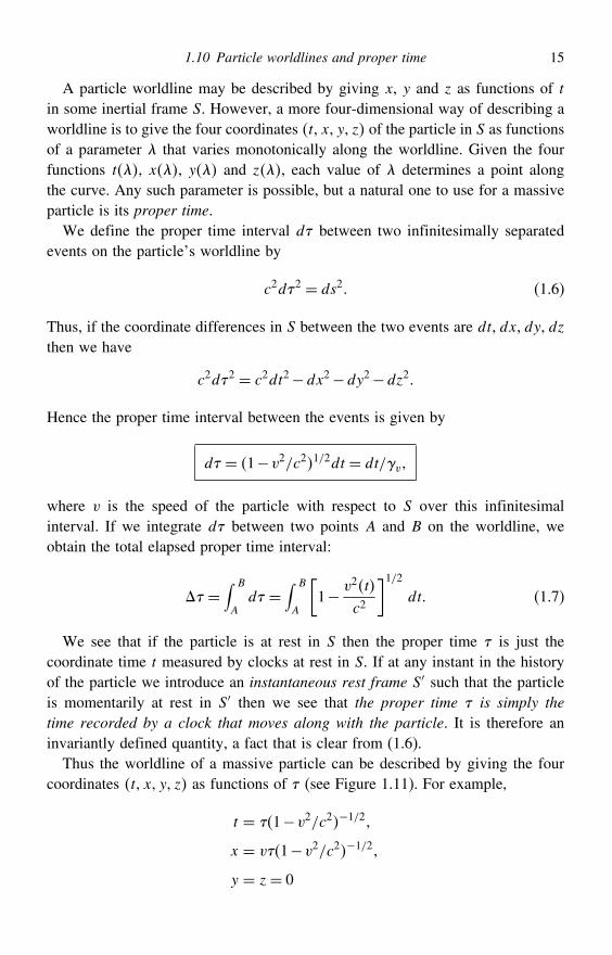
Thus the worldline of a massive particle can be described by giving the fourcoordinates t x y z as functions of (see Figure 1.11). For example,
t = 1−v2/c2−1/2
x = v1−v2/c2−1/2
y = z= 0
16 The spacetime of special relativity
τ
τ = –2
τ = –1
τ = 0
τ = 1
τ = 2
τ = 3
ct
x
Figure 1.11 A path in the t x-plane can be specified by giving one coordinatein terms of the other, for example x = xt, or alternatively by giving bothcoordinates as functions of a parameter along the curve: t = t x = x.For massive particles the natural parameter to use is the proper time .
is the worldline of a particle, moving at constant speed v along the x-axis of S,which passes through the origin of S at t = 0.
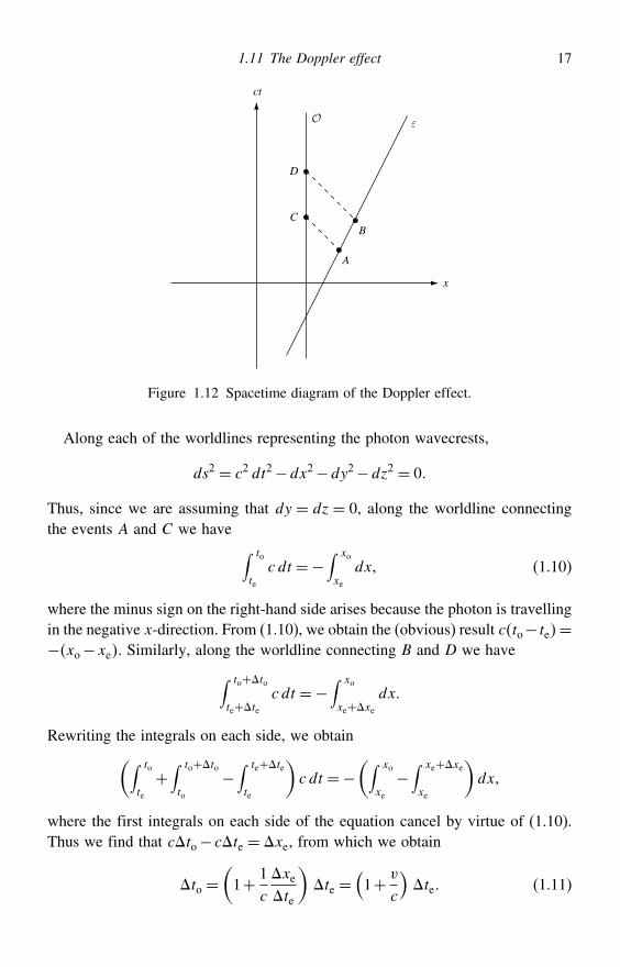
1.11 The Doppler effect
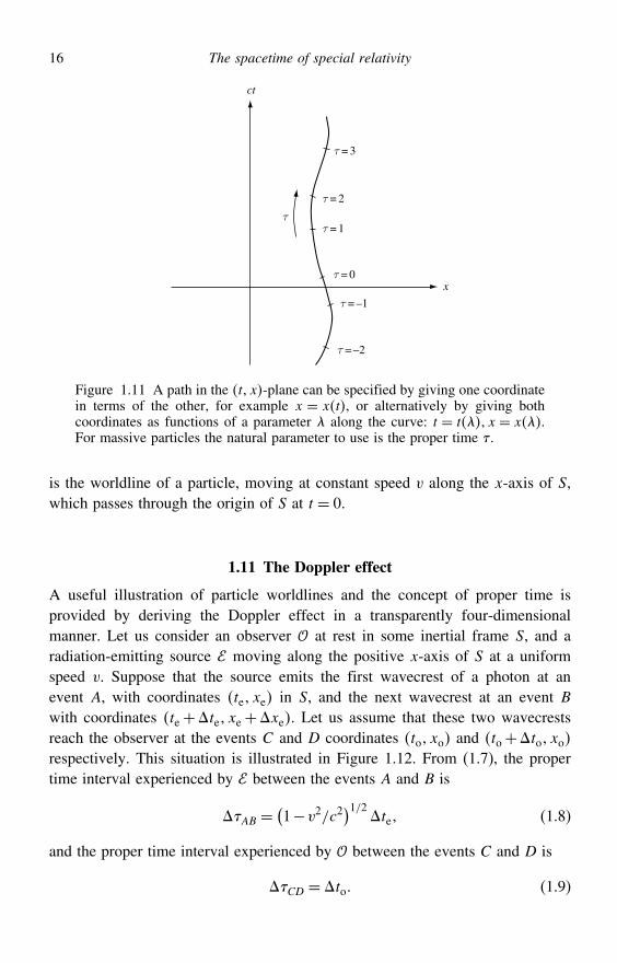
A useful illustration of particle worldlines and the concept of proper time isprovided by deriving the Doppler effect in a transparently four-dimensionalmanner. Let us consider an observer at rest in some inertial frame S, and aradiation-emitting source moving along the positive x-axis of S at a uniformspeed v. Suppose that the source emits the first wavecrest of a photon at anevent A, with coordinates te xe in S, and the next wavecrest at an event Bwith coordinates te+te xe+xe. Let us assume that these two wavecrestsreach the observer at the events C and D coordinates to xo and to+to xo
respectively. This situation is illustrated in Figure 1.12. From (1.7), the propertime interval experienced by between the events A and B is
AB =(1−v2/c2
)1/2te (1.8)
and the proper time interval experienced by between the events C and D is
CD = to (1.9)
1.11 The Doppler effect 17
ε
D
CB
A
ct
x
Figure 1.12 Spacetime diagram of the Doppler effect.
Along each of the worldlines representing the photon wavecrests,
ds2 = c2 dt2−dx2−dy2−dz2 = 0
Thus, since we are assuming that dy = dz = 0, along the worldline connectingthe events A and C we have ∫ to
te
c dt =−∫ xo
xe
dx (1.10)
where the minus sign on the right-hand side arises because the photon is travellingin the negative x-direction. From (1.10), we obtain the (obvious) result cto−te=−xo−xe. Similarly, along the worldline connecting B and D we have∫ to+to
te+tec dt =−
∫ xo
xe+xedx
Rewriting the integrals on each side, we obtain(∫ to
te
+∫ to+toto
−∫ te+tete
)c dt =−
(∫ xo
xe
−∫ xe+xexe
)dx
where the first integrals on each side of the equation cancel by virtue of (1.10).Thus we find that cto− cte = xe, from which we obtain
to =(1+ 1
c
xete
)te =
(1+ v
c
)te (1.11)
18 The spacetime of special relativity
Hence, using (1.8), (1.9) and (1.11), we can derive the ratio of the proper timeintervals CD and AB experienced by and respectively:
CDAB
= 1+te1−21/2te
= 1+
1−1/21+1/2= 1+1/2
1−1/2
This ratio must be the reciprocal of the ratio of the photon’s frequency as measuredby and respectively, and thus we obtain the familiar Doppler-effect formula
=(1−
1+
)1/2
(1.12)
1.12 Addition of velocities in special relativity
If a particle’s worldline is described by giving x, y and z as functions of t insome inertial frame S then the components of its velocity in S at any point are
ux =dx
dt uy =
dy
dt uz =
dz
dt
The components of its velocity in some other inertial frame S′ are usually obtainedby taking differentials of the Lorentz transformation. For inertial frames S and S′related by a boost v in standard configuration, we have from (1.3)
dt′ = vdt−vdx/c2 dx′ = vdx−vdt dy′ = dy dz′ = dz
where we have made explicit the dependence of on v. We immediately obtain
u′x =dx′
dt′= ux−v
1−uxv/c2
u′y =dy′
dt′= uy
v1−uxv/c2
u′z =dz′
dt′= uz
v1−uxv/c2
(1.13)
These replace the ‘common sense’ addition-of-velocities formulae of Newtonianmechanics. The inverse transformations are obtained by replacing v by −v.
The special-relativistic addition of velocities along the same direction iselegantly expressed using the rapidity parameter (Section 1.4). For example,consider three inertial frames S, S′ and S′′. Suppose that S′ is related to S by aboost of speed v in the x-direction and that S′′ is related to S′ by a boost of speedu′ in the x′-direction. Using (1.5), we quickly find that
ct′′ = ct coshv+u′−x sinhv+u′
1.13 Acceleration in special relativity 19
x′′ = −ct sinhv+u′+x coshv+u′
y′′ = y
z′′ = z
where tanhv = v/c and tanhu′ = u′/c. This shows that S′′ is connected to S
by a boost in the x-direction with speed u, where u/c = tanhv+u′. Thus wesimply add the rapidities (in a similar way to adding the angles of two spatialrotations about the same axis). This gives
u= c tanhv+u′= ctanhv+ tanhu′
1+ tanhv tanhu′= u′ +v
1+u′v/c2
which is the special-relativistic formula for the addition of velocities in the samedirection.
1.13 Acceleration in special relativity
The components of the acceleration of a particle in S are defined as
ax =duxdt
ay =duy
dt az =
duzdt
and the corresponding quantities in S′ are obtained from the differential forms ofthe expressions (1.13). For example,
du′x =dux
2v 1−uxv/c
22
Also, from the Lorentz transformation (1.3) we find that
dt′ = vdt−vdx/c2= v1−uxv/c2dt
So, for example, we have
a′x =du′xdt′
= 13v 1−uxv/c
23ax (1.14)
Similarly, we obtain
a′y =du′ydt′
= 12v 1−uxv/c
22ay+
uyv
c22v 1−uxv/c
23ax
a′z =du′zdt′
= 12v 1−uxv/c
22az+
uzv
c22v 1−uxv/c
23ax
20 The spacetime of special relativity
We see from these transformation formulae that acceleration is not invariantin special relativity, unlike in Newtonian mechanics, as discussed in Section 1.2.However, it is clear that acceleration is an absolute quantity, that is, all observersagree upon whether a body is accelerating. If the acceleration is zero in oneinertial frame, it is necessarily zero in any other frame.
Let us investigate the worldline of an accelerated particle. To make our illus-tration concrete, we consider a spaceship moving at a variable speed ut relativeto some inertial frame S and suppose that an observer B in the spaceship makesa continuous record of his accelerometer reading f as a function of his ownproper time .
We begin by introducing an instantaneous rest frame (IRF) S′, which, at eachinstant, is an inertial frame moving at the same speed v as the spaceship, i.e. v= u.Thus, at any instant, the velocity of the spaceship in the IRF S′ is zero, i.e. u′ = 0.Moreover, from the above discussion of proper time, it should be clear that at anyinstant an interval of proper time is equal to an interval of coordinate time in theIRF, i.e. = t′. An accelerometer measures the rate of change of velocity, sothat, during a small interval of proper time , B will record that his velocity haschanged by an amount f. Therefore, at any instant, in the IRF S′ we have
du′
dt′= du′
d= f
From (1.14), we thus obtain
du
dt=(1− u2
c2
)3/2
f
However, since d = 1−u2/c21/2 dt, we find that
du
d=(1− u2
c2
)f
which integrates easily to give
u= c tanh
where c= ∫ 0 f ′d ′ and we have taken u = 0 to be zero. Thus we have
an expression for the velocity of the spaceship in S as a function of B’s proper time.To parameterise the worldline of the spaceship in S, we note that
dt
d=(1− u2
c2
)−1/2= cosh
dx
d= u
(1− u2
c2
)−1/2= c sinh (1.15)
Integration of these equations with respect to gives the functions t and x.
1.14 Event horizons in special relativity 21
1.14 Event horizons in special relativity
The presence of acceleration can produce surprising effects. Consider for simplic-ity the case of uniform acceleration. By this we mean we do not mean thatdu/dt = constant, since this is inappropiate in special relativity because it wouldimply that u→ as t→, which is not permitted. Instead, uniform acceler-ation in special relativity means that the accelerometer reading f is constant.A spaceship whose engine is set at a constant emission rate would be uniformlyaccelerated in this sense.
Thus, if f = constant, we have = f/c. The equations (1.15) are then easilyintegrated to give
t = t0+c
fsinh
f
c
x = x0+c2
f
(cosh
f
c−1
)
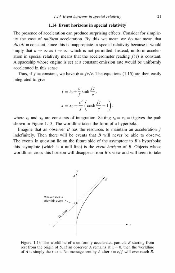
where t0 and x0 are constants of integration. Setting t0 = x0 = 0 gives the pathshown in Figure 1.13. The worldline takes the form of a hyperbola.
Imagine that an observer B has the resources to maintain an acceleration f
indefinitely. Then there will be events that B will never be able to observe.The events in question lie on the future side of the asymptote to B’s hyperbola;this asymplote (which is a null line) is the event horizon of B. Objects whoseworldlines cross this horizon will disappear from B’s view and will seem to take
Horizo
n
B never sees Aafter this event
ct
x
BA
Figure 1.13 The worldline of a uniformly accelerated particle B starting fromrest from the origin of S. If an observer A remains at x = 0, then the worldlineof A is simply the t-axis. No message sent by A after t = c/f will ever reach B.
22 The spacetime of special relativity
for ever to do so. Nevertheless, the objects themselves cross the horizon in a finiteproper time and still have an infinite lifetime ahead of them.
Appendix 1A: Einstein’s route to special relativity
Most books on special relativity begin with some sort of description of theMichelson–Morley experiment and then introduce the Lorentz transformation. Infact, Einstein claimed that he was not influenced by this experiment. This isdisputed by various historians of science and biographers of Einstein. One mightthink that these scholars are on strong ground, especially given that the experimentis referred to (albeit obliquely) in Einstein’s papers. However, it may be worthtaking Einstein’s claim at face value.
Remember that Einstein was a theorist – one of the greatest theorists who hasever lived – and he had a theorist’s way of looking at physics. A good theoristdevelops an intuition about how Nature works, which helps in the formulationof physical laws. For example, possible symmetries and conserved quantities areconsidered. We can get a strong clue about Einstein’s thinking from the title ofhis famous 1905 paper on special relativity. The first paragraph is reproducedbelow.
On the Electrodynamics of Moving Bodiesby A. Einstein
It is known that Maxwell’s electrodynamics – as usually understood at the present time –when applied to moving bodies, leads to asymmetries which do not appear to be inherentin the phenomena. Take, for example, the reciprocal electrodynamic action of a magnetand a conductor. The observable phenomenon here depends only on the relative motionof the conductor and the magnet, whereas the customary view draws a sharp distinctionbetween the two cases in which either the one or the other of these bodies is in motion.For if the magnet is in motion and the conductor at rest, there arises in the neighbourhoodof the magnet an electric field with a certain definite energy, producing a current at theplaces where parts of the conductor are situated. But if the magnet is stationary andthe conductor in motion, no electric field arises in the neighbourhood of the magnet. Inthe conductor, however, we find an electromotive force, to which in itself there is nocorresponding energy, but which gives rise – assuming equality of relative motion in thetwo cases discussed – to electric currents of the same path and intensity as those producedby the electric forces in the former case.
You see that Einstein’s paper is not called ‘Transformations between inertialframes’, or ‘A theory in which the speed of light is assumed to be a universalconstant’. Electrodynamics is at the heart of Einstein’s thinking; Einstein realizedthat Maxwell’s equations of electromagnetism required special relativity.
Appendix 1A: Einstein’s route to special relativity 23
Maxwell’s equations are
· D = · B = 0
× E =−Bt
× H = j+ Dt
where D= 0 E+ P and B= 0 H+ M, P and M being respectively the polari-sation and the magnetisation of the medium in which the fields are present. In freespace we can set j= 0 and = 0, and we then get the more obviously symmetricalequations
· E = 0 · B = 0
× E =−Bt
× B = 00 Et
Taking the curl of the equation for × E, applying the relation
× × E= · E−2 Eand performing a similar operation for B in the equation for × B, we derive theequations for electromagnetic waves:
2 E = 002 Et2
2 B = 002 Bt2
These both have the form of a wave equation with a propagation speed c =1/√00. Now, the constants 0 and 0 are properties of the ‘vacuum’:
0 the permeability of a vacuum, equals 4×10⁻⁷ Hm−1
0 the permittivity of a vacuum, equals 885×10−12 Fm−1
This relation between the constants 0 and 0 and the speed of light was one ofthe most startling consequences of Maxwell’s theory. But what do we mean by a‘vacuum’? Does it define an absolute frame of rest? If we deny the existence of anabsolute frame of rest then how do we formulate a theory of electromagnetism?How do Maxwell’s equations appear in frames moving with respect to each other?Do we need to change the value of c? If we do, what will happen to the valuesof 0 and 0?
Einstein solves all of these problems at a stroke by saying that Maxwell’sequations take the same mathematical form in all inertial frames. The speed of lightc is thus the same in all inertial frames. The theory of special relativity (includingamazing conclusions such as E = mc2) follows from a generalisation of thissimple and theoretically compelling assumption. Maxwell’s equations thereforerequire special relativity. You see that for a master theorist like Einstein, the
24 The spacetime of special relativity
Michelson–Morley experiment might well have been a side issue. Einstein could‘see’ special relativity lurking in Maxwell’s equations.
Exercises
1.1 For two inertial frames S and S′ in standard configuration, show that the coordinatesof any given event in each frame are related by the Lorentz tranformations (1.3).
1.2 Two events A and B have coordinates tA xA yA zA and tB xB yB zB respectively.Show that both the time difference t = tB− tA and the quantity
r2 = x2+y2+z2
are separately invariant under any Galilean transformation, whereas the quantity
s2 = c2t2−x2−y2−z2
is invariant under any Lorentz transformation.1.3 In a given inertial frame two particles are shot out simultaneously from a given
point, with equal speeds v in orthogonal directions. What is the speed of each particlerelative to the other?
1.4 An inertial frame S′ is related to S by a boost of speed v in the x-direction, and S′′
is related to S′ by a boost of speed u′ in the x′-direction. Show that S′′ is related toS by a boost in the x-direction with speed u, where
u= c tanhv+u′
tanhv = v/c and tanhu′ = u′/c.1.5 An inertial frame S′ is related to S by a boost v whose components in S are vx vy vz.
Show that the coordinates ct′ x′ y′ z′ and ct x y z of an event are related by⎛⎜⎜⎜⎝ct′
x′
y′
z′
⎞⎟⎟⎟⎠=⎛⎜⎜⎜⎝
−x −y −z
−x 1+2x xy xz
−y yx 1+2y yz
−y zx zy 1+2z
⎞⎟⎟⎟⎠⎛⎜⎜⎜⎝ct
x
y
z
⎞⎟⎟⎟⎠
where = v/c = 1−2−1/2 and = − 1/2. Hint: The transformationmust take the same form if both S and S′ undergo the same spatial rotation.
1.6 An inertial frame S′ is related to S by a boost of speed u in the positive x-direction.Similarly, S′′ is related to S′ by a boost of speed v in the y′-direction. Find thetransformation relating the coordinates ct x y z and ct′′ x′′ y′′ z′′ and hencedescribe how S and S′′ are physically related.
1.7 The frames S and S′ are in standard configuration. A straight rod rotates at a uniformangular velocity ′ about its centre, which is fixed at the origin of S′. If the rod liesalong the x′-axis at t′ = 0, obtain an equation for the shape of the rod in S at t = 0.
Exercises 25
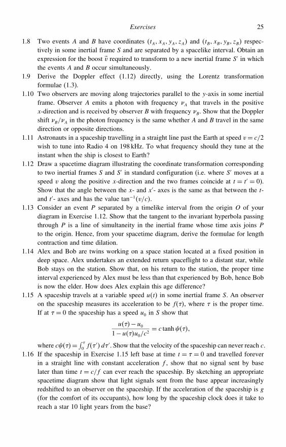
1.8 Two events A and B have coordinates tA xA yA zA and tB xB yB zB respec-tively in some inertial frame S and are separated by a spacelike interval. Obtain anexpression for the boost v required to transform to a new inertial frame S′ in whichthe events A and B occur simultaneously.
1.9 Derive the Doppler effect (1.12) directly, using the Lorentz transformationformulae (1.3).
1.10 Two observers are moving along trajectories parallel to the y-axis in some inertialframe. Observer A emits a photon with frequency A that travels in the positivex-direction and is received by observer B with frequency B. Show that the Dopplershift B/A in the photon frequency is the same whether A and B travel in the samedirection or opposite directions.
1.11 Astronauts in a spaceship travelling in a straight line past the Earth at speed v= c/2wish to tune into Radio 4 on 198 kHz. To what frequency should they tune at theinstant when the ship is closest to Earth?
1.12 Draw a spacetime diagram illustrating the coordinate transformation correspondingto two inertial frames S and S′ in standard configuration (i.e. where S′ moves at aspeed v along the positive x-direction and the two frames coincide at t = t′ = 0).Show that the angle between the x- and x′- axes is the same as that between the t-and t′- axes and has the value tan−1v/c.
1.13 Consider an event P separated by a timelike interval from the origin O of yourdiagram in Exercise 1.12. Show that the tangent to the invariant hyperbola passingthrough P is a line of simultaneity in the inertial frame whose time axis joins P
to the origin. Hence, from your spacetime diagram, derive the formulae for lengthcontraction and time dilation.
1.14 Alex and Bob are twins working on a space station located at a fixed position indeep space. Alex undertakes an extended return spaceflight to a distant star, whileBob stays on the station. Show that, on his return to the station, the proper timeinterval experienced by Alex must be less than that experienced by Bob, hence Bobis now the elder. How does Alex explain this age difference?
1.15 A spaceship travels at a variable speed ut in some inertial frame S. An observeron the spaceship measures its acceleration to be f, where is the proper time.If at = 0 the spaceship has a speed u0 in S show that
u−u0
1−uu0/c2= c tanh
where c= ∫
0 f′d ′. Show that the velocity of the spaceship can never reach c.
1.16 If the spaceship in Exercise 1.15 left base at time t = = 0 and travelled foreverin a straight line with constant acceleration f , show that no signal sent by baselater than time t = c/f can ever reach the spaceship. By sketching an appropriatespacetime diagram show that light signals sent from the base appear increasinglyredshifted to an observer on the spaceship. If the acceleration of the spaceship is g(for the comfort of its occupants), how long by the spaceship clock does it take toreach a star 10 light years from the base?
2
Manifolds and coordinates
Our discussion of special relativity has led us to model the physical world as afour-dimensional continuum, called spacetime, with a Minkowski geometry. Thisis an example of a manifold. As we shall see, the more complicated spacetimegeometries of general relativity are also examples of manifolds. It is thereforeworthwhile discussing manifolds in general. In the following we consider generalproperties of manifolds commonly encountered in physics, and we concentrate inparticular on Riemannian manifolds, which will be central to our discussion ofgeneral relativity.
2.1 The concept of a manifold
In general, a manifold is any set that can be continuously parameterised. Thenumber of independent parameters required to specify any point in the set uniquelyis the dimension of the manifold, and the parameters themselves are the coor-dinates of the manifold. An abstract example is the set of all rigid rotations ofCartesian coordinate systems in three-dimensional Euclidean space, which can beparameterised by the Euler angles. So the set of rotations is a three-dimensionalmanifold: each point is a particular rotation, and the coordinates of the pointare the three Euler angles. Similarly, the phase space of a particle in classicalmechanics can be parameterised by three position coordinates q1 q2 q3 andthree momentum coordinates p1 p2 p3, and thus the set of points in this phasespace forms a six-dimensional manifold. In fact, one can regard ‘manifold’ as justa fancy word for ‘space’ in the general mathematical sense.
In its most primitive form a general manifold is simply an amorphous collectionof points. Most manifolds used in physics, however, are ‘differential manifolds’,which are continuous and differentiable in the following way. A manifold iscontinuous if, in the neighbourhood of every point P, there are other points whosecoordinates differ infinitesimally from those of P. A manifold is differentiable ifit is possible to define a scalar field at each point of the manifold that can bedifferentiated everywhere. Both our examples above are differential manifolds.
26
2.3 Curves and surfaces 27
The association of points with the values of their parameters can be thought ofas a mapping of the points of a manifold into points of the Euclidean space of thesame dimension. This means that ‘locally’ a manifold looks like the correspondingEuclidean space: it is ‘smooth’ and has a certain number of dimensions.
2.2 Coordinates
An N -dimensional manifold of points is one for which N independent realcoordinates x1 x2 xN are required to specify any point completely.1 TheseN coordinates are entirely general and are denoted collectively by xa, where it isunderstood that a= 12 N .
As a technical point, we should mention that in general it may not be possibleto cover the whole manifold with only one non-degenerate coordinate system,namely, one which ascribes a unique set of N coordinate values to each point,so that the correspondence between points and sets of coordinate values (labels)is one-to-one. Let us consider, for example, the points that constitute a plane.These points clearly form a two-dimensional manifold (called R2). An exampleof a degenerate coordinate system on this manifold is the polar coordinates rin the plane, which have a degeneracy at the origin because is indeterminatethere. For this manifold, we could avoid the degeneracy at the origin by using,for example, Cartesian coordinates. For a general manifold, however, we mighthave no choice in the matter and might have to work with coordinate systems thatcover only a portion of the manifold, called coordinate patches. For example, theset of points making up the surface of a sphere forms a two-dimensional manifold(called S2). This manifold is usually ‘parameterised’ by the coordinates and, but is degenerate at the poles. In this case, however, it can be shown thatthere is no coordinate system that covers the whole of S2 without degeneracy; thesmallest number of patches needed is two. In general, a set of coordinate patchesthat covers the whole manifold is called an atlas.
Thus, in general, we do not require the whole of a manifold to be coveredby a single coordinate system. Instead, we may have a collection of coordinatesystems, each covering some part of , and all these are on an equal footing.We do not regard any one coordinate system as in some way preferred.
2.3 Curves and surfaces
Given a manifold, we shall be concerned with points in it and with subsets ofpoints that define curves and surfaces. We shall frequently define these curves
1 The reason why the coordinates are written with superscripts rather than subscripts will become clear later.
28 Manifolds and coordinates
and surfaces parametrically. Thus, since a curve has one degree of freedom,it depends on one parameter and so we define a curve in the manifold by theparametric equations
xa = xau a= 12 N
where u is some parameter and x1u x2u xN u denote N functions of u.Similarly, since a submanifold or surface of M dimensions M < N has M
degrees of freedom, it depends on M parameters and is given by the N parametricequations
xa = xau1 u2 uM a= 12 N (2.1)
If, in particular, M = N −1 then the submanifold is called a hypersurface. In thiscase, the N −1 parameters can be eliminated from these N equations to give oneequation relating the coordinates, i.e.
fx1 x2 xN = 0
From a different but equivalent point of view, a point in a manifold is charac-terised by N coordinates. If the point is restricted to lie in a particular hypersurface,i.e. an N − 1-dimensional subspace, then the point’s coordinates must satisfyone constraint equation, namely
fx1 x2 xN = 0
Similarly, points in an M-dimensional subspace M < N must satisfy N −M
constraints
f1x1 x2 xN = 0
f2x1 x2 xN = 0
fN−Mx1 x2 xM = 0
which is an alternative to the parametric representation (2.1).
2.4 Coordinate transformations
To locate a point in a manifold we use a system of N coordinates, but the choice ofthese coordinates is arbitrary. The important idea is not the ‘labels’ but the pointsthemselves and the geometrical and topological relationships between them.
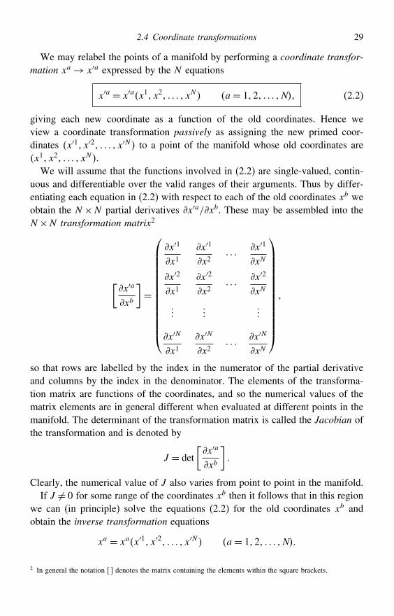
2.4 Coordinate transformations 29
We may relabel the points of a manifold by performing a coordinate transfor-mation xa→ x′a expressed by the N equations
x′a = x′ax1 x2 xN a= 12 N (2.2)
giving each new coordinate as a function of the old coordinates. Hence weview a coordinate transformation passively as assigning the new primed coor-dinates x′1 x′2 x′N to a point of the manifold whose old coordinates arex1 x2 xN .
We will assume that the functions involved in (2.2) are single-valued, contin-uous and differentiable over the valid ranges of their arguments. Thus by differ-entiating each equation in (2.2) with respect to each of the old coordinates xb weobtain the N ×N partial derivatives x′a/xb. These may be assembled into theN ×N transformation matrix2
[x′a
xb
]=
⎛⎜⎜⎜⎜⎜⎜⎜⎜⎜⎜⎜⎜⎜⎝
x′1
x1x′1
x2· · · x′1
xN
x′2
x1x′2
x2· · · x′2
xN
x′N
x1x′N
x2· · · x′N
xN
⎞⎟⎟⎟⎟⎟⎟⎟⎟⎟⎟⎟⎟⎟⎠
so that rows are labelled by the index in the numerator of the partial derivativeand columns by the index in the denominator. The elements of the transforma-tion matrix are functions of the coordinates, and so the numerical values of thematrix elements are in general different when evaluated at different points in themanifold. The determinant of the transformation matrix is called the Jacobian ofthe transformation and is denoted by
J = det[x′a
xb
]
Clearly, the numerical value of J also varies from point to point in the manifold.If J = 0 for some range of the coordinates xb then it follows that in this region
we can (in principle) solve the equations (2.2) for the old coordinates xb andobtain the inverse transformation equations
xa = xax′1 x′2 x′N a= 12 N
2 In general the notation denotes the matrix containing the elements within the square brackets.
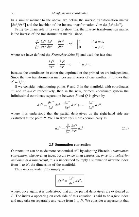
30 Manifolds and coordinates
In a similar manner to the above, we define the inverse transformation matrix xa/x′b and the Jacobian of the inverse transformation J ′ = det xa/x′b.
Using the chain rule, it is easy to show that the inverse transformation matrixis the inverse of the transformation matrix, since
N∑b=1
x′a
xbxb
x′c= x′a
x′c= ac =
1 if a= c
0 if a = c
where we have defined the Kronecker delta ac and used the fact that
x′a
x′c= xa
xc= 0 if a = c
because the coordinates in either the unprimed or the primed set are independent.Since the two transformation matrices are inverses of one another, it follows thatJ ′ = 1/J .
If we consider neighbouring points P and Q in the manifold, with coordinatesxa and xa+ dxa respectively, then in the new, primed, coordinate system theinfinitesimal coordinate separation between P and Q is given by
dx′a = x′a
x1dx1+ x′a
x2dx2+· · ·+ x′a
xNdxN
where it is understood that the partial derivatives on the right-hand side areevaluated at the point P. We can write this more economically as
dx′a =N∑b=1
x′a
xbdxb (2.3)
2.5 Summation convention
Our notation can be made more economical still by adopting Einstein’s summationconvention: whenever an index occurs twice in an expression, once as a subscriptand once as a superscript, this is understood to imply a summation over the indexfrom 1 to N , the dimension of the manifold.
Thus we can write (2.3) simply as
dx′a = x′a
xbdxb
where, once again, it is understood that all the partial derivatives are evaluated atP. The index a appearing on each side of this equation is said to be a free indexand may take on separately any value from 1 to N . We consider a superscript that
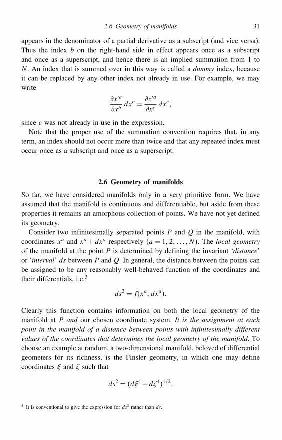
2.6 Geometry of manifolds 31
appears in the denominator of a partial derivative as a subscript (and vice versa).Thus the index b on the right-hand side in effect appears once as a subscriptand once as a superscript, and hence there is an implied summation from 1 toN . An index that is summed over in this way is called a dummy index, becauseit can be replaced by any other index not already in use. For example, we maywrite
x′a
xbdxb = x′a
xcdxc
since c was not already in use in the expression.Note that the proper use of the summation convention requires that, in any
term, an index should not occur more than twice and that any repeated index mustoccur once as a subscript and once as a superscript.
2.6 Geometry of manifolds
So far, we have considered manifolds only in a very primitive form. We haveassumed that the manifold is continuous and differentiable, but aside from theseproperties it remains an amorphous collection of points. We have not yet definedits geometry.
Consider two infinitesimally separated points P and Q in the manifold, withcoordinates xa and xa+dxa respectively a = 12 N. The local geometryof the manifold at the point P is determined by defining the invariant ‘distance’or ‘interval’ ds between P and Q. In general, the distance between the points canbe assigned to be any reasonably well-behaved function of the coordinates andtheir differentials, i.e.3
ds2 = fxadxa
Clearly this function contains information on both the local geometry of themanifold at P and our chosen coordinate system. It is the assignment at eachpoint in the manifold of a distance between points with infinitesimally differentvalues of the coordinates that determines the local geometry of the manifold. Tochoose an example at random, a two-dimensional manifold, beloved of differentialgeometers for its richness, is the Finsler geometry, in which one may definecoordinates and such that
ds2 = d4+d41/2
3 It is conventional to give the expression for ds2 rather than ds.
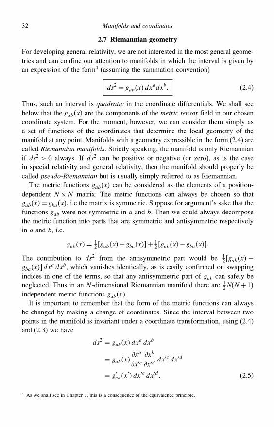
32 Manifolds and coordinates
2.7 Riemannian geometry
For developing general relativity, we are not interested in the most general geome-tries and can confine our attention to manifolds in which the interval is given byan expression of the form4 (assuming the summation convention)
ds2 = gabxdxadxb (2.4)
Thus, such an interval is quadratic in the coordinate differentials. We shall seebelow that the gabx are the components of the metric tensor field in our chosencoordinate system. For the moment, however, we can consider them simply asa set of functions of the coordinates that determine the local geometry of themanifold at any point. Manifolds with a geometry expressible in the form (2.4) arecalled Riemannian manifolds. Strictly speaking, the manifold is only Riemannianif ds2 > 0 always. If ds2 can be positive or negative (or zero), as is the casein special relativity and general relativity, then the manifold should properly becalled pseudo-Riemannian but is usually simply referred to as Riemannian.
The metric functions gabx can be considered as the elements of a position-dependent N ×N matrix. The metric functions can always be chosen so thatgabx= gbax, i.e the matrix is symmetric. Suppose for argument’s sake that thefunctions gab were not symmetric in a and b. Then we could always decomposethe metric function into parts that are symmetric and antisymmetric respectivelyin a and b, i.e.
gabx= 12 gabx+gbax+ 1
2 gabx−gbax
The contribution to ds2 from the antisymmetric part would be 12 gabx−
gbaxdxa dxb, which vanishes identically, as is easily confirmed on swapping
indices in one of the terms, so that any antisymmetric part of gab can safely beneglected. Thus in an N -dimensional Riemannian manifold there are 1
2NN +1independent metric functions gabx.It is important to remember that the form of the metric functions can always
be changed by making a change of coordinates. Since the interval between twopoints in the manifold is invariant under a coordinate transformation, using (2.4)and (2.3) we have
ds2 = gabxdxa dxb
= gabxxa
x′cxb
x′ddx′c dx′d
= g′cdx′dx′c dx′d (2.5)
4 As we shall see in Chapter 7, this is a consequence of the equivalence principle.
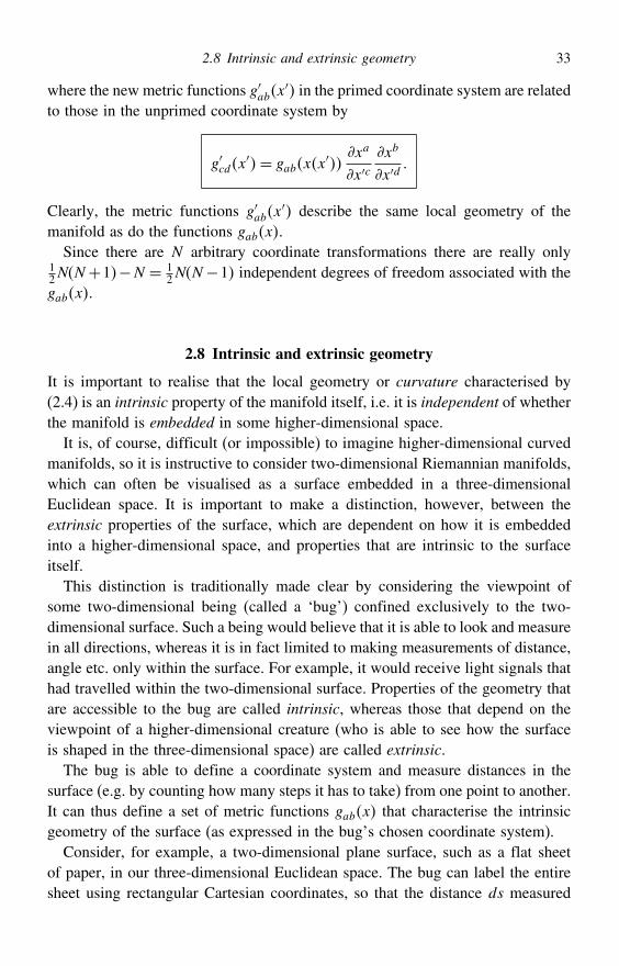
2.8 Intrinsic and extrinsic geometry 33
where the new metric functions g′abx′ in the primed coordinate system are related
to those in the unprimed coordinate system by
g′cdx′= gabxx
′xa
x′cxb
x′d
Clearly, the metric functions g′abx′ describe the same local geometry of the
manifold as do the functions gabx.Since there are N arbitrary coordinate transformations there are really only
12NN +1−N = 1
2NN −1 independent degrees of freedom associated with thegabx.
2.8 Intrinsic and extrinsic geometry
It is important to realise that the local geometry or curvature characterised by(2.4) is an intrinsic property of the manifold itself, i.e. it is independent of whetherthe manifold is embedded in some higher-dimensional space.
It is, of course, difficult (or impossible) to imagine higher-dimensional curvedmanifolds, so it is instructive to consider two-dimensional Riemannian manifolds,which can often be visualised as a surface embedded in a three-dimensionalEuclidean space. It is important to make a distinction, however, between theextrinsic properties of the surface, which are dependent on how it is embeddedinto a higher-dimensional space, and properties that are intrinsic to the surfaceitself.
This distinction is traditionally made clear by considering the viewpoint ofsome two-dimensional being (called a ‘bug’) confined exclusively to the two-dimensional surface. Such a being would believe that it is able to look and measurein all directions, whereas it is in fact limited to making measurements of distance,angle etc. only within the surface. For example, it would receive light signals thathad travelled within the two-dimensional surface. Properties of the geometry thatare accessible to the bug are called intrinsic, whereas those that depend on theviewpoint of a higher-dimensional creature (who is able to see how the surfaceis shaped in the three-dimensional space) are called extrinsic.
The bug is able to define a coordinate system and measure distances in thesurface (e.g. by counting how many steps it has to take) from one point to another.It can thus define a set of metric functions gabx that characterise the intrinsicgeometry of the surface (as expressed in the bug’s chosen coordinate system).
Consider, for example, a two-dimensional plane surface, such as a flat sheetof paper, in our three-dimensional Euclidean space. The bug can label the entiresheet using rectangular Cartesian coordinates, so that the distance ds measured
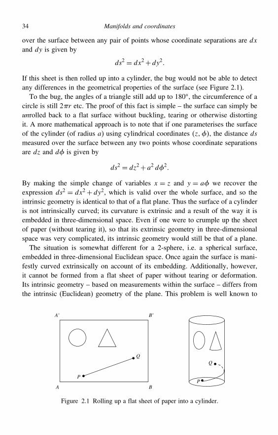
34 Manifolds and coordinates
over the surface between any pair of points whose coordinate separations are dxand dy is given by
ds2 = dx2+dy2
If this sheet is then rolled up into a cylinder, the bug would not be able to detectany differences in the geometrical properties of the surface (see Figure 2.1).
To the bug, the angles of a triangle still add up to 180, the circumference of acircle is still 2r etc. The proof of this fact is simple – the surface can simply beunrolled back to a flat surface without buckling, tearing or otherwise distortingit. A more mathematical approach is to note that if one parameterises the surfaceof the cylinder (of radius a) using cylindrical coordinates z, the distance dsmeasured over the surface between any two points whose coordinate separationsare dz and d is given by
ds2 = dz2+a2 d2
By making the simple change of variables x = z and y = a we recover theexpression ds2 = dx2+dy2, which is valid over the whole surface, and so theintrinsic geometry is identical to that of a flat plane. Thus the surface of a cylinderis not intrinsically curved; its curvature is extrinsic and a result of the way it isembedded in three-dimensional space. Even if one were to crumple up the sheetof paper (without tearing it), so that its extrinsic geometry in three-dimensionalspace was very complicated, its intrinsic geometry would still be that of a plane.
The situation is somewhat different for a 2-sphere, i.e. a spherical surface,embedded in three-dimensional Euclidean space. Once again the surface is mani-festly curved extrinsically on account of its embedding. Additionally, however,it cannot be formed from a flat sheet of paper without tearing or deformation.Its intrinsic geometry – based on measurements within the surface – differs fromthe intrinsic (Euclidean) geometry of the plane. This problem is well known to
PP
A
A' B'
B
Figure 2.1 Rolling up a flat sheet of paper into a cylinder.
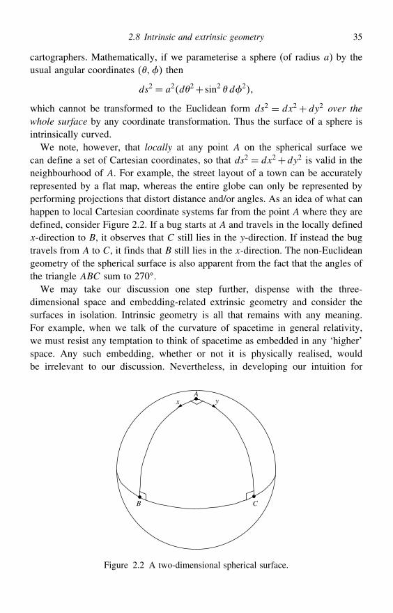
2.8 Intrinsic and extrinsic geometry 35
cartographers. Mathematically, if we parameterise a sphere (of radius a) by theusual angular coordinates then
ds2 = a2d2+ sin2 d2
which cannot be transformed to the Euclidean form ds2 = dx2+dy2 over thewhole surface by any coordinate transformation. Thus the surface of a sphere isintrinsically curved.
We note, however, that locally at any point A on the spherical surface wecan define a set of Cartesian coordinates, so that ds2 = dx2+dy2 is valid in theneighbourhood of A. For example, the street layout of a town can be accuratelyrepresented by a flat map, whereas the entire globe can only be represented byperforming projections that distort distance and/or angles. As an idea of what canhappen to local Cartesian coordinate systems far from the point A where they aredefined, consider Figure 2.2. If a bug starts at A and travels in the locally definedx-direction to B, it observes that C still lies in the y-direction. If instead the bugtravels from A to C, it finds that B still lies in the x-direction. The non-Euclideangeometry of the spherical surface is also apparent from the fact that the angles ofthe triangle ABC sum to 270.We may take our discussion one step further, dispense with the three-
dimensional space and embedding-related extrinsic geometry and consider thesurfaces in isolation. Intrinsic geometry is all that remains with any meaning.For example, when we talk of the curvature of spacetime in general relativity,we must resist any temptation to think of spacetime as embedded in any ‘higher’space. Any such embedding, whether or not it is physically realised, wouldbe irrelevant to our discussion. Nevertheless, in developing our intuition for
C
x y
B
A
Figure 2.2 A two-dimensional spherical surface.
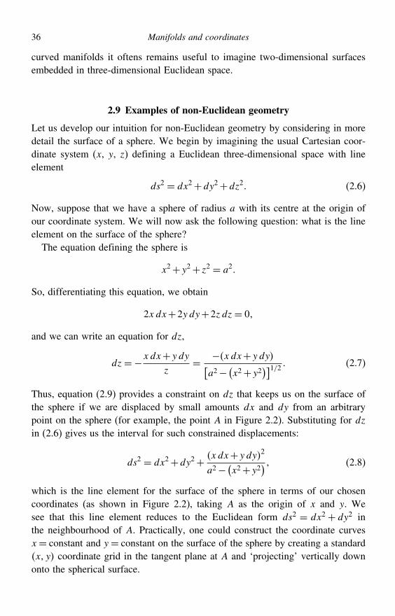
36 Manifolds and coordinates
curved manifolds it oftens remains useful to imagine two-dimensional surfacesembedded in three-dimensional Euclidean space.
2.9 Examples of non-Euclidean geometry
Let us develop our intuition for non-Euclidean geometry by considering in moredetail the surface of a sphere. We begin by imagining the usual Cartesian coor-dinate system (x, y, z) defining a Euclidean three-dimensional space with lineelement
ds2 = dx2+dy2+dz2 (2.6)
Now, suppose that we have a sphere of radius a with its centre at the origin ofour coordinate system. We will now ask the following question: what is the lineelement on the surface of the sphere?
The equation defining the sphere is
x2+y2+ z2 = a2
So, differentiating this equation, we obtain
2xdx+2y dy+2zdz= 0
and we can write an equation for dz,
dz=−xdx+y dy
z= −xdx+y dy[
a2− (x2+y2)]1/2 (2.7)
Thus, equation (2.9) provides a constraint on dz that keeps us on the surface ofthe sphere if we are displaced by small amounts dx and dy from an arbitrarypoint on the sphere (for example, the point A in Figure 2.2). Substituting for dzin (2.6) gives us the interval for such constrained displacements:
ds2 = dx2+dy2+ xdx+y dy2
a2− (x2+y2) (2.8)
which is the line element for the surface of the sphere in terms of our chosencoordinates (as shown in Figure 2.2), taking A as the origin of x and y. Wesee that this line element reduces to the Euclidean form ds2 = dx2 + dy2 inthe neighbourhood of A. Practically, one could construct the coordinate curvesx= constant and y = constant on the surface of the sphere by creating a standardx y coordinate grid in the tangent plane at A and ‘projecting’ vertically downonto the spherical surface.
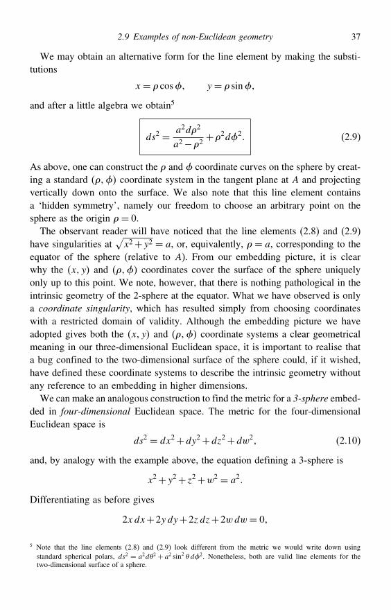
2.9 Examples of non-Euclidean geometry 37
We may obtain an alternative form for the line element by making the substi-tutions
x = cos y = sin
and after a little algebra we obtain5
ds2 = a2d2
a2−2+2d2 (2.9)
As above, one can construct the and coordinate curves on the sphere by creat-ing a standard coordinate system in the tangent plane at A and projectingvertically down onto the surface. We also note that this line element containsa ‘hidden symmetry’, namely our freedom to choose an arbitrary point on thesphere as the origin = 0.
The observant reader will have noticed that the line elements (2.8) and (2.9)have singularities at
√x2+y2 = a, or, equivalently, = a, corresponding to the
equator of the sphere (relative to A). From our embedding picture, it is clearwhy the x y and coordinates cover the surface of the sphere uniquelyonly up to this point. We note, however, that there is nothing pathological in theintrinsic geometry of the 2-sphere at the equator. What we have observed is onlya coordinate singularity, which has resulted simply from choosing coordinateswith a restricted domain of validity. Although the embedding picture we haveadopted gives both the x y and coordinate systems a clear geometricalmeaning in our three-dimensional Euclidean space, it is important to realise thata bug confined to the two-dimensional surface of the sphere could, if it wished,have defined these coordinate systems to describe the intrinsic geometry withoutany reference to an embedding in higher dimensions.
We can make an analogous construction to find the metric for a 3-sphere embed-ded in four-dimensional Euclidean space. The metric for the four-dimensionalEuclidean space is
ds2 = dx2+dy2+dz2+dw2 (2.10)
and, by analogy with the example above, the equation defining a 3-sphere is
x2+y2+ z2+w2 = a2
Differentiating as before gives
2xdx+2y dy+2zdz+2wdw = 0
5 Note that the line elements (2.8) and (2.9) look different from the metric we would write down usingstandard spherical polars, ds2 = a2d2 + a2 sin2 d2. Nonetheless, both are valid line elements for thetwo-dimensional surface of a sphere.
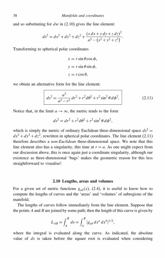
38 Manifolds and coordinates
and so substituting for dw in (2.10) gives the line element:
ds2 = dx2+dy2+dz2+ xdx+y dy+ zdz2
a2− (x2+y2+ z2)
Transforming to spherical polar coordinates
x = r sin cos
y = r sin sin
z = r cos
we obtain an alternative form for the line element:
ds2 = a2
a2− r2dr2+ r2d2+ r2 sin2 d2 (2.11)
Notice that, in the limit a→, the metric tends to the form
ds2 = dr2+ r2d2+ r2 sin2 d2
which is simply the metric of ordinary Euclidean three-dimensional space ds2 =dx2+dy2+dz2, rewritten in spherical polar coordinates. The line element (2.11)therefore describes a non-Euclidean three-dimensional space. We note that thisline element also has a singularity, this time at r = a. As one might expect fromour discussion above, this is once again just a coordinate singularity, although ourexistence as three-dimensional ‘bugs’ makes the geometric reason for this lessstraightforward to visualise!
2.10 Lengths, areas and volumes
For a given set of metric functions gabx, (2.4), it is useful to know how tocompute the lengths of curves and the ‘areas’ and ‘volumes’ of subregions of themanifold.
The lengths of curves follow immediately from the line element. Suppose thatthe points A and B are joined by some path; then the length of this curve is given by
LAB =∫ B
Ads =
∫ B
Agab dxa dxb1/2
where the integral is evaluated along the curve. As indicated, the absolutevalue of ds is taken before the square root is evaluated when considering
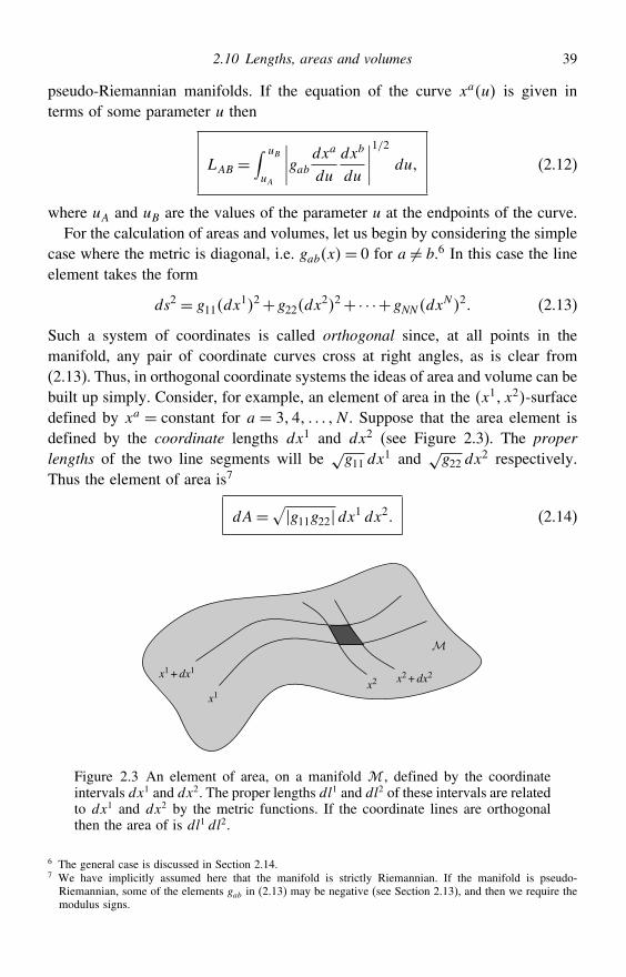
2.10 Lengths, areas and volumes 39
pseudo-Riemannian manifolds. If the equation of the curve xau is given interms of some parameter u then
LAB =∫ uB
uA
∣∣∣∣gab dxadu
dxb
du
∣∣∣∣1/2 du (2.12)
where uA and uB are the values of the parameter u at the endpoints of the curve.For the calculation of areas and volumes, let us begin by considering the simple
case where the metric is diagonal, i.e. gabx= 0 for a = b.6 In this case the lineelement takes the form
ds2 = g11dx12+g22dx
22+· · ·+gNN dxN 2 (2.13)
Such a system of coordinates is called orthogonal since, at all points in themanifold, any pair of coordinate curves cross at right angles, as is clear from(2.13). Thus, in orthogonal coordinate systems the ideas of area and volume can bebuilt up simply. Consider, for example, an element of area in the x1 x2-surfacedefined by xa = constant for a = 34 N . Suppose that the area element isdefined by the coordinate lengths dx1 and dx2 (see Figure 2.3). The properlengths of the two line segments will be
√g11 dx
1 and√g22 dx
2 respectively.Thus the element of area is7
dA=√g11g22dx1 dx2 (2.14)
x2x1 + dx1
x1
x2 + dx2
Figure 2.3 An element of area, on a manifold , defined by the coordinateintervals dx1 and dx2. The proper lengths dl1 and dl2 of these intervals are relatedto dx1 and dx2 by the metric functions. If the coordinate lines are orthogonalthen the area of is dl1 dl2.
6 The general case is discussed in Section 2.14.7 We have implicitly assumed here that the manifold is strictly Riemannian. If the manifold is pseudo-Riemannian, some of the elements gab in (2.13) may be negative (see Section 2.13), and then we require themodulus signs.
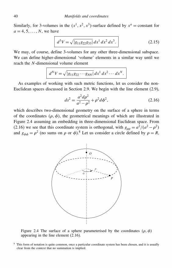
40 Manifolds and coordinates
Similarly, for 3-volumes in the x1 x2 x3-surface defined by xa = constant fora= 45 N , we have
d3V =√g11g22g33dx1 dx2 dx3 (2.15)
We may, of course, define 3-volumes for any other three-dimensional subspace.We can define higher-dimensional ‘volume’ elements in a similar way until wereach the N -dimensional volume element
dNV =√g11g22 · · ·gNN dx1 dx2 · · · dxN As examples of working with such metric functions, let us consider the non-
Euclidean spaces discussed in Section 2.9. We begin with the line element (2.9),
ds2 = a2d2
a2−2+2d2 (2.16)
which describes two-dimensional geometry on the surface of a sphere in termsof the coordinates , the geometrical meanings of which are illustrated inFigure 2.4 assuming an embedding in three-dimensional Euclidean space. From(2.16) we see that this coordinate system is orthogonal, with g = a2/a2−2
and g = 2 (no sums on or ).8 Let us consider a circle defined by = R,
ρ
P
O
φ
Figure 2.4 The surface of a sphere parameterised by the coordinates appearing in the line element (2.16).
8 This form of notation is quite common, once a particular coordinate system has been chosen, and it is usuallyclear from the context that no summation is implied.
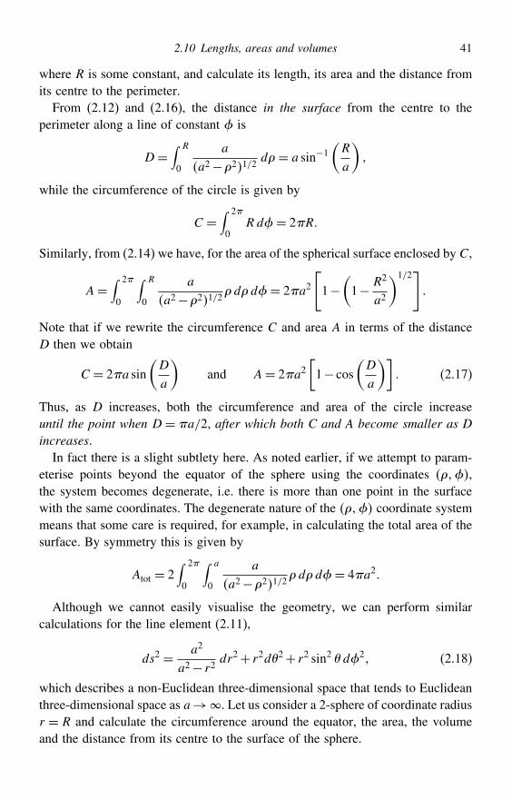
2.10 Lengths, areas and volumes 41
where R is some constant, and calculate its length, its area and the distance fromits centre to the perimeter.
From (2.12) and (2.16), the distance in the surface from the centre to theperimeter along a line of constant is
D =∫ R
0
a
a2−21/2d= a sin−1
(R
a
)
while the circumference of the circle is given by
C =∫ 2
0Rd= 2R
Similarly, from (2.14) we have, for the area of the spherical surface enclosed by C,
A=∫ 2
0
∫ R
0
a
a2−21/2dd= 2a2
[1−
(1− R2
a2
)1/2]
Note that if we rewrite the circumference C and area A in terms of the distanceD then we obtain
C = 2a sin(D
a
)and A= 2a2
[1− cos
(D
a
)] (2.17)
Thus, as D increases, both the circumference and area of the circle increaseuntil the point when D = a/2, after which both C and A become smaller as Dincreases.
In fact there is a slight subtlety here. As noted earlier, if we attempt to param-eterise points beyond the equator of the sphere using the coordinates ,the system becomes degenerate, i.e. there is more than one point in the surfacewith the same coordinates. The degenerate nature of the coordinate systemmeans that some care is required, for example, in calculating the total area of thesurface. By symmetry this is given by
Atot = 2∫ 2
0
∫ a
0
a
a2−21/2dd= 4a2
Although we cannot easily visualise the geometry, we can perform similarcalculations for the line element (2.11),
ds2 = a2
a2− r2dr2+ r2d2+ r2 sin2 d2 (2.18)
which describes a non-Euclidean three-dimensional space that tends to Euclideanthree-dimensional space as a→. Let us consider a 2-sphere of coordinate radiusr = R and calculate the circumference around the equator, the area, the volumeand the distance from its centre to the surface of the sphere.
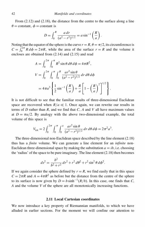
42 Manifolds and coordinates
From (2.12) and (2.18), the distance from the centre to the surface along a line = constant, = constant is
D =∫ R
0
adr
a2− r21/2= a sin−1
(R
a
)
Noting that the equator of the sphere is the curve r =R, =/2, its circumference isC = ∫ 2
0 Rd = 2R while the area of the surface r = R and the volume itencloses are obtained from (2.14) and (2.15) and read
A =∫ 2
0
∫
0R2 sin dd= 4R2
V =∫ 2
0
∫
0
∫ R
0
ar2 sin a2− r21/2
dr dd
= 4a3
⎧⎨⎩12sin−1
(R
a
)+ R
a
[1−
(R
a
)2]1/2⎫⎬⎭
It is not difficult to see that the familiar results of three-dimensional Euclideanspace are recovered when R/a 1. Once again, we can rewrite our results interms of D rather than R, and we find that C, A and V all have maximum valuesat D = a/2. By analogy with the above two-dimensional example, the totalvolume of this space is
Vtot = 2∫ 2
0
∫
0
∫ a
0
ar2 sin a2− r21/2
dr dd= 22a3
The three-dimensional non-Euclidean space described by the line element (2.18)thus has a finite volume. We can generate a line element for an infinite non-Euclidean three-dimensional space by making the substitution a= ib, i.e. choosingthe ‘radius’ of the space to be pure imaginary. The line element (2.18) then becomes
ds2 = b2
b2+ r2dr2+ r2 d2+ r2 sin2 d2
If we again consider the sphere defined by r =R, we find easily that in this spaceC = 2R and A= 4R2 as before but the distance from the centre of the sphereto its surface is now given by D = b sinh−1R/b. In this case, one finds that C,A and the volume V of the sphere are all monotonically increasing functions.
2.11 Local Cartesian coordinates
We now introduce a key property of Riemannian manifolds, to which we havealluded in earlier sections. For the moment we will confine our attention to
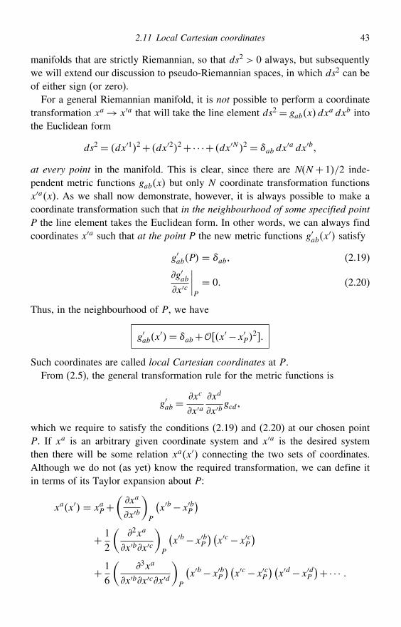
2.11 Local Cartesian coordinates 43
manifolds that are strictly Riemannian, so that ds2 > 0 always, but subsequentlywe will extend our discussion to pseudo-Riemannian spaces, in which ds2 can beof either sign (or zero).
For a general Riemannian manifold, it is not possible to perform a coordinatetransformation xa→ x′a that will take the line element ds2 = gabxdx
a dxb intothe Euclidean form
ds2 = dx′12+ dx′22+· · ·+ dx′N 2 = ab dx′a dx′b
at every point in the manifold. This is clear, since there are NN + 1/2 inde-pendent metric functions gabx but only N coordinate transformation functionsx′ax. As we shall now demonstrate, however, it is always possible to make acoordinate transformation such that in the neighbourhood of some specified pointP the line element takes the Euclidean form. In other words, we can always findcoordinates x′a such that at the point P the new metric functions g′abx
′ satisfy
g′abP = ab (2.19)
g′abx′c
∣∣∣∣P
= 0 (2.20)
Thus, in the neighbourhood of P, we have
g′abx′= ab+ x′ −x′P
2
Such coordinates are called local Cartesian coordinates at P.From (2.5), the general transformation rule for the metric functions is
g′ab =xc
x′axd
x′bgcd
which we require to satisfy the conditions (2.19) and (2.20) at our chosen pointP. If xa is an arbitrary given coordinate system and x′a is the desired systemthen there will be some relation xax′ connecting the two sets of coordinates.Although we do not (as yet) know the required transformation, we can define itin terms of its Taylor expansion about P:
xax′ = xaP+(xa
x′b
)P
(x′b−x′bP
)+ 1
2
(2xa
x′bx′c
)P
(x′b−x′bP
) (x′c−x′cP
)+ 1
6
(3xa
x′bx′cx′d
)P
(x′b−x′bP
) (x′c−x′cP
) (x′d−x′dP
)+· · ·
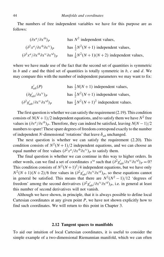
44 Manifolds and coordinates
The numbers of free independent variables we have for this purpose are asfollows:
xa/x′bP has N 2 independent values
2xa/x′bx′cP has 12N
2N +1 independent values
3xa/x′bx′cx′dP has 16N
2N +1N +2 independent values
where we have made use of the fact that the second set of quantities is symmetricin b and c and the third set of quantities is totally symmetric in b, c and d. Wemay compare this with the number of independent parameters we may want to fix:
g′abP has 12NN +1 independent values
g′ab/x′cP has 1
2N2N +1 independent values
2g′ab/x′cx′dP has 1
4N2N +12 independent values
The first question is whetherwe can satisfy the requirement (2.19). This conditionconsists ofNN +1/2 independent equations, and to satisfy them we haveN 2 freevalues in xa/x′bP . Therefore, they can indeed be satisfied, leaving NN −1/2numbers to spare! These spare degrees of freedom correspond exactly to the numberof independentN -dimensional ‘rotations’ that leave ab unchanged.The next question is whether we can satisfy the requirement (2.20). This
condition consists of N 2N +1/2 independent equations, and we can choose anequal number of free values 2xa/x′bx′cP to satisfy them.The final question is whether we can continue in this way to higher orders. In
other words, can we find a set of coordinates x′a such that 2g′ab/x′cx′dP = 0?
This condition consists of N 2N +12/4 independent equations, but we have onlyN 2N +1N +2/6 free values in 2g′ab/x
′cx′dP , so these equations cannotin general be satisfied. This means that there are N 2N 2− 1/12 ‘degrees offreedom’ among the second derivatives 2g′ab/x
′cx′dP , i.e. in general at leastthis number of second derivatives will not vanish.
Although we have shown, in principle, that it is always possible to define localCartesian coordinates at any given point P, we have not shown explicitly how tofind such coordinates. We will return to this point in Chapter 3.
2.12 Tangent spaces to manifolds
To aid our intuition of local Cartesian coordinates, it is useful to consider thesimple example of a two-dimensional Riemannian manifold, which we can often
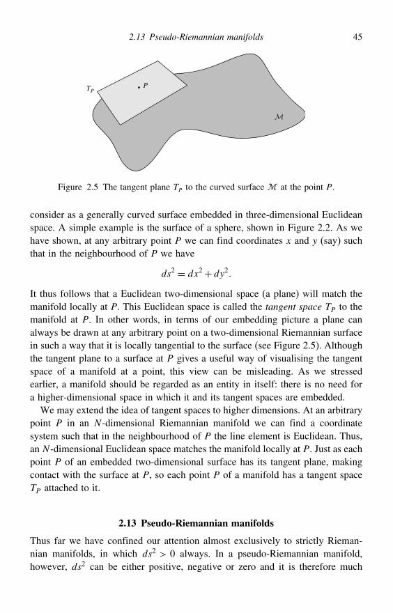
2.13 Pseudo-Riemannian manifolds 45
TPP
Figure 2.5 The tangent plane TP to the curved surface at the point P.
consider as a generally curved surface embedded in three-dimensional Euclideanspace. A simple example is the surface of a sphere, shown in Figure 2.2. As wehave shown, at any arbitrary point P we can find coordinates x and y (say) suchthat in the neighbourhood of P we have
ds2 = dx2+dy2
It thus follows that a Euclidean two-dimensional space (a plane) will match themanifold locally at P. This Euclidean space is called the tangent space TP to themanifold at P. In other words, in terms of our embedding picture a plane canalways be drawn at any arbitrary point on a two-dimensional Riemannian surfacein such a way that it is locally tangential to the surface (see Figure 2.5). Althoughthe tangent plane to a surface at P gives a useful way of visualising the tangentspace of a manifold at a point, this view can be misleading. As we stressedearlier, a manifold should be regarded as an entity in itself: there is no need fora higher-dimensional space in which it and its tangent spaces are embedded.
We may extend the idea of tangent spaces to higher dimensions. At an arbitrarypoint P in an N -dimensional Riemannian manifold we can find a coordinatesystem such that in the neighbourhood of P the line element is Euclidean. Thus,an N -dimensional Euclidean space matches the manifold locally at P. Just as eachpoint P of an embedded two-dimensional surface has its tangent plane, makingcontact with the surface at P, so each point P of a manifold has a tangent spaceTP attached to it.
2.13 Pseudo-Riemannian manifolds
Thus far we have confined our attention almost exclusively to strictly Rieman-nian manifolds, in which ds2 > 0 always. In a pseudo-Riemannian manifold,however, ds2 can be either positive, negative or zero and it is therefore much
46 Manifolds and coordinates
harder to visualise even two-dimensional manifolds of this type. Nevertheless,the mathematical tools we have developed so far are straightforwardly applied topseudo-Riemannian manifolds with little modification.
The simplest way to understand pseudo-Riemannian manifolds is to considerthe transformation to local ‘Cartesian’ coordinates at some arbitrary point P. Youwill notice from Section 2.11 that our argument showing that the condition (2.20)holds for the derivatives of the metric functions in a Riemannian manifold canbe extended immediately to the pseudo-Riemannian case. Let us assume thatthe coordinate system xa already satisfies this condition. However, the condition(2.19) on the values of the metric functions themselves requires further investi-gation. Let us now attempt to obtain a new coordinate system x′a in which (2.19)is also satisfied. We note in passing that, in order for (2.20) to remain valid, thenew coordinates x′a must be related to the old ones xa by a linear transformation,x′a = Xa
bxb, where the Xa
b are constants.In general, at a point P the metric functions in the new coordinate system are
given in terms of the original metric functions by
g′abP=(xc
x′a
)P
(xd
x′b
)P
gcdP (2.21)
Let us define symmetric matrices G and G′ having elements gabP and g′abPrespectively. Similarly, we can define a matrix X having elements xa/x′bP .Then, in matrix notation, (2.21) can be written as
G′ = XTGX
Since G is symmetric, it can be diagonalised by this similarity transformation,provided that we choose the columns of X to be the normalised eigenvectorsof G. Then G′ = diag12 N , where a is the ath eigenvalue of G (theeigenvalues must all be real).
In a strictly Riemannian manifold, ds2 = gab dxadxb is always positive at any
point P. Thus the matrix G≡ gab at any point must be positive definite, i.e. allits eigenvalues must be positive. At an arbitrary point in a pseudo-Riemannianmanifold, however, ds2 can be positive, negative or zero, depending on thedirection in which one moves from P. Correspondingly, some of the eigenvaluesof G are negative.
If we now scale our coordinates according to x′a→ x′a/√a (note that here
there is no sum on a), we obtain at the point P
G′ = diag±1±1 ±1where the + and − signs depend on whether the corresponding eigenvalue ispositive or negative. Thus, at any arbitrary point P in a pseudo-Riemannian
2.14 Integration over general submanifolds 47
manifold, it is always possible to find a coordinate system x′a such that in theneighbourhood of P we have
g′abx′= ab+ x′ −x′P
2
where ab = diag±1±1 ±1. The number of positive entries minus thenumber of negative entries in ab is called the signature of the manifold and isthe same at all points.
It follows that, at any arbitrary point P in a pseudo-Riemannian manifold, anN -dimensional space with line element
ds2 =±dx12± dx22±· · ·± dxN 2
will match the manifold locally at P. Such a space is called pseudo-Euclidean andis the tangent space TP to the pseudo-Riemannian manifold at P. An example of apseudo-Euclidean space is the four-dimensional Minkowski spacetime of specialrelativity, which has the line element
ds2 = dct2−dx2−dy2−dz2
when expressed in coordinates corresponding to a Cartesian inertial frame.Minkowski spacetime thus has a signature of −2.
2.14 Integration over general submanifolds
In Section 2.10, we restricted our calculation of ‘volumes’ to coordinate systemsxa that were orthogonal and to submanifolds that were obtained simply by allowingsome of the coordinates to be constants. In fact neither of these simplifications isnecessary, and we are now in a position to consider the general case.
Let us begin by calculating the full N -dimensional volume element dNV in anN -dimensional (pseudo-)Riemannian manifold. From Section 2.10, we know thatif we are working in an orthogonal coordinate system then this volume elementis given by
dNV =√g11g22 · · ·gNN dx1dx2 · · ·dxN For such a coordinate system the matrix G is given by
G≡ gab= diagg11 g22 gNN
so that its determinant is simply the product of the diagonal elements,
detG= g11g22 · · ·gNN
48 Manifolds and coordinates
It is usual to denote detG simply by the symbol g. Thus, we may rewrite thevolume element as
dNV =√gdx1dx2 · · ·dxN (2.22)
What we will now show is that this expression remains valid for an arbitrarycoordinate system.
The key to proving the general result (2.22) for the volume element at somearbitrary point P in the manifold is to transform to local Cartesian coordinatesx′a at P. We know that a small N -dimensional region at P will have volumedNV = dx′1dx′2 · · ·dx′N . In any other general coordinate system xa it is a well-known result that
dx′1dx′2 · · ·dx′N = J dx1dx2 · · ·dxN (2.23)
where the Jacobian factor J is given by
J = det[x′a
xb
]
If, as in Section 2.13, we use X to denote the transformation matrix xa/x′b thenJ = detX−1= detX−1. Defining matrices G and G′ as those having elementsgabP and g′abP respectively, we have (see Section 2.13)
G′ = XTGX (2.24)
Taking determinants of both sides of (2.24) and denoting detG by g and detG′by g′ we obtain
g′ = detX2g = 1J2
g
Since the x′a are locally Cartesian coordinates, G′ = diag±1±1 ±1, wherethe number of positive and negative signs depends on the signature of the manifold.Thus we have g′ = ±1, so that g =±J2. Hence, we obtain the required result:
dNV = dx′1dx′2 · · ·dx′N =√gdx1dx2 · · ·dxN We now turn to the question how to integrate over submanifolds that are not
defined simply by setting some of the coordinates xa to be constant. Considersome M-dimensional subspace of an N -dimensional manifold. In general, thesubspace can be defined by the N parametric equations
xa = xau1 u2 uM
where the ui i = 12 M may be considered simply as a set of coordinatesthat parameterise the subspace. If we consider two neighbouring points in the
2.15 Topology of manifolds 49
subspace whose parameters differ by dui then the coordinate separation betweenthese points is simply
dxa = xa
uidui
Thus the distance ds between the points is given by
ds2 = gabdxadxb = gab
xa
uixb
ujduiduj
which we may write as
ds2 = hij duiduj
where the hij are the induced metric functions on the subspace and are given by
hij = gabxa
uixb
uj (2.25)
Thus we can now work simply in terms of this subspace and regard it as amanifold in itself. Thus the volume element for integrals over this subspace isgiven in terms of the parameters ui by
dMV =√h du1du2 · · ·duMwhere h= det hij.It is also worth noting here that the relation (2.25) is the key to determin-
ing whether one can embed a given manifold in another manifold of higherdimension. Suppose we begin with an M-dimensional manifold possessing themetric hiju when labelled with the coordinates uii= 12 M. In order toembed this manifold in an N -dimensional manifold (where N >M) with metricgabx in the coordinates xaa= 12 N, then one must be able to satisfy therelation (2.25).
2.15 Topology of manifolds
In this chapter we have discussed only the local geometry of manifolds, whichis defined at any point by the line element (2.4) giving the distance betweenpoints with infinitesimal coordinate separations. In addition to this local geometrya manifold also has a global geometry or topology. The topology of a manifoldis defined by identifying certain sets of points, that is, regarding them as beingcoincident. For example, in Figure 2.1, we identified the line AA′ with the lineBB′. This property can be detected by a ‘bug’ on the surface, since by continuingin a straight line in a certain direction, it can get back to where it started. Thus a
50 Manifolds and coordinates
topology (in this case the fact that the space is periodic in one of the coordinates)is an intrinsic property of a manifold.
We shall see that general relativity is a ‘local’ theory, in which the localgeometry (or curvature) of the four-dimensional spacetime manifold at any pointis determined by the energy density of matter and/or radiation at that point. Thefield equations of general relativity do not constrain the global topology of thespacetime manifold.
Exercises
2.1 In three-dimensional Euclidean space R3, write down expressions for the change ofcoordinates from Cartesian coordinates xa= x y z to spherical polar coordinates x′a= r . Obtain expressions for the transformation and inverse transformationmatrices in terms of the primed coordinates. By calculating the Jacobians J and J ′ forthe transformation and its inverse, find where the transformation is non-invertible.
2.2 Write down the line element for three-dimensional Euclidean space in sphericalpolar coordinates xa and cylindrical polar coordinates x′a. Hence identify the metricfunctions in each coordinate system and show that they obey
g′cdx′= gabx
xa
x′cxb
x′d
2.3 In three-dimensional Euclidean space a coordinate system x′a is related to the Carte-sian coordinates xa by
x1 = x′1+x′2 x2 = x′1−x′2 x3 = 2x′1x′2+x′3
Describe the coordinate surfaces in the primed system. Obtain the metric functionsg′ab in the primed system and hence show that these coordinates are not orthogonal.Calculate the volume element dV in the primed coordinate system.
2.4 Consider the surface of a 2-surface embedded in three-dimensional Euclidean space.In a stereographic projection, one assigns coordinates to each point on thesurface of the sphere. The -coordinate is the standard azimuthal polar angle. The-coordinate of each point is obtained by drawing a straight line in three dimensionsfrom the south pole of the sphere through the point in question and extending the lineuntil it intersects the tangent plane to the north pole of the sphere; the -coordinateis then the distance in the tangent plane from the north pole to the intersection point.Show that the line element for the surface of the sphere in these coordinates is
ds2 = d2
1+2/a22+ 2
1+2/a2d2
At what point(s) on the sphere are these coordinates degenerate? If instead one worksin terms of the Cartesian coordinates x and y in the tangent plane at the north pole,what is the corresponding form of the line element? At what point(s) on the sphereare these new coordinates degenerate?
Exercises 51
2.5 Consider the surface of the Earth, which we assume for simplicity to be a 2-sphereof radius a. In terms of standard polar coordinates , the longitude of a point,in radians, rather than the usual degrees, is simply (measured eastwards from theGreenwich meridian), whereas its latitude = /2− radians. Show that the lineelement on the Earth’s surface in these coordinates is
ds2 = a2d2+ cos2 d2
To make a map of the Earth’s surface, we introduce the functions x = x andy = y and use them as Cartesian coordinates on a flat rectangular piece ofpaper. Each choice of the two functions corresponds to a different map projection.The Mercator projection is defined by
x = W
2 y = H
2ln[tan(
4+
2
)]
where W and H are the width and height of the map respectively. Find the lineelement for this projection.
2.6 For the general map projection discussed in Exercise 1.5, show that the angle betweentwo directions at some point on the Earth’s surface will equal the angle between thecorresponding directions on the map, provided that the functions x and y are chosensuch that
x ydx2+dy2= a2d2+ cos2 d2
for some function x y. Show that the Mercator projection satisfies this condition.Write down the general requirement on x and y for an equal-area projection, inwhich the area of any region of the map is proportional to the corresponding area onthe Earth’s surface. Find such a projection. Is it possible to obtain a projection thatsimultaneously is equal-area and preserves angles?
2.7 A conformal transformation is not a change of coordinates but an actual change inthe geometry of a manifold such that the metric tensor transforms as
gabx=2xgabx
where x is some non-vanishing scalar function of position. In a pseudo-Riemannian manifold, show that if xa is a null curve with respect to gab (i.e.ds2 = 0 along the curve), then it is also a null curve with respect to gab. Is this truefor timelike curves?
2.8 A curve on the surface of a 2-sphere of radius a is defined parametrically by = u,= 2u−, where 0 ≤ u≤ . Sketch the curve and show that its total length is
L= a∫
0
√1+4 sin2 udu
Show that, in general, the length of a curve is independent of the parameter used todescribe it.
52 Manifolds and coordinates
2.9 Show that the line element of a 3-sphere of radius a embedded in four-dimensionalEuclidean space can be written in the form
ds2 = a2 d2+ sin2 d2+ sin2 d2
Hence, in this three-dimensional non-Euclidean space, calculate the area of the2-sphere defined by = 0. Also find the total volume of the three-dimensionalspace.
2.10 Consider the three-dimensional space with line element
ds2 = dr2
1−2/r+ r2d2+ sin2 d2
and calculate the following quantities:
(a) the area of a sphere of coordinate radius r = R;(b) the 3-volume of a sphere of coordinate radius r = R;(c) the radial distance between the sphere r = 2 and the sphere r = 3;(d) the 3-volume contained between the two spheres in part (c).
Verify that your answers reduce to the usual Euclidean results in the limit → 0.2.11 Prove the following results used in Section 2.11:
(a) xa/x′bP has N 2 independent values;(b) 2xa/x′bx′cP has 1
2N2N +1 independent values;
(c) 3xa/x′bx′cx′dP has 16N
2N +1N +2 independent values;(d) g′abP has
12NN +1 independent values;
(e) g′ab/x′cP has 1
2N2N +1 independent values;
(f)(2g′ab/x
′cx′d)Phas 1
4N2N +12 independent values.
Hence show that, in a general Riemannian manifold, at least N 2N 2−1/12 of thesecond derivatives
(2g′ab/x
′cx′d)Pwill not vanish in any coordinate system.
2.12 Consider the two-dimensional space with line element
ds2 = dr2
1−2/r+ r2 d2
Using the result (2.25), show that this geometry can be embedded in three-dimensional Euclidean space, and find the equations for the corresponding two-dimensional surface.
2.13 By identifying a suitable coordinate transformation, show that the line element
ds2 = c2−a2t2dt2−2at dt dx−dx2−dy2−dz2
where a is a constant, can be reduced to the Minkowski line element.
3
Vector calculus on manifolds
The notion of a vector is extremely useful in describing physical processes and isemployed in nearly all branches of mathematical physics. The reader should befamiliar with vector calculus in two- and three-dimensional Euclidean spaces andwith the description of vectors in terms of their components in simple coordinatesystems such as Cartesian or spherical polar coordinates.
The concept of vectors is also very useful in both special and general relativity,and we now consider how to generalise our familiar Euclidean ideas in order todefine vectors in a general (pseudo-)Riemannian manifold and in arbitrary coor-dinate systems. For illustration, however, we will often consider two-dimensionalRiemannian manifolds that can be envisaged as surfaces embedded in three-dimensional Euclidean space. An example is the surface of a sphere, which wemight take to be the surface of the Earth (remembering to consider ourselves astruly two-dimensional ‘bugs’!).
3.1 Scalar fields on manifolds
Before considering vector fields on manifolds, let us briefly discuss scalar fields.A real (or complex) scalar field defined on (some region of) a manifold assignsa real (or complex) value to each point P in (that region of) ; an example isthe air temperature on the surface of the Earth. If one labels the points in using some coordinate system xa then one can express the value at each pointas a function of the coordinates xa. The value of the scalar field at any pointP does not depend on the chosen coordinate system. Thus, under an arbitrarycoordinate transformation xa → x′a, the scalar field is described by a differentfunction ′x′a of the new coordinates, such that
′x′a= xa
Indeed, this is the defining characteristic for a scalar field.
53
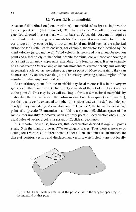
54 Vector calculus on manifolds
3.2 Vector fields on manifolds
A vector field defined on (some region of) a manifold assigns a single vectorto each point P in (that region of) . The vector at P is often drawn as anextended directed line segment with its base at P, but this convention requirescareful interpretation on general manifolds. Once again it is convenient to illustrateour discussion by considering a two-dimensional manifold such as the sphericalsurface of the Earth. Let us consider, for example, the vector field defined by thewind velocity (at ground level). Wind velocity is measured at a given observationpoint and refers solely to that point, despite the visual convenience of showing iton a chart as an arrow apparently extending for a long distance. It is an exampleof a local vector. Other examples include momentum, current density and velocityin general. Such vectors are defined at a given point P. More accurately, they canbe measured by an observer (bug) in a laboratory covering a small region of themanifold in the neighbourhood of P.
At an arbitrary point P in the manifold, any local vector v lies in the tangentspace TP to the manifold at P. Indeed, TP consists of the set of all (local) vectorsat the point P. This may be visualised simply for two-dimensional manifolds byembedding them as surfaces in three-dimensional Euclidean space (see Figure 3.1),but the idea is easily extended to higher dimensions and can be defined indepen-dently of any embedding. As we discussed in Chapter 2, the tangent space at anypoint of a (pseudo-)Riemannian manifold is a (pseudo-)Euclidean space of thesame dimensionality. Moreover, at an arbitrary point P, local vectors obey all theusual rules of vector algebra in (pseudo-)Euclidean geometry.
It is important to realise, however, that local vectors defined at different pointsP and Q in the manifold lie in different tangent spaces. Thus there is no way ofadding local vectors at different points. Other notions that must be abandoned arethose of position vectors and displacement vectors, which clearly are not locally
TPP
Figure 3.1 Local vectors defined at the point P lie in the tangent space TP tothe manifold at that point.
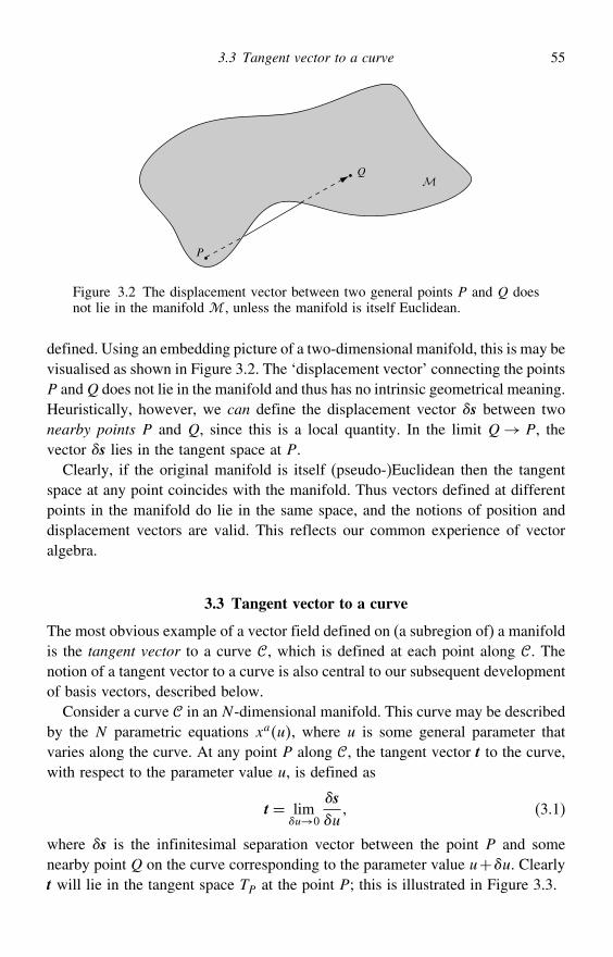
3.3 Tangent vector to a curve 55
P
Q
Figure 3.2 The displacement vector between two general points P and Q doesnot lie in the manifold , unless the manifold is itself Euclidean.
defined. Using an embedding picture of a two-dimensional manifold, this is may bevisualised as shown in Figure 3.2. The ‘displacement vector’ connecting the pointsP andQ does not lie in the manifold and thus has no intrinsic geometrical meaning.Heuristically, however, we can define the displacement vector s between twonearby points P and Q, since this is a local quantity. In the limit Q→ P, thevector s lies in the tangent space at P.
Clearly, if the original manifold is itself (pseudo-)Euclidean then the tangentspace at any point coincides with the manifold. Thus vectors defined at differentpoints in the manifold do lie in the same space, and the notions of position anddisplacement vectors are valid. This reflects our common experience of vectoralgebra.
3.3 Tangent vector to a curve
The most obvious example of a vector field defined on (a subregion of) a manifoldis the tangent vector to a curve , which is defined at each point along . Thenotion of a tangent vector to a curve is also central to our subsequent developmentof basis vectors, described below.
Consider a curve in an N -dimensional manifold. This curve may be describedby the N parametric equations xau, where u is some general parameter thatvaries along the curve. At any point P along , the tangent vector t to the curve,with respect to the parameter value u, is defined as
t = limu→0
su
(3.1)
where s is the infinitesimal separation vector between the point P and somenearby point Q on the curve corresponding to the parameter value u+u. Clearlyt will lie in the tangent space TP at the point P; this is illustrated in Figure 3.3.
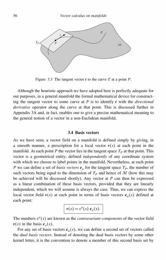
56 Vector calculus on manifolds
TP
P
t
Figure 3.3 The tangent vector t to the curve at a point P.
Although the heuristic approach we have adopted here is perfectly adequate forour purposes, in a general manifold the formal mathematical device for construct-ing the tangent vector to some curve at P is to identify t with the directionalderivative operator along the curve at that point. This is discussed further inAppendix 3A and, in fact, enables one to give a precise mathematical meaning tothe general notion of a vector in a non-Euclidean manifold.
3.4 Basis vectors
As we have seen, a vector field on a manifold is defined simply by giving, ina smooth manner, a prescription for a local vector vx at each point in themanifold. At each point P the vector lies in the tangent space TP at that point. Thisvector is a geometrical entity, defined independently of any coordinate systemwith which we choose to label points in the manifold. Nevertheless, at each pointP we can define a set of basis vectors ea for the tangent space TP , the number ofsuch vectors being equal to the dimension of TP and hence of (how this maybe achieved will be discussed shortly). Any vector at P can then be expressedas a linear combination of these basis vectors, provided that they are linearlyindependent, which we will assume is always the case. Thus, we can express thelocal vector field vx at each point in terms of basis vectors eax defined ateach point:
vx= vax eax
The numbers vax are known as the contravariant components of the vector fieldvx in the basis eax.
For any set of basis vectors eax, we can define a second set of vectors calledthe dual basis vectors. Instead of denoting the dual basis vectors by some otherkernel letter, it is the convention to denote a member of this second basis set by
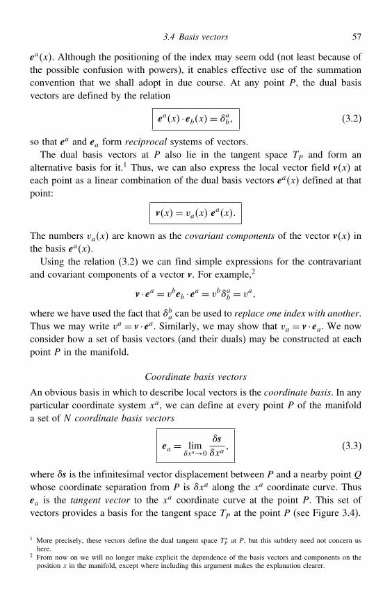
3.4 Basis vectors 57
eax. Although the positioning of the index may seem odd (not least because ofthe possible confusion with powers), it enables effective use of the summationconvention that we shall adopt in due course. At any point P, the dual basisvectors are defined by the relation
eax · ebx= ab (3.2)
so that ea and ea form reciprocal systems of vectors.The dual basis vectors at P also lie in the tangent space TP and form an
alternative basis for it.1 Thus, we can also express the local vector field vx ateach point as a linear combination of the dual basis vectors eax defined at thatpoint:
vx= vax eax
The numbers vax are known as the covariant components of the vector vx inthe basis eax.Using the relation (3.2) we can find simple expressions for the contravariant
and covariant components of a vector v. For example,2
v · ea = vbeb · ea = vbab = va
where we have used the fact that ba can be used to replace one index with another.Thus we may write va = v · ea. Similarly, we may show that va = v · ea. We nowconsider how a set of basis vectors (and their duals) may be constructed at eachpoint P in the manifold.
Coordinate basis vectors
An obvious basis in which to describe local vectors is the coordinate basis. In anyparticular coordinate system xa, we can define at every point P of the manifolda set of N coordinate basis vectors
ea = limxa→0
sxa
(3.3)
where s is the infinitesimal vector displacement between P and a nearby point Qwhose coordinate separation from P is xa along the xa coordinate curve. Thusea is the tangent vector to the xa coordinate curve at the point P. This set ofvectors provides a basis for the tangent space TP at the point P (see Figure 3.4).
1 More precisely, these vectors define the dual tangent space T ∗P at P, but this subtlety need not concern ushere.
2 From now on we will no longer make explicit the dependence of the basis vectors and components on theposition x in the manifold, except where including this argument makes the explanation clearer.
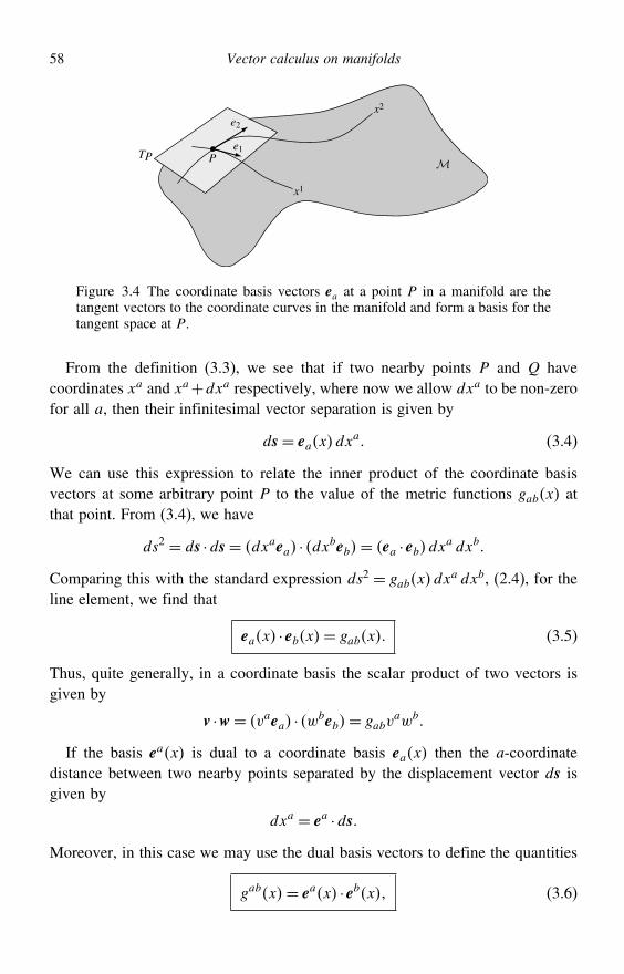
58 Vector calculus on manifolds
x1
x2
TPe1
e2
P
Figure 3.4 The coordinate basis vectors ea at a point P in a manifold are thetangent vectors to the coordinate curves in the manifold and form a basis for thetangent space at P.
From the definition (3.3), we see that if two nearby points P and Q havecoordinates xa and xa+dxa respectively, where now we allow dxa to be non-zerofor all a, then their infinitesimal vector separation is given by
ds= eaxdxa (3.4)
We can use this expression to relate the inner product of the coordinate basisvectors at some arbitrary point P to the value of the metric functions gabx atthat point. From (3.4), we have
ds2 = ds ·ds= dxaea · dxbeb= ea · ebdxa dxbComparing this with the standard expression ds2 = gabxdx
a dxb, (2.4), for theline element, we find that
eax · ebx= gabx (3.5)
Thus, quite generally, in a coordinate basis the scalar product of two vectors isgiven by
v ·w= vaea · wbeb= gabvawb
If the basis eax is dual to a coordinate basis eax then the a-coordinatedistance between two nearby points separated by the displacement vector ds isgiven by
dxa = ea ·dsMoreover, in this case we may use the dual basis vectors to define the quantities
gabx= eax · ebx (3.6)
3.5 Raising and lowering vector indices 59
which, as we will show, form the contravariant components of the metric tensorand are in general different from the quantites gabx; we will return to theselater.
Orthonormal basis vectors at a point
At any given point P in a manifold, it is often useful to define a set of orthonormalbasis vectors ea in TP , which are chosen to be of unit length and orthogonal toone another. This is expressed mathematically by the requirement that at P
ea · eb = ab (3.7)
where ab= diag±1±1 ±1 is the Cartesian line element of the tangentspace TP and depends on the signature of the (in general) pseudo-Riemannianmanifold (see Section 2.13). These orthonormal basis vectors need not be relatedto any particular coordinate system that we are using to label the manifold,although they can always be defined by, for example, giving their componentsin a coordinate basis. Moreover, it is clear from (3.7) that the orthonormal basisvectors ea at P are in fact the coordinate basis vectors of a coordinate system forwhich gabP= ab (or gabP= ab for a strictly Riemannian manifold).
3.5 Raising and lowering vector indices
Unless otherwise stated, we will assume that we are working with a coordinatebasis, as discussed above, and its dual. The contravariant and covariant compo-nents in these bases are equally good ways of specifying a vector. The linkbetween them is found by considering the different ways in which one can writethe scalar product v ·w of two vectors. First, we can write
v ·w= vaea · wbeb= ea · ebvawb = gabvawb
where we have used the contravariant components of the two vectors. Similarly,using the covariant components, we can write the scalar product as
v ·w= vaea · wbe
b= ea · ebvawb = gabvawb
Finally, we could express the scalar product in terms of the contravariant compo-nents of one vector and the covariant components of the other,
v ·w= vaea · wbeb= vawbea · eb= vawb
ba = vawa
similarly, we could write
v ·w= vaea · wbeb= vaw
bea · eb= vawbab = vaw
a
60 Vector calculus on manifolds
By comparing these four alternative expressions for the scalar product of twovectors, we can deduce one of the most useful properties of the quantities gab andgab. Since gabv
awb = vawa holds for any arbitrary vector v, it follows that
gabwb = wa
which illustrates the fact that the quantities gab can be used to lower an index.In other words, we can obtain the covariant components of a vector from itscontravariant components. By a similar argument, we have
gabwb = wa
so that the quantities gab can be used to perform the reverse process of raisingan index. It is straightforward to show that the coordinate and dual basis vectorsthemselves are related in an analogous way by
ea = gabeb and ea = gabeb
We will now prove the useful result that the matrix gab containing thecontravariant components of the metric tensor is the inverse of the matrix gab thatcontains its covariant components. Using the index-lowering and index-raisingaction of gab and gab on the components of an arbitrary vector v, we find that
acvc = va = gabvb = gabgbcv
c
but since v is arbitrary we must have
gabgbc = ac (3.8)
Denoting the matrix gab by G and the matrix gab by G, this equationcan be written in matrix form as GG= I. Hence G and G are inverse matrices.
3.6 Basis vectors and coordinate transformations
Let us consider a coordinate transformation xa → x′a on a manifold. There isa simple relationship between the coordinate basis vectors ea associated withthe coordinate system xa and the coordinate basis vectors e′a associated with thenew system of coordinates x′a. It can be found by considering the infinitesi-mal displacement vector ds between two nearby points P and Q. Clearly, thisdisplacement cannot depend on the coordinate system being used, so we must have
ds= dxaea = dx′ae′a
3.7 Coordinate-independent properties of vectors 61
Noting that dxa = xa/x′b dx′b, we find that at any point P the two sets ofcoordinate basis vectors are related by
e′a =xb
x′aeb (3.9)
where the partial derivative is evaluated at the point P. Repeating this calculationusing the dual basis vectors, we find that
e′a = x′a
xbeb (3.10)
Using (3.9) and (3.10), we can now calculate how the components of anygeneral vector v must transform under the coordinate transformation. Since avector is a geometrical entity that is independent of the coordinate system, wehave (for example)
v= vaea = v′ae′a
So, the new contravariant components are given by
v′a = e′a · v= x′a
xbeb · v ⇒ v′a = x′a
xbvb
Similarly, the new covariant components are given by
v′a = e′a · v=xb
x′beb · v ⇒ v′a =
xb
x′avb
3.7 Coordinate-independent properties of vectors
As we have seen, in a coordinate basis and its dual the scalar product v ·w of twovectors at each point P of the manifold can be written in four ways:
gabvawb = gabvawb = vawa = vaw
a
Using the transformation properties of the metric coefficients gab and those of thevector components, it is straightforward to show that these expressions yield thesame result in any other coordinate system.
In a strictly Riemannian manifold the scalar product is positive definite, whichmeans that gabv
avb ≥ 0 for all vectors va, with gabvavb = 0 only if va = 0. In a
pseudo-Riemannian space, however, this condition is relaxed and leads to somerather odd properties, such as the possibility of non-zero vectors having zero
62 Vector calculus on manifolds
length. We must therefore make definitions that allow us to deal with such prop-erties in a way that extends and generalises familiar concepts in Euclidean space.
The length of a vector v is defined in terms of its components by
gabvavb1/2 = gabvavb1/2 = vava1/2A unit vector has length unity. As remarked above, in a pseudo-Riemannianmanifold we can have vava1/2 = 0 for va = 0, in which case the vector v isdescribed as null.
The angle between two non-null vectors v and w is defined by
cos = vawa
vbvb1/2wcwc1/2
In a pseudo-Riemannian manifold, this formula can lead to cos> 1, resultingin a non-real value for .
Two vectors are orthogonal if their scalar product is zero. This definition makessense even if one or both of the vectors is or are null. In fact, a null vector is anon-zero vector that is orthogonal to itself.
3.8 Derivatives of basis vectors and the affine connection
As we have said, local vectors at different points P and Q in a manifold liein different tangent spaces, so there is no way of adding or subtracting them.In order to define the derivative of a vector field, however, one must comparevectors at different points, albeit in the limit where the distance between the pointstends to zero. We will adopt here an intuitive approach that is sufficient for ourpurposes in developing vector calculus on curved manifolds and provides a simplegeometrical picture. Specifically, on this occasion, we will assume the manifoldto be embedded in a higher-dimensional (pseudo-)Euclidean space, which thusallows vectors at different points to be compared.3
In some arbitrary coordinate system xa on the manifold, let us consider the basisvectors ea at two nearby points P and Q with coordinates xa and xa+xa respec-tively (see Figure 3.5). In general, the basis vectors at Q will differ infinitesimallyfrom those at P, so that
eaQ= eaP+ea
3 It is worth noting that one can embed any four-dimensional torsionless (pseudo-)Riemannian manifold insome (pseudo-)Euclidean space of sufficiently higher dimension; see, for example, J. Nash, The imbeddingproblem for Riemannian manifolds, Annals of Mathematics 63, 20–63, 1956 and C. Clarke, On the globalisometric embedding of pseudo-Riemannian manifolds, Proceedings of the Royal Society A314, 417–28,1970. Indeed, recent theoretical work on braneworld models suggests that our spacetime may indeed beembedded in some higher-dimensional manifold! Alternatively, one can define the derivative of a vector fieldon a general manifold without using an embedding picture, but in a rather more formal manner; see, forexample, R.M. Wald, General Relativity, University of Chicago Press, 1984.
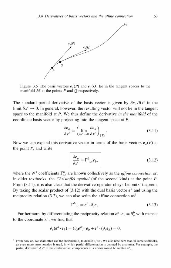
3.8 Derivatives of basis vectors and the affine connection 63
Q
P
ea(Q)ea(P)
Figure 3.5 The basis vectors eaP and eaQ lie in the tangent spaces to themanifold at the points P and Q respectively.
The standard partial derivative of the basis vector is given by ea/xc in the
limit xc→ 0. In general, however, the resulting vector will not lie in the tangentspace to the manifold at P. We thus define the derivative in the manifold of thecoordinate basis vector by projecting into the tangent space at P,
eaxc
≡(
limxc→0
eaxc
)TP
(3.11)
Now we can expand this derivative vector in terms of the basis vectors eaP atthe point P, and write
eaxc
= baceb (3.12)
where the N 3 coefficients bac are known collectively as the affine connection or,
in older textbooks, the Christoffel symbol (of the second kind) at the point P.From (3.11), it is also clear that the derivative operator obeys Leibnitz’ theorem.By taking the scalar product of (3.12) with the dual basis vector ed and using thereciprocity relation (3.2), we can also write the affine connection as4
bac = eb · cea (3.13)
Furthermore, by differentiating the reciprocity relation ea ·eb = ba with respectto the coordinate xc, we find that
cea · eb= ce
a · eb+ ea · ceb= 0
4 From now on, we shall often use the shorthand c to denote /xc. We also note here that, in some textbooks,an even more terse notation is used, in which partial differentation is denoted by a comma. For example, thepartial derivative cv
a of the contravariant components of a vector would be written vac.
64 Vector calculus on manifolds
Then, on using (3.13), we find that the derivatives of the dual basis vectors withrespect to the coordinates are given by
cea =− a
bceb (3.14)
The expressions (3.12–3.14) will be used extensively in our subsequent discus-sions.
3.9 Transformation properties of the affine connection
From the expression (3.13) for the affine connection,
abc = ea · eb
xc (3.15)
we see that, in some new coordinate system x′a, it is given by
′abc = e′a · e′b
x′c
Substituting the expressions (3.9) and (3.10) for the new basis and dual basisvectors, we find
′abc =x′a
xded ·
x′c
(xf
x′bef
)= x′a
xded ·
(xf
x′befx′c
+ 2xf
x′cx′bef
)= x′a
xdxf
x′bxg
x′ced · ef
xg+ x′a
xd2xf
x′cx′bed · ef
= x′a
xdxf
x′bxg
x′c d
fg+x′a
xd2xd
x′cx′b (3.16)
where in the last line we have used the reciprocity relation (3.2) between thebasis and dual basis vectors. We will see later that, because of the presence ofthe last term on the right-hand side of (3.16), the a
bc do not transform as thecomponents of a tensor.
By swapping derivatives with respect to x and x′ in the last term on theright-hand side of (3.16), we arrive at an alternative (but equivalent) expression:
′abc =x′a
xdxf
x′bxg
x′c d
fg−xd
x′bxf
x′c2x′a
xdxf (3.17)
3.10 Relationship of the connection and the metric 65
3.10 Relationship of the connection and the metric
The observant reader will have noticed that there was some arbitrariness in howwe introduced the affine connection in (3.12). We could just as easily have written(3.12) with b
ac replaced by bca, i.e. with the two subscripts interchanged. In
a general Riemannian manifold, these two sets of quantities are not necessarilyequal to one another. In fact, one can show that the quantities
Tbac = b
ac− bca (3.18)
are the components of a third-rank tensor (see Chapter 4) called the torsion tensor.For our considerations of standard general relativity, however, we can assumethat our manifolds are torsionless, so that Tb
ac = 0 in any coordinate system.5
Hence, from here onwards, we will assume (unless otherwise stated) that theaffine connection is symmetric in its last two indices, i.e.
bac = b
ca (3.19)
In a manifold that is torsionless, so that (3.19) is satisfied, there is a simplerelationship between the affine connection b
ac and the metric functions gab,which we now derive. From (3.5) we have gab = ea · eb. Differentiating thisexpression with respect to xc, we obtain
cgab = cea · eb+ ea · ceb= d
aced · eb+ ea · dbced
= dacgdb+ d
bcgad (3.20)
By cyclically permuting the indices ab c, we obtain two equivalent expressions,
bgca = dcbgda+ d
abgcd
agbc = dbagdc+ d
cagbd
Using these three expressions, we now form the combination
cgab+ bgca− agbc
= dacgdb+ d
bcgad+ dcbgda+ d
abgcd− dbagdc− d
cagbd = 2 dcbgad
where, in obtaining the last line, we have used the assumed symmetry properties(3.19) of the affine connection and the symmetry of metric functions. Multiplying
5 It is straightforward to show that any (pseudo-)Riemannian manifold that can be embedded in some (pseudo-)Euclidean space of higher dimension must be torsionless.
66 Vector calculus on manifolds
through by gea, recalling from (3.8) that geagad = ea and relabelling indices, wefinally obtain
abc = 1
2gadbgdc+ cgbd− dgbc (3.21)
In fact, the quantity defined by the right-hand side in (3.21) is properly called themetric connection and is often denoted by the symbol ! a
bc ". In a manifold withtorsion, it will differ from the affine connection defined by (3.11). As we haveshown, however, in a torsionless manifold the affine and metric connections areequivalent, and so a
bc is usually referred to simply as the connection. Unlessotherwise stated, we will follow this convention from now on.
Equation (3.21) is very important, because it tells us how to compute theconnection at any point in a manifold. In other words, if one knows the metric gabin some coordinate system xa then one can form the derivatives of gab appearingin (3.21) and hence calculate all the numbers a
bc at any point.We finish this section by establishing a few useful formulae involving the
connection abc and the related quantities
abc ≡ gad dbc
It is straightforward to show that abc = gad dbc. From (3.21), we find that
abc = 12bgac+ cgba− agbc (3.22)
The quantity abc is traditionally known as a Christoffel symbol of the first kind.Adding bac to abc gives
cgab = abc+ bac (3.23)
which allows us to express partial derivatives of the metric components in termsof the connection coefficients. If we denote the value of the determinant det gabby g then the cofactor of the element gab in this determinant is ggab (note thatg is not a scalar: changing coordinates changes the value of g at any point). Itfollows that cg = ggabcgab, so from (3.23) we have
cg = ggab abc+ bac= g( b
bc+ aac
)= 2g aac (3.24)
The implied summation over a is an example of a contraction over a pair ofindices (see Chapter 4); a
ac means simply 11c+ 2
2c+· · ·+ NNc. Thus the
contraction of the connection coefficients (3.21) is given by
aab = 1
2g−1bg = 1
2b ln g (3.25)
3.11 Local geodesic and Cartesian coordinates 67
the modulus signs being needed if the manifold is pseudo-Riemannian. Alterna-tively, we can write
aab = b ln
√g = 1√g b√g (3.26)
3.11 Local geodesic and Cartesian coordinates
In Chapter 2, we showed that at any point P in a pseudo-Riemannian manifold itis possible in principle to find local Cartesian coordinates x′a such that
g′abP = ab (3.27)
g′abx′c
∣∣∣∣P
= 0 (3.28)
where ab = diag±1±1 ±1. The number of positive entries in ab
minus the number of negative entries is the signature of the manifold. Supposingthat we start with some general system of coordinates xa, we now show how toobtain local Cartesian coordinates in practice.
Let us begin by demanding that our new coordinate system x′a satisfies thecondition (3.28) but not necessarily the condition (3.27). From our expression(3.20) for the derivative of the metric in terms of the connection, we see thatthe condition (3.28) will be satisfied if the connection coefficients in the newcoordinate system vanish at P, i.e.
′abcP= 0 (3.29)
Conversely, from (3.21) we see that the condition (3.28) implies (3.29). Thecondition (3.29) makes much simpler the mathematics of parallel transport, covari-ant differentiation and intrinsic differentiation (see later). Coordinates for which(3.29) holds are generally referred to as geodesic coordinates about P, but this isnot always appropriate since they need not be based on geodesics (which we willalso discuss later).
Suppose that we start with some arbitrary coordinate system xa, the ‘original’system, in which the point P has coordinates xaP . Let us now define a new systemof coordinates x′a by
x′a = xa−xaP+ 12
abcP
(xb−xbP
) (xc−xcP
) (3.30)
68 Vector calculus on manifolds
where the abcP are the connection coefficients at P in the original coordinate
system. Clearly, the origin of the new coordinate system is at P. Differentiationof (3.30) with respect to xd yields
x′a
xd= ad+ a
dcP xc−xcP
so that, at the point P, x′a/xd = ad; its inverse is given by xa/x′d = ad.Differentiating again we obtain
2x′a
xexd= a
dcPce = a
deP
If we now substitute these results into the expression (3.17) for the transformationproperties of the connection, we find that
′abcP= adfb
gc
dfgP−db
fc
adf P= a
bcP− abcP= 0
So in the new (primed) coordinate system the connection coefficients at P arezero, and from (3.29) we have a system of geodesic coordinates at P.
The metric functions g′abP in the geodesic coordinates x′a will not necessarilysatisfy the condition (3.27). Nevertheless, we can obtain such a system of localCartesian coordinates by making a second linear coordinate transformation
x′′a = Xabx′b
where the coefficients Xab are constants. Thus we can bring the metric g′′abP
in these coordinates into the form (3.27) without affecting its derivatives, so that(3.28) will still be satisfied. The required values of the coefficients Xa
b werediscussed in Section 2.13.
3.12 Covariant derivative of a vector
Suppose that a vector field vx is defined over some region of a manifold. Wewill consider the derivative of this vector field with respect to the coordinateslabelling the points in the manifold. Let us begin by writing the vector in termsof its contravariant components v= vaea. We thus obtain
bv= bvaea+vabea (3.31)
where the second term arises because, in an arbitrary coordinate system, the coor-dinate basis vectors vary with the position in the manifold. If we defined locallyCartesian coordinates at some point P in the manifold then in the neighbourhoodof this point the coordinate basis vectors are constant and so the second term wouldvanish at P (but not elsewhere, unless the manifold is (pseudo-)Euclidean, sothat the whole of can be covered by a Cartesian coordinate system).
3.12 Covariant derivative of a vector 69
Using (3.13), we may write (3.31) as
bv= bvaea+va c
abec
Since a and c are dummy indices in the last term on the right-hand side, we mayinterchange them to obtain
bv= bvaea+vc a
cbea = bva+vc a
cb ea
The reason for interchanging the dummy indices is that we may then factor outea. Thus, at any point P, we now have an expression for the derivative of a vectorfield with respect to the coordinates in terms of the basis vectors of the coordinatesystem at P. The quantity in brackets is called the covariant derivative of thevector components, and the standard notation for it is6
bva ≡ bv
a+ acbv
c (3.32)
Thus the derivative of the vector field v can be written in the compact notation
bv= bvaea
We note that, in local geodesic coordinates about some point P, the second termin the covariant derivative (3.32) vanishes at P and thus reduces to the ordinarypartial derivative.
So far we have considered only the covariant derivative of the contravariantcomponents va of a vector. The corresponding result for the covariant componentsva may be found in a similar way, by considering the derivative of v= vae
a andusing (3.14) to obtain
bva = bva− cabvc (3.33)
Comparing the expressions (3.32) and (3.33) for the covariant derivatives ofthe contravariant and covariant components of a vector respectively, we see thatthere are some similarities and some differences. It may help to remember thatthe index with respect to which the covariant derivative is taken (b in this case) isalso the last subscript on the connection; the remaining indices can then only bearranged in one way without raising or lowering them. Finally, the sign differencemust be remembered: for a contravariant index (superscript) the sign is positive,whereas for a covariant index (subscript) the connection carries a minus sign.
We conclude this section by considering the covariant derivative of a scalar.The covariant derivative differs from the simple partial derivative only becausethe coordinate basis vectors change with position in the manifold. However, a
6 In some textbooks, the covariant derivative is denoted by a semicolon, so that the covariant derivative bva
would be written as vab .
70 Vector calculus on manifolds
scalar does not depend on the basis vectors at all, so its covariant derivativemust be the same as its partial derivative, i.e.
b= b (3.34)
3.13 Vector operators in component form
The equations of electromagnetism, fluid mechanics and many other areas ofclassical physics make use of vector calculus in three-dimensional Euclideanspace, employing the gradient and the Laplacian 2 of scalar fields, togetherwith the divergence · v and the curl × v of a vector field. Explicit forms forthese are given in many texts for useful coordinate systems such as Cartesian,cylindrical polar, spherical polar (typically the 11 coordinate systems in whichLaplace’s equation separates). The covariant derivative provides a unified pictureof all these derivatives and a direct route to the explicit forms in an arbitrarycoordinate system. Moreover, it allows for the generalisation of these operatorsto more general manifolds.
Gradient
The gradient of a scalar field is given simply by
= aea = ae
a (3.35)
since the covariant derivative of a scalar is the same as its partial derivative.
Divergence
Replacing the partial derivatives that occur in local Cartesian coordinates bycovariant derivatives, which are valid in arbitrary coordinate systems, the diver-gence of a vector field is given by the scalar quantity
· v= ava = av
a+ aabv
b
Using the result (3.26) we can rewrite the divergence as
· v≡ ava = 1√g a
(√gva) (3.36)
where g is the determinant of the matrix gab.
3.14 Intrinsic derivative of a vector along a curve 71
Laplacian
If we replace v by in · v then we obtain the Laplacian 2. From (3.35),v= vae
a= aea, so the covariant components are va= a. In (3.36), however,
we require the contravariant components va. These may be obtained by raisingthe index with the metric to give
va = gabvb = gabb
Subtituting this into (3.36), we obtain
2≡ aa= 1√g a
(√ggabb) It is worth noting that the symbol used for the Laplacian operator often dependson the dimensionality of the manifold being used. In particular, the triangular(three-sided) symbol 2 that is commonly used in the three-dimensional (andN -dimensional cases) is replaced by the box-shaped (four-sided) symbol 2 infour-dimensional spacetimes, in which case it is called the d’Alembertian operator.
Curl
The special form of the curl of a vector field, which is itself a vector, existsonly in three dimensions. In its more general form, which is valid in higherdimensions, the curl is defined as a rank-2 antisymmetric tensor (see Chapter 4)with components
curl vab = avb−bva
In fact this difference of covariant derivatives can be simplified, since
avb−bva = avb− cbavc− bva+ c
abvc = avb− bva
where the connections have cancelled because of their symmetry properties.
3.14 Intrinsic derivative of a vector along a curve
Normally, we think of vector fields as functions of the coordinates xa definedover some region of the manifold. However, we can also encounter vector fieldsthat are defined only on some subspace of the manifold, and an extreme exampleoccurs when the vector field vu is defined only along some curve xau in themanifold; an example might be the spin 4-vector s of a single particle alongits worldline in spacetime. We now consider how to calculate the derivative ofsuch a vector with respect to the parameter u along the curve.
72 Vector calculus on manifolds
Let us begin by writing the vector field at any point along the curve as
vu= vaueau
where the eau are the coordinate basis vectors at the point on the curve corre-sponding to the parameter value u. Thus, the derivative of v along the curve isgiven by
dvdu= dva
duea+va
deadu
= dva
duea+va
eaxc
dxc
du
where we have used the chain rule to rewrite the last term on the right-hand side;this is a valid procedure since the basis vectors ea are also defined away fromthe curve . Using (3.13) to write the partial derivatives of the basis vectors interms of the connection, we obtain
dvdu= dva
duea+ b
acva dx
c
dueb
Interchanging the dummy indices a and b in the last term, we may factor out thebasis vector, and we find that
dvdu=(dva
du+ a
bcvb dx
c
du
)ea ≡
Dva
Duea (3.37)
The term in parentheses is called the intrinsic (or absolute) derivative of thecomponents va along the curve and is often denoted by Dva/Du as indicated.Similarly, the intrinsic derivative of the covariant components va of a vector isgiven by
DvaDu
= dvadu
− bacvb
dxc
du
A convenient way to remember the form of the intrinsic derivative is to pretendthat the vector v is in fact defined throughout (some region of) the manifold, i.e.not only along the curve . In some cases of interest, this may in fact be trueanyway; for example, v might denote the 4-velocity of some distributed fluid. Wecan now differentiate the components va (say) with respect to the coordinates xa.Thus we can write
dva
du= va
xcdxc
du
Substituting this into (3.37), we can then factor out dxc/du and recognise theother factor as the covariant derivative cv
a. Thus we can write
Dva
Du= cv
adxc
du(3.38)
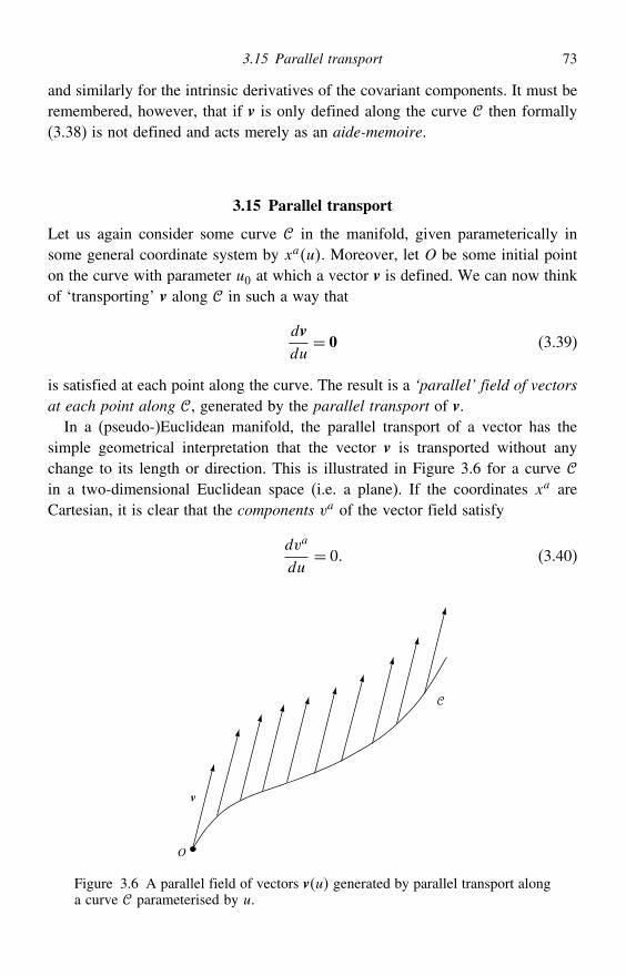
3.15 Parallel transport 73
and similarly for the intrinsic derivatives of the covariant components. It must beremembered, however, that if v is only defined along the curve then formally(3.38) is not defined and acts merely as an aide-memoire.
3.15 Parallel transport
Let us again consider some curve in the manifold, given parameterically insome general coordinate system by xau. Moreover, let O be some initial pointon the curve with parameter u0 at which a vector v is defined. We can now thinkof ‘transporting’ v along in such a way that
dvdu= 0 (3.39)
is satisfied at each point along the curve. The result is a ‘parallel’ field of vectorsat each point along , generated by the parallel transport of v.In a (pseudo-)Euclidean manifold, the parallel transport of a vector has the
simple geometrical interpretation that the vector v is transported without anychange to its length or direction. This is illustrated in Figure 3.6 for a curve in a two-dimensional Euclidean space (i.e. a plane). If the coordinates xa areCartesian, it is clear that the components va of the vector field satisfy
dva
du= 0 (3.40)
O
v
Figure 3.6 A parallel field of vectors vu generated by parallel transport alonga curve parameterised by u.
74 Vector calculus on manifolds
In an arbitrary coordinate system in the plane, however, (3.40) is no longer valid,and from (3.37) we see that it must be generalised to
Dva
Du≡ dva
du+ a
bcvb dx
c
du= 0 (3.41)
From the basic requirement (3.39), it is clear that (3.41) is equally valid for theparallel transport of a vector along a curve in any (pseudo-)Riemannian manifoldin some arbitrary coordinate system xa, although the geometrical interpretation ismore subtle in this case. If one is willing to adopt a picture in which the (pseudo-)Riemannian manifold is embedded in a (pseudo-)Euclidean space of sufficientlyhigher dimension, then one can recover a simple geometrical interpretation ofparallel transport. Consider some curve in the (pseudo-)Riemannian manifoldgiven in terms of some coordinate system in the manifold by xau. Let P andQ be two neighbouring points on the curve with affine parameter values u andu+ u respectively. Starting with the vector v at P, which lies in the tangentspace TP , shift the vector to the neighbouring point Q while keeping it parallelto itself. In a Euclidean embedding space, this simply means transporting thevector without changing its length or direction. At the point Q the vector willnot, in general, lie in the tangent space TQ, on account of the curvature of theembedded manifold. Nevertheless, by considering only that part of the vectorthat is tangential to the embedded manifold at Q, we obtain a definite vectorlying in TQ. It is straightforward to show that this vector coincides with theparallel-transported vector at Q according to (3.41).
If we rewrite (3.41) as
dva
du=− a
bcvb dx
c
du (3.42)
then we can see that, if we specify the components va at some arbitrary pointalong the curve, equation (3.43) fixes the components of va along the entirelength of the curve. If you are worried about whether the transportation is reallyparallel, simply consider an infinitesimal displacement of the vector from somepoint P. For a small displacement we can choose locally Cartesian coordinates atP, in which the s vanish, and so setting the covariant derivative equal to zerodescribes an infinitesimal displacement which keeps the vector parallel (dva = 0).
We note here that, in at least one respect, parallel transport along curves in ageneral (pseudo-)Riemannian manifold is significantly different from that alongcurves in a (pseudo-)Euclidean space, in that it is path dependent: the vectorobtained by transporting a given vector from a point P to a remote point Qdepends on the route taken from P to Q. This path dependence is also apparentin transporting a vector around a closed loop, where on returning to the starting
3.16 Null curves, non-null curves and affine parameters 75
point the direction of the transported vector is (in general) different from thevector’s initial direction. This path dependence can be demonstrated on a curvedtwo-dimensional surface, and in general can be expressed mathematically in termsof the curvature tensor of the manifold. We will return to this topic in Chapter 7.
3.16 Null curves, non-null curves and affine parameters
So far, we have treated all curves in a manifold on a equal footing. In pseudo-Riemannian manifolds, however, it is important to distinguish between null curvesand non-null curves. In the former, the interval ds between any two nearby pointson the curve is zero, whereas in the latter case ds is non-zero. The distinctionbetween these two types of curve may also be defined in terms of their tangentvectors, and this leads to the identification of a class of privileged parameters,called affine parameters, in terms of which the curves may be defined.
Consider some curve xau in a general manifold. As discussed earlier, thetangent vector t to the curve at some point P, with respect to the parameter valueu, is defined by (3.1). In a given coordinate system, we can write s = eax
a,where the ea are coordinate basis vectors at P. We then obtain
t = dxa
duea (3.43)
From this expression, we see that the length of the tangent vector t to the curvexau at the point P is given by
t = gabtatb1/2 =∣∣∣∣gab dxadu
dxb
du
∣∣∣∣1/2 = gab dxadxb1/2du
=∣∣∣∣ dsdu
∣∣∣∣ where ds is the distance measured along the curve at P that corresponds to theparameter interval du along the curve.
A non-null curve is one for which the tangent vector at every point is not null,i.e. t = 0. For such a curve, the length of the tangent vector at each point dependson the parameter u and, in general, can vary along the curve. However, we seethat if the curve is parameterised in terms of a parameter u that is related to thedistance s measured along the curve by u= as+b, where a and b are constants,with a = 0, then the length of the tangent vector will be constant along the curve.In this case u is called an affine parameter along the curve. Moreover, if we takeu= s then the tangent vector (with components dxa/ds) is always of unit length.
A null curve is one for which the tangent vector is null, t = 0, at every pointalong the curve; equivalently, the distance ds between any two points on a nullcurve is zero. Since s does not vary along the curve, we clearly cannot use it as
76 Vector calculus on manifolds
a parameter. We are, however, free to use any other non-zero scalar parameter uthat does vary along the curve. Moreover, even for null curves it is still possibleto define a privileged family of affine parameters. The definition of an affineparameter for a null curve is best introduced through the study of geodesics.
3.17 Geodesics
A geodesic in Euclidean space is a straight line, which has two equivalent definingproperties. First, its tangent vector always points in the same direction (alongthe line) and, second, it is the curve of shortest length between two points. Wecan use generalisations of either property to define geodesics in more generalmanifolds. The fixed direction of their tangent vectors can be used to define bothnon-null and null geodesics in a pseudo-Riemannian manifold, whereas clearlythe extremal length can only be used to define non-null geodesics. In a manifoldthat is torsionless (so that (3.19) is satisfied) these two defining properties areequivalent, for non-null geodesics, and lead to the same curves.7
Let us begin by characterising a geodesic as a curve xau described in termsof some general parameter u by the fixed direction of its tangent vector tu. Theequations satisfied by the functions xau are thus determined by the requirementthat, along the curve,
dtdu= u t (3.44)
where u is some function of u. From (3.41), we see that the components ta ofthe tangent vector in the coordinate basis must satisfy
Dta
Du= dta
du+ a
bctb dx
c
du= uta
Since the components of the tangent vector are ta = dxa/du we find that theequations satisfied by a geodesic are
d2xa
du2+ a
bc
dxb
du
dxc
du= u
dxa
du (3.45)
Equation (3.45) is valid for both null and non-null geodesics parameterisedin terms of some general parameter u. If the curve is parameterised in such away that u vanishes, however, then u is a privileged parameter called anaffine parameter. From (3.44), we see that this corresponds to a parameterisation
7 In a manifold with torsion, the two properties lead to different curves: a curve whose length is stationary withrespect to small variations in the path is called a metric geodesic, whereas a curve whose tangent vector isconstant along the path is an affine geodesic.
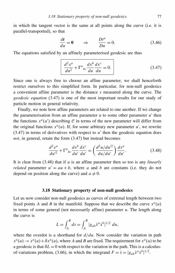
3.18 Stationary property of non-null geodesics 77
in which the tangent vector is the same at all points along the curve (i.e. it isparallel-transported), so that
dtdu= 0 ⇒ Dta
Du= 0 (3.46)
The equations satisfied by an affinely parameterised geodesic are thus
d2xa
du2+ a
bc
dxb
du
dxc
du= 0 (3.47)
Since one is always free to choose an affine parameter, we shall henceforthrestrict ourselves to this simplified form. In particular, for non-null geodesicsa convenient affine parameter is the distance s measured along the curve. Thegeodesic equation (3.47) is one of the most important results for our study ofparticle motion in general relativity.
Finally, we note how affine parameters are related to one another. If we changethe parameterisation from an affine parameter u to some other parameter u′ thenthe functions xau′ describing in terms of the new parameter will differ fromthe original functions xau. If, for some arbitrary new parameter u′, we rewrite(3.47) in terms of derivatives with respect to u′ then the geodesic equation doesnot, in general, retain the form (3.47) but instead becomes
d2xa
du′2+ a
bc
dxb
du′dxc
du′=(d2u/du′2
du/du′
)dxa
du′ (3.48)
It is clear from (3.48) that if u is an affine parameter then so too is any linearlyrelated parameter u′ = au+ b, where a and b are constants (i.e. they do notdepend on position along the curve) and a = 0.
3.18 Stationary property of non-null geodesics
Let us now consider non-null geodesics as curves of extremal length between twofixed points A and B in the manifold. Suppose that we describe the curve xauin terms of some general (not necessarily affine) parameter u. The length alongthe curve is
L=∫ B
Ads =
∫ B
Agabxaxb1/2 du
where the overdot is a shorthand for d/du. Now consider the variation in pathxau→ xau+xau, where A and B are fixed. The requirement for xau to bea geodesic is that L= 0 with respect to the variation in the path. This is a calculus-of-variations problem, (3.66), in which the integrand F = s = gabxaxb1/2.
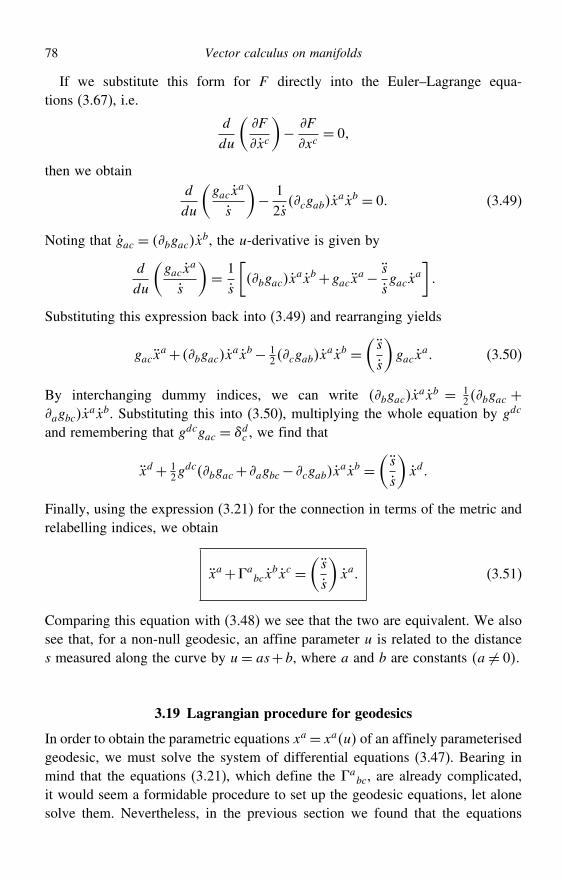
78 Vector calculus on manifolds
If we substitute this form for F directly into the Euler–Lagrange equa-tions (3.67), i.e.
d
du
(F
xc
)− F
xc= 0
then we obtaind
du
(gacx
a
s
)− 1
2scgabx
axb = 0 (3.49)
Noting that gac = bgacxb, the u-derivative is given by
d
du
(gacx
a
s
)= 1
s
[bgacx
axb+gacxa− s
sgacx
a
]
Substituting this expression back into (3.49) and rearranging yields
gacxa+ bgacx
axb− 12cgabx
axb =(s
s
)gacx
a (3.50)
By interchanging dummy indices, we can write bgacxaxb = 1
2bgac +agbcx
axb. Substituting this into (3.50), multiplying the whole equation by gdc
and remembering that gdcgac = dc , we find that
xd+ 12g
dcbgac+ agbc− cgabxaxb =
(s
s
)xd
Finally, using the expression (3.21) for the connection in terms of the metric andrelabelling indices, we obtain
xa+ abcx
bxc =(s
s
)xa (3.51)
Comparing this equation with (3.48) we see that the two are equivalent. We alsosee that, for a non-null geodesic, an affine parameter u is related to the distances measured along the curve by u= as+b, where a and b are constants a = 0.
3.19 Lagrangian procedure for geodesics
In order to obtain the parametric equations xa= xau of an affinely parameterisedgeodesic, we must solve the system of differential equations (3.47). Bearing inmind that the equations (3.21), which define the a
bc, are already complicated,it would seem a formidable procedure to set up the geodesic equations, let alonesolve them. Nevertheless, in the previous section we found that the equations
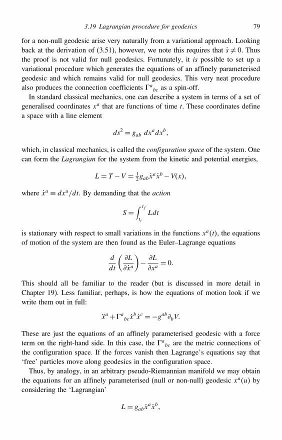
3.19 Lagrangian procedure for geodesics 79
for a non-null geodesic arise very naturally from a variational approach. Lookingback at the derivation of (3.51), however, we note this requires that s = 0. Thusthe proof is not valid for null geodesics. Fortunately, it is possible to set up avariational procedure which generates the equations of an affinely parameterisedgeodesic and which remains valid for null geodesics. This very neat procedurealso produces the connection coefficients a
bc as a spin-off.In standard classical mechanics, one can describe a system in terms of a set of
generalised coordinates xa that are functions of time t. These coordinates definea space with a line element
ds2 = gab dxadxb
which, in classical mechanics, is called the configuration space of the system. Onecan form the Lagrangian for the system from the kinetic and potential energies,
L= T −V = 12gabx
axb−Vx
where xa ≡ dxa/dt. By demanding that the action
S =∫ tf
ti
Ldt
is stationary with respect to small variations in the functions xat, the equationsof motion of the system are then found as the Euler–Lagrange equations
d
dt
(L
xa
)− L
xa= 0
This should all be familiar to the reader (but is discussed in more detail inChapter 19). Less familiar, perhaps, is how the equations of motion look if wewrite them out in full:
xa+ abcx
bxc =−gabbV
These are just the equations of an affinely parameterised geodesic with a forceterm on the right-hand side. In this case, the a
bc are the metric connections ofthe configuration space. If the forces vanish then Lagrange’s equations say that‘free’ particles move along geodesics in the configuration space.
Thus, by analogy, in an arbitrary pseudo-Riemannian manifold we may obtainthe equations for an affinely parameterised (null or non-null) geodesic xau byconsidering the ‘Lagrangian’
L= gabxaxb
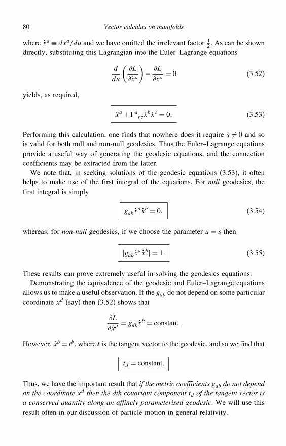
80 Vector calculus on manifolds
where xa ≡ dxa/du and we have omitted the irrelevant factor 12 . As can be shown
directly, substituting this Lagrangian into the Euler–Lagrange equations
d
du
(L
xa
)− L
xa= 0 (3.52)
yields, as required,
xa+ abcx
bxc = 0 (3.53)
Performing this calculation, one finds that nowhere does it require s = 0 and sois valid for both null and non-null geodesics. Thus the Euler–Lagrange equationsprovide a useful way of generating the geodesic equations, and the connectioncoefficients may be extracted from the latter.
We note that, in seeking solutions of the geodesic equations (3.53), it oftenhelps to make use of the first integral of the equations. For null geodesics, thefirst integral is simply
gabxaxb = 0 (3.54)
whereas, for non-null geodesics, if we choose the parameter u= s then
gabxaxb = 1 (3.55)
These results can prove extremely useful in solving the geodesics equations.Demonstrating the equivalence of the geodesic and Euler–Lagrange equations
allows us to make a useful observation. If the gab do not depend on some particularcoordinate xd (say) then (3.52) shows that
L
xd= gdbx
b = constant
However, xb = tb, where t is the tangent vector to the geodesic, and so we find that
td = constant
Thus, we have the important result that if the metric coefficients gab do not dependon the coordinate xd then the dth covariant component td of the tangent vector isa conserved quantity along an affinely parameterised geodesic. We will use thisresult often in our discussion of particle motion in general relativity.
Appendix 3A: Vectors as directional derivatives 81
3.20 Alternative form of the geodesic equations
The most common form of the geodesic equations is that given in (3.53). It issometimes useful, however, to recast the geodesic equations in different forms.Thus, we note here an alternative way of writing them that will be of particularpractical use when we come to study particle motion in general relativity.
From (3.46), for a geodesic we have dt/du = 0. In some coordinate systemwe may write this equation in terms of the intrinsic derivative of the covariantcomponents of the tangent vector as
DtaDu
≡ dtadu
− bactb
dxc
du= 0
Remembering that tc = xc = dxc/du, we thus have
ta = bactbt
c
which, on rewriting the connection coefficients bac using (3.21), becomes
ta = 12g
bdagdc+ cgad− dgactbtc = 1
2agdc+ cgad− dgactdtc
Using the symmetry of the metric tensor, we see that the last two terms in thesummation on d and c cancel. Thus, we obtain a useful alternative form of thegeodesic equations,
ta = 12agcdt
ctd (3.56)
From this equation, we may immediately verify our earlier finding that if themetric gcd does not depend on the coordinate xa then ta = constant.
Appendix 3A: Vectors as directional derivatives
In an arbitrary manifold, the formal mathematical definition of a tangent vectorto a curve at some point P is in terms of the directional derivative along thecurve at that point. In particular, let us consider some curve defined in terms ofan arbitrary coordinate system by xau. In addition, suppose that some arbitraryscalar function fxa is defined on the manifold. At any point P on the curve, thedirectional derivative of f is defined simply as
df
du= f
xadxa
du
at that point. However, ta ≡ dxa/du gives the components of a tangent vector tothe curve at P and, since f is arbitrary, we may write
d
du= ta
xa
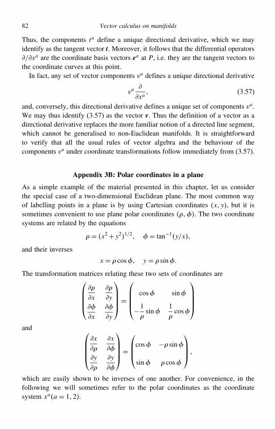
82 Vector calculus on manifolds
Thus, the components ta define a unique directional derivative, which we mayidentify as the tangent vector t. Moreover, it follows that the differential operators/xa are the coordinate basis vectors ea at P, i.e. they are the tangent vectors tothe coordinate curves at this point.
In fact, any set of vector components va defines a unique directional derivative
va
xa (3.57)
and, conversely, this directional derivative defines a unique set of components va.We may thus identify (3.57) as the vector v. Thus the definition of a vector as adirectional derivative replaces the more familiar notion of a directed line segment,which cannot be generalised to non-Euclidean manifolds. It is straightforwardto verify that all the usual rules of vector algebra and the behaviour of thecomponents va under coordinate transformations follow immediately from (3.57).
Appendix 3B: Polar coordinates in a plane
As a simple example of the material presented in this chapter, let us considerthe special case of a two-dimensional Euclidean plane. The most common wayof labelling points in a plane is by using Cartesian coordinates x y, but it issometimes convenient to use plane polar coordinates . The two coordinatesystems are related by the equations
= x2+y21/2 = tan−1y/x
and their inverses
x = cos y = sin
The transformation matrices relating these two sets of coordinates are⎛⎜⎜⎜⎝
x
y
x
y
⎞⎟⎟⎟⎠=⎛⎜⎜⎜⎝ cos sin
−1sin
1cos
⎞⎟⎟⎟⎠and ⎛⎜⎜⎜⎝
x
x
y
y
⎞⎟⎟⎟⎠=⎛⎜⎜⎝cos − sin
sin cos
⎞⎟⎟⎠
which are easily shown to be inverses of one another. For convenience, in thefollowing we will sometimes refer to the polar coordinates as the coordinatesystem xaa= 12.
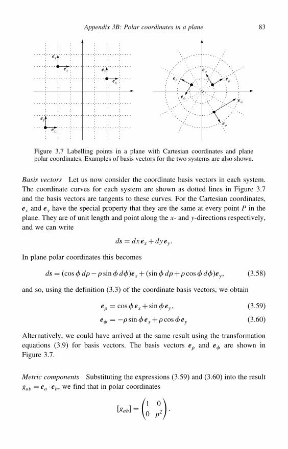
Appendix 3B: Polar coordinates in a plane 83
ex
ey
ex
ex
eρ
eφ
ey
ey
eφ
eρ
eρ
eφ
Figure 3.7 Labelling points in a plane with Cartesian coordinates and planepolar coordinates. Examples of basis vectors for the two systems are also shown.
Basis vectors Let us now consider the coordinate basis vectors in each system.The coordinate curves for each system are shown as dotted lines in Figure 3.7and the basis vectors are tangents to these curves. For the Cartesian coordinates,ex and ey have the special property that they are the same at every point P in theplane. They are of unit length and point along the x- and y-directions respectively,and we can write
ds= dx ex+dy ey
In plane polar coordinates this becomes
ds= cosd− sindex+ sind+ cosdey (3.58)
and so, using the definition (3.3) of the coordinate basis vectors, we obtain
e = cos ex+ sin ey (3.59)
e = − sin ex+ cos ey (3.60)
Alternatively, we could have arrived at the same result using the transformationequations (3.9) for basis vectors. The basis vectors e and e are shown inFigure 3.7.
Metric components Substituting the expressions (3.59) and (3.60) into the resultgab = ea · eb, we find that in polar coordinates
gab=(1 00 2
)
84 Vector calculus on manifolds
Thus, we have
ds2 = ds ·ds= gab dxa dxb = d2+2 d2
which matches the result obtained using (3.58) directly. The matrix gab is theinverse of the matrix gab and thus is given by
gab=(1 00 1/2
)
Dual basis The dual basis vectors given by ea = gabeb are
e = ge+ge = e
e = ge+ge =12
e
where no summation is implied over or . These dual basis vectors are easilyshown to obey the reciprocity relation ea · eb = ab .
Derivatives of basis vectors Since ex and ey are constant vector fields, thederivatives of the polar coordinate basis vectors are easily found as
e
=
cos ex+ sin ey= 0
e
=
cos ex+ sin ey=− sin ex+ cos ey =
1e
These have a simple geometrical picture. At each of two nearby points P andQ the vector e must point away from the origin, and so in slightly differentdirections. The derivative of e with respect to is just the difference betweenbetween e at P and Q divided by (the angle between them). The differencein this case is clearly a vector parallel to e, which makes the above resultsreasonable. Similarly,
e
=
− sin ex+ cos ey=− sin ex+ cos ey =
1e
e
=
− sin ex+ cos ey=− cos ex− sin ey =− e
The student is encouraged to explain these formulae geometrically.
Appendix 3B: Polar coordinates in a plane 85
Connection coefficients Using the general formula cea = baceb, we can now
read off the connection coefficients in plane polar coordinates:
e
=0 ⇒ = 0
= 0
e
= 1e ⇒
= 0 =
1
e
= 1e ⇒
= 0 =
1
e
= − e ⇒ =−
= 0
where no summation is assumed over repeated indices. Thus, although wecomputed the derivatives of e and e by using the constancy of ex and ey, theCartesian basis vectors do not appear in the above equations. The connection’simportance is that it enables one to express these derivatives without usingany other coordinates than polar. We can alternatively calculate the connectioncoefficients from the metric using the general result (3.21). For example,
= 1
2gaga+ ga− ag
where summation is implied only over the index a. Since g= 0 and g= 1/2,we have
=
122
g+ g− g=122
g =122
2= 1
This is the same expression for as that derived above. Indeed, this method of
computing the connection is generally far more straightforward than calculatingthe derivatives of basis vectors.
Covariant derivative Given the connection coefficients, we can calculate thecovariant derivative of a vector field in polar coordinates. As an example of itsuse, let us find an expression for the divergence · v of a vector field. This isgiven by
· v= ava = av
a+ abav
b
Now, the contracted connection coefficients are given by
aa =
+ =
1
aa =
+ = 0
86 Vector calculus on manifolds
so we have
· v= v
+ 1v+ v
= 1
v+ v
This formula may not be immediately familiar. The reason for this is that mostoften a vector v is expressed in terms of the normalised basis vectors e = eand e = e/. In this normalised basis the vector components are v = v andv = v, and the divergence takes its more usual form
· v= 1
v+ 1
v
Geodesics Finally, let us consider a geodesic in a plane. We already know thatthe answer is a straight line, and this is trivially proven in Cartesian coordinates.For illustration, however, let us perform the calculation the hard way, i.e. in planepolar coordinates. There are two geodesic equations,
d2xa
ds2+ a
bc
dxb
ds
dxc
ds= 0
for a = , where we are using the arclength s as our parameter along thegeodesic. The only non-zero connection coefficients are
=− and =
= 1/. Thus, writing out the geodesic equations for a = and a = ,
we have
d2
ds2−
(d
ds
)2
= 0 (3.61)
d2
ds2+ 2
d
ds
d
ds= 0 (3.62)
Also, since in a Euclidean plane we can only have non-null geodesics, a firstintegral of these equations is provided by
gabdxa
ds
dxb
ds= 1 ⇒
(d
ds
)2
+2(d
ds
)2
= 1 (3.63)
Of course, this could have been obtained simply by dividing through ds2 =d2+2 d2 by ds2.
Equation (3.62) can be written as
12
d
ds
(2
d
ds
)= 0
from which we obtain
2d
ds= k= constant (3.64)
Appendix 3C: Calculus of variations 87
Inserting this into (3.63), we find that
d
ds=(1− k2
2
)1/2
(3.65)
The shape of the geodesic is what really interests us, i.e. as a function of orvice versa. Dividing (3.64) by (3.65), we obtain
d
d= k
2
(1− k2
2
)−1/2
which can be integrated easily to give
= 0+ cos−1(k
)
where 0 is the integration constant. The shape of the geodesic is given by
cos−0= k
which, on expanding the cosine and using x = cos and y = sin, gives
x cos0+y sin0 = k
This is the general equation of a straight line. Thus we recover the familiar resultin an unfamiliar coordinate system.
Appendix 3C: Calculus of variations
The calculus of variations provides a means of finding a function (or set offunctions) that makes an integral dependent on the function(s) stationary, i.e.makes the value of the integral a local maximum or minimum. Let us considerthe path integral
I =∫ B
AFxa xa udu (3.66)
where A, B and the form of the integrand F are fixed, but the ‘curve’ or pathxau has to be chosen so as to make stationary the value of I . From (3.66),we see that we are considering quite a general case, in which the integrandF is a function of the 2N independent functions xa and xa ≡ dxa/du and theparameter u.
Now consider making an arbitrary variation xau→ xau+ xau in thepath, keeping the endpoints A and B fixed. The corresponding first-order variationin the value of the integral is
I =∫ B
AF du=
∫ B
A
(F
xaxa+ F
xaxa
)du
88 Vector calculus on manifolds
Integrating the last term by parts and requiring the variation I to be zero, weobtain
I =[F
xaxa
]BA
+∫ B
A
[F
xa− d
du
(F
xa
)]xa du= 0
Since A and B are fixed, the first term vanishes. Then, since xa is arbitrary, ourrequired extremal curve xau must satisfy the N equations
d
du
(F
xa
)− F
xa= 0 (3.67)
These are the Euler–Lagrange equations for the problem.
Exercises
3.1 Show that, in general, ea = gabeb and ea = gabeb. Show also that, under a coordinate
transformation,
e′a =xb
x′aeb and e′a = x′a
xbeb
3.2 Calculate the coordinate basis vectors e′a of the coordinates system x′a in Exercise 2.3in terms of the coordinate basis vectors ea of the Cartesian system. Hence verifythat the metric functions g′ab agree with those found earlier. Calculate the dual basisvectors e′a in the primed system and hence the quantities g′ab. Find the contravariantand covariant components of e1 in the primed basis. Hence verify that e1 is of unitlength.
3.3 For any metric gab show that gabgab = N , where N is the dimension of the manifold.3.4 Show that the affine connection can be written as b
ac = eb ·cea. Show further that,in a torsionless manifold, cea = aec.
3.5 Show that, under a coordinate transformation, the affine connection transforms as
′abc =x′a
xdxf
x′bxg
x′c d
fg−xd
x′bxf
x′c2x′a
xdxf
3.6 For a diagonal metric gab, show that the connection coefficients are given by (witha = b = c and no summation over repeated indices)
abc = 0 b
aa =−1
2gbbbgaa
aba = a
ab = b
(ln√gaa) a
aa = a
(ln√gaa)
3.7 Let g be the determinant of the matrix gab. By considering the cofactor of theelement gab in this determinant, or otherwise, show that cg = ggabcgab.
Exercises 89
3.8 In a manifold with non-zero torsion, show that the affine connection defined by(3.11) may be written as
abc =
a
bc
− 1
2Ta
cb+Tcab−Tbc
a
where
a
bc
is the metric connection defined by the right-hand side of (3.21) and Ta
bc
is the torsion tensor defined in (3.18). Defining an index symmetrisation operationsuch that a
bc ≡ 12
abc+ a
cb, show further that
abc =
a
bc
+Tbc
a
3.9 In a manifold with non-zero torsion, show that the condition abc = 0 implies that
agbc = 0 but not vice versa. Show further that, under a coordinate transformationof the form
x′a = xa−xaP+12 a
bcPxb−xbPx
c−xcP
the affine connection at the point P in the new coordinate system is given by
′abcP=12T ′abcP
and hence the transformation does not yield a set of geodesic coordinates. Is it stillpossible to define local Cartesian coordinates in a manifold with non-zero torsion?
3.10 Show that, for the covariant components va of a vector, the covariant derivative andthe intrinsic derivative along a curve are given respectively by
bva = bva− cabvc and
DvaDu
= dvadu
− bacvb
dxc
du
3.11 Show that for a vector field with contravariant components vb to have a vanishingcovariant derivative av
b everywhere in a manifold, it must satisfy the relation
b dac− c
dab+ e
ac deb− e
ab decv
a = 0
Hint: Use the fact that partial derivatives commute.3.12 If a vector field va vanishes on a hypersurface S that bounds a region V of an
N -dimensional manifold, show that∫Vav
a√−g dNx = 0
3.13 On the surface of a unit sphere, ds2 = d2+ sin2 d2. Calculate the connectioncoefficients in the coordinate system. A vector v of unit length is definedat the point 00 as parallel to the circle = 0. Calculate the components of vafter it has been parallel-transported around the circle = 0. Hence show that,in general, after parallel transport the direction of v is different but its length isunchanged.
90 Vector calculus on manifolds
3.14 If the two vectors with contravariant components va and wa are each parallel-transported along a curve, show that vawa remains constant along the curve. Henceshow that if a geodesic is timelike (or null or spacelike) at some point, it is timelike(or null or spacelike) at all points.
3.15 An affinely parameterised geodesic xau satisfies
d2xa
du2+ a
bc
dxb
du
dxc
du= 0
Show that the form of this equation remains unchanged by an arbitrary coordinatetransformation xa → x′a. Find the form of the geodesic equation for a geodesicdescribed in terms of some general (non-affine) parameter . Hence show that allaffine parameters are related by a linear transformation with constant coefficients.
3.16 If x is an affinely parameterised geodesic, show that
Du
D= 0
where u = dx/d. Hence show that the geodesic equations can be written as
du
d= 1
2g#u
u#
3.17 By substituting the ‘Lagrangian’ L = gabxaxb into the Euler–Lagrange equations,
show directly that
xa+ abcx
bxc = 0
where the dots denote differentiation with respect to an affine parameter.3.18 By transforming from a local inertial coordinate system in which
ds2 = c2d2 = d d
to a general coordinate system x, show that freely falling particles obey the geodesicequations of motion
d2x
d2+
dx
d
dx
d= 0
where
=
x
2
xx
3.19 By considering the ‘Lagrangian’ L = gabxaxb, derive the equations for an affinely
parameterised geodesic on the surface of a sphere in the coordinates . Henceshow that, of all the circles of constant latitude on a sphere, only the equator is ageodesic. Use your geodesic equations to pick out the connection coefficients inthis coordinate system.
3.20 In the 2-space with line element
ds2 = dr2+ r2d2
r2−a2− r2dr2
r2−a22
Exercises 91
where r > a, show that the differential equation for the geodesics may be written as
a2
(dr
d
)2
+a2r2 = Kr4
where K is a constant such that K = 1 if the geodesic is null. By setting r d/dr =tan, show that the space is mapped onto a Euclidean plane in which r aretaken as polar coordinates and the geodesics are mapped to straight lines.
4
Tensor calculus on manifolds
The coordinates with which one labels points in a manifold are entirely arbitrary.For example, we could choose to parameterise the surface of a sphere in termsof the coordinates , taking any point as the north pole, or we could useany number of alternative coordinate systems. It is also clear, however, that ourdescription of any physical processes occurring on the surface of the sphere shouldnot depend on our chosen coordinate system. For example, at any point P on thesurface one can say that, for example, the air temperature has a particular valueor that the wind has a certain speed in a particular direction. These respectivelyscalar and vector physical quantities do not depend on which coordinates are usedto label points in the surface. Thus in, order to describe these physical fieldson the surface, we must formulate our equations in a way that is valid in allcoordinate systems. We have already dealt with such a description for scalar andvector quantities on manifolds, but now we turn to the generalisation of theseideas to quantities that cannot be described as a scalar or a vector. This requiresthe introduction of the concept of tensors.
4.1 Tensor fields on manifolds
Let us begin by considering vector fields in a slightly different manner. Supposewe have some arbitrary vector field, defining a vector t at each point of a manifold.How can we obtain from t a scalar field? Clearly, the only way to do this is totake the scalar product of t with a vector v from another vector field. Thus, ateach point P in the manifold, we can think of vector t in TP as a linear functiont· that takes another vector in TP as its argument and produces a real number.We can denote the number produced by the action of t on a particular vector v by
tv≡ t · v (4.1)
92
4.2 Components of tensors 93
It is now clear how we can generalise the notion of a vector: in the tangentspace TP , we can define a tensor t as a linear map from some number of vectorsto the real numbers. The rank of the tensor is the number of vectors it has for itsarguments. For example, we can write a third-rank tensor as t· · ·. Once again,we denote the number that the tensor t produces from the vectors u, v and w by
tu vw
The tensor is defined by the precise set of operations applied to the vectors u, vand w to produce a scalar. Notice, however, that the definition of a tensor doesnot mention the components of the vectors; a tensor must give the same realnumber independently of the reference system in which the vector componentsare calculated. If at each point P in some region of the manifold we have a tensordefined then the result is a tensor field in this region.
In fact we have already encountered examples of tensors. Clearly, from ourabove discussion, any vector is a rank-1 tensor. Higher-rank tensors thus constitutea generalisation of the concept of a vector. For example, a particularly importantsecond-rank tensor is the metric tensor g, which we have already met. This definesa linear map of two vectors into the number that is their inner product, i.e.
gu v≡ u · v
We will investigate the properties of this special tensor shortly. Finally, we notealso that a scalar function of position x is a real-valued function of no vectorsat all, and is therefore classified as a zero-rank tensor.
The fact that a tensor is a linear map of the vectors into the reals is particularlyuseful. For simplicity, let us consider a rank-1 tensor. Linearity means that, forgeneral vectors u and v and general scalars and ,
tu+v= tu+tv
Similar expansions may be performed for tensors of higher rank. For a second-ranktensor, for example, we can write
tu+v w+ z = tu w+ z+tv w+ z
= tuw+tu z+tvw+tv z
4.2 Components of tensors
When a tensor is evaluated with combinations of basis and dual basis vectorsit yields its components in that particular basis. For example, the covariant and
94 Tensor calculus on manifolds
contravariant components of the rank-1 tensor (vector) in (4.1) in the basis ea aregiven by
tea= ta and tea= ta
Consider now a second-rank tensor t· ·. Its covariant and contravariant compo-nents are given by
tea eb= tab and tea eb= tab
For tensors of rank 2 and higher, however, we can also define sets of mixedcomponents. For a rank-2 tensor there are two possible sets of mixed components,
tea eb= tab and tea eb= ta
b
For a general rank-2 tensor these two sets of components need not be equal.The contravariant, covariant and mixed components of higher-rank tensors can beobtained in an analogous manner.
The components of a tensor in a particular basis set specify the action of thetensor on any other vectors in terms of their components. For example, using thelinearity property, we find that
tu v= tuaea vbeb= tabu
avb
To obtain this result, we expressed u and v in terms of their contravariant compo-nents. We could have written either vector in terms of its contravariant or covariantcomponents, however. Hence we find that there are numerous equivalent expres-sions for tu v in component notation:
tu v= tabuavb = tabuavb = ta
buavb = tabuavb
This illustrates the general rule that the subscript and superscript positions of adummy index can be swapped without affecting the result.
4.3 Symmetries of tensors
A second-rank tensor t is called symmetric or antisymmetric if, for all pairs ofvectors u and v,
tu v=±tvu
4.3 Symmetries of tensors 95
with the plus sign for a symmetric tensor and the minus sign for an antisym-metric tensor. Setting u = ea and v = eb, we see that the covariant componentsof a symmetric or antisymmetric tensor satisfy tab = ±tba. By using differentcombinations of basis and dual basis vectors we also see that, for such a tensor,tab =±tba and ta
b =±tba.An arbitrary rank-2 tensor can always be split uniquely into the sum of its
symmetric and antisymmetric parts. For illustration let us work with the covariantcomponents tab of the tensor in some basis. We can always write
tab = 12tab+ tba+ 1
2tab− tba
which is clearly the sum of a symmetric and an antisymmetric part. A notationfrequently used to denote the components of the symmetric and antisymmetricparts is
tab ≡ 12tab+ tba and t ab ≡ 1
2tab− tba
In an analogous manner, a general rank-N tensor tu v w is symmetricor antisymmetric with respect to some permutation of its vector arguments ifits value after permuting the arguments is equal to respectively plus or minusits original value. From an arbitrary rank-N tensor, however, we can alwaysobtain a tensor that is symmetric with respect to all permutations of its vectorarguments and one that is antisymmetric with respect to all permutations. In termsof the tensor’s covariant components, these symmetric and antisymmetric parts aregiven by
tabc =1N !sum over all permutations of the indices ab c
t abc =1N !alternating sum over all permutations of the indices ab c
For example, the covariant components of the totally antisymmetric part of athird-rank tensor are given by
t abc = 16tabc− tacb+ tcab− tcba+ tbca− tbac
We may extend the notation still further in order to define tensors that aresymmetric or antisymmetric to permutations of particular subsets of their indices.
96 Tensor calculus on manifolds
To illustrate this, let us consider the covariant components tabcd of a fourth-ranktensor. Typical expressions might include:
tabcd = 12tabcd+ tbacd
ta bcd = 12tabcd− tadcb
tabcd = 16tabcd+ tabdc+ tdbac+ tdbca+ tcbda+ tcbad
t abcd = 12
[tabcd− tbacd
]= 1
2
[ 12tabcd+ tabdc− 1
2tbacd+ tbadc]
= 14tabcd+ tabdc− tbacd− tbadc
The symbols are used to exclude unwanted indices from the (anti-)symmetrisation implied by ( ) and [ ].
4.4 The metric tensor
The most important tensor that one can define on a manifold is the metric tensorg. This defines a linear map of two vectors into the number that is their innerproduct, i.e.
gu v≡ u · v (4.2)
From this definition, it is clear that g is a symmetric second-rank tensor. Itscovariant and contravariant components are given by
gab = gea eb= ea · eb and gab = gea eb= ea · eb
which, from (4.2), clearly match our earlier definitions. As we showed in Chap-ter 3, the matrix gab containing the contravariant components of the metrictensor is the inverse of the matrix gab that contains its covariant components.The mixed components of g are given by
geb ea= gea eb= ba
where the last equality is a result of the reciprocity relation between basis vectorsand their duals.
4.6 Mapping tensors into tensors 97
4.5 Raising and lowering tensor indices
The contravariant and covariant components of the metric tensor can be usedfor raising and lowering general tensor indices, just as they are used for vectorindices. As we have seen, when a tensor acts on different combinations of basisand dual basis vectors it yields different components. Consider, for example, athird-rank tensor t. Its covariant components are given by
tea eb ec= tabc (4.3)
whereas one possible set of mixed components of the tensor is given by
tea eb ec= tab
c
As we stated earlier, in general these two sets of components will differ, sincethe basis and dual basis vectors are related by the metric: ec = gcde
d. Thus, forexample,
tabc = gcdtabd
In a similar way we can raise or lower more than one index at a time. For example,
tabc = gadgcetdbe
4.6 Mapping tensors into tensors
Tensors can be thought of not just as maps between vectors and real numbersbut also as maps between tensors and other tensors. Consider, for example, athird-rank tensor t, but let us not ‘fill’ all of its argument ‘slots’ with vectors. If,for instance, we fill just its last slot with some fixed vector u, we have the object
t· ·u (4.4)
What sort of object is this? Well, it is clear that, if we supply two further vectors tothis object, we will obtain a real number. Thus the object (4.4) is itself a second-rank tensor, which we could denote by s (say). Thus the third-rank tensor t has‘mapped’ the vector u into the second-rank tensor s. The covariant components(say) of s are given by
sab ≡ sea eb= tea ebu= tabcuc
where, in the last slot, we have expressed u as ucec. By expressing this vector asuce
c instead, we obtain the equivalent expression sab = tabcuc.
As a further example of mapping between tensors, let us fill both the first andlast slots of t with fixed vectors v and u respectively to obtain the object
tv ·u
98 Tensor calculus on manifolds
Clearly, this object is a first-rank tensor (or vector), which we denote by w. Thusthe third-rank tensor t has mapped the two vectors v and u into the vector w. Thecovariant components (say) of w are
wb = web= tv ebu
which can be expressed in several equivalent ways, i.e.
wb = tabcvauc = tabcvau
c = tabcvauc = tabcvauc
The number of free indices in such expressions is the rank of the resulting tensor.
4.7 Elementary operations with tensors
Tensor calculus is concerned with tensorial operations, that is, operations ontensors which result in quantities that are still tensors. We now consider someelementary tensorial operations.
Addition (and subtraction)
It is clear from the definition of a tensor that the sum and difference of two tensorsof rank N are both themselves tensors of rank N . For example, the covariantcomponents (say) of the sum s and difference d of two rank-2 tensors are givenstraightforwardly by
sab = sea eb= tea eb+ rea eb= tab+ rab
dab = dea eb= tea eb− rea eb= tab− rab(4.5)
Multiplication by a scalar
If t is a rank-N tensor then so too is t, where is some arbitrary real constant.Clearly, its components are all multiplied by .
Outer product
The outer or tensor product of two tensors produces a tensor of higher rank. Thesimplest example of an outer product is that of two vectors. This is defined as therank-2 tensor, denoted by u⊗ v, such that
u⊗ vpq≡ upvq
where p and q are arbitrary vector arguments (this notation is not to be confusedwith the vector product u× v of two vectors, which is itself a vector). Note thatthe outer product is not, in general, commutative, so that u⊗ v and v⊗ u are
4.7 Elementary operations with tensors 99
different rank-2 tensors. The covariant components (say) of u⊗ v in some basisare given by
u⊗ vea eb≡ ueaveb= uavb
The outer product of higher-rank tensors is a simple generalisation of the outerproduct of two vectors. For example, the outer product of a rank-2 tensor t witha rank-1 tensor s is defined by
t⊗ spq r≡ tpqsr
This is a rank-3 tensor, which we could call h. The mixed components, forinstance, of this tensor are given by
habc = tea ebsec= tabsc (4.6)
In general, the outer product of an N th-rank tensor with an Mth-rank tensor willproduce an N +Mth-rank tensor.
Contraction (and inner product)
The contraction of a tensor is performed by summing over the basis and dualbasis vectors in two of its vector arguments, and it results in a tensor of lowerrank. Let us take as an example a rank-3 tensor h and consider the quantity
q·= hea · ea
This is clearly a rank-1 tensor with covariant components (say) given by
qb = hea eb ea= haba (4.7)
Thus in terms of tensor components, contraction amounts to setting a subscriptequal to a superscript and summing, as the summation convention requires. Ingeneral, performing a single contraction on an N th-rank tensor will produce atensor of rank N −2.
Contraction may be combined with tensor multiplication to obtain the innerproduct of two tensors. For example, if habc were in fact given by (4.6), then(4.7) could be written as
qb = tea ebsec= tabsa
which is the inner product of the tensors t and s. Alternatively, one could viewthe qb as a contraction of the rank-3 tensor having components tabsc, which isthe outer product t⊗ s.
If two tensors t and s are rank 2 or lower then we can denote their inner productunambiguously by t · s. Note, however, that in general such an inner product is
100 Tensor calculus on manifolds
not commutative. For example, if t is a rank-2 tensor and s is rank 1 then thecontravariant components (say) of the vectors t · s and s · t are respectively
tabsb and tabsa
Clearly, the ‘dot’ notation for the inner product becomes ambiguous if eithertensor is rank 3 or higher, since there is then a choice concerning which indicesto contract.
4.8 Tensors as geometrical objects
We have seen that a rank-1 tensor t· can be identified as a vector. The covariantand contravariant components of this vector in some basis are given by
tea= ta and tea= ta
We are used to thinking of a vector t as a geometrical object which can be madeup from a linear combination of the basis vectors,
t = taea = taea (4.8)
Tensors of higher rank are generalisations of the concept of a vector and canalso be regarded as geometrical entities. In a particular basis, a general tensorcan expressed as a linear combination of a tensor basis made up from the basisvectors and their duals.
Let us consider the outer product ea⊗eb of two basis vectors of some coordinatesystem. The contravariant components of this rank-2 tensor in this basis are verysimple,
ea⊗ ebec ed= eae
cebed= ca
db
Now suppose that we have some general rank-2 tensor t, whose contravariantcomponents in our basis are tab. Let us consider the quantity tabea⊗eb. This isa sum of rank-2 tensors, which must therefore also be a rank-2 tensor (see above).If we consider its action on two basis vectors, we find
tabea⊗ ebec ed= tabca
db = tcd
the tcd are simply the contravariant components of t. Thus, in an analogous wayto the vector in (4.8), we may express the rank-2 tensor t as a linear combinationbasis tensors,
t = tabea⊗ eb
4.9 Tensors and coordinate transformations 101
By considering different tensor bases, constructed from other combinations of thebasis and dual basis vectors, we can also write t in several different ways:
t = tabea⊗ eb= ta
bea⊗ eb= tabea⊗ eb
This idea is extended straightforwardly to higher-rank tensors.
4.9 Tensors and coordinate transformations
The description of tensors as a geometrical objects lends itself naturally to adiscussion of the behaviour of tensor components under a coordinate transfor-mation xa → x′a on the manifold. As shown in Chapter 3, there is a simplerelationship between the coordinate basis vectors ea associated with the coordi-nate system xa and the coordinate basis vectors e′a associated with a new systemof coordinates x′a. We found that at any point P the two sets of coordinate basisvectors are related by
e′a =xb
x′aeb (4.9)
where the partial derivative is evaluated at the point P. A similar relationshipholds between the two sets of dual basis vectors:
e′a = x′a
xbeb (4.10)
Using (4.9) and (4.10), we can now calculate how the components of any generaltensor must transform under the coordinate transformation.
As shown in Chapter 3, the contravariant components of a vector t in the newcoordinate basis are given by
t′a = te′a= x′a
xbteb= x′a
xbtb
Similarly, the covariant components of t are given by
t′a = te′a=xb
x′ateb=
xb
x′atb
It is important to remember that the unprimed and primed components describethe same vector t in terms of different basis vectors, i.e. t = taea = t′ae′a. Thevector t is a geometric entity that does not depend on the choice of coordinatesystem.
102 Tensor calculus on manifolds
The transformation properties of the components of higher-rank tensors maybe found in a similar way. For example, if t is a second-rank tensor then
t′ab =xc
x′axd
x′btcd
t′ab = x′a
xcx′b
xdtcd
t′ba =xc
x′ax′b
xdtcd
(4.11)
Once again, these components describe the same tensor (which is a geometricentity) in terms of different bases. For example,
t = tabea⊗ eb= t′abe′a⊗ e′b
In general, when transforming the components of a tensor of arbitrary rank,each superscript inherits a transformation ‘matrix’ x′a/xc and each subscript atransformation matrix xc/x′a. Thus, for example,
t′abc = xd
x′axe
x′bx′c
xftde
f (4.12)
Indeed, the basic requirement for a set of quantities to be the components of atensor is that they transform in such a way under a change of coordinates. Weshall return to this point later.
4.10 Tensor equations
Given a coordinate system (and hence a coordinate basis and its dual), it isconvenient to work in terms of the components of a tensor t in this system ratherthan with the geometrical entity t itself. Therefore, from here onwards we shalladopt a much-used convention, which is to confuse a tensor with its components.This allows us to refer simply to the tensor tab
c, rather than the tensor withcomponents tab
c.We now come to the reason why tensors are important in mathematical physics.
Let us illustrate this by way of an example. Suppose we find that in one particularcoordinate system two tensors are equal, for example,
tab = sab (4.13)
4.11 The quotient theorem 103
Let us multiply both sides by xa/x′c and xb/x′d and take the implied summa-tions to obtain
xa
x′cxb
x′dtab =
xa
x′cxb
x′dsab
Since tab and sab are both covariant components of tensors of rank 2, this equationcan be restated as t′ab = s′ab. In other words, the equation (4.13) holds in anyother coordinate system. In short, a tensor equation which holds in one coordi-nate system necessarily holds in all coordinate systems. Put another way, tensorequations are coordinate independent, which is in fact obvious from the geomet-ric approach we have adopted since the outset. One particularly useful fact thatemerges clearly from this discussion, and the transformation law (4.12), is that ifall the components of a tensor are zero in one coordinate system then they vanishin all coordinate systems. This is useful in proving many tensor relations.
4.11 The quotient theorem
Not all objects with indices are the components of a tensor. An important exampleis provided by the connection coefficients a
bc, which vanish in a locally Cartesiancoordinate system but not in other coordinate systems. Moreover, in Chapter 3we derived the transformation properies of a
bc and found that these were not ofthe form (4.12).
As mentioned above, the fundamental requirement that a set of quantities formthe components of a tensor is that they obey a transformation law of the kind(4.12) under a change of coordinates. The quotient theorem provides a means ofestablishing this requirement in a particular case without having to demonstrateexplicitly that the transformation law holds. It states that if a set of quantitieswhen contracted with a tensor produces another tensor then the original set ofquantities is also a tensor. Rather than give a general statement of the theoremand its proof, which tend to become obscured by a mass of indices, we shall givean example that illustrates the gist of the theorem.
In an N-dimensional manifold, suppose that with each system of coordinatesabout a point P there are associated N 3 numbers tabc and it is known that, for arbi-trary contravariant vector components va, the N 2 numbers tabcv
c transform as thecomponents of a rank-2 tensor at P under a change of coordinates. This means that
t′abcv′c =x′a
xdxe
x′btdef v
f (4.14)
where the t′abc are the corresponding N 3 numbers associated with the primedcoordinate system. Then we may deduce that the tabc are the components of a
104 Tensor calculus on manifolds
rank-3 tensor, as follows. Since vf = xf /x′cv′c, equation (4.14) yields
t′abcv′c =x′a
xdxe
x′btdef
xf
x′cv′c
which, on rearrangement gives(t′abc−
x′a
xdxe
x′bxf
x′ctdef
)v′c = 0
This holds for arbitrary vector components v′c, so the expression in parenthesesmust vanish identically. Thus
t′abc =x′a
xdxe
x′bxf
x′ctdef
and therefore the tabc must be the components of a third-rank tensor.Thus the gist of the quotient theorem is that if a set of numbers displays tensor
characteristics when some of their indices are ‘killed off’ by summation with thecomponents of an arbitrary tensor then the original numbers are the componentsof a tensor.
4.12 Covariant derivative of a tensor
It is straightforward to show that in an arbitrary coordinate system (unlike in localCartesian coordinates) the differentiation of the components of a general tensor,other than a scalar, with respect to the coordinates does not in general result inthe components of another tensor. For example, consider the derivative of thecontravariant components va of a vector. Under a change of coordinates we have
v′a
x′b= xc
x′bv′a
xc
= xc
x′b
xc
(x′a
xdvd)
= xc
x′bx′a
xdvd
uc+ xc
x′b2x′a
xcxdvd (4.15)
The presence of the second term on the right-hand side of (4.15) shows that thederivatives va/xb do not form the components of a second-order tensor. Thisterm arises because the ‘transformation matrix’ x′a/xb changes with positionin the manifold (this is not true in local Cartesian coordinates, for which thesecond term vanishes).
To avoid this difficulty, in Chapter 3 we introduced the covariant derivative ofa vector,
bva = bv
a+ acbv
c
4.12 Covariant derivative of a tensor 105
in terms of which we may write bv= bvaea. Using the transformation prop-
erties of the connection, derived in Chapter 3, it is straightforward to show thatthe bv
a are the (mixed) components of a rank-2 tensor, which is in fact clearfrom their definition. We denote this rank-2 tensor by v, which is formally theouter product of the vector differential operator with the vector v, although itis usual to omit the symbol ⊗ in outer products containing . In a given basis wehave = eaa, so we may write, for example,
v= eaa⊗vbeb = ea⊗ avbeb= av
bea⊗ eb
Similarly, the bva form the covariant components of this tensor, i.e. v =avbe
a⊗ eb. Indeed, it is easy to check that bva and bva satisfy the required
transformation laws for being the components of a tensor.We can extend the idea of the covariant derivative to higher-rank tensors. For
example, let us consider an arbitrary rank-2 tensor t and derive the form of thecovariant derivative ct
ab of its contravariant components. Expressing t in termsof its contravariant components, we have
ct = ctabea⊗ eb=
(ct
ab)ea⊗ eb+ tabcea⊗ eb+ tabea⊗ ceb
We can rewrite the derivatives of the basis vectors in terms of connection coeffi-cients to obtain
ct = ctabea⊗ eb+ tab d
aced⊗ eb+ tabea⊗ dbced
Interchanging the dummy indices a and d in the second term on the right-handside and b and d in the third term, this becomes
ct =(ct
ab+ adct
db+ bdct
ad)ea⊗ eb
where the expression in parentheses is the required covariant derivative,
ctab = ct
ab+ adct
db+ bdct
ad (4.16)
Using (4.16), the derivative of the tensor t with respect to xc can be written interms of its contravariant components as
ct = ctabea⊗ eb
106 Tensor calculus on manifolds
Similar results may be obtained for the the covariant derivatives of the mixedand covariant components of the second-order tensor t. Collecting these resultstogether, we have
ctab = ct
ab+ adct
db+ bdct
ad
ctab = ct
ab+ a
dctdb− d
bctad
ctab = ctab− dactdb− d
bctad
(4.17)
The positions of the indices in these expressions are once again very systematic.The last index on each connection coefficient matches that on the covariantderivative, and the remaining indices can only be logically arranged in one way.For each contravariant index (superscript) on the left-hand side we add a term onthe right-hand side containing a Christoffel symbol with a plus sign, and for everycovariant index (subscript) we add a corresponding term with a minus sign. Thisis extended straightforwardly to tensors with an arbitrary number of contravariantand covariant indices. We note that the quantities ct
abctab and ctab are the
components of the same third-order tensor t with respect to different tensorbases, i.e.
t = ctabec⊗ ea⊗ eb = ct
abe
c⊗ ea⊗ eb = ctabec⊗ ea⊗ eb
One particularly important result is that the covariant derivative of the metrictensor g is identically zero at all points in a manifold, i.e.
g= 0
Alternatively, we can write this in terms of the components in any basis as
cgab = 0 and cgab = 0 (4.18)
This result follows immediately from comparing, for example, the third result in(4.17) with our expression (3.20), derived in Chapter 3, for the partial derivativeof the metric in terms of the affine connection. We note, in particular, that theexpression (3.20) holds even in a manifold with non-zero torsion, and thereforeso too must the result (4.18).1
The result (4.18) has an important consequence, which considerably simplifiestensor manipulations. This is that we can interchange the order of raising or
1 In fact, for a general manifold with non-zero torsion, it is not necessary that (4.18) holds since one can,in principle, define the affine connection and the metric independently. In arriving at our earlier expression(3.20), we had in fact already assumed implicitly that the affine connection was metric-compatible, in whichcase (4.18) holds automatically. This topic is, however, beyond the scope of our discussion.
4.13 Intrinsic derivative of a tensor along a curve 107
lowering an index and performing covariant differentiation without affecting theresult. For example, consider the contravariant components tab of some rank-2tensor. Using (4.18), we can write, for example,
ctab = cg
bdtad= cgbdtad+gbdct
ad= gbdct
ad
We also note that the covariant derivative obeys the standard rule for the differ-entiation of a product.
4.13 Intrinsic derivative of a tensor along a curve
In Chapter 3 we encountered vector fields that are defined only on some subspaceof the manifold, an extreme example being when the vector field vu is definedonly along some curve xau in the manifold (as for the spin s of a singleparticle along its worldline in spacetime). In a similar way a tensor field tucould be defined only along some curve . We now consider how to calculatethe derivative of such a tensor with respect to the parameter u along the curve.
Let us begin by expressing the tensor at any point along the curve in terms ofits contravariant components (say),
tu= tabu eau⊗ ebu
where the eau are the coordinate basis vectors at the point on the curve corre-sponding to the parameter value u. Thus, the derivative of t along the curve isgiven by
dtdu= dtab
duea⊗ eb+ tab
deadu
⊗ eb+ tabea⊗debdu
Using the chain rule to rewrite the derivatives of the basis vectors, we obtain
dtdu= dtab
duea⊗ eb+ tab
dxc
du
eaxc
⊗ eb+ tabea⊗dxc
du
ebxc
Finally, by writing the partial derivatives of the basis vectors in terms of theconnection and relabelling indices, we find that
dtdu=(dtab
du+ a
dctdb dx
c
du+ b
dctad dx
c
du
)ea⊗ eb (4.19)
The term in brackets is called the intrinsic (or absolute) derivative of the compo-nents tab along the curve and is denoted
Dtab
Du= dtab
du+ a
dctdb dx
c
du+ b
dctad dx
c
du
108 Tensor calculus on manifolds
Similar results may be obtained for the covariant and mixed components of thetensor t. For example, the derivative of t along the curve may be written
dtdu= Dtab
Duea⊗ eb =
DtabDu
ea⊗ eb = DtabDu
ea⊗ eb
Clearly, the method can be extended easily to higher-rank tensors.In a similar way to vectors, a tensor t is said to be parallel-transported along a
curve if dt/du= 0 or, equivalently, in terms of its components, if for exampleDtab/Du= 0.Following our discussion of the intrinsic derivative of a vector in Chapter 3, a
convenient way to remember the form of the intrinsic derivative is to pretend thatthe tensor t is in fact defined throughout (some region of) the manifold, i.e. notonly along the curve . If this were the case then we could differentiate t withrespect to the coordinates xa. Thus we could write
dtab
du= tab
xcdxc
du
Substituting this into (4.19), we could then factor out dxc/du and recognise theother factor as the covariant derivative ct
ab. Thus we could write
Dtab
Du= ct
ab dxc
du (4.20)
with similar expressions for the intrinsic derivatives of its other components. Itmust be remembered, however, that if t is only defined along the curve thenformally (4.20) is not defined and acts merely as an aide-memoire.
Exercises
4.1 If t is a rank-2 tensor, show that
tu+ vw+ z= tabua+vawb+ zb
4.2 If sab = sba and tab =−tba are the component of a symmetric and an antisymmetrictensor respectively, show that sabt
ab = 0.4.3 If tab are the components of an antisymmetric tensor and va the components of a
vector, show that
v atbc = 13 vatbc+vctab+vbtca
4.4 If tab are the components of a symmetric tensor and va the components of a vector,show that if
vatbc+vctab+vbtca = 0
then either tab = 0 or va = 0.
Exercises 109
4.5 If the tensor tabcd satisfies tabcdvawbvcwd = 0 for arbitrary vectors va and wa, show
that
tabcd+ tcdab+ tcbad+ tadcb = 0
4.6 Consider the infinitesimal coordinate transformation
x′a = xa+ vax
where vax is a vector field and is a small scalar quantity. Show that, to firstorder in ,
g′abx′= gabx− gacbv
c+gcbavc
4.7 By investigating their transformation properties, show that bva are the mixed
components of a rank-2 tensor.4.8 If va are the covariant components of a vector and Aab are the components of an
antisymmetric rank-2 tensor, show that
avb−bva = avb− bva
aAbc+cAab+bAca = aAbc+ cAab+ bAca
Determine the symmetry properties of the rank-3 tensor
Babc = aAbc+ cAab+ bAca
4.9 Show that covariant differentiation obeys the usual product rule, e.g.
aAbcBcd= aAbcB
cd+AbcaBcd
Hint: Use local Cartesian coordinates.4.10 For a general rank-2 tensor Tab, show that the covariant divergence is given by
aTab = 1√g a√gTab+ b
caTac
Show further that if Aab = −Aba are the components of an antisymmetric rank-2tensor then
aAab = 1√g a√gAab
Hence show that if the antisymmetric tensor field Aab vanishes on a hypersurfaceS that bounds a region V of an N -dimensional manifold then∫
VaA
ab√−g dNx = 0
4.11 Any coordinate transformation xa → x′a under which the metric is form invariant,i.e. such that
g′abx= gabx
110 Tensor calculus on manifolds
is called an isometry (note that the argument is the same on both sides of the aboveequation). Show that the infinitesimal coordinate transformation in Exercise 4.6 isan isometry, to first order in , provided that va satisfies
gacbvc+gcbav
c+vccgab = 0
Show further that this expression can be written as
avb+bva = 0
This is Killing’s equation and any vector satisfying it is known as a Killing vectorof the metric gab. Show that if va and wa are both Killing vectors then so too is anylinear combination va+wa, where and are constants.
5
Special relativity revisited
Now that we have the machinery of tensor calculus in place, let us return to specialrelativity and consider how to express this theory in a more formal manner.
5.1 Minkowski spacetime in Cartesian coordinates
In the language of Chapter 2, the Minkowski spacetime of special relativityis a fixed four-dimensional pseudo-Euclidean manifold. As such, there exists aprivileged class of Cartesian coordinate systems t x y z covering the wholemanifold, so that at every point (or event) the squared line element takes the form
ds2 = c2 d2 = c2 dt2−dx2−dy2−dz2
where we have taken the opportunity to define the proper time interval d2 =ds2/c2. It is convenient to introduce the indexed coordinates x= 0123,1
so that
x0 ≡ ct x1 ≡ x x2 ≡ y x3 ≡ z
and to write the line element as
ds2 = dx dx
1 It is conventional to use Greek indices when discussing four-dimensional spacetimes rather than the Latinindices ab c etc. from the start of the alphabet, which are used for abstract N -dimensional manifolds.Moreover, in relativity theory, it is more common for a Greek index to run from 0 to 3 than from 1 to 4(although the latter usage is found in some textbooks). Also, it is conventional to use Latin letters from themiddle of the alphabet, such as i j k etc., for indices that run from 1 to 3.
111
112 Special relativity revisited
where the are the covariant components of the metric tensor and aregiven by
=
⎛⎜⎜⎜⎝1 0 0 00 −1 0 00 0 −1 00 0 0 −1
⎞⎟⎟⎟⎠ (5.1)
From now on we will often use the shorthand notation = diag1−1−1−1.It is clear that the contravariant components of the metric are identical, i.e. = diag1−1−1−1. With this definition of the metric, Minkowskispacetime has a signature of −2.2 We also note that, since the metric coefficientsare constant, the connection
# vanishes everywhere in this coordinate system.
5.2 Lorentz transformations
Cartesian coordinates, which we are using in the context of special relativity, havea direct physical interpretation and correspond to distances and times measuredby an observer at rest in some inertial frame S that is labelled using three-dimensional Cartesian coordinates3 (remember that, in Chapter 1, we definedan inertial frame as one in which a free particle moves in a straight line withfixed speed). Transforming to a different Cartesian inertial frame corresponds toperforming a coordinate transformation on the Minkowski spacetime to a newsystem x′. Since we require that the new coordinate system x′ also correspondsto a Cartesian inertial frame, the (squared) line element ds2 must take the sameform in these primed coordinates as it did in the unprimed coordinates, i.e.
ds2 = dx dx = dx
′ dx′
In other words the metric in the new coordinates must also be given by (5.1).From the transformation properties of a second-rank tensor, this means that thetransformation x→ x′ must satisfy
=x′
xx′#
x# (5.2)
which is the necessary and sufficient condition that a transformation x → x′is a Lorentz transformation between two Cartesian inertial coordinate systems.From (5.2), we see that the elements of the transformation matrix must be
2 Note that some relativists use an alternative, but equivalent, definition = diag−1111 in which thesignature is +2.
3 We shall prove this shortly.
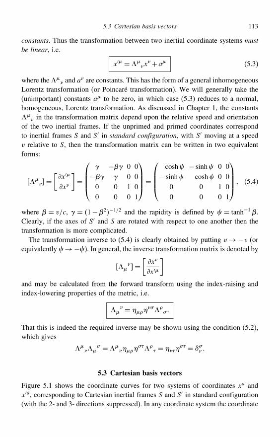
5.3 Cartesian basis vectors 113
constants. Thus the transformation between two inertial coordinate systems mustbe linear, i.e.
x′ =$x
+a (5.3)
where the$ and a
are constants. This has the form of a general inhomogeneousLorentz transformation (or Poincaré transformation). We will generally take the(unimportant) constants a to be zero, in which case (5.3) reduces to a normal,homogeneous, Lorentz transformation. As discussed in Chapter 1, the constants$
in the transformation matrix depend upon the relative speed and orientationof the two inertial frames. If the unprimed and primed coordinates correspondto inertial frames S and S′ in standard configuration, with S′ moving at a speedv relative to S, then the transformation matrix can be written in two equivalentforms:
$=
[x′
x
]=
⎛⎜⎜⎜⎝ − 0 0− 0 00 0 1 00 0 0 1
⎞⎟⎟⎟⎠=⎛⎜⎜⎜⎝
cosh − sinh 0 0− sinh cosh 0 0
0 0 1 00 0 0 1
⎞⎟⎟⎟⎠ (5.4)
where = v/c, = 1−2−1/2 and the rapidity is defined by = tanh−1.Clearly, if the axes of S′ and S are rotated with respect to one another then thetransformation is more complicated.
The transformation inverse to (5.4) is clearly obtained by putting v→−v (orequivalently →−). In general, the inverse transformation matrix is denoted by
$=
[x
x′
]and may be calculated from the forward transform using the index-raising andindex-lowering properties of the metric, i.e.
$ =
#$#
That this is indeed the required inverse may be shown using the condition (5.2),which gives
$$
# =$
#$ =
# = #
5.3 Cartesian basis vectors
Figure 5.1 shows the coordinate curves for two systems of coordinates xa andx′a, corresponding to Cartesian inertial frames S and S′ in standard configuration(with the 2- and 3- directions suppressed). In any coordinate system the coordinate
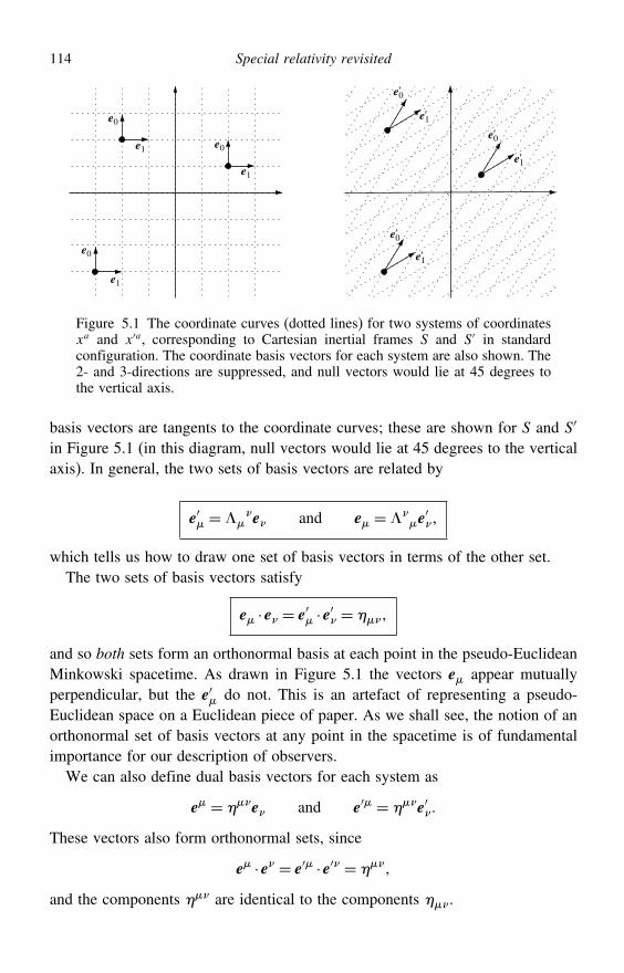
114 Special relativity revisited
e1
e0
e1
e1
e0
e0
e0'
e1'
e1'
e1'
e0'
e0'
Figure 5.1 The coordinate curves (dotted lines) for two systems of coordinatesxa and x′a, corresponding to Cartesian inertial frames S and S′ in standardconfiguration. The coordinate basis vectors for each system are also shown. The2- and 3-directions are suppressed, and null vectors would lie at 45 degrees tothe vertical axis.
basis vectors are tangents to the coordinate curves; these are shown for S and S′in Figure 5.1 (in this diagram, null vectors would lie at 45 degrees to the verticalaxis). In general, the two sets of basis vectors are related by
e′ =$e and e =$
e′
which tells us how to draw one set of basis vectors in terms of the other set.The two sets of basis vectors satisfy
e · e = e′ · e′ =
and so both sets form an orthonormal basis at each point in the pseudo-EuclideanMinkowski spacetime. As drawn in Figure 5.1 the vectors e appear mutuallyperpendicular, but the e′ do not. This is an artefact of representing a pseudo-Euclidean space on a Euclidean piece of paper. As we shall see, the notion of anorthonormal set of basis vectors at any point in the spacetime is of fundamentalimportance for our description of observers.
We can also define dual basis vectors for each system as
e = e and e′ = e′
These vectors also form orthonormal sets, since
e · e = e′ · e′ =
and the components are identical to the components .
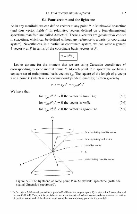
5.4 Four-vectors and the lightcone 115
5.4 Four-vectors and the lightcone
As in any manifold, we can define vectors at any point P in Minkowski spacetime(and thus vector fields).4 In relativity, vectors defined on a four-dimensionalspacetime manifold are called 4-vectors. These 4-vectors are geometrical entitiesin spacetime, which can be defined without any reference to a basis (or coordinatesystem). Nevertheless, in a particular coordinate system, we can write a general4-vector v at P in terms of the coordinate basis vectors at P:
v= ve
Let us assume for the moment that we are using Cartesian coordinates x
corresponding to some inertial frame S. At each point P in spacetime we have aconstant set of orthonormal basis vectors e. The square of the length of a vectorv at a point P (which is a coordinate-independent quantity) is then given by
v · v= vv = v
v
We have thatfor v
v > 0 the vector is timelike (5.5)
for vv = 0 the vector is null (5.6)
for vv < 0 the vector is spacelike (5.7)
e0
e2
e1
future-pointing timelike vector
future-pointing null vector
spacelike vector
past-pointing timelike vector
Figure 5.2 The lightcone at some point P in Minkowski spacetime (with onespatial dimension suppressed).
4 In fact, since Minkowski spacetime is pseudo-Euclidean, the tangent space TP at any point P coincides withthe manifold itelf. Thus, in this special case, we are not restricted to local vectors and can reinstate the notionsof position vector and of the displacement vector between arbitrary points in the manifold.
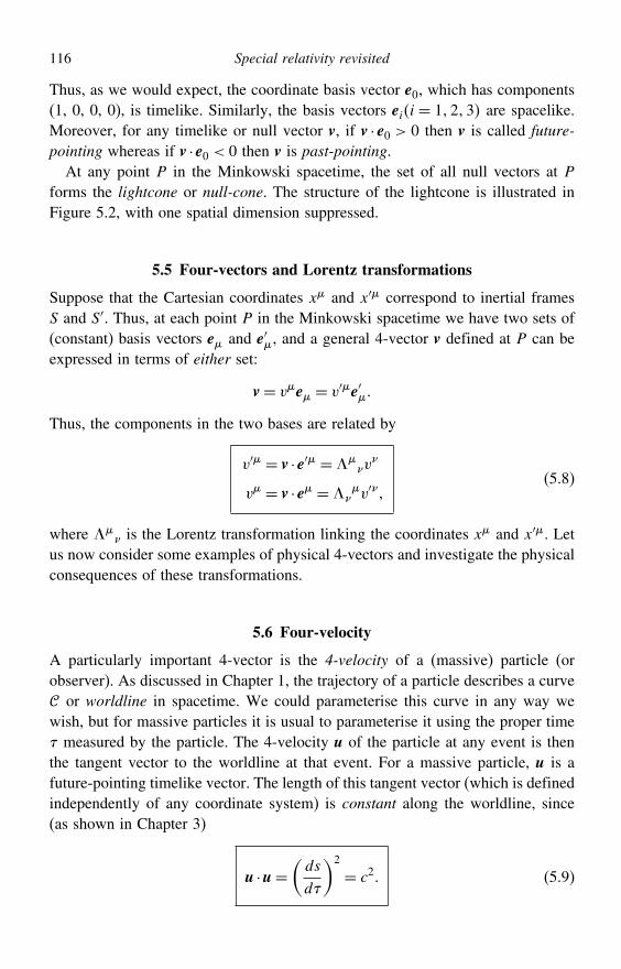
116 Special relativity revisited
Thus, as we would expect, the coordinate basis vector e0, which has components(1, 0, 0, 0), is timelike. Similarly, the basis vectors eii = 123 are spacelike.Moreover, for any timelike or null vector v, if v · e0 > 0 then v is called future-pointing whereas if v · e0 < 0 then v is past-pointing.
At any point P in the Minkowski spacetime, the set of all null vectors at Pforms the lightcone or null-cone. The structure of the lightcone is illustrated inFigure 5.2, with one spatial dimension suppressed.
5.5 Four-vectors and Lorentz transformations
Suppose that the Cartesian coordinates x and x′ correspond to inertial framesS and S′. Thus, at each point P in the Minkowski spacetime we have two sets of(constant) basis vectors e and e′, and a general 4-vector v defined at P can beexpressed in terms of either set:
v= ve = v′e′
Thus, the components in the two bases are related by
v′ = v · e′ =$v
v = v · e =$v′
(5.8)
where $ is the Lorentz transformation linking the coordinates x and x′. Let
us now consider some examples of physical 4-vectors and investigate the physicalconsequences of these transformations.
5.6 Four-velocity
A particularly important 4-vector is the 4-velocity of a (massive) particle (orobserver). As discussed in Chapter 1, the trajectory of a particle describes a curve or worldline in spacetime. We could parameterise this curve in any way wewish, but for massive particles it is usual to parameterise it using the proper time measured by the particle. The 4-velocity u of the particle at any event is thenthe tangent vector to the worldline at that event. For a massive particle, u is afuture-pointing timelike vector. The length of this tangent vector (which is definedindependently of any coordinate system) is constant along the worldline, since(as shown in Chapter 3)
u ·u=(ds
d
)2
= c2 (5.9)
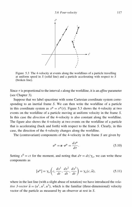
5.6 Four-velocity 117
x0
x1
Figure 5.3 The 4-velocity at events along the worldlines of a particle travellingat uniform speed in S (solid line) and a particle accelerating with respect to S(broken line).
Since is proportional to the interval s along the worldline, it is an affine parameter(see Chapter 3).
Suppose that we label spacetime with some Cartesian coordinate system corre-sponding to an inertial frame S. We can then write the worldline of a particlein this coordinate system as x = x. Figure 5.3 shows the 4-velocity at twoevents on the worldline of a particle moving at uniform velocity in the frame S.In this case the direction of the 4-velocity is also constant along the worldline.The figure also shows the 4-velocity at two events on the worldline of a particlethat is accelerating (back and forth) with respect to the frame S. Clearly, in thiscase, the direction of the 4-velocity changes along the worldline.
The (contravariant) components of the 4-velocity in the frame S are given by
u = u · e = dx
d (5.10)
Setting x0 = ct for the moment, and noting that d = dt/u, we can write thesecomponents as
u= u
(c
dx1
dtdx2
dtdx3
dt
)= uc u (5.11)
where in the last line (with a slight abuse of notation) we have introduced the rela-tive 3-vector u = u1 u2 u3, which is the familiar (three-dimensional) velocityvector of the particle as measured by an observer at rest in S.
118 Special relativity revisited
In some other inertial frame S′, the components of the 4-velocity of the parti-cle are
u′ = u · e′ =$u
Writing this out in full for the case where S and S′ are in standard configurationwith relative speed v, we obtain⎛⎜⎜⎜⎝
u′c
u′u′1
u′u′2
u′u′3
⎞⎟⎟⎟⎠=⎛⎜⎜⎜⎝
v −v 0 0−v v 0 00 0 1 00 0 0 1
⎞⎟⎟⎟⎠⎛⎜⎜⎜⎝uc
uu1
uu2
uu3
⎞⎟⎟⎟⎠
This is equivalent to four equations. From the first, we find that
uu′
= 1v
11−u1v/c2
and from the others we obtain the 3-velocity addition law in special relativity,
u′1 = u1−v
1−u1v/c2
u′2 = u2
v1−u1v/c2
u′3 = u3
v1−u1v/c2
Note that this approach has allowed us to derive the 3-velocity addition law in analmost trivial way.
5.7 Four-momentum of a massive particle
The 4-momentum of a massive particle of rest mass m0 is defined in terms of itsfour-velocity u by
p=m0u
At any point P along the particle’s worldline the square of the length of thisvector is
p ·p=m0u ·m0u=m20c
2 (5.12)
In Cartesian coordinates x corresponding to some inertial frame S, the compo-nents of the 4-momentum are simply p= p ·e. According to convention we write
p= E/cp1 p2 p3= E/c p (5.13)
5.8 Four-momentum of a photon 119
where E is the energy of the particle as measured in the frame S and p is its3-momentum measured in S. Comparing (5.13) with (5.11) we see that, in specialrelativity,
E = um0c2 (5.14)
p = um0u (5.15)
In the frame S, the squared length of the 4-momentum is given by pp. Thus,from (5.13) and (5.12), we find that
E2−p2c2 =m20c
4
where p2 = p · p. This is the well-known energy–momentum invariant.
5.8 Four-momentum of a photon
The above discussion concerned particles of non-zero rest mass, which moveat speeds less than c. We now consider particles such as photons and perhapsneutrinos, which move at the speed of light. The worldline of a massless particle isa null curve, along which d = 0. Thus, we cannot parameterise such a worldlineusing the proper time . Nevertheless, there are many other parameters that wecan use. For example, in an inertial frame, a photon travelling in the positivex-direction will describe the path x = ct. This could be written parametrically as
x = u# (5.16)
where # is the parameter and u= 1100. Using (3.43), the tangent vectorto the worldline is then
u= dx
d#e = ue
Since the worldline is a null curve, we have
u ·u= 0 (5.17)
in contrast with (5.9). Moreover, with this choice of parameter we see that
dud#
= 0 (5.18)
which is the equation of motion for a photon. We note that although this hasbeen derived using the fact that the Cartesian basis vectors e do not changewith position, it is a vector equation and therefore will hold in any basis (i.e. anycoordinate system).
120 Special relativity revisited
Our choice of parameterisation in (5.16) may appear somewhat arbitrary.Indeed, it is true that there exists an unlimited number of parameterisations thatcould be used. For example, suppose that we replaced # by 2 (say). As the newparameter varies between − and , the same worldline x = ct would bedescribed in the spacetime. Since this is a null curve, the condition (5.17) wouldcontinue to be true (as may be verified explicitly). In the new parameterisation,however, the equation of motion (5.18) would not still hold. The special class ofparameters for which the equation of motion has the simple form (5.18) is theclass of affine parameters (as discussed in Section 3.16). Since one is always freeto choose such a parameter, we will assume from here on that equation (5.18) issatisfied.
So far, we have not mentioned the frequency (or energy) of the photon, whichcharacterises it in much the same way as the rest mass m0 characterises a massiveparticle. Clearly, the tangent vector u can be multipled by any scalar constant andwill still satisfy the equations (5.17) and (5.18). The 4-momentum of a photon istherefore defined as
p= u
for a constant chosen such that, in an arbitrary inertial frame S, the componentsof p are
p= E/c pwhere E is the energy of the photon as measured in S and p is its 3-momentumin S. From (5.17) we thus have E = pc.
For photons, it is also common to introduce the 4-wavevector k, which is relatedto the four-momentum by p = k. Thus, in the frame S, the 4-wavevector hascomponents given by
k= 2/ kwhere is the wavelength of the photon as measured in S and k= 2/n andn is a unit 3-vector in the direction of propagation.
5.9 The Doppler effect and relativistic aberration
An example of the usefulness of the 4-vector approach (and particularly the photon4-wavevector) is provided by the Doppler effect. Suppose that an observer is atrest in some Cartesian inertial frame S defined by the coordinates x in spacetime.Let us also suppose that a source of radiation is moving relative to S with a speedv in the positive x1-direction and that at some event P the observer receives aphoton of wavelength in a direction that makes an angle with the positive
5.9 The Doppler effect and relativistic aberration 121
x1-direction. Thus, at the event P the components k = k · e of the photon’s4-wavevector in this coordinate system are
k= 21 cos sin 0
The photon observed at the event P must have been emitted by the source at someother event Q (say). However, the equation of motion of a photon implies thatits 4-momentum p, and hence its 4-wavevector k, is constant along its worldline.Thus the photon’s 4-wavevector k at the event Q is the same as that at theevent P.
Let us denote the Cartesian inertial frame in which the radiation source is atrest by S′ (whose spatial axes are assumed not to be rotated with respect to thoseof S); this frame is represented by the coordinates x′ in spacetime. Thus, atthe event Q the components in S′ of the photon’s 4-wavevector are given byk′ = k · e′ and read
k′ =$k
(5.19)
where $ is given by (5.4).
We denote these components in S′ by
k′= 2′
1 cos′ sin ′0
The zeroth component of (5.19) yields the ratio of the proper wavelength and theobserved wavelength:
′
= 1− cos
This equation contains all the familiar Doppler effect results as special cases. If = 0, the source must be approaching the observer along the negative x1-axis.If = , the source is receding from the observer along the positive x1-axis.Finally, if =±/2 we obtain the transverse Doppler effect. Similarly, from the2- and 3- components of (5.19) we obtain immediately
tan ′ = tan 1− v/c sec
which is a version of the relativistic aberration formula.
122 Special relativity revisited
5.10 Relativistic mechanics
In relativistic mechanics, the equation of motion of a massive particle is given by
dpd= f
where f is the 4-force. In some Cartesian inertial frame S (for which the basisvectors are constant throughout the spacetime) the components f of the 4-forceare given by the familiar expression
f = e · dpd= e · d
dpe=
dp
d =
dp
d
where we have used the fact that e and e are reciprocal sets of vectors. Notingthat d = dt/u, we may write
f= ud
dt
(E
c p)= u
( f · uc
f)
where in the last equality we have introduced the familiar 3-force f as measuredin the frame S, and u is the 3-velocity in this frame. Writing the compo-nents in this way, the time and space parts of the equation of motion in S are(as required)
1u
dE
d= dE
dt= f · u (5.20)
1u
dpd
= dpdt= f (5.21)
where E and p are given by (5.14) and (5.15) respectively.There is, however, a certain rarely discussed subtlety in relativistic mechan-
ics. Let us consider the scalar product u · f , which is of course invariant undercoordinate transformations. This is given by
u · f = u · dpd
= u ·(dm0
du+m0
dud
)= c2
dm0
d+m0u ·
dud
= c2dm0
d
where we have (twice) used the fact that u ·u= c2. Thus, we see that in specialrelativity the action of a force can alter the rest mass of a particle! A force thatpreserves the rest mass is called a pure force and must satisfy u · f = 0.
5.12 Relativistic collisions and Compton scattering 123
If so desired, one can also introduce the 4-acceleration of a particle, a= du/d,in terms of which a pure 4-force takes the familiar form f = m0a. In someCartesian inertial frame S, the components of the 4-acceleration are
a=[du
d
]= u
d
dtucuu = u
(cdudt
ududt+ udu
dt
)
= u
(cdudt
ua+ ududt
)
where a= du/dt is the 3-acceleration in the frame S.
5.11 Free particles
We now come to a very important observation concerning relativistic mechanics.In the absence of any forces, the equation of motion of a massive particle is
dpd= 0 (5.22)
where the proper time is an affine parameter along the particle’s worldline.Similarly, the equation of motion of a photon is
dpd#
= 0 (5.23)
where # is some affine parameter along the photon’s worldline. However, in eachcase the 4-momentum p at some point on the worldline is simply a fixed multipleof the tangent vector to the worldline at that point. Thus, equations (5.22) and(5.23) say that tangent vectors to the worldlines of free particles and of photonsform a parallel field of vectors along the worldline. From Chapter 2 we knowthat this is the definition of an affinely parameterised geodesic. Thus, in specialrelativity the worldlines of free particles and photons are respectively non-nulland null geodesics in Minkowski spacetime.
5.12 Relativistic collisions and Compton scattering
We note from (5.22) and (5.23) that the conservation of energy and momentumfor a free particle or photon is represented by the single equation p = constant.We can, of course, add the 4-momenta of different particles. Thus for a system ofn interacting particles i= 12 n with no external forces, we have
∑ni=1 pi =
constant, which is very useful in relativistic-collision calculations.
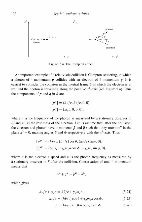
124 Special relativity revisited
θ
electron
photon
φ
x2 x2
x1 x1
photon
electron
Figure 5.4 The Compton effect.
An important example of a relativistic collision is Compton scattering, in whicha photon of 4-momentum p collides with an electron of 4-momentum q. It iseasiest to consider the collision in the inertial frame S in which the electron is atrest and the photon is travelling along the positive x1-axis (see Figure 5.4). Thusthe components of p and q in S are
p = h/ch/c00
q = mec000
where is the frequency of the photon as measured by a stationary observer inS, and me is the rest mass of the electron. Let us assume that, after the collision,the electron and photon have 4-momenta p and q such that they move off in theplane x3 = 0, making angles and respectively with the x1-axis. Thus
p = h/c h/c cos h/c sin 0
q = umecumeu cos−ume sin0
where u is the electron’s speed and is the photon frequency as measured bya stationary observer in S after the collision. Conservation of total 4-momentummeans that
p+q = p+ q
which gives
h/c+mec = h/c+umec (5.24)
h/c = h/c cos+umeu cos (5.25)
0 = h/c sin −umeu sin (5.26)
5.13 Accelerating observers 125
Eliminating u and from these equations leads to the formula for Comptonscattering, which gives the frequency of the photon in S after the collision:
=
[1+ h
mec21− cos
]−1
The components of the 4-momentum p (or q) in any other inertial frame S′can be found easily by using p′ = $
p, where $
are the elements of theLorentz transformation matrix connecting the frames S and S′.
5.13 Accelerating observers
So far we have only considered inertial observers, who move at uniform speedswith respect to one another. Let us now consider a general observer , whomay be accelerating with respect to some inertial frame S. If the observer has a4-velocity u, where is the proper time measured along the worldline, thenhis 4-acceleration is given by
a= dud
It is worth noting that, at any given event P, the 4-acceleration a is alwaysorthogonal to the corresponding 4-velocity u, since
a ·u= d
d
( 12u ·u
)= d
d
( 12c
2)= 0 (5.27)
An accelerating observer has no inertial frame in which he or she is always atrest. Nevertheless, at any event P along the worldline we can define an instan-taneous rest frame S′, in which the observer is momentarily at rest. Sincethe observer is at rest in S′, the timelike basis vector e′0 of this frame must beparallel to the 4-velocity u of the observer. The remaining spacelike basis vectorse′i (i= 123) of S′ are all orthogonal to e′0 and to one another and will depend onthe relative velocity of S and S′ and the relative orientation of their spatial axes.Observations made by at the event P thus correspond to measurements madein the instantaneous rest frame (IRF) S′ at P. This is illustrated in Figure 5.5.
Thus, the notion of a localised laboratory can be idealised as follows. Anobserver (whether accelerating or not) carries along four orthogonal unit vectorse′ (or tetrad), which vary along his worldline but always satisfy
e′ · e′= (5.28)
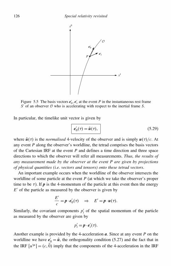
126 Special relativity revisited
P
x0
x1
e0'
e1'
Figure 5.5 The basis vectors e′0 e′1 at the event P in the instantaneous rest frame
S′ of an observer who is accelerating with respect to the inertial frame S.
In particular, the timelike unit vector is given by
e′0= u (5.29)
where u is the normalised 4-velocity of the observer and is simply u/c. Atany event P along the observer’s worldline, the tetrad comprises the basis vectorsof the Cartesian IRF at the event P and defines a time direction and three spacedirections to which the observer will refer all measurements. Thus, the results ofany measurement made by the observer at the event P are given by projectionsof physical quantities (i.e. vectors and tensors) onto these tetrad vectors.
An important example occurs when the worldline of the observer intersects theworldline of some particle at the event P (at which we take the observer’s propertime to be ). If p is the 4-momentum of the particle at this event then the energyE′ of the particle as measured by the observer is given by
E′
c= p · e′0 ⇒ E′ = p ·u
Similarly, the covariant components p′i of the spatial momentum of the particleas measured by the observer are given by
p′i = p · e′iAnother example is provided by the 4-acceleration a. Since at any event P on theworldline we have e′0 = u, the orthogonality condition (5.27) and the fact that in
the IRF u′= c 0 imply that the components of the 4-acceleration in the IRF
5.13 Accelerating observers 127
are a′ = 0 a′. Thus the magnitude of the 3-acceleration in the IRF can becomputed as the simple invariant a ·a.
It is interesting to consider how the tetrad of basis vectors changes alongthe worldline of an observer whose acceleration varies arbitrarily with time.As it is transported along the observer’s worldline, the tetrad must satisfy thetwo requirements (5.28) and (5.29). Clearly, given u the condition (5.29)determines the timelike basis vector e′0 uniquely. Unfortunately, condition(5.28) is obviously insufficient to determine uniquely the evolution of the spacelikebasis vectors e′ii = 123, which reflect the different ways in which theobserver’s local laboratory might be spinning and tumbling. An important specialcase, however, is when the tetrad is ‘non-rotating’.
This last requirement requires some clarification. Clearly, the basis vectors ofthe tetrad at any proper time are related to the basis vectors e of some giveninertial frame by the Lorentz transformation
e′=$e
Thus the tetrad basis vectors at two successive instants must also be related to eachother by a Lorentz transformation, which can be thought of as a ‘rotation’ in space-time.A ‘non-rotating’ tetrad is onewhere the basis vectors e′ change from instantto instant by precisely the amount implied by the rate of change of u but with noadditional rotation. In other words, we accept the inevitable rotation in the timelikeplane defined by u and a but rule out any ordinary rotation of the 3-space vectors.
Since we wish to treat the time and space directions on an equal footing, we mustseek a general expression for the rate of change de′/d of a basis vector alongthe worldline such that: (i) it generates the appropriate Lorentz transformation ife′ lies in the timelike plane defined by u and a, and (ii) it excludes any rotationif e′ lies in any other plane, in particular any spacelike plane. A little reflectionshows that the unique answer to these requirements is
de′d
= 1c2[u · e′a− a · e′u
] (5.30)
Any vector that undergoes the above transformation is said to be Fermi–Walkertransported along the worldline. From (5.30), we find that if e′ is orthogonal toboth u and a then de′/d = 0 as required. Moreover, we see that de′0/d = a/c,again as required.
A physical example of a 3-space vector that does not rotate along the worldlineis the spin (i.e. the angular momentum vector) of a gyroscope that the observeraccelerates with himself by means of forces applied to its centre of mass (so that
128 Special relativity revisited
there are no torques). Indeed, a careful observer could set up a non-rotating tetradby aligning his three spatial axes using such gyroscopes.
5.14 Minkowski spacetime in arbitrary coordinates
There is no need to label events in Minkowski spacetime with the Cartesianinertial coordinates we have used thus far. The advantage of Cartesian coordinatesX, which put the line element into the form5
ds2 = dXdX (5.31)
(even just at a particular event P), is that they have a clear physical meaning, i.e.they correspond to time and distances measured by an observer at P who is at restin some inertial frame S labelled using three-dimensional Cartesian coordinates(we will prove this below). Nevertheless, we are free to label events in spacetimeusing any arbitrary system of coordinates x although, in general, the coordinatesin such an arbitrary system may not have simple physical meanings.
Since the path of a free massive particle is a geodesic in Minkowski spacetime,its worldline x in some arbitrary coordinate system is given by the geodesicequations
d2x
d2+
#
dx
d
dx#
d= 0 (5.32)
An inertial frame S is defined as one in which a free particle moves in a straightline with fixed speed. Thus from (5.31) it is clear that coordinates X, such that(5.31) holds, define an inertial frame. In this case, the connection
# vanishes,and so the worldline of a particle is given by
d2X
d2= 0 (5.33)
Setting X = cTXYZ for the moment, the = 0 equation (5.33) showsthat dT/d = constant. Thus the = 123 equations read
d2X
dT 2= d2Y
dT 2= d2Z
dT 2= 0
from which we see immediately that a free particle moves in a straight line withconstant speed in S.
We could label the inertial frame S using three-dimensional spatial coordi-nates that are not Cartesian, however. For example, we could use spherical polar
5 In the interest of clarity, in this section we will denote Cartesian inertial coordinates by X and an arbitrarycoordinate system by x.
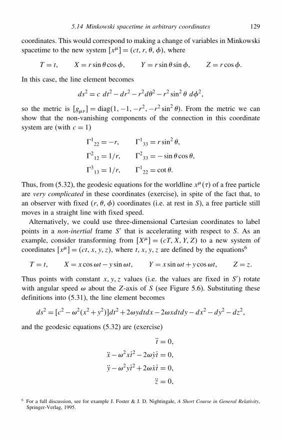
5.14 Minkowski spacetime in arbitrary coordinates 129
coordinates. This would correspond to making a change of variables in Minkowskispacetime to the new system x= ct r , where
T = t X = r sin cos Y = r sin sin Z = r cos
In this case, the line element becomes
ds2 = c dt2−dr2− r2d2− r2 sin2 d2
so the metric is g = diag1−1−r2−r2 sin2 . From the metric we canshow that the non-vanishing components of the connection in this coordinatesystem are (with c = 1)
122 =−r 1
33 = r sin2
212 = 1/r 2
33 =− sin cos
313 = 1/r 1
22 = cot
Thus, from (5.32), the geodesic equations for the worldline x of a free particleare very complicated in these coordinates (exercise), in spite of the fact that, toan observer with fixed r coordinates (i.e. at rest in S), a free particle stillmoves in a straight line with fixed speed.
Alternatively, we could use three-dimensional Cartesian coordinates to labelpoints in a non-inertial frame S′ that is accelerating with respect to S. As anexample, consider transforming from X = cTXYZ to a new system ofcoordinates x= ct x y z, where t x y z are defined by the equations6
T = t X = x cost−y sint Y = x sint+y cost Z = z
Thus points with constant x y z values (i.e. the values are fixed in S′) rotatewith angular speed about the Z-axis of S (see Figure 5.6). Substituting thesedefinitions into (5.31), the line element becomes
ds2 = c2−2x2+y2dt2+2ydtdx−2xdtdy−dx2−dy2−dz2
and the geodesic equations (5.32) are (exercise)
t = 0
x−2xt2−2yt = 0
y−2yt2+2xt = 0
z = 0
6 For a full discussion, see for example J. Foster & J. D. Nightingale, A Short Course in General Relativity,Springer-Verlag, 1995.
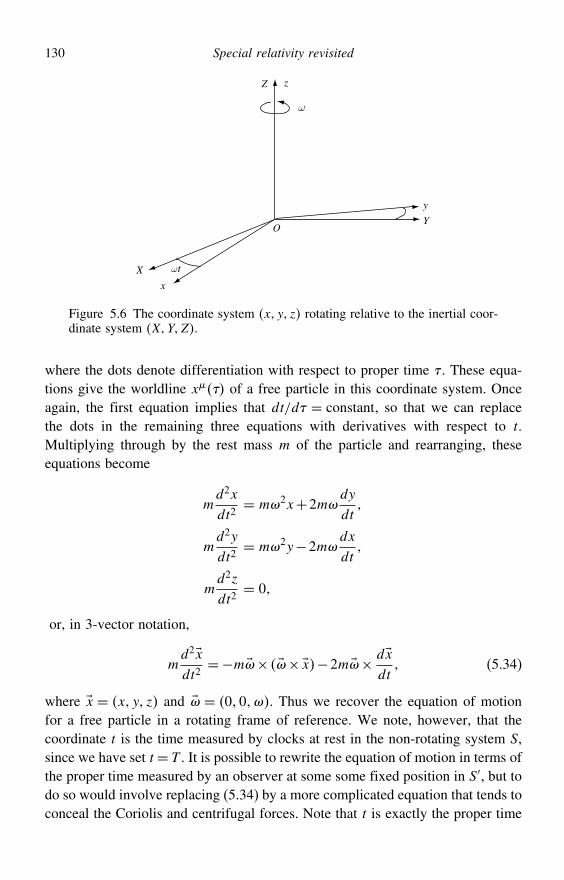
130 Special relativity revisited
ω
Y
y
X
x
ω t
O
Z z
Figure 5.6 The coordinate system x y z rotating relative to the inertial coor-dinate system XYZ.
where the dots denote differentiation with respect to proper time . These equa-tions give the worldline x of a free particle in this coordinate system. Onceagain, the first equation implies that dt/d = constant, so that we can replacethe dots in the remaining three equations with derivatives with respect to t.Multiplying through by the rest mass m of the particle and rearranging, theseequations become
md2x
dt2= m2x+2m
dy
dt
md2y
dt2= m2y−2m
dx
dt
md2z
dt2= 0
or, in 3-vector notation,
md2xdt2
=−m× ×x−2m× dxdt
(5.34)
where x = x y z and = 00. Thus we recover the equation of motionfor a free particle in a rotating frame of reference. We note, however, that thecoordinate t is the time measured by clocks at rest in the non-rotating system S,since we have set t= T . It is possible to rewrite the equation of motion in terms ofthe proper time measured by an observer at some some fixed position in S′, but todo so would involve replacing (5.34) by a more complicated equation that tends toconceal the Coriolis and centrifugal forces. Note that t is exactly the proper time
Exercises 131
for an observer situated at the common origin O of the two systems, so observersclose to O who are at rest in S′ would accept (5.34) as (approximately) valid.From these examples, we see that in general the geodesic equations can be
rather complicated both for non-inertial frames and for inertial frames labelledby non-Cartesian spatial coordinates. Thus, when describing physical effects inan inertial frame, it is conventional to use Cartesian spatial coordinates to labelpoints in the frame and so to work in a coordinate system X for which (5.31) isvalid. It is then much easier to disentangle the physical effects from artefacts ofthe coordinate system.
Exercises
5.1 Show that the transformation matrix for a Lorentz transformation from S to S′ instandard configuration is given by (5.4).
5.2 Show that, under a Lorentz transformation, the covariant components of a vectortransform as v′ = $
v. Hence show explicitly in component form that, for two4-vectors v and w, the scalar product v ·w is invariant under a Lorentz transformation.
5.3 Prove that, for any timelike vector v in Minkowski space, there exists an inertialframe in which the spatial components are zero.
5.4 Prove (a) that the sum of any two spacelike vectors is spacelike; and (b) that atimelike vector and a null vector cannot be orthogonal.
5.5 For the spaceship discussed in Section 1.14, which maintains a uniform accelerationa in the x-direction of some inertial frame S, the worldline is given by
t= c
asinh
a
c x= c2
a
(cosh
a
c−1
) y= 0 z= 0
where is the proper time of an astronaut on the spaceship. Show that the 4-velocityof the rocket in the coordinate system ct x y z is given by
u=(c cosh
a
c c sinh
a
c00
)
Hence show explicitly that uu = c2 and that the spaceship’s 3-velocity is
u=(c tanh
a
c00
)
5.6 Show that the 4-acceleration of the spaceship in Exercise 5.5 is given by
a=(a sinh
a
ca cosh
a
c00
)
Hence show that aa = a2 and that the magnitude of the spaceship’s 3-accelerationin its own instantaneous rest frame is also a.
5.7 A spaceship has constant acceleration g in the x-direction in its locally comovingframe, i.e. the IRF. Show that, in an inertial frame, the spaceship’s 4-velocity u=
132 Special relativity revisited
u0 u100 and 4-acceleration a = a0 a100 satisfy a1 = gu0/c and a0 =gu1/c. Show also that
d2u
d2= g2u
c2
where is the proper time as measured by an occupant of the spaceship. A spaceshipaccelerates at a constant rate g = 95m s−2 in its own locally comoving frame.It starts out towards the centre of the Galaxy 10 kpc distant. After going 5 kpcit decelerates at the same rate to come to rest again at the Galactic centre. Theoutward journey is then repeated in reverse to come back home. Show that, in thespaceship’s frame, the elapsed travel time is 41.5 years. What is the elapsed timefor the waiting observer (or descendants) on Earth?
5.8 Show that in its own instantaneous rest frame (IRF), a particle’s 4-acceleration isgiven by a= 0 a, where a is the 3-acceleration of the particle in the IRF.
5.9 Show that, in an inertial frame in which a particle’s 3-acceleration a is orthogonalto its 3-velocity u, the particle’s 4-acceleration is given by a= 2
u0 a.5.10 Show that when an electron and a positron annihilate, more than one photon must
be produced.5.11 Show that if a photon is reflected from a mirror moving parallel to its plane, then
the angle of incidence of the photon is equal to the angle of reflection.5.12 An inertial frame S′ moves with constant velocity u along the x-axis with respect
to frame S. A photon in frame S′ is fired at an angle ′ to the forward direction ofmotion. Show that the angle measured in frame S is
tan = tan ′1−21/2
1+ sec′
where = u/c.5.13 A photon with energy E collides with a stationary electron whose rest mass is m0.
As a result of the collision the direction of the photon’s motion is deflected throughan angle and its energy is reduced to E′. Show that
m0c2
(1E′− 1
E
)= 1− cos
Deduce that the wavelength of the photon is increased by
= 2hm0c
sin2(
2
)
where h is Planck’s constant. At what angle to the initial photon direction doesthe electron move? Show that, if the photon is deflected through a right angle, andthe photon energy satisfies E m0c
2, then after the interaction the angle of theelectron’s motion to the direction of the photon’s initial motion is =−/4.
5.14 Inverse Compton scattering occurs whenever a photon scatters off a particle movingwith a speed very nearly equal to that of light. Suppose that a particle of rest mass
Exercises 133
m0 and total energy E collides head on with a photon of energy E . Show that thescattered photon has energy
E
(1+ m2
0c4
4EE
)−1
Ultra-high-energy cosmic rays have energies up to 1020 eV. How much energy cana cosmic ray proton transfer to a microwave background photon?
5.15 For a pure 4-force f acting on a particle of rest massm0, show that the corresponding3-force f satisfies
f = um0a+f · uc2u
Hence show that a is only parallel to f when f is either parallel or orthogonalto u. Show further that, in these two cases, one has f = 3
um0a and f = um0arespectively.
5.16 For a pure 4-force f acting on a particle of rest mass m0, show that
m0
dud= u
f 5.17 In Minkowski spacetime, consider an emitter moving at speed v along the positive
x1-axis of the frame S in which a receiver is at rest. Prove the Doppler shiftformula
= v
(1− v
ccos
)
where is the angle made by the photon trajectory with the x1-axis of S. Show thatthis expression can be written in the manifestly covariant way
= uk
uk
where k is the photon 4-wavevector and u and u are the 4-velocities of and respectively.
5.18 An astronaut on the space rocket in Exercise 5.5 refers all his measurements to anorthonormal tetrad !e′" that comprises the basis vectors of a Cartesian instan-taneous rest frame S′ at proper time . Suppose that at = 0 the tetrad coincideswith the fixed basis vectors !e" of the ct x y z coordinate system in the inertialframe S and that the rocket is not rotating in any way. Show that, in the ct x y zcoordinate system, the components of the astronaut’s orthonormal tetrad at somelater proper time are
e′0 =(cosh
a
c sinh
a
c00
)
e′1 =(sinh
a
c cosh
a
c00
)
e′2 = 0010
e′3 = 0001
134 Special relativity revisited
The astronaut observes photons that were emitted with frequency 0 from a star thatis stationary at the origin of S. Show that the frequency of the photons as measuredby the astronaut at proper time is given by
= 0 exp−a/c5.19 At some event P in Minkowski spacetime, the worldline of a particle (either massive
or massless) and an observer cross. If, at this event, the particle has 4-momentump and the observer has 4-velocity u then show that the observer measures themagnitude of the spatial momentum of the particle to be
p =[p ·u2c2
−p ·p]1/2
5.20 Repeat Exercise 1.10 using 4-vectors.5.21 In Minkowski spacetime, the coordinates cTXYZ correspond to a Cartesian
inertial frame. The coordinates ct r are related to them by the equations
X = r sin cos Y = r sin sin Z = r cos
Obtain the special-relativistic equations of motion of a free particle in the ct r coordinate system, and interpret these equations physically.
5.22 Repeat Exercise 5.21 for the coordinates ct z, that are related to the Cartesianinertial coordinates cTXYZ by
T = t
X = cos cost− sin sint
Y = cos sint+ sin cost
Z = z
where is a constant.
6
Electromagnetism
At the time special relativity was devised only two forces were known, electro-magnetism and gravity. As mentioned in Chapter 1, it was electromagnetism thatactually led to the development of special relativity. Therefore, we now discusselectromagnetism in some detail; in particular its relativistic formulation. Thiswill introduce a number of ideas that we will use later in developing and applyinga relativistic formulation of gravity, namely general relativity. Our guiding prin-ciple here is to derive tensorial equations in Minkowski spacetime. This makesit possible to express the theory in a form that is independent of the coordinatesystem used. We will see that a consistent theory of electromagnetism followsfrom saying that there exists a pure 4-force that depends linearly on 4-velocityand also on a certain property of a particle, namely its charge q. Even if one hasno prior knowledge of electromagnetism, one can derive the complete theory ina few lines using this basic assumption and occasional appeals to simplicity.
6.1 The electromagnetic force on a moving charge
In some inertial frame S, the 3-force on a particle of charge q moving in anelectromagnetic field is
f = qE+ u× Bwhere u is the particle’s 3-velocity in S. The 3-vector fields E and B are theelectric and magnetic fields as measured in S. This equation suggests that for theproper relativistic formulation we should write down a tensor equation in four-dimensional spacetime in which the electromagnetic 4-force f depends linearlyon the particle’s 4-velocity u. Thus we are led to an equation of the form
f = qF ·u (6.1)
135
136 Electromagnetism
where F must be a rank-2 tensor in order to make a 4-force from a 4-velocity.We call F the electromagnetic field tensor. The scalar q is some property of theparticle that determines the strength of the electromagnetic force upon it (i.e. itscharge).
We could develop the theory entirely in terms of coordinate-independent4-vectors and 4-tensors. Nevertheless, if we label points in spacetime with somearbitrary coordinate system x, we may express (6.1) in component form as
f = qFu
where the F are the covariant components of F in our chosen coordinatesystem. In order that the rest mass of a particle is not altered by the action ofthe electromagnetic force we require the latter to be a pure force, so that for any4-velocity u we have u · f = 0. In component form this reads
fu = qFu
u = 0
which implies that the electromagnetic field tensor must be antisymmetric, i.e.
F =−F
The contravariant components of F are given by
F = g#gF#
where the g are the contravariant components of the metric tensor in ourcoordinate system. Since g is symmetric, it is clear that F =−F also.
6.2 The 4-current density
So far we have found only the relativistic form of the electromagnetic force onan idealised point particle with charge q and 4-velocity u, in terms of some asyet undetermined rank-2 antisymmetric tensor F. In order to develop the theoryfurther, we must now construct the field equations of the theory, which determinethe electromagnetic field tensor Fx at any point in spacetime in terms of chargesand currents. To construct these field equations, we must first find a properlyrelativistic (or covariant) way of expressing the source term. In other words, weneed to identify the 4-tensor, defined at each event in spacetime, that acts as thesource of the electromagnetic field.
Let us consider some general time-dependent charge distribution. At eachevent P in spacetime we can characterise the distribution completely by givingthe charge density and 3-velocity u as measured in some inertial frame. Forsimplicity, let us consider the fluid in the frame S in which u = 0 at P. In this
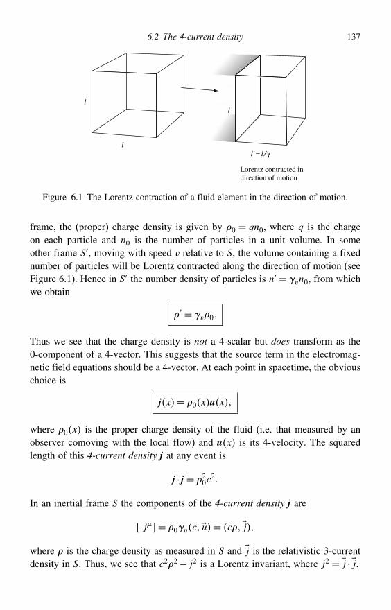
6.2 The 4-current density 137
l
Lorentz contracted indirection of motion
l'= l /γ
l
l
Figure 6.1 The Lorentz contraction of a fluid element in the direction of motion.
frame, the (proper) charge density is given by 0 = qn0, where q is the chargeon each particle and n0 is the number of particles in a unit volume. In someother frame S′, moving with speed v relative to S, the volume containing a fixednumber of particles will be Lorentz contracted along the direction of motion (seeFigure 6.1). Hence in S′ the number density of particles is n′ = vn0, from whichwe obtain
′ = v0
Thus we see that the charge density is not a 4-scalar but does transform as the0-component of a 4-vector. This suggests that the source term in the electromag-netic field equations should be a 4-vector. At each point in spacetime, the obviouschoice is
jx= 0xux
where 0x is the proper charge density of the fluid (i.e. that measured by anobserver comoving with the local flow) and ux is its 4-velocity. The squaredlength of this 4-current density j at any event is
j · j = 20c2
In an inertial frame S the components of the 4-current density j are
j= 0uc u= cj
where is the charge density as measured in S and j is the relativistic 3-currentdensity in S. Thus, we see that c22− j2 is a Lorentz invariant, where j2 = j · j.
138 Electromagnetism
6.3 The electromagnetic field equations
We are now in a position to write down the electromagnetic field equations. Thesimplest way in which to relate the rank-2 electromagnetic field tensor F to the4-vector j is to contract F with some other 4-vector. Since there are no morephysical 4-vectors associated with the theory, the only other 4-vector that the fieldequations can contain is the 4-gradient . Thus the field equations must be of theform
·F = kj (6.2)
where k is an unimportant constant related to our choice of units. In order to makeour final results more familiar, let us work in Cartesian inertial coordinates x
corresponding to some inertial frame S. In such a system, the covariant derivativereduces simply to the partial derivative, and so we can write (6.2) in componentform as
F = kj (6.3)
We can use this field equation to obtain the law for the conservation of charge.If we take the partial derivative of (6.3), we obtain
F = kj
(6.4)
However, since F is antisymmetric, we can write the scalar on the left-handside as
F =−F =−F =−F
from which we deduce that F = 0. Thus the right-hand side of (6.4) must
also be zero, so that
j = 0
Using 3-vector notation in the frame S, we may write this in a more familiar way:
t+ · j = 0
which expresses the conservation of charge. This equation has the same form asthe non-relativistic equation of charge continuity, but the relativistic expressionsfor and j must be used in it.
It is clear, however, that we do not yet have a viable theory. The field equationsof the theory are given by (6.3), but there are six independent components inF and only four field equations. Evidently our theory is under-determined as it
6.4 Electromagnetism in the Lorenz gauge 139
stands. This suggests that F could be constructed from a 4-vector ‘potential’ A.Again working in Cartesian inertial coordinates x, let us write
F = A− A (6.5)
Thus F is antisymmetric by construction and contains only four independentfields A. Using the field equation (6.3), we can write
kj = kj = F
= #F#
where we have used the fact that the metric coefficients in Cartesian inertialcoordinates x are constants.1 Hence, by substituting into the expression (6.5),we obtain the electromagnetic field equations in terms of the 4-vector potential Aas
##A− A#= kj (6.6)
Alternatively, we can express electromagnetism entirely in terms of the electro-magnetic field tensor F. In this case, we require the two field equations
F = kj
#F+ F#+ F# = 0(6.7)
where the second of these is straightforwardly derived from (6.5). Using theantisymmetrisation operation described in Section 4.3, the second equation canalso be written very succinctly as #F = 0. The constant k may be found bydemanding consistency with the standard Maxwell equations (see Section 6.5). InSI units we have k= 0, where 00 = 1/c2.
6.4 Electromagnetism in the Lorenz gauge
Suppose that we add an arbitrary 4-vector Q to the 4-potential A. Thus, incomponent form (in Cartesian inertial coordinates, x, for example) we have
Anew = A+Q (6.8)
Note that this is not a coordinate transformation. We are still working in the sameset of coordinates x but have defined a new vector Anew, whose components
1 In fact, such an operation is valid in any coordinate system. As we showed in Chapter 4, the covariantderivative of the metric tensor is identically zero, which means that we can interchange the order of indexraising or lowering and covariant differentiation without affecting the result.
140 Electromagnetism
in this basis are given by (6.8). The new electromagnetic field tensor is thengiven by
Fnew = A
new − A
new = A− A+ Q− Q
Clearly, we will recover the original electromagnetic field tensor provided that
Q = Q
This equation can be satisfied if Q is the gradient of some scalar field (say), sothat Q = . Thus we have uncovered a gauge freedom in the theory: we arefree to add the gradient of any scalar field to the 4-vector potential A, giving
Anew = A+ (6.9)
and still recover the same electromagnetic field tensor and hence the same elec-tromagnetic field equations. The transformation (6.9) is an example of a gaugetransformation and, as stated above, is distinct from a coordinate transformation.
In the field equations
##A− A#= 0j
the second term on the left-hand side can be written as A. Thus, we can
make this term zero by choosing a scalar field such that
A = 0 (6.10)
This condition is called the Lorenz gauge. It is worth noting that the condition(6.10) is preserved by any further gauge transformation A → A+ if andonly if
= 0.Adopting the Lorenz gauge allows the electromagnetic field equations to be
written very simply as
##A = A = 0j
It is usual to write the four-dimensional Laplacian using the notation 2 =
= , where 2 is the d’Alembertian operator.2 In Cartesian inertial
coordinates ct x y z,
2 = 1c2
2
t2− 2
x2− 2
y2− 2
z2
2 This operator should properly be written 2, which is the inner product · of the 4-gradient with itself.However, the notation we have adopted is quite common, since it makes clearer the distinction between thefour-dimensional Laplacian and the three-dimensional Laplacian 2 = · .
6.5 Electric and magnetic fields in inertial frames 141
Then the electromagnetic field equations in the Lorenz gauge take the especiallysimple form
2A = 0j
together with the attendant gauge condition (6.10). Moreover, in the absence ofcharges and currents, the right-hand side becomes zero and so A has wavesolutions travelling at the speed of light, as do the components of F since inthis case we also have 2F = 0.
6.5 Electric and magnetic fields in inertial frames
We have not yet identified the components of F (or A) with the familiar electricand magnetic 3-vector fields E and B as observed in some Cartesian inertial frameS. This is simply a matter of convention; we just have to name the components ofA (say) in a way which results in 3-vector equations in S that describe the physicscorrectly in terms of the traditionally defined 3-vectors E and B. Thus, in someCartesian inertial frame S, the components of A are taken to be as follows:
A=(
c A)
where is the electrostatic potential and A is the traditional three-dimensionalvector potential. In terms of and A, the Lorenz gauge condition becomes
· A+ 1c
t= 0
and, in this gauge, the field equations take the form
2 A= 0j and 2=
0
In terms of and A, the electric and magnetic fields in S are given by
B = × A and E =−− At
(6.11)
It is straightforward to show that these equations lead to the Maxwell equationsin their familiar form,
· E =
0
· B = 0
× E =−Bt
× B = 0j+00
Et
142 Electromagnetism
From the expressions (6.11) and (6.5) we have
Ei =−ijj− c0Ai =−cijjA0− 0Aj=−cijFj0
where we have used the fact that A0 = 0A = A0. Also, we have
B1 = 2A3− 3A
2 = 3A2− 2A3 = F32
where we have used the fact that Ai = iA =−Ai. Similar results hold for B2
and B3. Thus we find that the covariant components of F in S are given by
F=
⎛⎜⎜⎜⎝0 E1/c E2/c E3/c
−E1/c 0 −B3 B2
−E2/c B3 0 −B1
−E3/c −B2 B1 0
⎞⎟⎟⎟⎠
The corresponding electric and magnetic fields E′ and B′ in some other Cartesianinertial frame S′ are most easily obtained by calculating the components of theelectromagnetic field tensor F or the 4-potential A in this frame. For example, if S′is moving at speed v relative to S in standard configuration then the componentsin S′ are given by
A′ =$A
and F ′ =$#$
F
#
where the matrix $ is given in Chapter 5.
6.6 Electromagnetism in arbitrary coordinates
So far we have developed electromagnetic theory in Cartesian inertial coordinates.In general, however, we are free to label points in the Minkowski spacetime usingany arbitrary coordinate system x. We could have developed the entire theoryin such an arbitrary system, or even in a coordinate-independent way by usingthe 4-tensors themselves rather than their components in some coordinate system.Nevertheless, having expressed the theory in Cartesian inertial coordinates, it isnow trivial to re-express it in a form valid in arbitrary coordinates.
As shown in (6.7), the electromagnetic field equations in Cartesian inertialcoordinates, when expressed in terms of F, are given by
F = 0j
#F+ F#+ F# = 0
6.6 Electromagnetism in arbitrary coordinates 143
In such a coordinate system, the partial derivative is identical to the covariantderivative , so we can rewrite these equations as
F = 0j
#F+F#+F# = 0(6.12)
These new equations are now fully covariant tensor equations, however, so that ifthey are valid in one system of coordinates then they are valid in all coordinatesystems. Thus, (6.12) gives the electromagnetic field equations in an arbitrarycoordinate system! Once again, using the antisymmetrisation operation discussedin Section 4.3, one can write the second equation simply as #F = 0.A similar procedure can be performed for the electromagnetic field equations
when expressed in terms of the 4-vector potential A. From (6.6), in Cartesianinertial coordinates we have
##A− A#= 0j
Once again, we can replace by , but in this case we must also replace #
by g# , to obtain
g##A−A#= 0j
Again we have a fully covariant tensor equation, which must therefore be validin any arbitrary coordinate system, the metric coefficients of which are g# .In arbitrary coordinates, the electromagnetic field equations still permit the
gauge transformation
Anew = A+ = A+
where the last equality holds because the covariant derivative of the scalar field is simply its partial derivative. We can again choose a scalar field , so that
A = 0
which is the Lorenz gauge condition in arbitrary coordinates. In this case theelectromagnetic field equations can again be written in the form
2A = 0j
144 Electromagnetism
but now the d’Alembertian operator is given by 2= g = . In vacuo,we may again write 2A = 0 and 2F = 0. Also, charge conservation is givenin arbitrary coordinates by
j = 0
Finally, we note that the components of F and A in two different arbitrarycoordinate systems x and x′ are related by
A′ = x′
xA and F ′ = x′
x#x′
xF#
6.7 Equation of motion for a charged particle
From our original considerations in Section 6.1, we see that the coordinate-invariant manner of writing the equation of motion of a charged particle in anelectromagnetic field is
dpd=m0
dud= qF ·u
where m0 is the rest mass of the particle, p is its 4-momentum, u is its 4-velocityand is the proper time measured along its worldline. Note that the first equalityholds because the electromagnetic force is a pure force.
In Cartesian inertial coordinates, this becomes
m0du
d= qF
u
In a general coordinate system, however, the left-hand side is no longer validsince the ordinary derivative of the components of the 4-velocity along the parti-cle’s worldline must be replaced by the intrinsic derivative along the worldline.Using the expression for the intrinsic derivative given in Chapter 3, we findthat in an arbitary coordinate system the equation of motion of a particle in anelectromagnetic field is
m0Du
D=m0
(du
d+
#uu#
)= qF
u
where we have written dx#/d as u# since the 4-velocity is the tangent to theparticle’s worldline x.The equation for the particle’s worldline in arbitrary coordinates is thus given by
d2x
d2+
#
dx
d
dx#
d= q
m0F
dx
d (6.13)
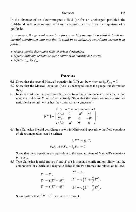
Exercises 145
In the absence of an electromagnetic field (or for an uncharged particle), theright-hand side is zero and we can recognise the result as the equation of ageodesic.
In summary, the general procedure for converting an equation valid in Cartesianinertial coordinates into one that is valid in an arbitrary coordinate system is asfollows:
• replace partial derivatives with covariant derivatives;• replace ordinary derivatives along curves with intrinsic derivatives;• replace by g.
Exercises
6.1 Show that the second Maxwell equation in (6.7) can be written as #F = 0.6.2 Show that the Maxwell equation (6.6) is unchanged under the gauge transformation
(6.9).6.3 In some Cartesian inertial frame S, the contravariant components of the electric and
magnetic fields are Ei and Bi respectively. Show that the corresponding electromag-netic field-strength tensor has the contravariant components
F=
⎛⎜⎜⎜⎝0 −E1/c −E2/c −E3/c
E1/c 0 −B3 B2
E2/c B3 0 −B1
E3/c −B2 B1 0
⎞⎟⎟⎟⎠
6.4 In a Cartesian inertial coordinate system in Minkowski spacetime the field equationsof electromagnetism can be written
F = 0j
#F+ F#+ F# = 0
Show that these equations are equivalent to the standard form of Maxwell’s equationsin vacuo.
6.5 Two Cartesian inertial frames S and S′ are in standard configuration. Show that thecomponents of electric and magnetic fields in the two frames are related as follows:
E′1 = E1
E′2 = E2−vB3
E′3 = E3+vB2
B′1 = B1
B′2 = (B2+ v
c2E3)
B′3 = (B3− v
c2E2)
Show further that c2 B2− E2 is Lorentz invariant.
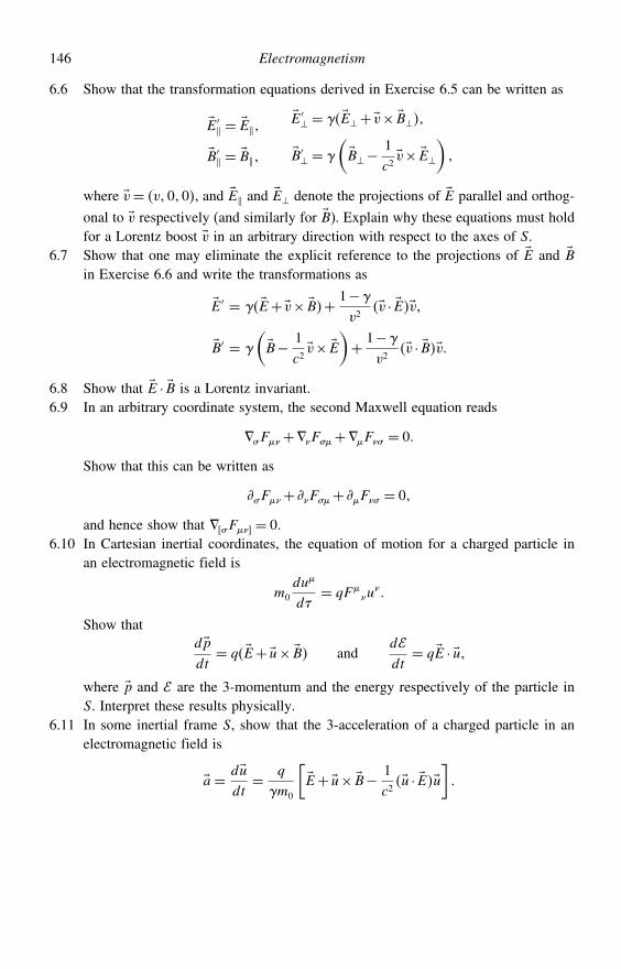
146 Electromagnetism
6.6 Show that the transformation equations derived in Exercise 6.5 can be written as
E′ = EB′ = B
E′⊥ = E⊥+v× B⊥
B′⊥ =
(B⊥−
1c2v× E⊥
)
where v= v00, and E and E⊥ denote the projections of E parallel and orthog-
onal to v respectively (and similarly for B). Explain why these equations must holdfor a Lorentz boost v in an arbitrary direction with respect to the axes of S.
6.7 Show that one may eliminate the explicit reference to the projections of E and Bin Exercise 6.6 and write the transformations as
E′ = E+v× B+ 1−
v2v · Ev
B′ =
(B− 1
c2v× E
)+ 1−
v2v · Bv
6.8 Show that E · B is a Lorentz invariant.6.9 In an arbitrary coordinate system, the second Maxwell equation reads
#F+F#+F# = 0
Show that this can be written as
#F+ F#+ F# = 0
and hence show that #F = 0.6.10 In Cartesian inertial coordinates, the equation of motion for a charged particle in
an electromagnetic field is
m0
du
d= qF
u
Show thatdpdt= qE+ u× B and
d
dt= q E · u
where p and are the 3-momentum and the energy respectively of the particle inS. Interpret these results physically.
6.11 In some inertial frame S, show that the 3-acceleration of a charged particle in anelectromagnetic field is
a= dudt= q
m0
[E+ u× B− 1
c2u · Eu
]
7
The equivalence principle and spacetime curvature
We are now in a position to use the experience gained in deriving a relativisticformulation of electromagnetism (together with some flashes of inspiration fromEinstein!) to begin our formulation of a relativistic theory of gravity, namelygeneral relativity.
7.1 Newtonian gravity
In our development of electromagnetism, we began by considering the electro-magnetic 3-force on a charged particle. Let us therefore start our discussion ofgravity by considering the description of the gravitational force in the classical,non-relativistic, theory of Newton. In the Newtonian theory, the gravitationalforce f on a (test) particle of gravitational mass mG at some position is
f =mGg =−mG%
where g is the gravitational field derived from the gravitational potential % at thatposition. In turn, the gravitational potential is determined by Poisson’s equation:
2% = 4G (7.1)
where is the gravitational matter density and G is Newton’s gravitationalconstant. This is the field equation of Newtonian gravity.
It is clear from (7.1) that Newtonian gravity is not consistent with specialrelativity. There is no explicit time dependence, which means that the potential% (and hence the gravitational force on a particle) responds instantaneously to adisturbance in the matter density ; this violates the special-relativistic requirementthat signals cannot propagate faster than c. We might try to remedy this by noting
147
148 The equivalence principle and spacetime curvature
that the Laplacian operator 2 in (7.1) is equivalent to minus the d’Alembertianoperator 2 in the limit c→, and thus postulate the modified field equation
2% =−4G
However, this equation does not yield a consistent relativistic theory. It is stillnot Lorentz covariant, since the matter density does not transform as a Lorentzscalar. We shall discuss the transformation properties of the matter density later.
In addition to the incompatibility of Newtonian gravity with special relativity,there is a second fundamental difference between the electromagnetic and grav-itational forces. The equation of motion of a particle of inertial mass mI in agravitational field is given by
d2xdt2
=−mG
mI
% (7.2)
It is a well-established experimental fact, however, that the ratiomG/mI appearingin the equation of motion is the same for all particles. By an appropriate choice ofunits one may thus arrange for this ratio to equal unity. In contrast, the ratio q/mI
occurring in the equation of motion of a charged particle in an electromagneticfield is not the same for all particles. From (7.2), we thus see that the trajectorythrough space of a particle in a gravitational field is independent of the nature ofthe particle.
This equivalence of the gravitational and inertial masses (which allows us torefer simply to ‘the mass’), is a truly remarkable coincidence in the Newtoniantheory. In this theory, there is no a-priori reason why the quantity that determinesthe magnitude of the gravitational force on the particle should equal the quantitythat determines the particle’s ‘resistance’ to an applied force in general. It appearsas an isolated experimental result, which has since been verified to an accuracyof at least one part in 1011 (by Dicke and co-workers).
7.2 The equivalence principle
The equality of the gravitational and inertial masses of a particle led Einsteinto his classic ‘elevator’ thought experiment. Consider an observer in a freelyfalling elevator (i.e. after the lift cable has been cut). Objects released fromrest relative to the elevator cabin remain floating ‘weightless’ in the cabin.A projectile shot from one side of the elevator to the other appears to movein a straight line at constant velocity, rather than in the usual curved trajectory.All this follows from the fact that the acceleration of any particle relative to
7.3 Gravity as spacetime curvature 149
the elevator is zero: the particle and the elevator cabin have the same accelera-tion relative to the Earth as a result of the equivalence of gravitational and inertialmass.
All these observations would hold exactly if the gravitational field of the Earthwere truly uniform. Of course, the gravitational field of the Earth is not uniformbut acts radially inwards towards its centre of mass, with a strength proportionalto 1/r2. Thus, if the elevator were left to free-fall for a long time or if it were verylarge (i.e. a significant fraction of the Earth’s radius), two particles released fromrest near the walls of the elevator would gradually drift inwards, since they wouldboth be falling along radial lines towards the centre of the Earth (see Figure 7.1).Furthermore, as a result of the varying strength of the gravitational field, particlesreleased from rest near the floor of the elevator would gradually drift downwardswhereas those near the ceiling would drift upwards. What the observer in theelevator would be experiencing would be the tidal forces resulting from theresidual inhomogeneity in the strength and direction of the gravitational field oncethe main acceleration has been subtracted. It should always be remembered thatthese tidal forces can never be completely abolished in an elevator (laboratory)of finite, i.e. non-zero, size.
Nevertheless, provided that we consider the elevator cabin over a short timeperiod and that it is spatially small, then a freely falling elevator (which mayhave x y z coordinates marked on its walls and an elevator clock measuringtime t) resembles a Cartesian inertial frame of reference, and therefore the lawsof special relativity hold inside the elevator.1 These observations lead to
The equivalence principle: In a freely falling (non-rotating) laboratory occupyinga small region of spacetime, the laws of physics are those of special relativity.2
7.3 Gravity as spacetime curvature
These observations led Einstein to make a profound proposal that simultaneouslyprovides for a relativistic description of gravity and incorporates in a natural waythe equivalence principle (and consequently the equivalence of gravitational andinertial mass). Einstein’s proposal was that gravity should no longer be regardedas a force in the conventional sense but rather as a manifestation of the curvatureof the spacetime, this curvature being induced by the presence of matter. This isthe central idea underpinning the theory of general relativity.
1 The elevator cabin must not only occupy a small region of spacetime but also be non-rotating with respect todistant matter in the universe. This statement is related to Mach’s principle.
2 This is in fact a statement of the strong equivalence principle, since it refers to all the Laws of physics. Themore modest weak equivalence principle refers only to the trajectories of freely falling particles.
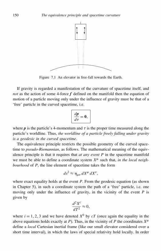
150 The equivalence principle and spacetime curvature
Figure 7.1 An elevator in free-fall towards the Earth.
If gravity is regarded a manifestation of the curvature of spacetime itself, andnot as the action of some 4-force f defined on the manifold then the equation ofmotion of a particle moving only under the influence of gravity must be that of a‘free’ particle in the curved spacetime, i.e.
dpd= 0
where p is the particle’s 4-momentum and is the proper time measured along theparticle’s worldline. Thus, the worldline of a particle freely falling under gravityis a geodesic in the curved spacetime.
The equivalence principle restricts the possible geometry of the curved space-time to pseudo-Riemannian, as follows. The mathematical meaning of the equiv-alence principle is that it requires that at any event P in the spacetime manifoldwe must be able to define a coordinate system X such that, in the local neigh-bourhood of P, the line element of spacetime takes the form
ds2 ≈ dX dX
where exact equality holds at the event P. From the geodesic equation (as shownin Chapter 5), in such a coordinate system the path of a ‘free’ particle, i.e. onemoving only under the influence of gravity, in the vicinity of the event P isgiven by
d2Xi
dT 2≈ 0
where i = 123 and we have denoted X0 by cT (once again the equality in theabove equations holds exactly at P). Thus, in the vicinity of P the coordinates X
define a local Cartesian inertial frame (like our small elevator considered over ashort time interval), in which the laws of special relativity hold locally. In order
7.4 Local inertial coordinates 151
that we can construct such a system, spacetime must be a pseudo-Riemannianmanifold (which is curved and four-dimensional). For such a manifold, in somearbitrary coordinate system x the line element takes the general form
ds2 = g dx dx
7.4 Local inertial coordinates
The curvature of spacetime means that it is not possible to find coordinates inwhich the metric g = at all points in the manifold. Thus, it is not possibleto define global Cartesian inertial frames as we could in the pseudo-EuclideanMinkowski spacetime. Instead, we are forced to use arbitrary coordinate systemsx to label events in spacetime, and these coordinates often do not have simplephysical meanings. It is often the case that x0 is a timelike coordinate and thexii = 123 are spacelike (i.e. the tangent vector to the x0 coordinate curve istimelike at all points, and similarly the tangent vectors to the xi coordinate curvesare always spacelike). This allocation of coordinates is not necessary, however,and it is sometimes useful to define null coordinates. In any case, the arbitrarycoordinates x need not have any direct physical interpretation.
Nevertheless, as demanded by the equivalence principle, problems of physicalmeaning can always be overcome by transforming, at any event P in the curvedspacetime, to a local inertial coordinate system X, which, in a limited region ofspacetime about P, corresponds to a freely falling, non-rotating, Cartesian frameover a short time interval. Mathematically, this corresponds to constructing aboutthe event P a coordinate system X such that
gP= and #gP = 0 (7.3)
This also means that #P = 0 and that the coordinate basis vectors at the
event P form an orthonormal set, i.e.
eP · eP= (7.4)
There are in fact an infinite number of local inertial coordinate systems at P, allof which are related to one another by Lorentz transformations. In other words,if a coordinate system X satisfies the conditions (7.3), and hence the condition(7.4), then so too will the coordinate system
X′ =$X
where $ defines a Lorentz transformation. Thus, local Cartesian freely falling
(non-rotating) frames at an event P are related to one another by boosts, spatial
152 The equivalence principle and spacetime curvature
rotations or combinations of the two. For any one of these coordinate systems, thetimelike basis vector e0P is simply the normalised 4-velocity vector uP of theorigin of that frame at the event P, and the three mutually orthogonal spacelikevectors eiPi= 123 define the orientation of the spatial axes of the frame.
For points near to P, the metric in a local inertial coordinate system X (whoseorigin is at P) is given by
g = + 12#gPX
#X+· · · The sizes of the second derivatives #gP thus determine the region overwhich the approximation g ≈ remains valid. We shall see the significanceof these second derivatives shortly.
7.5 Observers in a curved spacetime
We discussed the subject of observers in Minkowski spacetime in Chapter 5, butlet us now consider the subject in its full generality, in a curved spacetime. Anobserver will trace out some general (timelike) worldline x through spacetime,as expressed in some arbitrary coordinate system, where is the observer’s propertime. An idealisation of his local laboratory is a frame of four orthonormal vectorse (or tetrad) satisfying
e · e=
which are carried with him along his worldline (these vectors may, in general,be totally unrelated to the basis vectors e of the coordinate system that we areusing to label points in spacetime, although we can always express one set ofvectors in terms of the other). In particular, at any point along his worldline thetimelike vector e0 coincides with the normalised 4-velocity u = u/c ofthe observer. Similarly, the evolution of the spacelike vectors ei along theworldline reflect the different ways in which his local laboratory may be spinningor tumbling. Quantities measured in this laboratory correspond to projections ofthe relevant physical 4-vectors and 4-tensors onto this orthonormal frame.
As shown in Chapter 5, if the observer has a 4-acceleration a= du/d butis not rotating, the tetrad basis vectors are Fermi–Walker-transported along theobserver’s worldline:
ded
= 1c2[u · ea− a · eu
] (7.5)
This expression holds equally well in a curved spacetime. An important specialcase is that of a non-rotating, freely falling observer, i.e one who is moving only
7.6 Weak gravitational fields and the Newtonian limit 153
under the influence of gravity. The vectors e then define what is called afreely falling frame (FFF). Free from any external forces, the observer’s worldlinetraces out a geodesic in the curved spacetime. Thus the timelike vector e0 changeswith proper time along the worldline according to
de0d
= 0
In other words, e0 is parallel-transported along the worldline, and the observer’s4-acceleration a is zero. In this case we see from (7.5) that Fermi–Walker transportreduces to parallel transport. Thus the spacelike frame vectors ei (i= 123) arealso parallel-transported along the geodesic, so that
deid
= 0
Hence, in an arbitrary coordinate system x, the components e= e ·e
of any frame vector evolve as follows:
De
D= de
d+
#eu# = 0
This equation is extremely useful for determining what a freely falling observerwould measure at a given event in spacetime. It is also clear that the frame vectorse at any event P along the observer’s worldline are the basis vectors of a localCartesian inertial coordinate system at P.
7.6 Weak gravitational fields and the Newtonian limit
It is clear that, by construction, our description of gravity in terms of spacetimecurvature reduces to special relativity in local inertial frames. It is important tocheck, however, that such a description also reduces to Newtonian gravity in theappropriate limits.
In the absence of gravity, spacetime has a Minkowski geometry. Therefore aweak gravitational field corresponds to a region of spacetime that is only ‘slightly’curved. In other words, in such a region there exist coordinates x in which themetric takes the form
g = +h where h 1 (7.6)
Note that it is important to say ‘there exist coordinates’ since (7.6) does not holdfor all coordinates; as we saw in Chapter 5, one can find coordinates even inMinkowski space in which g is not close to the simple form . Let us assumethat in the coordinate system (7.6) the metric is stationary, which means that all
154 The equivalence principle and spacetime curvature
the derivatives 0g are zero. An example of such a coordinate system might bea fixed Cartesian frame at some point on the surface of the (non-rotating) Earth.
The worldline of a particle freely falling under gravity is given in general bythe geodesic equation
d2x
d2+
#
dx
d
dx#
d= 0
We shall assume, however, that the particle is slow-moving, so that the compo-nents of its 3-velocity satisfy dxi/dt ci = 123, where t is defined byx0 ≡ ct. This is equivalent to demanding that, for i= 123,
dxi
d dx0
d
Thus we can ignore the 3-velocity terms in the geodesic equation to obtain
d2x
d2+
00c2(dt
d
)2
= 0 (7.7)
Now, recalling the expression (3.21) giving the connection in terms of the metricand using the form (7.6) for g, we find that the connection coefficients
00
are given by
00 = 1
2g&0g0&+ 0g0&− &g00=− 1
2g&&g00 =− 1
2&&h00
where the last equality is valid to first order in h. Since we have assumed thatthe metric is stationary, we have
000 = 0 and i
00 = 12
ijjh00
where the Latin index runs over i= 123. Inserting these coefficients into (7.7)gives
d2t
d2= 0 and
d2xd2
=− 12c
2(dt
d
)2h00
The first equation implies that dt/d = constant, and so we can combine the twoequations to yield the following equation of motion for the particle:
d2xdt2=− 1
2c2 h00
If we compare this equation with the usual Newtonian equation of motion fora particle in a gravitational field (7.2), we see that the two are identical if wemake the indentification h00 = 2%/c2. Hence for a slowly moving particle our
7.7 Electromagnetism in a curved spacetime 155
description of gravity as spacetime curvature tends to the Newtonian theory if themetric is such that, in the limit of a weak gravitational field,
g00 =(1+ 2%
c2
) (7.8)
How big is the correction to the Minkowski metric? Some values of %/c2 forvarious systems are as follows:
%
c2=−GM
c2r=
⎧⎪⎨⎪⎩−10−9 at the surface of the Earth
−10−6 at the surface of the Sun
−10−4 at the surface of a white dwarf star
Thus, we see that even at the surface of a dense object like a white dwarf, thesize of %/c2 is much smaller than unity and hence the weak-field limit will bean excellent approximation.
From (7.8), the observant reader will have noticed that the description of gravityin terms of spacetime curvature has another immediate consequence, namely thatthe time coordinate t does not, in general, measure proper time. If we consider aclock at rest at some point in our coordinate system (i.e. dxi/dt = 0), the propertime interval d between two ‘clicks’ of the clock is given by
c2d2 = g dx dx = g00c
2 dt2
from which we find that
d =(1+ 2%
c2
)1/2
dt
This gives the interval of proper d corresponding to an interval dt of coordinatetime for a stationary observer near a massive object, in a region where thegravitational potential is%. Since% is negative, this proper time interval is shorterthan the corresponding interval for a stationary observer at a large distance fromthe object, where %→ 0 and so d = dt. Thus, as a bonus, our analysis has alsoyielded the formula for time dilation in a weak gravitational field.
7.7 Electromagnetism in a curved spacetime
Before going on to discuss the mathematics of curvature in detail, let us lookback at our development of electromagnetism in Chapter 6. It is clear that ourderivation of the electromagnetic field equations in arbitrary coordinates did not
156 The equivalence principle and spacetime curvature
depend on the intrinsic geometry of the manifold on which the electromagneticfield tensor F and the 4-current j are defined. In other words, one can arrive atthese equations without assuming the spacetime to have a Minkowski geometry.Thus, in the presence of gravitating matter, spacetime becomes curved but thefield equations of electromagnetism in an arbitrary coordinate system are stillgiven by
F = 0j
#F+F#+F# = 0(7.9)
The effects of gravitation are automatically included in these field equationsthrough the covariant derivatives, which depend on the metric g describingthe spacetime geometry. Moreover, if we construct a local Cartesian coordinatesystem about some point P in the manifold then (as discussed above) thesecoordinates correspond to a local inertial frame in the neighbourhood of P. In thesecoordinates, the equations of electromagnetism then take their familiar specialrelativistic forms.
An electromagnetic field tensor F defined on a curved spacetime gives rise (asin Minkowski space) to a 4-force f = qF ·u, which acts on a particle of chargeq with 4-velocity u. Thus the equation of motion of a charged particle movingunder the influence of an electromagnetic field in a curved spacetime has thesame form as that in Minkowski spacetime, i.e.
m0dud= qF ·u
where m0 is the rest mass of the particle. In this case, however, because ofthe curvature of spacetime the particle is moving under the influence of bothelectromagnetic forces and gravity. In some arbitrary coordinate system, theparticle’s worldline is again given by
d2x
d2+
#
dx
d
dx#
d= q
m0F
dx
d
Obviously, in the absence of an electromagnetic field (or for an uncharged parti-cle), the right-hand side is zero and we recover the equation of a geodesic.
We must remember, however, that the energy and momentum of the electro-magnetic field will itself induce a curvature of spacetime, so the metric in thiscase is determined not only by the matter distribution but also by the radiation.
7.8 Intrinsic curvature of a manifold 157
7.8 Intrinsic curvature of a manifold
Since the notion of curvature is central to general relativity, we must now inves-tigate how to quantify the intrinsic curvature of a manifold at any given point P.3
A manifold (or region of a manifold) is flat if there exist coordinates X suchthat, throughout the region, the line element can be written
ds2 = 1dX12+ 2dX
22+· · ·+ N dXN2 (7.10)
where a = ±1 (in other words ‘flat’ is a shorthand for pseudo-Euclidean). If,however, points in the manifold are labelled with some arbitrary coordinate systemxa then in general the line element ds2 will not be of the above form. Thus, if forsome manifold the line element is given by
ds2 = gabxdxa dxb
how can we tell whether the intrinsic geometry of the manifold in some region isflat or curved in some way?
Consider, for example, the following line element for a three-dimensional space:
ds2 = dr2+ r2d2+ r2 sin2 d2
Of course, we recognise this as the line element of ordinary three-dimensionalEuclidean space written in spherical polar coordinates. In other words, the trans-formation
x = r sin cos y = r sin sin z= r cos
will turn the above line element into the form
ds2 = dx2+dy2+dz2 (7.11)
But what about other line elements? For example, recall from Chapter 2 thethree-dimensional space described by the line element (2.21):
ds2 = a2
a2− r2dr2+ r2 d2+ r2 sin2 d2
How can we tell whether this metric, or a more complicated metric, correspondsto flat space but merely looks complicated because of a weird choice of coordi-nates? It would be immensely tedious to try to discover whether there exists acoordinate transformation that reduces a metric to the form (7.11). We thereforeneed some means of telling whether a manifold is flat directly from the metricgab, independently of the coordinate system being used.
3 Since the material presented here is applicable to any N -dimensional pseudo-Riemannian manifold, we willuse indices ab etc. that have a range 1 to N , rather than etc., with a range 0 to 3. Of course, the finalapplication to general relativity will govern the scope of our results.
158 The equivalence principle and spacetime curvature
The physical significance of this to general relativity is as follows. If, throughoutsome region of a four-dimensional spacetime, we can reduce the line element
ds2 = g dx dx
to Minkowski form then there can be no gravitational field in this region. Theequivalence of a general line element to that of Minkowski spacetime thereforeguarantees that the gravitational field will vanish. The solution to our mathematicalproblem of finding a coordinate-independent way of defining the curvature ofspacetime will lead us to the field equations of gravity.
7.9 The curvature tensor
We can find a solution to the problem of measuring the curvature of a manifold atany point by considering changing the order of covariant differentiation. Covariantdifferentiation is clearly a generalisation of partial differentiation. There is oneimportant respect in which it differs, however: it matters in which order covariantdifferentiation is performed, and changing the order (in general) changes the result.
Since for a scalar field the covariant derivative is simply the partial deriva-tive, the order of differentiation does not matter. However, let us consider somearbitrary vector field defined on a manifold, with covariant components va. Thecovariant derivative of the va is given by
bva = bva− dabvd
A second covariant differentiation then yields
cbva = cbva− eacbve− e
bceva
= cbva− c dabvd− d
abcvd
− eacbve− d
ebvd− ebceva− d
aevd
which follows since bva is itself a rank-2 tensor. Swapping the indices b and cto obtain a corresponding expression for bcva and then subtracting gives
cbva−bcva = Rdabcvd (7.12)
where
Rdabc ≡ b
dac− c
dab+ e
ac deb− e
ab dec (7.13)
To determine directly whether the N 4 quantities Rdabc transform as the compo-
nents of a tensor under a coordinate transformation would be an arduous algebraictask. Fortunately the quotient theorem (Section 4.11) provides a much shorterroute. The left-hand side of (7.12) is a tensor, for arbitrary vectors va, so the
7.10 Properties of the curvature tensor 159
contraction of Rdabc with vd is also a tensor. Since Rd
abc does not depend on va,we conclude from the quotient theorem that the Rd
abc are indeed the componentsof some rank-4 tensor R. This tensor is called the curvature tensor (or Riemanntensor), and equation (7.13) shows that it is defined in terms of the metric tensorgab and its first and second derivatives.
We must now establish how the tensor (7.13) is related to the curvature of themanifold. In a flat region of a manifold, we may choose coordinates such thatthe line element takes the form (7.10) throughout the region. In these coordinates a
bc and its derivatives are zero, and hence
Rdabc = 0
at every point in the region. This is a tensor relation, however, and so it must holdin any coordinate system. Conversely, if Rd
abc = 0 at every point in some regionof a manifold, then it may be shown that it is possible to introduce a coordinatesystem in which the line element takes the form (7.10), and hence this regionis flat.4 Thus the vanishing of the curvature tensor is a necessary and sufficientcondition for a region of a manifold to be flat.
7.10 Properties of the curvature tensor
The curvature tensor (7.13) possesses a number of symmetries and satisfies certainidentities, which we now discuss. The symmetries of the curvature tensor are mosteasily derived in terms of its covariant components
Rabcd = gaeRebcd
For completeness, we note that in an arbitrary coordinate system an explicit formfor these components is found, after considerable algebra, to be
Rabcd = 12dagbc− dbgac+ cbgad− cagbd−gef eac fbd− ead fbc
One could use this expression straightforwardly to derive the symmetry propertiesof the curvature tensor, but we take the opportunity here to illustrate a generalmathematical device that is often useful in reducing the algebraic burden of tensormanipulations.
Let us choose some arbitrary point P in the manifold and construct a geodesiccoordinate system about this point (see Section 3.11), in which the connec-tion vanishes, a
bcP = 0, although in general its derivatives will not. In this
4 For a proof of this result, see (for example) P. A. M. Dirac, General Theory of Relativity, Princeton Landmarksin Physics Series, Princeton University Press, 1996.
160 The equivalence principle and spacetime curvature
coordinate system, one may easily show directly from (7.13) that the covariantcomponents of the curvature tensor at P are given by
RabcdP = 12dagbc− dbgac+ cbgad− cagbdP
From this expression one may immediately establish the following symmetryproperties at P:
Rabcd =−Rbacd
Rabcd =−Rabdc
Rabcd = Rcdab
(7.14)
(7.15)
(7.16)
The first two properties show that the curvature tensor is antisymmetric withrespect to swapping the order of either the first two indices or the second twoindices. The third property shows that it is symmetric with respect to swappingthe first pair of indices with the second pair of indices. Moreover, we may alsoeasily deduce the cyclic identity
Rabcd+Racdb+Radbc = 0 (7.17)
which on using (7.15) may be written more succinctly as Ra bcd = 0. Althoughthe results (7.14–7.17) have been derived in a special coordinate system, eachcondition is a tensor relation and so if it is valid in one coordinate system then it isvalid in all. Moreover, since the point P is arbitrary, the results hold everywhere.
Although first appearances might suggest that the curvature tensor has N 4
components, the conditions (7.14–7.17) reduce the number of independent compo-nents to N 2N 2−1/12. Recall from Section 2.11 that this is also the number ofdegrees of freedom among the second derivatives dcgab. This is not surprisingsince, at any point P in a manifold, we can perform a transformation to localCartesian coordinates in which gabP = and cgabP = 0. Thus, a generalmetric at any point P is characterised by the N 2N 2−1/12 second derivativesthat cannot be made to vanish there.
For manifolds of different dimensions we have the following results:
No. of dimensions 2 3 4No. of independent components of Rabcd 1 6 20
You can see from this table that in four dimensions the number of independentcomponents is reduced from a possible 256 to 20. You will also see that in onedimension the curvature tensor is always equal to zero: R1111 = 0. How can this
7.11 The Ricci tensor and curvature scalar 161
be? Can a line not be curved? Think about this – the curvature measures the‘inner’ properties of the space. When we say that a line is curved we refer toa particular embedding in a higher-dimensional space, but this does not tell usabout the inner properties of the space. In one dimension, it is evident that wecan always find a coordinate transformation that will reduce an arbitrary metric tothe form (7.10). As a two-dimensional example, in Appendix 7A we calculate thesingle independent component of the curvature tensor for the surface of a sphere.The Gaussian curvature K of a two-dimensional surface is given by
K = R1212
g
where g = det gab is the determinant of the metric tensor.The curvature tensor also satisfies a differential identity, which may be derived
as follows. Let us once again adopt a geodesic coordinate system about somearbitrary point P. In this coordinate system, differentiating and then evaluatingthe result at P gives
eRabcdP = eRabcdP = ec abd− ed abcP
Cyclically permuting c, d and e to obtain two further analogous relations andadding, one finds that at P
eRabcd+cRabde+dRabec = 0 (7.18)
This is, however, a tensor relation and thus holds in all coordinate systems;moreover, since P is arbitrary the relationship holds everywhere. This result isknown as the Bianchi identity and, using the antisymmetry relation (7.14), it maybe written more succinctly as
eRabcd = 0
7.11 The Ricci tensor and curvature scalar
It follows from the symmetry properties (7.14–7.16) of the curvature tensor thatit possesses only two independent contractions. We may find these by contractingeither on the first two indices or on the first and last indices respectively. From(7.14), raising the index a and then contracting on the first two indices gives
Raacd = 0
Contracting on the first and last indices, however, gives in general a non-zeroresult and this leads to a new tensor, the Ricci tensor. It is traditional to use the
162 The equivalence principle and spacetime curvature
same kernel letter for the Ricci tensor as for the curvature tensor, so we denoteits components by
Rab ≡ Rcabc
By raising the index a in the cyclic identity (7.17) and contracting with d, onemay easily show that the Ricci tensor is symmetric. Thus we have Ra
b =Rab and
we can denote both by Rba.
A further contraction gives the curvature scalar (or Ricci scalar)
R≡ gabRab = Raa
where again the same kernel letter is used. This is a scalar quantity defined ateach point of the manifold.
The covariant derivatives of the Ricci tensor and the curvature scalar obey aparticularly important relation, which will be central to our development of thefield equations of general relativity. Raising a in the Bianchi identity (7.18) andcontracting with d gives
eRbc+cRabae+aR
abec = 0
which, on using the antisymmetry property (7.16) in the second term, gives
eRbc−cRbe+aRabec = 0
If we now raise b and contract with e, we find
bRbc−cR+aR
abbc = 0 (7.19)
Using the antisymmetry properties (7.14, 7.15) we may write the third term as
aRab
bc = aRba
cb = aRac = bR
bc
so the first and last terms in (7.19) are identical and we obtain
2bRbc−cR= b
(2Rb
c−bcR)= 0
Finally, raising the index c, we obtain the important result
b
(Rbc− 1
2gbcR
)= 0
The term in parentheses is called the Einstein tensor
Gab ≡ Rab− 12g
abR
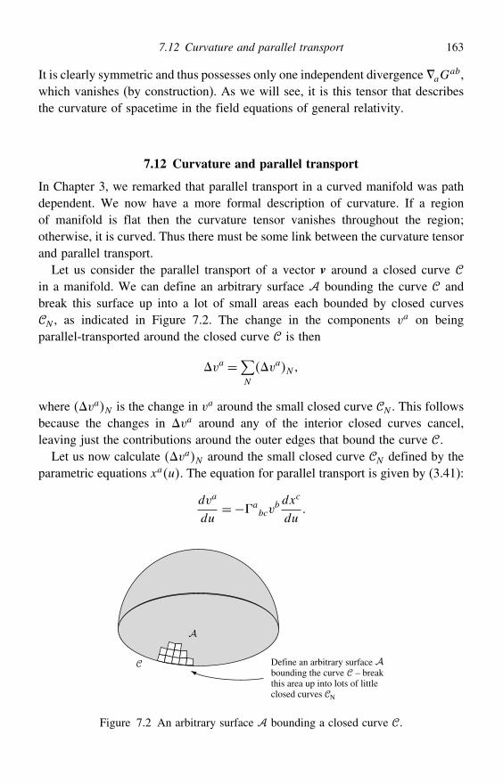
7.12 Curvature and parallel transport 163
It is clearly symmetric and thus possesses only one independent divergence aGab,
which vanishes (by construction). As we will see, it is this tensor that describesthe curvature of spacetime in the field equations of general relativity.
7.12 Curvature and parallel transport
In Chapter 3, we remarked that parallel transport in a curved manifold was pathdependent. We now have a more formal description of curvature. If a regionof manifold is flat then the curvature tensor vanishes throughout the region;otherwise, it is curved. Thus there must be some link between the curvature tensorand parallel transport.
Let us consider the parallel transport of a vector v around a closed curve in a manifold. We can define an arbitrary surface bounding the curve andbreak this surface up into a lot of small areas each bounded by closed curvesN , as indicated in Figure 7.2. The change in the components va on beingparallel-transported around the closed curve is then
va =∑N
vaN
where vaN is the change in va around the small closed curve N . This followsbecause the changes in va around any of the interior closed curves cancel,leaving just the contributions around the outer edges that bound the curve .
Let us now calculate vaN around the small closed curve N defined by theparametric equations xau. The equation for parallel transport is given by (3.41):
dva
du=− a
bcvb dx
c
du
Define an arbitrary surface bounding the curve – breakthis area up into lots of littleclosed curves N
Figure 7.2 An arbitrary surface bounding a closed curve .
164 The equivalence principle and spacetime curvature
Thus, if va is parallel-transported along the small closed curve N from someinitial point P then at some other point along this curve we have
vau= vaP−∫ u
uP
abcv
b dxc
dudu (7.20)
However, since the closed curve is small we can expand the factors in the integrandabout P to first order in xa−xaP :
abcu = a
bcP+ d abcP
[xdu−xdP
]+· · · vau = vaP− a
bcP vbP x
cu−xcP+· · · Substituting these expressions into (7.20) and retaining terms only up to first orderin xa−xaP , we obtain
vau = vaP− abcP v
bP
∫ u
uP
dxc
dudu
− d abc− a
ec ebdP v
bP
∫ u
uP
(xd−xdP
) dxcdu
du
If we integrate the coordinate differentials around a closed loop we have∮dxc= 0,
and so we find that
va =− d abc− a
ec ebdP v
bP
∮ u
uP
xd dxc
We may obtain an analogous result by interchanging the dummy indices c and d.Now using the result ∮
dxcxd=∮xc dxd+xd dxc= 0
we find that
va =− 12 c
abd− d
abc+ a
ec ebd− a
ed ebcP v
bP
∮xc dxd
On using the expression (7.13), we finally obtain
va =− 12 R
abcdP v
bP
∮xc dxd (7.21)
Equation (7.21) establishes the link between the curvature tensor at a pointP and parallel transport around a small loop close to P. It tells us that thecomponents va will remain unchanged after parallel transportation around a smallclosed loop near P if and only if the curvature tensor vanishes at P. So, returning
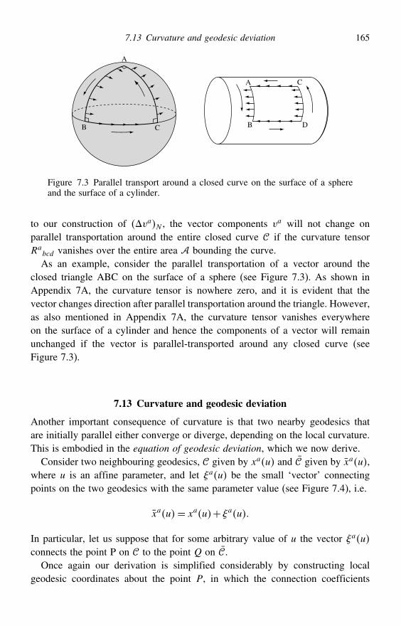
7.13 Curvature and geodesic deviation 165
A
B C
A
B
C
D
Figure 7.3 Parallel transport around a closed curve on the surface of a sphereand the surface of a cylinder.
to our construction of vaN , the vector components va will not change onparallel transportation around the entire closed curve if the curvature tensorRa
bcd vanishes over the entire area bounding the curve.As an example, consider the parallel transportation of a vector around the
closed triangle ABC on the surface of a sphere (see Figure 7.3). As shown inAppendix 7A, the curvature tensor is nowhere zero, and it is evident that thevector changes direction after parallel transportation around the triangle. However,as also mentioned in Appendix 7A, the curvature tensor vanishes everywhereon the surface of a cylinder and hence the components of a vector will remainunchanged if the vector is parallel-transported around any closed curve (seeFigure 7.3).
7.13 Curvature and geodesic deviation
Another important consequence of curvature is that two nearby geodesics thatare initially parallel either converge or diverge, depending on the local curvature.This is embodied in the equation of geodesic deviation, which we now derive.
Consider two neighbouring geodesics, given by xau and given by xau,where u is an affine parameter, and let au be the small ‘vector’ connectingpoints on the two geodesics with the same parameter value (see Figure 7.4), i.e.
xau= xau+au
In particular, let us suppose that for some arbitrary value of u the vector auconnects the point P on to the point Q on .
Once again our derivation is simplified considerably by constructing localgeodesic coordinates about the point P, in which the connection coefficients
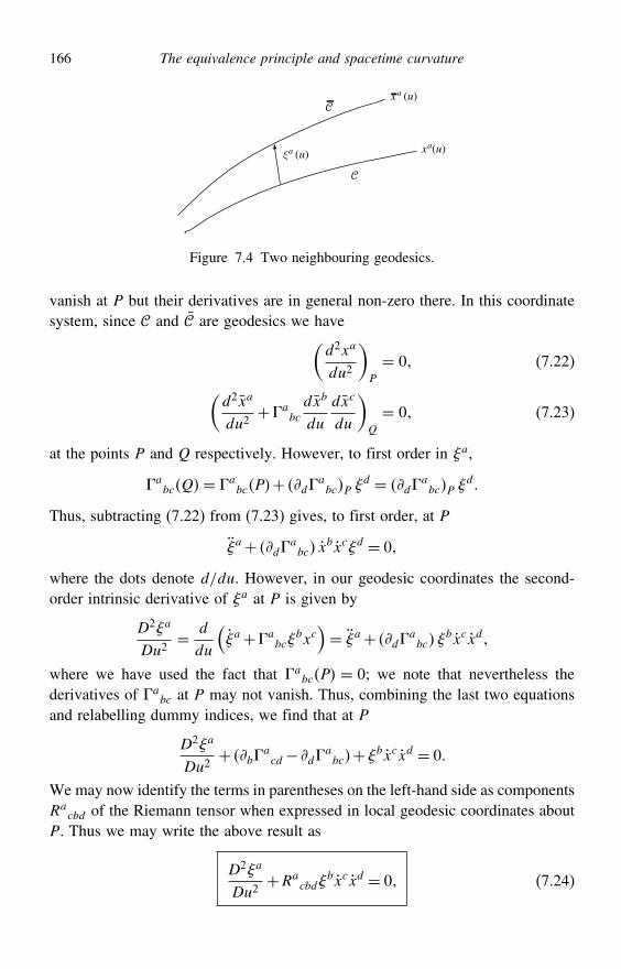
166 The equivalence principle and spacetime curvature
ξ a (u)
xa (u)
xa(u)
Figure 7.4 Two neighbouring geodesics.
vanish at P but their derivatives are in general non-zero there. In this coordinatesystem, since and are geodesics we have(
d2xa
du2
)P
= 0 (7.22)(d2xa
du2+ a
bc
dxb
du
dxc
du
)Q
= 0 (7.23)
at the points P and Q respectively. However, to first order in a,
abcQ= a
bcP+ d abcP
d = d abcP
d
Thus, subtracting (7.22) from (7.23) gives, to first order, at P
a+ d abc x
bxcd = 0
where the dots denote d/du. However, in our geodesic coordinates the second-order intrinsic derivative of a at P is given by
D2a
Du2= d
du
(a+ a
bcbxc)= a+ d
abc
bxcxd
where we have used the fact that abcP = 0; we note that nevertheless the
derivatives of abc at P may not vanish. Thus, combining the last two equations
and relabelling dummy indices, we find that at P
D2a
Du2+ b
acd− d
abc+bxcxd = 0
We may now identify the terms in parentheses on the left-hand side as componentsRa
cbd of the Riemann tensor when expressed in local geodesic coordinates aboutP. Thus we may write the above result as
D2a
Du2+Ra
cbdbxcxd = 0 (7.24)
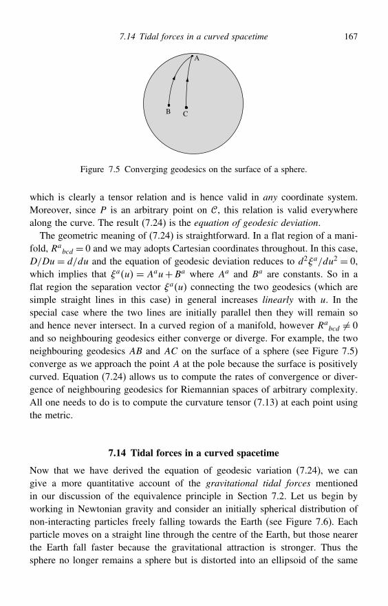
7.14 Tidal forces in a curved spacetime 167
A
B C
Figure 7.5 Converging geodesics on the surface of a sphere.
which is clearly a tensor relation and is hence valid in any coordinate system.Moreover, since P is an arbitrary point on , this relation is valid everywherealong the curve. The result (7.24) is the equation of geodesic deviation.
The geometric meaning of (7.24) is straightforward. In a flat region of a mani-fold, Ra
bcd = 0 and we may adopts Cartesian coordinates throughout. In this case,D/Du= d/du and the equation of geodesic deviation reduces to d2a/du2 = 0,which implies that au = Aau+Ba where Aa and Ba are constants. So in aflat region the separation vector au connecting the two geodesics (which aresimple straight lines in this case) in general increases linearly with u. In thespecial case where the two lines are initially parallel then they will remain soand hence never intersect. In a curved region of a manifold, however Ra
bcd = 0and so neighbouring geodesics either converge or diverge. For example, the twoneighbouring geodesics AB and AC on the surface of a sphere (see Figure 7.5)converge as we approach the point A at the pole because the surface is positivelycurved. Equation (7.24) allows us to compute the rates of convergence or diver-gence of neighbouring geodesics for Riemannian spaces of arbitrary complexity.All one needs to do is to compute the curvature tensor (7.13) at each point usingthe metric.
7.14 Tidal forces in a curved spacetime
Now that we have derived the equation of geodesic variation (7.24), we cangive a more quantitative account of the gravitational tidal forces mentionedin our discussion of the equivalence principle in Section 7.2. Let us begin byworking in Newtonian gravity and consider an initially spherical distribution ofnon-interacting particles freely falling towards the Earth (see Figure 7.6). Eachparticle moves on a straight line through the centre of the Earth, but those nearerthe Earth fall faster because the gravitational attraction is stronger. Thus thesphere no longer remains a sphere but is distorted into an ellipsoid of the same
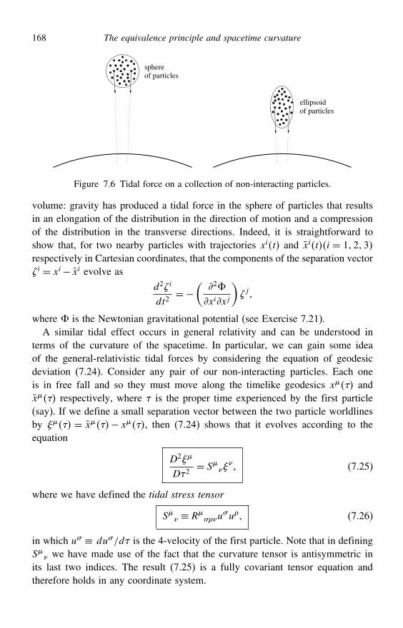
168 The equivalence principle and spacetime curvature
sphereof particles
ellipsoidof particles
Figure 7.6 Tidal force on a collection of non-interacting particles.
volume: gravity has produced a tidal force in the sphere of particles that resultsin an elongation of the distribution in the direction of motion and a compressionof the distribution in the transverse directions. Indeed, it is straightforward toshow that, for two nearby particles with trajectories xit and xiti = 123respectively in Cartesian coordinates, that the components of the separation vectori = xi− xi evolve as
d2i
dt2=−
(2%
xixj
)j
where % is the Newtonian gravitational potential (see Exercise 7.21).A similar tidal effect occurs in general relativity and can be understood in
terms of the curvature of the spacetime. In particular, we can gain some ideaof the general-relativistic tidal forces by considering the equation of geodesicdeviation (7.24). Consider any pair of our non-interacting particles. Each oneis in free fall and so they must move along the timelike geodesics x andx respectively, where is the proper time experienced by the first particle(say). If we define a small separation vector between the two particle worldlinesby = x− x, then (7.24) shows that it evolves according to theequation
D2
D2= S
(7.25)
where we have defined the tidal stress tensor
S ≡ R#u
#u (7.26)
in which u# ≡ du#/d is the 4-velocity of the first particle. Note that in definingS we have made use of the fact that the curvature tensor is antisymmetric inits last two indices. The result (7.25) is a fully covariant tensor equation andtherefore holds in any coordinate system.
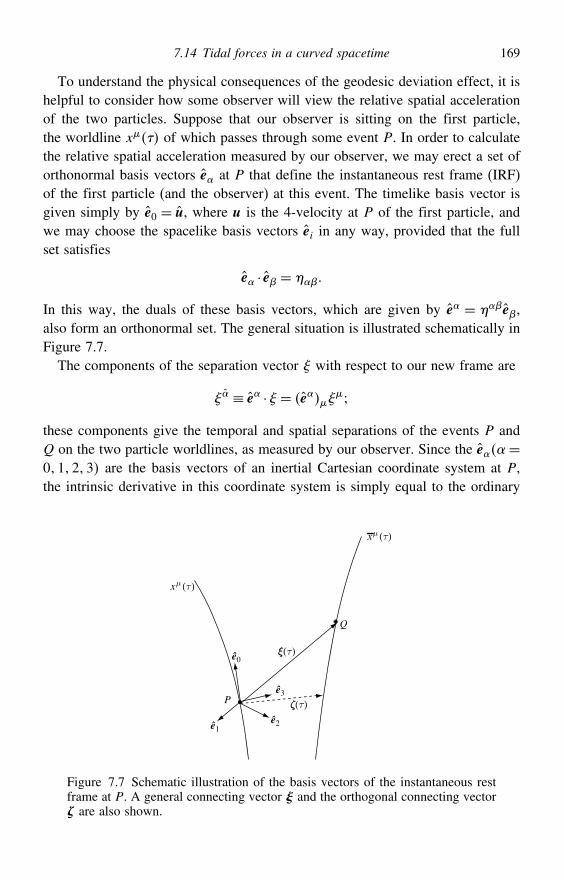
7.14 Tidal forces in a curved spacetime 169
To understand the physical consequences of the geodesic deviation effect, it ishelpful to consider how some observer will view the relative spatial accelerationof the two particles. Suppose that our observer is sitting on the first particle,the worldline x of which passes through some event P. In order to calculatethe relative spatial acceleration measured by our observer, we may erect a set oforthonormal basis vectors e at P that define the instantaneous rest frame (IRF)of the first particle (and the observer) at this event. The timelike basis vector isgiven simply by e0 = u, where u is the 4-velocity at P of the first particle, andwe may choose the spacelike basis vectors ei in any way, provided that the fullset satisfies
e · e =
In this way, the duals of these basis vectors, which are given by e = e,also form an orthonormal set. The general situation is illustrated schematically inFigure 7.7.
The components of the separation vector with respect to our new frame are
≡ e · = e
these components give the temporal and spatial separations of the events P andQ on the two particle worldlines, as measured by our observer. Since the e=0123 are the basis vectors of an inertial Cartesian coordinate system at P,the intrinsic derivative in this coordinate system is simply equal to the ordinary
ê0
ê1
ê3
ê2
ξ(τ)
xµ (τ)
ζ(τ)P
Q
xµ (τ)
Figure 7.7 Schematic illustration of the basis vectors of the instantaneous restframe at P. A general connecting vector and the orthogonal connecting vector are also shown.
170 The equivalence principle and spacetime curvature
derivative. Moreover, with respect to the IRF, the 4-velocity of the first particleis simply u= c 0. Thus from (7.25) we have
d2
d2= c2R
00 (7.27)
where the components of the curvature tensor in the Cartesian inertial frame at Pmay be written as
R ≡ R
#ee
#ee
(7.28)
Equation (7.27) in fact holds for any orthonormal freely falling frame e.Clearly, the general separation vector is inappropriate for our discussion of
the evolution of the spatial separation seen by our observer at P, since typically will have some temporal component in the observer’s frame. Thus, we mustwork instead with the orthogonal connecting vector shown in Figure 7.7,which has a zero component in the e0-direction, i.e.
0 = 0. Since (7.27) is validfor any small connecting vector it must also hold for the orthogonal connectingvector , but we must remember that 0= 0 for all .A useful alternative interpretation of (7.25) or (7.27) is that it gives the force
per unit mass required to keep two particles moving along parallel curves; thisforce must be supplied by some mechanical means. For example, the worldlineof the centre of mass of a rigid body in free fall is a timelike geodesic, but thisis not true of the other parts of the object, which are constrained to move alongcurves parallel to the centre of mass rather than along neighbouring geodesics.The necessary forces must be supplied by internal stresses in the object. Thephysical magnitude of the stresses is most easily found by solving the eigenvalueproblem
Sv = v (7.29)
where S is given by (7.26). One of the eigenvalues is always zero (for v= u),
and the remaining three eigenvalues give the principal stresses in the object.
Appendix 7A: The surface of a sphere
The metric5 of the surface of a sphere in spherical polar coordinates is
ds2 = a2 d2+a2 sin2 d2
5 Note that this term is often applied, as here, to the line element itself.
Appendix 7A: The surface of a sphere 171
To get used to handling problems involving curved spaces you should calculatethe components of the affine connection, starting from this metric. The definitionof the affine connection is
abc = 1
2gadbgdc+ cgbd− dgbc
as given in (3.21), and in two dimensions there are six independent connectioncoefficients,
111 1
12 122 2
11 212 2
22
These coefficients are given by (exercise):
111 = 1
2g111g11+ 1g11− 1g11= 0
112 = 1
2g112g11+ 2g21− 1g12= 0
122 = 1
2g112g21+ 2g21− 1g22=− 1
2g111g22
211 = 1
2g222g12+ 2g12− 2g11= 0
212 = 1
2g221g22+ 2g12− 2g11= 1
2g221g22
222 = 1
2g222g22+ 2g22− 2g22= 0
So, the only two non-zero coefficients are
122 = −
12a2
2a2 sin cos =− sin cos
212 =
1
2a2 sin2 2a2 sin cos = cos
sin
The curvature tensor is
Rabcd = 12dagbc− dbgac+ cbgad− cagbd−gef
eac
fbd− e
ad fbc
and in two dimensions the symmetry properties of this tensor mean that there isonly one independent component. We can take this to be R1212, so fortunately weonly have to calculate this single component:
R1212 = 1221g21− 22g11+ 12g12− 21g22−gef
e11
f22− e
12 f21
= − 12
21g22−g11
111
122− 1
12 112−g22
211
222− 2
21 221
= a2 sin2
Thus the Gaussian curvature K of a spherical surface is given by
K = R1212
g= a2 sin2
a4 sin2 = 1
a2
172 The equivalence principle and spacetime curvature
Instead of a spherical surface, we could instead consider the surface of acylinder of radius a. The metric of the surface in cylindrical polar coordinates is
ds2 = a2 d2+dz2
and it is obvious that this two-dimensional space is spatially flat because we cantransform the metric into the form
ds2 = dx2+dz2
by the coordinate transformation x = a. It therefore follows that the curvatureof a cylindrical surface vanishes.
Exercises
7.1 From Poisson’s equation 2% = 4G show that the gravitational potential outsidea spherical object of mass M at a radial distance r from its centre is given by%r=−GM/r. What is the form of %r inside a uniform spherical body?
7.2 A charged object held stationary in a laboratory on the surface of the Earth does notemit electromagnetic radiation. If the object is then dropped so that it is in free fall, itwill begin to radiate. Reconcile these observations with the principle of equivalence.Hint: Consider the spatial extent of the electric field of the charge.
7.3 If X is a local Cartesian coordinate system at some event P, show that so too is thecoordinate system X′ =$
X, where $
defines a Lorentz transformation.7.4 If two vectors v and w are Fermi–Walker-transported along some observer’s world-
line, show that their scalar product v ·w is preserved at all points along the line.7.5 Photons of frequency E are emitted from the surface of the Sun and observed by an
astronaut with fixed spatial coordinates at a large distance away. Obtain an expressionfor the frequency O of the photons as measured by the astronaut. Hence estimatethe observed redshift of the photon.
7.6 An experimenter A drops a pebble of rest mass m in a uniform gravitational field g.At a distance h below A, experimenter B converts the pebble (with no energy loss)into a photon of frequency B. The photon passes by A, who observes it to havefrequency A. Use simple physical arguments to show that to a first approximation
BA= 1+ gh
c2
Use this result to argue that for two stationary observers A and B in a weak gravi-tational field with potential %, the ratio of the rates at which their laboratory clocksrun is 1+%/c2, where % is the potential difference between A and B.
7.7 A satellite is in circular polar orbit of radius r around the Earth (radius R, mass M).A standard clock C on the satellite is compared with an identical clock C0 at the
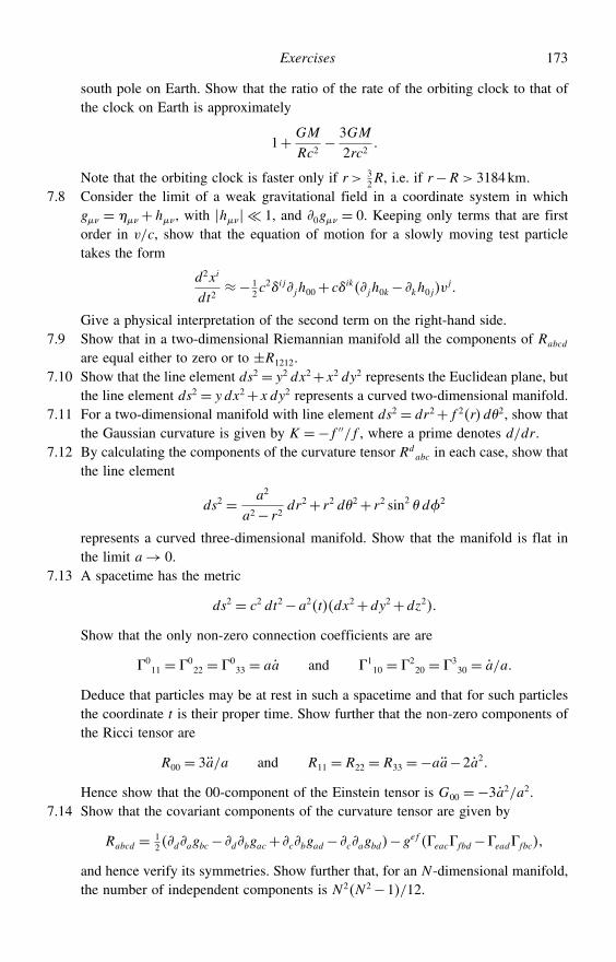
Exercises 173
south pole on Earth. Show that the ratio of the rate of the orbiting clock to that ofthe clock on Earth is approximately
1+ GM
Rc2− 3GM
2rc2
Note that the orbiting clock is faster only if r > 32R, i.e. if r−R > 3184km.
7.8 Consider the limit of a weak gravitational field in a coordinate system in whichg = +h, with h 1, and 0g = 0. Keeping only terms that are firstorder in v/c, show that the equation of motion for a slowly moving test particletakes the form
d2xi
dt2≈− 1
2c2ijjh00+ cikjh0k− kh0jv
j
Give a physical interpretation of the second term on the right-hand side.7.9 Show that in a two-dimensional Riemannian manifold all the components of Rabcd
are equal either to zero or to ±R1212.7.10 Show that the line element ds2 = y2 dx2+x2 dy2 represents the Euclidean plane, but
the line element ds2 = y dx2+xdy2 represents a curved two-dimensional manifold.7.11 For a two-dimensional manifold with line element ds2 = dr2+f 2rd2, show that
the Gaussian curvature is given by K =−f ′′/f , where a prime denotes d/dr.7.12 By calculating the components of the curvature tensor Rd
abc in each case, show thatthe line element
ds2 = a2
a2− r2dr2+ r2 d2+ r2 sin2 d2
represents a curved three-dimensional manifold. Show that the manifold is flat inthe limit a→ 0.
7.13 A spacetime has the metric
ds2 = c2 dt2−a2tdx2+dy2+dz2
Show that the only non-zero connection coefficients are are
011 = 0
22 = 033 = aa and 1
10 = 220 = 3
30 = a/a
Deduce that particles may be at rest in such a spacetime and that for such particlesthe coordinate t is their proper time. Show further that the non-zero components ofthe Ricci tensor are
R00 = 3a/a and R11 = R22 = R33 =−aa−2a2
Hence show that the 00-component of the Einstein tensor is G00 =−3a2/a2.7.14 Show that the covariant components of the curvature tensor are given by
Rabcd = 12 dagbc− dbgac+ cbgad− cagbd−gef eac fbd− ead fbc
and hence verify its symmetries. Show further that, for an N -dimensional manifold,the number of independent components is N 2N 2−1/12.
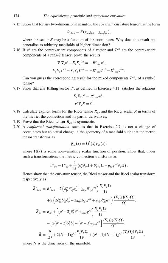
174 The equivalence principle and spacetime curvature
7.15 Show that for any two-dimensional manifold the covariant curvature tensor has the form
Rabcd = Kgacgbd−gadgbc
where the scalar K may be a function of the coordinates. Why does this result notgeneralise to arbitrary manifolds of higher dimension?
7.16 If va are the contravariant components of a vector and Tab are the contravariantcomponents of a rank-2 tensor, prove the results
cbva−bcv
a = −Radbcv
d
dcTab−cdT
ab = −RaecdT
eb−RbecdT
ae
Can you guess the corresponding result for the mixed components Tabc of a rank-3
tensor?7.17 Show that any Killing vector va, as defined in Exercise 4.11, satisfies the relations
cbva = Ra
bcdvd
vaaR = 0
7.18 Calculate explicit forms for the Ricci tensor Rab and the Ricci scalar R in terms ofthe metric, the connection and its partial derivatives.
7.19 Prove that the Ricci tensor Rab is symmetric.7.20 A conformal transformation, such as that in Exercise 2.7, is not a change of
coordinates but an actual change in the geometry of a manifold such that the metrictensor transforms as
gabx=2xgabx
where x is some non-vanishing scalar function of position. Show that, undersuch a transformation, the metric connection transforms as
abc = a
bc+1
(acb+abc−gbcg
add)
Hence show that the curvature tensor, the Ricci tensor and the Ricci scalar transformrespectively as
Rabcd = Ra
bcd−2(a c
ed
fb −gb c
edg
af) ef
+2(2a c
ed
fb −2gb c
edg
af +gb cadg
ef) ef
2
Rbc = Rbc+[N −2fb
ec+gbcg
ef] ef
−[2N −2fb
ec− N −3gbcg
ef] ef
2
R = R
2+2N −1gef
ef
3+ N −1N −4gef
ef
4
where N is the dimension of the manifold.
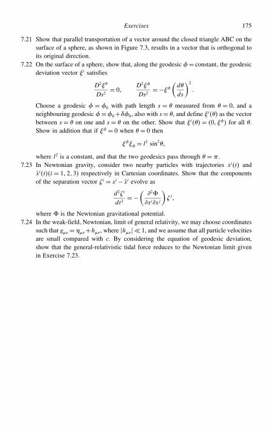
Exercises 175
7.21 Show that parallel transportation of a vector around the closed triangle ABC on thesurface of a sphere, as shown in Figure 7.3, results in a vector that is orthogonal toits original direction.
7.22 On the surface of a sphere, show that, along the geodesic = constant, the geodesicdeviation vector i satisfies
D2
Ds2= 0
D2
Ds2=−
(d
ds
)2
Choose a geodesic = 0 with path length s = measured from = 0, and aneighbouring geodesic =0+0, also with s= , and define i as the vectorbetween s = on one and s = on the other. Show that i= 0 for all .Show in addition that if = 0 when = 0 then
= l2 sin2
where l2 is a constant, and that the two geodesics pass through = .7.23 In Newtonian gravity, consider two nearby particles with trajectories xit and
xiti = 123 respectively in Cartesian coordinates. Show that the componentsof the separation vector i = xi− xi evolve as
d2i
dt2=−
(2%
xixj
)j
where % is the Newtonian gravitational potential.7.24 In the weak-field, Newtonian, limit of general relativity, we may choose coordinates
such that g =+h, where h 1, and we assume that all particle velocitiesare small compared with c. By considering the equation of geodesic deviation,show that the general-relativistic tidal force reduces to the Newtonian limit givenin Exercise 7.23.
8
The gravitational field equations
Let us now follow Einstein’s suggestion that gravity is a manifestation of space-time curvature induced by the presence of matter. We must therefore obtain a setof equations that describe quantitatively how the curvature of spacetime at anyevent is related to the matter distribution at that event. These will be the gravi-tational field equations, or Einstein equations, in the same way that the Maxwellequations are the field equations of electromagnetism.
Maxwell’s equations relate the electromagnetic field F at any event to itssource, the 4-current density j at that event. Similarly, Einstein’s equations relatespacetime curvature to its source, the energy–momentum of matter. As we shallsee, the analogy goes further. In any given coordinate system, Maxwell’s equa-tions are second-order partial differential equations for the components F ofthe electromagnetic field tensor (or equivalently for the components A of theelectromagnetic potential). We shall find that Einstein’s equations are also a set ofsecond-order partial differential equations, but instead for the metric coefficientsg of spacetime.
8.1 The energy–momentum tensor
To construct the gravitational field equations, we must first find a properly rela-tivistic (or covariant) way of expressing the source term. In other words, we mustidentify a tensor that describes the matter distribution at each event in spacetime.
We will use our discussion of the 4-current density in Chapter 6 as a guide. Thus,let us consider some general time-dependent distribution of (electrically neutral)non-interacting particles, each of rest mass m0. This is commonly called dust inthe literature. At each event P in spacetime we can characterise the distributioncompletely by giving the matter density and 3-velocity u as measured in someinertial frame. For simplicity, let us consider the fluid in its instantaneous restframe S at P, in which u = 0. In this frame, the (proper) density is given by
176
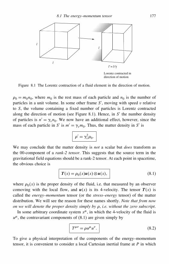
8.1 The energy–momentum tensor 177
l
Lorentz contracted indirection of motion
l'= l /γ
l
l
Figure 8.1 The Lorentz contraction of a fluid element in the direction of motion.
0 = m0n0, where m0 is the rest mass of each particle and n0 is the number ofparticles in a unit volume. In some other frame S′, moving with speed v relativeto S, the volume containing a fixed number of particles is Lorentz contractedalong the direction of motion (see Figure 8.1). Hence, in S′ the number densityof particles is n′ = vn0. We now have an additional effect, however, since themass of each particle in S′ is m′ = vm0. Thus, the matter density in S′ is
′ = 2v0
We may conclude that the matter density is not a scalar but does transform asthe 00-component of a rank-2 tensor. This suggests that the source term in thegravitational field equations should be a rank-2 tensor. At each point in spacetime,the obvious choice is
Tx= 0xux⊗ux (8.1)
where 0x is the proper density of the fluid, i.e. that measured by an observercomoving with the local flow, and ux is its 4-velocity. The tensor Tx iscalled the energy–momentum tensor (or the stress–energy tensor) of the matterdistribution. We will see the reason for these names shortly. Note that from nowon we will denote the proper density simply by , i.e. without the zero subscript.
In some arbitrary coordinate system x, in which the 4-velocity of the fluid isu, the contravariant components of (8.1) are given simply by
T = uu (8.2)
To give a physical interpretation of the components of the energy–momentumtensor, it is convenient to consider a local Cartesian inertial frame at P in which
178 The gravitational field equations
the set of components of the 4-velocity of the fluid is u = uc u. In thisframe, writing out the components in full we have
T 00 = u0u0 = 2uc
2
T 0i = T i0 = u0ui = 2ucu
i
T ij = uiuj = 2uu
iuj
Thus the physical meanings of these components in this frame are as follows:
T 00 is the energy density of the particles;T 0i is the energy flux× c−1 in the i-direction;T i0 is the momentum density× c in the i-direction;T ij is the rate of flow of the i-component of momentum per unit area in the
j-direction.
It is because of these identifications that the tensor T is known as the energy–momentum or stress–energy tensor.
8.2 The energy–momentum tensor of a perfect fluid
To generalise our discussion to real fluids, we have to take account of the facts that(i) besides the bulk motion of the fluid, each particle has some random (thermal)velocity and (ii) there may be various forces between the particles that contributepotential energies to the total. The physical meanings of the components of theenergy–momentum tensor T give us an insight into how to generalise its form toinclude these properties of real fluids.
Let us consider T at some event P and work in a local Cartesian inertial frameS that is the IRF of the fluid at P. For dust, the only non-zero component is T 00.However, let us consider the components of T in the IRF for a real fluid.
• T 00 is the total energy density, including any potential energy contributions from forcesbetween the particles and kinetic energy from their random thermal motions.
• T 0i: although there is no bulk motion, energy might be transmitted by heat conduction,so this is basically a heat conduction term in the IRF.
• T i0: again, although the particles have no bulk motion, if heat is being conducted thenthe energy will carry momentum.
• T ij: the random thermal motions of the particles will give rise to momentum flow,so that T ii is the isotropic pressure in the i-direction and the T ij (with i = j) are theviscous stresses in the fluid.
These identifications are valid for a general fluid. A perfect fluid is defined asone for which there are no forces between the particles, and no heat conduction
8.3 Conservation of energy and momentum for a perfect fluid 179
or viscosity in the IRF. Thus, in the IRF the components of T for a perfect fluidare given by
T=
⎛⎜⎜⎜⎝c2 0 0 00 p 0 00 0 p 00 0 0 p
⎞⎟⎟⎟⎠ (8.3)
It is not hard to show that
T = +p/c2uu−p (8.4)
However, because of the way in which we have written this equation, it mustbe valid in any local Cartesian inertial frame at P. Moreover, we can obtain anexpression that is valid in an arbitrary coordinate system simply by replacing with the metric functions g in the arbitrary system. Thus, we arrive at afully covariant expression for the components of the energy–momentum tensor ofa perfect fluid:
T = +p/c2uu−pg (8.5)
We see that T is symmetric and is made up from the two scalar fields and p
and the vector field u that characterise the perfect fluid. We also see that in thelimit p→ 0 a perfect fluid becomes dust.
Finally, we note that it is possible to give more complicated expressions repre-senting the energy–momentum tensors for imperfect fluids, for charged fluids andeven for the electromagnetic field. These tensors are all symmetric.
8.3 Conservation of energy and momentum for a perfect fluid
Let us investigate how to express energy and momentum conservation in a localCartesian inertial frame S at some event P that is represented by the local inertialcoordinates x. In these coordinates, the energy–momentum tensor takes theform (8.4).
By analogy with the equation j = 0 for the conservation of charge, which
we derived in Chapter 6, the conservation of energy and momentum is representedby the equation
T = 0 (8.6)
Rather than arriving at this result from first principles, which would take us intoa lengthy discussion of relativistic fluid mechanics, let us instead reverse the
180 The gravitational field equations
process and justify our assertion by arguing that it produces the correct equationsof motion and continuity for a fluid in the Newtonian limit.
Substituting the form (8.4) into (8.6) gives
+p/c2uu+ +p/c2 uu+uu
− p = 0 (8.7)
Now, the 4-velocity satisfies the normalisation condition uu = c2 and differenta-tion of this gives
uu+uu= 2u
u = 0
Thus, contracting (8.7) with u, dividing through by c2 and collecting terms gives
u+ p/c2u
= 0 (8.8)
Equation (8.7) therefore simplifies to
+p/c2uu = −uu/c2p (8.9)
Equations (8.8) and (8.9) are, in fact, respectively the relativistic equation ofcontinuity and the relativistic equation of motion for a perfect fluid in local inertialcoordinates at some event P.1 We will now show that for slowly moving fluidsand small pressures they reduce to the classical equations of Newtonian theory.
By a slowly moving fluid, we mean one for which we may neglect u/c and sotake u ≈ 1 and u≈ c u; note that the difference between the proper densityand the density disappears in this limit. By small pressures we mean that p/c2 isnegligible compared with . In these limits, equation (8.8) then reduces to
u= 0
or, in 3-vector notation,
t+ · u= 0
which is the classical equation of continuity for a fluid. In the limit of smallpressures, equation (8.9) reduces to
uu = −uu/c2p
Moreover, in our slowly-moving approximation, the zeroth components of theleft- and right-hand sides are both zero. Thus the spatial components i = 123satisfy
uiu =−jijp
1 As usual, these equations may be generalised to a form valid in arbitrary coordinates by replacing by
and replacing by g .
8.4 The Einstein equations 181
In 3-vector notation this reads
(
t+ u ·
)u=−p
which is Euler’s classical equation of motion for a perfect fluid. Hence we haveshown that the relativistic continuity equation (8.8) and the equation of motion(8.9) for a perfect fluid reduce to the appropriate Newtonian equations. If we wereto accept that a relativistic fluid were described by (8.8) and (8.9) then we couldreverse our overall argument and derive the result T
= 0.So far we have worked in local inertial coordinates in order to make contact
with the Newtonian theory. Nevertheless, we can trivially obtain the condition forenergy and momentum conservation in arbitrary coordinates by replacing by in (8.6), which then gives
T = 0 (8.10)
This important equation is worthy of further comment. In our discussion sofar, we have not been explicit about whether our spacetime is Minkowskian orcurved. Although the form (8.10) is valid (in arbitrary coordinates) in both cases,its interpretation differs in the two cases. If we neglect gravity and assume aMinkowski spacetime, the relation (8.10) does indeed represent the conservationof energy and momentum. In the presence of a gravitational field (and hencea curved spacetime), however, the energy and momentum of the matter aloneis not conserved. In this case, (8.10) represents the equation of motion of thematter under the influence of the gravitational field; this is discussed further inSection 8.8. As we will see below, the condition (8.10) places a tight restrictionon the possible forms that the gravitational field equations may take.
8.4 The Einstein equations
We are now in a position to deduce the form of the gravitational field equationsproposed by Einstein. Let us begin by recalling some of our previous results.
• The field equation of Newtonian gravity is
2% = 4G
• If gravity is a manifestation of spacetime curvature, we showed in Chapter 7, equa-tion (7.8), that for a weak gravitational field, in coordinates such that g = +h
(with h 1) and in which the metric is static, then
g00 =(1+ 2%
c2
) (8.11)
182 The gravitational field equations
• The correct relativistic description of matter is provided by the energy–momentumtensor and, for a perfect fluid or dust, in the IRF we have
T00 = c2
Combining these observations suggests that, for a weak static gravitational fieldin the low-velocity limit,
2g00 =8Gc4
T00
Einstein’s fundamental intuition was that the curvature of spacetime at anyevent is related to the matter content at that event. The above considerations thussuggest that the gravitational field equations should be of the form
K = &T (8.12)
where K is a rank-2 tensor related to the curvature of spacetime and we haveset &= 8G/c4. Since the curvature of spacetime is expressed by the curvaturetensor R#, the tensorK must be constructed from R# and the metric tensorg. Moreover, K should have the following properties: (i) the Newtonian limitsuggests that K should contain terms no higher than linear in the second-orderderivatives of the metric tensor; and (ii) since T is symmetric then K shouldalso be symmetric. The curvature tensor R# is already linear in the secondderivatives of the metric, and so the most general form for K that satisfies (i)and (ii) is
K = aR+bRg+g (8.13)
where R is the Ricci tensor, R is the curvature scalar and ab are constants.Let us now consider the constants ab. First, if we require that every term
in K is linear in the second derivatives of g then we see immediately that= 0. We will relax this condition later, but for the moment we therefore have
K = aR+bRg
To find the constants a and b we recall that the energy–momentum tensor satisfiesT
= 0; thus, from (8.10), we also require
K = aR
+bRg= 0
However, in Section 7.11 we showed that
R− 1
2gR= 0
and so, remembering that g = 0, we obtain
K = 12a+bgR= 0
8.5 The Einstein equations in empty space 183
The quantity R will, in general, be non-zero throughout (a region of) spacetimeunless the latter is flat and hence there is no gravitational field. Thus we find thatb =−a/2, and so the gravitational field equations must take the form
aR− 12gR= &T
To fix the constant a, we must compare the weak-field limit of these equationswith Poisson’s equation in Newtonian gravity. The comparison is presented in thenext section, where we show that, for consistency with the Newtonian theory, werequire a=−1 and so
R− 12gR=−&T (8.14)
where & = 8G/c4. Equation (8.14) constitutes Einstein’s gravitational fieldequations, which form the mathematical basis of the theory of general relativity.We note that the left-hand side of (8.14) is simply the Einstein tensorG, definedin Chapter 7.
We can obtain an alternative form of Einstein’s equations by writing (8.14) interms of mixed components,
R − 1
2 R=−&T
and contracting by setting = . We thus find that R = &T , where T ≡ T .
Hence we can write Einstein’s equations (8.14) as
R =−&T− 12Tg (8.15)
In four-dimensional spacetime g has 10 independent components and so ingeneral relativity we have 10 independent field equations. We may compare thiswith Newtonian gravity, in which there is only one gravitational field equation.Furthermore, the Einstein field equations are non-linear in the g whereas Newto-nian gravity is linear in the field %. Einstein’s theory thus involves numerousnon-linear differential equations, and so it should come as no surprise that thetheory is complicated.
8.5 The Einstein equations in empty space
In general, T contains all forms of energy and momentum. Of course, thisincludes any matter present but if there is also electromagnetic radiation, forexample, then it too must be included in T (the resulting expression is somewhatcomplicated; see Exercise 8.3).
184 The gravitational field equations
A region of spacetime in which T = 0 is called empty, and such a region istherefore not only devoid of matter but also of radiative energy and momentum. Itcan be seen from (8.15) that the gravitational field equations for empty space are
R = 0 (8.16)
From this simple equation, we can immediately establish a profound result.Consider the number of field equations as a function of the number of space-time dimensions; then, for two, three and four dimensions, the numbers of fieldequations and independent components of R# are as shown in the table.
No. of spacetime dimensions 2 3 4No. of field equations 3 6 10No. of independent components of R# 1 6 20
Thus we see that in two or three dimensions the field equations in empty spaceguarantee that the full curvature tensor must vanish. In four dimensions, however,we have 10 field equations but 20 independent components of the curvaturetensor. It is therefore possible to satisfy the field equations in empty space witha non-vanishing curvature tensor. Remembering that a non-vanishing curvaturetensor represents a non-vanishing gravitational field, we conclude that it is onlyin four dimensions or more that gravitational fields can exist in empty space.
8.6 The weak-field limit of the Einstein equations
To determine the ‘weak-field’ limit of the Einstein equations our preliminarydiscussion in Section 8.4 suggests that we need only consider their 00-component.It is most convenient to use the form (8.15) of the equations, from which we have
R00 =−&(T00− 1
2Tg00) (8.17)
In the weak-field approximation, spacetime is only ‘slightly’ curved and sothere exist coordinates in which g = +h, with h 1, and the metricis stationary. Hence in this case g00 ≈ 1. Moreover, from the definition of thecurvature tensor we find that R00 is given by
R00 = 0 0−
00+
0 0−
00
In our coordinate system the # are small, so we can neglect the last two
terms to first order in h. Also using the fact that the metric is stationary in ourcoordinate system, we then have
R00 ≈−i i00
8.7 The cosmological-constant term 185
In our discussion of the Newtonian limit in Chapter 7, however; we found that i
00 ≈ 12
ijjh00 to first order in h, and so
R00 ≈− 12
ijjh00
Substituting our approximate expressions for g00 and R00 into (8.17), in the‘weak-field’ limit we thus have
12
ijjh00 ≈ &I00− 12T (8.18)
To proceed further we must assume a form for the matter producing the weakgravitational field and for simplicity we consider a perfect fluid. Most classicalmatter distributions have p/c2 and so we may in fact take the energy–momentum tensor to be that of dust, i.e.
T = uu
which gives T = c2. In addition, let us assume that the particles making up thefluid have speeds u in our coordinate system that are small compared with c. Wethus make the approximation u ≈ 1 and hence u0 ≈ c. Therefore equation (8.18)reduces to
12
ijijh00 ≈ 12&c
2
We may, however, write ijij = 2; furthermore, from (8.11) we have h00 =2%/c2, where % is the gravitational potential. Thus, remembering that & =8G/c4, we finally obtain
2% ≈ 4G
which is Poisson’s equation in Newtonian gravity. This identification verifies ourearlier assertion that a=−1 in the derivation of Einstein’s equations (8.14).
8.7 The cosmological-constant term
The standard Einstein gravitational field equations are
R− 12gR=−&T (8.19)
However, these equations are not unique. In fact, shortly after Einstein derivedthem he proposed a modification known as the cosmological term.
In deriving the field equations (8.14), we assumed that the tensor K thatmakes up the left-hand side of the field equations,
K = &T
186 The gravitational field equations
should contain only terms that are linear in the second-order derivatives of g.This led us to set = 0 in (8.13), i.e. to discard the term g in the tensor K.Let us now relax this assumption.
Recalling that T = 0 we still require K
= 0, but in Section 4.12 weshowed that
g = 0
Thus, we can add any constant multiple of g to the left-hand side of (8.19) andstill obtain a consistent set of field equations. It is usual to denote this multipleby $, so that the field equations become
R− 12gR+$g =−&T (8.20)
where $ is some new universal constant of nature known as the cosmologicalconstant. By writing this equation in terms of the mixed components and contract-ing, as we did with the standard field equations, we find that R = &T + 4$.Substituting this expression into (8.20), we obtain an alternative form of the fieldequations,
R =−&(T− 1
2Tg)+$g (8.21)
Following the procedure presented in Section 8.6, it is straightforward to showthat, in the weak-field limit, the field equation of ‘Newtonian’ gravity becomes
2% = 4G−$c2
For a spherical mass M , the gravitational field strength is easily found to be
g =−% =−GM
r2r+ c2$r
3r
Thus, in this case, we see that the cosmological constant term corresponds to agravitational repulsion whose strength increases linearly with r.
The reason for calling $ the cosmological constant is historical. Einstein firstintroduced this term because he was unable to construct static models of theuniverse from his standard field equations (8.19). What he found (and we willdiscuss this in detail in Chapter 15) was that the standard field equations predicteda universe that was either expanding or contracting. Einstein did this work in about1916, when people thought that our Milky Way Galaxy represented the wholeuniverse, which Einstein represented as a uniform distribution of ‘fixed stars’.By introducing $, Einstein constructed static models of the universe (which aswe will see are actually unstable). It was later realised, however, that the MilkyWay is just one of a great many galaxies. Moreover, in 1929 Edwin Hubble
8.7 The cosmological-constant term 187
discovered the expansion of the universe by measuring distances and redshifts tonearby external galaxies. The universe was proved to be expanding and the needfor a cosmological constant disappeared. Einstein is reputed to have said that theintroduction of the cosmological constant was his ‘biggest blunder’.
Nowadays we have a rather different view of the cosmological constant. Recallthat the energy–momentum tensor of a perfect fluid is
T = +p/c2uu−pg
Imagine some type of ‘substance’ with a strange equation of state p=−c2. Thisis unlike any kind of substance that you have ever encountered because it has anegative pressure! The energy–momentum tensor for this substance would be
T =−pg = c2g
There are two points to note about this equation. First, the energy–momentumtensor of this strange substance depends only on the metric tensor – it is thereforea property of the vacuum itself and we can call the energy density of thevacuum. Second, the form of T is the same as the cosmological-constant termin (8.20). We can therefore view the cosmological constant as a universal constantthat fixes the energy density of the vacuum,
vacc2 = $c4
8G (8.22)
Denoting the energy–momentum tensor of the vacuum by T vac = vacc
2g, wecan thus write the modified gravitational field equations (8.20) as
R− 12gR=−&
(T+T vac
)
where T is the energy–momentum tensor of any matter or radiation present.How can we calculate the energy density of the vacuum? This is one of the
major unsolved problems in physics. The simplest calculation involves summingthe quantum mechanical zero-point energies of all the fields known in Nature.This gives an answer about 120 orders of magnitude higher than the upper limitson $ set by cosmological observations. This is probably the worst theoreticalprediction in the history of physics! Nobody knows how to make sense of thisresult. Some physical mechanism must exist that makes the cosmological constantvery small.
Some physicists have thought that A mechanism must exist that makes$ exactlyequal to zero. But in the last few years there has been increasing evidence thatthe cosmological constant is small but non-zero. The strongest evidence comes
188 The gravitational field equations
from observations of distant Type Ia supernovae that indicate that the expansion ofthe universe is actually accelerating rather than decelerating. Normally, one wouldhave thought that the gravity of matter in the universe would cause the expansionto slow down (perhaps even eventually halting the expansion and causing theuniverse to collapse). But if the cosmological constant is non-zero, the negativepressure of the vacuum can cause the universe to accelerate.
Whether these supernova observations are right or not is an area of activeresearch, and the theoretical problem of explaining the value of the cosmologicalconstant is one of the great challenges of theoretical physics. It is most likelythat we require a fully developed theory of quantum gravity (perhaps superstringtheory) before we can understand $.
8.8 Geodesic motion from the Einstein equations
The Einstein equations give a quantitative description of how the energy–momentum distribution of matter (or other fields) at any event determines thespacetime curvature at that event. We also know that, under the influence ofgravity alone, matter moves along geodesics in the curved spacetime. We nowshow that it is, in fact, unnecessary to make the separate postulate of geodesicmotion, since it follows directly from the Einstein equations themselves.
The field equations were derived partly from the requirement that the covariantdivergence of the energy–momentum tensor vanishes,
T = 0 (8.23)
As noted in Section 8.3, this relation represents the equation of motion for matterin the curved spacetime, and in this section we explore this interpretation in moredetail. For later convenience, we may also write (8.23) as
T = T
+ #T
#+ #T
#
= 1√−g √−gT+
#T# (8.24)
where in the last line we have used the expression (3.26) for the contractedconnection coefficient
#, and we note that g = −g for a spacetime metricwith signature −2.
Let us first consider directly the specific case of a single test particle of restmass m. By analogy with (8.2), the energy–momentum tensor of the particle as afunction of position x may be written as
Tx= m√−g∫ dz
d
dz
d4x− zd (8.25)
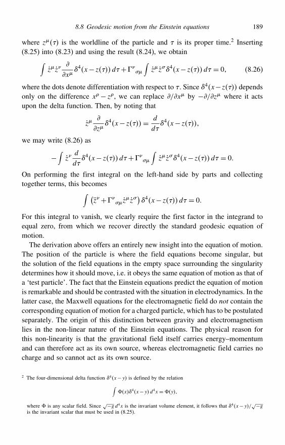
8.8 Geodesic motion from the Einstein equations 189
where z is the worldline of the particle and is its proper time.2 Inserting(8.25) into (8.23) and using the result (8.24), we obtain∫
zz
x4x− zd+
#
∫zz#4x− zd = 0 (8.26)
where the dots denote differentiation with respect to . Since 4x−z dependsonly on the difference x− z, we can replace /x by −/z where it actsupon the delta function. Then, by noting that
z
z4x− z= d
d4x− z
we may write (8.26) as
−∫z
d
d4x− zd+
#
∫zz#4x− zd = 0
On performing the first integral on the left-hand side by parts and collectingtogether terms, this becomes∫ (
z+ #z
z#)4x− zd = 0
For this integral to vanish, we clearly require the first factor in the integrand toequal zero, from which we recover directly the standard geodesic equation ofmotion.
The derivation above offers an entirely new insight into the equation of motion.The position of the particle is where the field equations become singular, butthe solution of the field equations in the empty space surrounding the singularitydetermines how it should move, i.e. it obeys the same equation of motion as that ofa ‘test particle’. The fact that the Einstein equations predict the equation of motionis remarkable and should be contrasted with the situation in electrodynamics. In thelatter case, the Maxwell equations for the electromagnetic field do not contain thecorresponding equation of motion for a charged particle, which has to be postulatedseparately. The origin of this distinction between gravity and electromagnetismlies in the non-linear nature of the Einstein equations. The physical reason forthis non-linearity is that the gravitational field itself carries energy–momentumand can therefore act as its own source, whereas electromagnetic field carries nocharge and so cannot act as its own source.
2 The four-dimensional delta function 4x−y is defined by the relation∫%x4x−yd4x =%y
where % is any scalar field. Since√−g d4x is the invariant volume element, it follows that 4x−y/
√−gis the invariant scalar that must be used in (8.25).
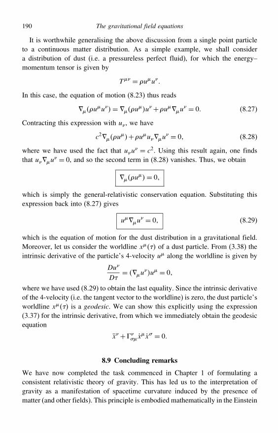
190 The gravitational field equations
It is worthwhile generalising the above discussion from a single point particleto a continuous matter distribution. As a simple example, we shall considera distribution of dust (i.e. a pressureless perfect fluid), for which the energy–momentum tensor is given by
T = uu
In this case, the equation of motion (8.23) thus reads
uu= u
u+uu = 0 (8.27)
Contracting this expression with u, we have
c2u+uuu
= 0 (8.28)
where we have used the fact that uu = c2. Using this result again, one finds
that uu = 0, and so the second term in (8.28) vanishes. Thus, we obtain
u= 0
which is simply the general-relativistic conservation equation. Substituting thisexpression back into (8.27) gives
uu = 0 (8.29)
which is the equation of motion for the dust distribution in a gravitational field.Moreover, let us consider the worldline x of a dust particle. From (3.38) theintrinsic derivative of the particle’s 4-velocity u along the worldline is given by
Du
D= u
u = 0
where we have used (8.29) to obtain the last equality. Since the intrinsic derivativeof the 4-velocity (i.e. the tangent vector to the worldline) is zero, the dust particle’sworldline x is a geodesic. We can show this explicitly using the expression(3.37) for the intrinsic derivative, from which we immediately obtain the geodesicequation
x+ #x
x# = 0
8.9 Concluding remarks
We have now completed the task commenced in Chapter 1 of formulating aconsistent relativistic theory of gravity. This has led us to the interpretation ofgravity as a manifestation of spacetime curvature induced by the presence ofmatter (and other fields). This principle is embodied mathematically in the Einstein
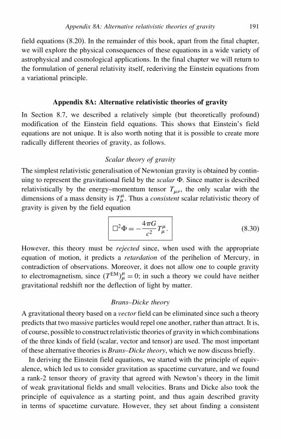
Appendix 8A: Alternative relativistic theories of gravity 191
field equations (8.20). In the remainder of this book, apart from the final chapter,we will explore the physical consequences of these equations in a wide variety ofastrophysical and cosmological applications. In the final chapter we will return tothe formulation of general relativity itself, rederiving the Einstein equations froma variational principle.
Appendix 8A: Alternative relativistic theories of gravity
In Section 8.7, we described a relatively simple (but theoretically profound)modification of the Einstein field equations. This shows that Einstein’s fieldequations are not unique. It is also worth noting that it is possible to create moreradically different theories of gravity, as follows.
Scalar theory of gravity
The simplest relativistic generalisation of Newtonian gravity is obtained by contin-uing to represent the gravitational field by the scalar %. Since matter is describedrelativistically by the energy–momentum tensor T, the only scalar with thedimensions of a mass density is T
. Thus a consistent scalar relativistic theory ofgravity is given by the field equation
2% =−4G
c2T (8.30)
However, this theory must be rejected since, when used with the appropriateequation of motion, it predicts a retardation of the perihelion of Mercury, incontradiction of observations. Moreover, it does not allow one to couple gravityto electromagnetism, since TEM
= 0; in such a theory we could have neither
gravitational redshift nor the deflection of light by matter.
Brans–Dicke theory
A gravitational theory based on a vector field can be eliminated since such a theorypredicts that two massive particles would repel one another, rather than attract. It is,of course, possible to construct relativistic theories of gravity inwhich combinationsof the three kinds of field (scalar, vector and tensor) are used. The most importantof these alternative theories is Brans–Dicke theory, which we now discuss briefly.
In deriving the Einstein field equations, we started with the principle of equiv-alence, which led us to consider gravitation as spacetime curvature, and we founda rank-2 tensor theory of gravity that agreed with Newton’s theory in the limitof weak gravitational fields and small velocities. Brans and Dicke also took theprinciple of equivalence as a starting point, and thus again described gravityin terms of spacetime curvature. However, they set about finding a consistent
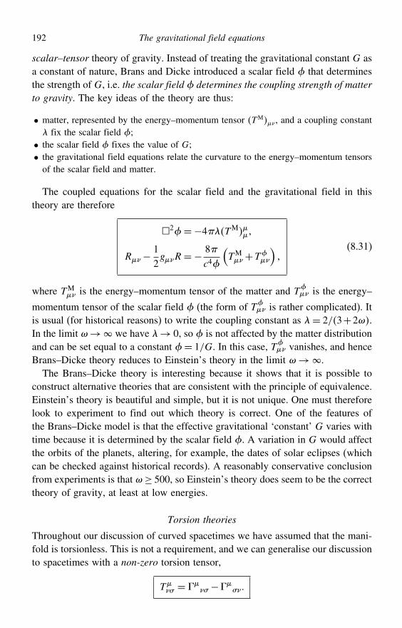
192 The gravitational field equations
scalar–tensor theory of gravity. Instead of treating the gravitational constant G asa constant of nature, Brans and Dicke introduced a scalar field that determinesthe strength of G, i.e. the scalar field determines the coupling strength of matterto gravity. The key ideas of the theory are thus:
• matter, represented by the energy–momentum tensor TM, and a coupling constant fix the scalar field ;
• the scalar field fixes the value of G;• the gravitational field equations relate the curvature to the energy–momentum tensorsof the scalar field and matter.
The coupled equations for the scalar field and the gravitational field in thistheory are therefore
2=−4TM
R−12gR=−
8c4
(TM+T
)
(8.31)
where TM is the energy–momentum tensor of the matter and T
is the energy–
momentum tensor of the scalar field (the form of T is rather complicated). It
is usual (for historical reasons) to write the coupling constant as = 2/3+2.In the limit → we have → 0, so is not affected by the matter distributionand can be set equal to a constant = 1/G. In this case, T
vanishes, and henceBrans–Dicke theory reduces to Einstein’s theory in the limit →.
The Brans–Dicke theory is interesting because it shows that it is possible toconstruct alternative theories that are consistent with the principle of equivalence.Einstein’s theory is beautiful and simple, but it is not unique. One must thereforelook to experiment to find out which theory is correct. One of the features ofthe Brans–Dicke model is that the effective gravitational ‘constant’ G varies withtime because it is determined by the scalar field . A variation in G would affectthe orbits of the planets, altering, for example, the dates of solar eclipses (whichcan be checked against historical records). A reasonably conservative conclusionfrom experiments is that ≥ 500, so Einstein’s theory does seem to be the correcttheory of gravity, at least at low energies.
Torsion theories
Throughout our discussion of curved spacetimes we have assumed that the mani-fold is torsionless. This is not a requirement, and we can generalise our discussionto spacetimes with a non-zero torsion tensor,
T# =
# − #
Exercises 193
Typically, torsion is generated by the (quantum-mechanical) spin of particles.Such theories are rather complicated mathematically, since we must make thedistinction between affine and metric connections and geodesics. Gravitationaltheories that include spacetime torsion are often described as Einstein–Cartantheories and have been extensively investigated. We will not discuss these theoriesany further, however.
Appendix 8B: Sign conventions
There is no accepted system of sign conventions in general relativity. Differentbooks use different sign conventions for the metric tensor, for the curvature tensorsand for the field equations. We can summarize these sign conventions in termsof three sign factors S1, S2 and S3. These are defined as follows:
= S1 −1+1+1+1 R
= S2(
−
+
# #−
# #
)
G = S38Gc4
T
R = S2 S3R
In this text we have used a convention that matches that of both R. d’Inverno,An Introduction to Einstein’s Relativity, Oxford University Press, 1992, andW. Rindler, Relativity: Special, General and Cosmological, Oxford UniversityPress, 2001, but this differs from the convention used by, for example, Misner,Thorne and Wheeler, Gravitation, Freeman (1973) or Weinberg, Gravitation andCosmology, Wiley, (1972). Here is a summary of the sign conventions used inthe various books:
Present text d’Inverno, Rindler MTW Weinberg S1 − − + + S2 + + + − S3 − − + −
Exercises
8.1 Show that the components of the energy–momentum tensor of a perfect fluid in itsinstantaneous rest frame can be written as in (8.3):
T = +p/c2uu−p
Can the components be written in any other covariant form?8.2 Show that, for any fluid,
uu = 0
194 The gravitational field equations
Hence show that a perfect fluid in a gravitational field must satisfy the equations
u+ p
c2u
= 0(+ p
c2
)uu
=(g− uu
c2
)p
Obtain the equation of motion for the worldline x of a particle in a perfect fluidwith pressure, and hence show that the particle is ‘pushed off’ geodesics by thepressure gradient.
8.3 The electromagnetic field in vacuo has an energy–momentum tensor Tem . By analogy
with the energy–momentum tensor for dust, we require that (i) Tem is symmetric;
(ii) Tem = 0; (iii) T
em must be quadratic in the dynamical variable F. Henceshow that
Tem = F
#F# − 1
4gF#F
#
where is a constant. By examining the component T 00em in local Cartesian inertial
coordinates, show that the constant =−1/0.8.4 Consider a cloud of charged dust particles. Show that the equation of motion of such
a fluid is
uu = #F
u
where is the proper matter density of the fluid, # is its proper charge density andu is the fluid 4-velocity. Define an energy–momentum tensor T
d = uu, where is the proper density of the fluid. Hence show that
Td = F
j
Tem = −F
j
where j = #u is the 4-current density. Thus write down the energy–momentumtensor for charged dust, T = T
d +T
em .8.5 The energy–momentum tensor of an electromagnetic field interacting with a source
satisfies Tem = −F#J# , where J# is the 4-current density of the source. Hence
show that the worldline of a particle of charge q in an electromagnetic field satisfies
z+ #z
z# = q
mF
# z#
and interpret this result physically.8.6 The weak energy condition (WEC) states that any energy–momentum tensor must
satisfy
Ttt ≥ 0
for all timelike vectors t. Show that for a perfect fluid the WEC implies that
≥ 0 and c2+p ≥ 0
Exercises 195
8.7 The strong energy condition (SEC) states that any energy–momentum tensor mustsatisfy
Ttt ≥ 1
2T t
#t#
for all timelike vectors t. Show that for a perfect fluid the SEC implies that
c2+p ≥ 0 and c2+3p ≥ 0
Does the SEC imply the WEC in Exercise 8.7? Show further that, from the Einsteinequations, the SEC implies that Rt
t ≥ 0, where R is the Ricci tensor.8.8 The equation-of-state parameter w is defined by w = p/c2. If one restricts
oneself to sources for which ≥ 0, show that both the weak and strong energyconditions in Exercises 8.6 and 8.7 imply that w ≥−1.
8.9 Write down the form of the energy–momentum tensor for a perfect fluid with4-velocity u with respect to some Cartesian inertial frame S. Show that for theenergy–momentum tensor to be invariant under a Lorentz transformation to anyother inertial frame one requires p = −c2. Compare this result with that for theenergy–momentum tensor of the vacuum.
8.10 Find the most general tensor which can be constructed from the curvature tensorand the metric tensor and which contains terms no higher than quadratic in thesecond-order derivatives of g. Hence write down the most general form of thegravitational field equations in such a theory.
8.11 In the Newtonian limit of weak gravitational fields, for a slowly moving perfect fluidwith pressure p c2 show that the 00-component of the Einstein field equationswith a non-zero cosmological constant $ reduces to
2% = 4G−$c2
where 2 = ijij and is the proper density of the fluid. Hence show that thecorresponding Newtonian gravitational potential of a spherically symmetric massM centred at the origin can be written as
% =−GM
r− $c2r2
6
where r2 = ijxixj . Give a physical interpretation of this result.8.12 In the scalar theory of gravity (8.30) show that, in any inertial frame, the gravitational
potential % produced by a perfect fluid at some event P satisfies
1c2
2%
t2− 2% =−4G
(− 3p
c2
)
where and p are the density and isotropic pressure as measured in the instantaneousrest frame of the fluid at P. Hence show that the theory reduces to Newtoniangravity in the non-relativistic limit. How might a cosmological constant be includedin the theory?
9
The Schwarzschild geometry
We now consider how to solve the Einstein field equations and so discover themetric functions g in any given physical situation. Clearly, the high degree ofnon-linearity in the field equations means that a general solution for an arbitrarymatter distribution is analytically intractable. The problem becomes easier if welook for special solutions, for example those representing spacetimes possessingsymmetries. The first exact solution to Einstein’s equations was found by KarlSchwarzschild in 1916.1 As we shall see, the Schwarzschild solution representsthe spacetime geometry outside a spherically symmetric matter distribution.
9.1 The general static isotropic metric
Schwarzschild sought the metric g representing the static spherically symmetricgravitational field in the empty space surrounding some massive spherical objectsuch as a star. Thus, a good starting point for us is to construct the most generalform of the metric for a static spatially isotropic spacetime.
A static spacetime is one for which some timelike coordinate x0 (say) with thefollowing properties: (i) all the metric components g are independent of x
0; and(ii) the line element ds2 is invariant under the transformation x0→−x0. Note that(i) does not necessarily imply (ii), as is made clear by the example of a rotatingstar: time reversal changes the sense of rotation, but the metric components areconstant in time. A spacetime that satisfies (i) but not (ii) is called stationary.
Thus, starting from the general expression for the line element
ds2 = g dx dx
we wish to find a set of coordinates x in which the g do not depend on thetimelike coordinate x0 and the line element ds2 is invariant under x0→−x0, i.e.1 Astonishingly, Schwarzschild derived the solution while in the trenches on the Eastern Front during the FirstWorld War but sadly he did not survive the conflict.
196
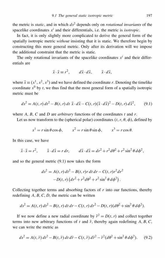
9.1 The general static isotropic metric 197
the metric is static, and in which ds2 depends only on rotational invariants of thespacelike coordinates xi and their differentials, i.e. the metric is isotropic.
In fact, it is only slightly more complicated to derive the general form of thespatially isotropic metric without insisting that it is static. We therefore begin byconstructing this more general metric. Only after its derivation will we imposethe additional constraint that the metric is static.
The only rotational invariants of the spacelike coordinates xi and their differ-entials are
x · x ≡ r2 dx ·dx x ·dx
where x≡ x1 x2 x3 and we have defined the coordinate r. Denoting the timelikecoordinate x0 by t, we thus find that the most general form of a spatially isotropicmetric must be
ds2 = At rdt2−Bt rdt x ·dx−Ct rx ·dx2−Dt rdx2 (9.1)
where A, B, C and D are arbitrary functions of the coordinates t and r.Let us now transform to the (spherical polar) coordinates t r , defined by
x1 = r sin cos x2 = r sin sin x3 = r cos
In this case, we have
x · x = r2 x ·dx = r dr dx ·dx = dr2+ r2d2+ r2 sin2 d2
and so the general metric (9.1) now takes the form
ds2 = At rdt2−Bt rr dt dr−Ct rr2dr2
−Dt r (dr2+ r2d2+ r2 sin2 d2) Collecting together terms and absorbing factors of r into our functions, therebyredefining ABCD, the metric can be written
ds2 = At rdt2−Bt rdt dr−Ct rdr2−Dt rd2+ sin2 d2
If we now define a new radial coordinate by r2 = Dt r and collect togetherterms into new arbitrary functions of t and r, thereby again redefining ABC,we can write the metric as
ds2 = At r dt2−Bt r dt dr−Ct r dr2− r2d2+ sin2 d2 (9.2)
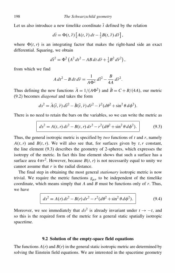
198 The Schwarzschild geometry
Let us also introduce a new timelike coordinate t defined by the relation
dt =%t r[At r dt− 1
2Bt r dr]
where %t r is an integrating factor that makes the right-hand side an exactdifferential. Squaring, we obtain
dt2 =%2 (A2 dt2−ABdt dr+ 14B
2 dr2)
from which we find
Adt2−Bdt dr = 1A%2
dt2− B
4Adr2
Thus defining the new functions A= 1/A%2 and B = C+B/4A, our metric(9.2) becomes diagonal and takes the form
ds2 = At r dt2− Bt r dr2− r2d2+ sin2 d2
There is no need to retain the bars on the variables, so we can write the metric as
ds2 = At rdt2−Bt rdr2− r2d2+ sin2 d2 (9.3)
Thus, the general isotropic metric is specified by two functions of t and r, namelyAt r and Bt r. We will also see that, for surfaces given by t r constant,the line element (9.3) describes the geometry of 2-spheres, which expresses theisotropy of the metric. In fact this line element shows that such a surface has asurface area 4r2. However, because Bt r is not necessarily equal to unity wecannot assume that r is the radial distance.
The final step in obtaining the most general stationary isotropic metric is nowtrivial. We require the metric functions g to be independent of the timelikecoordinate, which means simply that A and B must be functions only of r. Thus,we have
ds2 = Ardt2−Brdr2− r2d2+ sin2 d2 (9.4)
Moreover, we see immediately that ds2 is already invariant under t→−t, andso this is the required form of the metric for a general static spatially isotropicspacetime.
9.2 Solution of the empty-space field equations
The functionsAr and Br in the general static isotropic metric are determined bysolving the Einstein field equations. We are interested in the spacetime geometry
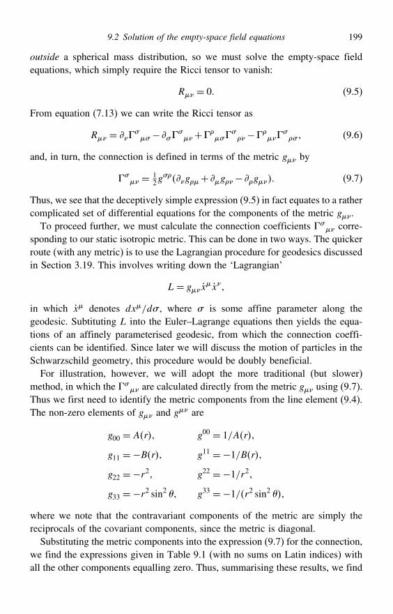
9.2 Solution of the empty-space field equations 199
outside a spherical mass distribution, so we must solve the empty-space fieldequations, which simply require the Ricci tensor to vanish:
R = 0 (9.5)
From equation (7.13) we can write the Ricci tensor as
R = ## − #
#+
# #−
## (9.6)
and, in turn, the connection is defined in terms of the metric g by
# = 1
2g#g+ g− g (9.7)
Thus, we see that the deceptively simple expression (9.5) in fact equates to a rathercomplicated set of differential equations for the components of the metric g.To proceed further, we must calculate the connection coefficients #
corre-sponding to our static isotropic metric. This can be done in two ways. The quickerroute (with any metric) is to use the Lagrangian procedure for geodesics discussedin Section 3.19. This involves writing down the ‘Lagrangian’
L= gxx
in which x denotes dx/d# , where # is some affine parameter along thegeodesic. Subtituting L into the Euler–Lagrange equations then yields the equa-tions of an affinely parameterised geodesic, from which the connection coeffi-cients can be identified. Since later we will discuss the motion of particles in theSchwarzschild geometry, this procedure would be doubly beneficial.
For illustration, however, we will adopt the more traditional (but slower)method, in which the #
are calculated directly from the metric g using (9.7).Thus we first need to identify the metric components from the line element (9.4).The non-zero elements of g and g are
g00 = Ar g00 = 1/Ar
g11 =−Br g11 =−1/Brg22 =−r2 g22 =−1/r2g33 =−r2 sin2 g33 =−1/r2 sin2
where we note that the contravariant components of the metric are simply thereciprocals of the covariant components, since the metric is diagonal.
Substituting the metric components into the expression (9.7) for the connection,we find the expressions given in Table 9.1 (with no sums on Latin indices) withall the other components equalling zero. Thus, summarising these results, we find
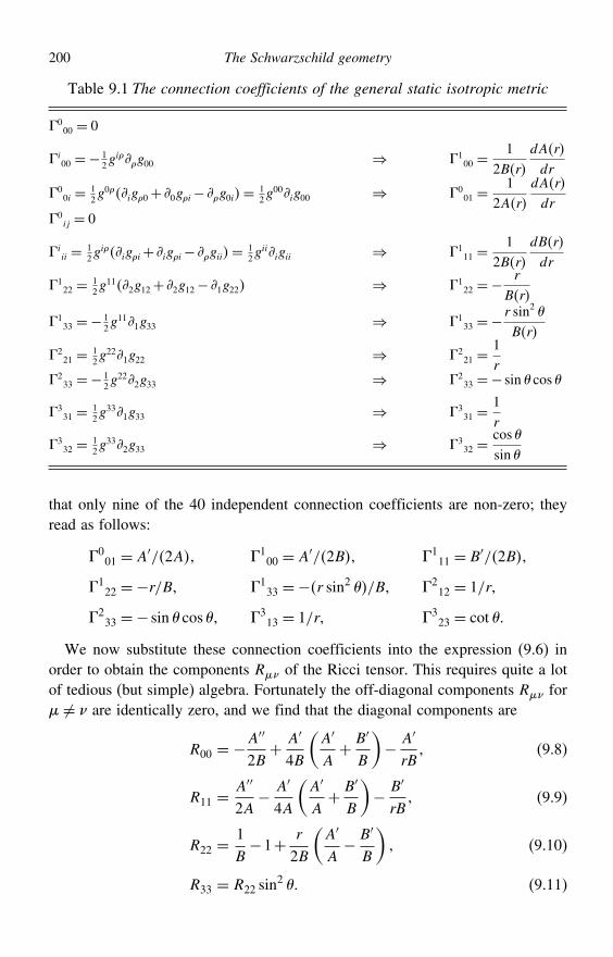
200 The Schwarzschild geometry
Table 9.1 The connection coefficients of the general static isotropic metric
000 = 0
i00 =− 1
2gig00 ⇒ 1
00 =1
2BrdAr
dr
00i = 1
2g0ig0+ 0gi− g0i= 1
2g00ig00 ⇒ 0
01 =1
2ArdAr
dr 0
ij = 0
iii = 1
2giigi+ igi− gii= 1
2giiigii ⇒ 1
11 =1
2BrdBr
dr
122 = 1
2g112g12+ 2g12− 1g22 ⇒ 1
22 =−r
Br
133 =− 1
2g111g33 ⇒ 1
33 =−r sin2 Br
221 = 1
2g221g22 ⇒ 2
21 =1r
233 =− 1
2g222g33 ⇒ 2
33 =− sin cos
331 = 1
2g331g33 ⇒ 3
31 =1r
332 = 1
2g332g33 ⇒ 3
32 =cossin
that only nine of the 40 independent connection coefficients are non-zero; theyread as follows:
001 = A′/2A 1
00 = A′/2B 111 = B′/2B
122 =−r/B 1
33 =−r sin2 /B 212 = 1/r
233 =− sin cos 3
13 = 1/r 323 = cot
We now substitute these connection coefficients into the expression (9.6) inorder to obtain the components R of the Ricci tensor. This requires quite a lotof tedious (but simple) algebra. Fortunately the off-diagonal components R for = are identically zero, and we find that the diagonal components are
R00 = −A′′
2B+ A′
4B
(A′
A+ B′
B
)− A′
rB (9.8)
R11 =A′′
2A− A′
4A
(A′
A+ B′
B
)− B′
rB (9.9)
R22 =1B−1+ r
2B
(A′
A− B′
B
) (9.10)
R33 = R22 sin2 (9.11)
9.2 Solution of the empty-space field equations 201
The empty-space field equations (9.5) are thus obtained by setting each of theexpressions (9.8–9.11) equal to zero. Of these four equations, only the first threeare useful, since the fourth merely repeats the information contained in the third.Adding B/A times (9.8) to (9.9) and rearranging gives
A′B+AB′ = 0
which implies that AB = constant. Let us denote this constant by . SubstitutingB = /A into (9.10) we obtain A+ rA′ = , which can be written as
drA
dr=
Integrating this equation gives rA = r + k, where k is another integrationconstant. Thus the functions Ar and Br are given by
Ar=
(1+ k
r
)and Br=
(1+ k
r
)−1
In solving for A and B we have used only the sum of equations (9.8) and (9.9),not the separate equations. It is, however, straightforward to check that, with theseforms for A and B, the equations (9.8–9.11) are satisfied separately.
It can be seen that the integration constant k must in some way represent themass of the object producing the gravitational field, as follows. We can identifyk (and ) by considering the weak-field limit, in which we require that
Ar
c2→ 1+ 2%
c2
where % is the Newtonian gravitational potential. Moreover, in the weak-fieldlimit r can be identified as the radial distance, to a very good approximation. Fora spherically symmetric mass M we thus have %=−GM/r, and so we concludethat k=−2GM/c2 and = c2. Therefore, the Schwarzschild metric for the emptyspacetime outside a spherical body of mass M is2
ds2 = c2(1− 2GM
c2r
)dt2−
(1− 2GM
c2r
)−1dr2− r2 d2− r2 sin2 d2
(9.12)
We will use this metric to investigate the physics in the vicinity of a sphericalobject of mass M , in particular the trajectories of freely falling massive particles
2 We note that the constant could have been identified earlier by making the additional assumption thatspacetime is asymptotically flat, i.e. that the line element (9.4) tends to the Minkowski line element in thelimit r→. Thus we require that, in this limit, Ar→ c2 and Br→ 1 and so AB = c2.
202 The Schwarzschild geometry
and photons. The Schwarzschild metric is valid down to the surface of the spheri-cal object, at which point the empty-space field equations no longer hold. Clearly,the metric functions are infinite at r = 2, which is known as the Schwarzschildradius. As we shall see, if the surface of the massive body contracts within thisradius then the object becomes a Schwarzschild black hole (see Chapter 11). Forthe remainder of this chapter, however, we will restrict our attention to the regionr > 2GM/c2. We will often use the shorthand ≡ GM/c2 when writing downthis metric.
9.3 Birkhoff’s theorem
If we do not demand that our original metric is static (or stationary) but only thatit is isotropic, then we would substitute the more general form (9.3),
ds2 = At rdt2−Bt rdr2− r2d2+ sin2 d2
into Einstein’s empty-space field equations R = 0 in order to determine thefunctions At r and Bt r. On repeating our earlier analysis, we would findsome additional non-zero connection coefficients and components of the Riccitensor. However, on solving this new set of equations, one discovers that theresulting metric must still be the Schwarzschild metric (9.12). Thus, we obtainBirkhoff’s theorem, which states that the spacetime geometry outside a generalspherically symmetric matter distribution is the Schwarzschild geometry.
This is an unexpected result because in Newtonian theory spherical symmetryhas nothing to do with time dependence. This highlights the special character ofthe empty-space Einstein equations and of the solutions they admit. In particular,Birkhoff’s theorem implies that if a spherically symmetric star undergoes strictlyradial pulsations then it cannot propagate any disturbance into the surroundingspace. Looking ahead to Chapter 18, this means that a radially pulsating starcannot emit gravitational waves.
One can show that the converse of Birkhoff’s theorem is not true, i.e. a matterdistribution that gives rise to the Schwarzschild geometry outside it need not bespherically symmetric. Indeed, some specific counter-examples are known.
9.4 Gravitational redshift for a fixed emitter and receiver
We begin our discussion of the physics in the vicinity of a spherical mass M byconsidering the phenomenon of gravitational redshift. In particular, we considerthe specific example of an emitter, at fixed spatial coordinates rE EE,which emits a photon that is received by an observer at fixed spatial coordinatesrR RR. If tE is the coordinate time of emission and tR the coordinate time
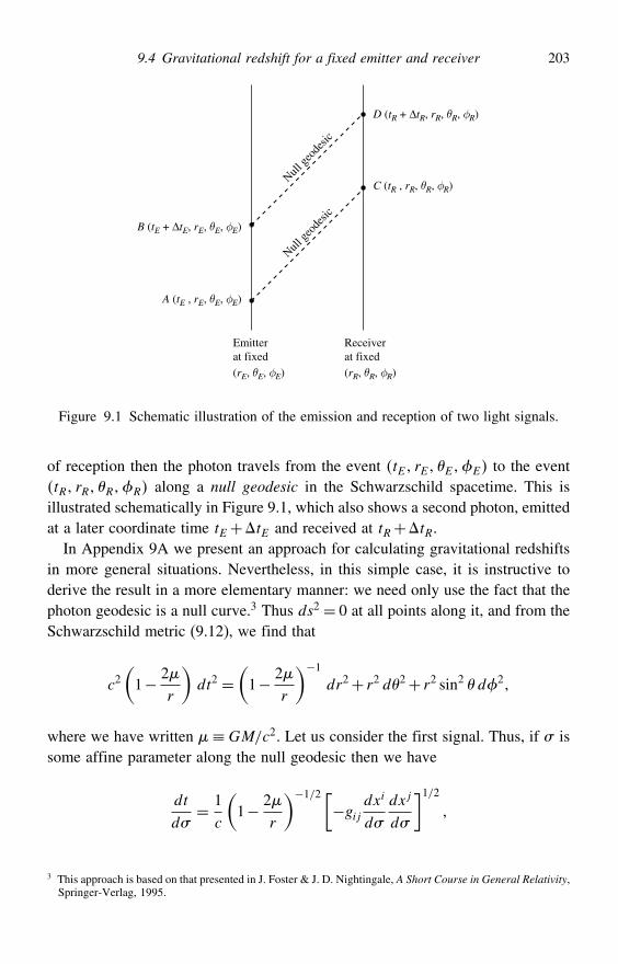
9.4 Gravitational redshift for a fixed emitter and receiver 203
B (tE + ∆tE, rE, θE, φE)
A (tE , rE, θE, φE)
C (tR , rR, θR, φR)
Emitterat fixed(rE, θE, φE)
Receiverat fixed(rR, θR, φR)
D (tR + ∆tR, rR, θR, φR)
Null ge
odes
ic
Null ge
odes
ic
Figure 9.1 Schematic illustration of the emission and reception of two light signals.
of reception then the photon travels from the event tE rE EE to the eventtR rR RR along a null geodesic in the Schwarzschild spacetime. This isillustrated schematically in Figure 9.1, which also shows a second photon, emittedat a later coordinate time tE+tE and received at tR+tR.In Appendix 9A we present an approach for calculating gravitational redshifts
in more general situations. Nevertheless, in this simple case, it is instructive toderive the result in a more elementary manner: we need only use the fact that thephoton geodesic is a null curve.3 Thus ds2 = 0 at all points along it, and from theSchwarzschild metric (9.12), we find that
c2(1− 2
r
)dt2 =
(1− 2
r
)−1dr2+ r2 d2+ r2 sin2 d2
where we have written ≡GM/c2. Let us consider the first signal. Thus, if # issome affine parameter along the null geodesic then we have
dt
d#= 1
c
(1− 2
r
)−1/2 [−gij
dxi
d#
dxj
d#
]1/2
3 This approach is based on that presented in J. Foster & J. D. Nightingale, A Short Course in General Relativity,Springer-Verlag, 1995.
204 The Schwarzschild geometry
where as before we use the notation x= t r , the g are the componentsof the Schwarzschild metric and Latin indices run from 1 to 3. On integrating,we obtain
tR− tE =1c
∫ #R
#E
(1− 2
r
)−1/2 [−gij
dxi
d#
dxj
d#
]1/2d#
where #E is the value of # at emission and #R the value at reception. Theimportant thing to notice about this expression is that the integral on the right-hand side depends only on the path through space. Thus, for a spatially fixedemitter and receiver, tR− tE is the same for all signals sent. Thus the coordinatetime difference tE separating events A and B is equal to the coordinate timetR between events C and D,
tR = tE
Now let us consider the proper time intervals along the worldlines of the emitterand receiver between each pair of events. Along both the emitter’s and receiver’sworldlines, dr = d= d= 0. Thus, from the Schwarzschild line element (9.12),in both cases
c2 d2 ≡ ds2 = c2(1− 2
r
)dt2
Moreover, in each case r is constant along the worldline, so we can immediatelyintegrate this equation to obtain
E =(1− 2
rE
)1/2
tE and R =(1− 2
rR
)1/2
tR
Thus, since tR = tE, we find that
RE
=(1−2/rR1−2/rE
)1/2
which forms the basis of the formula for gravitational redshift. If we think of thetwo light signals as, for example, the two wavecrests of an electromagnetic wave,then it is clear that this ratio must also be the ratio of the period of the waveas observed by the receiver and emitter respectively. Thus the frequencies of thephoton as measured by each observer are related by
RE=[1−2GM/rEc
2
1−2GM/rRc2
]1/2 (9.13)
which shows that R < E if rR > rE. The photon redshift z is defined by
1+ z= R/E−1
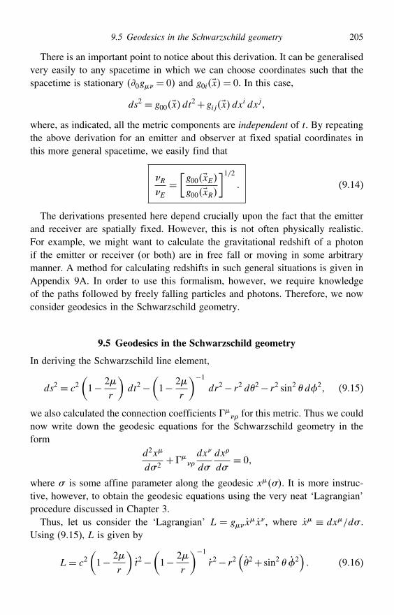
9.5 Geodesics in the Schwarzschild geometry 205
There is an important point to notice about this derivation. It can be generalisedvery easily to any spacetime in which we can choose coordinates such that thespacetime is stationary 0g = 0 and g0ix= 0. In this case,
ds2 = g00xdt2+gijxdxi dxjwhere, as indicated, all the metric components are independent of t. By repeatingthe above derivation for an emitter and observer at fixed spatial coordinates inthis more general spacetime, we easily find that
RE=[g00xEg00xR
]1/2 (9.14)
The derivations presented here depend crucially upon the fact that the emitterand receiver are spatially fixed. However, this is not often physically realistic.For example, we might want to calculate the gravitational redshift of a photonif the emitter or receiver (or both) are in free fall or moving in some arbitrarymanner. A method for calculating redshifts in such general situations is given inAppendix 9A. In order to use this formalism, however, we require knowledgeof the paths followed by freely falling particles and photons. Therefore, we nowconsider geodesics in the Schwarzschild geometry.
9.5 Geodesics in the Schwarzschild geometry
In deriving the Schwarzschild line element,
ds2 = c2(1− 2
r
)dt2−
(1− 2
r
)−1dr2− r2 d2− r2 sin2 d2 (9.15)
we also calculated the connection coefficients for this metric. Thus we could
now write down the geodesic equations for the Schwarzschild geometry in theform
d2x
d#2+
dx
d#
dx
d#= 0
where # is some affine parameter along the geodesic x#. It is more instruc-tive, however, to obtain the geodesic equations using the very neat ‘Lagrangian’procedure discussed in Chapter 3.
Thus, let us consider the ‘Lagrangian’ L = gxx, where x ≡ dx/d# .
Using (9.15), L is given by
L= c2(1− 2
r
)t2−
(1− 2
r
)−1r2− r2
(2+ sin2 2
) (9.16)
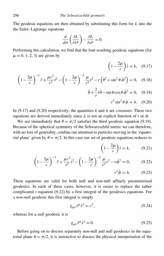
206 The Schwarzschild geometry
The geodesic equations are then obtained by substituting this form for L into thethe Euler–Lagrange equations
d
d#
(L
x
)− L
x= 0
Performing this calculation, we find that the four resulting geodesic equations (for= 0123) are given by (
1− 2r
)t = k (9.17)(
1− 2r
)−1r+ c2
r2t2−
(1− 2
r
)−2
r2r2− r
(2+ sin2 2
)= 0 (9.18)
+ 2rr− sin cos 2 = 0 (9.19)
r2 sin2 = h (9.20)
In (9.17) and (9.20) respectively, the quantities k and h are constants. These twoequations are derived immediately since L is not an explicit function of t or .
We see immediately that = /2 satisfies the third geodesic equation (9.19).Because of the spherical symmetry of the Schwarzschild metric we can therefore,with no loss of generality, confine our attention to particles moving in the ‘equato-rial plane’ given by =/2. In this case our set of geodesic equations reduces to(
1− 2r
)t = k (9.21)(
1− 2r
)−1r+ c2
r2t2−
(1− 2
r
)−2
r2r2− r2 = 0 (9.22)
r2 = h (9.23)
These equations are valid for both null and non-null affinely parameterisedgeodesics. In each of these cases, however, it is easier to replace the rathercomplicated r-equation (9.22) by a first integral of the geodesics equations. Fora non-null geodesic this first integral is simply
gxx = c2 (9.24)
whereas for a null geodesic it is
gxx = 0 (9.25)
Before going on to discuss separately non-null and null geodesics in the equa-torial plane = /2, it is instructive to discuss the physical interpretation of the
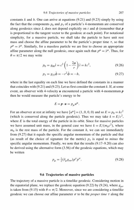
9.6 Trajectories of massive particles 207
constants k and h. One can arrive at equations (9.21) and (9.23) simply by usingthe fact that the components p0 and p3 of a particle’s 4-momentum are conservedalong geodesics since L does not depend explicitly on t and (remember that pis proportional to the tangent vector to the geodesic at each point). For notationalsimplicity, for a massive particle, we shall take the particle to have unit restmass and choose the affine parameter to be the particle’s proper time , so thatp = x. Similarly, for a massless particle we are free to choose an appropriateaffine parameter along the null geodesic, once again such that p = x. Thus, for = /2 we may write
p0 = g00 t = c2(1− 2
r
)t = kc2 (9.26)
p3 = g33=−r2=−h (9.27)
where in the last equality on each line we have defined the constants in a mannerthat coincides with (9.21) and (9.23). Let us first consider the constant k. If, at someevent, an observer with 4-velocity u encountered a particle with 4-momemtum pthen he would measure the particle’s energy to be
E = p ·u= pu
For an observer at rest at infinity we have u= 1000 and so E = p0 = kc2
(which is conserved along the particle geodesic). Thus we may take k = E/c2,where E is the total energy of the particle in its orbit. Since for massive particleswe have assumed unit mass, in the general case we have k = E/m0c
2, wherem0 is the rest mass of the particle. For the constant h, we can see immediatelyfrom (9.27) that it equals the specific angular momentum of the particle and that(as result of the choice of signature for the metric) p3 is equal to minus thespecific angular momentum. Finally, we note that the results (9.17–9.20) can alsobe derived using the alternative form (3.56) of the geodesic equations, which maybe written
p = 12g#p
p# (9.28)
9.6 Trajectories of massive particles
The trajectory of a massive particle is a timelike geodesic. Considering motion inthe equatorial plane, we replace the geodesic equation (9.22) by (9.24), where gis taken from (9.15) with =/2. Moreover, since we are considering a timelikegeodesic we can choose our affine parameter # to be the proper time along the
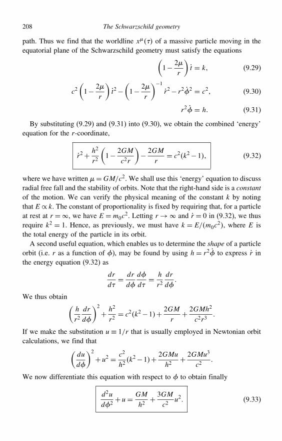
208 The Schwarzschild geometry
path. Thus we find that the worldline x of a massive particle moving in theequatorial plane of the Schwarzschild geometry must satisfy the equations(
1− 2r
)t = k (9.29)
c2(1− 2
r
)t2−
(1− 2
r
)−1r2− r22 = c2 (9.30)
r2 = h (9.31)
By substituting (9.29) and (9.31) into (9.30), we obtain the combined ‘energy’equation for the r-coordinate,
r2+ h2
r2
(1− 2GM
c2r
)− 2GM
r= c2k2−1 (9.32)
where we have written =GM/c2. We shall use this ‘energy’ equation to discussradial free fall and the stability of orbits. Note that the right-hand side is a constantof the motion. We can verify the physical meaning of the constant k by notingthat E ∝ k. The constant of proportionality is fixed by requiring that, for a particleat rest at r =, we have E =m0c
2. Letting r→ and r = 0 in (9.32), we thusrequire k2 = 1. Hence, as previously, we must have k = E/m0c
2, where E isthe total energy of the particle in its orbit.
A second useful equation, which enables us to determine the shape of a particleorbit (i.e. r as a function of ), may be found by using h= r2 to express r inthe energy equation (9.32) as
dr
d= dr
d
d
d= h
r2dr
d
We thus obtain(h
r2dr
d
)2
+ h2
r2= c2k2−1+ 2GM
r+ 2GMh2
c2r3
If we make the substitution u≡ 1/r that is usually employed in Newtonian orbitcalculations, we find that(
du
d
)2
+u2 = c2
h2k2−1+ 2GMu
h2+ 2GMu3
c2
We now differentiate this equation with respect to to obtain finally
d2u
d2+u= GM
h2+ 3GM
c2u2 (9.33)
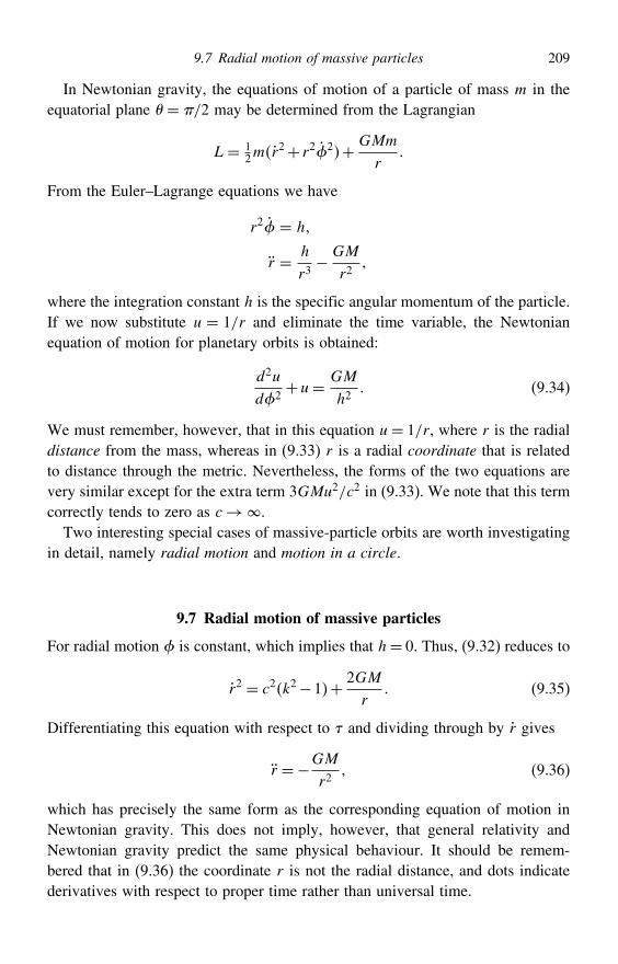
9.7 Radial motion of massive particles 209
In Newtonian gravity, the equations of motion of a particle of mass m in theequatorial plane = /2 may be determined from the Lagrangian
L= 12mr2+ r22+ GMm
r
From the Euler–Lagrange equations we have
r2 = h
r = h
r3− GM
r2
where the integration constant h is the specific angular momentum of the particle.If we now substitute u = 1/r and eliminate the time variable, the Newtonianequation of motion for planetary orbits is obtained:
d2u
d2+u= GM
h2 (9.34)
We must remember, however, that in this equation u= 1/r, where r is the radialdistance from the mass, whereas in (9.33) r is a radial coordinate that is relatedto distance through the metric. Nevertheless, the forms of the two equations arevery similar except for the extra term 3GMu2/c2 in (9.33). We note that this termcorrectly tends to zero as c→.
Two interesting special cases of massive-particle orbits are worth investigatingin detail, namely radial motion and motion in a circle.
9.7 Radial motion of massive particles
For radial motion is constant, which implies that h= 0. Thus, (9.32) reduces to
r2 = c2k2−1+ 2GM
r (9.35)
Differentiating this equation with respect to and dividing through by r gives
r =−GM
r2 (9.36)
which has precisely the same form as the corresponding equation of motion inNewtonian gravity. This does not imply, however, that general relativity andNewtonian gravity predict the same physical behaviour. It should be remem-bered that in (9.36) the coordinate r is not the radial distance, and dots indicatederivatives with respect to proper time rather than universal time.
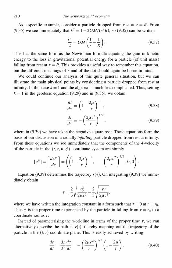
210 The Schwarzschild geometry
As a specific example, consider a particle dropped from rest at r = R. From(9.35) we see immediately that k2 = 1−2GM/c2R, so (9.35) can be written
r2
2=GM
(1r− 1R
) (9.37)
This has the same form as the Newtonian formula equating the gain in kineticenergy to the loss in gravitational potential energy for a particle (of unit mass)falling from rest at r = R. This provides a useful way to remember this equation,but the different meanings of r and of the dot should again be borne in mind.
We could continue our analysis of this quite general situation, but we canillustrate the main physical points by considering a particle dropped from rest atinfinity. In this case k= 1 and the algebra is much less complicated. Thus, settingk= 1 in the geodesic equation (9.29) and in (9.35), we obtain
dt
d=(1− 2
r
)−1 (9.38)
dr
d= −
(2c2
r
)1/2
(9.39)
where in (9.39) we have taken the negative square root. These equations form thebasis of our discussion of a radially infalling particle dropped from rest at infinity.From these equations we see immediately that the components of the 4-velocityof the particle in the t r coordinate system are simply
u≡[dx
d
]=((
1− 2r
)−1 −
(2c2
r
)1/2
00
)
Equation (9.39) determines the trajectory r. On integrating (9.39) we imme-diately obtain
= 23
√r30
2c2− 2
3
√r3
2c2
where we have written the integration constant in a form such that = 0 at r = r0.Thus is the proper time experienced by the particle in falling from r = r0 to acoordinate radius r .
Instead of parameterising the worldline in terms of the proper time , we canalternatively describe the path as rt, thereby mapping out the trajectory of theparticle in the t r coordinate plane. This is easily achieved by writing
dr
dt= dr
d
d
dt=−
(2c2
r
)1/2(1− 2
r
) (9.40)
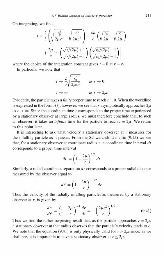
9.7 Radial motion of massive particles 211
On integrating, we find
t = 23
⎛⎝√ r302c2
−√
r3
2c2
⎞⎠+ 4c
(√r02−√
r
2
)
+ 2c
ln
∣∣∣∣∣(√
r/2+1√r/2−1
)(√r0/2−1√r0/2+1
)∣∣∣∣∣ where the choice of the integration constant gives t = 0 at r = r0.In particular we note that
→ 23
√r30
2c2as r→ 0
t→ as r→ 2
Evidently, the particle takes a finite proper time to reach r = 0. When the worldlineis expressed in the form rt, however, we see that r asymptotically approaches 2as t→. Since the coordinate time t corresponds to the proper time experiencedby a stationary observer at large radius, we must therefore conclude that, to suchan observer, it takes an infinite time for the particle to reach r = 2. We returnto this point later.
It is interesting to ask what velocity a stationary observer at r measures forthe infalling particle as it passes. From the Schwarzschild metric (9.15) we seethat, for a stationary observer at coordinate radius r, a coordinate time interval dtcorresponds to a proper time interval
dt′ =(1− 2
r
)1/2
dt
Similarly, a radial coordinate separation dr corresponds to a proper radial distancemeasured by the observer equal to
dr ′ =(1− 2
r
)−1/2dr
Thus the velocity of the radially infalling particle, as measured by a stationaryobserver at r , is given by
dr ′
dt′=(1− 2
r
)−1 drdt=−
(2c2
r
)1/2
(9.41)
Thus we find the rather surprising result that, as the particle approaches r = 2,a stationary observer at that radius observes that the particle’s velocity tends to c.We note that the equation (9.41) is only physically valid for r > 2 since, as weshall see, it is impossible to have a stationary observer at r ≤ 2.
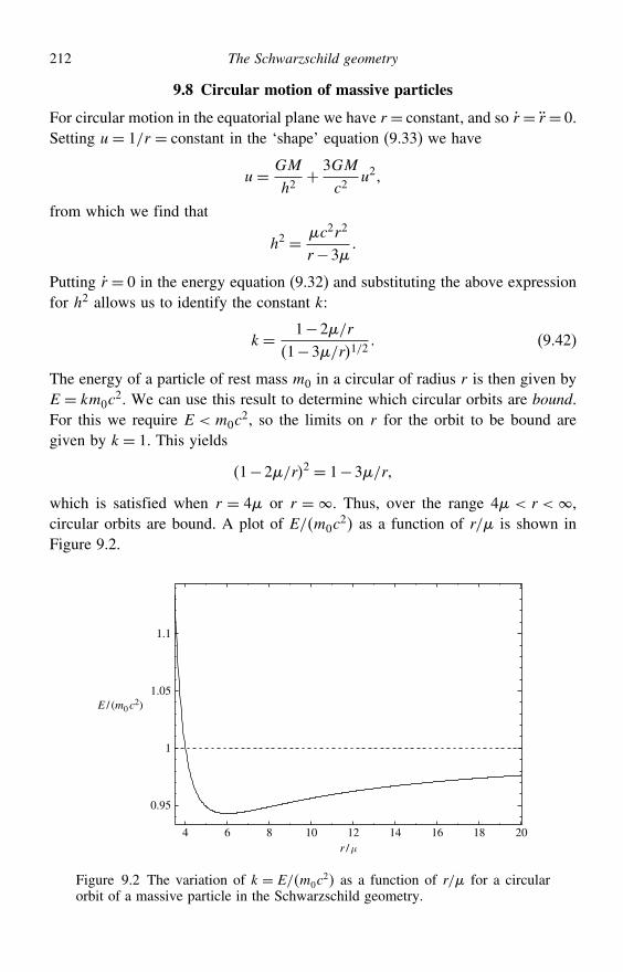
212 The Schwarzschild geometry
9.8 Circular motion of massive particles
For circular motion in the equatorial plane we have r = constant, and so r = r = 0.Setting u= 1/r = constant in the ‘shape’ equation (9.33) we have
u= GM
h2+ 3GM
c2u2
from which we find that
h2 = c2r2
r−3
Putting r = 0 in the energy equation (9.32) and substituting the above expressionfor h2 allows us to identify the constant k:
k= 1−2/r1−3/r1/2
(9.42)
The energy of a particle of rest mass m0 in a circular of radius r is then given byE = km0c
2. We can use this result to determine which circular orbits are bound.For this we require E < m0c
2, so the limits on r for the orbit to be bound aregiven by k= 1. This yields
1−2/r2 = 1−3/r
which is satisfied when r = 4 or r = . Thus, over the range 4 < r < ,circular orbits are bound. A plot of E/m0c
2 as a function of r/ is shown inFigure 9.2.
4
0.95
1
1.05
1.1
6 8 10 12r /µ
14 16 18 20
E / (m0 c2)
Figure 9.2 The variation of k = E/m0c2 as a function of r/ for a circular
orbit of a massive particle in the Schwarzschild geometry.
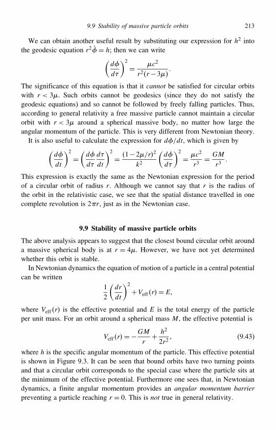
9.9 Stability of massive particle orbits 213
We can obtain another useful result by substituting our expression for h2 intothe geodesic equation r2= h; then we can write(
d
d
)2
= c2
r2r−3
The significance of this equation is that it cannot be satisfied for circular orbitswith r < 3. Such orbits cannot be geodesics (since they do not satisfy thegeodesic equations) and so cannot be followed by freely falling particles. Thus,according to general relativity a free massive particle cannot maintain a circularorbit with r < 3 around a spherical massive body, no matter how large theangular momentum of the particle. This is very different from Newtonian theory.
It is also useful to calculate the expression for d/dt, which is given by(d
dt
)2
=(d
d
d
dt
)2
= 1−2/r2
k2
(d
d
)2
= c2
r3= GM
r3
This expression is exactly the same as the Newtonian expression for the periodof a circular orbit of radius r. Although we cannot say that r is the radius ofthe orbit in the relativistic case, we see that the spatial distance travelled in onecomplete revolution is 2r, just as in the Newtonian case.
9.9 Stability of massive particle orbits
The above analysis appears to suggest that the closest bound circular orbit arounda massive spherical body is at r = 4. However, we have not yet determinedwhether this orbit is stable.
In Newtonian dynamics the equation of motion of a particle in a central potentialcan be written
12
(dr
dt
)2
+Veffr= E
where Veffr is the effective potential and E is the total energy of the particleper unit mass. For an orbit around a spherical mass M , the effective potential is
Veffr=−GM
r+ h2
2r2 (9.43)
where h is the specific angular momentum of the particle. This effective potentialis shown in Figure 9.3. It can be seen that bound orbits have two turning pointsand that a circular orbit corresponds to the special case where the particle sits atthe minimum of the effective potential. Furthermore one sees that, in Newtoniandynamics, a finite angular momentum provides an angular momentum barrierpreventing a particle reaching r = 0. This is not true in general relativity.
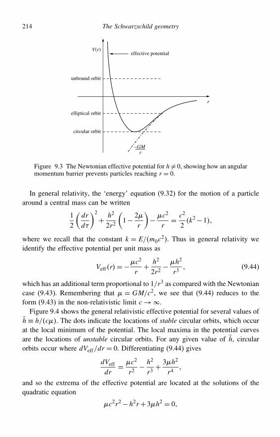
214 The Schwarzschild geometry
effective potential
r
unbound orbit
elliptical orbit
circular orbit
V(r)
–GMr
Figure 9.3 The Newtonian effective potential for h = 0, showing how an angularmomentum barrier prevents particles reaching r = 0.
In general relativity, the ‘energy’ equation (9.32) for the motion of a particlearound a central mass can be written
12
(dr
d
)2
+ h2
2r2
(1− 2
r
)− c2
r= c2
2k2−1
where we recall that the constant k = E/m0c2. Thus in general relativity we
identify the effective potential per unit mass as
Veffr=−c2
r+ h2
2r2− h2
r3 (9.44)
which has an additional term proportional to 1/r3 as compared with the Newtoniancase (9.43). Remembering that = GM/c2, we see that (9.44) reduces to theform (9.43) in the non-relativistic limit c→.
Figure 9.4 shows the general relativistic effective potential for several values ofh≡ h/c. The dots indicate the locations of stable circular orbits, which occurat the local minimum of the potential. The local maxima in the potential curvesare the locations of unstable circular orbits. For any given value of h, circularorbits occur where dVeff/dr = 0. Differentiating (9.44) gives
dVeff
dr= c2
r2− h2
r3+ 3h2
r4
and so the extrema of the effective potential are located at the solutions of thequadratic equation
c2r2−h2r+3h2 = 0
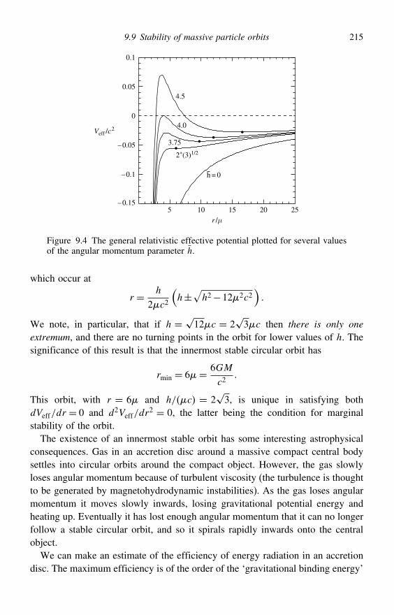
9.9 Stability of massive particle orbits 215
5
2*(3)1/2
Veff /c2
3.75
4.0
4.5
–0.15
–0.1
–0.05
0
0.05
0.1
r /µ10 15 20 25
h = 0
Figure 9.4 The general relativistic effective potential plotted for several valuesof the angular momentum parameter h.
which occur at
r = h
2c2
(h±
√h2−122c2
)
We note, in particular, that if h = √12c = 2√3c then there is only one
extremum, and there are no turning points in the orbit for lower values of h. Thesignificance of this result is that the innermost stable circular orbit has
rmin = 6= 6GM
c2
This orbit, with r = 6 and h/c = 2√3, is unique in satisfying both
dVeff/dr = 0 and d2Veff/dr2 = 0, the latter being the condition for marginal
stability of the orbit.The existence of an innermost stable orbit has some interesting astrophysical
consequences. Gas in an accretion disc around a massive compact central bodysettles into circular orbits around the compact object. However, the gas slowlyloses angular momentum because of turbulent viscosity (the turbulence is thoughtto be generated by magnetohydrodynamic instabilities). As the gas loses angularmomentum it moves slowly inwards, losing gravitational potential energy andheating up. Eventually it has lost enough angular momentum that it can no longerfollow a stable circular orbit, and so it spirals rapidly inwards onto the centralobject.
We can make an estimate of the efficiency of energy radiation in an accretiondisc. The maximum efficiency is of the order of the ‘gravitational binding energy’
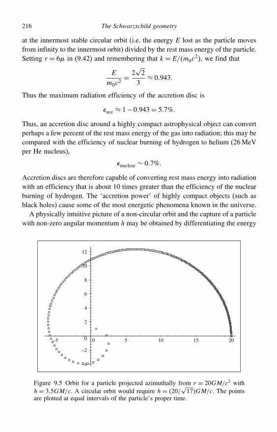
216 The Schwarzschild geometry
at the innermost stable circular orbit (i.e. the energy E lost as the particle movesfrom infinity to the innermost orbit) divided by the rest mass energy of the particle.Setting r = 6 in (9.42) and remembering that k= E/m0c
2, we find that
E
m0c2= 2
√2
3≈ 0943
Thus the maximum radiation efficiency of the accretion disc is
acc ≈ 1−0943= 57%
Thus, an accretion disc around a highly compact astrophysical object can convertperhaps a few percent of the rest mass energy of the gas into radiation; this may becompared with the efficiency of nuclear burning of hydrogen to helium (26MeVper He nucleus),
nuclear ∼ 07%
Accretion discs are therefore capable of converting rest mass energy into radiationwith an efficiency that is about 10 times greater than the efficiency of the nuclearburning of hydrogen. The ‘accretion power’ of highly compact objects (such asblack holes) cause some of the most energetic phenomena known in the universe.
A physically intuitive picture of a non-circular orbit and the capture of a particlewith non-zero angular momentum h may be obtained by differentiating the energy
–4
–2
0
2
4
6
8
10
12
–5 0 5 10 15 20
Figure 9.5 Orbit for a particle projected azimuthally from r = 20GM/c2 withh= 35GM/c. A circular orbit would require h= 20/
√17GM/c. The points
are plotted at equal intervals of the particle’s proper time.
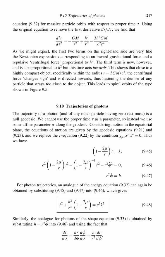
9.10 Trajectories of photons 217
equation (9.32) for massive particle orbits with respect to proper time . Usingthe original equation to remove the first derivative dr/d, we find that
d2r
d2=−GM
r2+ h2
r3− 3h2GM
c2r4
As we might expect, the first two terms on the right-hand side are very likethe Newtonian expressions corresponding to an inward gravitational force and arepulsive ‘centrifugal force’ proportional to h2. The third term is new, however,and is also proportional to h2 but this time acts inwards. This shows that close to ahighly compact object, specifically within the radius r = 3GM/c2, the centrifugalforce ‘changes sign’ and is directed inwards, thus hastening the demise of anyparticle that strays too close to the object. This leads to spiral orbits of the typeshown in Figure 9.5.
9.10 Trajectories of photons
The trajectory of a photon (and of any other particle having zero rest mass) is anull geodesic. We cannot use the proper time as a parameter, so instead we usesome affine parameter # along the geodesic. Considering motion in the equatorialplane, the equations of motion are given by the geodesic equations (9.21) and(9.23), and we replace the r-equation (9.22) by the condition gx
x = 0. Thuswe have (
1− 2r
)t = k (9.45)
c2(1− 2
r
)t2−
(1− 2
r
)−1r2− r22 = 0 (9.46)
r2 = h (9.47)
For photon trajectories, an analogue of the energy equation (9.32) can again beobtained by substituting (9.45) and (9.47) into (9.46), which gives
r2+ h2
r2
(1− 2
r
)= c2k2 (9.48)
Similarly, the analogue for photons of the shape equation (9.33) is obtained bysubstituting h= r2 into (9.46) and using the fact that
dr
d#= dr
d
d
d#= h
r2dr
d
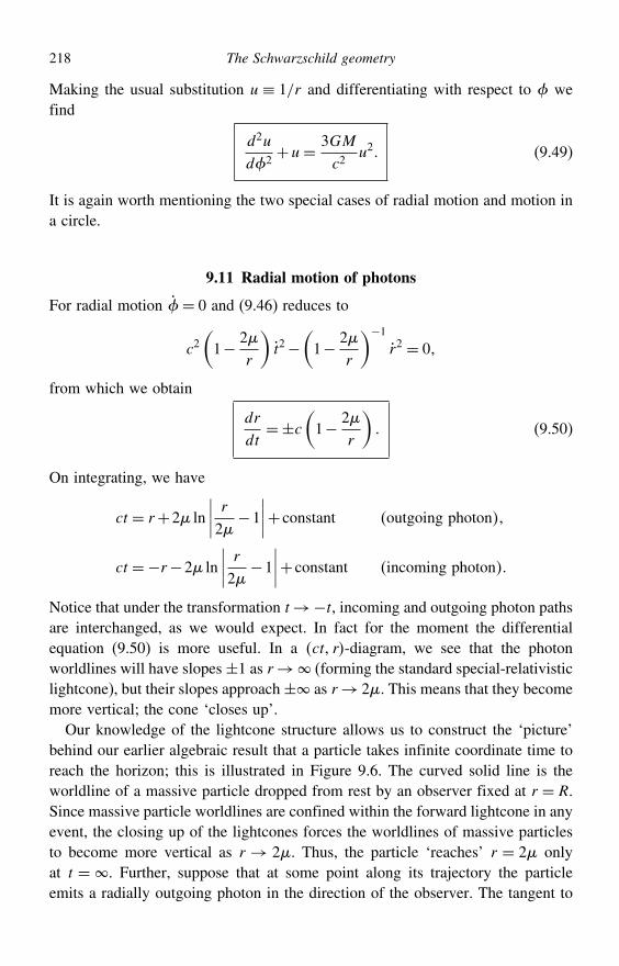
218 The Schwarzschild geometry
Making the usual substitution u ≡ 1/r and differentiating with respect to wefind
d2u
d2+u= 3GM
c2u2 (9.49)
It is again worth mentioning the two special cases of radial motion and motion ina circle.
9.11 Radial motion of photons
For radial motion = 0 and (9.46) reduces to
c2(1− 2
r
)t2−
(1− 2
r
)−1r2 = 0
from which we obtain
dr
dt=±c
(1− 2
r
) (9.50)
On integrating, we have
ct = r+2 ln
∣∣∣∣ r2 −1
∣∣∣∣+ constant outgoing photon
ct =−r−2 ln
∣∣∣∣ r2 −1
∣∣∣∣+ constant incoming photon
Notice that under the transformation t→−t, incoming and outgoing photon pathsare interchanged, as we would expect. In fact for the moment the differentialequation (9.50) is more useful. In a ct r-diagram, we see that the photonworldlines will have slopes±1 as r→ (forming the standard special-relativisticlightcone), but their slopes approach± as r→ 2. This means that they becomemore vertical; the cone ‘closes up’.
Our knowledge of the lightcone structure allows us to construct the ‘picture’behind our earlier algebraic result that a particle takes infinite coordinate time toreach the horizon; this is illustrated in Figure 9.6. The curved solid line is theworldline of a massive particle dropped from rest by an observer fixed at r = R.Since massive particle worldlines are confined within the forward lightcone in anyevent, the closing up of the lightcones forces the worldlines of massive particlesto become more vertical as r → 2. Thus, the particle ‘reaches’ r = 2 onlyat t = . Further, suppose that at some point along its trajectory the particleemits a radially outgoing photon in the direction of the observer. The tangent to
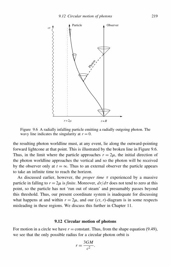
9.12 Circular motion of photons 219
r = Rr = 2µ
ctObserverParticle
Phot
on
Figure 9.6 A radially infalling particle emitting a radially outgoing photon. Thewavy line indicates the singularity at r = 0.
the resulting photon worldline must, at any event, lie along the outward-pointingforward lightcone at that point. This is illustrated by the broken line in Figure 9.6.Thus, in the limit where the particle approaches r = 2, the initial direction ofthe photon worldline approaches the vertical and so the photon will be receivedby the observer only at t =. Thus to an external observer the particle appearsto take an infinite time to reach the horizon.
As discussed earlier, however, the proper time experienced by a massiveparticle in falling to r = 2 is finite. Moreover, dr/d does not tend to zero at thispoint, so the particle has not ‘run out of steam’ and presumably passes beyondthis threshold. Thus, our present coordinate system is inadequate for discussingwhat happens at and within r = 2, and our ct r-diagram is in some respectsmisleading in these regions. We discuss this further in Chapter 11.
9.12 Circular motion of photons
For motion in a circle we have r = constant. Thus, from the shape equation (9.49),we see that the only possible radius for a circular photon orbit is
r = 3GM
c2
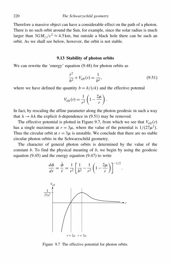
220 The Schwarzschild geometry
Therefore a massive object can have a considerable effect on the path of a photon.There is no such orbit around the Sun, for example, since the solar radius is muchlarger than 3GM/c2 ≈ 45km, but outside a black hole there can be such anorbit. As we shall see below, however, the orbit is not stable.
9.13 Stability of photon orbits
We can rewrite the ‘energy’ equation (9.48) for photon orbits as
r2
h2+Veffr=
1b2
(9.51)
where we have defined the quantity b = h/ck and the effective potental
Veffr=1r2
(1− 2
r
)
In fact, by rescaling the affine parameter along the photon geodesic in such a waythat → h the explicit h-dependence in (9.51) may be removed.
The effective potential is plotted in Figure 9.7, from which we see that Veffr
has a single maximum at r = 3, where the value of the potential is 1/272.Thus the circular orbit at r = 3 is unstable. We conclude that there are no stablecircular photon orbits in the Schwarzschild geometry.
The character of general photon orbits is determined by the value of theconstant b. To find the physical meaning of b, we begin by using the geodesicequation (9.45) and the energy equation (9.47) to write
d
dr=
r= 1
r2
[1b2− 1r2
(1− 2
r
)]−1/2
r
Veff
r = 2µ r = 3µ
27µ21
Figure 9.7 The effective potential for photon orbits.
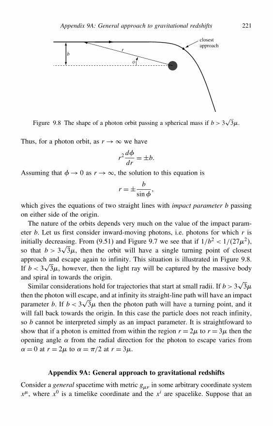
Appendix 9A: General approach to gravitational redshifts 221
br
φ
closestapproach
Figure 9.8 The shape of a photon orbit passing a spherical mass if b > 3√3.
Thus, for a photon orbit, as r→ we have
r2d
dr=±b
Assuming that → 0 as r→, the solution to this equation is
r =± b
sin
which gives the equations of two straight lines with impact parameter b passingon either side of the origin.
The nature of the orbits depends very much on the value of the impact param-eter b. Let us first consider inward-moving photons, i.e. photons for which r isinitially decreasing. From (9.51) and Figure 9.7 we see that if 1/b2 < 1/272,so that b > 3
√3, then the orbit will have a single turning point of closest
approach and escape again to infinity. This situation is illustrated in Figure 9.8.If b < 3
√3, however, then the light ray will be captured by the massive body
and spiral in towards the origin.Similar considerations hold for trajectories that start at small radii. If b> 3
√3
then the photon will escape, and at infinity its straight-line path will have an impactparameter b. If b < 3
√3 then the photon path will have a turning point, and it
will fall back towards the origin. In this case the particle does not reach infinity,so b cannot be interpreted simply as an impact parameter. It is straightfoward toshow that if a photon is emitted from within the region r = 2 to r = 3 then theopening angle from the radial direction for the photon to escape varies from= 0 at r = 2 to = /2 at r = 3.
Appendix 9A: General approach to gravitational redshifts
Consider a general spacetime with metric g in some arbitrary coordinate systemx, where x0 is a timelike coordinate and the xi are spacelike. Suppose that an
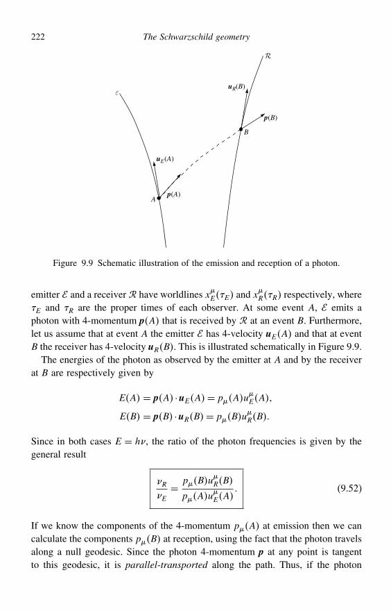
222 The Schwarzschild geometry
B
Ap(A)
p(B)
uR(B)
uE(A)
ε
Figure 9.9 Schematic illustration of the emission and reception of a photon.
emitter and a receiver have worldlines xEE and xRR respectively, where
E and R are the proper times of each observer. At some event A, emits aphoton with 4-momentum pA that is received by at an event B. Furthermore,let us assume that at event A the emitter has 4-velocity uEA and that at eventB the receiver has 4-velocity uRB. This is illustrated schematically in Figure 9.9.
The energies of the photon as observed by the emitter at A and by the receiverat B are respectively given by
EA = pA ·uEA= pAuEA
EB = pB ·uRB= pBuRB
Since in both cases E = h, the ratio of the photon frequencies is given by thegeneral result
RE= pBu
RB
pAuEA
(9.52)
If we know the components of the 4-momentum pA at emission then we cancalculate the components pB at reception, using the fact that the photon travelsalong a null geodesic. Since the photon 4-momentum p at any point is tangentto this geodesic, it is parallel-transported along the path. Thus, if the photon
Appendix 9A: General approach to gravitational redshifts 223
geodesic x# is described in terms of some affine parameter # then
dp
d#−
pdx
d#= 0
Moreover, since p is tangent to the geodesics, we can choose the affine parameter# so that p = dx/d# , in which case
dp
d#=
pp
It is also worth remembering that a first integral of the equation for a photongeodesic, which can prove very useful, is
pp = 0 (9.53)
Let us now examine some special cases of the general formula (9.52). Webegin by considering the case in which both the emitter and the receiver have fixed spatial coordinates. Thus, for i = 123 the spatial components oftheir 4-velocities are
uiE ≡dxiEdE
= 0 and uiR ≡dxiRdR
= 0
Moreover, in each case, the squared length of the 4-velocity is guu = c2. In
our situation, this reduces to g00u02 = c2, so we find that
u0 = c
g001/2
Hence the formula (9.52) reduces to
RE= p0B
p0A
[g00A
g00B
]1/2 (9.54)
Let us now make the additional assumption that the metric is stationary in ourchosen cooordinate system, i.e.
0g = 0
Thus, the metric components g cannot depend explicitly on the coordinate x0.As shown in Section 3.19, this means that the zeroth covariant component of thetangent vector is constant along an affinely parameterised geodesic. Since thephoton 4-momentum is simply proportional to the tangent vector, this means that
224 The Schwarzschild geometry
p0 is constant along the photon’s geodesic. Thus, in this case, (9.54) reducesfurther to
RE=[g00A
g00B
]1/2 (9.55)
and we have recovered the result (9.14) derived earlier.
Exercises
9.1 Show that surfaces of constant t and r in the general isotropic metric (9.3) havesurface area 4r2.
9.2 For the general static isotropic metric (9.4), show that the off-diagonal components ofthe Ricci tensorR are zero and that the diagonal components are given by (9.8–9.11).
9.3 The Schwarzschild line element is
ds2 = c2(1− 2
r
)dt2−
(1− 2
r
)−1dr2− r2 d2− r2 sin2 d2
By considering the ‘Lagrangian’ L= gxx, where the dots denote differentiation
with respect to an affine parameter , calculate the connection coefficients # .
Hence verify that the geodesic equations are given by (9.17–9.20).9.4 Derive the results (9.17–9.20) using the alternative form (9.28) of the geodesic
equations.9.5 Calculate the connection coefficients and the Ricci tensor for the general isotropic
metric (9.3). Hence prove Birkoff’s theorem.9.6 Use Birkhoff’s theorem to show that a particle inside a spherical shell of matter
experiences no gravitational force.9.7 Show that the ‘Lemaitre’ line element
ds2 = c2 dw2− 49
[9
2z− cw
]2/3dz2−
[92z− cw2
]2/3d2
where d2 = d2+ sin2 d2, describes the Schwarzschild geometry. Show thatobservers with fixed spatial coordinates z are in free fall and had zero velocityat infinity, and that the proper time of such observers is w.
9.8 For a general stationary spacetime with line element
ds2 = g00xdt2+gijxdxi dxjshow that, for a fixed emitter and receiver, the ratio of the received photon frequencyto the emitted frequency is
RE=[g00xEg00xR
]1/2
where xE and xR are the fixed spatial coordinates of the emitter and receiverrespectively.
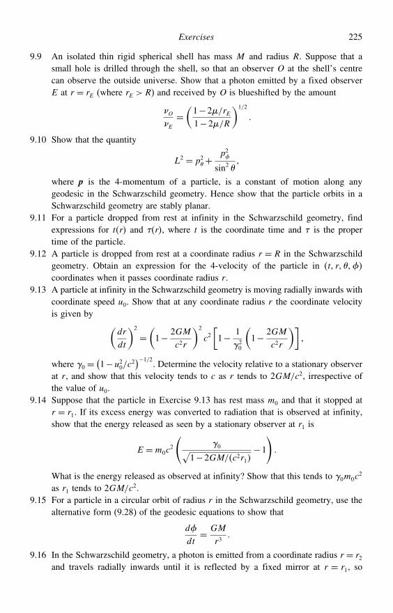
Exercises 225
9.9 An isolated thin rigid spherical shell has mass M and radius R. Suppose that asmall hole is drilled through the shell, so that an observer O at the shell’s centrecan observe the outside universe. Show that a photon emitted by a fixed observerE at r = rE (where rE > R) and received by O is blueshifted by the amount
OE=(1−2/rE1−2/R
)1/2
9.10 Show that the quantity
L2 = p2+
p2
sin2
where p is the 4-momentum of a particle, is a constant of motion along anygeodesic in the Schwarzschild geometry. Hence show that the particle orbits in aSchwarzschild geometry are stably planar.
9.11 For a particle dropped from rest at infinity in the Schwarzschild geometry, findexpressions for tr and r, where t is the coordinate time and is the propertime of the particle.
9.12 A particle is dropped from rest at a coordinate radius r = R in the Schwarzschildgeometry. Obtain an expression for the 4-velocity of the particle in t r
coordinates when it passes coordinate radius r.9.13 A particle at infinity in the Schwarzschild geometry is moving radially inwards with
coordinate speed u0. Show that at any coordinate radius r the coordinate velocityis given by (
dr
dt
)2
=(1− 2GM
c2r
)2
c2[1− 1
20
(1− 2GM
c2r
)]
where 0 =(1−u2
0/c2)−1/2
. Determine the velocity relative to a stationary observerat r, and show that this velocity tends to c as r tends to 2GM/c2, irrespective ofthe value of u0.
9.14 Suppose that the particle in Exercise 9.13 has rest mass m0 and that it stopped atr = r1. If its excess energy was converted to radiation that is observed at infinity,show that the energy released as seen by a stationary observer at r1 is
E =m0c2
(0√
1−2GM/c2r1−1
)
What is the energy released as observed at infinity? Show that this tends to 0m0c2
as r1 tends to 2GM/c2.9.15 For a particle in a circular orbit of radius r in the Schwarzschild geometry, use the
alternative form (9.28) of the geodesic equations to show that
d
dt= GM
r3
9.16 In the Schwarzschild geometry, a photon is emitted from a coordinate radius r = r2and travels radially inwards until it is reflected by a fixed mirror at r = r1, so
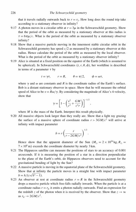
226 The Schwarzschild geometry
that it travels radially outwards back to r = r2. How long does the round trip takeaccording to a stationary observer in infinity?
9.17 A photon moves in a circular orbit at r = 3 in the Schwarzschild geometry. Showthat the period of the orbit as measured by a stationary observer at this radius is = 6/c. What is the period of the orbit as measured by a stationary observerinfinity?
9.18 Show that a massive particle moving in the innermost stable circular orbit in theSchwarzschild geometry has speed c/2 as measured by a stationary observer at thisradius. Hence calculate the period of the orbit as measured by the local observer.What is the period of the orbit as measured by a stationary observer infinity?
9.19 Alice is situated at a fixed position on the equator of the Earth (which is assumed tobe spherical). In Schwarzschild coordinates t r , her worldline is describedin terms of a parameter by
t = r = R = /2 =
where and are constants and R is the coordinate radius of the Earth’s surface.Bob is a distant stationary observer in space. Show that he will measure the orbitalspeed of Alice to be v=R/. By considering the magnitude of Alice’s 4-velocity,show that
=[1−
(v2
c2+ GM
c2r
)]−1/2
where M is the mass of the Earth. Interpret this result physically.9.20 All massive objects look larger than they really are. Show that a light ray grazing
the surface of a massive sphere of coordinate radius r > 3GM/c2 will arrive atinfinity with impact parameter
b = r
(r
r−2GM/c2
)1/2
Hence show that the apparent diameter of the Sun M = 2× 1030 kgR =7×10⁸ m exceeds the coordinate diameter by nearly 3 km.
9.21 The Hipparcos satellite can measure the positions of stars to an accuracy of 0.001arcseconds. If it is measuring the position of a star in a direction perpendicularto the plane of the Earth’s orbit, do Hipparcos observers need to account for thegravitational bending of light by the Sun?
9.22 A massive particle is moving in the equatorial plane of the Schwarzschild geometry.Show that at infinity the particle moves in a straight line with impact parameterb = h/c
√k2−1.
9.23 An observer at rest at coordinate radius r = R in the Schwarzschild geometrydrops a massive particle which free-falls radially inwards. When the particle is at acoordinate radius r = rE it emits a photon radially outwards. Find an expression forthe redshift z of the photon when it is received by the observer. Show that z→as rE → 2GM/c2.
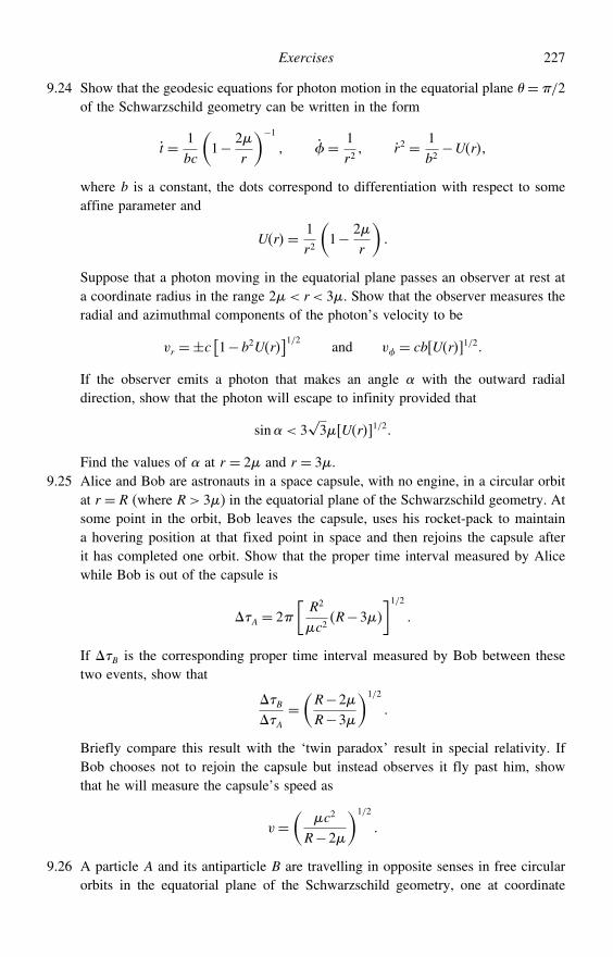
Exercises 227
9.24 Show that the geodesic equations for photon motion in the equatorial plane =/2of the Schwarzschild geometry can be written in the form
t = 1bc
(1− 2
r
)−1 = 1
r2 r2 = 1
b2−Ur
where b is a constant, the dots correspond to differentiation with respect to someaffine parameter and
Ur= 1r2
(1− 2
r
)
Suppose that a photon moving in the equatorial plane passes an observer at rest ata coordinate radius in the range 2< r < 3. Show that the observer measures theradial and azimuthmal components of the photon’s velocity to be
vr =±c[1−b2Ur
]1/2and v = cb Ur1/2
If the observer emits a photon that makes an angle with the outward radialdirection, show that the photon will escape to infinity provided that
sin < 3√3 Ur1/2
Find the values of at r = 2 and r = 3.9.25 Alice and Bob are astronauts in a space capsule, with no engine, in a circular orbit
at r = R (where R> 3) in the equatorial plane of the Schwarzschild geometry. Atsome point in the orbit, Bob leaves the capsule, uses his rocket-pack to maintaina hovering position at that fixed point in space and then rejoins the capsule afterit has completed one orbit. Show that the proper time interval measured by Alicewhile Bob is out of the capsule is
A = 2[R2
c2R−3
]1/2
If B is the corresponding proper time interval measured by Bob between thesetwo events, show that
BA
=(R−2R−3
)1/2
Briefly compare this result with the ‘twin paradox’ result in special relativity. IfBob chooses not to rejoin the capsule but instead observes it fly past him, showthat he will measure the capsule’s speed as
v=(
c2
R−2
)1/2
9.26 A particle A and its antiparticle B are travelling in opposite senses in free circularorbits in the equatorial plane of the Schwarzschild geometry, one at coordinate
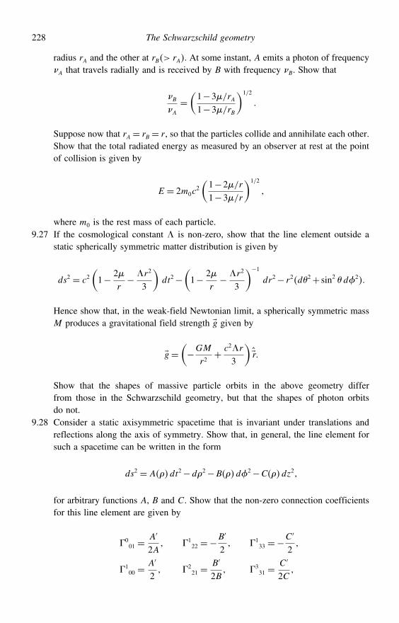
228 The Schwarzschild geometry
radius rA and the other at rB> rA. At some instant, A emits a photon of frequencyA that travels radially and is received by B with frequency B. Show that
BA=(1−3/rA1−3/rB
)1/2
Suppose now that rA = rB = r, so that the particles collide and annihilate each other.Show that the total radiated energy as measured by an observer at rest at the pointof collision is given by
E = 2m0c2
(1−2/r1−3/r
)1/2
where m0 is the rest mass of each particle.9.27 If the cosmological constant $ is non-zero, show that the line element outside a
static spherically symmetric matter distribution is given by
ds2 = c2(1− 2
r− $r2
3
)dt2−
(1− 2
r− $r2
3
)−1dr2− r2d2+ sin2 d2
Hence show that, in the weak-field Newtonian limit, a spherically symmetric massM produces a gravitational field strength g given by
g =(−GM
r2+ c2$r
3
)r
Show that the shapes of massive particle orbits in the above geometry differfrom those in the Schwarzschild geometry, but that the shapes of photon orbitsdo not.
9.28 Consider a static axisymmetric spacetime that is invariant under translations andreflections along the axis of symmetry. Show that, in general, the line element forsuch a spacetime can be written in the form
ds2 = Adt2−d2−Bd2−Cdz2
for arbitrary functions A, B and C. Show that the non-zero connection coefficientsfor this line element are given by
001 =
A′
2A 1
22 =−B′
2 1
33 =−C ′
2
100 =
A′
2 2
21 =B′
2B 3
31 =C ′
2C
Exercises 229
where the primes denote d/d. Hence show that the non-zero components of theRicci tensor are given by
R00 = −A′′
2+ A′
2
(A′
2A− B′
2B− C ′
2C
)
R11 =A′′
2A− A′2
4A2+ B′′
2B− B′2
4B2+ C ′′
2C− C ′2
4C2
R22 =B′′
2− B′
2
(B′
2B− A′
2A− C ′
2C
)
R33 =C ′′
2− C ′
2
(C ′
2C− A′
2A− B′
2B
)
9.29 Consider a static, infinitely long, cylindrically symmetric matter distribution ofconstant radius that is invariant to Lorentz boosts along the symmetry axis (a‘cosmic string’). Show that the line element outside the body can be written as
ds2 = c2 dt2−d2− +2 d2−dz2
where and are constants. For the case = 0, consider the spacelike surfacesdefined by t= constant and z= constant and calculate the circumference of a circleof constant coordinate radius in such a surface. Hence show that, for < 1, thegeometry on the spacelike surface is that of a two-dimensional cone embedded inthree-dimensional Euclidean space.
10
Experimental tests of general relativity
Most of the experimental tests of general relativity are based on the Schwarzschildgeometry in the region r > 2GM/c2. Some are based on the trajectories of massiveparticles and others on photon trajectories. Most of the ‘classic’ tests are in theweak-field limit, but more recent observations have begun to probe the morediscriminative strong-field regime. We will now discuss both these ‘classic’ exper-imental tests and some of the more recent findings and proposals. Some latertests are in fact more closely linked to the Kerr geometry (see Chapter 13), whichdescribes spacetime outside a rotating massive body, but the basic principles canstill be understood in terms of the simpler Schwarzschild geometry.
10.1 Precession of planetary orbits
For a general non-circular orbit in Newtonian theory the equation of motion is
d2u
d2+u= GM
h2
where u ≡ 1/r and h is the angular momentum per unit mass of the orbitingparticle. For a bound orbit, the equation has the solution
u= GM
h21+ e cos (10.1)
which describes an ellipse; the parameter e measures the ellipticity of the orbit.Thus, for example, we can draw the orbit of a planet around the Sun as inFigure 10.1. We can write the distance of closest approach (perihelion) as r1 =a1− e and the distance of furthest approach (aphelion) as r2 = a1+ e. Theequation of motion then requires that the semi-major axis is given by
a= h2
GM1− e2 (10.2)
230
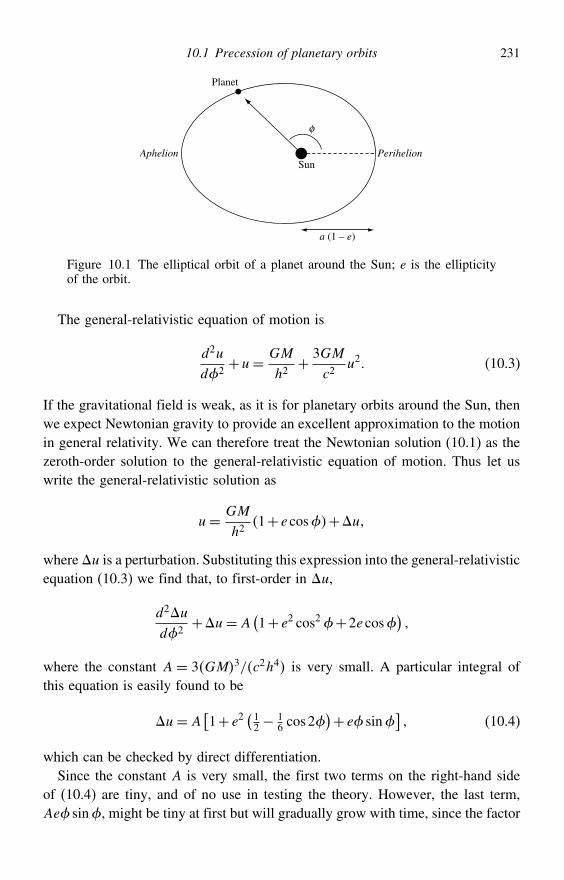
10.1 Precession of planetary orbits 231
Planet
φ
SunPerihelionAphelion
a (1 – e)
Figure 10.1 The elliptical orbit of a planet around the Sun; e is the ellipticityof the orbit.
The general-relativistic equation of motion is
d2u
d2+u= GM
h2+ 3GM
c2u2 (10.3)
If the gravitational field is weak, as it is for planetary orbits around the Sun, thenwe expect Newtonian gravity to provide an excellent approximation to the motionin general relativity. We can therefore treat the Newtonian solution (10.1) as thezeroth-order solution to the general-relativistic equation of motion. Thus let uswrite the general-relativistic solution as
u= GM
h21+ e cos+u
where u is a perturbation. Substituting this expression into the general-relativisticequation (10.3) we find that, to first-order in u,
d2u
d2+u= A
(1+ e2 cos2+2e cos
)
where the constant A = 3GM3/c2h4 is very small. A particular integral ofthis equation is easily found to be
u= A[1+ e2
( 12 − 1
6 cos 2)+ e sin
] (10.4)
which can be checked by direct differentiation.Since the constant A is very small, the first two terms on the right-hand side
of (10.4) are tiny, and of no use in testing the theory. However, the last term,Ae sin, might be tiny at first but will gradually grow with time, since the factor
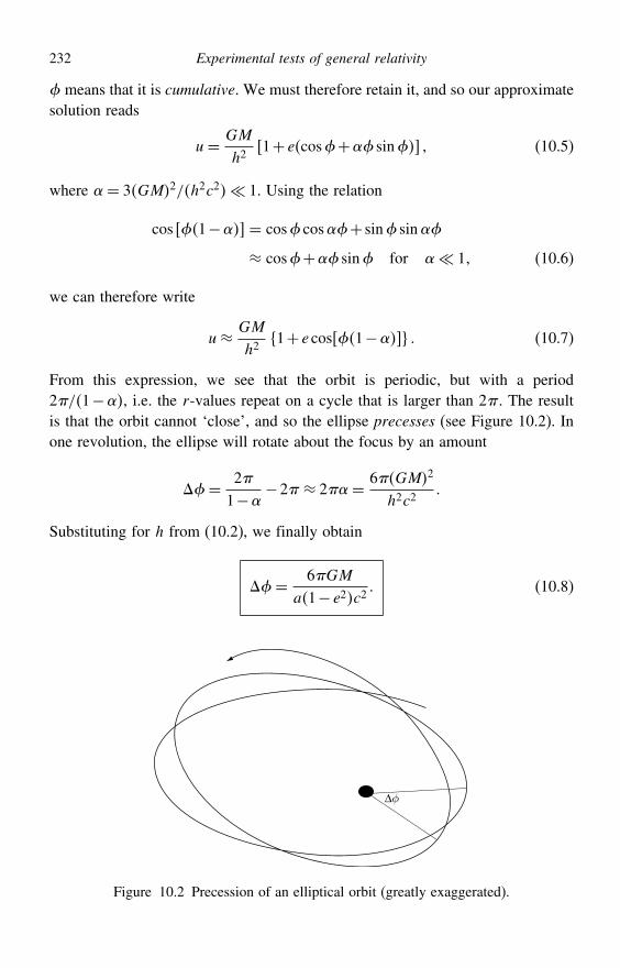
232 Experimental tests of general relativity
means that it is cumulative. We must therefore retain it, and so our approximatesolution reads
u= GM
h2 1+ ecos+ sin (10.5)
where = 3GM2/h2c2 1. Using the relation
cos 1− = cos cos+ sin sin
≈ cos+ sin for 1 (10.6)
we can therefore write
u≈ GM
h2!1+ e cos 1−" (10.7)
From this expression, we see that the orbit is periodic, but with a period2/1−, i.e. the r-values repeat on a cycle that is larger than 2. The resultis that the orbit cannot ‘close’, and so the ellipse precesses (see Figure 10.2). Inone revolution, the ellipse will rotate about the focus by an amount
= 21−
−2 ≈ 2= 6GM2
h2c2
Substituting for h from (10.2), we finally obtain
= 6GM
a1− e2c2 (10.8)
∆φ
Figure 10.2 Precession of an elliptical orbit (greatly exaggerated).
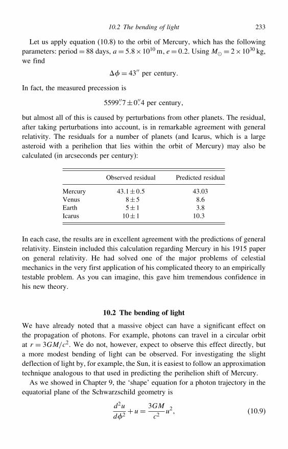
10.2 The bending of light 233
Let us apply equation (10.8) to the orbit of Mercury, which has the followingparameters: period= 88 days, a= 58×1010 m e= 02. UsingM = 2×1030 kg,we find
= 43′′ per century
In fact, the measured precession is
5599′′7±0′′4 per century
but almost all of this is caused by perturbations from other planets. The residual,after taking perturbations into account, is in remarkable agreement with generalrelativity. The residuals for a number of planets (and Icarus, which is a largeasteroid with a perihelion that lies within the orbit of Mercury) may also becalculated (in arcseconds per century):
Observed residual Predicted residual
Mercury 431±05 43.03Venus 8±5 8.6Earth 5±1 3.8Icarus 10±1 10.3
In each case, the results are in excellent agreement with the predictions of generalrelativity. Einstein included this calculation regarding Mercury in his 1915 paperon general relativity. He had solved one of the major problems of celestialmechanics in the very first application of his complicated theory to an empiricallytestable problem. As you can imagine, this gave him tremendous confidence inhis new theory.
10.2 The bending of light
We have already noted that a massive object can have a significant effect onthe propagation of photons. For example, photons can travel in a circular orbitat r = 3GM/c2. We do not, however, expect to observe this effect directly, buta more modest bending of light can be observed. For investigating the slightdeflection of light by, for example, the Sun, it is easiest to follow an approximationtechnique analogous to that used in predicting the perihelion shift of Mercury.
As we showed in Chapter 9, the ‘shape’ equation for a photon trajectory in theequatorial plane of the Schwarzschild geometry is
d2u
d2+u= 3GM
c2u2 (10.9)
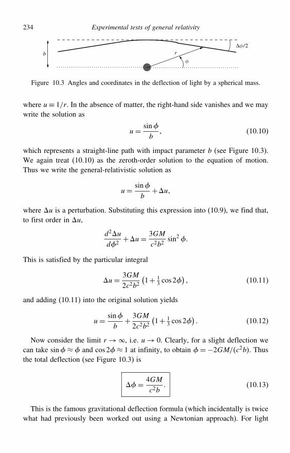
234 Experimental tests of general relativity
b r
φ
∆φ /2
Figure 10.3 Angles and coordinates in the deflection of light by a spherical mass.
where u≡ 1/r . In the absence of matter, the right-hand side vanishes and we maywrite the solution as
u= sinb
(10.10)
which represents a straight-line path with impact parameter b (see Figure 10.3).We again treat (10.10) as the zeroth-order solution to the equation of motion.Thus we write the general-relativistic solution as
u= sinb
+u
where u is a perturbation. Substituting this expression into (10.9), we find that,to first order in u,
d2u
d2+u= 3GM
c2b2sin2
This is satisfied by the particular integral
u= 3GM
2c2b2(1+ 1
3 cos 2) (10.11)
and adding (10.11) into the original solution yields
u= sinb
+ 3GM
2c2b2(1+ 1
3 cos 2) (10.12)
Now consider the limit r→, i.e. u→ 0. Clearly, for a slight deflection wecan take sin≈ and cos2≈ 1 at infinity, to obtain =−2GM/c2b. Thusthe total deflection (see Figure 10.3) is
= 4GM
c2b (10.13)
This is the famous gravitational deflection formula (which incidentally is twicewhat had previously been worked out using a Newtonian approach). For light
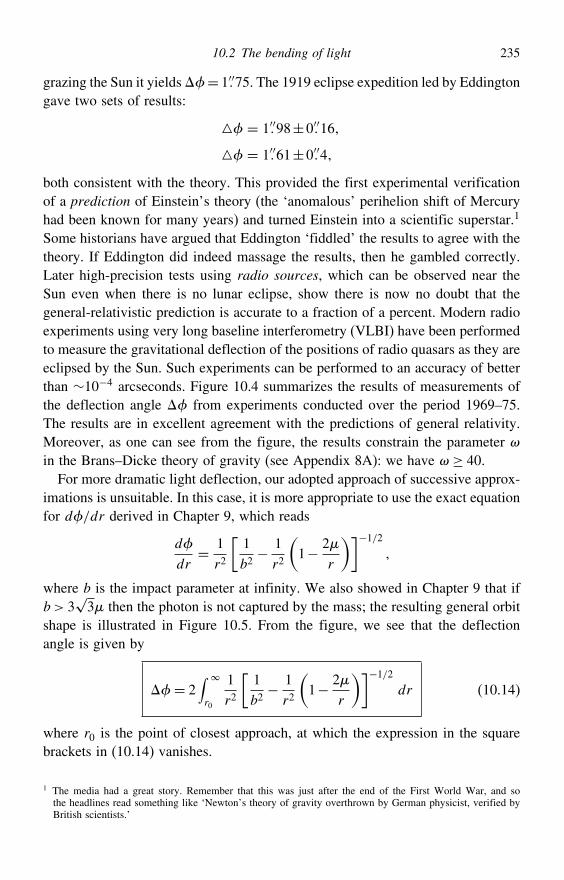
10.2 The bending of light 235
grazing the Sun it yields= 1′′75. The 1919 eclipse expedition led by Eddingtongave two sets of results:
= 1′′98±0′′16
= 1′′61±0′′4
both consistent with the theory. This provided the first experimental verificationof a prediction of Einstein’s theory (the ‘anomalous’ perihelion shift of Mercuryhad been known for many years) and turned Einstein into a scientific superstar.1
Some historians have argued that Eddington ‘fiddled’ the results to agree with thetheory. If Eddington did indeed massage the results, then he gambled correctly.Later high-precision tests using radio sources, which can be observed near theSun even when there is no lunar eclipse, show there is now no doubt that thegeneral-relativistic prediction is accurate to a fraction of a percent. Modern radioexperiments using very long baseline interferometry (VLBI) have been performedto measure the gravitational deflection of the positions of radio quasars as they areeclipsed by the Sun. Such experiments can be performed to an accuracy of betterthan ∼10−4 arcseconds. Figure 10.4 summarizes the results of measurements ofthe deflection angle from experiments conducted over the period 1969–75.The results are in excellent agreement with the predictions of general relativity.Moreover, as one can see from the figure, the results constrain the parameter in the Brans–Dicke theory of gravity (see Appendix 8A): we have ≥ 40.For more dramatic light deflection, our adopted approach of successive approx-
imations is unsuitable. In this case, it is more appropriate to use the exact equationfor d/dr derived in Chapter 9, which reads
d
dr= 1
r2
[1b2− 1r2
(1− 2
r
)]−1/2
where b is the impact parameter at infinity. We also showed in Chapter 9 that ifb > 3
√3 then the photon is not captured by the mass; the resulting general orbit
shape is illustrated in Figure 10.5. From the figure, we see that the deflectionangle is given by
= 2∫
r0
1r2
[1b2− 1r2
(1− 2
r
)]−1/2dr (10.14)
where r0 is the point of closest approach, at which the expression in the squarebrackets in (10.14) vanishes.
1 The media had a great story. Remember that this was just after the end of the First World War, and sothe headlines read something like ‘Newton’s theory of gravity overthrown by German physicist, verified byBritish scientists.’
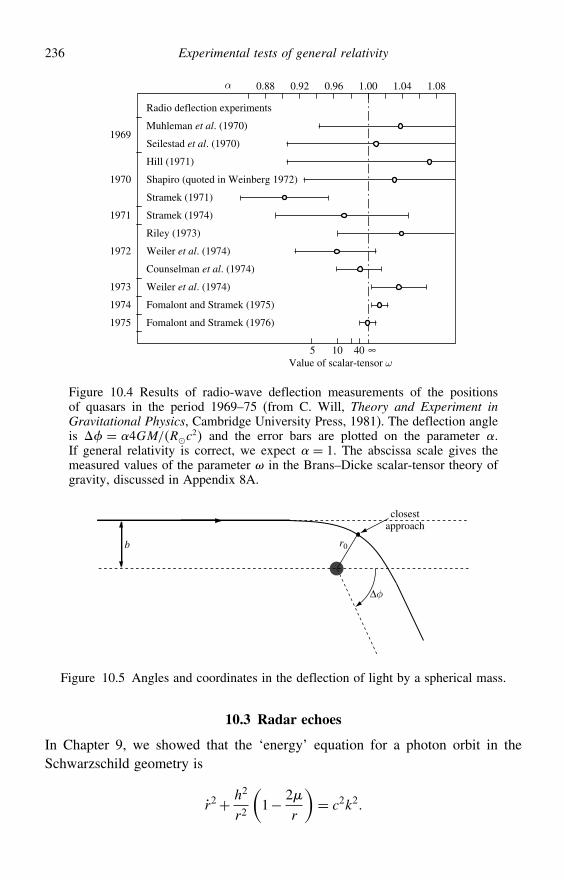
236 Experimental tests of general relativity
Weiler et al. (1974)
Counselman et al. (1974)
Weiler et al. (1974)
Fomalont and Stramek (1975)
Fomalont and Stramek (1976)
Riley (1973)
Stramek (1974)
Stramek (1971)
Shapiro (quoted in Weinberg 1972)
Hill (1971)
Seilestad et al. (1970)
Muhleman et al. (1970)
Radio deflection experiments
1969
1970
1971
1972
1973
1974
1975
α 0.88 1.081.041.000.960.92
5 10 40Value of scalar-tensor ω
∞
Figure 10.4 Results of radio-wave deflection measurements of the positionsof quasars in the period 1969–75 (from C. Will, Theory and Experiment inGravitational Physics, Cambridge University Press, 1981). The deflection angleis = 4GM/Rc2 and the error bars are plotted on the parameter .If general relativity is correct, we expect = 1. The abscissa scale gives themeasured values of the parameter in the Brans–Dicke scalar-tensor theory ofgravity, discussed in Appendix 8A.
b
closestapproach
r0
∆φ
Figure 10.5 Angles and coordinates in the deflection of light by a spherical mass.
10.3 Radar echoes
In Chapter 9, we showed that the ‘energy’ equation for a photon orbit in theSchwarzschild geometry is
r2+ h2
r2
(1− 2
r
)= c2k2
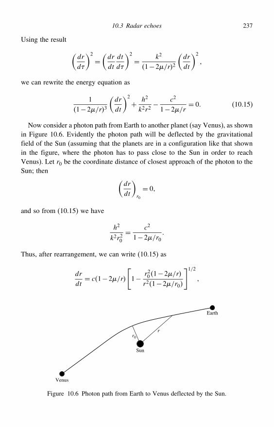
10.3 Radar echoes 237
Using the result (dr
d
)2
=(dr
dt
dt
d
)2
= k2
1−2/r2
(dr
dt
)2
we can rewrite the energy equation as
11−2/r3
(dr
dt
)2
+ h2
k2r2− c2
1−2/r= 0 (10.15)
Now consider a photon path from Earth to another planet (say Venus), as shownin Figure 10.6. Evidently the photon path will be deflected by the gravitationalfield of the Sun (assuming that the planets are in a configuration like that shownin the figure, where the photon has to pass close to the Sun in order to reachVenus). Let r0 be the coordinate distance of closest approach of the photon to theSun; then (
dr
dt
)r0
= 0
and so from (10.15) we have
h2
k2r20= c2
1−2/r0
Thus, after rearrangement, we can write (10.15) as
dr
dt= c1−2/r
[1− r20 1−2/r
r21−2/r0
]1/2
Sun
r0
r
Earth
Venus
Figure 10.6 Photon path from Earth to Venus deflected by the Sun.
238 Experimental tests of general relativity
which can be integrated to give for the time taken to travel between points r0and r
tr r0=∫ r
r0
1c1−2/r
[1− r20 1−2/r
r21−2/r0
]−1/2dr
The integrand can be expanded to first order in /r to obtain
tr r0=∫ r
r0
r
cr2− r20
[1+ 2
r+ r0rr+ r0
]dr
which can be evaluated to give
tr r0=r2− r20
1/2
c+ 2
cln
[r+ r2− r20
1/2
r0
]+
c
(r− r0r+ r0
)1/2
(10.16)
The first term on the right-hand side is just what we would have expected ifthe light had been travelling in a straight line. The second and third terms give usthe extra coordinate time taken for the photon to travel along the curved path tothe point r . So, you can see from Figure 10.6 that if we bounce a radar beam toVenus and back then the excess coordinate-time delay over a straight-line path is
t = 2
[trE r0+ trV r0−
(r2E− r20
)1/2c
−(r2V− r20
)1/2c
]
where the factor 2 is included because the photon has to go to Venus and back.Since rE r0 and rV r0 we have
trE r0−(r2E− r20
)1/2c
≈ 2c
ln(rEr0
)+
c
and likewise for tV and rV. Thus, the excess coordinate-time delay is
t ≈ 4GM
c3
[ln
(rErV
r20
)+1
]
Of course, clocks on earth do not measure coordinate time but the correspondingproper time. Assuming the Earth to be at fixed coordinates r during thetravel time of the signal, this is given by
=(1− 2GM
c2rE
)1/2
t
However, since rE GM/c2, we can ignore this effect to the accuracy of ourcalculation. For Venus, when it is opposite to the Earth on the far side of the Sun,
≈ 220's
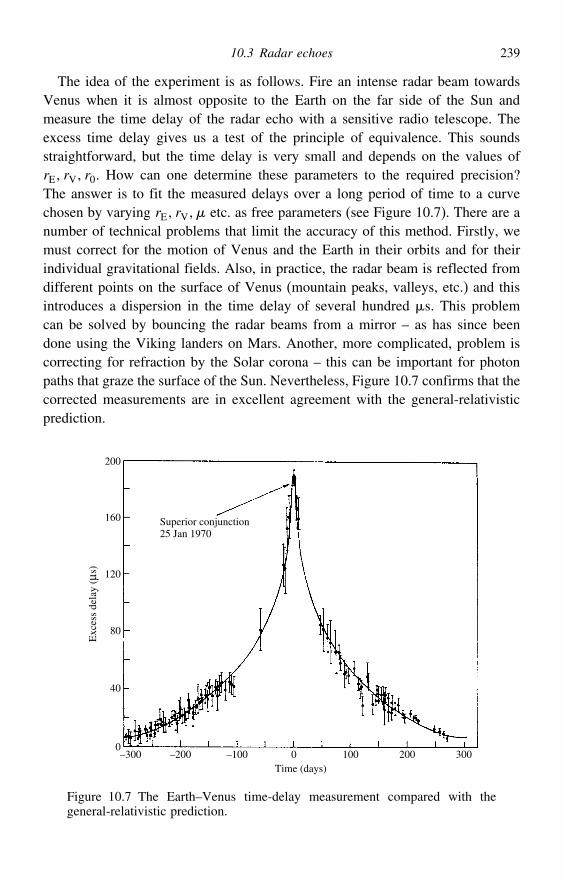
10.3 Radar echoes 239
The idea of the experiment is as follows. Fire an intense radar beam towardsVenus when it is almost opposite to the Earth on the far side of the Sun andmeasure the time delay of the radar echo with a sensitive radio telescope. Theexcess time delay gives us a test of the principle of equivalence. This soundsstraightforward, but the time delay is very small and depends on the values ofrE rV r0. How can one determine these parameters to the required precision?The answer is to fit the measured delays over a long period of time to a curvechosen by varying rE rV etc. as free parameters (see Figure 10.7). There are anumber of technical problems that limit the accuracy of this method. Firstly, wemust correct for the motion of Venus and the Earth in their orbits and for theirindividual gravitational fields. Also, in practice, the radar beam is reflected fromdifferent points on the surface of Venus (mountain peaks, valleys, etc.) and thisintroduces a dispersion in the time delay of several hundred 's. This problemcan be solved by bouncing the radar beams from a mirror – as has since beendone using the Viking landers on Mars. Another, more complicated, problem iscorrecting for refraction by the Solar corona – this can be important for photonpaths that graze the surface of the Sun. Nevertheless, Figure 10.7 confirms that thecorrected measurements are in excellent agreement with the general-relativisticprediction.
–300 –200 –100 0 200 300100Time (days)
Superior conjunction25 Jan 1970
200
160
120
80
40
0
Exc
ess
dela
y (µ
s)
Figure 10.7 The Earth–Venus time-delay measurement compared with thegeneral-relativistic prediction.
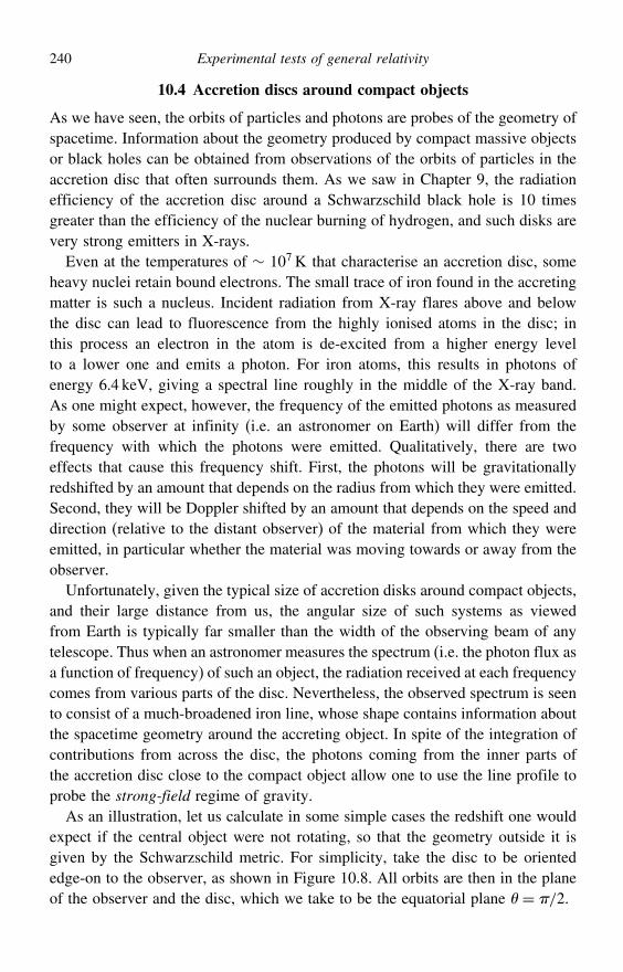
240 Experimental tests of general relativity
10.4 Accretion discs around compact objects
As we have seen, the orbits of particles and photons are probes of the geometry ofspacetime. Information about the geometry produced by compact massive objectsor black holes can be obtained from observations of the orbits of particles in theaccretion disc that often surrounds them. As we saw in Chapter 9, the radiationefficiency of the accretion disc around a Schwarzschild black hole is 10 timesgreater than the efficiency of the nuclear burning of hydrogen, and such disks arevery strong emitters in X-rays.
Even at the temperatures of ∼ 107 K that characterise an accretion disc, someheavy nuclei retain bound electrons. The small trace of iron found in the accretingmatter is such a nucleus. Incident radiation from X-ray flares above and belowthe disc can lead to fluorescence from the highly ionised atoms in the disc; inthis process an electron in the atom is de-excited from a higher energy levelto a lower one and emits a photon. For iron atoms, this results in photons ofenergy 6.4 keV, giving a spectral line roughly in the middle of the X-ray band.As one might expect, however, the frequency of the emitted photons as measuredby some observer at infinity (i.e. an astronomer on Earth) will differ from thefrequency with which the photons were emitted. Qualitatively, there are twoeffects that cause this frequency shift. First, the photons will be gravitationallyredshifted by an amount that depends on the radius from which they were emitted.Second, they will be Doppler shifted by an amount that depends on the speed anddirection (relative to the distant observer) of the material from which they wereemitted, in particular whether the material was moving towards or away from theobserver.
Unfortunately, given the typical size of accretion disks around compact objects,and their large distance from us, the angular size of such systems as viewedfrom Earth is typically far smaller than the width of the observing beam of anytelescope. Thus when an astronomer measures the spectrum (i.e. the photon flux asa function of frequency) of such an object, the radiation received at each frequencycomes from various parts of the disc. Nevertheless, the observed spectrum is seento consist of a much-broadened iron line, whose shape contains information aboutthe spacetime geometry around the accreting object. In spite of the integration ofcontributions from across the disc, the photons coming from the inner parts ofthe accretion disc close to the compact object allow one to use the line profile toprobe the strong-field regime of gravity.
As an illustration, let us calculate in some simple cases the redshift one wouldexpect if the central object were not rotating, so that the geometry outside it isgiven by the Schwarzschild metric. For simplicity, take the disc to be orientededge-on to the observer, as shown in Figure 10.8. All orbits are then in the planeof the observer and the disc, which we take to be the equatorial plane = /2.
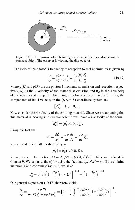
10.4 Accretion discs around compact objects 241
Photon path
Observer
uE
p(E)
r φ
Figure 10.8 The emission of a photon by matter in an accretion disc around acompact object. The observer is viewing the disc edge-on.
The ratio of the photon’s frequency at reception to that at emission is given by
RE= pR ·uR
pE ·uE= pRu
R
pEuE
(10.17)
where pE and pR are the photon 4-momenta at emission and reception respec-tively, uE is the 4-velocity of the material at emission and uR is the 4-velocityof the observer at reception. Assuming the observer to be fixed at infinity, thecomponents of his 4-velocity in the t r coordinate system are[
uR
]= 1000
Now consider the 4-velocity of the emitting material. Since we are assuming thatthis material is moving in a circular orbit it must have a 4-velocity of the form[
uE
]= (u0E00 u3E) Using the fact that
u3E =d
d= d
dt
dt
d= d
dtu0E
we can write the emitter’s 4-velocity as
uE= u0E100
where, for circular motion, ≡ d/dt = GM/r31/2, which we derived inChapter 9. We can now fix u0E by using the fact that gu
u = c2. If the emittingmaterial is at a coordinate radius r, we have
u0E = c
[c2(1− 2
r
)− r22
]−1/2=(1− 3
r
)−1/2
Our general expression (10.17) therefore yields
RE= p0R
p0Eu0E+p3Eu
3E
=(1− 3
r
)1/2 p0R
p0E
[1± p3E
p0E
]−1
242 Experimental tests of general relativity
where the plus sign corresponds to the emitting matter on the side of the discmoving towards the observer and the minus sign corresponds to the matter onthe other side. However, the Schwarzschild metric is stationary, i.e. the metriccomponents g do not depend explicitly on t. Thus p0 is conserved along thegeodesic, and so
RE=(1− 3
r
)1/2 [1± p3E
p0E
]−1
It therefore remains only to fix the ratio p3E/p0E in order to determine theobserved redshift. In general, we must use the fact that the photon worldline isnull, and so gpp = 0. As we are working in the equatorial plane = /2,this yields
1c2
(1− 2
r
)−1p0
2−(1− 2
r
)p1
2− 1r2p3
2 = 0 (10.18)
For photons emitted from material at a general position angle , one would nowneed to use the geodesic equations for the photon worldline in order to eliminatep1. There are, however, two special cases for which this is not necessary.
The simplest case occurs when the photon is emitted from matter movingtransverse to the observer, i.e. when = 0 or = . We then have p3E = 0,and so the observed frequency ratio is
RE=(1− 3
r
)1/2
(10.19)
The other simple cases occur when the matter is moving either directly towardsor away from the observer, i.e. when = −/2 or = /2. Then the radialcomponents of the photon 4-momentum, p1E, will be zero. From (10.18) weobtain
p3E
p0E= r
c1−2/r1/2
so that the photon frequency shift for =∓/2 is given by
RE= 1−3/r1/2
1± r/−2−1/2 (10.20)
The above discussion has been for a disc viewed edge-on. The other limiting case,when the disc is viewed face-on, is easier to analyse. Since the motion of theemitting matter is always transverse to the observer, the frequency shift is givenby (10.19).
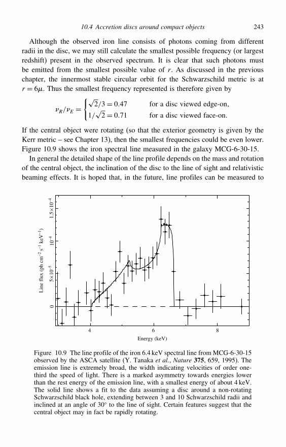
10.4 Accretion discs around compact objects 243
Although the observed iron line consists of photons coming from differentradii in the disc, we may still calculate the smallest possible frequency (or largestredshift) present in the observed spectrum. It is clear that such photons mustbe emitted from the smallest possible value of r. As discussed in the previouschapter, the innermost stable circular orbit for the Schwarzschild metric is atr = 6. Thus the smallest frequency represented is therefore given by
R/E =√
2/3= 047 for a disc viewed edge-on
1/√2= 071 for a disc viewed face-on
If the central object were rotating (so that the exterior geometry is given by theKerr metric – see Chapter 13), then the smallest frequencies could be even lower.Figure 10.9 shows the iron spectral line measured in the galaxy MCG-6-30-15.
In general the detailed shape of the line profile depends on the mass and rotationof the central object, the inclination of the disc to the line of sight and relativisticbeaming effects. It is hoped that, in the future, line profiles can be measured to
4 6 8
Energy (keV)
Lin
e fl
ux (
ph c
m–2
s–1
keV
–1)
010
–41.
5×1
0–45
×10–5
Figure 10.9 The line profile of the iron 6.4 keV spectral line from MCG-6-30-15observed by the ASCA satellite (Y. Tanaka et al., Nature 375, 659, 1995). Theemission line is extremely broad, the width indicating velocities of order one-third the speed of light. There is a marked asymmetry towards energies lowerthan the rest energy of the emission line, with a smallest energy of about 4 keV.The solid line shows a fit to the data assuming a disc around a non-rotatingSchwarzschild black hole, extending between 3 and 10 Schwarzschild radii andinclined at an angle of 30 to the line of sight. Certain features suggest that thecentral object may in fact be rapidly rotating.
244 Experimental tests of general relativity
sufficient accuracy to determine the mass and angular momentum of the centralcompact object.
10.5 The geodesic precession of gyroscopes
We have seen how the motion of test bodies can be used to explore the geometryof a curved spacetime. If the test body has spin then the motion of its spin vectorcan also be used to probe the spacetime geometry. Here we discuss the idealisedcase of an infinitesimally small test body with spin, such as a small gyroscope.
The test body moves along a timelike geodesic curve, so its 4-velocity uis parallel-transported along its worldline. Thus, in some coordinate system, itscomponents satisfy
du
d+
#uu# = 0
Suppose that the spin of the test body is described by the 4-vector s along thegeodesic. Since this vector can have no timelike component in the instantaneousrest frame of the test body, we require that at all points along the geodesic
s ·u= gsu = 0 (10.21)
Since the 4-velocity u of the test body is parallel-transported along its geodesic,to ensure that the inner product is conserved at all points along the worldlinewe require that s is also parallel-transported along the geodesic. Hence itscomponents must satisfy
ds
d+
#su# = 0 (10.22)
Let us now suppose that the test body is in a circular orbit of coordinate radiusr in the equatorial plane of the Schwarzschild geometry. Using the expressions wederived in Chapter 9 for the connection coefficients
# for the Schwarzschildmetric in t r coordinates (with = /2), one finds that most of the
#
are zero. Moreover, for a test body in a circular orbit we have u1 = u2 = 0, andwe find that the equations (10.22) reduce to
ds0
d+ 0
10s1u0 = 0 (10.23)
ds1
d+ 1
00s0u0+ 1
33s3u3 = 0 (10.24)
ds2
d= 0 (10.25)
ds3
d+ 3
13s1u3 = 0 (10.26)
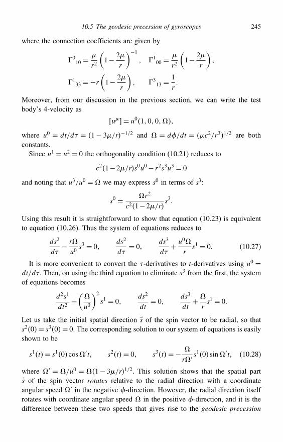
10.5 The geodesic precession of gyroscopes 245
where the connection coefficients are given by
010 =
r2
(1− 2
r
)−1 1
00 =
r2
(1− 2
r
)
133 =−r
(1− 2
r
) 3
13 =1r
Moreover, from our discussion in the previous section, we can write the testbody’s 4-velocity as
u= u0100
where u0 = dt/d = 1− 3/r−1/2 and = d/dt = c2/r31/2 are bothconstants.
Since u1 = u2 = 0 the orthogonality condition (10.21) reduces to
c21−2/rs0u0− r2s3u3 = 0
and noting that u3/u0 = we may express s0 in terms of s3:
s0 = r2
c21−2/rs3
Using this result it is straightforward to show that equation (10.23) is equivalentto equation (10.26). Thus the system of equations reduces to
ds2
d− r
u0s3 = 0
ds2
d= 0
ds3
d+ u0
rs1 = 0 (10.27)
It is more convenient to convert the -derivatives to t-derivatives using u0 =dt/d. Then, on using the third equation to eliminate s3 from the first, the systemof equations becomes
d2s1
dt2+(
u0
)2
s1 = 0ds2
dt= 0
ds3
dt+
rs1 = 0
Let us take the initial spatial direction s of the spin vector to be radial, so thats20= s30= 0. The corresponding solution to our system of equations is easilyshown to be
s1t= s10 cos′t s2t= 0 s3t=−
r′ s10 sin′t (10.28)
where ′ = /u0 = 1− 3/r1/2. This solution shows that the spatial parts of the spin vector rotates relative to the radial direction with a coordinateangular speed ′ in the negative -direction. However, the radial direction itselfrotates with coordinate angular speed in the positive -direction, and it is thedifference between these two speeds that gives rise to the geodesic precession
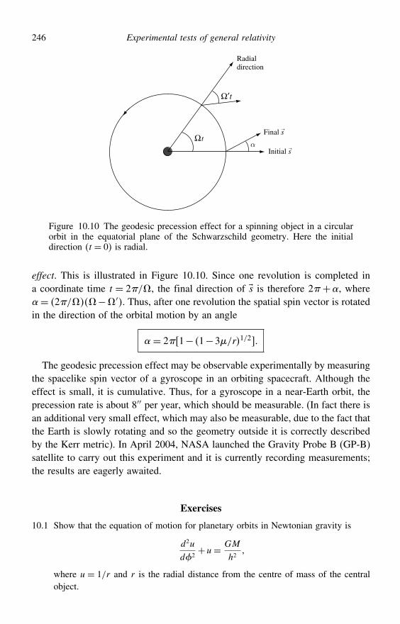
246 Experimental tests of general relativity
Radialdirection
Initial s
Final s
α
Ω′t
Ω t
→
→
Figure 10.10 The geodesic precession effect for a spinning object in a circularorbit in the equatorial plane of the Schwarzschild geometry. Here the initialdirection t = 0 is radial.
effect. This is illustrated in Figure 10.10. Since one revolution is completed ina coordinate time t = 2/, the final direction of s is therefore 2+, where= 2/−′. Thus, after one revolution the spatial spin vector is rotatedin the direction of the orbital motion by an angle
= 2 1− 1−3/r1/2
The geodesic precession effect may be observable experimentally by measuringthe spacelike spin vector of a gyroscope in an orbiting spacecraft. Although theeffect is small, it is cumulative. Thus, for a gyroscope in a near-Earth orbit, theprecession rate is about 8′′ per year, which should be measurable. (In fact there isan additional very small effect, which may also be measurable, due to the fact thatthe Earth is slowly rotating and so the geometry outside it is correctly describedby the Kerr metric). In April 2004, NASA launched the Gravity Probe B (GP-B)satellite to carry out this experiment and it is currently recording measurements;the results are eagerly awaited.
Exercises
10.1 Show that the equation of motion for planetary orbits in Newtonian gravity is
d2u
d2+u= GM
h2
where u = 1/r and r is the radial distance from the centre of mass of the centralobject.
Exercises 247
10.2 Show that the equation of motion in Exercise 10.1 has the solution
u= GM
h21+ e cos
and that this describes an ellipse. Show further that
a= h2
GM1− e2
where r1 = a1− e and r2 = a1+ e are the distances of closest and furthestapproach respectively.
10.3 Verify that the general-relativistic equation of motion for planetary orbits (10.3)has the solution
u= GM
h21+ e cos+ 3GM2
c2h4
[1+ e2
(12− 1
6cos2
)+ e sin
]
to first order in the relativistic perturbation to the Newtonian solution.10.4 Verify that the general-relativistic equation of motion for a photon trajectory (10.9)
has the solution
u= sinb
+ 3GM
2c2b2
(1+ 1
3cos2
)
to first order in the relativistic perturbation to a straight-line path.10.5 Show that the gravitational deflection of light by the Sun predicted in the Newto-
nian theory of gravity is exactly half the value predicted in general relativity.10.6 In the radar-echoes test, a photon travels from radial coordinate r to r0, which is
the radial coordinate of the closest approach of the photon to the Sun. Verify that,to first order in /r, the elapsed coordinate time is given by
tr r0=r2− r20
1/2
c+ 2
cln[r+ r2− r20
1/2
r0
]+
c
(r− r0r+ r0
)1/2
10.7 An accretion disc extends from r = 6 to r = 20 in the equatorial plane of theSchwarzschild geometry. A photon is emitted radially outwards by a particle onthe inner edge of the disc and is absorbed by a particle on the outer edge of thedisc. Find the ratio of the energy absorbed to that emitted.
10.8 For a gyroscope in a circular orbit in the equatorial plane of the Schwarzschildgeometry, show that the components s of its spin 4-vector satisfy equa-tions (10.23–10.26).
10.9 Show that the system of equations (10.27) has the solution (10.28).10.10 A gyroscope in a circular orbit of radius r in the equatorial plane of the
Schwarzschild geometry has its spatial spin vector s also lying in the equatorialplane. Show that, after one complete orbit, the angle between the initial and finaldirections of the spatial spin vector is given by
= 2[1− 1−3/r1/2
]
irrespective of the initial direction of the spin vector. Does this still hold if theoriginal spatial spin vector does not lie in the plane of the orbit?
11
Schwarzschild black holes
In our discussion of the Schwarzschild geometry, we have thus far used thecoordinates t r to label events in the spacetime. In this context, t r are called the Schwarzschild coordinates. Moreover, until now we have beenconcerned only with the exterior region r > 2. We now turn to the discussionof the Schwarzschild geometry in the interior region r < 2, and the significanceof the hypersurface r = 2. We shall see that, in order to understand the entireSchwarzschild geometry, we must relabel the events in spacetime using differentsets of coordinates.
11.1 The characterisation of coordinates
Before discussing the Schwarzschild geometry in detail, let us briefly consider thecharacterisation of coordinates. In general, if we wish to write down a solutionof Einstein’s field equations then we need to do so in some particular coordinatesystem. But what, if any, is the significance of any such system? For example,suppose we take the Schwarzschild solution and apply some complicated coor-dinate transformation x → x′. The resulting metric will still be a solution ofthe empty-space field equations, of course, but there is likely to be little or nophysical or geometrical significance attached to the new coordinates x′.One thing we can do, however, is to establish whether at some event P a
coordinate x is timelike, null or spacelike. This corresponds directly to the natureof the tangent vector e to the coordinate curve at P. The easiest way to determinethis property of the coordinate is to fix the other coordinates at their values at Pand consider an infinitesimal variation dx in the coordinate of interest. If thecorresponding change in the interval ds2 is positive, zero or negative then x istimelike, null or spacelike respectively. This, in turn, corresponds simply to thesign of the relevant diagonal element g (no sum) of the metric.
248
11.2 Singularities in the Schwarzschild metric 249
11.2 Singularities in the Schwarzschild metric
With these ideas in mind, let us look at the Schwarzschild metric in the traditionalt r coordinate system. We have
ds2= c2(1− 2GM
c2r
)dt2−
(1− 2GM
c2r
)−1dr2−r2 d2−r2 sin2 d2 (11.1)
Inspection of this line element shows immediately that the metric is singular atr = 0 and r = 2GM/c2. The latter value is known as the Schwarzschild radiusand is often denoted rS, so that
rS =2GM
c2
We must remember, however, that we derived the Schwarzschild solution bysolving the vacuum field equations R = 0, and so the metric given by (11.1) isonly valid down to the surface of the spherical matter distribution. For example,the Schwarzschild radius for the Sun is
rS =2GMc2
= 295km
which is much smaller than the radius of the Sun R = 7×10⁵ km. Similarly,the Schwarzschild radius for a proton is
rS =2GMp
c2= 10−52 m
again much smaller than the characteristic radius of a proton (Rp = 10−15 m). Infact, for most real objects the Schwarzschild radius lies deep within the object,where the vacuum field equations do not apply. But what if there exist objects socompact that they lie well within the Schwarzschild radius? For such an object, theSchwarzschild solution looks very odd. Ignoring for the moment the singularityin the metric at r = rS, let us denote the region r > rS as region I, and r < rS asregion II.
From the Schwarzschild metric (11.1) we see that, in region I, the metriccoefficient g00 is positive and the gii (for i = 123) are negative. It thereforefollows that for r > rS the coordinate t is timelike and the coordinates r
are spacelike. Indeed, in region I we may attach simple physical meanings to thecoordinates. For example, t is the proper time measured by an observer at rest atinfinity. Similarly, r is a radial coordinate with the property that the surface areaof a 2-sphere t= constant, r = constant is 4r2. In region II, however, the metric
250 Schwarzschild black holes
coefficients g00 and g11 change sign. Hence, for r < rS , t is a spacelike coordinateand r is timelike. Thus ‘time’ and ‘radial’ coordinates swap character on eitherside of r = rS. It is natural to ask what this means, and, indeed, whether it isphysically meaningful.
Let us therefore consider in more detail the singularities in the metric atr = 0 and r = rS. We must remember that coordinates are simply a way oflabelling events in spacetime. The physically meaningful geometric quantites arethe 4-tensors defined at any point on the spacetime manifold. Spacetime curvatureis described covariantly by the components of the curvature tensor R# (and itscontractions), which we may easily calculate for the Schwarzschild metric (11.1).For example, the curvature scalar at any point is given by
R#R# = 482
r6 (11.2)
which we see is finite at r = rS. Moreover, since it is a scalar, its value remainsthe same in all coordinate systems. Thus the spacetime curvature at r = rS isperfectly well behaved, and so we see that r = rS is a coordinate singularity. Bythe same token, (11.2) is singular at r = 0 and so this point is a true intrinsicsingularity of the Schwarzschild geometry.
We may illustrate the idea of coordinate singularities with a simple example.As discussed in Chapter 2, one may write the line element for the surface of a2-sphere as
ds2 = a2d2
a2−2+2 d2
This line element has a singularity at = a. Embedding this manifold, for themoment, in three-dimensional Euclidean space, we know that = a correspondssimply to the equator of the sphere (relative to the origin of the coordinate system)and it is clear why the coordinates cover the surface of the sphere uniquelyonly up to this point. There is nothing pathological occurring in the intrinsic geom-etry of the 2-sphere at the equator, i.e. there is no ‘real’ (or intrinsic) singularityin the metric. As shown in Appendix 7A, the Gaussian curvature of a 2-sphereis simply K = 1/a2, which does not ‘blow up’ anywhere. Thus, = a is only acoordinate singularity, which has resulted simply from choosing coordinates witha restricted domain of validity. In an analogous way, the coordinate singularityof the Schwarzschild metric is simply a result of the coordinate system that wehave chosen to use. We can remove it by making appropriate transformationsof coordinates, which we will discuss later. For the time being, however, let uscontinue our investigation of the Schwarzschild geometry using the Schwarzschildcoordinates t r .
11.3 Radial photon worldlines in Schwarzschild coordinates 251
11.3 Radial photon worldlines in Schwarzschild coordinates
Let us investigate the spacetime diagram of the Schwarzschild solution int r coordinates. The metric reads
ds2 = c2(1− 2
r
)dt2−
(1− 2
r
)−1dr2− r2 d2
where d is an element of solid angle. We have written it in this form becausewe shall usually ignore the angular coordinates in drawing spacetime diagrams,i.e. these diagrams will show the r ct-plane for fixed values of and .
We begin by determining the lightcone structure in the diagram, by consideringthe paths of radially incoming and outgoing photons; these were discussed brieflyin Section 9.11. From the metric, for a radially moving photon we have
dt
dr=±1
c
(1− 2
r
)−1
where the plus sign corresponds to a photon that is outgoing (in that dr/dt ispositive in the region r > 2) and the minus sign corresponds to a photon thatis incoming (in that dr/dt is negative in the region r > 2). On integrating, weobtain
ct = r+2 ln
∣∣∣∣ r2 −1
∣∣∣∣+ constant outgoing photon
ct = −r−2 ln
∣∣∣∣ r2 −1
∣∣∣∣+ constant incoming photon
Notice that under the transformation t→−t the incoming and outgoing photonpaths are interchanged, as we would expect. We can now plot these curves in ther ct-plane, as shown in Figure 11.1. The diagram is drawn for fixed and .Since the diagram will be the same for all other and , we should think of eachpoint r ct in the diagram as representing a 2-sphere of area 4r2.Figure 11.1 requires some words of explanation. At large radii in region I the
gravitational field becomes weak and the metric tends to the Minkowski metricof special relativity. Thus, as expected, the lightcone structure becomes that ofMinkowski spacetime, where incoming and outgoing light rays define straightlines of slope ±1 in the diagram. As we approach the Schwarzschild radius, theingoing light rays tend to the ordinate t→+ and outgoing light rays tend tot→−. This seems to suggest that it takes an infinite time for an incoming signalto cross the Schwarzschild radius, but in this respect the diagram is misleading,as we shall see shortly (we discussed this point briefly in Section 9.11).
252 Schwarzschild black holes
Ingoing nullcongruence
Outgoing nullcongruence
I
Singularity
r = 2µr = 0
ct
II
Figure 11.1 Lightcone structure of the Schwarzschild solution.
In region II the lightcones flip their orientation by 90, since the coordinatest and r reverse their character. We see that all photons in this region must endup at r = 0. At this point there is real singularity, where the curvature of theSchwarzschild solution diverges. Moreover, any massive particle in region IImust also end up at the singularity, since a timelike worldline must lie withinthe forward light-cone at each point. Thus we conclude that once within theSchwarzschild radius you necessarily end up at a spacelike singularity at r = 0.To escape would require a violation of causality.
11.4 Radial particle worldlines in Schwarzschild coordinates
The causal structure in Figure 11.1 is determined by radially moving photons.It is also of interest to determine the worldlines of radially moving massiveparticles in Schwarzschild coordinates. For simplicity let us consider an infallingparticle released from rest at infinity, which we investigated in detail in Chapter 9.Parameterising the particle worldline in terms of the proper time , we found thatthe trajectory r could be written implicitly as
= 23
√r30
2c2− 2
3
√r3
2c2 (11.3)
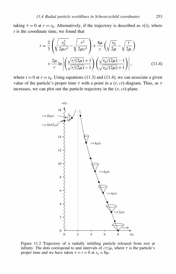
11.4 Radial particle worldlines in Schwarzschild coordinates 253
taking = 0 at r = r0. Alternatively, if the trajectory is described as rt, wheret is the coordinate time, we found that
t = 23
⎛⎝√ r302c2
−√
r3
2c2
⎞⎠+ 4c
(√r02−√
r
2
)
+ 2c
ln
∣∣∣∣∣(√
r/2+1√r/2−1
)(√r0/2−1√r0/2+1
)∣∣∣∣∣ (11.4)
where t= 0 at r = r0. Using equations (11.3) and (11.4), we can associate a givenvalue of the particle’s proper time with a point in a r ct-diagram. Thus, as increases, we can plot out the particle trajectory in the r ct-plane.
r/µ
ct/µ
τ = 10µ /c
τ = 10.67µ /c
2
4
6
8
14
10
12
18
τ = 8µ /c
τ = 6µ /c
τ = 4µ /c
τ = 2µ /c
τ = 0
2 4 6 80
0
Figure 11.2 Trajectory of a radially infalling particle released from rest atinfinity. The dots correspond to unit intervals of c/, where is the particle’sproper time and we have taken = t = 0 at r0 = 8.
254 Schwarzschild black holes
The corresponding curve is shown in Figure 11.2, which is a more quantitativeversion of Figure 9.6; we have taken = t = 0 at r0 = 8. Also plotted are dotsshowing unit intervals of c/, together with the light-cone structure at particularpoints on the trajectory. We see from the plot that the particle worldline has asingularity at r = 2 and that it takes an infinite coordinate time t for the particleto travel from r = 8 to r = 2. Since t is the time experienced by a stationaryobserver at large radius, to such an observer it thus takes an infinite time for theparticle to reach r = 2. However, the proper time taken by the particle to reachr = 2 is finite ( = 933/c). Moreover, we see that for later values of theparticle worldline lies in the region r < 2, which was not plotted in Figure 9.6.In this region the coordinates t and r swap character, as indicated by the factthat the light-cone is flipped by 90. For r < 2, we also note that, although
continues to increase until r = 0 is reached ( = 1067/c), the coordinate timet decreases along the particle worldline.
Clearly, although the coordinate t is useful and physically meaningful as r→,it is inappropriate for describing particle motion at r ≤ 2. Therefore, in thefollowing section we introduce a new time coordinate that is adapted to describingradial infall, and in the process we shall remove the coordinate singularity atr = 2.
11.5 Eddington–Finkelstein coordinates
The spacetime diagrams in Figures 11.1 and 11.2 show that the worldlines ofboth radially moving photons and massive particles cross r = 2 only at t=±.This suggests that the ‘line’ r = 2, −< t < might really not be a line at all,but a single point. That is, our coordinates may go bad owing to the expansionof a single event into the whole line r = 2. One technique for circumventingthe problem of unsatisfactory coordinates is to ‘probe’ spacetime with geodesics,which after all are coordinate independent and will not be affected in any way bythe boundaries of coordinate validity. Of the many possibilities, we will use asprobes the null worldlines of radially moving photons.1
Advanced Eddington–Finkelstein coordinates
Since in particular, we wish, to develop a better description of infalling particles,let us begin by constructing a new coordinate system based on radially infalling
1 It is also possible to use the timelike worldlines of freely falling radially moving massive particles as probes ofthe spacetime geometry. The traditional approach leads to useful new coordinates, called Novikov coordinates,but they are related to Schwarzschild coordinates by transformations that are algebraically very complicated.A more physically meaningful set of new coordinates that are also based on radially moving massive particlegeodesics is discussed in Exercise 11.9.
11.5 Eddington–Finkelstein coordinates 255
photons. Recall that the worldline of a radially ingoing photon is given by
ct =−r−2 ln
∣∣∣∣ r2 −1
∣∣∣∣+ constant
The trick is to use the integration constant as the new coordinate, which wedenote by p. Thus, we make the coordinate transformation
p= ct+ r+2 ln
∣∣∣∣ r2 −1
∣∣∣∣ (11.5)
where p, for historical reasons, is known as the advanced time parameter and isclearly a null coordinate (see Section 11.1). Since p is constant along the entireworldline of the radially ingoing photon, it will be a ‘good’ coordinate whereverthat worldline penetrates.
Differentiating (11.5), we obtain
dp= c dt+ r
r−2dr
and, on substituting for dt in the Schwarzschild line element, we find that interms of the parameter p the line element takes the simple form
ds2 =(1− 2
r
)dp2−2dpdr− r2
(d2+ sin2 d2) (11.6)
We see immediately from (11.6) that ds2 is now regular at r = 2; indeed it isregular for the whole range 0< r <, which is the range of r-values probed byan infalling photon geodesic. Thus, in some sense, the transformation (11.5) hasextended the coordinate range of the solution in a way reminiscent of the analyticcontinuation of a complex function.
One might object that the coordinate transformation (11.5) cannot be used atr = 2 because it becomes singular. This must happen, however, if one is toremove the coordinate singularity there. In any case, this transformation takes thestandard form (11.1) for the Schwarzschild line element to the form (11.6). Giventhese two solutions, we can simply ask, what is the largest range of coordinatesfor which each solution is regular? For the standard form this is 2 < r <,whereas for the new form (11.6) it is 0< r<. In the overlap region 2< r<the two solutions are related by (11.5), and hence they must represent the samesolution in this region.
256 Schwarzschild black holes
As one might expect, the metric (11.6) is especially convenient for calculatingthe paths of null geodesics. In particular, we see that radial null geodesics (forwhich ds = d = d= 0) are given by(
1− 2r
)(dp
dr
)2
−2dp
dr= 0
which has the two solutions
dp
dr= 0 ⇒ p= constant
dp
dr= 2
(1− 2
r
)−1⇒ p= 2r+4 ln
∣∣∣∣ r2 −1
∣∣∣∣+ constant (11.7)
which correspond to incoming and outgoing radial null geodesics respectively(the former being valid by construction).
Since p is a null coordinate, which might be intuitively unfamiliar, it is commonpractice to work instead with the related timelike coordinate t′, defined by
ct′ ≡ p− r = ct+2 ln
∣∣∣∣ r2 −1
∣∣∣∣ (11.8)
The line element then takes the form
ds2 = c2(1− 2
r
)dt′2− 4c
rdt′dr−
(1+ 2
r
)dr2− r2
(d2+ sin2 d2
)
(11.9)
which is again regular for the whole range 0< r<. The coordinates t′ r are called advanced Eddington–Finkelstein coordinates. We note that the lineelement (11.9) is not invariant with respect to the transformation t′ → −t′, underwhich the second term on the right-hand side changes sign. From (11.7), we seethat incoming and outgoing photon worldlines are given by
ct′ = −r+ constant (11.10)
ct′ = r+4 ln
∣∣∣∣ r2 −1
∣∣∣∣+ constant (11.11)
The first equation, for ingoing photons, corresponds to a straight line makingan angle of 45 with the r-axis and is valid for 0 < r < . Thus the photongeodesics are continuous straight lines across r = 2. The spacetime diagram
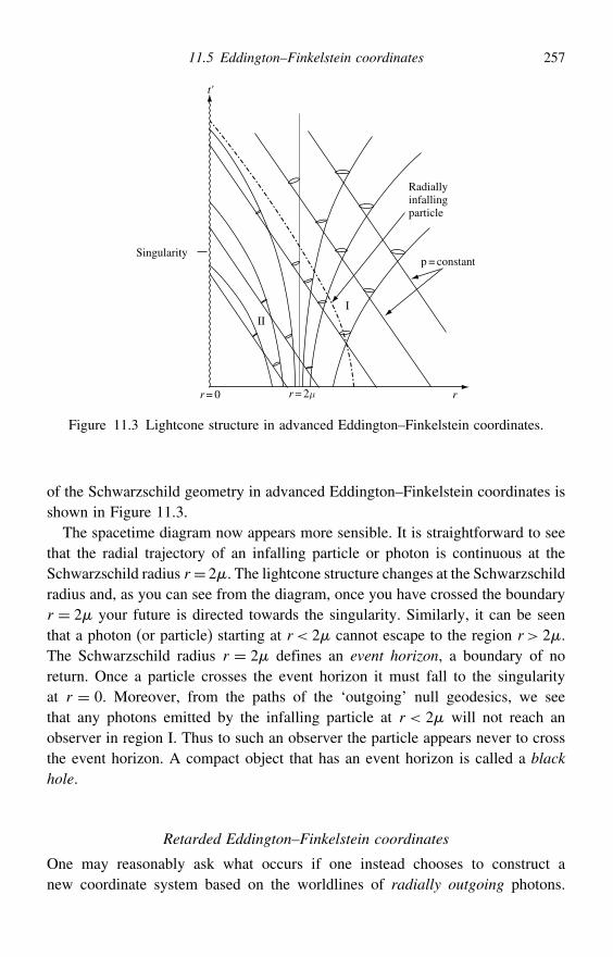
11.5 Eddington–Finkelstein coordinates 257
Radiallyinfallingparticle
r = 2µ
III
Singularity
r = 0
t'
p = constant
r
Figure 11.3 Lightcone structure in advanced Eddington–Finkelstein coordinates.
of the Schwarzschild geometry in advanced Eddington–Finkelstein coordinates isshown in Figure 11.3.
The spacetime diagram now appears more sensible. It is straightforward to seethat the radial trajectory of an infalling particle or photon is continuous at theSchwarzschild radius r = 2. The lightcone structure changes at the Schwarzschildradius and, as you can see from the diagram, once you have crossed the boundaryr = 2 your future is directed towards the singularity. Similarly, it can be seenthat a photon (or particle) starting at r < 2 cannot escape to the region r > 2.The Schwarzschild radius r = 2 defines an event horizon, a boundary of noreturn. Once a particle crosses the event horizon it must fall to the singularityat r = 0. Moreover, from the paths of the ‘outgoing’ null geodesics, we seethat any photons emitted by the infalling particle at r < 2 will not reach anobserver in region I. Thus to such an observer the particle appears never to crossthe event horizon. A compact object that has an event horizon is called a blackhole.
Retarded Eddington–Finkelstein coordinates
One may reasonably ask what occurs if one instead chooses to construct anew coordinate system based on the worldlines of radially outgoing photons.
258 Schwarzschild black holes
By analogy with our discussion above, this is achieved straightforwardly by intro-ducing the new null coordinate q defined by
q = ct− r−2 ln
∣∣∣∣ r2 −1
∣∣∣∣ which is known as the retarded time parameter. The line element of theSchwarzschild geometry then becomes
ds2 =(1− 2
r
)dq2+2dq dr− r2d2+ sin2 d2
which is again regular for 0< r<. Similarly, it is common practice to introducea new timelike coordinate t∗ defined by
ct∗ ≡ q+ r = ct−2 ln
∣∣∣∣ r2 −1
∣∣∣∣ The coordinates t∗ r are called retarded Eddington–Finkelstein coordi-nates, and the corresponding line element in these coordinates is simply the timereversal of the advanced Eddington–Finkelstein line element (11.9).
It is straightforward to draw an spacetime diagram analogous to Figure 11.3 inretarded Eddington–Finkelstein coordinates, and one finds that (by construction)the outgoing radial null geodesics are continuous straight lines at 45 but theingoing null rays are discontinuous, tending to t∗ = + at r = 2. In this case,the surface r = 2 again acts as a one-way membrane, but this time letting onlyoutgoing timelike or null geodesics cross from inside to outside. Indeed, particlesmust move away from the singularity at r = 0 and are forcibly expelled from theregion r < 2. Such an object is called a white hole.
This behaviour appears completely at odds with our intuition regarding thegravitational attraction of a massive body. Moreover, how can the physicalprocesses that occur be so radically different depending on one’s choice of coordi-nates, since we have maintained throughout that coordinates are merely arbitrarylabels of spacetime events? The key to resolving this apparent paradox is torealise that our original coordinates t r covered only a part of the ‘full’Schwarzschild geometry. This topic is discussed fully in Section 11.9, in which weintroduce Kruskal coordinates, which cover the entire geometry and which showthat it possesses both a black-hole and a white-hole singularity. The advancedEddington–Finkelstein coordinates ‘extend’ the solution into the (more familiar)part of the manifold that constitutes a black hole, whereas the retarded Eddington–Finkelstein coordinates extend the solution into a different part of the manifold,corresponding to a white hole. As we will discuss in Section 11.9, the existenceof white holes as a physical reality (as opposed to a mathematical curiosity) is
11.6 Gravitational collapse and black-hole formation 259
rather doubtful. Black holes, however, are likely to occur physically, as we nowgo on to discuss.
11.6 Gravitational collapse and black-hole formation
Our investigation of the properties of a black hole would be largely academicunless there were reasons for believing that they might exist in Nature. Thepossibility of their existence arises from the idea of gravitational collapse.
A star is held up by a mixture of gas and radiation pressure, the relativecontributions depending on its mass. The energy to provide this pressure support isderived from the fusion of light nuclei into heavier ones, predominantly hydrogeninto helium, which releases about 26MeV for each atom of He that is formed.When all the nuclear fuel is used up, however, the star begins to cool and collapseunder its own gravity. For most stars, the collapse ends in a high-density stellarremnant known as a white dwarf. In fact, we expect that in around 5 billion yearsthe Sun will collapse to a form a white dwarf with a radius of about 5000 km anda spectacularly high mean density of about 109 kgm−3.Astronomers have known about white dwarfs since as long ago as 1915 (the
earliest example being the companion to the bright star Sirius, known as SiriusB), but nobody at the time knew how to explain them. The physical mechanismproviding the internal pressure to support such a dense object was a mystery. Theanswer had to await the development of quantum mechanics and the formulationof Fermi–Dirac statistics. Fowler realised in 1926 that white dwarfs were heldup by electron degeneracy pressure. The electrons in a white dwarf behave likethe free electrons in a metal, but the electron states are widely spaced in energybecause of the small size of the star in its white-dwarf form. Because of thePauli exclusion principle, the electrons completely fill these states up to a highcharacteristic Fermi energy. It is these high electron energies that save the starfrom collapse.
In 1930, Chandrasekhar realized that the more massive a white dwarf, the denserit must be and so the stronger the gravitational field. For white dwarfs over acritical mass of about 14M (now called the Chandrasekhar limit), gravity wouldoverwhelm the degeneracy pressure and no stable solution would be possible.Thus, the gravitational collapse of the object must continue. At first it was thoughtthat the white dwarf must collapse to a point. After the discovery of the neutron,however, it was realized that at some stage in the collapse the extremely highdensities occurring would cause the electrons to interact with the protons viainverse -decay to form neutrons (and neutrinos, which simply escape). A newstable configuration – a neutron star – was therefore possible in which the pressuresupport is provided by degenerate neutrons. A neutron star of one solar mass
260 Schwarzschild black holes
would have a radius of only 30 km, with a density of around 1016 kgm−3. Sincethe matter in a neutron star is at nuclear density, the gravitational forces inside thestar are extremely strong. In fact, it is the first point in the evolution of a stellarobject at which general relativistic effects are expected to be important (we willdiscuss relativistic stars in Chapter 12).
Given the extreme densities inside a neutron star, there remain uncertaintiesin the equation of state of matter. Nevertheless, it is believed that (as for whitedwarfs), there exists a maximum mass above which no stable neutron-star config-uration is possible. This maximum mass is believed to be about 3M (whichis known as the Oppenheimer–Volkoff limit). Thus, we believe that stars moremassive than this limit should collapse to form black holes. Moreover if thecollapse is spherically symmetric then it must produce a Schwarzschild blackhole.
Some theorists were very sceptical about the formation of black holes. TheSchwarzschild solution in particular is very special – it is exactly sphericallysymmetric by construction. In reality, a star will not be perfectly symmetricand so perhaps, as it collapses, the asymmetries will amplify and avoid theformation of an event horizon. In the early 1960s, however, Penrose applied globalgeometrical techniques to prove a famous series of ‘singularity theorems’. Theseshowed that in realistic situations an event horizon (a closed trapped surface)will be formed and that there must exist a singularity within this surface, i.e. apoint at which the curvature diverges and general relativity ceases to be valid.The singularity theorems were important in convincing people that black holesmust form in Nature. In Appendices 11A and 11B, we discuss some of theobservational evidence for the existence of black holes. As we will see, there iscompelling evidence that black holes do indeed exist. Furthermore, as mentionedin Section 10.4, it should become possible within the next few years not only tomeasure the masses of black holes but also to measure their angular momenta,using powerful X-ray telescopes! Direct experimental probes of the strong-gravityregime are now possible.
11.7 Spherically symmetric collapse of dust
Let us consider the spherically symmetric collapse of a massive star to form aSchwarzschild black hole and also the view this process seen by a stationaryobserver at large radius. For simplicity, we consider the case in which the star hasa uniform density and the internal pressure is assumed to be zero. In the absenceof pressure gradients to deflect their motion, the particles on the outer surface ofthis ‘ball of dust’ will simply follow radial geodesics. In order to simplify ouranalysis still further, we will assume that initially the surface of the ‘star’ is at
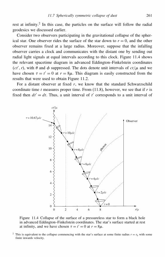
11.7 Spherically symmetric collapse of dust 261
rest at infinity.2 In this case, the particles on the surface will follow the radialgeodesics we discussed earlier.
Consider two observers participating in the gravitational collapse of the spher-ical star. One observer rides the surface of the star down to r = 0, and the otherobserver remains fixed at a large radius. Moreover, suppose that the infallingobserver carries a clock and communicates with the distant one by sending outradial light signals at equal intervals according to this clock. Figure 11.4 showsthe relevant spacetime diagram in advanced Eddington–Finkelstein coordinatesct′ r, with and suppressed. The dots denote unit intervals of ct/ and wehave chosen = t′ = 0 at r = 8. This diagram is easily constructed from theresults that were used to obtain Figure 11.2.
For a distant observer at fixed r, we know that the standard Schwarzschildcoordinate time t measures proper time. From (11.8), however, we see that if r isfixed then dt′ = dt. Thus, a unit interval of t′ corresponds to a unit interval of
r/µ
ct'/µ
2
4
6
8
14
10
12
2 4 6 80
0
τ = 10.67µ /c
τ = 8µ /c
τ = 6µ /c
τ = 4µ /c
τ = 2µ /c
τ = 0
phot
on
Observer
τ = 10µ /c
Figure 11.4 Collapse of the surface of a pressureless star to form a black holein advanced Eddington–Finkelstein coordinates. The star’s surface started at restat infinity, and we have chosen = t′ = 0 at r = 8.
2 This is equivalent to the collapse commencing with the star’s surface at some finite radius r = r0 with somefinite inwards velocity.
262 Schwarzschild black holes
proper time for a distant fixed observer. From the diagram, we see that the lightpulses are not received at equal intervals of t′. Rather, the proper time intervalmeasured by the distant observer between each pulse steadily increases. Indeed,the last light pulse to reach this observer is the one emitted just before the surfaceof the star crosses r = 2. The worldine of this photon is simply the vertical liner = 2, and so this pulse would only ‘reach’ the distant observer at t=. Pulsesemitted after the surface of the star has crossed the event horizon do not progressto larger r but instead progress to smaller r and end up at the singularity at r = 0.
Thus, the distant observer never sees the star’s surface cross the radius r = 2.Furthermore, the pulses emitted at equal intervals by the falling observer’s clockarrive at the distant observer at increasingly longer intervals. Correspondingly, thephotons received by the distant observer are increasingly redshifted, the redshifttending to infinity as the star’s surface approaches r = 2. Both these effectsmean that the distant observer sees the luminosity of the star fall to zero. Tosummarise, the distant observer sees the collapse slow down and the star’s stateapproach that of a quasi-equilibrium object with radius r = 2, which eventuallybecomes totally dark. Thus, the distant observer sees the formation of a black hole.
Let us quantify further what the observer sees as the star collapses to forma black hole. Since we are interested in measurements made by a distantfixed observer, we may use either advanced Eddington–Finkelstein coordinatest′ r or traditional Scharwzschild coordinates t r , as both correspondto physical quantities at large r. We shall use the latter simply because wehave already obtained the equations for a massive radially infalling particle inSchwarzschild coordinates. Suppose that a particle on the surface of the star emitsa radially outgoing pulse of light at coordinates tE rE, which is received by thedistant fixed observer at tR rR. Since the photon follows a radially outgoingnull geodesic, we can write
ctE− rE−2 ln
∣∣∣∣ rE2 −1
∣∣∣∣= ctR− rR−2 ln
∣∣∣∣ rR2 −1
∣∣∣∣ (11.12)
The radial coordinate ‘seen’ by the distant observer at time tR is the functionrEtR obtained by solving (11.12). Using the fact that the coordinates tE and rE ofthe freely falling emitter are related by (11.4), we find that, if r is very close to 2,
rEtR≈ 2+a exp(−ctR4
) (11.13)
where a is an unimportant constant depending on and rR. The importantconsequence of this result is that the radius r = 2 is approached exponentially,as seen by the distant observer, with a characteristic time 4/c. Since
c= GM
c3= 5×10⁻⁶
(M
M
)seconds
11.7 Spherically symmetric collapse of dust 263
the time scale for stellar-size objects is very small by the usual astrophysicalstandards. Thus for any collapse even approximately like the free-fall collapsedescribed here, the approach to a black hole is extremely rapid.
Let us work out the redshift seen by the distant observer as a function of time t.The ratio of the frequencies of a photon at emission and reception is
RE= u
RpR
uEpE
(11.14)
where uE and uR are the 4-velocities of the emitter and receiver respectively andp is the photon 4-momentum. The 4-velocity of our emitter riding on the star’ssurface is [
uE
]= 1−2/r−1−2c2/r1/200whereas the 4-velocity of the stationary observer at infinity is[
uR
]= 1000
Hence (11.14) reduces to
RE= p0R
u0Ep0E+u1Ep1E=[u0E+
p1E
p0Eu1E
]−1
where we have used that fact that the Schwarzschild metric is stationary and sop0 is conserved along the photon geodesic. Moreover, since p is null we requiregpp = 0, which in our case reduces to
1c2
(1− 2
r
)−1p0
2−(1− 2
r
)p1
2 = 0
So, for a radially outgoing photon, p1 =−1−2/r−1p0/c and we find that
RE=(1− 2
r
)[1+
(2r
)1/2]−1
= 1−(2r
)1/2
(11.15)
As r→ 2 we see that R→ 0, so the redshift is infinite. By Taylor-expanding(11.15) about r = 2, we find that for r close to 2 we can write
RE≈ r−2
4
however, near the event horizon the time of reception is given by (11.13). Hence
RE∼ exp
(− ct
4
)
264 Schwarzschild black holes
so that the redshift goes exponentially to infinity with a characteristic time 4/c.The computation of the luminosity is more complicated since it involves non-radialphoton geodesics also. Nevertheless, using the above analysis we see that the timeintervals between successive photons will also decrease as ∼ exp −ct/4 andso we expect the luminosity to decay exponentially as ∼ exp −ct/2.
11.8 Tidal forces near a black hole
As discussed in Section 7.14, in Newtonian gravity a distribution of non-interacting particles freely falling towards the Earth will be elongated in thedirection of motion and compressed in the transverse directions, as a result ofgravitational tidal forces. The same effect occurs in a body falling towards aspherical object in general relativity, but if the object is a black hole then theeffect becomes infinite at r = 0.
We may calculate the tidal forces in the Schwarzschild geometry, working intraditional Schwarzschild coordinates t r . At any particular point in space,the tidal forces have the same form for any (close) pair of particles that are infree fall. Thus, it is easiest to calculate the tidal forces at some coordinate radiusr for the case in which the two particles are released from rest at r. In this case, aframe of orthonormal basis vectors defining the inertial instantaneous rest frameof one of the particles may be taken as
e0 = 1
cu = 1
c
(1− 2
r
)−1/20 e1
=(1− 2
r
)1/2
1
e2 = 1
r2 e3
= 1r sin
3
Substituting these expressions into (7.28), together with the appropriate expres-sions for the components of the Riemann tensor in Schwarzschild coordinates,from (7.27) we obtain (after some algebra) that the spatial components of theorthogonal connecting vector between the two particles satisfy
d2r
d2=+2c2
r3r
d2
d2=−c2
r3
d2
d2=−c2
r3
The positive sign in the r -equation indicates a tension or stretching in the radialdirection and the negative signs in the - and - equations indicate a pressure orcompression in the transverse directions. Note the 1/r3 radial dependence in eachcase, which is characteristic of tidal gravitational forces. Moreover, the equationsreveal that the tidal forces do not undergo any ‘transition’ at r = 2 but becomeinfinite at r = 0.
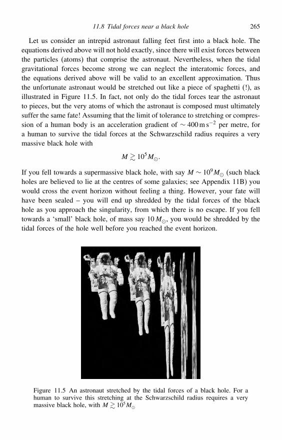
11.8 Tidal forces near a black hole 265
Let us consider an intrepid astronaut falling feet first into a black hole. Theequations derived above will not hold exactly, since there will exist forces betweenthe particles (atoms) that comprise the astronaut. Nevertheless, when the tidalgravitational forces become strong we can neglect the interatomic forces, andthe equations derived above will be valid to an excellent approximation. Thusthe unfortunate astronaut would be stretched out like a piece of spaghetti (!), asillustrated in Figure 11.5. In fact, not only do the tidal forces tear the astronautto pieces, but the very atoms of which the astronaut is composed must ultimatelysuffer the same fate! Assuming that the limit of tolerance to stretching or compres-sion of a human body is an acceleration gradient of ∼ 400m s−2 per metre, fora human to survive the tidal forces at the Schwarzschild radius requires a verymassive black hole with
M 105M
If you fell towards a supermassive black hole, with say M ∼ 109M (such blackholes are believed to lie at the centres of some galaxies; see Appendix 11B) youwould cross the event horizon without feeling a thing. However, your fate willhave been sealed – you will end up shredded by the tidal forces of the blackhole as you approach the singularity, from which there is no escape. If you felltowards a ‘small’ black hole, of mass say 10M, you would be shredded by thetidal forces of the hole well before you reached the event horizon.
Figure 11.5 An astronaut stretched by the tidal forces of a black hole. For ahuman to survive this stretching at the Schwarzschild radius requires a verymassive black hole, with M 105M
266 Schwarzschild black holes
11.9 Kruskal coordinates
In our discussion of advanced and retarded Eddington–Finkelstein coordinates, wefound that neither coordinate system was completely satisfactory. In the advancedcoordinates the outgoing null rays are discontinuous, and in the retarded coor-dinates the ingoing null rays are discontinuous. It is natural to ask whether it ispossible to find a system of coordinates in which both the incoming and outgoingradial photon geodesics are continuous straight lines. Such a coordinate systemwas indeed discovered in 1961 by Martin Kruskal, and it serves also to clarifythe structure of the complete Schwarzschild geometry.
An obvious way to begin is to introduce both the advanced null coordinate p
and the retarded null coordinate q that we met during our discussion of Eddington–Finkelstein coordinates. In the coordinates p q the Schwarzschild metricbecomes
ds2 =(1− 2
r
)dpdq− r2d2+ sin2 d2 (11.16)
where r is considered as a function of p and q, defined implicitly by
12p−q= r+2 ln
∣∣∣∣ r2 −1
∣∣∣∣ Our new system of coordinates has some appealing properties. Most impor-
tantly, the 2-space defined by = constant, = constant has the simple metric
ds2 =(1− 2
r
)dpdq (11.17)
Transforming from the null coordinates p and q to the new coordinates
ct = 12p+q (11.18)
r = 12p−q= r+2 ln
∣∣∣∣ r2 −1
∣∣∣∣ (11.19)
where t is the standard Schwarzschild timelike coordinate and r is a radial space-like coordinate (sometimes called the tortoise coordinate!), the 2-space metricthen becomes
ds2 =(1− 2
r
)(c2 dt2−dr2
)(11.20)
= 2x dx dx (11.21)
where x0 = ct and x1 = r. This line element has the same form as that of aMinkowski 2-space (which is spatially flat) but it is multiplied by what mathemati-cians call a conformal scaling factor, 2x, which is a function of position. The
11.9 Kruskal coordinates 267
2-space itself is curved, because the derivatives of the functionx enter into thecomponents of the curvature tensor, but the line element (11.21) of the 2-spaceis manifestly conformally flat. In fact, any two-dimensional (pseudo-)Riemannianmanifold is conformally flat (see Appendix 11C), in that a coordinate systemalways exists in which the line element takes the form (11.21). We have thussucceeded in finding such a coordinate system for the 2-space (11.17).
The form of the line element (11.21) has an important consequence for studyingthe paths of radially moving photons (for which d=d= 0). Since the conformalfactor 2x is just a scaling, it does not change the lightcone structure and sothe latter should just look like that in Minkowski space. Thus, in a spacetimediagram in ct r coordinates, both ingoing and outgoing radial null geodesicsare straight lines with slope ±1, as is easily seen by setting ds2 = 0 in (11.20).Unfortunately, however, the coordinates ct r are pathological when r = 2,
as is easily seen from (11.19). This suggests that, instead of using the parametersp and q directly, we should look for a coordinate transformation that preservesthe manifest conformal nature of the 2-space defined by (11.17) but removes theoffending factor 1− 2/r, which is the cause of the pathological behaviour. Itis straightforward to see that a transformation of the form pp and qq willachieve this goal, since, in this case, the metric becomes
ds2 =(1− 2
r
)dp
dp
dq
dqdpdq
which has the same general form as (11.17). An appropriate choice of the functionspp and qq that removes the factor 1− 2/r in the line element is (assuggested by Kruskal)
p= exp(
p
4
) q =− exp
(− q
4
)
for which we find that
ds2 = 323
rexp
(− r
2
)dpdq
The usual form of the metric is then obtained by defining a timelike variable v
and a spacelike variable u by
v= 12 p+ q u= 1
2 p− q
Thus, the full line element for the Schwarzschild geometry in Kruskal coordinatesvu is given by
ds2 = 323
rexp
(− r
2
)(dv2−du2
)− r2d2+ sin2 d2 (11.22)
268 Schwarzschild black holes
where r is considered as a function of v and u that is defined implicitly by
u2−v2 =(
r
2−1
)exp
(r
2
) (11.23)
It is straightforward to show that the coordinates v and u are related to theoriginal Schwarzschild coordinates t and r by the following transformations. Forr > 2 we have
v =(
r
2−1
)1/2
exp(
r
4
)sinh
(ct
4
)
u =(
r
2−1
)1/2
exp(
r
4
)cosh
(ct
4
)
whereas, for r < 2,
v =(1− r
2
)1/2
exp(
r
4
)cosh
(ct
4
)
u =(1− r
2
)1/2
exp(
r
4
)sinh
(ct
4
)
Considerable insight into the nature of the Schwarzschild geometry can beobtained by plotting its spacetime diagram in Kruskal coordinates. The causalstructure defined by radial light rays is (by construction) particularly easy toanalyse in Kruskal coordinates. From the metric (11.22), we see that for ds =d = d= 0 we have
v=±u+ constant
which represents straight lines at ±45 to the axes. This is a direct consequence ofthe fact that the 2-space with d= d= 0 is manifestly conformally flat in vucoordinates. Thus, the lightcone structure should look like that in Minkowskispace. Also, we note that a massive particle worldline must always lie within thefuture light-cone at each point.
It is also instructive to plot lines of constant t and r. From (11.23) we see thatlines of constant r are curves of constant u2− v2 and are hence hyperbolae. Inparticular, the value r = 2 correpsonds to either of the straight lines u = ±v,which are the asymptotes to the set of constant-r hyperbolae, and the value r = 0corresponds to the hyperbolae v = ±√u2+1. Thus the ‘point’ in space r = 0is mapped into two lines. However, not too much can be made of this since itis a singularity of the geometry. We should not glibly speak of it as a part of
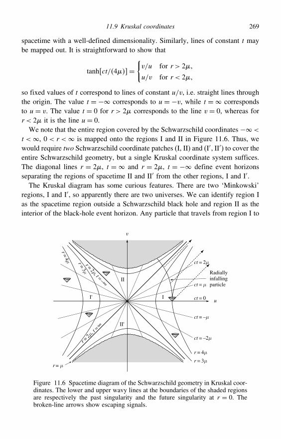
11.9 Kruskal coordinates 269
spacetime with a well-defined dimensionality. Similarly, lines of constant t maybe mapped out. It is straightforward to show that
tanh ct/4=v/u for r > 2
u/v for r < 2
so fixed values of t correspond to lines of constant u/v, i.e. straight lines throughthe origin. The value t = − corresponds to u = −v, while t = correspondsto u = v. The value t = 0 for r > 2 corresponds to the line v = 0, whereas forr < 2 it is the line u= 0.
We note that the entire region covered by the Schwarzschild coordinates −<
t <, 0 < r < is mapped onto the regions I and II in Figure 11.6. Thus, wewould require two Schwarzschild coordinate patches (I, II) and (I′ II′) to cover theentire Schwarzschild geometry, but a single Kruskal coordinate system suffices.The diagonal lines r = 2, t = and r = 2, t = − define event horizonsseparating the regions of spacetime II and II′ from the other regions, I and I′.The Kruskal diagram has some curious features. There are two ‘Minkowski’
regions, I and I′, so apparently there are two universes. We can identify region Ias the spacetime region outside a Schwarzschild black hole and region II as theinterior of the black-hole event horizon. Any particle that travels from region I to
r = µ
I
IIRadiallyinfallingparticle
I'
II'
ct = 2µ
ct = µ
ct = –2µ
ct = –µ
r = 4µr = 3µ
r=4µ r=
3µr=
2µ, t = –∞
ct = 0
v
u
r=2µ , t
= ∞
Figure 11.6 Spacetime diagram of the Schwarzschild geometry in Kruskal coor-dinates. The lower and upper wavy lines at the boundaries of the shaded regionsare respectively the past singularity and the future singularity at r = 0. Thebroken-line arrows show escaping signals.
270 Schwarzschild black holes
region II can never return and, moreover, must eventually reach the singularityr = 0. Regions I′ and II′ are completely inaccessible from regions I or II. RegionII′ is similar to region II but in reverse: it is a part of spacetime from whicha particle can escape (into regions I and I′) but not enter. Moreover, there isa singularity in the past – a white hole – from which particles can emanate.Indeed, we may now understand more clearly our discussion of the advancedand retarded Eddington–Finkelstein coordinates in Section 11.5: the advancedcoordinates describe the Schwarzschild geometry in regions I and II, whereas theretarded coordinates cover the regions I′ and II′. The two universes I and I′ areactually connected by a wormhole at the origin, which we discuss in more detailin the next section, but, as we will show, no particle can travel between regionsI and I′.
It is worth asking what has happened here. How can a few simple coordinatetransformations lead to what is apparently new physics? What we have doneamounts to mathematically extending the Schwarzschild solution. Mathematicianswould call this a maximal extension of the Schwarzschild solution because allgeodesics either extend to infinite values of their affine parameter or end at apast or future singularity. Thus Kruskal coordinates probe all the Schwarzschildgeometry. Hence, we find that the complete Schwarzschild geometry consists ofa black hole and white hole and two universes connected at their horizons by awormhole.
The extended Schwarzschild metric is a solution of Einstein’s theory and henceis allowed by classical general relativity. Thus, for example, classical generalrelativity allows the existence of white holes. Photons or particles could, inprinciple, emanate from a past singularity. But, as you can see from the Kruskalspacetime diagram, you cannot ‘fall into’ a white hole since it can only exist inyour past. Can a white hole really exist? The answer is that we don’t know forsure. Classical GR must break down at singularities. We would expect quantumeffects to become important at ultra-short distances and ultra-high energies. Infact, from the three fundamental constants G, and c we can form the followingenergy, mass, time, length and density scales:
Planck energy EP =(c5/G
)1/2 = 122×1019 GeV
Planck mass mP = c/G1/2 = 218×10−5 g
Planck time tP =(G/c5
)1/2 = 539×10−44 s
Plancklength lP =(G/c3
)1/2 = 162×10−33 cm
Planck density P =(c5/G2
)= 516×1093 g cm−3
11.10 Wormholes and the Einstein–Rosen bridge 271
These Planck scales define the characteristic energies, lengths, times, etc. at whichwe expect quantum gravitational effects to become important. To put it into somekind of perspective, an elementary particle with the Planck mass would weighabout the same as a small bacterium.
Nobody really expects the centres of black holes to harbour true singularities.Instead, it is expected that, close to the classical singularity, quantum gravitationaleffects will occur that will prevent the divergences of classical general relativity.We do not yet have a complete theory of quantum gravity, though many peoplehope that M-theory (formerly known as superstring theory) might one day providesuch a theory. Theorists have developed semi-classical theories, however, whichmight (or might not) contain some of the features of a complete theory of quantumgravity. Such calculations suggest that white holes would be unstable and couldnot exist for more than about a Planck time. It is interesting that within a fewpages we have pushed Einstein’s theory of gravity to the edge of known physics.
11.10 Wormholes and the Einstein–Rosen bridge
Although it is not obvious from Figure 11.6, the two universes I and I′ are actuallyconnected by a wormhole at the origin. To understand the structure at the origin,you must realize that the coordinates and have been suppressed in this figure;each point in Figure 11.6 actually represents a 2-sphere.
We can gain some intuitive insight into wormholes by considering the geometryof the spacelike hypersurface v = 0, which extends from u = + to u = −.The line element for this hypersurface is
ds2 =−323
rexp
(− r
2
)du2− r2d2+ sin2 d2
We can draw a cross-section of this hypersurface corresponding to the equatorialplane = /2, in which the line element reduces further to
ds2 =−323
rexp
(− r
2
)du2− r2 d2 (11.24)
To interpret this, we may consider a two-dimensional surface possessing aline element d#2 given by minus (11.24) and embed it in a three-dimensionalEuclidean space.
This embedding is most easily performed by re-expressing d#2 in terms of thecoordinates r and , which is easily shown to yield the familiar form
d#2 =(1− 2
r
)−1dr2+ r2 d2 (11.25)
272 Schwarzschild black holes
However, we must remember that, in the spacelike hypersurface v = 0, as wemove along the u-axis from + to − the value of r decreases to a minimumvalue r = 2 (at u= 0) and then increases again. In general, in Euclidean space, a2-surface parameterised by arbitrary coordinates can be specified by givingthree functions xaa= 123, where the xa define some coordinate systemin the three-dimensional Euclidean space. In our particular case, it will be usefulto use cylindrical polar coordinates z, in which case the line element ofthe three-dimensional space is
d#2 = d2+2 d2+dz2 (11.26)
Moreover, since the 2-surface we wish to embed (which is parameterised by thecoordinates r and ) is clearly axisymmetric, we may take the three functionsspecifying this surface to have the form
= r = z= zr
Substituting these forms into (11.26), we may thus write the line element on theembedded 2-surface as
d#2 =[(
d
dr
)2
+(dz
dr
)2]dr2+2 d2 (11.27)
For the geometry of the embedded 2-surface to be identical to the geometry ofthe 2-space of interest, we require the line elements (11.25) and (11.27) to beidentical, and so we require r= r and thus
1+(dz
dr
)2
=(1− 2
r
)−1
The solution to this differential equation is easily found to be
zr=√8r−2+ constant
and substituting r = gives us the equation of the cross-section of the embedded2-surface in the z-plane of the Euclidean 3-space. Taking the constant ofintegration to be zero, and remembering that r (and hence ) is never less than2, we find that the surface has the form shown in Figure 11.7. Thus, thegeometry of the spacelike hypersurface at v= 0 can be thought of as two distinct,but identical, asymptotically flat Schwarzschild manifolds joined at the ‘throat’r = 2 by an Einstein–Rosen bridge. If one so wishes, one can also connect thetwo asymptotically flat regions together in a region distant from the throat. In thiscase, the wormhole connects two distant regions of a single universe.
In either case, the structure of the wormhole is dynamic. One is used to thinkingof the Schwarzschild geometry as ‘static’. However, working for the moment in
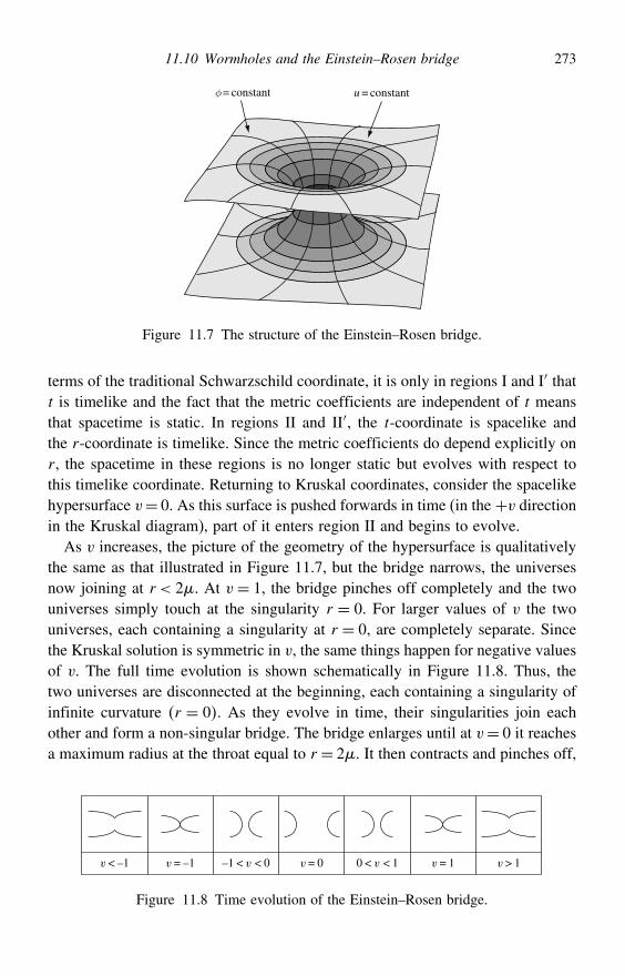
11.10 Wormholes and the Einstein–Rosen bridge 273
φ = constant u = constant
Figure 11.7 The structure of the Einstein–Rosen bridge.
terms of the traditional Schwarzschild coordinate, it is only in regions I and I′ thatt is timelike and the fact that the metric coefficients are independent of t meansthat spacetime is static. In regions II and II′, the t-coordinate is spacelike andthe r-coordinate is timelike. Since the metric coefficients do depend explicitly onr, the spacetime in these regions is no longer static but evolves with respect tothis timelike coordinate. Returning to Kruskal coordinates, consider the spacelikehypersurface v= 0. As this surface is pushed forwards in time (in the +v directionin the Kruskal diagram), part of it enters region II and begins to evolve.
As v increases, the picture of the geometry of the hypersurface is qualitativelythe same as that illustrated in Figure 11.7, but the bridge narrows, the universesnow joining at r < 2. At v = 1, the bridge pinches off completely and the twouniverses simply touch at the singularity r = 0. For larger values of v the twouniverses, each containing a singularity at r = 0, are completely separate. Sincethe Kruskal solution is symmetric in v, the same things happen for negative valuesof v. The full time evolution is shown schematically in Figure 11.8. Thus, thetwo universes are disconnected at the beginning, each containing a singularity ofinfinite curvature r = 0. As they evolve in time, their singularities join eachother and form a non-singular bridge. The bridge enlarges until at v= 0 it reachesa maximum radius at the throat equal to r = 2. It then contracts and pinches off,
v< –1 v= –1 –1 < v < 0 0 < v < 1 v> 1v= 0 v= 1
Figure 11.8 Time evolution of the Einstein–Rosen bridge.
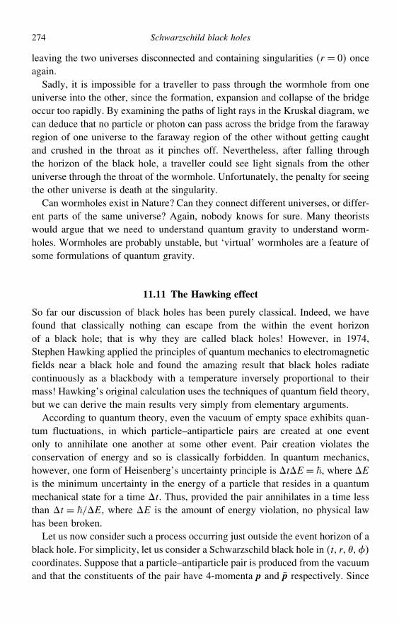
274 Schwarzschild black holes
leaving the two universes disconnected and containing singularities r = 0 onceagain.
Sadly, it is impossible for a traveller to pass through the wormhole from oneuniverse into the other, since the formation, expansion and collapse of the bridgeoccur too rapidly. By examining the paths of light rays in the Kruskal diagram, wecan deduce that no particle or photon can pass across the bridge from the farawayregion of one universe to the faraway region of the other without getting caughtand crushed in the throat as it pinches off. Nevertheless, after falling throughthe horizon of the black hole, a traveller could see light signals from the otheruniverse through the throat of the wormhole. Unfortunately, the penalty for seeingthe other universe is death at the singularity.
Can wormholes exist in Nature? Can they connect different universes, or differ-ent parts of the same universe? Again, nobody knows for sure. Many theoristswould argue that we need to understand quantum gravity to understand worm-holes. Wormholes are probably unstable, but ‘virtual’ wormholes are a feature ofsome formulations of quantum gravity.
11.11 The Hawking effect
So far our discussion of black holes has been purely classical. Indeed, we havefound that classically nothing can escape from the within the event horizonof a black hole; that is why they are called black holes! However, in 1974,Stephen Hawking applied the principles of quantum mechanics to electromagneticfields near a black hole and found the amazing result that black holes radiatecontinuously as a blackbody with a temperature inversely proportional to theirmass! Hawking’s original calculation uses the techniques of quantum field theory,but we can derive the main results very simply from elementary arguments.
According to quantum theory, even the vacuum of empty space exhibits quan-tum fluctuations, in which particle–antiparticle pairs are created at one eventonly to annihilate one another at some other event. Pair creation violates theconservation of energy and so is classically forbidden. In quantum mechanics,however, one form of Heisenberg’s uncertainty principle is tE = , where Eis the minimum uncertainty in the energy of a particle that resides in a quantummechanical state for a time t. Thus, provided the pair annihilates in a time lessthan t = /E, where E is the amount of energy violation, no physical lawhas been broken.
Let us now consider such a process occurring just outside the event horizon of ablack hole. For simplicity, let us consider a Schwarzschild black hole in t r coordinates. Suppose that a particle–antiparticle pair is produced from the vacuumand that the constituents of the pair have 4-momenta p and p respectively. Since
11.11 The Hawking effect 275
the spacetime is stationary 0g = 0, the quantities p0 = e0 ·p and p0 = e0 · p areconserved along the particle worldlines; here e0 is the t-coordinate basis vector.Thus, for a fluctuation from the vacuum, classical conservation requires
e0 ·p+ e0 · p= 0 (11.28)
The squared ‘length’ of the coordinate basis vector e0 is given by
e0 · e0 = g00 = c21−2/r (11.29)
Thus, outside the horizon r > 2, e0 is timelike. The components e0 ·p and e0 · pare therefore proportional to the particle energies as measured by an observerwhose 4-velocity is along the e0-direction. Hence both must be positive, so theconservation condition (11.28) cannot be satisfied.
However, if the fluctuation occurs near the event horizon then the inward-moving particle may travel to the region r < 2. Inside the event horizon e0is spacelike, as shown by (11.29). Thus e0 · p is a component of the spatialmomentum for some observer and so may be negative. Hence the conservationcondition (11.28) can be satisfied if the antiparticle (say) crosses the horizon withnegative e0 · p and the particle escapes to infinity with positive e0 ·p. As seen byan observer at infinity, the black hole has emitted a particle of energy e0 ·p andthe black hole’s mass has decreased by e0 · pc2 as a consequence of the particlefalling into it. This is the Hawking effect. Of course, the argument is equally validif it is the particle that falls into the black hole and the antiparticle that escapesto infinity. The black hole emits particles and antiparticles in equal numbers.
For a fluctuation near the horizon, the inward-travelling particle needs to endurein a prohibited negative e0 ·p condition only for a short proper time, as measured bysome locally free-falling observer, before reaching the inside of the horizon wherenegative e0 ·p is allowed. The particle has, in fact, tunnelled quantum mechanicallythrough a region outside the horizon, where negative e0 ·p is classically forbidden,to a region inside the event horizon where it is classically allowed. The processworks best where the proper time in the forbidden region is smallest, i.e. close tothe horizon.
The distant observer sees a steady flux of particles and antiparticles. The fluxmust be steady, since the geometry is independent of t and so the rate of particleemission must also be independent of t. Let us calculate the typical energy ofsuch a particle as measured by the distant observer. Suppose that the particle–antiparticle pair is created at some event P with coordinate radius R= 2+. Letus consider this event as viewed by a freely falling observer, starting from rest atthis point. Since the observer is in free fall, the rules of special relativity apply inhis frame. A typical measure of the proper time elapsed before the observer
276 Schwarzschild black holes
reaches the horizon may be obtained by considering a radially free-falling particlethat starts from rest at r = R. In this case,
t = 1−2/R1/2
1−2/r
r = −[2c2
(1r− 1R
)]1/2
Thus the required proper time interval is
=−∫ 2
2+
(2c2
r− 2c2
2+
)−1/2dr ≈ 221/2
c
where the final result is quoted to first order in . From the uncertainty principle,the typical energy of the particle, as measured by a freely falling observer, isgiven by
=
= c
22−1/2
However, this can also be written as
= p ·u≈ p0u0
where u is the observer’s 4-velocity and the approximation holds since u1 u0.Now, u0 = t ≈ 2/1/2 to first order in . Moreover, p0 is conserved alongthe particle’s worldline and is equal to the energy E of the particle as measuredby the distant observer, whose 4-velocity is simply u= 1000. Thus, wefinally obtain
E =
(
2
)1/2
= c3
4GM (11.30)
Remarkably, this result does not depend on ; the particle always emerges withthis characteristic energy.
The full quantum field theory calculation shows that the particles are infact received with a blackbody energy spectrum characterised by the Hawkingtemperature
T = c3
8kBGM
The typical particle energy is thus E = kBT = c3/8GM, which is only afactor 2 smaller than our crude estimate (11.30). Putting in numbers, we find that
T = 6×10⁻⁸(
M
M
)−1K
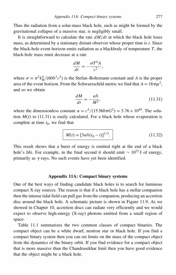
Appendix 11A: Compact binary systems 277
Thus the radiation from a solar-mass black hole, such as might be formed by thegravitational collapse of a massive star, is negligibly small.
It is straightforward to calculate the rate dM/dt at which the black hole losesmass, as determined by a stationary distant observer whose proper time is t. Sincethe black-hole event horizon emits radiation as a blackbody of temperature T , theblack-hole mass must decrease at a rate
dM
dt=−#T 4A
c2
where # = 2k4B/603c2 is the Stefan–Boltzmann constant and A is the proper
area of the event horizon. From the Schwarzschild metric we find that A= 162,and so we obtain
dM
dt=−
M2 (11.31)
where the dimensionless constant = c4/15360G2= 376×1049. The solu-tion Mt to (11.31) is easily calculated. For a black hole whose evaporation iscomplete at time t0, we find that
Mt= 3t0− t1/3 (11.32)
This result shows that a burst of energy is emitted right at the end of a blackhole’s life. For example, in the final second it should emit ∼ 1022 J of energy,primarily as -rays. No such events have yet been identified.
Appendix 11A: Compact binary systems
One of the best ways of finding candidate black holes is to search for luminouscompact X-ray sources. The reason is that if a black hole has a stellar companionthen the intense tidal field can pull gas from the companion, producing an accretiondisc around the black hole. A schematic picture is shown in Figure 11.9. As weshowed in Chapter 10, accretion discs can radiate very efficiently and we wouldexpect to observe high-energy (X-ray) photons emitted from a small region ofspace.
Table 11.1 summarizes the two common classes of compact binaries. Thecompact object can be a white dwarf, neutron star or black hole. If you find acompact binary system then you can set limits on the mass of the compact objectfrom the dynamics of the binary orbit. If you find evidence for a compact objectthat is more massive than the Chandrasekhar limit then you have good evidencethat the object might be a black hole.
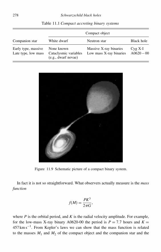
278 Schwarzschild black holes
Table 11.1 Compact accreting binary systems
Compact object
Companion star White dwarf Neutron star Black hole
Early type, massive None known Massive X-ray binaries Cyg X-ILate type, low mass Cataclysmic variables
(e.g., dwarf novae)Low mass X-ray binaries A0620−00
Figure 11.9 Schematic picture of a compact binary system.
In fact it is not so straightforward. What observers actually measure is the massfunction
fM= PK3
2G
where P is the orbital period, and K is the radial velocity amplitude. For example,for the low-mass X-ray binary A0620-00 the period is P = 77 hours and K =457km s−1. From Kepler’s laws we can show that the mass function is relatedto the masses M1 and M2 of the compact object and the companion star and the
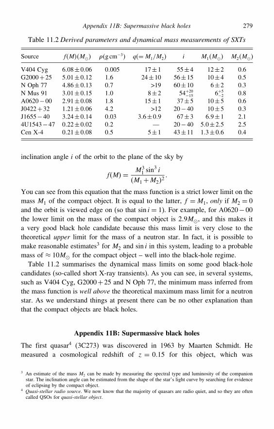
Appendix 11B: Supermassive black holes 279
Table 11.2 Derived parameters and dynamical mass measurements of SXTs
Source fMM gcm−3 q=M1/M2 i M1M M2M
V404 Cyg 608±006 0005 17±1 55±4 12±2 0.6G2000+25 501±012 16 24±10 56±15 10±4 0.5N Oph 77 486±013 07 >19 60±10 6±2 0.3N Mus 91 301±015 10 8±2 54+20−15 6+5−2 0.8A0620−00 291±008 18 15±1 37±5 10±5 0.6J0422+32 121±006 42 >12 20−40 10±5 0.3J1655−40 324±014 003 36±09 67±3 69±1 2.14U1543−47 022±002 02 — 20−40 50±25 2.5Cen X-4 021±008 05 5±1 43±11 13±06 0.4
inclination angle i of the orbit to the plane of the sky by
fM= M31 sin
3 i
M1+M22
You can see from this equation that the mass function is a strict lower limit on themass M1 of the compact object. It is equal to the latter, f =M1, only if M2 = 0and the orbit is viewed edge on (so that sin i= 1). For example, for A0620−00the lower limit on the mass of the compact object is 29M, and this makes ita very good black hole candidate because this mass limit is very close to thetheoretical upper limit for the mass of a neutron star. In fact, it is possible tomake reasonable estimates3 for M2 and sin i in this system, leading to a probablemass of ≈ 10M for the compact object – well into the black-hole regime.
Table 11.2 summarises the dynamical mass limits on some good black-holecandidates (so-called short X-ray transients). As you can see, in several systems,such as V404 Cyg, G2000+25 and N Oph 77, the minimum mass inferred fromthe mass function is well above the theoretical maximum mass limit for a neutronstar. As we understand things at present there can be no other explanation thanthat the compact objects are black holes.
Appendix 11B: Supermassive black holes
The first quasar4 (3C273) was discovered in 1963 by Maarten Schmidt. Hemeasured a cosmological redshift of z = 015 for this object, which was
3 An estimate of the mass M2 can be made by measuring the spectral type and luminosity of the companionstar. The inclination angle can be estimated from the shape of the star’s light curve by searching for evidenceof eclipsing by the compact object.
4 Quasi-stellar radio source. We now know that the majority of quasars are radio quiet, and so they are oftencalled QSOs for quasi-stellar object.
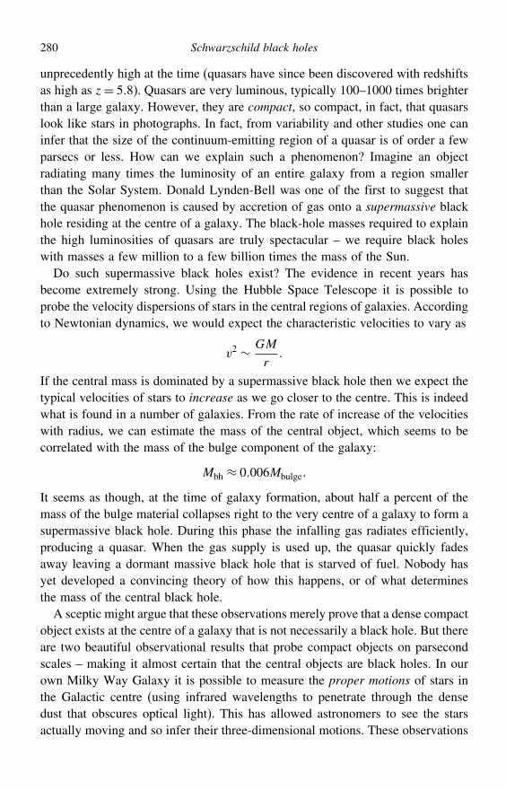
280 Schwarzschild black holes
unprecedently high at the time (quasars have since been discovered with redshiftsas high as z= 58). Quasars are very luminous, typically 100–1000 times brighterthan a large galaxy. However, they are compact, so compact, in fact, that quasarslook like stars in photographs. In fact, from variability and other studies one caninfer that the size of the continuum-emitting region of a quasar is of order a fewparsecs or less. How can we explain such a phenomenon? Imagine an objectradiating many times the luminosity of an entire galaxy from a region smallerthan the Solar System. Donald Lynden-Bell was one of the first to suggest thatthe quasar phenomenon is caused by accretion of gas onto a supermassive blackhole residing at the centre of a galaxy. The black-hole masses required to explainthe high luminosities of quasars are truly spectacular – we require black holeswith masses a few million to a few billion times the mass of the Sun.
Do such supermassive black holes exist? The evidence in recent years hasbecome extremely strong. Using the Hubble Space Telescope it is possible toprobe the velocity dispersions of stars in the central regions of galaxies. Accordingto Newtonian dynamics, we would expect the characteristic velocities to vary as
v2 ∼ GM
r
If the central mass is dominated by a supermassive black hole then we expect thetypical velocities of stars to increase as we go closer to the centre. This is indeedwhat is found in a number of galaxies. From the rate of increase of the velocitieswith radius, we can estimate the mass of the central object, which seems to becorrelated with the mass of the bulge component of the galaxy:
Mbh ≈ 0006Mbulge
It seems as though, at the time of galaxy formation, about half a percent of themass of the bulge material collapses right to the very centre of a galaxy to form asupermassive black hole. During this phase the infalling gas radiates efficiently,producing a quasar. When the gas supply is used up, the quasar quickly fadesaway leaving a dormant massive black hole that is starved of fuel. Nobody hasyet developed a convincing theory of how this happens, or of what determinesthe mass of the central black hole.
A sceptic might argue that these observations merely prove that a dense compactobject exists at the centre of a galaxy that is not necessarily a black hole. But thereare two beautiful observational results that probe compact objects on parsecondscales – making it almost certain that the central objects are black holes. In ourown Milky Way Galaxy it is possible to measure the proper motions of stars inthe Galactic centre (using infrared wavelengths to penetrate through the densedust that obscures optical light). This has allowed astronomers to see the starsactually moving and so infer their three-dimensional motions. These observations
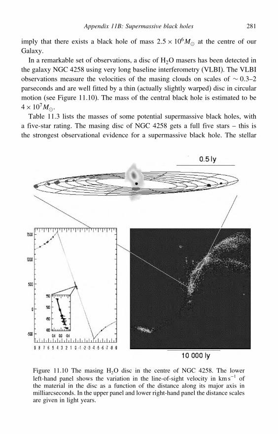
Appendix 11B: Supermassive black holes 281
imply that there exists a black hole of mass 25× 106M at the centre of ourGalaxy.
In a remarkable set of observations, a disc of H2O masers has been detected inthe galaxy NGC 4258 using very long baseline interferometry (VLBI). The VLBIobservations measure the velocities of the masing clouds on scales of ∼ 03–2parseconds and are well fitted by a thin (actually slightly warped) disc in circularmotion (see Figure 11.10). The mass of the central black hole is estimated to be4×107M.
Table 11.3 lists the masses of some potential supermassive black holes, witha five-star rating. The masing disc of NGC 4258 gets a full five stars – this isthe strongest observational evidence for a supermassive black hole. The stellar
Figure 11.10 The masing H2O disc in the centre of NGC 4258. The lowerleft-hand panel shows the variation in the line-of-sight velocity in km s−1 ofthe material in the disc as a function of the distance along its major axis inmilliarcseconds. In the upper panel and lower right-hand panel the distance scalesare given in light years.
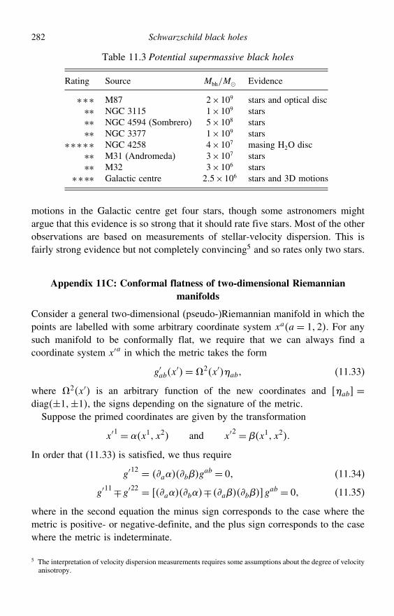
282 Schwarzschild black holes
Table 11.3 Potential supermassive black holes
Rating Source Mbh/M Evidence
∗∗∗ M87 2×10⁹ stars and optical disc∗∗ NGC 3115 1×10⁹ stars∗∗ NGC 4594 (Sombrero) 5×10⁸ stars∗∗ NGC 3377 1×10⁹ stars
∗∗∗∗∗ NGC 4258 4×10⁷ masing H2O disc∗∗ M31 (Andromeda) 3×10⁷ stars∗∗ M32 3×10⁶ stars
∗∗∗∗ Galactic centre 25×106 stars and 3D motions
motions in the Galactic centre get four stars, though some astronomers mightargue that this evidence is so strong that it should rate five stars. Most of the otherobservations are based on measurements of stellar-velocity dispersion. This isfairly strong evidence but not completely convincing5 and so rates only two stars.
Appendix 11C: Conformal flatness of two-dimensional Riemannianmanifolds
Consider a general two-dimensional (pseudo-)Riemannian manifold in which thepoints are labelled with some arbitrary coordinate system xaa = 12. For anysuch manifold to be conformally flat, we require that we can always find acoordinate system x′a in which the metric takes the form
g′abx′=2x′ab (11.33)
where 2x′ is an arbitrary function of the new coordinates and ab =diag±1±1, the signs depending on the signature of the metric.
Suppose the primed coordinates are given by the transformation
x′1 = x1 x2 and x′2 = x1 x2
In order that (11.33) is satisfied, we thus require
g′12 = abgab = 0 (11.34)
g′11∓g′22 = ab∓ ab gab = 0 (11.35)
where in the second equation the minus sign corresponds to the case where themetric is positive- or negative-definite, and the plus sign corresponds to the casewhere the metric is indeterminate.
5 The interpretation of velocity dispersion measurements requires some assumptions about the degree of velocityanisotropy.
Exercises 283
It is straightforward to verify that (11.34) is satisfied identically if
a= &abgbcc
where & is an arbitrary function of the coordinates and ab is the alternatingsymbol, for which 11 = 22 = 0 and 12 =−21 = 1. Moreover, substituting thisexpression into (11.35), we find that(
&2
g∓1
) abg
ab= 0
where g= det gab. For a positive- or negative-definite metric the factor in squarebrackets cannot be zero and, moreover, we can guarantee that g = 0. Thus, in thiscase, we can satisfy our requirements by choosing &2 = g. For an indeterminatemetric, however, we must require that the above factor is zero, i.e. must notbe a null coordinate. In this case, we can again guarantee that g = 0, and sowe choose &2 = −g. Thus we have shown explicitly that any two-dimensional(pseudo-)Riemannian manifold is conformally flat.
Exercises
11.1 In the Schwarzschild geometry, we introduce the new coordinates
x = r sin cos y = r sin sin z= r cos
Find the form of the line element in these coordinates.11.2 By introducing the new coordinate defined by
r =
(1+
2
)2
show that the line element for the Schwarzschild geometry can be written in theisotropic form
ds2 = c2(1−
2
)2(1+
2
)−2dt2−
(1+
2
)4
d2+2 d2+2 sin2 d2
Show that g00 ≈ 1−2/ in the weak-field limit .11.3 Show that the worldlines of radially moving photons in the Schwarzschild geometry
are given by
ct = r+2 ln
∣∣∣∣ r2 −1
∣∣∣∣+ constant (outgoing photon)
ct =−r−2 ln
∣∣∣∣ r2 −1
∣∣∣∣+ constant (incoming photon)
284 Schwarzschild black holes
11.4 Show that, on introduction of the advanced Eddington–Finkelstein timelike coordi-nate t′ = ct+2 ln r/2−1, the Schwarzschild line element takes the form
ds2 = c2(1− 2
r
)dt′2− 4c
rdt′dr−
(1+ 2
r
)dr2− r2
(d2+ sin2 d2
)
Hence show that the worldlines of radially moving photons in advanced Eddington–Finkelstein coordinates are given by
ct′ = r+4 ln
∣∣∣∣ r2 −1
∣∣∣∣+ constant (outgoing photon)
ct′ = −r+ constant (incoming photon)
11.5 Show that, on introduction of the retarded Eddington–Finkelstein timelike coordinatet∗ = ct+2 ln r/2−1, the Schwarzschild line element takes the form
ds2 = c2(1− 2
r
)dt∗2+ 4c
rdt∗ dr−
(1+ 2
r
)dr2− r2
(d2+ sin2 d2
)
Hence find the equations for the worldlines of radially moving photons in retardedEddington–Finkelstein coordinates. Use this result to sketch the spacetime diagramshowing the light-cone structure in this coordinate system.
11.6 A particle in the Schwarzschild geometry emits a radially outgoing photon atcoordinates tE rE, which is received by the distant fixed observer at tR rR.Show that, if rE lies just outside the horizon r = 2, the radial coordinate ‘seen’ bythe distant observer at the time tR is given by
rEtR≈ 2+2e−ctR−rR/4
11.7 An observer sits on the surface of a star as it collapses to form a black hole. Oncean event horizon forms would the observer see any light from the star?
11.8 A spherical distribution of dust of coordinate radius R and total mass M collapsesfrom rest under its own gravity. Show that, as the collapse progresses, the coordinateradius r of the star’s surface and the elapsed proper time of an observer sittingon the surface are related by
r=− 12GM1/2
∫ r
R
(r
1− r/R
)1/2
dr
By making the substitution r = R cos2/2, or otherwise, show that the solutioncan be expressed parametrically as
r = R
21+ cos = R
2
(R
2GM
)1/2
+ sin
Calculate the proper time experienced by the observer before the star collapses toa point.
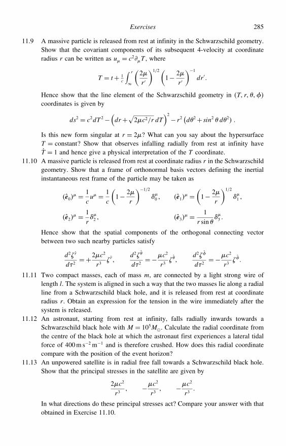
Exercises 285
11.9 A massive particle is released from rest at infinity in the Schwarzschild geometry.Show that the covariant components of its subsequent 4-velocity at coordinateradius r can be written as u = c2T , where
T = t+ 1c
∫ r
(2r ′
)1/2(1− 2
r ′
)−1dr ′
Hence show that the line element of the Schwarzschild geometry in T r
coordinates is given by
ds2 = c2dT 2−(dr+√2c2/r dT
)2− r2(d2+ sin2 d2
Is this new form singular at r = 2? What can you say about the hypersurfaceT = constant? Show that observes infalling radially from rest at infinity haveT = 1 and hence give a physical interpretation of the T coordinate.
11.10 A massive particle is released from rest at coordinate radius r in the Schwarzschildgeometry. Show that a frame of orthonormal basis vectors defining the inertialinstantaneous rest frame of the particle may be taken as
e0 = 1
cu = 1
c
(1− 2
r
)−1/20 e1
=(1− 2
r
)1/2
1
e2 = 1
r2 e3
= 1r sin
3
Hence show that the spatial components of the orthogonal connecting vectorbetween two such nearby particles satisfy
d2r
d2=+2c2
r3r
d2
d2=−c2
r3
d2
d2=−c2
r3
11.11 Two compact masses, each of mass m, are connected by a light strong wire oflength l. The system is aligned in such a way that the two masses lie along a radialline from a Schwarzschild black hole, and it is released from rest at coordinateradius r. Obtain an expression for the tension in the wire immediately after thesystem is released.
11.12 An astronaut, starting from rest at infinity, falls radially inwards towards aSchwarzschild black hole with M = 105M. Calculate the radial coordinate fromthe centre of the black hole at which the astronaut first experiences a lateral tidalforce of 400m s−2 m−1 and is therefore crushed. How does this radial coordinatecompare with the position of the event horizon?
11.13 An unpowered satellite is in radial free fall towards a Schwarzschild black hole.Show that the principal stresses in the satellite are given by
2c2
r3 −c2
r3 −c2
r3
In what directions do these principal stresses act? Compare your answer with thatobtained in Exercise 11.10.
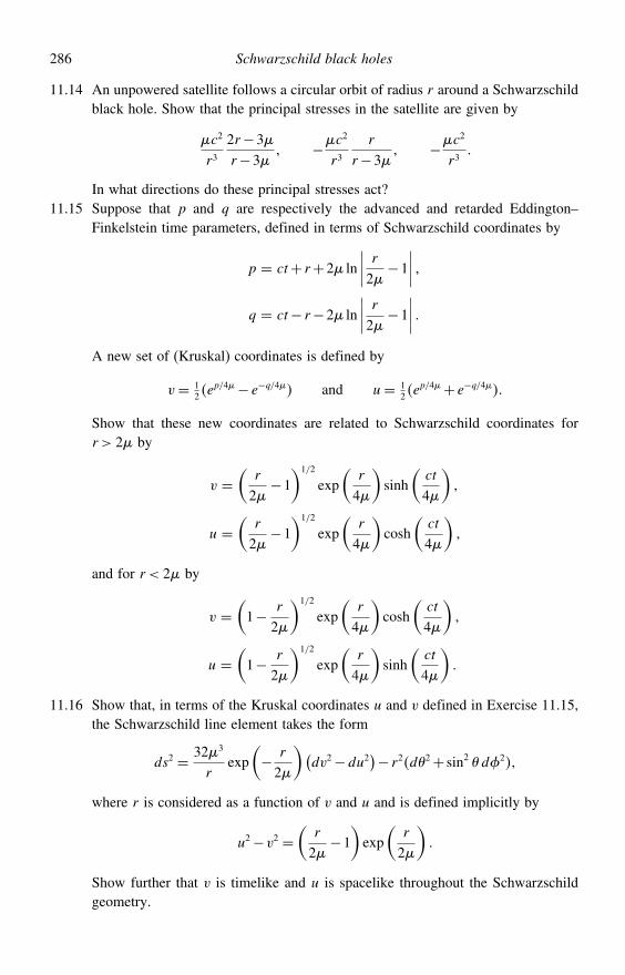
286 Schwarzschild black holes
11.14 An unpowered satellite follows a circular orbit of radius r around a Schwarzschildblack hole. Show that the principal stresses in the satellite are given by
c2
r32r−3r−3
−c2
r3r
r−3 −c2
r3
In what directions do these principal stresses act?11.15 Suppose that p and q are respectively the advanced and retarded Eddington–
Finkelstein time parameters, defined in terms of Schwarzschild coordinates by
p = ct+ r+2 ln
∣∣∣∣ r2 −1
∣∣∣∣ q = ct− r−2 ln
∣∣∣∣ r2 −1
∣∣∣∣ A new set of (Kruskal) coordinates is defined by
v= 12 e
p/4− e−q/4 and u= 12 e
p/4+ e−q/4
Show that these new coordinates are related to Schwarzschild coordinates forr > 2 by
v =(
r
2−1
)1/2
exp(
r
4
)sinh
(ct
4
)
u =(
r
2−1
)1/2
exp(
r
4
)cosh
(ct
4
)
and for r < 2 by
v =(1− r
2
)1/2
exp(
r
4
)cosh
(ct
4
)
u =(1− r
2
)1/2
exp(
r
4
)sinh
(ct
4
)
11.16 Show that, in terms of the Kruskal coordinates u and v defined in Exercise 11.15,the Schwarzschild line element takes the form
ds2 = 323
rexp
(− r
2
)(dv2−du2
)− r2d2+ sin2 d2
where r is considered as a function of v and u and is defined implicitly by
u2−v2 =(
r
2−1
)exp
(r
2
)
Show further that v is timelike and u is spacelike throughout the Schwarzschildgeometry.
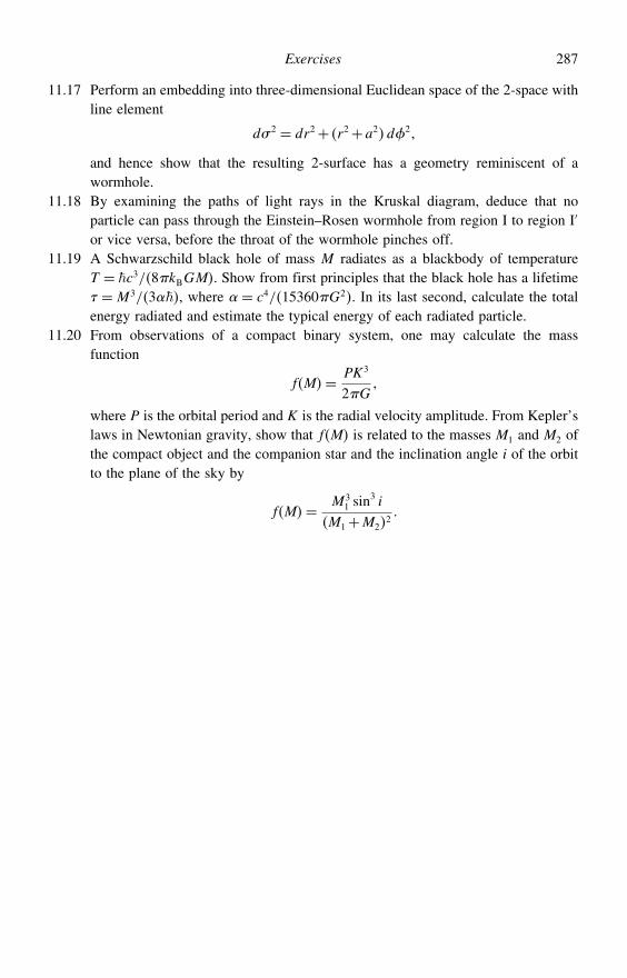
Exercises 287
11.17 Perform an embedding into three-dimensional Euclidean space of the 2-space withline element
d#2 = dr2+ r2+a2d2
and hence show that the resulting 2-surface has a geometry reminiscent of awormhole.
11.18 By examining the paths of light rays in the Kruskal diagram, deduce that noparticle can pass through the Einstein–Rosen wormhole from region I to region I′
or vice versa, before the throat of the wormhole pinches off.11.19 A Schwarzschild black hole of mass M radiates as a blackbody of temperature
T = c3/8kBGM. Show from first principles that the black hole has a lifetime =M3/3, where = c4/15360G2. In its last second, calculate the totalenergy radiated and estimate the typical energy of each radiated particle.
11.20 From observations of a compact binary system, one may calculate the massfunction
fM= PK3
2G
where P is the orbital period and K is the radial velocity amplitude. From Kepler’slaws in Newtonian gravity, show that fM is related to the masses M1 and M2 ofthe compact object and the companion star and the inclination angle i of the orbitto the plane of the sky by
fM= M31 sin
3 i
M1+M22
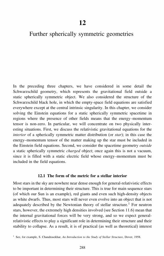
12
Further spherically symmetric geometries
In the preceding three chapters, we have considered in some detail theSchwarzschild geometry, which represents the gravitational field outside astatic spherically symmetric object. We also considered the structure of theSchwarzschild black hole, in which the empty-space field equations are satisfiedeverywhere except at the central intrinsic singularity. In this chapter, we considersolving the Einstein equations for a static spherically symmetric spacetime inregions where the presence of other fields means that the energy–momentumtensor is non-zero. In particular, we will concentrate on two physically inter-esting situations. First, we discuss the relativistic gravitational equations for theinterior of a spherically symmetric matter distribution (or star); in this case theenergy–momentum tensor of the matter making up the star must be included inthe Einstein field equations. Second, we consider the spacetime geometry outsidea static spherically symmetric charged object; once again this is not a vacuum,since it is filled with a static electric field whose energy–momentum must beincluded in the field equations.
12.1 The form of the metric for a stellar interior
Most stars in the sky are nowhere near dense enough for general-relativistic effectsto be important in determining their structure. This is true for main sequence stars(of which our Sun is an example), red giants and even such high-density objectsas white dwarfs. Thus, most stars will never even evolve into an object that is notadequately described by the Newtonian theory of stellar structure.1 For neutronstars, however, the extremely high densities involved (see Section 11.6) mean thatthe internal gravitational forces will be very strong, and so we expect general-relativistic effects to play a significant role in determining their structure and theirstability to collapse. As a result, it is of practical (as well as theoretical) interest
1 See, for example, S. Chandrasekhar, An Introduction to the Study of Stellar Structure, Dover, 1958.
288
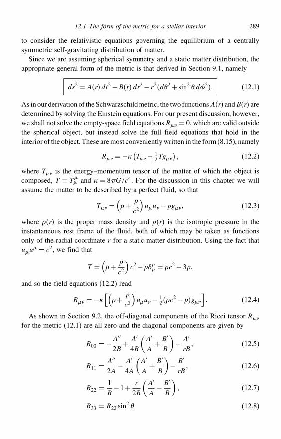
12.1 The form of the metric for a stellar interior 289
to consider the relativistic equations governing the equilibrium of a centrallysymmetric self-gravitating distribution of matter.
Since we are assuming spherical symmetry and a static matter distribution, theappropriate general form of the metric is that derived in Section 9.1, namely
ds2 = Ardt2−Brdr2− r2d2+ sin2 d2 (12.1)
As in our derivation of the Schwarzschildmetric, the two functionsAr andBr aredetermined by solving the Einstein equations. For our present discussion, however,we shall not solve the empty-space field equationsR = 0, which are valid outsidethe spherical object, but instead solve the full field equations that hold in theinterior of the object. These aremost convenientlywritten in the form (8.15), namely
R =−&(T− 1
2Tg) (12.2)
where T is the energy–momentum tensor of the matter of which the object iscomposed, T ≡ T
and & = 8G/c4. For the discussion in this chapter we will
assume the matter to be described by a perfect fluid, so that
T =(+ p
c2
)uu−pg (12.3)
where r is the proper mass density and pr is the isotropic pressure in theinstantaneous rest frame of the fluid, both of which may be taken as functionsonly of the radial coordinate r for a static matter distribution. Using the fact thatuu
= c2, we find that
T =(+ p
c2
)c2−p = c2−3p
and so the field equations (12.2) read
R =−&[(+ p
c2
)uu− 1
2c2−pg
] (12.4)
As shown in Section 9.2, the off-diagonal components of the Ricci tensor R
for the metric (12.1) are all zero and the diagonal components are given by
R00 = −A′′
2B+ A′
4B
(A′
A+ B′
B
)− A′
rB (12.5)
R11 =A′′
2A− A′
4A
(A′
A+ B′
B
)− B′
rB (12.6)
R22 =1B−1+ r
2B
(A′
A− B′
B
) (12.7)
R33 = R22 sin2 (12.8)
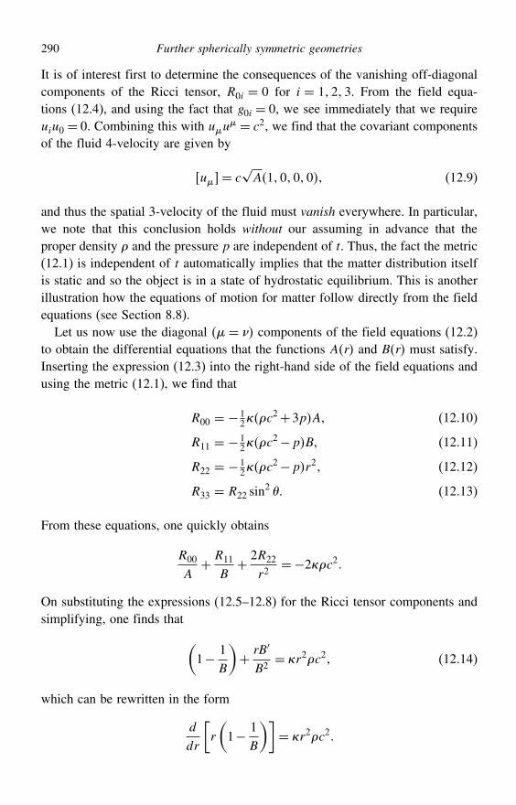
290 Further spherically symmetric geometries
It is of interest first to determine the consequences of the vanishing off-diagonalcomponents of the Ricci tensor, R0i = 0 for i = 123. From the field equa-tions (12.4), and using the fact that g0i = 0, we see immediately that we requireuiu0 = 0. Combining this with uu
= c2, we find that the covariant componentsof the fluid 4-velocity are given by
u= c√A1000 (12.9)
and thus the spatial 3-velocity of the fluid must vanish everywhere. In particular,we note that this conclusion holds without our assuming in advance that theproper density and the pressure p are independent of t. Thus, the fact the metric(12.1) is independent of t automatically implies that the matter distribution itselfis static and so the object is in a state of hydrostatic equilibrium. This is anotherillustration how the equations of motion for matter follow directly from the fieldequations (see Section 8.8).
Let us now use the diagonal = components of the field equations (12.2)to obtain the differential equations that the functions Ar and Br must satisfy.Inserting the expression (12.3) into the right-hand side of the field equations andusing the metric (12.1), we find that
R00 = − 12&c
2+3pA (12.10)
R11 = − 12&c
2−pB (12.11)
R22 = − 12&c
2−pr2 (12.12)
R33 = R22 sin2 (12.13)
From these equations, one quickly obtains
R00
A+ R11
B+ 2R22
r2=−2&c2
On substituting the expressions (12.5–12.8) for the Ricci tensor components andsimplifying, one finds that (
1− 1B
)+ rB′
B2= &r2c2 (12.14)
which can be rewritten in the form
d
dr
[r
(1− 1
B
)]= &r2c2
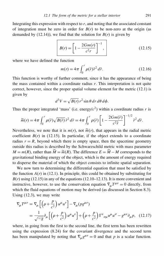
12.1 The form of the metric for a stellar interior 291
Integrating this expression with respect to r, and noting that the associated constantof integration must be zero in order for Br to be non-zero at the origin (asdemanded by (12.14)), we find that the solution for Br is given by
Br=[1− 2Gmr
c2r
]−1 (12.15)
where we have defined the function
mr= 4∫ r
0rr2 dr (12.16)
This function is worthy of further comment, since it has the appearance of beingthe mass contained within a coordinate radius r. This interpretation is not quitecorrect, however, since the proper spatial volume element for the metric (12.1) isgiven by
d3V =√Br r2 sin dr dd
Thus the proper integrated ‘mass’ (i.e. energy/c2) within a coordinate radius r is
mr= 4∫ r
0r
√Br r2 dr = 4
∫ r
0r
[1− 2Gmr
c2r
]−1/2r2 dr
Nevertheless, we note that it is mr, not mr, that appears in the radial metriccoefficient Br in (12.15). In particular, if the object extends to a coordinateradius r = R, beyond which there is empty space, then the spacetime geometryoutside this radius is described by the Schwarzschild metric with mass parameterM =mR, rather than M = mR. The difference E = M−M corresponds to thegravitational binding energy of the object, which is the amount of energy requiredto disperse the material of which the object consists to infinite spatial separation.
We now turn to determining the differential equation that must be satisfied bythe function Ar in (12.1). In principle, this could be obtained by substituting forBr using (12.15) in any of the equations (12.10–12.13). It is more convenient andinstructive, however, to use the conservation equation T
= 0 directly, fromwhich the fluid equations of motion may be derived (as discussed in Section 8.3).Using (12.3), we may write
T =
[(+ p
c2
)uu
]−pg
= 1√−g [(+ p
c2
)uu
]+(+ p
c2
)
#uu# −gp (12.17)
where, in going from the first to the second line, the first term has been rewrittenusing the expression (8.24) for the covariant divergence and the second termhas been manipulated by noting that g
= 0 and that p is a scalar function.
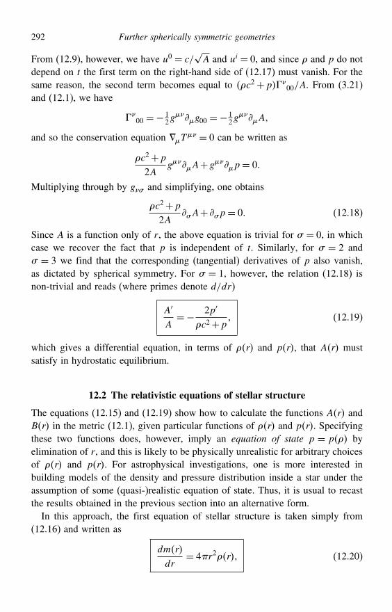
292 Further spherically symmetric geometries
From (12.9), however, we have u0 = c/√A and ui = 0, and since and p do not
depend on t the first term on the right-hand side of (12.17) must vanish. For thesame reason, the second term becomes equal to c2+p
00/A. From (3.21)and (12.1), we have
00 =− 1
2gg00 =− 1
2gA
and so the conservation equation T = 0 can be written as
c2+p
2AgA+gp= 0
Multiplying through by g# and simplifying, one obtains
c2+p
2A#A+ #p= 0 (12.18)
Since A is a function only of r, the above equation is trivial for # = 0, in whichcase we recover the fact that p is independent of t. Similarly, for # = 2 and# = 3 we find that the corresponding (tangential) derivatives of p also vanish,as dictated by spherical symmetry. For # = 1, however, the relation (12.18) isnon-trivial and reads (where primes denote d/dr)
A′
A=− 2p′
c2+p (12.19)
which gives a differential equation, in terms of r and pr, that Ar mustsatisfy in hydrostatic equilibrium.
12.2 The relativistic equations of stellar structure
The equations (12.15) and (12.19) show how to calculate the functions Ar andBr in the metric (12.1), given particular functions of r and pr. Specifyingthese two functions does, however, imply an equation of state p = p byelimination of r , and this is likely to be physically unrealistic for arbitrary choicesof r and pr. For astrophysical investigations, one is more interested inbuilding models of the density and pressure distribution inside a star under theassumption of some (quasi-)realistic equation of state. Thus, it is usual to recastthe results obtained in the previous section into an alternative form.
In this approach, the first equation of stellar structure is taken simply from(12.16) and written as
dmr
dr= 4r2r (12.20)
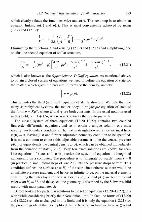
12.2 The relativistic equations of stellar structure 293
which clearly relates the functions mr and r. The next step is to obtain anequation linking mr and pr. This is most conveniently achieved by using(12.7) and (12.12):
1B−1+ r
2B
(A′
A− B′
B
)=−1
2&c2−pr2
Eliminating the functions A and B using (12.19) and (12.15) and simplifying, oneobtains the second equation of stellar structure,
dp
dr=− 1
r2c2+p
[4Gc4
pr3+ Gmr
c2
][1− 2Gmr
c2r
]−1 (12.21)
which is also known as the Oppenheimer–Volkoff equation. As mentioned above,to obtain a closed system of equations we need to define the equation of state forthe matter, which gives the pressure in terms of the density, namely
p= p (12.22)
This provides the third (and final) equation of stellar structure. We note that, formany astrophysical systems, the matter obeys a polytropic equation of state ofthe form p= K , where K and are both constants. In the usual notation usedin this field, = 1+1/n, where n is known as the polytropic index.
The closed system of three equations (12.20–12.22) contains two coupledfirst-order differential equations, and so to obtain a unique solution one mustspecify two boundary conditions. The first is straightforward, since we must havem0= 0, leaving just one further adjustable boundary condition to be specified.It is most common to choose this adjustable parameter to be the central pressurep0, or equivalently the central density 0, which can be obtained immediatelyfrom the equation of state (12.22). Very few exact solutions are known for real-istic equations of state, and so in practice the system of equations is integratednumerically on a computer. The procedure is to ‘integrate outwards’ from r = 0(in practice in small radial steps of size r) until the pressure drops to zero. Thiscondition defines the surface r = R of the star, since otherwise there would bean infinite pressure gradient, and hence an infinite force, on the material elementsconstituting the outer layer of the star. For r > Rr and pr are both zero andmr=mR=M , and the spacetime geometry is described by the Schwarzschildmetric with mass parameter M .
Before looking for particular solutions to the set of equations (12.20–12.22), it isworthwhile considering briefly their Newtonian limit. In fact, the forms of (12.20)and (12.22) remain unchanged in this limit, and it is only the equation (12.21) forthe pressure gradient that is simplified. In the Newtonian limit we have p and

294 Further spherically symmetric geometries
therefore 4r3p mc2. Moreover, we require the metric (12.1) to be close toMinkowski, and so we require 2Gm/c2r 1. Thus, the Oppenheimer–Volkoffequation reduces to
dp
dr=−Gmrr
r2 (12.23)
which is simply the Newtonian equation for hydrostatic equilibrium. Comparing(12.23) with (12.21), we see that all the relativistic effects serve to steepen thepressure gradient relative to the Newtonian case. Thus, for an object to remainin hydrostatic equilibrium, the fluid of which it consists must experience strongerinternal forces when general-relativistic effects are taken into account.
12.3 The Schwarzschild constant-density interior solution
The simplest analytic interior solution for a relativistic star is obtained by makingthe assumption that, throughout the star,
= constant
which constitutes an equation of state. There is no physical justification for thisassumption, but it is on the borderline of being realistic. It corresponds to anultra-stiff equation of state that represents an incompressible fluid. Consequently,the speed of sound in the fluid, which is proportional to dp/d1/2, is infinite(which is clearly not allowed relativistically). Nevertheless, it is believed that theinteriors of dense neutron stars are of nearly uniform density, and so this simplecase is of some practical interest.
Equation (12.20) immediately integrates to give
mr=
43r
3 for r ≤ R43R
3 ≡M for r > R(12.24)
where R is the radius of the star, as yet undetermined, andM is the mass parameterfor the Schwarzschild metric describing the spacetime geometry outside the star.Moreover, the Oppenheimer–Volkoff equation (12.21) becomes
dp
dr=−4G
3c4rc2+pc2+3p
(1− 8G
3c2r2
)−1
This equation is separable and we may write∫ pr
p0
dp
c2+ pc2+3p=−4G
3c4
∫ r
0
r dr
1−8Gr2/3c2
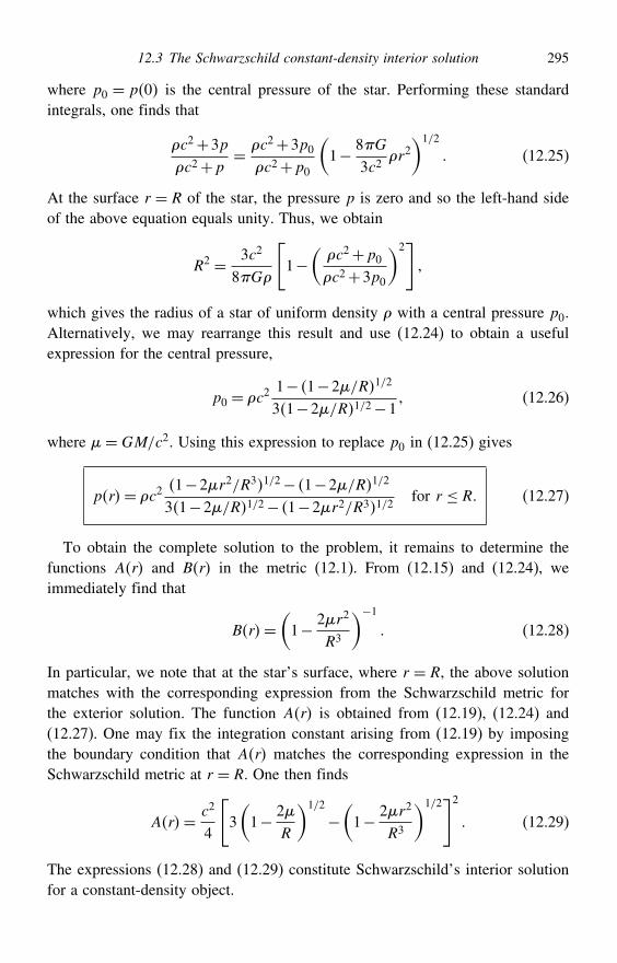
12.3 The Schwarzschild constant-density interior solution 295
where p0 = p0 is the central pressure of the star. Performing these standardintegrals, one finds that
c2+3pc2+p
= c2+3p0c2+p0
(1− 8G
3c2r2
)1/2
(12.25)
At the surface r = R of the star, the pressure p is zero and so the left-hand sideof the above equation equals unity. Thus, we obtain
R2 = 3c2
8G
[1−
(c2+p0c2+3p0
)2]
which gives the radius of a star of uniform density with a central pressure p0.Alternatively, we may rearrange this result and use (12.24) to obtain a usefulexpression for the central pressure,
p0 = c21− 1−2/R1/2
31−2/R1/2−1 (12.26)
where =GM/c2. Using this expression to replace p0 in (12.25) gives
pr= c21−2r2/R31/2− 1−2/R1/2
31−2/R1/2− 1−2r2/R31/2for r ≤ R (12.27)
To obtain the complete solution to the problem, it remains to determine thefunctions Ar and Br in the metric (12.1). From (12.15) and (12.24), weimmediately find that
Br=(1− 2r2
R3
)−1 (12.28)
In particular, we note that at the star’s surface, where r = R, the above solutionmatches with the corresponding expression from the Schwarzschild metric forthe exterior solution. The function Ar is obtained from (12.19), (12.24) and(12.27). One may fix the integration constant arising from (12.19) by imposingthe boundary condition that Ar matches the corresponding expression in theSchwarzschild metric at r = R. One then finds
Ar= c2
4
[3(1− 2
R
)1/2
−(1− 2r2
R3
)1/2]2
(12.29)
The expressions (12.28) and (12.29) constitute Schwarzschild’s interior solutionfor a constant-density object.
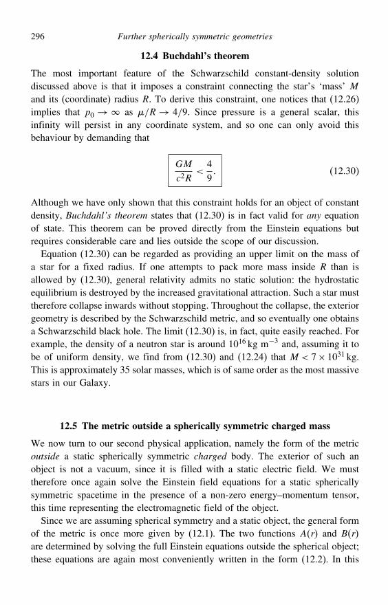
296 Further spherically symmetric geometries
12.4 Buchdahl’s theorem
The most important feature of the Schwarzschild constant-density solutiondiscussed above is that it imposes a constraint connecting the star’s ‘mass’ Mand its (coordinate) radius R. To derive this constraint, one notices that (12.26)implies that p0 → as /R→ 4/9. Since pressure is a general scalar, thisinfinity will persist in any coordinate system, and so one can only avoid thisbehaviour by demanding that
GM
c2R<
49 (12.30)
Although we have only shown that this constraint holds for an object of constantdensity, Buchdahl’s theorem states that (12.30) is in fact valid for any equationof state. This theorem can be proved directly from the Einstein equations butrequires considerable care and lies outside the scope of our discussion.
Equation (12.30) can be regarded as providing an upper limit on the mass ofa star for a fixed radius. If one attempts to pack more mass inside R than isallowed by (12.30), general relativity admits no static solution: the hydrostaticequilibrium is destroyed by the increased gravitational attraction. Such a star musttherefore collapse inwards without stopping. Throughout the collapse, the exteriorgeometry is described by the Schwarzschild metric, and so eventually one obtainsa Schwarzschild black hole. The limit (12.30) is, in fact, quite easily reached. Forexample, the density of a neutron star is around 1016 kg m−3 and, assuming it tobe of uniform density, we find from (12.30) and (12.24) that M < 7× 1031 kg.This is approximately 35 solar masses, which is of same order as the most massivestars in our Galaxy.
12.5 The metric outside a spherically symmetric charged mass
We now turn to our second physical application, namely the form of the metricoutside a static spherically symmetric charged body. The exterior of such anobject is not a vacuum, since it is filled with a static electric field. We musttherefore once again solve the Einstein field equations for a static sphericallysymmetric spacetime in the presence of a non-zero energy–momentum tensor,this time representing the electromagnetic field of the object.
Since we are assuming spherical symmetry and a static object, the general formof the metric is once more given by (12.1). The two functions Ar and Br
are determined by solving the full Einstein equations outside the spherical object;these equations are again most conveniently written in the form (12.2). In this
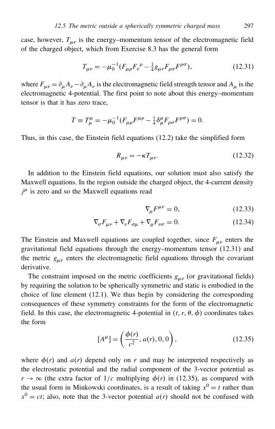
12.5 The metric outside a spherically symmetric charged mass 297
case, however, T is the energy–momentum tensor of the electromagnetic fieldof the charged object, which from Exercise 8.3 has the general form
T =−−10 FF− 1
4gF#F# (12.31)
where F = A−A is the electromagnetic field strength tensor andA is theelectromagnetic 4-potential. The first point to note about this energy–momentumtensor is that it has zero trace,
T ≡ T =−−10 FF
− 14
F#F
#= 0
Thus, in this case, the Einstein field equations (12.2) take the simplified form
R =−&T (12.32)
In addition to the Einstein field equations, our solution must also satisfy theMaxwell equations. In the region outside the charged object, the 4-current densityj is zero and so the Maxwell equations read
F = 0 (12.33)
#F+F#+F# = 0 (12.34)
The Einstein and Maxwell equations are coupled together, since F enters thegravitational field equations through the energy–momentum tensor (12.31) andthe metric g enters the electromagnetic field equations through the covariantderivative.
The constraint imposed on the metric coefficients g (or gravitational fields)by requiring the solution to be spherically symmetric and static is embodied in thechoice of line element (12.1). We thus begin by considering the correspondingconsequences of these symmetry constraints for the form of the electromagneticfield. In this case, the electromagnetic 4-potential in t r coordinates takesthe form
A=(r
c2 ar00
) (12.35)
where r and ar depend only on r and may be interpreted respectively asthe electrostatic potential and the radial component of the 3-vector potential asr → (the extra factor of 1/c multiplying r in (12.35), as compared withthe usual form in Minkowski coordinates, is a result of taking x0 = t rather thanx0 = ct; also, note that the 3-vector potential ar should not be confused with
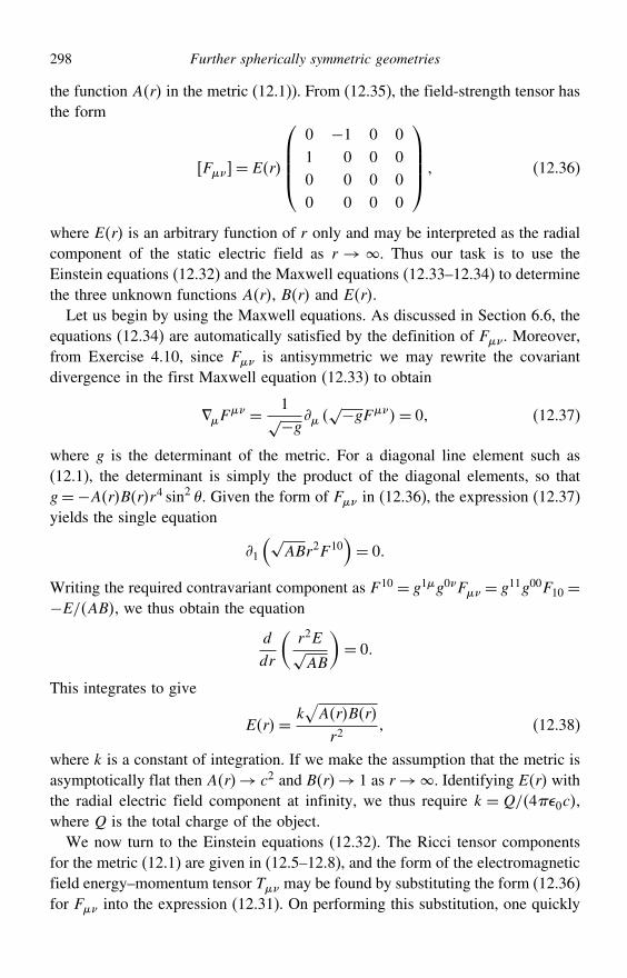
298 Further spherically symmetric geometries
the function Ar in the metric (12.1)). From (12.35), the field-strength tensor hasthe form
F= Er
⎛⎜⎜⎜⎝0 −1 0 01 0 0 00 0 0 00 0 0 0
⎞⎟⎟⎟⎠ (12.36)
where Er is an arbitrary function of r only and may be interpreted as the radialcomponent of the static electric field as r →. Thus our task is to use theEinstein equations (12.32) and the Maxwell equations (12.33–12.34) to determinethe three unknown functions Ar, Br and Er.
Let us begin by using the Maxwell equations. As discussed in Section 6.6, theequations (12.34) are automatically satisfied by the definition of F. Moreover,from Exercise 4.10, since F is antisymmetric we may rewrite the covariantdivergence in the first Maxwell equation (12.33) to obtain
F = 1√−g
√−gF= 0 (12.37)
where g is the determinant of the metric. For a diagonal line element such as(12.1), the determinant is simply the product of the diagonal elements, so thatg =−ArBrr4 sin2 . Given the form of F in (12.36), the expression (12.37)yields the single equation
1
(√ABr2F 10
)= 0
Writing the required contravariant component as F 10 = g1g0F = g11g00F10 =−E/AB, we thus obtain the equation
d
dr
(r2E√AB
)= 0
This integrates to give
Er= k√ArBr
r2 (12.38)
where k is a constant of integration. If we make the assumption that the metric isasymptotically flat then Ar→ c2 and Br→ 1 as r→. Identifying Er withthe radial electric field component at infinity, we thus require k = Q/40c,where Q is the total charge of the object.
We now turn to the Einstein equations (12.32). The Ricci tensor componentsfor the metric (12.1) are given in (12.5–12.8), and the form of the electromagneticfield energy–momentum tensor T may be found by substituting the form (12.36)for F into the expression (12.31). On performing this substitution, one quickly
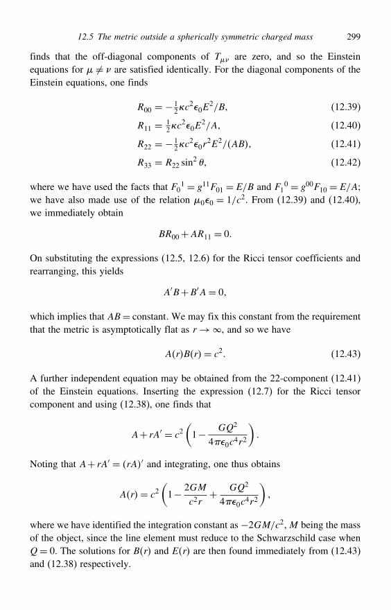
12.5 The metric outside a spherically symmetric charged mass 299
finds that the off-diagonal components of T are zero, and so the Einsteinequations for = are satisfied identically. For the diagonal components of theEinstein equations, one finds
R00 = − 12&c
20E2/B (12.39)
R11 = 12&c
20E2/A (12.40)
R22 = − 12&c
20r2E2/AB (12.41)
R33 = R22 sin2 (12.42)
where we have used the facts that F01 = g11F01 = E/B and F1
0 = g00F10 = E/A;we have also made use of the relation 00 = 1/c2. From (12.39) and (12.40),we immediately obtain
BR00+AR11 = 0
On substituting the expressions (12.5, 12.6) for the Ricci tensor coefficients andrearranging, this yields
A′B+B′A= 0
which implies that AB= constant. We may fix this constant from the requirementthat the metric is asymptotically flat as r→, and so we have
ArBr= c2 (12.43)
A further independent equation may be obtained from the 22-component (12.41)of the Einstein equations. Inserting the expression (12.7) for the Ricci tensorcomponent and using (12.38), one finds that
A+ rA′ = c2(1− GQ2
40c4r2
)
Noting that A+ rA′ = rA′ and integrating, one thus obtains
Ar= c2(1− 2GM
c2r+ GQ2
40c4r2
)
where we have identified the integration constant as −2GM/c2,M being the massof the object, since the line element must reduce to the Schwarzschild case whenQ= 0. The solutions for Br and Er are then found immediately from (12.43)and (12.38) respectively.
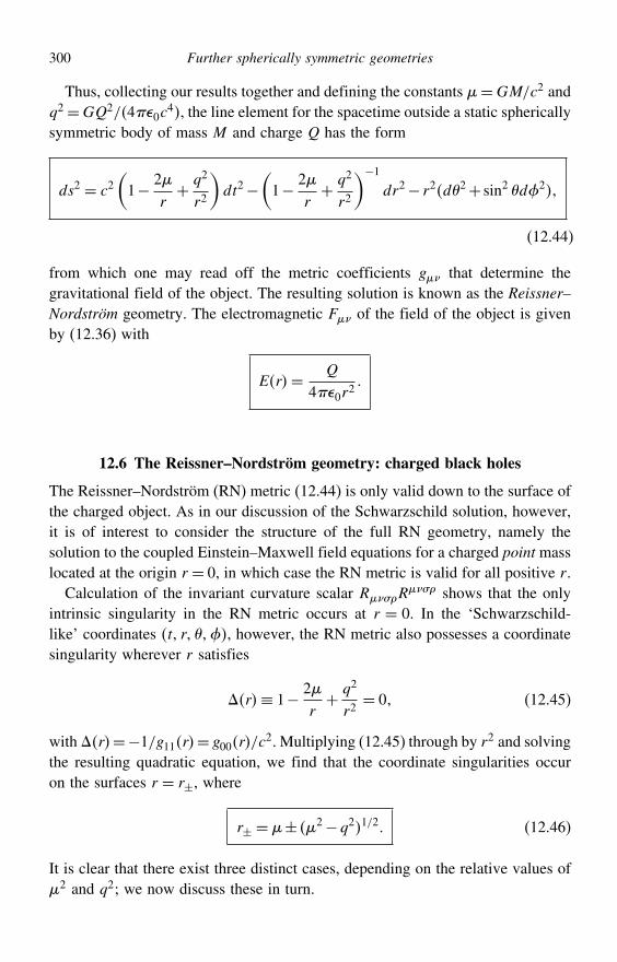
300 Further spherically symmetric geometries
Thus, collecting our results together and defining the constants =GM/c2 andq2=GQ2/40c
4, the line element for the spacetime outside a static sphericallysymmetric body of mass M and charge Q has the form
ds2 = c2(1− 2
r+ q2
r2
)dt2−
(1− 2
r+ q2
r2
)−1dr2− r2d2+ sin2 d2
(12.44)
from which one may read off the metric coefficients g that determine thegravitational field of the object. The resulting solution is known as the Reissner–Nordström geometry. The electromagnetic F of the field of the object is givenby (12.36) with
Er= Q
40r2
12.6 The Reissner–Nordström geometry: charged black holes
The Reissner–Nordström (RN) metric (12.44) is only valid down to the surface ofthe charged object. As in our discussion of the Schwarzschild solution, however,it is of interest to consider the structure of the full RN geometry, namely thesolution to the coupled Einstein–Maxwell field equations for a charged point masslocated at the origin r = 0, in which case the RN metric is valid for all positive r.
Calculation of the invariant curvature scalar R#R# shows that the only
intrinsic singularity in the RN metric occurs at r = 0. In the ‘Schwarzschild-like’ coordinates t r , however, the RN metric also possesses a coordinatesingularity wherever r satisfies
r≡ 1− 2r+ q2
r2= 0 (12.45)
with r=−1/g11r= g00r/c2. Multiplying (12.45) through by r2 and solving
the resulting quadratic equation, we find that the coordinate singularities occuron the surfaces r = r±, where
r± = ± 2−q21/2 (12.46)
It is clear that there exist three distinct cases, depending on the relative values of2 and q2; we now discuss these in turn.
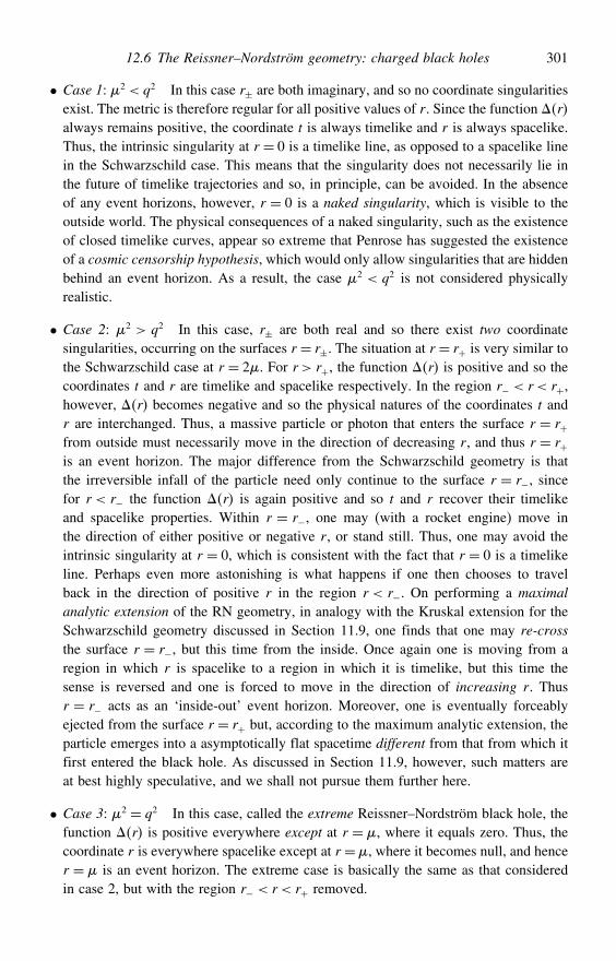
12.6 The Reissner–Nordström geometry: charged black holes 301
• Case 1: 2 < q2 In this case r± are both imaginary, and so no coordinate singularitiesexist. The metric is therefore regular for all positive values of r. Since the function ralways remains positive, the coordinate t is always timelike and r is always spacelike.Thus, the intrinsic singularity at r = 0 is a timelike line, as opposed to a spacelike linein the Schwarzschild case. This means that the singularity does not necessarily lie inthe future of timelike trajectories and so, in principle, can be avoided. In the absenceof any event horizons, however, r = 0 is a naked singularity, which is visible to theoutside world. The physical consequences of a naked singularity, such as the existenceof closed timelike curves, appear so extreme that Penrose has suggested the existenceof a cosmic censorship hypothesis, which would only allow singularities that are hiddenbehind an event horizon. As a result, the case 2 < q2 is not considered physicallyrealistic.
• Case 2: 2 > q2 In this case, r± are both real and so there exist two coordinatesingularities, occurring on the surfaces r = r±. The situation at r = r+ is very similar tothe Schwarzschild case at r = 2. For r > r+, the function r is positive and so thecoordinates t and r are timelike and spacelike respectively. In the region r− < r < r+,however, r becomes negative and so the physical natures of the coordinates t andr are interchanged. Thus, a massive particle or photon that enters the surface r = r+from outside must necessarily move in the direction of decreasing r, and thus r = r+is an event horizon. The major difference from the Schwarzschild geometry is thatthe irreversible infall of the particle need only continue to the surface r = r−, sincefor r < r− the function r is again positive and so t and r recover their timelikeand spacelike properties. Within r = r−, one may (with a rocket engine) move inthe direction of either positive or negative r, or stand still. Thus, one may avoid theintrinsic singularity at r = 0, which is consistent with the fact that r = 0 is a timelikeline. Perhaps even more astonishing is what happens if one then chooses to travelback in the direction of positive r in the region r < r−. On performing a maximalanalytic extension of the RN geometry, in analogy with the Kruskal extension for theSchwarzschild geometry discussed in Section 11.9, one finds that one may re-crossthe surface r = r−, but this time from the inside. Once again one is moving from aregion in which r is spacelike to a region in which it is timelike, but this time thesense is reversed and one is forced to move in the direction of increasing r. Thusr = r− acts as an ‘inside-out’ event horizon. Moreover, one is eventually forceablyejected from the surface r = r+ but, according to the maximum analytic extension, theparticle emerges into a asymptotically flat spacetime different from that from which itfirst entered the black hole. As discussed in Section 11.9, however, such matters areat best highly speculative, and we shall not pursue them further here.
• Case 3: 2 = q2 In this case, called the extreme Reissner–Nordström black hole, thefunction r is positive everywhere except at r = , where it equals zero. Thus, thecoordinate r is everywhere spacelike except at r =, where it becomes null, and hencer = is an event horizon. The extreme case is basically the same as that consideredin case 2, but with the region r− < r < r+ removed.
302 Further spherically symmetric geometries
We may illustrate the properties of the RN spacetime in more detail by consideringthe paths of photons and massive particles in the geometry, which we now go onto discuss. Since the case 2 >q2 is the most physically reasonable RN spacetime,we shall restrict our discussion to this situation.
12.7 Radial photon trajectories in the RN geometry
Let us begin by investigating the paths of radially incoming and outgoing photonsin the RN metric for the case 2 > q2. Since ds = d = d = 0 for a radiallymoving photon, we have immediately from (12.44) that
dt
dr=±1
c=(1− 2
r+ q2
r2
)−1=±1
c
r2
r− r−r− r+ (12.47)
where, in the second equality, we have used the result (12.46); the plus signcorresponds to an outgoing photon and the minus sign to an incoming photon. Onintegrating, we obtain
ct = r− r2−r+− r−
ln
∣∣∣∣ rr− −1
∣∣∣∣+ r2+r+− r−
ln
∣∣∣∣ rr+ −1
∣∣∣∣+ constant outgoing
ct = −r+ r2−r+− r−
ln
∣∣∣∣ rr− −1
∣∣∣∣− r2+r+− r−
ln
∣∣∣∣ rr+ −1
∣∣∣∣+ constant ingoing
We will concentrate in particular on the ingoing radial photons. To develop abetter description of infalling particles in general, we may construct the equivalentof the advanced Eddington–Finkelstein coordinates derived for the Schwarzschildmetric in Section 11.5. Once again this coordinate system is based on radiallyinfalling photons, and the trick is to use the integration constant as the newcoordinate, which we denote by p. As before, p is a null coordinate and it is moreconvenient to work instead with the timelike coordinate t′ defined by ct′ = p− r.Thus, we have
ct′ = ct− r2−r+− r−
ln
∣∣∣∣ rr− −1
∣∣∣∣+ r2+r+− r−
ln
∣∣∣∣ rr+ −1
∣∣∣∣ (12.48)
On differentiating, or from (12.47) directly, one obtains
c dt′ = dp−dr = c dt+[
1r
−1]dr (12.49)
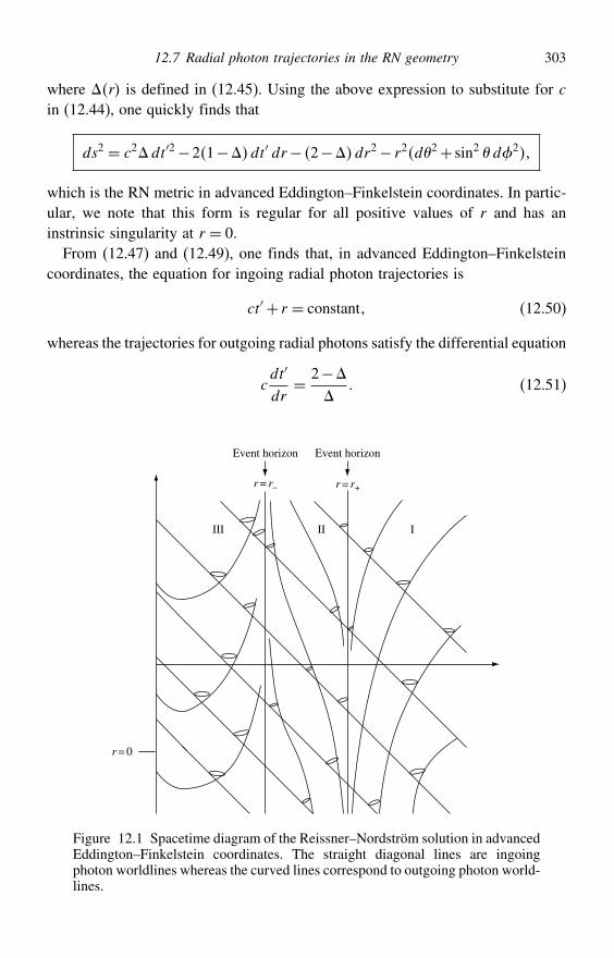
12.7 Radial photon trajectories in the RN geometry 303
where r is defined in (12.45). Using the above expression to substitute for cin (12.44), one quickly finds that
ds2 = c2dt′2−21−dt′ dr− 2−dr2− r2d2+ sin2 d2
which is the RN metric in advanced Eddington–Finkelstein coordinates. In partic-ular, we note that this form is regular for all positive values of r and has aninstrinsic singularity at r = 0.
From (12.47) and (12.49), one finds that, in advanced Eddington–Finkelsteincoordinates, the equation for ingoing radial photon trajectories is
ct′ + r = constant (12.50)
whereas the trajectories for outgoing radial photons satisfy the differential equation
cdt′
dr= 2−
(12.51)
II I
r = r–
III
r = r+
Event horizon Event horizon
r = 0
Figure 12.1 Spacetime diagram of the Reissner–Nordström solution in advancedEddington–Finkelstein coordinates. The straight diagonal lines are ingoingphoton worldlines whereas the curved lines correspond to outgoing photon world-lines.
304 Further spherically symmetric geometries
We may use these equations to determine the light-cone structure of the RN metricin these coordinates. For ingoing radial photons, the trajectories (12.50) are simplystraight lines at 45 in a spacetime diagram. For outgoing radial photons, (12.51)gives the gradient of the trajectory at any point in the spacetime diagram, and soone may sketch these without solving (12.51) explicitly. This resulting spacetimediagram is shown in Figure 12.1. It is worth noting that the light-cone structuredepicted confirms the nature of the event horizon at r = r+. Moreover, the light-cones remain tilted over in the region r− < r < r+, indicating that any particlefalling into this region must move inwards until it reaches r = r−. Once in theregion r < r−, the lightcones are no longer tilted and so particles need not fall intothe singularity r = 0. As was the case in Section 11.5 for the Schwarzschild metric,however, this spacetime diagram may be somewhat misleading. For an outward-moving particle in the region r < r−, Figure 12.1 suggests that it can only reachr = r− asymptotically, but by peforming an analytic extension of the RN solutionone can show that the particle can cross the surface r = r− in finite proper time.
12.8 Radial massive particle trajectories in the RN geometry
We now consider the trajectories of radially moving massive particles for thecase 2 > q2. To simplify our discussion, we will assume that the particles areelectrically neutral. In this case, the particles will follow geodesics. In the moregeneral case of an electrically charged particle, one must also take into accountthe Lorenz force on the particle produced by the electromagnetic field of the blackhole. The equation of motion for the particle is then given by (6.13).
For a radially moving particle, the 4-velocity has the form
u= u0 u100= t r00
where the dots denote differentiation with respect to the proper time of theparticle. The geodesic equations of motion, obeyed by neutral particles in the RNmetric, are most conveniently written in the form (3.56):
u# = 12#gu
u
Since the metric coefficients in the RN line element (12.44) do not depend on t,we immediately obtain
u0 = g00 t = constant
The radial equation of motion may then be obtained using the normalisationcondition gu
u = c2, which gives
g00u02+g11u
12 = c2
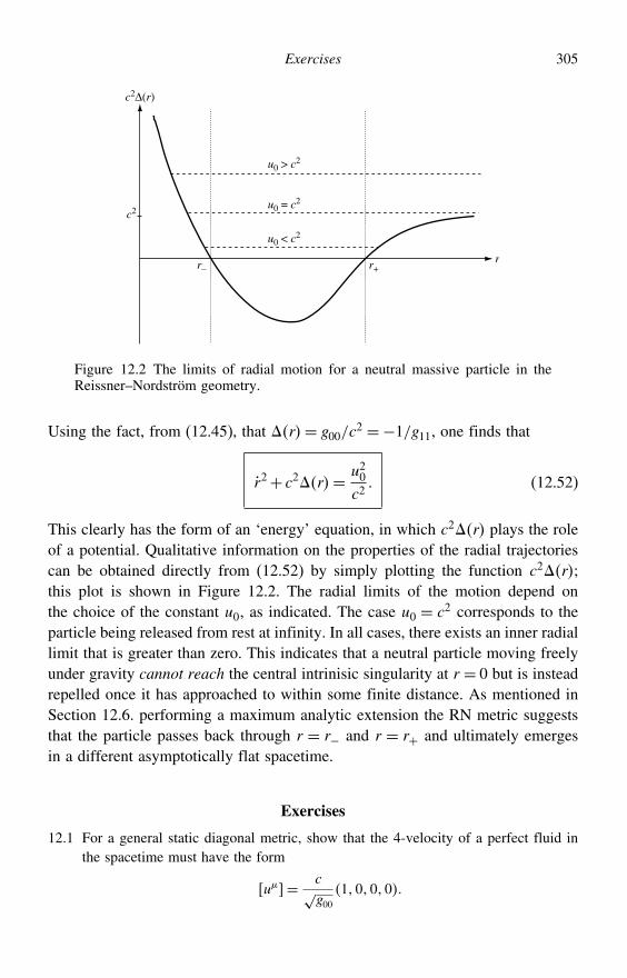
Exercises 305
r
u0 > c2
u0 = c2
u0 < c2
r+r–
c2
c2∆(r)
Figure 12.2 The limits of radial motion for a neutral massive particle in theReissner–Nordström geometry.
Using the fact, from (12.45), that r= g00/c2 =−1/g11, one finds that
r2+ c2r= u20c2 (12.52)
This clearly has the form of an ‘energy’ equation, in which c2r plays the roleof a potential. Qualitative information on the properties of the radial trajectoriescan be obtained directly from (12.52) by simply plotting the function c2r;this plot is shown in Figure 12.2. The radial limits of the motion depend onthe choice of the constant u0, as indicated. The case u0 = c2 corresponds to theparticle being released from rest at infinity. In all cases, there exists an inner radiallimit that is greater than zero. This indicates that a neutral particle moving freelyunder gravity cannot reach the central intrinisic singularity at r = 0 but is insteadrepelled once it has approached to within some finite distance. As mentioned inSection 12.6. performing a maximum analytic extension the RN metric suggeststhat the particle passes back through r = r− and r = r+ and ultimately emergesin a different asymptotically flat spacetime.
Exercises
12.1 For a general static diagonal metric, show that the 4-velocity of a perfect fluid inthe spacetime must have the form
u= c√g00
1000
306 Further spherically symmetric geometries
12.2 Calculate the gravitational binding energy E= M−M of a spherical star of constantdensity and coordinate radius R. Compare your answer with the correspondingNewtonian result and interpret your findings physically.
12.3 Derive the Oppenheimer–Volkoff equation from the Einstein equations for a staticspherically symmetric perfect-fluid distribution, and show that it reduces to thestandard equation for hydrostatic equilibrium in the Newtonian limit.
12.4 In Newtonian gravity, show directly that the equation for hydrostatic equilibrium is
dpr
dr=−Gmrr
r2
12.5 Show that, in the Newtonian limit, the equation before (12.15) reduces to
d%r
dr= Gmr
r
where %r is the Newtonian gravitational potential.12.6 For a spherical star of uniform density and central pressure p0, verify that the
Oppenheimer–Volkoff equation requires pr to satisfy
c2+3prc2+pr
= c2+3p0
c2+p0
(1− 8G
3c2r2
)1/2
and hence show that
pr= c21−2r2/R31/2− 1−2/R1/2
31−2/R1/2− 1−2r2/R31/2
where R is the coordinate radius of the star.12.7 In Newtonian gravity, obtain the expression for pr for a spherical star of uniform
density , central pressure p0 and radius R. Compare your result with that obtainedin Exercise 12.6.
12.8 Show that, for a spherical star of uniform density ,
R2 <c2
3Gand M2 <
16c6
243G3
If a photon is emitted from the star’s surface and received by a stationary observerat infinity, show that the observed redshift must obey the constraint z < 2. Showalso, however, that the observed redshift for a photon emitted from the star’s centrecan be arbitrarily large.
12.9 For a spherical star of uniform density , show that in order for the star not to liewithin its own Schwarzschild radius, one requires
M2 <3c6
32G3
Compare this limit with that derived in Exercise 12.8.
Exercises 307
12.10 For a spherical uniform-density star of mass M and coordinate radius R, show thatthe line element of spatial sections with t = constant can be written in the form
d#2 = Rc2
2GM
[d2+ sin2 d2+ sin2 d2
]
12.11 Consider a static infinitely long cylindrical configuration of matter that is invariantto translations and Lorentz boosts along the axis of symmetry (a cosmic string).Adopting ‘cylindrical polar’ coordinates ct r z, show that a self-consistentsolution to the Einstein field equations may be obtained if the stress-energy tensorfor the matter is of the form
T= diagc200−c2such that there is a negative pressure (or tension) along the string, and the lineelement is of the form
ds2 = c2 dt2−dr2−Brd2−dz2
where Br satisfies
B′′
2B− B′2
4B2=−&c2
Show further that br=√Br satisfies b′′ = −&c2b.Hint: You may find your answers to Exercises 8.9, 9.28 and 9.29 useful.
12.12 Suppose that the matter distribution in a cosmic string has a uniform density acrossthe string, such that
r=0 for r ≤ r0
0 for r > r0
By demanding that g→−r2 as r→ 0, so that the spacetime geometry is regularon the axis of the string, show that the line element for r ≤ r0 is
ds2 = c2 dt2−dr2−(sinrr
)2
d2−dz2
where = √&0c2. By demanding that g and its derivative with respect to r
are both continuous at r = r0, show that the line element for r > r0 is
ds2 = c2 dt2−dr2−[sinr0r
+ r− r0 cosr0
]2d2−dz2
For the interesting case in which r0 1, show that for r r0 the line elementtakes the form
ds2 = c2 dt2−dr2−(1− 8G
c2
)r2 d2−dz2
308 Further spherically symmetric geometries
where = r200 is the ‘mass per unit length’ of the string. Interpret this lineelement physically.
12.13 Show that the electromagnetic field tensor outside a static spherically symmetriccharged matter distribution has the form
F= Er
⎛⎜⎜⎜⎝0 −1 0 0
1 0 0 0
0 0 0 0
0 0 0 0
⎞⎟⎟⎟⎠
where Er is some arbitrary function. Hence show that, if the line element outsidethe matter distribution has the form
ds2 = Ardt2−Brdr2− r2d2+ sin2 d2
the energy–momentum tensor of the electromagnetic field in this region is given by
T=12c20E
2 diag
(1B− 1
Ar2E2
ABr2E2 sin2
AB
)
12.14 Calculate the invariant curvature scalar R#R# for the Reissner–Nordström
geometry and hence show that the only intrinsic singularity occurs at r = 0.12.15 Show that the worldlines of radially moving photons in the Reissner–Nordström
geometry are given by
ct = r− r2−r+− r−
ln
∣∣∣∣ rr− −1
∣∣∣∣+ r2+r+− r−
ln
∣∣∣∣ rr+ −1
∣∣∣∣+ constant outgoing
ct =−r+ r2−r+− r−
ln
∣∣∣∣ rr− −1
∣∣∣∣− r2+r+− r−
ln
∣∣∣∣ rr+ −1
∣∣∣∣+ constant ingoing
12.16 Show that, by introducing the advanced Eddington–Finkelstein timelike coordinate
ct′ = ct− r2−r+− r−
ln
∣∣∣∣ rr− −1
∣∣∣∣+ r2+r+− r−
ln
∣∣∣∣ rr+ −1
∣∣∣∣ the Reissner–Nordström line element takes the form
ds2 = c2dt′2−21−dt′ dr− 2−dr2− r2d2+ sin2 d2
where ≡ r = 1− 2/r+q2/r2. Hence show that the worldlines of radiallymoving photons in advanced Eddington–Finkelstein coordinates are given by
ct′ + r = constant incoming cdt′
dr= 2−
outgoing
What is the significance, if any, of the fact that c dt′/dr = 0 at r = 2 foroutgoing radially moving photons?
Exercises 309
12.17 For a particle of mass m and charge e in geodesic motion in the Reissner–Nordström geometry, show that the quantity
k=m
(1− 2
r+ q2
r2
)dt
d+ eq
r
is conserved, and interpret this result physically.12.18 An observer is in a circular orbit of coordinate radius r = R in the Reissner–
Nordström geometry. Find the components of the magnetic field measured by theobserver.
13
The Kerr geometry
The Schwarzschild solution describes the spacetime geometry outside a spheri-cally symmetric massive object, characterised only by its mass M . In the previouschapter we derived further spherically symmetric solutions. Most real astrophys-ical objects, however, are rotating. In this case, a spherically symmetric solutioncannot apply because the rotation axis of the object defines a special direction, sodestroying the isotropy of the solution. For this reason, in general relativity it is notpossible to find a coordinate system that reduces the spacetime geometry outsidea rotating (uncharged) body to the Schwarzschild geometry. The non-linear fieldequations couple the source to the exterior geometry. Moreover, a rotating bodyis characterised not only by its mass M but also by its angular momentum J , andso we would expect the corresponding spacetime metric to depend upon thesetwo parameters.
We now consider how to derive the metric describing the spacetime geometryoutside a rotating body. Since the mathematical complexity in this case is fargreater than that encountered in deriving the Schwarzschild metric (or the otherspherically symmetric geometries discussed in the previous chapter), we shallcontent ourselves with just an outline of how the solution may be obtained.
13.1 The general stationary axisymmetric metric
In our derivation of the Schwarzschild solution, we began by constructing thegeneral form of the static isotropic metric. We are now interested in deriving thespacetime geometry outside a steadily rotating massive body. Thus we begin byconstructing the general form of the stationary axisymmetric metric.
For the description of such a spacetime, it is convenient to introduce thetimelike coordinate t= x0 and the azimuthal angle = x3 about the axis ofsymmetry. The stationary and axisymmetric character of the spacetime requires
310
13.1 The general stationary axisymmetric metric 311
that the metric coefficients g be independent of t and , so that
g = gx1 x2
where x1 and x2 are the two remaining spacelike coordinates.Besides stationarity and axisymmetry, we shall also require that the line element
is invariant to simultaneous inversion of the coordinates t and , i.e. the trans-formations
t→−t and →−The physical meaning of this additional requirement is that the source of thegravitational field, whatever it may be, has motions that are purely rotationalabout the axis of symmetry, i.e. we are considering the spacetime associated witha rotating body. This assumed invariance requires that
g01 = g02 = g13 = g23 = 0
since the corresponding terms in the line element would change sign under thesimultaneous inversion of t and . Therefore, under the assumptions made thusfar, the line element must have the form
ds2 = g00 dt2+2g03 dt d+g33 d
2+ [g11dx12+2g12 dx1 dx2+g22dx
22]
(13.1)
We note that, since the metric coefficients g are functions only of x1 andx2, the expression in square brackets in (13.1) can be considered as a separatetwo-dimensional submanifold. A further reduction in the form of the metric canthus be achieved by using the fact that any two-dimensional (pseudo-)Riemannianmanifold is conformally flat, i.e. it is always possible to find a coordinate systemin which the metric takes the form
gab =2xab (13.2)
where2x is an arbitrary function of the coordinates and ab= diag±1±1;the signs depend on the signature of the manifold. We proved this result inAppendix 11C. Thus, taking advantage of this fact, and writing the result in waysuggestive of a rotating body, we can express the line element (13.1) in the form
ds2 = Adt2−Bd−dt2−C[dx12+ dx22
] (13.3)
where ABC and are arbitrary functions of the spacelike coordinates x1 and x2.For definiteness, let us denote the coordinates x1 and x2 by r and respectively.
For our axisymmetric metric, these coordinates are not so readily associated withany geometrical meaning. Nevertheless, in order that they can be chosen later tobe as similar as possible to the spherically symmetric r and , it is useful to allow
312 The Kerr geometry
some extra freedom in the metric by not demanding that the metric coefficientsg22 and g33 be identical. Thus, from now on we will work with the metric
ds2 = Adt2−Bd−dt2−C dr2−Dd2 (13.4)
where ABCD and are arbitrary functions of the spacelike coordinates r
and but we have the freedom to relate C and D in such a way so that thephysical meanings of r and are as close as possible to the spherically symmetriccase. The functions in (13.4) are related to the metric coefficients g by
gtt = A−B2 gt = B g =−B grr =−C g =−Dwhere, from now on, we use coordinate names rather than numbers to denote thecomponents. Note that =−gt/g and, if the body is not rotating, we can set = 0 since in this case we would require that the metric is invariant under thesingle transformation t→−t and consequently gt = 0.
For later convenience, let us also calculate the contravariant components g ofthe metric corresponding to the line element (13.4). The only off-diagonal termsinvolve t and , and so immediately we have
grr =−1/C g =−1/DTo find the remaining contravariant components, we must invert the matrix
G=(gtt gtgt g
)⇒ G−1 = 1
G
(g −gt−gt gtt
)
where the determinant G = gttg− gt2 =−AB. Thus
gtt = g
G =1A gt =−gt
G =
A g = gtt
G =B2−A
AB (13.5)
Shortly we will show that a metric of the form (13.4) can indeed be made tosatisfy the empty-space field equations R = 0 by suitable choice of the functionsABCD and . Before specialising to any particular solution, however, weinvestigate three particularly interesting generic properties of such spacetimes:the dragging of inertial frames and the existence of stationary limit surfaces andevent horizons.
13.2 The dragging of inertial frames
The presence of gt = 0 in the metric (13.4) introduces qualitatively new effectsinto particle trajectories. Since g is independent of , the covariant componentp of a particle’s 4-momentum is still conserved along its geodesic. Indeed
13.2 The dragging of inertial frames 313
p =−L, where L is the component of angular momentum of the particle alongthe rotation axis, which is conserved (note the minus sign, which also occurred inthe Schwarzschild case discussed in Chapter 9). This conservation law is a directconsequence of the axisymmetry of the spacetime. Note, however, that the totalangular momentum of a particle is not a conserved quantity, since the spacetimeis not spherically symmetric about any point.
The corresponding contravariant component p of the particle’s 4-momentumis given by
p = gp = gtpt+gp
and similarly the contravariant time component of the 4-momentum is
pt = gtp = gttpt+gtp
Let is now consider a particle (or photon) with zero angular momentum, so thatp = 0 along its geodesic. Using the definition of the 4-momentum, for either amassive particle or a photon we have
pt ∝ dt
d#and p ∝ d
d#
where # is an affine parameter along the geodesic and the constants of propor-tionality in each case are equal. Thus the particle’s trajectory is such that
d
dt= p
pt= gt
gtt= r
This equation defines what we mean by : it is the coordinate angular velocityof a zero-angular-momentum particle.
We shall find the explicit form for for the Kerr geometry later, but it isclear that this effect is present in any metric for which gt = 0, which in turnhappens whenever the source of the gravitational field is rotating. So we have theremarkable result that a particle dropped ‘straight in’ from infinity p = 0 is‘dragged’ just by the influence of gravity so that it acquires an angular velocityin the same sense as that of the source of the metric. This effect weakens withdistance (roughly as ∼1/r3 for the Kerr metric) and makes the angular momentumof the source measurable in practice.
The effect is called the dragging of inertial frames. Remember that inertialframes are defined as those in which free-falling test bodies are stationary or movealong straight lines at constant speed. Consider the freely falling particle discussedabove. At any spatial point r , in order for the particle to be at rest in some(inertial) frame the frame must be moving with an angular speedr . Any otherinertial frame is then related to this instantaneous rest frame by a Lorentz transfor-mation. Thus the inertial frames are ‘dragged’ by the rotating source. A schematic
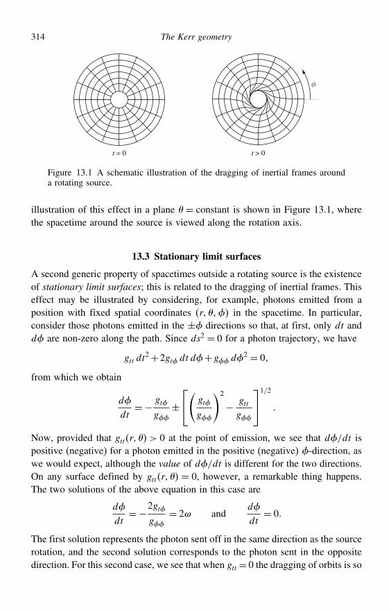
314 The Kerr geometry
φ
t = 0 t > 0
Figure 13.1 A schematic illustration of the dragging of inertial frames arounda rotating source.
illustration of this effect in a plane = constant is shown in Figure 13.1, wherethe spacetime around the source is viewed along the rotation axis.
13.3 Stationary limit surfaces
A second generic property of spacetimes outside a rotating source is the existenceof stationary limit surfaces; this is related to the dragging of inertial frames. Thiseffect may be illustrated by considering, for example, photons emitted from aposition with fixed spatial coordinates r in the spacetime. In particular,consider those photons emitted in the ± directions so that, at first, only dt andd are non-zero along the path. Since ds2 = 0 for a photon trajectory, we have
gtt dt2+2gt dt d+g d
2 = 0
from which we obtain
d
dt=− gt
g±⎡⎣( gt
g
)2
− gttg
⎤⎦1/2
Now, provided that gttr > 0 at the point of emission, we see that d/dt ispositive (negative) for a photon emitted in the positive (negative) -direction, aswe would expect, although the value of d/dt is different for the two directions.On any surface defined by gttr = 0, however, a remarkable thing happens.The two solutions of the above equation in this case are
d
dt=−2gt
g= 2 and
d
dt= 0
The first solution represents the photon sent off in the same direction as the sourcerotation, and the second solution corresponds to the photon sent in the oppositedirection. For this second case, we see that when gtt = 0 the dragging of orbits is so
13.4 Event horizons 315
severe that the photon initially does not move at all! Clearly, any massive particle,which must move more slowly than a photon, will therefore have to rotate withthe source, even if it has an angular momentum arbitrarily large in the oppositesense. Any surface defined by gttr = 0 is called a stationary limit surface.Inside the surface, where gtt < 0, no particle can remain at fixed r but mustinstead rotate around the source in the same sense as the source’s rotation. Thisis consistent with our discussion of the Schwarzschild metric, for which gtt = 0occurs at r = 2, within which no particle can remain at fixed spatial coordinates.
The fact that a particle (or observer) cannot remain at a fixed r inside astationary limit surface, where gtt < 0, may also be shown directly by consideringthe 4-velocity of an observer at fixed r , which is given by
u= ut000 (13.6)
We require, however, that u · u = gttut2 = c2, but this cannot be satisfied if
gtt < 0, hence showing that a 4-velocity of the form (13.6) is not possible in sucha region.
Any surface defined by gtt = 0 is also physically interesting in another way. InAppendix 9A, we presented a general approach to the calculation of gravitationalredshifts. In particular, we showed that, for an emitter E and receiver R with fixedspatial coordinates in a stationary spacetime (i.e. one for which tg = 0), thegravitational frequency shift of a photon is, quite generally,
RE=[gttA
gttB
]1/2
where A is the event at which the photon is emitted and B the event at whichit is received. Thus, we see that if the photon is emitted from a point with fixedspatial coordinates, then R → 0 in the limit gtt → 0, so that the photon suffersan infinite redshift. Thus a surface defined by gttr = 0 is also often calledan infinite redshift surface. This is again consistent with our discussion of theSchwarzschild metric, for which the surface r = 2 (where gtt = 0) is indeed aninfinite redshift surface.
13.4 Event horizons
In the Schwarzschild metric, the surface r = 2 is both a surface of infiniteredshift and an event horizon, but in our more general axisymmetric spacetimethese surfaces need not coincide. In general, as we shall see below, the definingproperty of an event horizon is that it is a null 3-surface, i.e. a surface whosenormal at every point is a null vector.
316 The Kerr geometry
Before discussing the particular case of a stationary axisymmetric spacetime,let us briefly consider null 3-surfaces in general. Suppose that such a surface isdefined by the equation
fx= 0
The normal to the surface is directed along the 4-gradient n = f = f
(remembering that f is a scalar quantity), and for a null surface we have
gnn = 0 (13.7)
This last property means that the direction of the normal lies in the surfaceitself; along the surface df = n dx
= 0, and this equation is satisfied when thedirections of the 4-vectors dx and n coincide. In this same direction, from theproperty (13.7) we see that the element of length in the 3-surface is ds = 0. Inother words, along this direction the 3-surface is tangent, at any given point, tothe lightcone at that point. Thus, the lightcone at each point of a null 3-surface(say, in the future direction) lies entirely on one side of the surface and is tangentto the 3-surface at that point. This means that the (future-directed) worldline of aparticle or photon can cross a null 3-surface in only one direction, and hence thelatter forms an event horizon.
In a stationary axisymmetric spacetime the equation of the surface must takethe form
fr = 0
Moreover, the condition that the surface is null means that
gff= 0
which, for a metric of the form (13.4), reduces to
grrrf2+gf
2 = 0 (13.8)
This is therefore the general condition for a surface fr to be an event horizon.We may, however, choose our coordinates r and in such a way that we can
write the equation of the surface as fr= 0, i.e. as a function of r alone. In thiscase, the condition (13.8) reduces to
grrrf2 = 0
from which we see that an event horizon occurs when grr = 0, or equivalentlygrr = . This is consistent with our analysis of the Schwarzschild metric, forwhich grr = at r = 2.
13.5 The Kerr metric 317
13.5 The Kerr metric
So far our discussion has been limited to using symmetry arguments to restrictthe possible form of the stationary axisymmetric line element, which we assumedto be
ds2 = gtt dt2+2gt dt d+g d
2+grr dr2+g d
2 (13.9)
or, equivalently,
ds2 = Adt2−Bd−dt2−C dr2−Dd2 (13.10)
where the arbitrary functions in either form depend only on r and . As we haveseen, the general form of this line element leads to some interesting new physicalphenomena in such spacetimes. Nevertheless, we must now verify that such aline element does indeed satisfy Einstein’s gravitational field equations and thusobtain explicit forms for the metric functions appearing in ds2.
The general approach to performing this calculation is the same as that used inderiving the Schwarzschild metric. We first calculate the connection coefficients
# for the metric (13.9) or (13.10) and then use these coefficients to obtainexpressions for the components R of the Ricci tensor in terms of the unknownfunctions in the line element. Since we are again interested in the spacetimegeometry outside the rotating matter distribution, we must then solve the empty-space field equations
R = 0
Although this process is conceptually straightforward, it is algebraically verycomplicated, and the full calculation is extremely lengthy.1
In fact, one finds that the Einstein equations alone are insufficient to deter-mine all the unknown functions uniquely. This should not come as a surprisesince the requirement of axisymmetry is far less restrictive than that of sphericalsymmetry, used in the derivation of the Schwarzschild geometry. Although weare envisaging a ‘compact’ rotating body, such as a star or planet, the generalform of the metric (13.10) would also be valid outside a rotating ‘extended’axisymmetric body, such as a rotating cosmic string. To obtain the Kerr metric,we must therefore impose some additional conditions on the solution. It tran-spires that if we demand that the spacetime geometry tends to the Minkowskiform as r → and that somewhere there exists a smooth closed convex eventhorizon outside which the geometry is non-singular, then the solution is unique.
1 For a full derivation, see (for example) S. Chandrasekhar, The Mathematical Theory of Black Holes, OxfordUniversity Press, 1983.
318 The Kerr geometry
In this case, in terms of our ‘Schwarzschild-like’ coordinates t r , the lineelement for the Kerr geometry takes the form
ds2 = c2(1− 2r
2
)dt2+ 4acr sin2
2dt d− 2
dr2−2 d2
−(r2+a2+ 2ra2 sin2
2
)sin2 d2
(13.11)
where and a are constants and we have introduced the functions 2 and ,defined by
2 = r2+a2 cos2 = r2−2r+a2
This standard expression for ds2 is known as the Boyer–Lindquist form andt r as Boyer–Lindquist coordinates. The dedicated student may wish toverify that this metric does indeed satisfy the empty-space field equations.
We can write the metric (13.11) in several other useful forms. In particular, itis common also to define the function
(2 = r2+a22−a2 sin2
and write the metric as
ds2 = −a2 sin2 2
c2 dt2+ 4ar sin2 2
c dt d
− 2
dr2−2 d2− (2 sin2
2d2
(13.12)
This form can be rearranged in a manner that is more suggestive of a rotatingobject, to give
ds2 = 2
(2c2 dt2− (2 sin2
2d−wdt2− 2
dr2−2 d2 (13.13)
where the physically meaningful function is given by = 2cra/(2.For later convenience, it is useful to calculate the covariant components g
of the Kerr metric in Boyer–Lindquist coordinates. Using our earlier calculations
13.6 Limits of the Kerr metric 319
for the general stationary axisymmetric metric, we find that grr and g are simplythe reciprocals of grr and g respectively,
grr =−
2 g =− 1
2
whereas the remaining contravariant components are given by
gtt = (2
c22 gt = 2ar
c2 g = a2 sin2 −
2 sin2
13.6 Limits of the Kerr metric
We see that the Kerr metric depends on two parameters and a, as we mightexpect for a rotating body. Moreover, in the limit a→ 0,
→ r2(1− 2
r
)
2 → r2
(2 → r4
and so any of the forms for the Kerr metric above tends to the Schwarzschildform,
ds2→ c2(1− 2
r
)dt2−
(1− 2
r
)−1dr2− r2 d2− r2 sin2 d2
Thus suggests that we should make the identification = GM/c2, where M isthe mass of the body, and also that a corresponds in some way to the angularvelocity of the body. In fact, by investigating the slow-rotation weak-field limit(see Section 13.20), one can show that the angular momentum J of the bodyabout its rotation axis is given by J =Mac.
The fact that the Kerr metric tends to the Schwarzschild metric as a→ 0 allowsus to give some geometrical meaning to the coordinates r and in the limit of aslowly rotating body. In the general case, however, r and are not the standardSchwarzschild polar coordinates. In particular, from (13.11) we see that surfacest = constant, r = constant do not have the metric of 2-spheres.
The geometrical nature of Boyer–Lindquist coordinates is elucidated further byconsidering the Kerr metric in the limit → 0, i.e. in the absence of a gravitatingmass, in which case the spacetime should be Minkowski. One quickly finds that,in this limit, the line element becomes
ds2 = c2 dt2− 2
r2+a2dr2−2 d2− r2+a2 sin2 d2
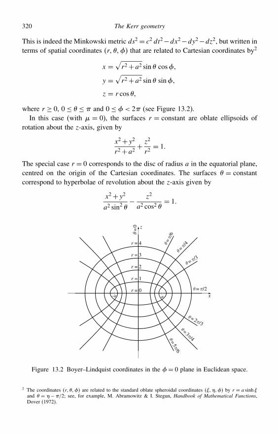
320 The Kerr geometry
This is indeed the Minkowski metric ds2= c2 dt2−dx2−dy2−dz2, but written interms of spatial coordinates r that are related to Cartesian coordinates by2
x =√r2+a2 sin cos
y =√r2+a2 sin sin
z = r cos
where r ≥ 0, 0 ≤ ≤ and 0 ≤ < 2 (see Figure 13.2).In this case (with = 0), the surfaces r = constant are oblate ellipsoids of
rotation about the z-axis, given by
x2+y2
r2+a2+ z2
r2= 1
The special case r = 0 corresponds to the disc of radius a in the equatorial plane,centred on the origin of the Cartesian coordinates. The surfaces = constantcorrespond to hyperbolae of revolution about the z-axis given by
x2+y2
a2 sin2 − z2
a2 cos2 = 1
θ = 2π/3
θ = π/3
θ=π/6
θ=π/4
θ=3π/4
z
θ = π/2x
θ=5π/6
–a a
r = 4
r = 3
r = 2
r = 1
r = 0
θ=0
Figure 13.2 Boyer–Lindquist coordinates in the = 0 plane in Euclidean space.
2 The coordinates r are related to the standard oblate spheroidal coordinates by r = a sinh and = −/2; see, for example, M. Abramowitz & I. Stegun, Handbook of Mathematical Functions,Dover (1972).
13.7 The Kerr–Schild form of the metric 321
The asymptote for large values of r is a cone, with its vertex at the origin, thatsubtends a half-angle . The angle is the standard azimuthal angle. Clearly, inthe limit a→ 0 the coordinates r correspond to standard spherical polarcoordinates. It should be remembered, however, that the simple interpretation ofthe coordinates given above no longer holds in the general case of the Kerr metric,when = 0.
13.7 The Kerr–Schild form of the metric
The form (13.11) for the line element is not in fact the form originally discoveredby Roy Kerr in 1963. Indeed, Kerr himself followed an approach to the derivationvery different from that presented here. His original interest was in line elementsof the general form
ds2 = dx dx−ll dx
dx
where the vector l is null with respect to the Minkowski metric , i.e.
ll = 0
This form for a line element is now known as the Kerr–Schild form. Kerr showedthat a line element of this form satisfied the empty-space field equations (togetherwith our additional conditions on the solution mentioned above), provided that
= 2r3
r2+a2z2
[l] = (
crx+ay
a2+y2ry−ax
a2+y2z
r
)
where x= t x y z and r is defined implicitly in terms of x y and z by
r4− r2x2+y2+ z2−a2−a2z2 = 0 (13.14)
The corresponding form for the line element is given by
ds2 = c2 dt2−dx2−dy2−dz2− 2r3
r4+a2z2
×[c d t− r
r2+a2xdx+y dy− a
r2+a2xdy−y dx− z
rdz
]2
(13.15)
322 The Kerr geometry
It is straightforward, but lengthy, to show that the two forms (13.15) and (13.11)for the line element are identical if the two sets of coordinates are related by
c d t = c dt− 2r
dr (13.16)
x = r cos′ +a sin′ sin (13.17)
y = r sin′ −a cos′ sin (13.18)
z = r cos (13.19)
where d′ = d− a/dr.
13.8 The structure of a Kerr black hole
The Kerr metric is the solution to the empty-space field equations outside arotating massive object and so is only valid down to the surface of the object.As in our discussion of the Schwarzschild solution, however, it is of interest toconsider the structure of the full Kerr geometry as a vacuum solution to the fieldequations.
Singularities and horizons
The Kerr metric in Boyer–Lindquist coordinates is singular when = 0 and when= 0. Calculation of the invariant curvature scalar R#R
# reveals that only= 0 is an intrinsic singularity. Since
2 = r2+a2 cos2 = 0
it follows that this occurs when
r = 0 = /2
From our earlier discussion of Boyer–Lindquist coordinates, we recall that r = 0represents a disc of coordinate radius a in the equatorial plane. Moreover, thecollection of points with r = 0 and =/2 constitutes the outer edge of this disc.Thus, rather surprisingly, the singularity has the form of a ring, of coordinateradius a, lying in the equatorial plane. Similarly, using (13.14) and (13.19), wesee that, in terms of the ‘Cartesian’ coordinates t x y z, the singularity occurswhen x2+y2 = a2 and z= 0.The points where = 0 are coordinate singularities, which occur on the surfaces
r± = ± (2−a2)1/2
(13.20)
13.8 The structure of a Kerr black hole 323
As discussed above, event horizons in the Kerr metric will occur where r =constant is a null 3-surface, and this is given by the condition grr = 0 or, equiva-lently, grr =. From (13.11), we have
grr =−2
from which we see that the surfaces r = r+ and r = r−, for which = 0, arein fact event horizons. Thus, the Kerr metric has two event horizons. In theSchwarzschild limit a→ 0, these reduce to r = 2 and r = 0. The surfaces r = r±are axially symmetric, but their intrinsic geometries are not spherically symmetric.Setting r = r± and t = constant in the Kerr metric and noting from (13.20) thatr2±+a2 = 2r±, we obtain two-dimensional surfaces with the line elements
d#2 = 2± d2+
(2r±±
)2
sin2 d2 (13.21)
which do not describe the geometry of a sphere. If one embeds a 2-surface withgeometry given by (13.21) in three-dimensional Euclidean space, one obtains asurface resembling an axisymmetric ellipsoid, flattened along the rotation axis.
The existence of the outer horizon r = r+, in particular, shows that the Kerrgeometry represents a (rotating) black hole. It is a one-way surface, like r = 2in the Schwarzschild geometry. Particles and photons can cross it once, from theoutside, but not in the opposite direction. It is common practice to define threedistinct regions of a Kerr black hole, bounded by the event horizons, in which thesolution is regular: region I, r+ < r <; region II, r− < r < r+; and region III,0< r < r−.Not all values of and a correspond to a black hole, however. From (13.20),
we see that horizons (at real values of r) exist only for
a2 < 2 (13.22)
Thus the magnitude of the angular momentum J =Mac of a rotating black holeis limited by its squared mass. Moreover, if the condition (13.22) is satisfiedthen the intrinsic singularity at = 0 is contained safely within the outer horizonr = r+. An extreme Kerr black hole is one that has the limiting value a2 = 2.In this case, the event horizons r+ and r− coincide at r = . It may be thatnear-extreme Kerr black holes develop naturally in many astrophysical situations.Matter falling towards a rotating black hole forms an accretion disc that rotatesin the same sense as the hole. As matter from the disc spirals inwards and fallsinto the black hole, it carries angular momentum with it and hence increases theangular momentum of the hole. The process is limited by the fact that radiationfrom the infalling matter carries away angular momentum. Detailed calculations
324 The Kerr geometry
suggest that the limiting value is a≈ 0998, which is very close to the extremevalue.
For a2 > 2 we find that > 0 throughout, and so the Kerr metric is regulareverywhere except = 0, where there is a ring singularity. Since the horizonshave disappeared, this means that the ring singularity is visible to the outsideworld. In fact, one can show explicitly that timelike and null geodesics in theequatorial plane can start at the singularity and reach infinity, thereby makingthe singularity visible to the outside world. Such a singularity is called a nakedsingularity (as mentioned in Section 12.6) and opens up an enormous realm forsome truly wild speculation. However, Penrose’s cosmic censorship hypothesisonly allows singularities that are hidden behind an event horizon.
Stationary limit surfaces
As we showed earlier, in a general stationary axisymmetric spacetime the condi-tion gtt = 0 defines a surface that is both a stationary limit surface and a surfaceof infinite redshift. For the Kerr metric, we have
gtt = c2(1− 2r
2
)= c2
r2−2r+a2 cos2 2
so that (for a2 ≤ 2) these surfaces, S+ and S−, occur at
rS± = ± (2−a2 cos2 )1/2
The two surfaces are axisymmetric, but setting r = rS± and t = constant in theKerr metric, and noting from (13.20) that r2
S± +a2 = 2rS± +a2 sin2 , we obtaintwo-dimensional surfaces with line elements
d#2 = 2S± d2+
[2rS±2rS± +2a2 sin2
2S±
]sin2 d2 (13.23)
which again do not describe the geometry of a sphere. If one embeds a 2-surfacewith geometry given by (13.23) in three-dimensional Euclidean space then asurface resembling an axisymmetric ellipsoid, flattened along the rotation axis, isonce more obtained. In the Schwarzschild limit a→ 0, the surface S+ reduces tor = 2 and S− to r = 0. As anticipated we see that, in the Schwarzschild solution,the surfaces of infinite redshift and the event horizons coincide.
The surface S− coincides with the ring singularity in the equatorial plane.Moreover, S− lies completely within the inner horizon r = r− (except at the poles,where they touch). The surface S+ has coordinate radius 2 at the equator and,for all , it completely encloses the outer horizon r = r+ (except at the poles,where they touch), giving rise to a region between the two called the ergoregion.The structure of a Kerr black hole is illustrated in Figure 13.3.
13.8 The structure of a Kerr black hole 325
Infinite redshiftsurface S–
Event horizon r = r–
Ring singularityEvent horizon r = r+
Stationary limitsurface (infiniteredshift surface) S+
Ergosphere
z
y
Symmetry axis (θ = 0)
Figure 13.3 The structure of a Kerr black hole.
The ergoregion
The ergoregion gets its name from the Greek word ergo meaning work. Thekey property of an ergoregion (which can occur in other spacetime geometries)is that it is a region for which gtt < 0 and from which particles can escape.Clearly, the Schwarzschild geometry does not possess an ergoregion, since gtt < 0is only satisfied within its event horizon. As we will discuss in Section 13.9,Roger Penrose has shown that it is possible to extract the rotational energy ofa Kerr black hole from within the ergoregion. To assist in that discussion, it isuseful here to consider the constraints induced by the spacetime geometry on themotion of observers within the ergoregion.
Since gtt < 0 at all points within the ergoregion, an immediate consequence (asalready discussed in Section 13.3) is that an observer (even in a spaceship withan arbitrarily powerful rocket) cannot remain at a fixed r position. The4-velocity of such an observer would be given by
u= ut000 (13.24)
but the requirement that u ·u= gttut2= c2 cannot be satisfied if gtt < 0, showing
that a 4-velocity of the form (13.24) is not possible.It is possible, however, for a rocket-powered observer to remain at fixed r
and coordinates by rotating around the black hole (with respect to an observerat infinity) in the same sense as the hole’s rotation; this is an illustration of theframe-dragging phenomenon discussed in Section 13.3. The 4-velocity of such anobserver is
u= ut100 (13.25)
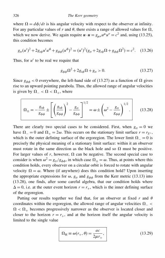
326 The Kerr geometry
where = d/dt is his angular velocity with respect to the observer at infinity.For any particular values of r and , there exists a range of allowed values for ,which we now derive. We again require u ·u= gu
u = c2 and, using (13.25),this condition becomes
gttut2+2gtu
tu+gu2 = ut2gtt+2gt+g
2= c2 (13.26)
Thus, for ut to be real we require that
g2+2gt+gtt > 0 (13.27)
Since g < 0 everywhere, the left-hand side of (13.27) as a function of givesrise to an upward pointing parabola. Thus, the allowed range of angular velocitiesis given by − <<+, where
± = −gt
g±⎡⎣( gt
g
)2
− gttg
⎤⎦1/2
= ±(2− gtt
g
)1/2
(13.28)
There are clearly two special cases to be considered. First, when gtt = 0 wehave − = 0 and + = 2. This occurs on the stationary limit surface r = rS+ ,which is the outer defining surface of the ergoregion. The lower limit − = 0 isprecisely the physical meaning of a stationary limit surface: within it an observermust rotate in the same direction as the black hole and so must be positive.For larger values of r , however, can be negative. The second special case toconsider is when 2 = gtt/g, in which case ± =. Thus, at points where thiscondition holds, every observer on a circular orbit is forced to rotate with angularvelocity = . Where (if anywhere) does this condition hold? Upon insertingthe appropriate expressions for , gtt and g from the Kerr metric (13.13) into(13.28), one finds, after some careful algebra, that our condition holds where= 0, i.e. at the outer event horizon r = r+, which is the inner defining surfaceof the ergoregion.
Putting our results together we find that, for an observer at fixed r and
coordinates within the ergoregion, the allowed range of angular velocities − <
< + becomes progressively narrower as the observer is located closer andcloser to the horizon r = r+, and at the horizon itself the angular velocity islimited to the single value
H ≡ r+ =ac
2r+ (13.29)
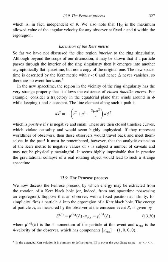
13.9 The Penrose process 327
which is, in fact, independent of . We also note that H is the maximumallowed value of the angular velocity for any observer at fixed r and within theergoregion.
Extension of the Kerr metric
So far we have not discussed the disc region interior to the ring singularity.Although beyond the scope of our discussion, it may be shown that if a particlepasses through the interior of the ring singularity then it emerges into anotherasymptotically flat spacetime, but not a copy of the original one. The new space-time is described by the Kerr metric with r < 0 and hence never vanishes, sothere are no event horizons.3
In the new spacetime, the region in the vicinity of the ring singularity has thevery strange property that it allows the existence of closed timelike curves. Forexample, consider a trajectory in the equatorial plane that winds around in
while keeping t and r constant. The line element along such a path is
ds2 =−(r2+a2+ 2a2
r
)d2
which is positive if r is negative and small. These are then closed timelike curves,which violate causality and would seem highly unphysical. If they representworldlines of observers, then these observers would travel back and meet them-selves in the past! It must be remembered, however, that the analytic extensionof the Kerr metric to negative values of r is subject a number of caveats andmay not be physically meaningful. It seems highly improbable that in practicethe gravitational collapse of a real rotating object would lead to such a strangespacetime.
13.9 The Penrose process
We now discuss the Penrose process, by which energy may be extracted fromthe rotation of a Kerr black hole (or, indeed, from any spacetime possessingan ergoregion). Suppose that an observer, with a fixed position at infinity, forsimplicity, fires a particle A into the ergoregion of a Kerr black hole. The energyof particle A, as measured by the observer at the emission event , is given by
EA = pA ·uobs = pAt (13.30)
where pA is the 4-momentum of the particle at this event and uobs is the4-velocity of the observer, which has components uobs= 1000.
3 In the extended Kerr solution it is common to define region III to cover the coordinate range −< r < r−.
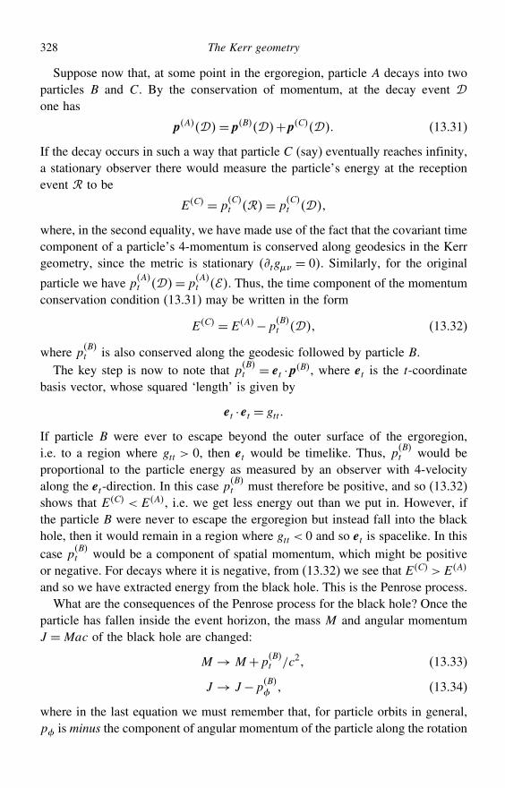
328 The Kerr geometry
Suppose now that, at some point in the ergoregion, particle A decays into twoparticles B and C. By the conservation of momentum, at the decay event one has
pA= pB+pC (13.31)
If the decay occurs in such a way that particle C (say) eventually reaches infinity,a stationary observer there would measure the particle’s energy at the receptionevent to be
EC = pCt = p
Ct
where, in the second equality, we have made use of the fact that the covariant timecomponent of a particle’s 4-momentum is conserved along geodesics in the Kerrgeometry, since the metric is stationary tg = 0. Similarly, for the original
particle we have pAt = pAt . Thus, the time component of the momentum
conservation condition (13.31) may be written in the form
EC = EA−pBt (13.32)
where pBt is also conserved along the geodesic followed by particle B.The key step is now to note that pBt = et · pB, where et is the t-coordinate
basis vector, whose squared ‘length’ is given by
et · et = gtt
If particle B were ever to escape beyond the outer surface of the ergoregion,i.e. to a region where gtt > 0, then et would be timelike. Thus, pBt would beproportional to the particle energy as measured by an observer with 4-velocityalong the et-direction. In this case pBt must therefore be positive, and so (13.32)shows that EC < EA, i.e. we get less energy out than we put in. However, ifthe particle B were never to escape the ergoregion but instead fall into the blackhole, then it would remain in a region where gtt < 0 and so et is spacelike. In thiscase p
Bt would be a component of spatial momentum, which might be positive
or negative. For decays where it is negative, from (13.32) we see that EC > EA
and so we have extracted energy from the black hole. This is the Penrose process.What are the consequences of the Penrose process for the black hole? Once the
particle has fallen inside the event horizon, the mass M and angular momentumJ =Mac of the black hole are changed:
M → M+pBt /c2 (13.33)
J → J −pB (13.34)
where in the last equation we must remember that, for particle orbits in general,p is minus the component of angular momentum of the particle along the rotation
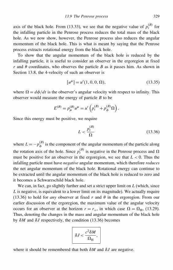
13.9 The Penrose process 329
axis of the black hole. From (13.33), we see that the negative value of pBt forthe infalling particle in the Penrose process reduces the total mass of the blackhole. As we now show, however, the Penrose process also reduces the angularmomentum of the black hole. This is what is meant by saying that the Penroseprocess extracts rotational energy from the black hole.
To show that the angular momentum of the black hole is reduced by theinfalling particle, it is useful to consider an observer in the ergoregion at fixedr and coordinates, who observes the particle B as it passes him. As shown inSection 13.8, the 4-velocity of such an observer is
u= ut100 (13.35)
where = d/dt is the observer’s angular velocity with respect to infinity. Thisobserver would measure the energy of particle B to be
EB = pB u = ut(pBt +p
B
)
Since this energy must be positive, we require
L <pBt
(13.36)
where L=−pB is the component of the angular momentum of the particle along
the rotation axis of the hole. Since pBt is negative in the Penrose process and
must be positive for an observer in the ergoregion, we see that L < 0. Thus theinfalling particle must have negative angular momentum, which therefore reducesthe net angular momentum of the black hole. Rotational energy can continue tobe extracted until the angular momentum of the black hole is reduced to zero andit becomes a Schwarzschild black hole.
We can, in fact, go slightly further and set a strict upper limit on L (which, sinceL is negative, is equivalent to a lower limit on its magnitude). We actually require(13.36) to hold for any observer at fixed r and in the ergoregion. From ourearlier discussion of the ergoregion, the maximum value of the angular velocityoccurs for an observer at the horizon r = r+, in which case = H, (13.29).Thus, denoting the changes in the mass and angular momentum of the black holeby M and J respectively, the condition (13.36) becomes
J <c2M
H
where it should be remembered that both M and J are negative.
330 The Kerr geometry
13.10 Geodesics in the equatorial plane
As one might expect, the general equations for non-null and null geodesics in theKerr geometry are much less tractable than in the Schwarzschild case, and particletrajectories exhibit complicated behaviour. For example, in general the trajectoryof a massive particle or photon is not constrained to lie in a plane. This is a directconsequence of the fact that the spacetime is not spherically symmetric and so, ingeneral, the angular momentum of a test particle is not conserved. Since the Kerrgeometry is stationary and axisymmetric, the conserved quantities along particletrajectories are pt and p. The latter corresponds to the conservation of only thecomponent of angular momentum along the rotation axis. Nevertheless, since themetric is reflection-symmetric through the equatorial plane, particles for whichp = 0, i.e. which are initially in the equatorial plane, will always have p = 0 andso the trajectory remains in this plane. We shall therefore confine our attention tothis simpler special case.
Setting = /2 in the Kerr metric (13.11), we obtain
ds2 = c2(1− 2
r
)dt2+ 4ac
rdt d− r2
dr2−
(r2+a2+ 2a2
r
)d2
(13.37)from which the covariant metric components g in the equatorial plane canbe read off. Following the method described in Section 13.1, the correspondingcontravariant metric components are found to be
gtt = 1c2
(r2+a2+ 2a2
r
) gt = 2a
cr
grr =−
r2 g =− 1
(1− 2
r
)
From (13.37) one can immediately write down the corresponding ‘Lagrangian’ = gx
x. In the interests of notational simplicity, for a massive particle weshall take the particle to have unit rest mass and for a photon we shall choosean appropriate affine parameter along the null geodesic such that, in both cases,p = x. One may obtain the geodesic equations by writing down the appropriateEuler–Lagrange equations. It is quicker, however, simply to use the fact that pt andp are conserved along geodesics (since the metric does not depend explicitly ont and ), which leads immediately to the first integrals of the t- and - equations.These are given by
pt = gttt+gt= c2(1− 2
r
)t+ 2ac
r= kc2 (13.38)
p = gtt+g=2acr
t−(r2+a2+ 2a2
r
)=−h (13.39)
13.10 Geodesics in the equatorial plane 331
where we have defined the constants k and h so that in the Schwarzschild limita→ 0 they coincide with the constants introduced in Chapter 9. This pair ofsimultaneous equations for t and is straightforwardly solved to give
t = 1
[(r2+a2+ 2a2
r
)k− 2a
crh
]
= 1
[2acr
k+(1− 2
r
)h
]
(13.40)
Instead of using the complicated Euler–Lagrange equation for r, we may usethe first integral provided by the invariant length of the 4-momentum p. Sincethe covariant components of p are particularly simple, the most convenient formto use is gpp = 2, where 2 = c2 for a massive particle and 2 = 0 for aphoton.4 Since p = 0 this gives
gttpt2+2gtptp+gp
2+grrpr2 = 2 (13.41)
where, for the moment, it is simpler not to write out the contravariant metriccomponents in full. By substituting pt = kc2 and p = −h into (13.41) andremembering that pr = grr r and grr = 1/grr , we may then obtain the ‘energy’equation for equatorial trajectories, which gives r in terms of only r and a set ofconstants. This yields
r2 = grr2−gttc4k2+2gtc2kh−gh2 (13.42)
At this stage, we may (if we wish) substitute the explicit forms for the contravariantmetric coefficients to obtain
r2 = c2k2− 2+ 22r
+ a2c2k2− 2−h2
r2+ 2h−ack2
r3 (13.43)
In the limit a→ 0, the energy equation reduces to those derived in Chapter 9for massive-particle 2 = c2 and photon 2 = 0 orbits in the Schwarzschildgeometry.
Since we are restricting our attention to the equatorial plane, we need notconsider the Euler–Lagrange equation for , since it will not yield an independentequation of motion. Thus, equations (13.40) and (13.43) completely determinethe null and non-null geodesics in the equatorial plane for given values of theconstants k and h.
4 The device of working in terms of 2 allows one to calculate the null and non-null geodesic equationssimultaneously; one simply sets 2 to the appropriate value at the end of the calculation.
332 The Kerr geometry
The null and non-null geodesics in the equatorial plane can be delineated inmuch the same way as for the Schwarzschild case in Chapter 9, albeit requiringsignificantly more complicated algebra. Before moving on to discuss particu-lar examples, however, it is worth noting two essential differences from theSchwarzschild case. First, in the Kerr equatorial geometry trajectories will dependupon whether the particle or photon is in a co-rotating (prograde) or counter-rotating (retrograde) orbit, i.e. rotating about the symmetry axis in the same senseor the opposite sense to that of the rotating gravitational source. Second, both t
and are ‘bad’ coordinates near the horizons. Expressed in terms of these coor-dinates, a trajectory approaching an horizon (at r+ or r−) will spiral around theblack hole an infinite number of times, just as it takes an infinite coordinate timet to cross the horizon; neither behaviour is experienced by an observer comovingwith the particle.
13.11 Equatorial trajectories of massive particles
For a massive particle, the timelike geodesics in the equatorial plane are governedby (13.40), and the ‘energy’ equation (13.43) with 2 = c2, which reads
r2 = c2k2−1+ 2c2
r+ a2c2k2−1−h2
r2+ 2h−ack2
r3 (13.44)
The interpretation of the constants k and h may be obtained by considering thelimit r→, in the same way as for the Schwarzschild geometry. One thus findsthat kc2 and h are, respectively, the energy and angular momentum per unit restmass of the particle describing the trajectory.
One may rewrite the energy equation (13.44) in the form
12 r
2+Veffrh k= 12c
2k2−1 (13.45)
where we have identified the effective potential per unit mass as
Veffrh k=−c2
r+ h2−a2c2k2−1
2r2− h−ack2
r3 (13.46)
There are several points to note here. First, Veff has the same r-dependence asthe corresponding expression for the Schwarzschild case, derived in Chapter 9;it is only that the coefficients of the last two terms are more complicated in theKerr case. The graph of Veff therefore has the same general shape as those shownin Figure 9.4. Indeed, as one would expect, in the limit a→ 0 equation (13.46)reduces to the Schwarzschild result. When a = 0, however, one must be carefulin interpreting (13.46) as an effective potential, since it depends on the energy k
13.12 Equatorial motion of massive particles with zero angular momentum 333
of the particle (as well as the usual dependence on the angular momentum h).Nevertheless, by differentiating (13.45) with respect to , one finds that the radialacceleration of a particle is still given by r =−dVeff/dr. Similarly, the stability ofcircular orbits, for example, may be deduced by considering the sign of d2Veff/dr
2
in the usual manner. Also, an incoming particle will fall into the black hole onlyif the parameters h and k defining its trajectory are such that the maximum valueof Veffrh k exceeds
12c
2k2−1.In our discussion of the Schwarzschild geometry in Chapter 9, in addition to the
energy equation it was reasonably straightforward also to derive the ‘shape’ equa-tion for a general massive particle orbit and, equivalently, a simple expression ford/dr. Unfortunately, it is algebraically very complicated (and unilluminating)to obtain the equivalent expressions for the Kerr geometry, even in the case ofequatorial orbits. It is therefore natural to confine our attention to special casesin which the symmetry of the orbit makes the algebra more manageable. We areonce again unfortunate, however, since the Kerr solution does not admit radialgeodesics (either null or non-null). In a loose sense, the reason is that the rotatingobject ‘drags’ the surrounding space and the geodesics with it. Nevertheless, it isstill reasonably straightforward to consider motion with zero angular momentumand motion in a circle.
13.12 Equatorial motion of massive particles with zero angular momentum
For a particle falling into a Kerr black hole whose angular momentum aboutthe black hole is zero, we have h = 0. Setting h = 0 reduces the complexity ofthe geodesic equations (13.40–13.44) somewhat. To simplify the equations stillfurther, however, we will also consider the limit in which the particle starts atrest from infinity, in which case k = 1. In this case the particle will initially bemoving radially.
Using these values of h and k, the geodesic equations become
t = 1
(r2+a2+ 2a2
r
)
= 2acr
r2 = 2c2
r
(1+ a2
r2
)
From these expression, we see that both t and are infinite at the horizons (when= 0), which is an illustration of the fact that both t and are ‘bad coordinates’in these regions. Interestingly, the singular behaviours of the t and coordinates‘cancel’ in the expression for r2.
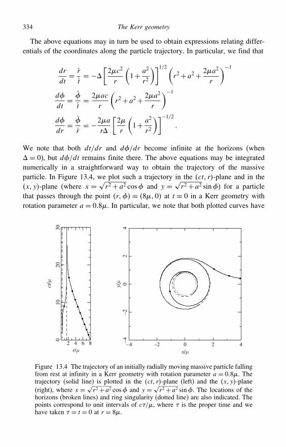
334 The Kerr geometry
The above equations may in turn be used to obtain expressions relating differ-entials of the coordinates along the particle trajectory. In particular, we find that
dr
dt= r
t= −
[2c2
r
(1+ a2
r2
)]1/2(r2+a2+ 2a2
r
)−1d
dt=
t= 2ac
r
(r2+a2+ 2a2
r
)−1d
dr=
r= −2a
r
[2r
(1+ a2
r2
)]−1/2
We note that both dt/dr and d/dr become infinite at the horizons (when = 0), but d/dt remains finite there. The above equations may be integratednumerically in a straightforward way to obtain the trajectory of the massiveparticle. In Figure 13.4, we plot such a trajectory in the ct r-plane and in thex y-plane (where x = √r2+a2 cos and y = √r2+a2 sin) for a particlethat passes through the point r = 80 at t = 0 in a Kerr geometry withrotation parameter a= 08. In particular, we note that both plotted curves have
–4 –2 0 2 4x/µr/µ
y/µ
ct/µ
42
0–2
–4
2 4 6 8
3020
100
Figure 13.4 The trajectory of an initially radially moving massive particle fallingfrom rest at infinity in a Kerr geometry with rotation parameter a= 08. Thetrajectory (solid line) is plotted in the ct r-plane (left) and the x y-plane(right), where x =√r2+a2 cos and y =√r2+a2 sin. The locations of thehorizons (broken lines) and ring singularity (dotted line) are also indicated. Thepoints correspond to unit intervals of c/, where is the proper time and wehave taken = t = 0 at r = 8.
13.13 Equatorial circular motion of massive particles 335
discontinuities at the horizons, which are shown as broken lines. This illustratesthe pathology of the t- and -coordinates in these regions. The points in each plotcorrespond to unit intervals of c/, where is the proper time and we have taken = 0 at r = 8. The proper time increases steadily, without becoming singular;the particle reaches the ring singularity in the equatorial plane at c/= 102. Inthe right-hand plot we also note the effect of frame-dragging on the trajectory ofthe initially radially moving particle.
13.13 Equatorial circular motion of massive particles
For circular motion, we require that r = 0 and, for the particle to remain in acircular orbit, that the radial acceleration r must also vanish. In terms of theeffective potential defined in (13.46), for a circular orbit at r = rc we thus require
Veffrch k= 12c
2k2−1 anddVeff
dr
∣∣∣∣r=rc
= 0 (13.47)
These two equations determine the values of the constants k and h that correspondto a circular orbit at some assigned radius r = rc.Obtaining analytic expressions for k and h is, algebraically, considerably more
complicated than in the Schwarzschild case. The derivation is simplified some-what, however, by working in terms of u = 1/r. Making this substitution into(13.46) and then differentiating the resulting expression with respect to u, wefind that
−c2u+ 12 h
2−a2c2k2−1u2−h−ack2u3 = 12c
2k2−1
−c2+ h2−a2c2k2−1u−3h−ack2u2 = 0
where the second equality holds since dVeff/dr = dVeff/dudu/dr, and there-fore dVeff/du = 0 implies that dVeff/dr = 0. The algebra is further eased byintroducing the variable x = h−ack, so that the two equations above become
−c2u+ 12x
2+2ackx+a2c2u2−x2u3 = 12c
2k2−1 (13.48)
−c2+ x2+2ackx+a2c2u−3x2u2 = 0 (13.49)
Subtracting (13.48) from u times (13.49) and performing a simple rearrangmentof (13.49), we obtain
c2k2 = c21−u+x2u3 (13.50)
2xacku = x2u3u−1− c2a2u− (13.51)
336 The Kerr geometry
These are the basic equations to be used for obtaining analytic expressions forthe constants k and h.
Eliminating k between (13.50) and (13.51), we quickly obtain a quadraticequation for x2,
u2[3u−12−4a2u3
]x4−2c2u
[3u−1a2u−−2ua2u−1
]x2
+ c4a2u−2 = 0
Using the standard formula for the roots of a quadratic equation, one finds (aftersome straightforward but substantial algebra) that
x2 = c2a√u±√2
u1−3u∓2a√u3
(13.52)
As we shall see below, the upper signs corresponds to the counter-rotating circularorbit and the lower signs to the co-rotating one. Furthermore, in order to obtainx we must choose either the positive or negative square root of (13.52). As wemight expect from our discussion of the stability of massive particle orbits in theSchwarzschild case (see Chapter 9), the possibility exists for a circular orbit ata given coordinate radius to be either stable or unstable. It is straightforward toshow that it is the negative root of (13.52) that corresponds to the stable case, inwhich we are most interested. We therefore consider only the solution
x =− ca√u±√
u1−3u∓2a√u31/2
(13.53)
Inserting this solution into (13.50), for a stable circular orbit of inverse coordinateradius u we find that
k= 1−2u∓a√u3
1−3u∓2a√u31/2
(13.54)
the energy of a particle of rest mass m0 being E = km0c2. The corresponding
value of the specific angular momentum for the orbit is obtained by calculatingh= x+ack, which gives
h=∓ c√1+a2u2±2a
√u3√
u1−3u∓2a√u31/2
(13.55)
We note that, as expected, in the limit a→ 0 the expressions (13.54) and (13.55)reduce to the corresponding results in the Schwarzschild case derived in Chapter 9.
13.14 Stability of equatorial massive particle circular orbits 337
13.14 Stability of equatorial massive particle circular orbits
It is worthwhile considering in some detail the stability of equatorial massive-particle orbits. Of particular astrophysical interest is the stability of the circularorbits discussed above and, especially, the coordinate radius of the innermoststable circular orbit in the co- and counter-rotating cases.
For a circular orbit of coordinate radius r = rc we require the condition (13.47).In addition, for marginal stability we require that (for r = rc)
d2Veff
dr2= d2Veff
du2
(du
dr
)2
+ dVeff
du
d2u
dr2= u3
(d2Veff
du2+2
dVeff
du
)= 0
where u= 1/r . Since dVeff/du= 0 for a circular orbit, this additional requirementamounts to d2Veff/du
2 = 0. From (13.49), this reads
x2+2ackx+a2c2−6x2u= 0
which may be more conveniently written as
u= x2+2ackx+a2c2
6x2= h2−a2c2k2−1
6x2
Inserting the expressions (13.53–13.55) for x, k and h respectively into thisequation and simplifying, one finds that
1−3a2u2−6u∓8a√u3 = 0
Finally, using u= 1/r, one obtains an implicit equation for the coordinate radiusr of the innermost stable circular orbit,
r2−6r−3a2∓8a√r = 0 (13.56)
where, once again, the upper sign corresponds to the counter-rotating orbit andthe lower sign to the co-rotating orbit. In the limit a= 0, we see that we recoverr = 6 for the innermost stable circular orbit in the Schwarzschild case. In theextreme Kerr limit a = we find, by inspection, that r = 9 for the counter-rotating orbit and r = for the co-rotating case.
The general solution to the above quartic equation in√r can be found analyti-
cally by standard methods, but the resulting expressions are algebraically messy.It is more instructive instead to solve the equation numerically and plot the resultsfor a range of a/ values, as shown in Figure 13.5 (left-hand panel). Also ofparticular interest is the energy E of a particle in the innermost co- and counter-rotating stable circular orbits. Using the expression (13.54), in the right-handpanel of Figure 13.5 we plot k= E/m0c
2 for these orbits as a function of a/.The difference between the energy E = km0c
2 of a particle in an orbit and theenergy m0c
2 of the particle at rest at infinity is the gravitational binding energy
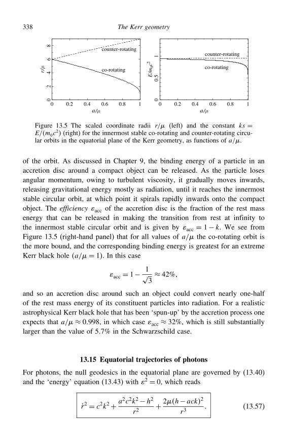
338 The Kerr geometry
counter-rotating
co-rotating
counter-rotating
co-rotating
0a /µ
00.
51
0.2 0.4 0.6 0.8 10
02
46
8
a /µ
r /µ
E /m
0c2
0.2 0.4 0.6 0.8 1
Figure 13.5 The scaled coordinate radii r/ (left) and the constant ks =E/m0c
2 (right) for the innermost stable co-rotating and counter-rotating circu-lar orbits in the equatorial plane of the Kerr geometry, as functions of a/.
of the orbit. As discussed in Chapter 9, the binding energy of a particle in anaccretion disc around a compact object can be released. As the particle losesangular momentum, owing to turbulent viscosity, it gradually moves inwards,releasing gravitational energy mostly as radiation, until it reaches the innermoststable circular orbit, at which point it spirals rapidly inwards onto the compactobject. The efficiency )acc of the accretion disc is the fraction of the rest massenergy that can be released in making the transition from rest at infinity tothe innermost stable circular orbit and is given by )acc = 1− k. We see fromFigure 13.5 (right-hand panel) that for all values of a/ the co-rotating orbit isthe more bound, and the corresponding binding energy is greatest for an extremeKerr black hole a/= 1. In this case
)acc = 1− 1√3≈ 42%
and so an accretion disc around such an object could convert nearly one-halfof the rest mass energy of its constituent particles into radiation. For a realisticastrophysical Kerr black hole that has been ‘spun-up’ by the accretion process oneexpects that a/ ≈ 0998, in which case )acc ≈ 32%, which is still substantiallylarger than the value of 57% in the Schwarzschild case.
13.15 Equatorial trajectories of photons
For photons, the null geodesics in the equatorial plane are governed by (13.40)and the ‘energy’ equation (13.43) with )2 = 0, which reads
r2 = c2k2+ a2c2k2−h2
r2+ 2h−ack2
r3 (13.57)
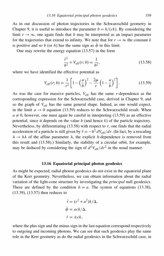
13.16 Equatorial principal photon geodesics 339
As in our discussion of photon trajectories in the Schwarzschild geometry inChapter 9, it is useful to introduce the parameter b = h/ck. By considering thelimit r →, one again finds that b may be interpreted as an impact parameterfor the trajectories that extend to infinity. We note that for r→ the constant kis positive and so b (or h) has the same sign as in this limit.
One may rewrite the energy equation (13.57) in the form
r2
h2+Veffr b=
1b2
(13.58)
where we have identified the effective potential as
Veffr b=1r2
[1−
(ab
)2− 2r
(1− a
b
)2] (13.59)
As was the case for massive particles, Veff has the same r-dependence as thecorresponding expression for the Schwarzschild case, derived in Chapter 9, andso the graph of Veff has the same general shape. Indeed, as one would expect,in the limit a→ 0 equation (13.59) reduces to the Schwarzschild result. Whena = 0, however, one must again be careful in interpreting (13.59) as an effectivepotential, since it depends on the value b (and hence k) of the particle trajectory.Nevertheless, by differentiating (13.58) with respect to , one finds that the radialacceleration of a particle is still given by r =−h2 dVeff/dr. (In fact, by a rescaling→ h of the affine parameter , the explicit h-dependence is removed fromthis result and (13.58).) Similarly, the stability of a circular orbit, for example,may be deduced by considering the sign of d2Veff/dr
2 in the usual manner.
13.16 Equatorial principal photon geodesics
As might be expected, radial photon geodesics do not exist in the equatorial planeof the Kerr geometry. Nevertheless, we can obtain information about the radialvariation of the light-cone structure by investigating the principal null geodesics.These are defined by the condition b = a. The system of equations (13.38),(13.39), (13.57) then reduces to
t = r2+a2k/
= ack/
r = ±ckwhere the plus sign and the minus sign in the last equation correspond respectivelyto outgoing and incoming photons. We can see that such geodesics play the samerole in the Kerr geometry as do the radial geodesics in the Schwarzschild case, in
340 The Kerr geometry
that the radial coordinate is described at a uniform rate with respect to the affineparameter.
Choosing r =+ck for outgoing photons, we find that
dt
dr= t
r= r2+a2
c
d
dr=
r= a
Using the fact that > 0 in region I, it follows that dr/dt > 0 in region I, thusconfirming that these equations correspond to outgoing photons. If we restrict ourattention to the case a2 <2, the equations can be immediately integrated to give
ct = r+(+ 2√
2−a2
)ln
∣∣∣∣ rr+ −1
∣∣∣∣+(− 2√
2−a2
)ln
∣∣∣∣ rr− −1
∣∣∣∣+ constant (13.60)
= a
2√2−a2
ln
∣∣∣∣r− r+r− r−
∣∣∣∣+ constant (13.61)
The solution corresponding to incoming photons is obtained by choosing r =−ckand has the same form as above but with t→−t and →−. In Figure 13.6 weplot an incoming principal null geodesic in the ct r-plane and in the x y-plane(with x=√r2+a2 cos and y=√r2+a2 sin) for a photon that passes through
y/µ
ct/µ
r/µ x/µ– 4
–4–2
02
4
–2 0 2 42
010
2030
4 6 8
Figure 13.6 A principal null geodesic in a Kerr geometry with rotation param-eter a = 08. The trajectory (solid line) is plotted in the ct r-plane (left)and in the x y-plane (right); x =√r2+a2 cos and y =√r2+a2 sin. Thelocations of the horizons (broken lines) and the ring singularity (dotted line) arealso indicated.
13.17 Equatorial circular motion of photons 341
the point r = 80 at t = 0 in a Kerr geometry with rotation parametera= 08.
We note that, in the limit a→ 0, (13.60) reduces to the equation for a radialphoton trajectory in the Schwarzschild geometry, as presented in Section 11.3.Indeed, the null geodesics considered above play the same role as the null radialgeodesics in the Schwarzschild case, giving information about the radial variationof the light-cone structure. We can draw a spacetime diagram of the light-conestructure using these equations and we find in region I a diagram analogous to thatobtained for the Schwarzschild geometry in t r coordinates in Chapter 11:the light-cones narrow down as r→ r+. On r = r+ both t and become infinite,again indicating that this is a coordinate singularity.
13.17 Equatorial circular motion of photons
For circular photon motion we require r = 0 and, for the photon to remain in acircular orbit, the radial acceleration r must also vanish. In terms of the effectivepotential defined in (13.59), for a circular orbit at r = rc we thus require
Veffrc b=1b2
anddVeff
dr
∣∣∣∣r=rc
= 0 (13.62)
These two equations determine a single value r = rc (different for prograde andretrograde orbits) for which there exists a circular orbit, and the correspondingvalue of the constant b.
Using the expression (13.59), the above conditions yield respectively
rc = 3b−a
b+a (13.63)
b+a3 = 272b−a (13.64)
These equations may be solved by setting y = b+ a in (13.64), solving theresulting cubic equation and substituting the resulting value of b into (13.63). Onemay easily verify that the result can be written as
rc = 21+ cos
[23cos−1
(± a
)] (13.65)
b = 3√rc−a (13.66)
where the upper sign in (13.65) corresponds to retrograde orbits and the lowersign to prograde orbits. In the limit a→ 0 we recover the conditions for a circularphoton orbit in the Schwarzschild case, obtained in Chapter 9, namely rc = 3and b = 3
√3. As in the Schwarzschild case, circular photon orbits in the Kerr
geometry are unstable.
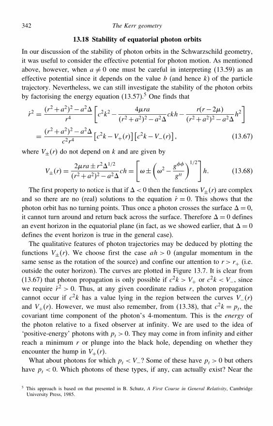
342 The Kerr geometry
13.18 Stability of equatorial photon orbits
In our discussion of the stability of photon orbits in the Schwarzschild geometry,it was useful to consider the effective potential for photon motion. As mentionedabove, however, when a = 0 one must be careful in interpreting (13.59) as aneffective potential since it depends on the value b (and hence k) of the particletrajectory. Nevertheless, we can still investigate the stability of the photon orbitsby factorising the energy equation (13.57).5 One finds that
r2 = r2+a22−a2
r4
[c2k2− 4ra
r2+a22−a2ckh− rr−2
r2+a22−a2h2]
= r2+a22−a2
c2r4[c2k−V+r
] [c2k−V−r
] (13.67)
where V±r do not depend on k and are given by
V±r=2ra± r21/2
r2+a22−a2ch=
[±
(2− g
gtt
)1/2]h (13.68)
The first property to notice is that if < 0 then the functions V±r are complexand so there are no (real) solutions to the equation r = 0. This shows that thephoton orbit has no turning points. Thus once a photon crosses the surface = 0,it cannot turn around and return back across the surface. Therefore = 0 definesan event horizon in the equatorial plane (in fact, as we showed earlier, that = 0defines the event horizon is true in the general case).
The qualitative features of photon trajectories may be deduced by plotting thefunctions V±r. We choose first the case ah > 0 (angular momentum in thesame sense as the rotation of the source) and confine our attention to r > r+ (i.e.outside the outer horizon). The curves are plotted in Figure 13.7. It is clear from(13.67) that photon propagation is only possible if c2k > V+ or c2k < V−, sincewe require r2 > 0. Thus, at any given coordinate radius r, photon propagationcannot occur if c2k has a value lying in the region between the curves V−rand V+r. However, we must also remember, from (13.38), that c2k = pt, thecovariant time component of the photon’s 4-momentum. This is the energy ofthe photon relative to a fixed observer at infinity. We are used to the idea of‘positive-energy’ photons with pt > 0. They may come in from infinity and eitherreach a minimum r or plunge into the black hole, depending on whether theyencounter the hump in V+r.
What about photons for which pt < V−? Some of these have pt > 0 but othershave pt < 0. Which photons of these types, if any, can actually exist? Near the
5 This approach is based on that presented in B. Schutz, A First Course in General Relativity, CambridgeUniversity Press, 1985.
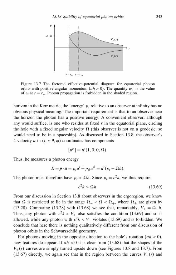
13.18 Stability of equatorial photon orbits 343
r
ω + h
V
V+(r)
V–(r)
r = r+ r = rs+
Figure 13.7 The factored effective-potential diagram for equatorial photonorbits with positive angular momentum ah > 0. The quantity + is the valueof at r = r+. Photon propagation is forbidden in the shaded region.
horizon in the Kerr metric, the ‘energy’ pt relative to an observer at infinity has noobvious physical meaning. The important requirement is that to an observer nearthe horizon the photon has a positive energy. A convenient observer, althoughany would suffice, is one who resides at fixed r in the equatorial plane, circlingthe hole with a fixed angular velocity (this observer is not on a geodesic, sowould need to be in a spaceship). As discussed in Section 13.8, the observer’s4-velocity u in t r coordinates has components
u= ut100
Thus, he measures a photon energy
E = p ·u= ptut+pu
= utpt−h
The photon must therefore have pt > h. Since pt = c2k, we thus require
c2k > h (13.69)
From our discussion in Section 13.8 about observers in the ergoregion, we knowthat is restricted to lie in the range − < < +, where ± are given by(13.28). Comparing (13.28) with (13.68) we see that, remarkably, V± = ±h.Thus, any photon with c2k > V+ also satisfies the condition (13.69) and so isallowed, while any photon with c2k < V− violates (13.69) and is forbidden. Weconclude that here there is nothing qualitatively different from our discussion ofphoton orbits in the Schwarzschild geometry.
For photons moving in the opposite direction to the hole’s rotation ah < 0,new features do appear. If ah < 0 it is clear from (13.68) that the shapes of theV±r curves are simply turned upside down (see Figures 13.8 and 13.7). From(13.67) directly, we again see that in the region between the curves V−r and
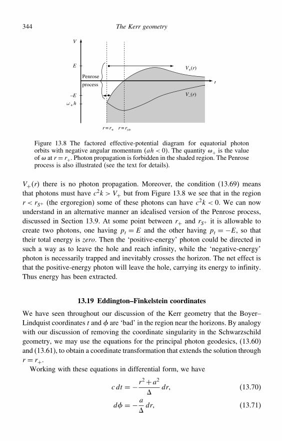
344 The Kerr geometry
V
E
–E
Penrose
process r
ω + h
V+(r)
V–(r)
r = r+ r = rs+
Figure 13.8 The factored effective-potential diagram for equatorial photonorbits with negative angular momentum ah < 0. The quantity + is the valueof at r = r+. Photon propagation is forbidden in the shaded region. The Penroseprocess is also illustrated (see the text for details).
V+r there is no photon propagation. Moreover, the condition (13.69) meansthat photons must have c2k > V+ but from Figure 13.8 we see that in the regionr < rS+ (the ergoregion) some of these photons can have c2k < 0. We can nowunderstand in an alternative manner an idealised version of the Penrose process,discussed in Section 13.9. At some point between r+ and rS+ it is allowable tocreate two photons, one having pt = E and the other having pt = −E, so thattheir total energy is zero. Then the ‘positive-energy’ photon could be directed insuch a way as to leave the hole and reach infinity, while the ‘negative-energy’photon is necessarily trapped and inevitably crosses the horizon. The net effect isthat the positive-energy photon will leave the hole, carrying its energy to infinity.Thus energy has been extracted.
13.19 Eddington–Finkelstein coordinates
We have seen throughout our discussion of the Kerr geometry that the Boyer–Lindquist coordinates t and are ‘bad’ in the region near the horizons. By analogywith our discussion of removing the coordinate singularity in the Schwarzschildgeometry, we may use the equations for the principal photon geodesics, (13.60)and (13.61), to obtain a coordinate transformation that extends the solution throughr = r+.Working with these equations in differential form, we have
c dt = −r2+a2
dr (13.70)
d = − a
dr (13.71)
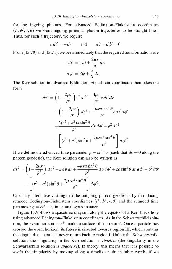
13.19 Eddington–Finkelstein coordinates 345
for the ingoing photons. For advanced Eddington–Finkelstein coordinatest′′ r we want ingoing principal photon trajectories to be straight lines.Thus, for such a trajectory, we require
c dt′ = −dr and d = d′ = 0
From (13.70) and (13.71), we see immediately that the required transformations are
c dt′ = c dt+ 2r
dr
d′ = d+ a
dr
The Kerr solution in advanced Eddington–Finkelstein coordinates then takes theform
ds2 =(1− 2r
2
)c2 dt′2− 4r
2c dt′ dr
−(1+ 2r
2
)dr2+ 4ra sin2
2c dt′ d′
+2r2+a2a sin2 2
dr d′ −2 d2
−[r2+a2 sin2 + 2ra2 sin4
2
]d′2
If we define the advanced time parameter p= ct′ + r (such that dp= 0 along thephoton geodesic), the Kerr solution can also be written as
ds2 =(1− 2r
2
)dp2−2dpdr+ 4ra sin2
2dpd′ +2a sin2 dr d′ −2 d2
−[r2+a2 sin2 + 2ra2 sin4
2
]d′2
One may alternatively straighten the outgoing photon geodesics by introducingretarded Eddington–Finkelstein coordinates t∗∗ r and the retarded timeparameter q = ct∗ − r, in an analogous manner.
Figure 13.9 shows a spacetime diagram along the equator of a Kerr black holeusing advanced Eddington–Finkelstein coordinates. As in the Schwarzschild solu-tion, the event horizon at r+ marks a surface of ‘no return’. Once a particle hascrossed the event horizon, its future is directed towards region III, which containsthe singularity – you can never return back to region I. Unlike the Schwarzschildsolution, the singularity in the Kerr solution is timelike (the singularity in theSchwarzschild solution is spacelike). In theory, this means that it is possible toavoid the singularity by moving along a timelike path; in other words, if we
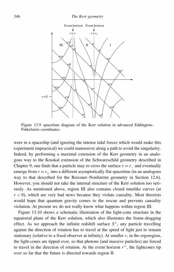
346 The Kerr geometry
II I
r = r–
III
r = r+
Event horizon Event horizon
r = 0
Figure 13.9 spacetime diagram of the Kerr solution in advanced Eddington–Finkelstein coordinates.
were in a spaceship (and ignoring the intense tidal forces which would make thisexperiment impractical) we could manoeuvre along a path to avoid the singularity.Indeed, by performing a maximal extension of the Kerr geometry in an analo-gous way to the Kruskal extension of the Schwarzschild geometry described inChapter 9, one finds that a particle may re-cross the surface r = r− and eventuallyemerge from r = r+ into a different asymptotically flat spacetime (in an analogousway to that described for the Reissner–Nordström geometry in Section 12.6).However, you should not take the internal structure of the Kerr solution too seri-ously. As mentioned above, region III also contains closed timelike curves (atr < 0), which are very bad news because they violate causality. Most theoristswould hope that quantum gravity comes to the rescue and prevents causalityviolation. At present we do not really know what happens within region III.
Figure 13.10 shows a schematic illustration of the light-cone structure in theequatorial plane of the Kerr solution, which also illustrates the frame-draggingeffect. As we approach the infinite redshift surface S+, any particle travellingagainst the direction of rotation has to travel at the speed of light just to remainstationary (relative to a fixed observer at infinity). At smaller r, in the ergoregion,the light-cones are tipped over, so that photons (and massive particles) are forcedto travel in the direction of rotation. At the event horizon r+, the lightcones tipover so far that the future is directed towards region II.
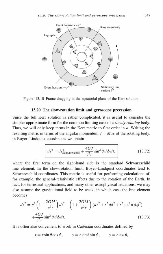
13.20 The slow-rotation limit and gyroscope precession 347
Ring singularityEvent horizon r = r –
Stationary limitsurface S+
Ergosphere
Event horizon r = r+
Figure 13.10 Frame dragging in the equatorial plane of the Kerr solution.
13.20 The slow-rotation limit and gyroscope precession
Since the full Kerr solution is rather complicated, it is useful to consider thesimpler approximate form for the common limiting case of a slowly rotating body.Thus, we will only keep terms in the Kerr metric to first order in a. Writing theresulting metric in terms of the angular momentum J =Mac of the rotating body,in Boyer–Lindquist coordinates we obtain
ds2 = ds2Schwarzschild+4GJ
c2rsin2 ddt (13.72)
where the first term on the right-hand side is the standard Schwarzschildline element. In the slow-rotation limit, Boyer–Lindquist coordinates tend toSchwarzschild coordinates. This metric is useful for performing calculations of,for example, the general-relativistic effects due to the rotation of the Earth. Infact, for terrestrial applications, and many other astrophysical situations, we mayalso assume the gravitational field to be weak, in which case the line elementbecomes
ds2 = c2(1− 2GM
c2r
)dt2−
(1+ 2GM
c2r
)dr2+ r2 d2+ r2 sin2 d2
+4GJ
c2rsin2 ddt (13.73)
It is often also convenient to work in Cartesian coordinates defined by
x = r sin cos y = r sin sin y = r cos
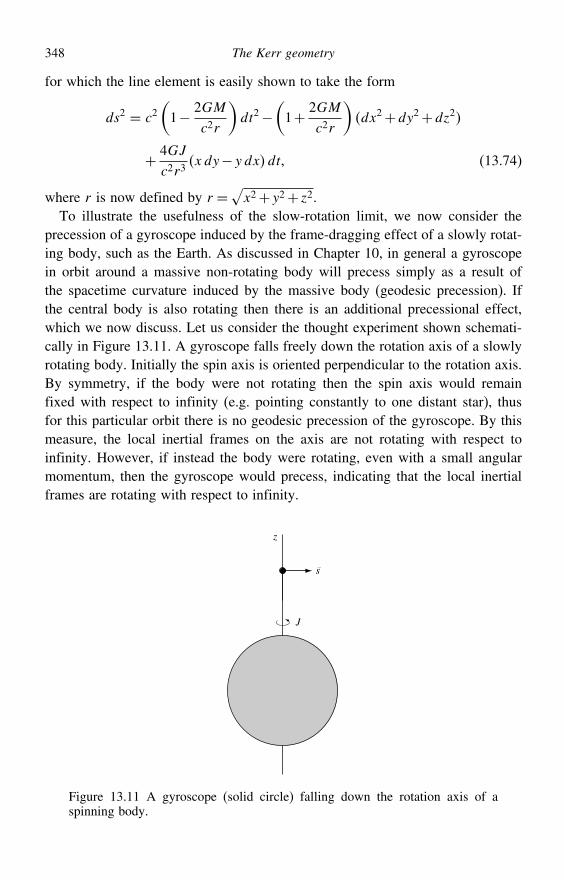
348 The Kerr geometry
for which the line element is easily shown to take the form
ds2 = c2(1− 2GM
c2r
)dt2−
(1+ 2GM
c2r
)dx2+dy2+dz2
+ 4GJ
c2r3xdy−y dxdt (13.74)
where r is now defined by r =√x2+y2+ z2.To illustrate the usefulness of the slow-rotation limit, we now consider the
precession of a gyroscope induced by the frame-dragging effect of a slowly rotat-ing body, such as the Earth. As discussed in Chapter 10, in general a gyroscopein orbit around a massive non-rotating body will precess simply as a result ofthe spacetime curvature induced by the massive body (geodesic precession). Ifthe central body is also rotating then there is an additional precessional effect,which we now discuss. Let us consider the thought experiment shown schemati-cally in Figure 13.11. A gyroscope falls freely down the rotation axis of a slowlyrotating body. Initially the spin axis is oriented perpendicular to the rotation axis.By symmetry, if the body were not rotating then the spin axis would remainfixed with respect to infinity (e.g. pointing constantly to one distant star), thusfor this particular orbit there is no geodesic precession of the gyroscope. By thismeasure, the local inertial frames on the axis are not rotating with respect toinfinity. However, if instead the body were rotating, even with a small angularmomentum, then the gyroscope would precess, indicating that the local inertialframes are rotating with respect to infinity.
z
s
J
Figure 13.11 A gyroscope (solid circle) falling down the rotation axis of aspinning body.
13.20 The slow-rotation limit and gyroscope precession 349
We can use the metric (13.74) to calculate the precession rate of the gyro-scope on its downward ‘polar plunge’ trajectory. As shown in Section 10.5, thespin 4-vector s is parallel-transported along the geodesic trajectory. Thus, itscomponents satisfy
ds
d+
#su# = 0 (13.75)
For the physical arrangement under consideration, the initial 4-velocity u and thespin 4-vector s of the gyroscope in Cartesian coordinates have the forms
u= ut00 uz and s= 0 sx sy0
Moreover, these forms remain valid at all later times, since the trajectory is apolar plunge and s ·u is conserved along it. Thus, in (13.75), the only equationswe need to consider are
dsx
d+ x
xtsxut+ x
xzsxuz+ x
ytsyut+ x
yzsyuz = 0 (13.76)
dsy
d+ y
xtsxut+ y
xzsxuz+ y
ytsyut+ y
yzsyuz = 0 (13.77)
To continue with our calculation, we must first find the connection coeffi-cients appearing in the above equations. This is most easily achieved using the‘Lagrangian’ approach, writing down the Euler–Lagrange equation for x andremembering that on the polar axis all terms proportional to some positive powerof x or y are zero and r = z. One finds that the only non-zero connection coeffi-cients of the form x
are( x
yt
)z-axis =
2GJ
c2z3and
( x
xz
)z-axis =−
2GM
c2zz+2GM/c2
By considering the symmetry properties of the metric (13.74), one immediatelydeduces that, on the polar axis, the only non-zero connection coefficients of theform y
are
yxtz-axis =−
2GJ
c2z3and
( y
yz
)z-axis =−
2GM
c2zz+2GM/c2
These connection coefficients can now be substituted into equations (13.76,13.77), which can be solved once ut and uz have been determined from thegeodesic equations. Assuming, however, that the speed of the falling gyroscopeis non-relativistic, then to leading order in 1/c we may take ut ≈ 1 and uz ≈ 0.Thus, in this approximation, equations (13.76, 13.77) reduce to
dsx
d=−2GJ
c2z3sy and
dsy
d= 2GJ
c2z3sx
350 The Kerr geometry
Hence, as it falls, the gyroscope precesses in the same direction as the body isrotating, i.e. the local inertial frames are dragged with respect to infinity. This iscalled the Lens–Thirring effect. At a height z the rate of precession is
LT =2GJ
c2z3
It should be noted that we have calculated this precession rate in a Cartesiancoordinate system in which the centre of the gravitating body is at rest andthe gyroscope is falling. Fortunately, an observer free-falling with the gyroscopewould measure the same precession rate since the Lorentz transformation thatconnects the two frames is a boost along the z-axis, which does not affect thetransverse components sx and sy of the spin vector. Of course, the Lens–Thirringeffect also results in the precession of gyroscopes following trajectories otherthan the polar plunge considered here, but determining the rate of precession ingeneral requires a considerably longer calculation (see Exercise 17.26).
Exercises
13.1 Verify that the Boyer–Lindquist form of the Kerr metric satisfies the empty-spaceEinstein field equations.Note: This exercise is only for the truly dedicated reader!
13.2 Show that the Boyer–Lindquist form of the Kerr metric can be written in the forms(13.12) and (13.13).
13.3 Calculate the contravariant components g of the Kerr metric in Boyer–Lindquistcoordinates.
13.4 Show that, in the limit → 0, the Kerr metric tends to the Minkowksi metric.13.5 Show that the Kerr–Schild form of the Kerr metric can be transformed into the
Boyer–Lindquist form by the coordinate transformations (13.16 –13.19).13.6 Consider the 2-surfaces defined by t = constant and r = r± in the Kerr geometry.
Show that, for each surface, the circumference around the ‘poles’ is less than thecircumference around the equator. Show that the same is true for the 2-surfacesdefined by t = constant and r = rS±.
13.7 Show that the proper area of the event horizon r = r+ in the Kerr geometry isgiven by
A= 4(r2++a2
)
Hence show that, for fixed , the area A is a maximum for a= 0. Conversely, forfixed A, show that is a minimum for a= 0. Comment on your results.
Exercises 351
13.8 An observer is at fixed (r, ) coordinates in the ergoregion of a Kerr black holeand has angular velocity = d/dt with respect to a second observer at rest atinfinity. Show that the allowed range for is given by − <<+, where
± = ± c
(
(2
)1/2
and , and (2 have their usual meanings in the Kerr metric.13.9 Use your answer to Exercise 13.7 to show that the area of the event horizon r = r+
in the Kerr geometry may be written as
A= 8Gc4
⎡⎣M2+√M4−
(cJ
G
)2⎤⎦
where M and J are the mass and angular momentum of the black hole. Henceshow that if the mass and angular momentum change by M and J respectivelythen the corresponding change in the proper area of the horizon is given by
A= 8Gc
a
H
√2−a2
(M−H
J
c2
)
where H is the ‘angular velocity of the horizon’, defined in (13.29). Thus showthat the area of the event horizon must increase in the Penrose process.
13.10 Show that, in the equatorial plane =/2 of the Kerr geometry, the contravariantmetric components in Boyer–Lindquist coordinates are
gtt = 1c2
(r2+a2+ 2a2
r
) gt = 2a
cr
grr = −
r2 g =− 1
(1− 2
r
)
13.11 Show that the geodesic equations for particle motion in the equatorial plane of theKerr geometry may be written in Boyer–Lindquist coordinates as
t = 1
[(r2+a2+ 2a2
r
)k− 2a
crh
]
= 1
[2acr
k+(1− 2
r
)h
]
r2 = c2k2− 2+ 22r
+ a2c2k2− 2−h2
r2+ 2h−ack2
r3
where 2 = c2 for a massive particle and = 0 for a photon. Verify that theseequations reduce to the Schwarzschild case in the limit a→ 0.
13.12 The trajectory of an infalling particle of mass m in the equatorial plane of aKerr black hole is characterised by the usual parameters k and h. If the particle
352 The Kerr geometry
eventually falls into the black hole, show that the mass and the angular momentumof the hole are changed in such a way that
M→M+kmc2 J → J +mh
Show further that the corresponding change a in the rotation parameter of theblack hole is given by
a= m
cMh−ack
If the particle falls into an extreme Kerr black hole, for which a= , show that anaked singularity would be created if
h > 2ck
However, by determining the maximum value of the effective potential Veffrh k
defined in (13.46) for a = , show that a particle with h > 2ck can never fallinto the black hole.
13.13 For a Kerr black hole, using the Boyer–Lindquist coordinates show that, for aparticle in circular orbit in the = /2 plane, the coordinate angular velocity= d/dt satisfies
= c1/2
a1/2± r3/2
This is the Kerr-metric analogue to 2 = GM/r3 for the Schwarzschild metric.Here the plus sign corresponds to prograde orbits, the minus to retrograde orbits.
13.14 If a particle’s motion is initially in the = /2 plane in a Kerr metric, show thatthe motion will remain in this plane.
13.15 Show that the values of the parameters k and h for a circular orbit of coordinateradius r = rc, given in (13.54) and (13.55) respectively, satisfy the requirements
Veffrch k= 12c
2k2−1 anddVeff
dr
∣∣∣∣r=rc
= 0
Show further that for the orbit to be stable one requires
r2c −6rc−3a2∓8a√rc = 0
13.16 An observer (not necessarily free-falling) orbits a Kerr black hole in the equatorialplane in a circular orbit. His ‘angular velocity with respect to a distant observer’is = d/dt. Find the components ut uut and u in terms of r and a.
13.17 Suppose that the circular orbit considered in Exercise 13.16 lies outside the horizonr+ but inside the stationary limit rS+ . Show that under these circumstances mustbe non-zero, i.e. the observer cannot remain at rest relative to a distant observer.If the orbiting observer is in the region r− < r < r+, show that the orbit cannot becircular.
Exercises 353
13.18 Show that the effective potential for photon orbits in the equatorial plane of theKerr geometry is given by
Veffr b=1r2
[1−
(ab
)2− 2r
(1− a
b
)2]
13.19 For a circular photon orbit of coordinate radius r = rc in the Kerr geometry,show that
rc = 21+ cos
[23cos−1
(± a
)]
b = 3√rc−a
where the upper sign in the first equation corresponds to retrograde orbits and thelower sign to prograde orbits. Hence show that, for an extreme Kerr black hole(a= ), rc = 4 for a retrograde orbit and rc = for a prograde orbit.
13.20 For a photon orbit in the equatorial plane of the Kerr geometry, show that
r2 = r2+a22−a2
c2r4 c2k−V+r c
2k−V−r
where
V±r=2ra± r21/2
r2+a22−a2ch=
[±
(2− g
gtt
)1/2]h
13.21 The general axisymmetric stationary metric can be written in the form
ds2 = Adt2−Bd−dt2−C dr2−Dd2
where A, B, C, D and are functions only of the coordinates r and . Aliceis an astronaut in a powered spaceship that maintains fixed r coordinates inthe equatorial plane = /2 (at a position for which gtt > 0). She simultaneouslyemits two photons in opposite tangential directions in the equatorial plane and usesa prearranged system of mirrors to cause each photon to move along a circular(non-geodesic) path of constant r. Show that the coordinate angular velocities ofthe two photons are given by
d
dt= ±
(A
B
)1/2
Hence show that the two photons do not arrive back with Alice simultaneouslybut are separated by a time interval
= 4BcA−B21/2
as measured by Alice’s on-board clock. Comment on the physical significance ofthis result.
354 The Kerr geometry
13.22 Bob is in a powered spaceship following a circular orbit r = constant in theequatorial plane of the geometry in Exercise 13.21. His angular velocity is suchthat the component u of his 4-velocity is zero. Using the same arrangement ofmirrors as in Exercise 13.21, he performs an experiment similar to Alice’s. Showthat for Bob the two photons arrive back to him simultaneously.
13.23 Which, if any, of the photons considered in Exercises 13.21 and 13.22 is redshiftedfrom its original frequency on arriving back with Alice or Bob? Explain yourreasoning.
13.24 An isolated thin rigid spherical shell has mass M and radius R. If the shell is setspinning slowly, with angular momentum J , show that inertial frames within theshell rotate with angular velocity
= 2GJ
c2R3
Comment briefly on how this result is related to Mach’s principle.
14
The Friedmann–Robertson–Walker geometry
We now discuss the application of general relativity to modelling the behaviourof the universe as a whole. In order to do this, we make some far-reachingassumptions, but only those consistent with our observations of the universe. Asin our derivations of the Schwarzschild and Kerr geometries, we begin by usingsymmetry arguments to restrict the possible forms for the metric describing theoverall spacetime geometry of the universe.1
14.1 The cosmological principle
When we look up at the sky we see that the stars around us are grouped into alarge-density concentration – the Milky Way Galaxy. On a slightly larger scale,we see that our Galaxy belongs to a small group of galaxies (called the LocalGroup). Our Galaxy and our nearest large neighbour, the Andromeda galaxy,dominate the mass of the Local Group. On still larger scales we see that ourLocal Group sits on the outskirts of a giant supercluster of galaxies centred in theconstellation of Virgo. Evidently, on small scales matter is distributed in a highlyirregular way but, as we look on larger and larger scales, the matter distributionlooks more and more uniform. In fact, we have very good evidence (particularlyfrom the constancy of the temperature of the cosmic microwave background indifferent directions on the sky) that the universe is isotropic on the very largestscales, to high accuracy. If the universe has no preferred centre then isotropy alsoimplies homogeneity. We therefore have good physical reasons to study simplecosmological models in which the universe is assumed to be homogeneous and
1 For a detailed discussion, see, for example, J. N. Islam, An Introduction to Mathematical Cosmology,Cambridge University Press, 1992.
355
356 The Friedmann–Robertson–Walker geometry
isotropic2. We thus assume the cosmological principle, which states that at anyparticular time the universe looks the same from all positions in space at aparticular time and all directions in space at any point are equivalent.
14.2 Slicing and threading spacetime
The intuitive statement of the cosmological principle given above needs to bemade more precise. In particular, how does one define a ‘particular time’ in generalrelativity that is valid globally, when there are no global inertial frames? Also,since observers moving relative to one another will view the universe differently,according to which observers do we demand the universe to appear isotropic?
In general relativity the concept of a ‘moment of time’ is ambiguous and isreplaced by the notion of a three-dimensional spacelike hypersurface. To definea ‘time’ parameter that is valid globally, we ‘slice up’ spacetime by introducinga series of non-intersecting spacelike hypersurfaces that are labelled by someparameter t. This parameter then defines a universal time in that ‘a particulartime’ means a given spacelike hypersurface. It should be noted, however, thatwe may construct the hypersurfaces t = constant in any number of ways. In ageneral spacetime there is no preferred ‘slicing’ and hence no preferred ‘time’coordinate t.
It is useful at this point to introduce the idealised concept of fundamentalobservers, who are assumed to have no motion relative to the overall cosmologicalfluid associated with the ‘smeared-out’ motion of all the galaxies and other matterin the universe. A fundamental observer would, for example, measure no dipolemoment in his observations of the cosmic microwave background radiation; anobserver with a non-zero peculiar velocity would observe such a dipole as aresult of the Doppler effect arising from his motion relative to the cosmologicalfluid. Adopting Weyl’s postulate, the timelike worldlines of these observers areassumed to form a bundle, or congruence, in spacetime that diverges from a pointin the (finite or infinitely distant) past or converges to such a point in the future.These worldlines are non-intersecting, except possibly at a singular point in thepast or future or both. Thus, there is a unique worldline passing through each(non-singular) spacetime point. The set of worldlines is sometimes described asproviding threading for the spacetime.
The hypersurfaces t= constant may now be naturally constructed in such a waythat the 4-velocity of any fundamental observer is orthogonal to the hypersurface.
2 It is worth noting that isotropy about every point automatically implies homogeneity. However, homogeneitydoes not necessarily imply isotropy. For example, a universe with a large-scale magnetic field that pointedin one direction everywhere and had the same magnitude at every point would be homogeneous but notisotropic.
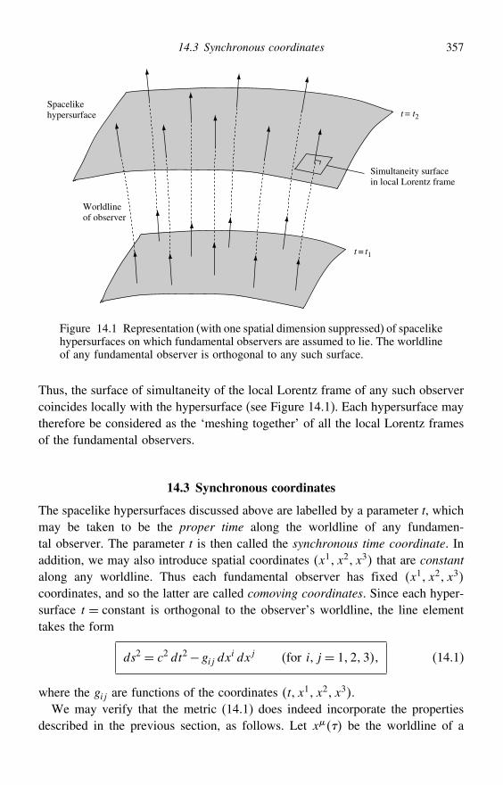
14.3 Synchronous coordinates 357
Simultaneity surfacein local Lorentz frame
t = t2
t = t1
Spacelikehypersurface
Worldlineof observer
Figure 14.1 Representation (with one spatial dimension suppressed) of spacelikehypersurfaces on which fundamental observers are assumed to lie. The worldlineof any fundamental observer is orthogonal to any such surface.
Thus, the surface of simultaneity of the local Lorentz frame of any such observercoincides locally with the hypersurface (see Figure 14.1). Each hypersurface maytherefore be considered as the ‘meshing together’ of all the local Lorentz framesof the fundamental observers.
14.3 Synchronous coordinates
The spacelike hypersurfaces discussed above are labelled by a parameter t, whichmay be taken to be the proper time along the worldline of any fundamen-tal observer. The parameter t is then called the synchronous time coordinate. Inaddition, we may also introduce spatial coordinates x1 x2 x3 that are constantalong any worldline. Thus each fundamental observer has fixed x1 x2 x3
coordinates, and so the latter are called comoving coordinates. Since each hyper-surface t = constant is orthogonal to the observer’s worldline, the line elementtakes the form
ds2 = c2 dt2−gij dxi dxj for i j = 123 (14.1)
where the gij are functions of the coordinates t x1 x2 x3.We may verify that the metric (14.1) does indeed incorporate the properties
described in the previous section, as follows. Let x be the worldline of a
358 The Friedmann–Robertson–Walker geometry
fundamental observer, where is the proper time along the worldline. Then, byconstruction, x is given by
x0 = x1 = constant x2 = constant x3 = constant (14.2)
Since dxi = 0 along the worldline, we obtain ds = c d = c dt and so t = ,thereby showing that the proper time along the worldline is indeed equal to t.Thus, from (14.2), it is clear that the 4-velocity of a fundamental observer incomoving coordinates is
u≡[dx
d
]= 1000 (14.3)
Since any vector lying in the hypersurface t = constant has the form a =0 a1 a2 a3, we see that
gua = 0
because g0i = 0 for i = 123. Hence, the observer’s 4-velocity is orthogonal tothe hypersurface, as we required. Finally, we may show that the worldline givenby (14.2) satisfies the geodesic equation
d2x
d2+
#
dx
d
dx#
d= 0
Using (14.3), we see that we require only that 00 = 0. This quantity is given by
00 = 1
2g20g0− g00
which is easily shown to be zero by using the fact that g0i = 0 for i= 123. Thusthe worldlines x are geodesics and hence can describe particles (observers)moving only under the influence of gravity.
14.4 Homogeneity and isotropy of the universe
The metric (14.1) does not yet incorporate the property that space is homogeneousand isotropic. Indeed this form of the metric can be used, with the help of a specialcoordinate system obtained by singling out a particular fundamental observer,to derive some general properties of the universe, without the assumptions ofhomogeneity and isotropy, although we will not consider such cases here.
Let us now incorporate the postulates of homogeneity and isotropy. The formerdemands that all points on a particular spacelike hypersurface are equivalent,whereas the latter demands that all directions on the hypersurface are equiv-alent for fundamental observers. The (squared) spatial separation on the same
14.5 The maximally symmetric 3-space 359
hypersurface t = constant of two nearby galaxies at coordinates x1 x2 x3 andx1+x1 x2+x2 x3+x3 is
d#2 = gijxixj
If we consider the triangle formed by three nearby galaxies at some particulartime t, then isotropy requires that the triangle formed by these same galaxies atsome later time must be similar to the original triangle. Moreover, homogeneityrequires that the magnification factor must be independent of the position of thetriangle in the 3-space. It thus follows that time t can enter the gij only througha common factor, so that the ratios of small distances are the same at all times.Hence the metric must take the form
ds2 = c2 dt2−S2thij dxi dxj (14.4)
where St is a time-dependent scale factor and the hij are functions of thecoordinates x1 x2 x3 only. We note that it is common practice to identifyfundamental observers loosely with individual galaxies (which are assumed to bepointlike). However, since the magnification factor is independent of position, wemust neglect the small peculiar velocities of real individual galaxies.
14.5 The maximally symmetric 3-space
We clearly require the 3-space spanned by the spacelike coordinates x1 x2 x3to be homogeneous and isotropic. This leads us to study the maximally symmet-ric 3-space. In three dimensions, the curvature tensor Rijkl has, in general, sixindependent components, each of which is a function of the coordinates. Wetherefore need to specify six functions to define the intrinsic geometric propertiesof a general three-dimensional space. Clearly, the more symmetrical the space,the fewer the functions needed to specify its properties. A maximally symmetricspace is specified by just one number – the curvature K, which is independentof the coordinates. Such constant curvature spaces must clearly be homogeneousand isotropic.
The curvature tensor of a maximally symmetric space must take a particularlysimple form. It must clearly depend on the constant K and on the metric tensorgij . The simplest expression that satisfies the various symmetry properties andidentities of Rijkl and contains just K and the metric tensor is given by
Rijkl = Kgikgjl−gilgjk (14.5)
360 The Friedmann–Robertson–Walker geometry
In fact, a maximally symmetric space is defined as one having a curvature tensorof the form (14.5).
The Ricci tensor is given by
Rjk = gilRijkl = Kgilgikgjl−gilgjk
= Klkgjl−llgjk
= Kgjk−3gjk=−2Kgjk
The curvature scalar is thus given by
R= Rkk =−2Kkk =−6K
As in our derivation of the general static isotropic metric in Section 9.1, themetric of an isotropic 3-space must depend only on the rotational invariants
x · x ≡ r2 dx ·dx x ·dx
and in spherical polar coordinates r it must take the form
d#2 = Crx ·dx2+Drdx ·dx2= Crr2 dr2+Drdr2+ r2 d2+ r2 sin2 d2
Following our analysis in Chapter 9, we can simplify this line element by redefin-ing the radial coordinate r2 = r2Dr. Dropping the bars on the variables, themetric can thus be written as
d#2 = Brdr2+ r2d2+ r2 sin2 d2
where Br is an arbitrary function of r.We have met this line element before – it is identical to the space part of the
general static isotropic metric. In Chapter 9, we showed that the only non-zeroconnection coefficients are
rrr =
12Br
dBr
dr r
=−r
Br r
=−r sin2 Br
r =
r =1r
=− sin cos = cot
The Ricci tensor is given in terms of the connection coefficients by
Rij = j kik− k
kij+ l
ik klj− l
ij klk
14.5 The maximally symmetric 3-space 361
and, after some algebra, we find that its non-zero components are
Rrr = −1rB
dB
dr
R =1B−1− r
2B2
dB
dr
R = R sin2
For our 3-space to be maximally symmetric, however, we must have
Rij =−2Kgij
and so we require
1rB
dB
dr= 2KBr (14.6)
1+ r
2B2
dB
dr− 1B= 2Kr2 (14.7)
Integrating (14.6) we immediately obtain
Br= 1A−Kr2
where A is a constant of integration. Substituting this expression into (14.7) thengives
1−A+Kr2 = Kr2
from which we see that A = 1. Thus, we have constructed the line element forthe maximally symmetric 3-space, which takes the form
d#2 = dr2
1−Kr2+ r2d2+ r2 sin2 d2 (14.8)
and has a curvature tensor specified by one number, K, the curvature of the space.Notice also that this is exactly the same form as the metric for a 3-sphere
embedded in four-dimensional Euclidean space, which we discussed in Chapter 2.The metric contains a ‘hidden symmetry’, since the origin of the radial coordinateis completely arbitrary. We can choose any point in this space as our origin sinceall points are equivalent. There is no centre in this space. We also note that,on scales small compared with the spatial curvature, the line element (14.8) isequivalent to that of a three-dimensional Euclidean space.
362 The Friedmann–Robertson–Walker geometry
14.6 The Friedmann–Robertson–Walker metric
Combining the our expression (14.8) for the maximally symmetric 3-space withthe line element (14.4), which incorporates the cosmological principle and Weyl’spostulate, we obtain
ds2 = c2 dt2−S2t
[dr2
1−Kr2+ r2d2+ sin2 d2
] (14.9)
It is usual to write this line element in an alternative form in which thearbitrariness in the magnitude of K is absorbed into the radial coordinate and thescale factor. Assuming firstly that K = 0 we define the variable k = K/K insuch a way that k = ±1 depending on whether K is positive or negative. If weintroduce the rescaled coordinate
r = K1/2rthen (14.9) becomes
ds2 = c2 dt2− S2t
K[
dr2
1−kr2+ r2d2+ sin2 d2
]
Finally, we define a rescaled scale function Rt by
Rt=⎧⎨⎩
St
K1/2 if K = 0
St if K = 0
Then, dropping the bars on the radial coordinate, we obtain the standard form forthe Friedmann–Robertson–Walker (FRW) line element,
ds2 = c2 dt2−R2t
[dr2
1−kr2+ r2
(d2+ sin2 d2)] (14.10)
where k takes the values −1, 0, or 1 depending on whether the spatial sectionhas negative, zero or positive curvature respectively. It is also clear that thecoordinates r appearing in the FRW metric are still comoving, i.e. theworldline of a galaxy, ignoring any peculiar velocity, has fixed values of r .
14.7 Geometric properties of the FRW metric
The geometric properties of the homogeneous and isotropic 3-space correspondingto the hypersurface t = constant depend upon whether k = −1, 0 or 1. We nowconsider each of these cases in turn.
14.7 Geometric properties of the FRW metric 363
Positive spatial curvature: k= 1
In the case k = 1, we see that the coefficient of dr in the FRW metric becomessingular as r→ 1. We therefore introduce a new radial coordinate , defined bythe relation
r = sin ⇒ dr = cos d = 1− r21/2 d
so that the spatial part of the FRW metric takes the form
d#2 = R2 [d2+ sin2 d2+ sin2 d2]
where R is the value of the scale factor at the particular time t defining thespacelike hypersurface of interest.
Some insight into this spatial metric may be gained by considering the 3-spaceas embedded in a four-dimensional Euclidean space with coordinates wx y z,where
w = R cos
x = R sin sin cos
y = R sin sin sin
z = R sin cos
In fact we have already discussed exactly this embedding in Section 2.9. Such anembedding is possible since one can write
d#2 = dw2+dx2+dy2+dz2 = R2 [d2+ sin2 d2+ sin2 d2]
where, from the transformation equations, we have the constraint
w2+x2+y2+ z2 = R2
This shows that our 3-space can be considered as a three-dimensional sphere in thefour-dimensional Euclidean space. This hypersurface is defined by the coordinateranges
0 ≤ ≤ 0 ≤ ≤ 0 ≤ ≤ 2
The surfaces = constant are 2-spheres with surface area
A=∫
=0
∫ 2
=0R sin dR sin sin d= 4R2 sin2
and are the standard spherical polar coordinates of these 2-spheres. Thus, as varies from 0 to , the area of the 2-spheres increases from zero to a maximumvalue of 4R2 at = /2, after which it decreases to zero at = . The proper
364 The Friedmann–Robertson–Walker geometry
radius of a 2-sphere is R, and so the surface area is smaller than that of a sphereof radius R in Euclidean space.
The entire 3-space has a finite total volume given by
V =∫
=0
∫
=0
∫ 2
=0RdR sin dR sin sin d= 22R3
which is the reason why, in this case, R is often referred to as the ‘radius of theuniverse’.
Zero spatial curvature: k= 0
In this case, if we set r = (to keep our notation consistent), the 3-space lineelement is
d#2 = R2 [d2+2d2+ sin2 d2]
which is simply the ordinary three-dimensional Euclidean space. As usual, underthe transformation
x = R sin cos y = R sin sin z= R cos
the line element becomes
d#2 = dx2+dy2+dz2
Negative spatial curvature: k=−1In this case, it is convenient to introduce a radial coordinate given by
r = sinh ⇒ dr = cosh d = 1+ r21/2 d
so that the spatial part of the FRW metric becomes
d#2 = R2 [d2+ sinh2 d2+ sin2 d2]
We cannot embed this 3-space in a four-dimensional Euclidean space, but it canbe embedded in a four-dimensional Minkowski space with coordinates wx y zgiven by
w = R cosh
x = R sinh sin cos
y = R sinh sin sin
z = R sinh cos
In this case, we can write
d#2 = dw2−dx2−dy2−dz2
14.8 Geodesics in the FRW metric 365
together with the constraint
w2−x2−y2− z2 = R2
which shows that the 3-space can be represented as a three-dimensional hyper-boloid in the four-dimensional Minkowski space. The hypersurface is defined bythe coordinate ranges
0 ≤ ≤ 0 ≤ ≤ 0 ≤ ≤ 2
The 2-surfaces = constant are 2-spheres with surface area
A= 4R2 sinh2
which increases indefinitely as increases. The proper radius of such a 2-sphereis R, and so the surface area is larger than the corresponding result in Euclideanspace. The total volume of the space is infinite.
From the above discussion, we see that a convenient form for the FRWmetric is
ds2 = c2dt2−R2t[d2+S2d2+ sin2 d2
] (14.11)
where the function r = S is given by
S=
⎧⎪⎨⎪⎩sin if k= 1
if k= 0
sinh if k=−1(14.12)
Once again, it is clear that are comoving coordinates.
14.8 Geodesics in the FRW metric
In the comoving coordinate system(s) we have defined above, the galaxies havefixed spatial coordinates (by construction; any peculiar velocities are ignored).Thus the ‘cosmological fluid’ is at rest in the comoving frame we have chosen.We now consider the motion of particles travelling with respect to this comovingframe. In particular, we consider the geodesic motion of ‘free’ particles, i.e. thoseexperiencing only the ‘background’ gravitational field of the cosmological fluidand no other forces. Examples of such particles might include a projectile shot outof a galaxy or a photon travelling through intergalactic space. We could use the‘Lagrangian’ procedure to calculate the geodesic equations for the FRW metric,but instead we take advantage of the fact that the spatial part of the metric ishomogeneous and isotropic to arrive at the equations rather more quickly.
366 The Friedmann–Robertson–Walker geometry
It is convenient to express the FRW metric in the form (14.11) and write x= t , so that
g00 = c2 g11 =−R2t g22 =−R2tS2 g33 =−R2tS2 sin2
The path of a particle is given by the geodesic equation
u+ #u
u# = 0
where u = x and the dot corresponds to differentation with respect to someaffine parameter. For our present purposes, however, it will be more useful torewrite the geodesic equation in the form
u = 12g#u
u#
which shows, as expected, that if the metric is independent of a particular coor-dinate x then u is conserved along the geodesic.
Let us suppose that the geodesic passes through some spatial point P. Since thespatial part of the metric is spatially homogeneous and isotropic we can, withoutloss of generality, take the spatial origin of the coordinate system, i.e. = 0, tobe at the point P. This simplifies the analysis considerably.
Consider first the -component u3. Since the metric is independent of , wehave u3 = 0 so that u3 is constant along the geodesic. But
u3 = g33u3 =−R2tS2 sin2 u3
so that u3 = 0 at the point P where = 0. Thus u3 = 0 along the path and so alsowe have u3 = = 0. Hence, along the geodesic,
= constant
For the -component, we have
u2 = 122g#u
u# (14.13)
The only component of g that depends on x2 = is g33, but the contribution ofthe corresponding term in (14.13) vanishes since u3 = 0. Thus u2 = 0 and so u2is constant along the geodesic. Again
u2 = g22u2 =−R2tS2u2
which vanishes at P = 0, and so u2 is zero along the geodesic, as is u2, so that
= constant
For the r-component,
u1 = 121g#u
u# (14.14)
14.9 The cosmological redshift 367
We have u2 = u3 = 0, while g00 and g11 are independent of . Thus, u1 = 0 sothat u1 is constant along the geodesic, so u1 = g11u
1 must be constant. Thus, wehave
R2t = constant (14.15)
Finally, u0 can be found from the appropriate normalisation condition,uu = c2 for massive particles or uu = 0 for photons. Thus, we have
t2 =
⎧⎪⎪⎨⎪⎪⎩1+ R2t2
c2for a massive particle
R2t2
c2for a photon
14.9 The cosmological redshift
We can use the results of the last section to derive the cosmological redshift.Suppose that a photon is emitted at cosmic time tE by a comoving observer withfixed spatial coordinates E EE and that the photon is received at timetR by another observer at fixed comoving coordinates. We may take the latterobserver to be at the origin of our spatial coordinate system.
For a photon one can choose an affine parameter such that the 4-momentumis p = x. From our above discussion, d = d= 0 along the photon geodesic,or equivalently p2 = p3 = 0, and (14.15) shows that p1 is constant along thegeodesic. Since the photon momentum is null, we also require that gpp = 0,which reduces to
1c2p0
2− 1R2t
p12 = 0
from which we find p0 = cp1/Rt.In Appendix 9A we showed that, for an emitter and receiver with fixed spatial
coordinates, the frequency shift of the photon is given, in general, by
RE= p0R
p0E
[g00E
g00R
]1/2 (14.16)
For the FRW metric we have g00 = c2, and so we find immediately that
1+ z≡ ER= RtR
RtE (14.17)
Thus we see that if the scale factor Rt is increasing with cosmic time, so that theuniverse is expanding, then the photon is redshifted by an amount z. Conversely,
368 The Friedmann–Robertson–Walker geometry
if the universe were contracting then the photon would be blueshifted. Only if theuniverse were static, so that R= constant, would there be no frequency shift.
In fact, we may also arrive at this result directly from the FRW metric. Sinceds = d= d= 0 along the photon path, from (14.11) we have, for an incomingphoton, ∫ tR
tE
c dt
Rt=∫ E
0d
Now, if the emitter sends a second light pulse at time tE+tE, which is receivedat time tR+tR, then ∫ tR+tR
tE+tEc dt
Rt=∫ E
0d =
∫ tR
tE
c dt
Rt
from which we see immediately that∫ tR+tRtR
c dt
Rt=∫ tE+tEtE
c dt
Rt
Assuming that tE and tR are small, so that Rt can be taken as constant inboth integrals, we have
tRRtR
= tERtE
Considering the pulses to be the successive wavecrests of an electromagneticwave, we again find that
1+ z≡ ER= tR
tE= RtR
RtE
14.10 The Hubble and deceleration parameters
In a common notation we shall write the present cosmic time, or epoch, as t0. Thusphotons received today from distant galaxies are received at t0. If the emittinggalaxy is nearby and emits a photon at cosmic time t, we can write t = t0−t,where t t0. Thus, let us expand the scale factor Rt as a power series aboutthe present epoch t0 to obtain
Rt = R t0− t0− t
= Rt0− t0− tRt0+ 12t0− t2Rt0−· · ·
= Rt0[1− t0− tHt0− 1
2t0− t2qt0H2t0−· · ·
] (14.18)
14.10 The Hubble and deceleration parameters 369
where we have introduced theHubble parameterHt and the deceleration param-eter qt. These are given by
Ht≡ Rt
Rt
qt≡− RtRt
R2t
(14.19)
where the dot corresponds to differentiation with respect to cosmic time t. Itshould be noted that these definitions are valid at any cosmic time. The present-dayvalues of these parameters are usually denoted by H0 ≡Ht0 and q0 ≡ qt0.Using these definitions, we can write the redshift z in terms of the ‘look-back
time’ t− t0 as
z= Rt0
Rt−1= [1− t0− tH0− 1
2t0− t2q0H20 −· · ·
]−1−1
and, assuming that t0− t t0, we have
z= t0− tH0+ t0− t2(1+ 1
2q0)H2
0 +· · · (14.20)
Since it is the redshift that is an observable quantity, it is more useful to invertthe above power series to obtain the look-back time t0− t in terms of z. Thus forz 1 we have
t0− t =H−10 z−H−1
0
(1+ 1
2q0)z2+· · · (14.21)
It is worth noting that, as one might expect in this approximation, the relations(14.20) and (14.21) depend only on the present-day valuesH0 and q0 of the Hubbleand deceleration parameters and hence may be evaluated without knowledge ofthe complete expansion history Rt of the universe.
Using the Taylor expansion (14.18), we can also obtain an approximate expres-sion for the -coordinate of the emitting galaxy, which is given by
=∫ t0
t
c dt
Rt=∫ t0
tcR−10 1− t0− tH0−· · · −1 dt
Assuming once more that t0− t t0, we have
= cR−10
[t0− t+ 1
2t0− t2H0+· · ·] (14.22)
370 The Friedmann–Robertson–Walker geometry
We may now substitute for the look-back time t0− t in this result using (14.21),to obtain an expression for the -coordinate of the emitting galaxy in terms of itsredshift (assuming z 1), which reads
= c
R0H0
[z− 1
21+q0z2+· · · ] (14.23)
Once again, in this approximation the results (14.22) and (14.23) only dependon the present-day values H0 and q0 and may be evaluated without knowing theexpansion history of the universe.
From the FRW metric, we see that the proper distance d to the emitting galaxy3
at cosmic time t0 is d = R0. Thus, for very nearby galaxies, d ≈ ct0− t.Moreover, from (14.20), in this case z ≈ t0− tH0. So, if we were to interpretthe cosmological redshift as a Doppler shift due to a recession velocity v of theemitting galaxy, we would obtain
v= cz=H0d (14.24)
which is approximately valid for small z. The galaxies will therefore appear torecede from us with a recession speed proportional to their distance from us.This is, of course, Hubble’s law, named after Edwin Hubble, who discoveredthe expansion of the universe in 1929 by comparing redshifts with distancemeasurements to nearby galaxies (derived from the period–luminosity relation ofCepheid variables). His results suggested a linear recession law, as in (14.24).This was an amazing result. It implies that the universe started off at high densityat some finite time in the past. You will notice from (14.24) that the Hubble‘constant’ has the dimensions of inverse time. As we will see later, the quantity1/H0 gives the age of the universe to within a factor of order unity. It is clearthat, in general, the Hubble parameter will vary with cosmic time t and hencewith redshift z. By combining the expressions (14.18), (14.19) and (14.21), wecan obtain an expression for how the Hubble parameter varies with z for smallredshift,
Hz=H0 1+ 1+q0z−· · · (14.25)
So far, we have been considering the low-z limit. Having introduced the Hubbleparameter, however, we may use it to derive useful general expressions for the
3 In order to measure the proper distance d, one would in fact have to arrange for all the ‘civilisations’ alongthe route to the galaxy to lay out measuring rods at the same cosmic time t0. This could be synchronised by,for example, requiring the temperature of the cosmic microwave background or the mean matter density ofthe universe to have a given value. We will discuss more practical measures of distance shortly.
14.11 Distances in the FRW geometry 371
look-back time to an emitting galaxy, and for its -coordinate, as functions of theredshift z of the received photon. In general, we have
dz= d1+ z= d
(R0
R
)=−R0
RRdt =−1+ zHzdt
which provides a very useful relation between an interval dz in redshift and thecorresponding interval dt in cosmic time. Thus, we can write the look-back time as
t− t0 =∫ t0
tdt =
∫ z
0
dz
1+ zHz (14.26)
and the galaxy’s -coordinate is given by
=∫ t0
t
c dt
Rt= c
R0
∫ z
0
dz
Hz (14.27)
It is clear, however, that in order to evaluate either of these integrals we mustknow how Hz varies with z, which requires knowledge of the evolution of thescale factor Rt.
14.11 Distances in the FRW geometry
Distance measures in an expanding universe can be confusing. For example, let usconsider the distance to some remote galaxy. The light received from the galaxywas emitted when the universe was younger, because light travels at a finitespeed c. Evidently, as we look at more distant objects, we see them as they wereat an earlier time in the universe’s history when proper distances were smaller,since the universe is expanding. What, therefore, do we mean by the ‘distance’ toa galaxy? In fact, interpreting and calculating distances in an expanding universeis straightforward, but one must be clear about what is meant by ‘distance’.
From the FRW metric
ds2 = c2dt2−R2t[d2+S2d2+ sin2 d2
]
we can define a number of different measures of distance. The parameter isa comoving coordinate that is sometimes referred to as the coordinate distance,whereas the proper distance to an object at some cosmic time t is d= Rt, butthis cannot be measured in practice. Thus, we must look for alternative ways ofdefining the distance to an object. The two most important operationally defineddistance measures are the luminosity distance and the angular diameter distance.These distance measures form the basis for observational tests of the geometry ofthe universe.
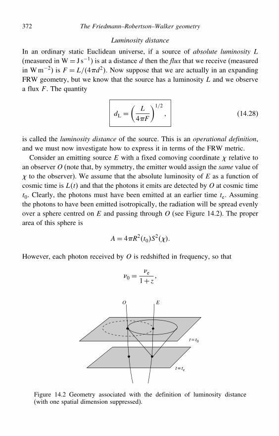
372 The Friedmann–Robertson–Walker geometry
Luminosity distance
In an ordinary static Euclidean universe, if a source of absolute luminosity L
(measured in W= J s−1) is at a distance d then the flux that we receive (measuredin Wm−2) is F = L/4d2. Now suppose that we are actually in an expandingFRW geometry, but we know that the source has a luminosity L and we observea flux F . The quantity
dL =(
L
4F
)1/2
(14.28)
is called the luminosity distance of the source. This is an operational definition,and we must now investigate how to express it in terms of the FRW metric.
Consider an emitting source E with a fixed comoving coordinate relative toan observer O (note that, by symmetry, the emitter would assign the same value of to the observer). We assume that the absolute luminosity of E as a function ofcosmic time is Lt and that the photons it emits are detected by O at cosmic timet0. Clearly, the photons must have been emitted at an earlier time te. Assumingthe photons to have been emitted isotropically, the radiation will be spread evenlyover a sphere centred on E and passing through O (see Figure 14.2). The properarea of this sphere is
A= 4R2t0S2
However, each photon received by O is redshifted in frequency, so that
0 =e
1+ z
t = te
t = t0
O E
Figure 14.2 Geometry associated with the definition of luminosity distance(with one spatial dimension suppressed).
14.11 Distances in the FRW geometry 373
and, moreover, the arrival rate of the photons is also reduced by the same factor.Thus, the observed flux at O is
Ft0=Lte
4 R0S2
11+ z2
The luminosity distance defined above is now evaluated as
dL = R0S1+ z (14.29)
This is an important quantity, which can be used practically, but note that itdepends on the time history of the scale factor through the dependence on .
Angular diameter distance
Another important distance measure is based upon the notion of the existence ofsome standard-length ‘rods’, whose angular diameter we can observe. Supposethat a source has proper diameter . Then, in Euclidean space, if it were at adistance d it would subtend an angular diameter =D/d. In an FRW geometry,we thus define the angular diameter distance to an object to be
dA =
(14.30)
This is again an operational definition, and we now investigate how to express itin terms of the FRW metric.
Suppose we have two radial null geodesics (light paths) meeting at the observerat time t0 with an angular separation , having been emitted at time te froma source of proper diameter at a fixed comoving coordinate (assuming,for simplicity, that the spatial axes are oriented so that = constant along thephoton paths); see Figure 14.3. To obtain a clearer view of the specification ofthe coordinates, we may look vertically down the worldline of O and define thecoordinates as in Figure 14.4. From the angular part of the FRW metric we have
= RteS
so that
dA = RteS= Rt0Rte
Rt0S= Rt0S
1+ z
Thus the angular diameter distance is given by
dA =R0S
1+ z (14.31)
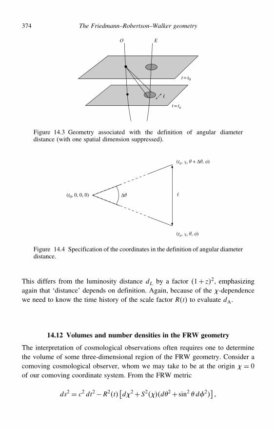
374 The Friedmann–Robertson–Walker geometry
t = t0
t = te
EO
Figure 14.3 Geometry associated with the definition of angular diameterdistance (with one spatial dimension suppressed).
(te, χ, θ + ∆θ, φ)
(te, χ, θ, φ)
(t0, 0, 0, 0) ∆θ
Figure 14.4 Specification of the coordinates in the definition of angular diameterdistance.
This differs from the luminosity distance dL by a factor 1+ z2, emphasizingagain that ‘distance’ depends on definition. Again, because of the -dependencewe need to know the time history of the scale factor Rt to evaluate dA.
14.12 Volumes and number densities in the FRW geometry
The interpretation of cosmological observations often requires one to determinethe volume of some three-dimensional region of the FRW geometry. Consider acomoving cosmological observer, whom we may take to be at the origin = 0of our comoving coordinate system. From the FRW metric
ds2 = c2 dt2−R2t[d2+S2d2+ sin2 d2
]
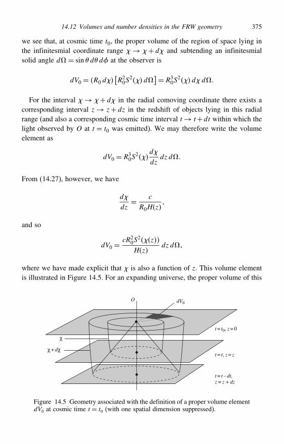
14.12 Volumes and number densities in the FRW geometry 375
we see that, at cosmic time t0, the proper volume of the region of space lying inthe infinitesmial coordinate range → +d and subtending an infinitesmialsolid angle d= sin dd at the observer is
dV0 = R0 d[R20S
2d]= R3
0S2d d
For the interval → +d in the radial comoving coordinate there exists acorresponding interval z→ z+dz in the redshift of objects lying in this radialrange (and also a corresponding cosmic time interval t→ t+dt within which thelight observed by O at t = t0 was emitted). We may therefore write the volumeelement as
dV0 = R30S
2d
dzdzd
From (14.27), however, we have
d
dz= c
R0Hz
and so
dV0 =cR2
0S2z
Hzdzd
where we have made explicit that is also a function of z. This volume elementis illustrated in Figure 14.5. For an expanding universe, the proper volume of this
O
t = t0, z = 0
t = t, z = z
t = t – dt,z = z + dz
dV0
χ
χ + dχ
Figure 14.5 Geometry associated with the definition of a proper volume elementdV0 at cosmic time t = t0 (with one spatial dimension suppressed).
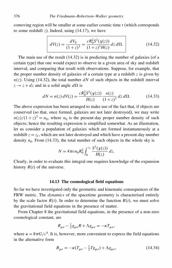
376 The Friedmann–Robertson–Walker geometry
comoving region will be smaller at some earlier cosmic time t (which correspondsto some redshift z). Indeed, using (14.17), we have
dVz= dV0
1+ z3= cR2
0S2z
1+ z3Hzdzd (14.32)
The main use of the result (14.32) is in predicting the number of galaxies (of acertain type) that one would expect to observe in a given area of sky and redshiftinterval, and comparing that result with observations. Suppose, for example, thatthe proper number density of galaxies of a certain type at a redshift z is given bynz. Using (14.32), the total number dN of such objects in the redshift intervalz→ z+dz and in a solid angle d is
dN = nzdVz= cR20S
2z
Hz
nz
1+ z3dzd (14.33)
The above expression has been arranged to make use of the fact that, if objects areconserved (so that, once formed, galaxies are not later destroyed), we may writenz/1+ z3 = n0, where n0 is the present-day proper number density of suchobjects; hence the resulting expression is simplified somewhat. As an illustration,let us consider a population of galaxies which are formed instantaneously at aredshift z= zf , which are not later destroyed and which have a present-day numberdensity n0. From (14.33), the total number of such objects in the whole sky is
N = 4cn0R20
∫ zf
0
S2z
Hzdz
Clearly, in order to evaluate this integral one requires knowledge of the expansionhistory Rt of the universe.
14.13 The cosmological field equations
So far we have investigated only the geometric and kinematic consequences of theFRW metric. The dynamics of the spacetime geometry is characterised entirelyby the scale factor Rt. In order to determine the function Rt, we must solvethe gravitational field equations in the presence of matter.
From Chapter 8 the gravitational field equations, in the presence of a non-zerocosmological constant, are
R− 12gR+$g =−&T
where &= 8G/c4. It is, however, more convenient to express the field equationsin the alternative form
R =−&T− 12Tg+$g (14.34)
14.13 The cosmological field equations 377
where T = T . In order to solve these equations, we clearly need a model for the
energy–momentum tensor of the matter that fills the universe. For simplicity, weshall grossly idealise the universe and model the matter by a simple macroscopicfluid, devoid of shear-viscous, bulk-viscous and heat-conductive properties. Thuswe assume a perfect fluid, which is characterised at each point by its proper density and the pressure p in the instantaneous rest frame. The energy–momentumtensor is given by
T =(+ p
c2
)uu−pg (14.35)
Since we are seeking solutions for a homogeneous and isotropic universe, thedensity and pressure p must be functions of cosmic time t alone.
We may perform the calculation in any coordinate system, but the algebra issimplified slightly by adopting the comoving coordinates x = t r , inwhich the FRW metric takes the form
ds2 = c2 dt2−R2t
[dr2
1−kr2+ r2d2+ sin2 d2
]
Thus the covariant components g of the metric are
g00 = c2 g11 =−R2t
1−kr2 g22 =−R2tr2 g33 =−R2tr2 sin2
Since the metric is diagonal, the contravariant components g are simply thereciprocals of the covariant components.
The connection is given in terms of the metric by
# = 1
2g#g+ g− g
from which it is straightforward to show that the only non-zero coefficients are
011 = RR/ c1−kr2 0
22 = RRr2/c 033 = RRr2 sin2 /c
101 = cR/R 1
11 = kr/1−kr2 033 = RRr2 sin2 /c
133 =−r1−kr2 sin2
202 = cR/R 2
12 = 1/r 233 = sin cos
303 = cR/R 3
13 = 1/r 323 = cot
where the dots denote differentiation with respect to cosmic time t. We nextsubstitute these expressions for the connection coefficients into the expression forthe Ricci tensor,
R = ## − #
#+
# #−
##
378 The Friedmann–Robertson–Walker geometry
After some tedious but straightforward algebra, we find that the off-diagonalcomponents of the Ricci tensor are zero and the diagonal components are given by
R00 = 3R/R
R11 = −RR+2R2+2c2kc−2/1−kr2
R22 = −RR+2R2+2c2kc−2r2
R33 = −RR+2R2+2c2kc−2r2 sin2
We must now turn our attention to the right-hand side of the field equa-tions (14.34). In our comoving coordinate system t r , the 4-velocity of thefluid is simply
u= 1000
which we can write as u = 0 . Thus the covariant components of the
4-velocity are
u = g0 = g0 = c20
so we can write the energy–momentum tensor (14.35) as
T = c2+pc200−pg
Moreover, since uu = c2, contraction of the energy–momentum tensor gives
T = T =
(+ p
c2
)c2−p = c2−3p
Hence we can write the terms on the right-hand side of the field equations (14.34)that depend on the energy–momentum as
T− 12Tg = c2+pc20
0− 1
2c2−pg
Including the cosmological-constant term, we find that the right-hand side of thefield equations (14.34) vanishes for = . The non-zero components read
−&T00− 12Tg00+$g00 = − 1
2&c2+3pc2+$c2
−&T11− 12Tg11+$g11 = −
[ 12&c
2−p+$]R2/1−kr2
−&T22− 12Tg22+$g22 = −
[ 12&c
2−p+$]R2r2
−&T33− 12Tg33+$g33 = −
[ 12&c
2−p+$]R2r2 sin2
Combining these expressions with those for the components of the Ricci tensor,we see that the three spatial field equations are equivalent, which is essentially
14.14 Equation of motion for the cosmological fluid 379
due to the homogeneity and isotropy of the FRW metric. Thus the gravitationalfield equations yield just the two independent equations,
3R/R = − 12&c
2+3pc2+$c2
RR+2R2+2c2k = [ 12&c
2−p+$]c2R2
Eliminating R from the second equation and remembering that &= 8G/c4, wefinally arrive at the cosmological field equations
R=−4G3
(+ 3p
c2
)R+ 1
3$c2R
R2 = 8G3
R2+ 13$c
2R2− c2k
(14.36)
These two differential equations determine the time evolution of the scale factorRt and are known as the Friedmann–Lemaître equations. In the case $= 0 theyare often called simply the Friedmann equations. We will discuss the solutionsto these equations in various cases in Chapter 15.
14.14 Equation of motion for the cosmological fluid
For any particular model of the universe, the two cosmological field equa-tions (14.36) are sufficient to determine Rt. Nevertheless, we can derive onefurther important equation (which is often useful in shortening calculations) fromthe fact that energy–momentum conservation requires
T = 0
From our discussion of a perfect fluid in Chapter 8, we know that this requirementleads to the relativistic equations of continuity and motion for the cosmologicalfluid. These equations read
u+ p
c2u
= 0 (14.37)(+ p
c2
)uu
=(g− uu
c2
)p (14.38)
The second equation is easily shown to be satisfied identically, since both sidesequal zero. This confirms that the fluid particles (galaxies) follow geodesics,which was to be expected since p is a function of t alone, and so there is nopressure gradient to push them off geodesics. The continuity equation (14.37) canbe written
pu+
(+ p
c2
)u
+ u
= 0
380 The Friedmann–Robertson–Walker geometry
Remembering that is a function of t alone, and with u = 0 , this reduces to
+(+ p
c2
) 3RR= 0 (14.39)
which expresses energy conservation. This equation can in fact be derived directlyfrom the field equations (14.36) by eliminating R. Thus, only two of the threeequations (14.36) and (14.39) are independent. One may use whichever twoequations are most convenient in any particular calculation.
Equation (14.39) can be simply rearranged into the useful alternative form
dR3
dt=−3pRR2
c2 (14.40)
Moreover, by transforming the derivative with respect to t to a derivative withrespect to R, one obtains a third useful form of the equation, namely
dR3
dR=−3pR2
c2 (14.41)
Finally, we note that the density and pressure of a fluid are related by itsequation of state. In cosmology, it is usual to assume that (each component of)the cosmological fluid has an equation of state of the form
p= wc2
where the equation-of-state parameter w is a constant (in the more exotic cosmo-logical models one sometimes allows w to be a function of cosmic time t, but weshall not consider such models here). The energy equation (14.41) can then bewritten
dR3
dR=−3wR2
This equation has the immediate solution
∝ R−31+w (14.42)
which gives the evolution of the density as a function of the scale factor Rt.Note that in general c2 is the energy density of the fluid. In particular w = 0for pressureless ‘dust’, w = 1
3 for radiation and w = −1 for the vacuum (if thecosmological constant $ = 0; see Section 8.7).
Exercises 381
14.15 Multiple-component cosmological fluid
Suppose that the cosmological fluid in fact consists of several distinct components(for example, matter, radiation and the vacuum) that do not interact except throughtheir mutual gravitation. Let us suppose further that each component can bemodelled as a perfect fluid, as discussed above.
The energy–momentum tensor of a multiple-component fluid is given simply by
T =∑iTi
where i labels the various fluid components. Since each component is modelledas a perfect fluid, we have
T =∑i
[(i+
pic
)uu−pig
]
=∑i
(i+
pic
)uu−
∑ipig
Thus, the multicomponent fluid can itself be modelled as a single perfect fluid with
=∑ii and p=∑
ipi (14.43)
which can be substituted directly into our cosmological field equations (14.36).4
Moreover, since we are assuming that the fluid components are non-interacting,conservation of energy and momentum requires that the condition
Ti = 0
holds separately for each component. Then each fluid will obey an energy equationof the form (14.39). Thus, if wi = pi/ic
2 then the density of each fluid evolvesindependently of the other components as
i ∝ R−31+wi (14.44)
Exercises
14.1 In an N -dimensional manifold, consider the tensor
Rijkl = Kgikgjl−gilgjk
whereK may be a function of position. Show that this tensor satisfies the symmetryproperties and the cyclic identity of the curvature tensor. Show that, in order tosatisfy the Bianchi identity, one requires K to be constant if N > 2.
4 Unfortunately, if the individual equation-of-state parameters wi are constants one cannot, in general, definea single effective equation-of-state parameter w = p/c2 that is also independent of cosmic time t.
382 The Friedmann–Robertson–Walker geometry
14.2 For a 3-space with a line element of the form
d#2 = Brdr2+ r2d2+ r2 sin2 d2
show that the non-zero components of the Ricci tensor are
Rrr =−1rB
dB
dr R =
1B−1− r
2B2
dB
dr R = R sin
2
Hence show that if the 3-space is maximally symmetric then Br must take theform
Br= 1A−Kr2
where A and K are constants.14.3 In a four-dimensional Euclidean space with ‘Cartesian’ coordinates wx y z, a
3-sphere of radius R is defined by w2+x2+ y2+ z2 = R2. Show that the metricon the surface of the 3-sphere can be written in the form
d#2 = R2[d2+ sin2 d2+ sin2 d2
]
Show that the total volume of the 3-sphere is V = 22R3.14.4 In a four-dimensional Minkowski space with ‘Cartesian’ coordinates wx y z,
a 3-hyperboloid is defined by w2−x2− y2+−z2 = R2. Show that the metric onthe surface of the 3-hyperboloid can be written in the form
d#2 = R2[d2+ sinh2 d2+ sin2 d2
]
Show that the total volume of the 3-hyperboloid is infinite.14.5 At cosmic time t1, a massive particle is shot out into an expanding FRW universe
with velocity v1 relative to comoving cosmological observers. At a later cosmictime t2 the particle has a velocity v2 with respect to comoving cosmologicalobservers. Show that, at any intermediate cosmic time t, the velocity of the particleas measured by a comoving cosmological observer is
vt= Rtd
dt
Hence show thatv2
v2
v1v1= Rt1
Rt2
where v = 1− v2/c2−1/2 and Rt is the scale factor at cosmic time t. Byconsidering the particle momentum, show that as v1 → c the photon redshiftformula is recovered.
14.6 In the limit z 1, show that the look-back time for a galaxy with redshift z is
t0− t =H−10 z−H−1
0
(1+ 1
2q0)z2+· · ·
Exercises 383
Show also that, in this limit, the variation of the Hubble parameter with redshiftis given by
Hz=H0 1+ 1+q0z−· · ·
14.7 In a spatially flat FRW geometry, show that the luminosity and angular diameterdistances to an object of redshift z are given, in the limit z 1, by
dL =c
H0
[z+ 1
2 1−q0z2+· · · ]
dA =c
H0
[z− 1
2 3+q0z2+· · · ]
Hence show that the angular diameter of a standard object can increase as z
increases. Do these results still hold in a spatially curved FRW geometry?14.8 In the FRW geometry, show that the look-back time to a nearby object at proper
distance d is
t0− t = d
c− H0d
2
2c2+· · ·
Hence show that the redshift to the object is
z= H0d
c+ 1+q0
2H2
0d2
c2+· · ·
14.9 The observed flux in the frequency range 1 2 received from some distantcomoving object is given by
Fobs1 2=∫ 2
1
fobsd
where fobsv is the observed flux density (in Wm−2 Hz−1) as a function offrequency. If fem is the emitted (or intrinsic) flux density of the object, showthat
fobs=fem1+ z
1+ z
where z is the redshift of the object. If fem∝ over a wide range of frequencies,show that
Fobs1 2= Kz Fem1 2
where the K-correction is given by Kz = 1+ z−1.14.10 The observed surface brightness (obs of an extended object observed in the
frequency range 1 2 is defined as the observed flux per unit solid angle. Thus,for a (small) circular object subtending an angular diameter we have
(obs =4Fobs1 2
2
384 The Friedmann–Robertson–Walker geometry
where Fobs1 2 is defined in Exercise 14.9. Show that (obs can be written as
(obs =4
Lem1 2
42Kz
1+ z4
where is the physical (projected) diameter of the object, Lem1 2 is theintrinsic luminosity of the object in the frequency range 1 2 and Kz is theK-correction.Note: The above result is independent of cosmological parameters. Moreover,setting aside the K-correction, the 1+ z−4-dependence means that the surfacebrightness of extended objects drops very rapidly with redshift, making the detec-tion of high-z objects difficult.
14.11 A commonly used distance measure in cosmology is the proper-motion distancedM defined by
dM =v
where v is the proper transverse velocity of (some part of) the object, which isassumed known from astrophysics, and is the corresponding observed angularvelocity. Show that
dM = 1+ zdA =dL
1+ z
where dA and dL are the angular-diameter distance and the luminosity distance tothe object respectively.
14.12 A certain population of galaxies undergoes a short ultra-luminous phase at redshiftz= z∗ that lasts for a proper time interval t. After this phase, such galaxies areneither created or destroyed. If z∗ 1, show that for a spatially flat universe thetotal number of such galaxies in the sky that are in this phase is given by
N = 4c3n0t
H20
[z∗ + 1
2 1−q0z2∗ + · · ·
]
where n0 is the present-day proper number density of these galaxies.14.13 In the comoving coordinates x= t r , the FRW metric takes the form
ds2 = c2 dt2−R2t
[dr2
1−kr2+ r2d2+ sin2 d2
]
Using the ‘Lagrangian’ method, or otherwise, calculate the corresponding connec-tion coefficients #
. Hence calculate the non-zero elements of the Riccitensor R.
14.14 In Newtonian cosmology, the universe is modelled as an infinite gas of density tthat is expanding in such a way that the relative recessional velocity of any twogas particles is vt=HtRt, where Ht= Rt/Rt and Rt is the separation
Exercises 385
of the particles at time t. Use Gauss’ law to determine the force on a particle ofmass m on the edge of an arbitrary spherical region, and hence show that
R=−4G3
R
By considering the total energy E of the above particle, show further that
R2 = 8G3
R2− c2k
where the constant k=−2E/mc2. Compare these Newtonian cosmological fieldequations with their general-relativistic counterparts.
14.15 Show that the relativistic equation of motion for the cosmological fluid is satisfiedidentically and that the relativistic equation of continuity takes the form
+(+ p
c2
) 3RR= 0
Show further that this equation may also be written in the forms
dR3
dt=−3pRR2
c2and
dR3
dR=−3pR2
c2
14.16 Use the cosmological field equations directly to derive the relativistic equation ofcontinuity for the cosmological fluid given in Exercise 14.15.
14.17 Consider a spherical comoving volume of the cosmological fluid whose surface isdefined by = constant. As the universe expands show that, for the infinitesimaltime interval t→ t+dt, the conservation of energy requires that
c2V = c2+dV +dV+pdV
where c2 and p are the energy density and pressure of the fluid respectively.Hence show that
d
dR=−31+w
R
where w = p/c2 and Rt is the scale factor of the universe. Show that thisequation has the solution ∝ R−31+w.
15
Cosmological models
In the previous chapter, we considered the geometric and kinematic properties ofthe Friedmann–Robertson–Walker (FRW) metric and derived the cosmologicalfield equations for the scale factor Rt. In this chapter, we will use the cosmo-logical field equations to determine the behaviour of the scale factor as a functionof cosmic time in various cosmological models.
15.1 Components of the cosmological fluid
In a general cosmological model, the universe is assumed to contain both matterand radiation. In addition, the cosmological constant $ is generally assumed to benon-zero. As discussed in Section 8.7, the modern interpretation of $ is in termsof the energy density of the vacuum, which may also be modelled as a perfectfluid (with a peculiar equation of state). Thus, one usually adopts the viewpointthat the cosmological fluid consists of three components, namely matter, radiationand the vacuum, each with a different equation of state. The total equivalent massdensity is simply the sum of the individual contributions,
t= mt+rt+$t (15.1)
where t is the cosmic time and we have adopted the commonly used cosmologicalnotation for the equivalent mass densities of matter, radiation and the vacuumrespectively. Moreover, we shall assume that these three components are non-interacting (see Section 14.13); although matter and radiation did interact in theearly universe, this is a reasonable approximation for most of its history.
As mentioned in Section 14.12, each component of the cosmological fluid ismodelled as a perfect fluid with an equation of state of the form
pi = wiic2
386
15.1 Components of the cosmological fluid 387
where the equation-of-state parameter wi is a constant (and i labels the compo-nent). In particular wi= 0 for pressureless ‘dust’, wi= 1
3 for radiation and wi=−1for the vacuum. In general, if wi is a constant then, requiring that the weak energycondition is satisfied (see Exercise 8.8) and that the local sound speed dp/d1/2
is less than c, one finds that wi must lie in the range −1 ≤ wi ≤ 1. We see thatthis is indeed the case for dust, radiation and the vacuum. We now discuss eachof these components in turn and conclude with a description of their relativecontributions to the total density as the universe evolves.
Matter
In general, matter in the universe may come in several different forms. In addi-tion to the normal baryonic matter of everyday experience (such as protons andneutrons), the universe may well contain more exotic forms of matter consistingof fundamental particles that lie beyond the ‘Standard Model’ of particle physics.Indeed, observations of the large-scale structure in the universe suggest that mostof the matter is in the form of non-baryonic dark matter, which interacts electro-magnetically only very weakly (and is hence invisible or ‘dark’). Moreover, darkmatter may itself come in different forms, such as cold dark matter (CDM) andhot dark matter (HDM), the naming of which is connected to whether the typicalenergy of the particles is non-relativistic or relativistic. We shall not pursue thisvery interesting subject any further here1 but merely note that the total matterdensity (at any particular cosmic time t) may be expressed as the sum of thebaryonic and dark matter contributions,
mt= bt+dmt
In the following discussion, we will not differentiate between different types ofmatter, since it is only the total matter density that determines how the scale factorRt evolves with cosmic time t. We shall also make the common assumption thatthe matter particles (in whatever form) have a thermal energy that is much lessthan their rest mass energy, and so the matter can be considered to be pressureless,i.e. dust. In this case the equation of state parameter is simply w= 0. Thus, from(14.44), if the matter has a present-day proper density of mt0≡ m0, its densityat some other cosmic time t is given by
mt= m0
[R0
Rt
]3or mz= m01+ z3
1 For a full discussion, see (for example) T. Padmanabhan, Structure Formation in the Universe, CambridgeUniversity Press, 1993.
388 Cosmological models
where in the second expression we have used (14.17) to write the density in termsof the redshift z. These expressions concur with our expectation for the behaviourof the space density of dust particles in an expanding universe.
Radiation
The term radiation naturally includes photons, but also other species with verysmall or zero rest masses, such that they move relativistically today. An exampleof the latter is neutrinos (which may in fact have a small non-zero rest mass). Thetotal equivalent mass density of radiation in the universe at some cosmic time t
may then be written as the sum of the photon and neutrino contributions:
rt= t+t
Once again, we will not differentiate between different types of radiation in oursubsequent discussion, since it is only the total energy density that determinesthe behaviour of the scale factor. For radiation, in general, we have w= 1
3 . Thus,from (14.44), if the total radiation in the universe has a present-day energy densityof r0c
2 then, at other cosmic times,
rt= r0
[R0
Rt
]4or rz= r01+ z4
In this case, the variation in the space density of photons (for example) again goesas 1+z3, but there is an additional factor 1+z resulting from the cosmologicalredshift of each photon.
It is worth noting that, to a very good approximation, the dominant contributionto the radiation energy density of the universe is due to the photons of thecosmic microwave background (CMB). This radiation is (to a very high degreeof accuracy) uniformly distributed throughout the universe and has a blackbodyform. For blackbody radiation, the number density of photons with frequenciesin the range +d is given by
nTd = 82
c3(eh/kT −1
) d (15.2)
where T is the ‘temperature’ of the radiation. Since the energy per unit frequencyis simply uT= nTh, the total equivalent mass density of the radiation is
rT=1c2
∫
0u d =
aT 4
c2
where a = 42k4B/603c3 is the reduced Stefan–Boltzmann constant. Obser-
vations show that the CMB is characterised by a present-day temperature
15.1 Components of the cosmological fluid 389
T0 = 2726K, which corresponds to a total present-day number density n0 ≈4×10⁸ m−3. It is easily shown that the CMB photon energy distribution retainsits general blackbody form as the universe expands. Thus, at any given cosmictime t, the temperature of the CMB radiation in the universe is given by
Tt= T0
[R0
Rt
]or Tz= T01+ z (15.3)
from which we see that the universe must have not only been denser in the past,but also ‘hotter’.
Vacuum
As mentioned above the vacuum can be modelled as a perfect fluid havingan equation of state p = −c2, so that the fluid has a negative pressure. Thiscorresponds to an equation of state parameter w = −1. Thus, from (14.44), wesee that at any cosmic time t, we have
$ = $0 =$c2
8G
Thus, the energy density of the vacuum always has the same constant value.
Relative contributions of the components
On combining the above results, we find that the variation in the total equivalentmass density (15.1) may be written as
t= m0
[R0
Rt
]3+r0
[R0
Rt
]4+$0 (15.4)
From this expression, we see that the relative contributions of matter, radiationand the vacuum to the total density vary as the universe evolves. The detailsclearly depend on the relative values of m0, r0 and $0. Typically, however,one would expect radiation to dominate the total density when Rt is small. Asthe universe expands, the radiation energy density dies away the most quicklyand matter becomes the dominant component. Finally, if the universe continuesto expand then the matter density also dies away and the vacuum ultimatelydominates the energy density. We conclude by noting that cosmologists oftendefine the normalised scale parameter
at≡ Rt
R0
in terms of which the above results are more compactly written, since a0 = 1 bydefinition. We shall make use of this parameter further in subsequent sections.
390 Cosmological models
15.2 Cosmological parameters
In our very simplified model of the universe discussed above, its entire historyis determined by only a handful of cosmological parameters. In particular, if onespecifies the values of the equivalent mass densities mt∗, rt∗ and $ atsome particular cosmic time t∗ then the value of each density, and hence the totaldensity, is determined at all other cosmic times t. Thus, specifying these quantitiesis sufficient to determine the scale factor Rt at all cosmic times. It is mostnatural to take t∗ to be the present-day cosmic time t0, and so the cosmologicalmodel is entirely fixed by specifying the three quantities
m0 r0 $0
It is, however, both convenient and common practice in cosmology to workinstead in terms of alternative dimensionless quantities, usually called densityparameters or simply densities, which are defined by
it≡8G3H2t
it (15.5)
where Ht is the Hubble parameter and the label i denotes ‘m’, ‘r’ or ‘$’. Itis worth noting that $t is, in general, a function of cosmic time t (unlike$, which is a constant). In terms of these new dimensionless parameters, thecosmological model may thus be fixed by specifying the values of the fourpresent-day quantities
H0 m0 r0 $0 (15.6)
A major goal of observational cosmology is therefore to determine these quantitiesfor our universe. Significant advances in the last decade mean that cosmologistsnow know these values to an accuracy of just a few per cent.2 We simply notehere that
H0 ≈ 70km s−1Mpc−1 m0 ≈ 03 r0 ≈ 5×10⁻⁵ $0 ≈ 07
(15.7)
where the units of H0 are those most commonly used in cosmology, in which1Mpc≡ 106 parsecs≈ 309×1022 m; in SI units, H0 ≈ 227×10−18 s−1. Perhapsmost astonishing is that the present-day energy density of the universe is domi-nated by the vacuum!
2 How these observational advances have been achieved is discussed in, for example, J. Peacock, CosmologicalPhysics, Cambridge University Press, 1999 or P. Coles & F. Lucchin, Cosmology: The Origin and Evolutionof Cosmic Structure (2nd edition), Wiley, 2002.
15.2 Cosmological parameters 391
We also note, for completeness, that cosmologists define further analogousdimensionless density parameters for the individual contributions to the matterand the radiation. For example, b, dm and are commonly used to denotethe dimensionless density of baryons, dark matter and neutrinos respectively. Forour universe, cosmological observations suggest the present-day values
b0 ≈ 005 dm0 ≈ 025 0 ≈ 0 (15.8)
noting, in particular, that only around one-sixth of the matter density is in the formof the familiar baryonic matter. Moreover, the majority of the baryonic matterseems not to reside in ordinary (hydrogen-burning) stars; the contribution of suchstars is only ∗ ≈ 0008. The values of the individual quantities (15.8) affect theastrophysical process occurring in the universe and have a profound influence on,for example, the formation of structure. For determining the overall expansionhistory of the universe, however, only the quantities (15.6) need be specified.
The reason for defining the densities (15.5) becomes clear when we rewritethe second of the cosmological field equations (14.36) in terms of them. Dividingthis equation through by R2 and noting that H = R/R, we obtain
1=m+r+$−c2k
H2R2 (15.9)
where, for notational simplicity, we have dropped the explicit time dependence ofthe variables. Indeed, it is also common practice to define the curvature densityparameter
kt=−c2k
H2tR2t (15.10)
so that, at all cosmic times t, we have the elegant relation
m+r+$+k = 1 (15.11)
It should be noted that, in cosmological models with positive spatial curvaturek = 1, the parameter k is negative. Moreover, if the cosmological constant$ is negative then so too is the vacuum density parameter $. This behaviourshould be contrasted with that of m and r, which are always positive.
From (15.9), we see that the values of m, r and $ determine the spatialcurvature of the universe in a simple fashion. We have three cases:
m+r+$ < 1 ⇔ negative spatial curvature k=−1 ⇔ ‘open’m+r+$ = 1 ⇔ zero spatial curvature k= 0 ⇔ ‘flat’m+r+$ > 1 ⇔ positive spatial curvature k= 1 ⇔ ‘closed’
392 Cosmological models
The above relations are valid at any cosmic time t but are most often applied tothe present day, t = t0. In particular, it is also clear from (15.9) that, althoughthe density parameters mr and $ are all, in general, functions of cosmictime t, their sum cannot change sign. Thus, the universe cannot evolve from oneform of the FRW geometry to another. We note that cosmologists often add tothe plethora of density parameters by also defining the total density parameter
≡m+r+$ = 1−k (15.12)
which is related to the total equivalent mass density (15.1) by = 8G/3H2.From (15.7), we see that for our universe 0 ≈ 1 or equivalently k0 ≈ 0, andit is therefore close to being spatially flat k= 0.
Finally, it is worth noting that, for any cosmological model to be spatiallyflat, one requires = 1 and it is common to describe the corresponding totalequivalent mass density as the critical density, which is given by
crit ≡3H2
8G
Hence, for any given value of the Hubble parameter, this expression gives the totalequivalent mass density required for the universe to be spatially flat. Since recentcosmological observations suggest that our universe is indeed close to spatiallyflat and, (15.7), that H0 ≈ 70km s−1Mpc−1, one finds that the present-day totalequivalent mass density in our universe is
crit0 =3H2
0
8G≈ 92×10−27 kg m−3
As mentioned above, it is thought that only around 30 per cent of this equivalentmass density is in the form of matter and only around 5 per cent in the form ofbaryonic matter. Nevertheless, it is worth noting that crit0 ≈ 55 protonsm−3,and so the critical density turns out to be extremely low by laboratory standards.3
15.3 The cosmological field equations
Since the cosmological model can be fixed by specifying the values of the quan-tities listed in (15.6), it is worthwhile rewriting the cosmological field equations(14.36) in terms of these parameters. Let us begin with the second field equation.Recalling that H = R/R, this may be written
H2 = 8G3
(∑ii
)− c2k
R2
3 The fact that this is a number of order unity is an accident of our choice of units!
15.4 General dynamical behaviour of the universe 393
where the label i includes matter, radiation and the vacuum. From (15.4), (15.5)and (15.10), we therefore find
H2 =H20
(m0 a
−3+r0 a−4+$0+k0 a
−2) (15.13)
where we have written the result in terms of the dimensionless scale parametera= R/R0. It should be remembered that k0 = 1−m0−r0−$0 and maybe considered merely as a convenient shorthand. It is also worth noting that, sincea= R/R0 = 1+z−1, equation (15.13) immediately yields an expression for theHubble parameter Hz as a function of redshift z.
We now turn to the first cosmological field equation in (14.36). Multiplyingthis equation through by R/R2 and again noting that H = R/R, we have
RR
R2=−4G
3H2
∑ii1+3wi
where the label i once more includes matter, radiation and the vacuum. The left-hand side is equal to minus the deceleration parameter q defined in (14.19). Thus,substituting the appropriate value of wi for each component and using (15.5), onefinds the neat relation
q = 12m+2r−2$ (15.14)
If desired, one can easily write this equation explicitly in terms of the present-dayvalues of the density parameters by using the result (15.13) and the relation
i =i0
(H0
H
)2
a−31+wi
which holds generally for matter, radiation and the vacuum.
15.4 General dynamical behaviour of the universe
The cosmological field equations (15.13) and (15.14) allow us to determine thegeneral dynamical behaviour and the spatial geometry of the universe for anygiven set of values for the parameters m0, r0 and $0. The observations(15.7) suggest that the present-day value of the radiation density r0 is signifi-cantly smaller than the matter and vacuum densities. It is therefore a reasonableapproximation to neglectr0 and parameterise a universe like our own in terms ofjustm0 and$0 (and H0, which is irrelevant for our discussion in this section).
Figure 15.1 presents a summary of the properties of FRW universes dominatedby matter and vacuum energy (known as Lemaitre models) as a function of
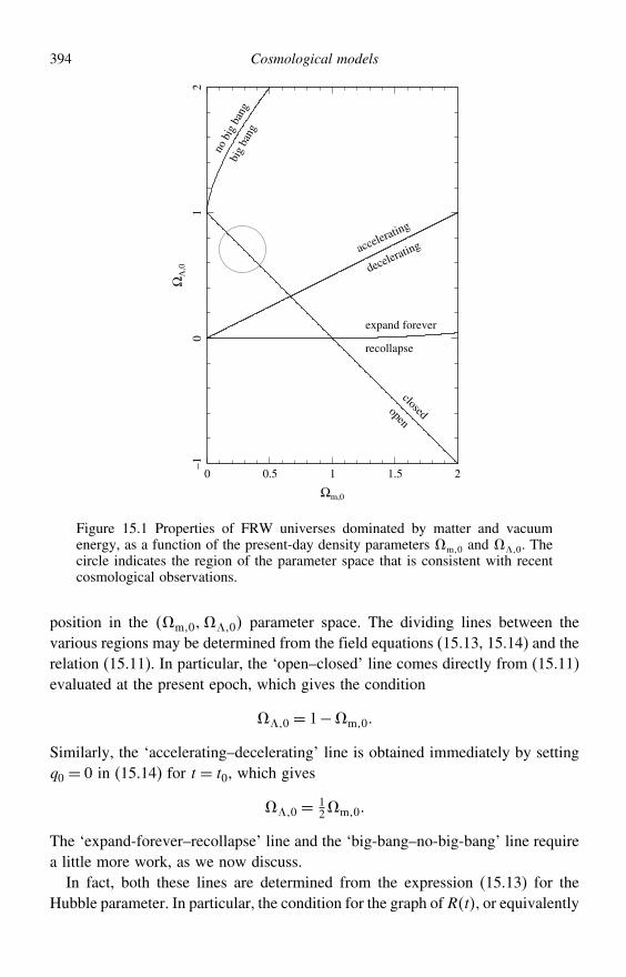
394 Cosmological models
accelerating
decelerating
closedopenno
big
ban
gbi
g ba
ng
expand forever
recollapse
0
–10
12
0.5 1
Ωm,0
ΩΛ
,0
1.5 2
Figure 15.1 Properties of FRW universes dominated by matter and vacuumenergy, as a function of the present-day density parameters m0 and $0. Thecircle indicates the region of the parameter space that is consistent with recentcosmological observations.
position in the m0$0 parameter space. The dividing lines between thevarious regions may be determined from the field equations (15.13, 15.14) and therelation (15.11). In particular, the ‘open–closed’ line comes directly from (15.11)evaluated at the present epoch, which gives the condition
$0 = 1−m0
Similarly, the ‘accelerating–decelerating’ line is obtained immediately by settingq0 = 0 in (15.14) for t = t0, which gives
$0 = 12m0
The ‘expand-forever–recollapse’ line and the ‘big-bang–no-big-bang’ line requirea little more work, as we now discuss.
In fact, both these lines are determined from the expression (15.13) for theHubble parameter. In particular, the condition for the graph of Rt, or equivalently
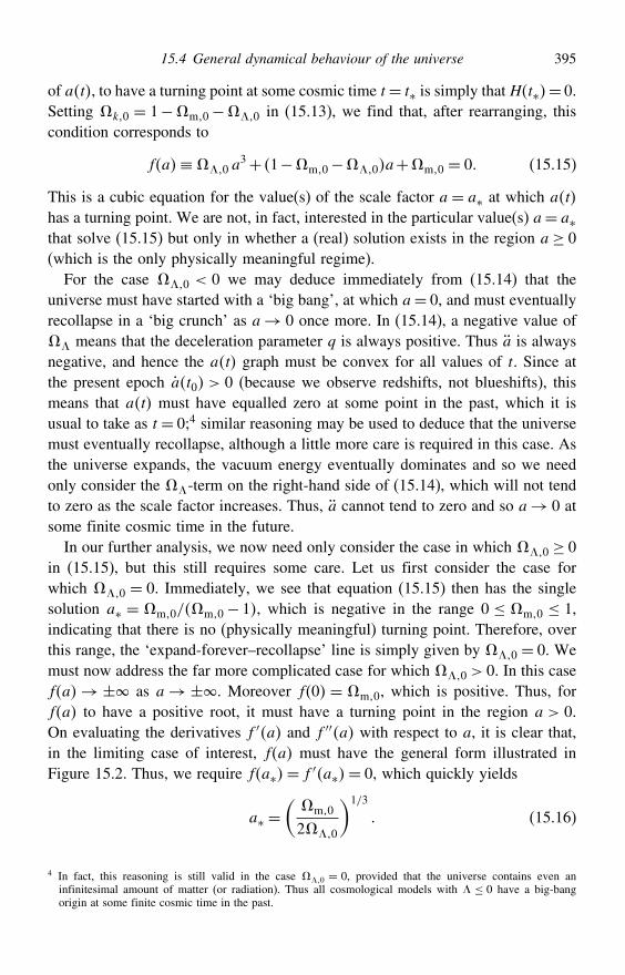
15.4 General dynamical behaviour of the universe 395
of at, to have a turning point at some cosmic time t= t∗ is simply thatHt∗= 0.Setting k0 = 1−m0−$0 in (15.13), we find that, after rearranging, thiscondition corresponds to
fa≡$0 a3+ 1−m0−$0a+m0 = 0 (15.15)
This is a cubic equation for the value(s) of the scale factor a= a∗ at which at
has a turning point. We are not, in fact, interested in the particular value(s) a= a∗that solve (15.15) but only in whether a (real) solution exists in the region a≥ 0(which is the only physically meaningful regime).
For the case $0 < 0 we may deduce immediately from (15.14) that theuniverse must have started with a ‘big bang’, at which a= 0, and must eventuallyrecollapse in a ‘big crunch’ as a→ 0 once more. In (15.14), a negative value of$ means that the deceleration parameter q is always positive. Thus a is alwaysnegative, and hence the at graph must be convex for all values of t. Since atthe present epoch at0 > 0 (because we observe redshifts, not blueshifts), thismeans that at must have equalled zero at some point in the past, which it isusual to take as t = 0;4 similar reasoning may be used to deduce that the universemust eventually recollapse, although a little more care is required in this case. Asthe universe expands, the vacuum energy eventually dominates and so we needonly consider the $-term on the right-hand side of (15.14), which will not tendto zero as the scale factor increases. Thus, a cannot tend to zero and so a→ 0 atsome finite cosmic time in the future.
In our further analysis, we now need only consider the case in which $0 ≥ 0in (15.15), but this still requires some care. Let us first consider the case forwhich $0 = 0. Immediately, we see that equation (15.15) then has the singlesolution a∗ = m0/m0− 1, which is negative in the range 0 ≤ m0 ≤ 1,indicating that there is no (physically meaningful) turning point. Therefore, overthis range, the ‘expand-forever–recollapse’ line is simply given by $0 = 0. Wemust now address the far more complicated case for which $0 > 0. In this casefa→± as a→±. Moreover f0 = m0, which is positive. Thus, forfa to have a positive root, it must have a turning point in the region a > 0.On evaluating the derivatives f ′a and f ′′a with respect to a, it is clear that,in the limiting case of interest, fa must have the general form illustrated inFigure 15.2. Thus, we require fa∗= f ′a∗= 0, which quickly yields
a∗ =(m0
2$0
)1/3
(15.16)
4 In fact, this reasoning is still valid in the case $0 = 0, provided that the universe contains even aninfinitesimal amount of matter (or radiation). Thus all cosmological models with $ ≤ 0 have a big-bangorigin at some finite cosmic time in the past.
396 Cosmological models
a
f (a)
Ωm,0
–a* a*
Figure 15.2 The limiting form of the cubic fa defined in (15.15) for $0 > 0.
On substituting this expression back into (15.15) one then obtains a separate cubicequation for $0, given by
41−m0−$03+272
m0$0 = 0 (15.17)
By introducing the variable x = $0/4m01/3, this equation quickly
reduces to
x3− 3x4+ m0−1
4m0= 0
which is amenable to analysis using the standard formulae for finding the rootsof a cubic. In particular, rewriting the resulting roots in terms of $0, one findsthe following three cases:
• 0<m0 ≤ 12 , one positive root at
$0 = 4m0 cosh3
[13cosh−1
(1−m0
m0
)] (15.18)
• 12 <m0 ≤ 1, one positive root at
$0 = 4m0 cos3
[13cos−1
(1−m0
m0
)] (15.19)
• m0 > 1, two positive roots, the larger given by (15.19) and the smaller by
$0 = 4m0 cos3
[13cos−1
(1−m0
m0
)+ 4
3
] (15.20)
15.5 Evolution of the scale factor 397
Moreover, from (15.16), one easily finds that a∗ < 1 for (15.18, 15.19), whereasa∗ > 1 for (15.20). Since the universe is expanding, a∗ < 1 corresponds to aturning point in the past (i.e. no big bang), whereas a∗ > 1 corresponds to aturning point in the future (i.e. recollapse).
The resulting lines, plotted in Figure 15.1, show some interesting features. Inparticular, we note that when $0 = 0 there is a direct correspondence betweenthe geometry of the universe and its eventual fate. In this case, open universesexpand forever, whereas closed universes recollapse. This correspondence nolonger holds in the presence of a non-zero cosmological constant, in which caseany combination of spatial geometry and eventual fate is possible. It is alsoworth noting that the region of the m0$0-plane consistent with recentcosmological observations is centred on the spatially flat model (0.3,0.7) andexcludes the possibility of a zero cosmological constant at high significance.These observations also show the expansion of the universe to be accelerating.They also require the universe to have started at a big bang at some finite cosmictime in the past and to expand forever in the future.
15.5 Evolution of the scale factor
So far, we have considered only the limiting behaviour of the (normalised)scale factor at for different values of the cosmological parameters; this wassummarised in Figure 15.1. We now discuss how to find the form of the at-curve at all cosmic times, for a given set of (present-day) cosmological parametervalues. This behaviour is entirely determined by the cosmological field equation(15.13). Remembering that H = a/a, this may be written as(
da
dt
)2
=H20
(m0 a
−1+r0 a−2+$0a
2+1−m0−r0−$0
)
(15.21)Instead of working directly in terms of the cosmic time t, it is more convenientto introduce the new dimensionless variable
t =H0t− t0 (15.22)
which measures cosmic time relative to the present epoch in units of the ‘Hubbletime’ H−1
0 . In terms of this new variable, (15.21) becomes
(da
dt
)2
=m0 a−1+r0 a
−2+$0a2+1−m0−r0−$0 (15.23)
There exist some special cases, where m0, r0 and $0 take on particularsimple values, for which equation (15.23) can be solved analytically; we will
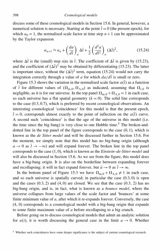
398 Cosmological models
discuss some of these cosmological models in Section 15.6. In general, however, anumerical solution is necessary. Starting at the point t= 0 (the present epoch), forwhich a0 = 1, the normalised scale factor at time step n+1 can be approximatedby the Taylor expansion
an+1 ≈ an+(da
dt
)n
t+ 12
(d2a
dt2
)n
t2 (15.24)
where t is the (small) step size in t. The coefficient of t is given by (15.23),and the coefficient of t2 may be obtained by differentiating (15.23). The latteris important since, without the t2 term, equation (15.24) would not carry theintegration correctly through a value of a for which da/dt is small or zero.
Figure 15.3 shows the variation in the normalised scale factor at as a functionof t for different values of m0$0 as indicated, assuming that r0 isnegligible, as it is for our universe. In the top panel m0+$0 = 1 in each case,so each universe has a flat spatial geometry k = 0. The solid line correspondsto the case (0.3, 0.7), which is preferred by recent cosmological observations. Aninteresting cosmological ‘coincidence’ for this model is that the present epoch,t = 0, corresponds almost exactly to the point of inflection on the at curve.A second such ‘coincidence’ is that the age of the universe in this model (i.e.the time since the big bang) is very close to one Hubble time.5 The broken-and-dotted line in the top panel of the figure corresponds to the case (0, 1), which isknown as the de Sitter model and will be discussed further in Section 15.6. Forthe moment, we simply note that this model has no big-bang origin (althougha→ 0 as t→−) and will expand forever. The broken line in the top panelcorresponds to the case (1, 0), which is known as the Einstein–de-Sitter model andwill also be discussed in Section 15.6. As we see from the figure, this model doeshave a big-bang origin. It is also on the borderline between expanding foreverand recollapsing; it will in fact expand forever, but a→ 0 as t→.
In the bottom panel of Figure 15.3 we have m0+$0 = 1 in each case,and so each universe is spatially curved; in particular the case (0.3, 0) is openand the cases (0.3, 2) and (4, 0) are closed. We see that the case (0.3, 2) has nobig-bang origin, and is, in fact, what is known as a bounce model, where theuniverse collapses from large values of the scale factor and ‘bounces’ at somefinite minimum value of a, after which it re-expands forever. Conversely, the case(4, 0) corresponds to a cosmological model with a big-bang origin that expandsto some finite maximum value of a before recollapsing to a big crunch.
Before going on to discuss cosmological models that admit an analytic solutionfor at, it is worth discussing the general case in the limit a→ 0. Whether
5 Whether such coincidences have some deeper significance is the subject of current cosmological research.
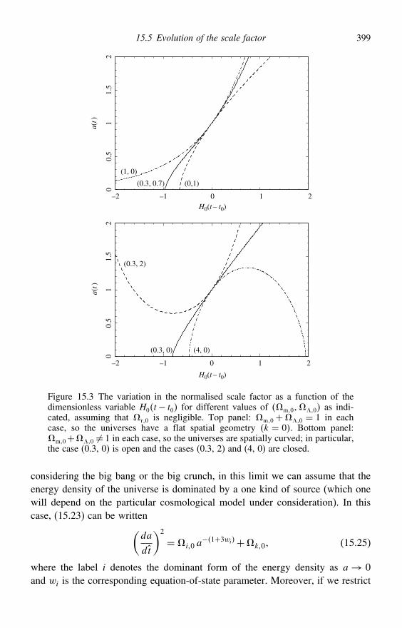
15.5 Evolution of the scale factor 399
H0(t – t0)
a(t)
–2
00.
51
1.5
2
a(t)
00.
51
1.5
2
–1 0 1 2
H0(t – t0)
–2 –1 0 1 2
(1, 0)
(0,1)(0.3, 0.7)
(0.3, 2)
(4, 0)(0.3, 0)
Figure 15.3 The variation in the normalised scale factor as a function of thedimensionless variable H0t− t0 for different values of m0$0 as indi-cated, assuming that r0 is negligible. Top panel: m0 +$0 = 1 in eachcase, so the universes have a flat spatial geometry k = 0. Bottom panel:m0+$0 = 1 in each case, so the universes are spatially curved; in particular,the case (0.3, 0) is open and the cases (0.3, 2) and (4, 0) are closed.
considering the big bang or the big crunch, in this limit we can assume that theenergy density of the universe is dominated by a one kind of source (which onewill depend on the particular cosmological model under consideration). In thiscase, (15.23) can be written(
da
dt
)2
=i0 a−1+3wi+k0 (15.25)
where the label i denotes the dominant form of the energy density as a→ 0and wi is the corresponding equation-of-state parameter. Moreover, if we restrict
400 Cosmological models
our attention to the (realistic) case, in which i denotes either dust wi = 0 orradiation wi = 1
3, then the first term on the right-hand side of (15.25) dominatesas a→ 0, so we can neglect the curvature density k0. In this case, (15.25) canbe immediately integrated to give
at=±[321+wi
√i0
]2/ 31+wi
t− t∗2/ 31+wi (15.26)
where t∗ is the value of t at which a= 0 and the plus and minus signs correspondto the big bang and big crunch respectively. From (15.25), we also note thatda/dt→ as a→ 0. Thus, we conclude that the at-graph meets the t-axis atright angles.
15.6 Analytical cosmological models
Although in the general case the evolution of the (normalised) scale factor atmust be determined numerically, there exist a number of special cases, corre-sponding to particular values of the cosmological parameters m0, r0 and$0, for which equation (15.23) can be solved analytically. We now discusssome of these analytical cosmological models, all of which have inherited specialnames that are widely used in cosmology. In this section, we will work in termsof the cosmic time t directly, rather than the dimensionless variable t definedin (15.22).
The Friedmann models
Cosmological models with a zero cosmological constant (and, strictly, a non-zeromatter or radiation density) are known as the Friedmann models. As noted inSection 15.4, all Friedmann models have a big-bang origin at a finite cosmic timein the past. Moreover, it is possible to place a strict upper limit on the age of theuniverse in such models. Since the at-curve is everywhere convex, it is clearfrom Figure 15.4 that it crosses the t-axis at a time that is closer to the presenttime t = t0 than the time at which the tangent to the point t0 a0 reaches thet-axis (note that a0 = 1). Clearly, the point where the tangent meets the t-axis isthe point at which at would have been zero for a = constant and a = 0. Thetime elapsed from that point to the present epoch is simply at0/at0 = H−1
0 .Thus, in Friedmann models, the age of the universe must be less than the Hubbletime:
t0 <H−10
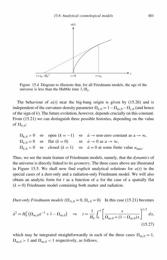
15.6 Analytical cosmological models 401
t
a(t)
t = t0 – H0 t = 0 t = t0–1
Figure 15.4 Diagram to illustrate that, for all Friedmann models, the age of theuniverse is less than the Hubble time 1/H0.
The behaviour of at near the big-bang origin is given by (15.26) and isindependent of the curvature density parameterk0= 1−m0−r0 (and henceof the sign of k). The future evolution, however, depends crucially on this constant.From (15.21) we can distinguish three possible histories, depending on the valueof k0:
k0 > 0 ⇔ open k=−1 ⇔ a→ non-zero constant as a→
k0 = 0 ⇔ flat k= 0 ⇔ a→ 0 as a→
k0 < 0 ⇔ closed k= 1 ⇔ a= 0 at some finite value amax
Thus, we see the main feature of Friedmann models, namely, that the dynamics ofthe universe is directly linked to its geometry. The three cases above are illustratedin Figure 15.5. We shall now find explicit analytical solutions for at in thespecial cases of a dust-only and a radiation-only Friedmann model. We will alsoobtain an analytic form for t as a function of a for the case of a spatially flatk= 0 Friedmann model containing both matter and radiation.
Dust-only Friedmann models $0 = 0r0 = 0 In this case (15.21) becomes
a2 =H20
(m0a
−1+1−m0
) ⇒ t = 1H0
∫ a
0
[x
m0+ 1−m0x
]1/2dx
(15.27)
which may be integrated straightforwardly in each of the three cases m0 = 1,m0 > 1 and m0 < 1 respectively, as follows.
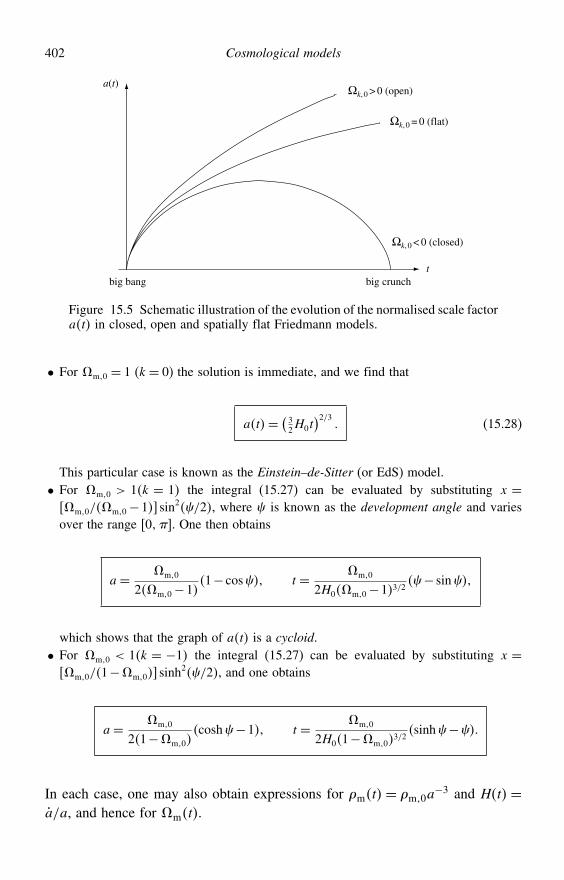
402 Cosmological models
t
Ωk, 0 > 0 (open)
Ωk, 0 = 0 (flat)
Ωk, 0 < 0 (closed)
big bang
a(t)
big crunch
Figure 15.5 Schematic illustration of the evolution of the normalised scale factorat in closed, open and spatially flat Friedmann models.
• For m0 = 1 (k= 0) the solution is immediate, and we find that
at= ( 32H0t)2/3
(15.28)
This particular case is known as the Einstein–de-Sitter (or EdS) model.• For m0 > 1k = 1 the integral (15.27) can be evaluated by substituting x = m0/m0−1 sin2/2, where is known as the development angle and variesover the range 0. One then obtains
a= m0
2m0−11− cos t = m0
2H0m0−13/2− sin
which shows that the graph of at is a cycloid.• For m0 < 1k = −1 the integral (15.27) can be evaluated by substituting x = m0/1−m0 sinh
2/2, and one obtains
a= m0
21−m0cosh−1 t = m0
2H01−m03/2
sinh−
In each case, one may also obtain expressions for mt = m0a−3 and Ht =
a/a, and hence for mt.
15.6 Analytical cosmological models 403
Radiation-only Friedmann models $0 = 0m0 = 0 In this case (15.21)becomes
a2 =H20
(r0a
−2+1−r0
) ⇒ t = 1H0
∫ a
0
x√r0+ 1−r0x
2dx
(15.29)
which may again be integrated straightforwardly for r0 = 1, r0 > 1 andr0 < 1 respectively.
• For r0 = 1 (k= 0) the solution is again immediate, and we find that
at= 2H0t1/2
• Forr0 < 1k=−1 andr0 > 1k= 1 the integral (15.29) can be evaluatedby inspection to give
at=(2H0
1/2r0 t
)1/2(1+ 1−r0
21/2r0
H0t
)1/2
In each case, one may again obtain expressions for rt= m0a−3 and Ht=
a/a, and hence for rt.
Spatially flat Friedmann models $0= 0,m0+r0= 1 In this case (15.21)becomes
a2 =H20
(m0a
−1+r0a−2) ⇒ t = 1
H0
∫ a
0
x√m0x+r0
dx
(15.30)
which may be straightforwardly integrating by substituting y =m0x+r0 toobtain
H0t =2
32m0
[m0a+r0
1/2m0a−2r0+23/2r0
]
Unfortunately, this expression cannot be easily inverted to give at. Nevertheless,it is simple to show that the above expression becomes 2
3a3/2 for a matter-only
model and 12a
2 for a radiation-only model, and therefore agrees with our earlierresults.
404 Cosmological models
The Lemaitre models
The Lemaitre models are a generalisation of the Friedmann models in which thecosmological constant is non-zero. In particular, we will focus here on matter-only models (r0 = 0), although our discussion is easily modified for radiation-only models, and can be extended to include models containing both matter andradiation. The general dynamical properties of Lemaitre models with r0 = 0were discussed in detail in Section 15.4, with particular focus on their limitingbehaviour. We concentrate here on determining the generic form of the at-curvefor models of this type that have a big-bang origin and will expand forever.We begin by considering the general case of arbitrary spatial curvature and thenspecialise to the spatially flat case. A model of the latter sort appears to providea reasonable description of our own universe, if one neglects its radiation energydensity.
Matter-only Lemaitre models with arbitrary spatial curvature r0 = 0 In thiscase the cosmological field equation (15.13) reads
a2 =H20
(m0a
−1+$0a2+k0
) (15.31)
where k0 = 1−m0−$0. Obtaining explicit formulae giving, for example,the scale factor as a function of time is in general quite complicated, since theintegrals turn out to involve elliptic functions,6 which are unfamiliar to mostphysicists these days. Nevertheless, we see that for small a the first term on theright-hand side dominates and the equation is easily integrated. Thus, after startingfrom a big-bang origin at t = 0, the at-curve at first increases as
at=(32H0
√m0 t
)2/3for small t
which agrees with our earlier result (15.26). As the universe expands, however,the matter energy density decreases and the vacuum energy eventually dominates.Thus, for large t (and hence large a), the second term on the right-hand side of(15.31) dominates. Once again the equation is then easily integrated to give
at∝ exp(H0
√$0 t
)for large t
6 See e.g. M. Abramowitz & I. A. Stegun, Handbook of Mathematical Physics, Dover, 1972.
15.6 Analytical cosmological models 405
From the above limiting behaviour at small and large t, it is clear that theuniverse must, at some point, make a transition from a decelerating to an accel-erating phase. This occurs when a= 0, at which point the at-curve has a pointof inflection. Differentiating (15.31), we find that
a= 12H
20
(2$0a−m0a
−2) (15.32)
From this result, we may verify immediately that at early cosmic times (when a
is small) we have a < 0, and so the expansion is decelerating. As the universeexpands, the deceleration gradually decreases until a changes sign, after which theexpansion accelerates ever more rapidly. We see that the value of the normalisedscale factor at which the point of inflection (a= 0) occurs is given by
a∗ =(m0
2$0
)1/3
(15.33)
It is, in fact, possible to obtain an approximate analytic expression for thenormalised scale factor at in the vicinity of the point of inflection. To do this,we must first obtain an approximate form for the cosmological field equation(15.31) in the vicinity of this point. Denoting the cosmic time at the point ofinflection by t∗, we may perform separate Taylor expansions of a and a2 aboutt = t∗ to obtain
a≈ a∗ + a∗t− t∗ and a2 ≈ a2∗ + a∗...a∗t− t∗2
where, for notational convenience, we have written a∗ ≡ at∗, a∗ ≡ at∗, etc.Using the first expression to subtitute for t− t∗2 in the second, we obtain
a2 ≈ a2∗ +...a∗a−a∗2
a∗ (15.34)
Differentiating (15.32) one easily obtains an expression for...a . Then, substituting
(15.33) into the resulting expression, and into (15.31), one finds that (15.34)becomes
a2 ≈H20
[k0+3$0a
2∗ +3$0a−a∗2
]
This equation can now be integrated analytically and has the solution
at= a∗ +a∗[1+ 1
3k0
( 14$0
2m0
)−1/3]1/2sinh
[H03$0
1/2t− t∗]
(15.35)
An interesting property of this type of model is that in the case of positivespatial curvature (k = 1), for which k0 < 0, there is a ‘coasting period’ in the
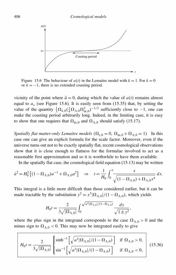
406 Cosmological models
t
Coasting period
a*
a(t)
Figure 15.6 The behaviour of at in the Lemaitre model with k= 1. For k= 0or k=−1, there is no extended coasting period.
vicinity of the point where a= 0, during which the value of at remains almostequal to a∗ (see Figure 15.6). It is easily seen from (15.35) that, by setting thevalue of the quantity 1
3k014$0
2m0
−1/3 sufficiently close to −1, one canmake the coasting period arbitrarily long. Indeed, in the limiting case, it is easyto show that one requires that m0 and $0 should satisfy (15.17).
Spatially flat matter-only Lemaitre models r0 = 0 m0+$0 = 1 In thiscase one can give an explicit formula for the scale factor. Moreover, even if theuniverse turns out not to be exactly spatially flat, recent cosmological observationsshow that it is close enough to flatness for the formulae involved to act as areasonable first approximation and so it is worthwhile to have them available.
In the spatially flat case, the cosmological field equation (15.13) may be written
a2=H20
[1−$0a
−1+$0a2] ⇒ t= 1
H0
∫ a
0
x√1−$0+$0x
4dx
This integral is a little more difficult than those considered earlier, but it can bemade tractable by the substitution y2 = x3$0/1−$0, which yields
H0t =2
3√$0
∫ √a3$0/1−$0
0
dy√1±y2
where the plus sign in the integrand corresponds to the case $0 > 0 and theminus sign to $0 < 0. This may now be integrated easily to give
H0t =2
3√$0
⎧⎪⎨⎪⎩sinh−1
[√a3$0/1−$0
]if $0 > 0
sin−1[√
a3$0/1−$0]
if $0 < 0(15.36)
15.6 Analytical cosmological models 407
which may be inverted to give at in each case. One can also obtain analyticexpressions for Ht and mt (see Exercise 15.24) and thus for mt and$t.
The de Sitter model
The de Sitter model is a particular special case of a Lemaitre model definedby the cosmological parameters m0 = 0, r0 = 0 and $0 = 1. This modelis therefore spatially flat (k = 0) but is not a true cosmological model in thestrictest sense, since it assumes that the matter and radiation densities are zero.Nevertheless, it is interesting in its own right both for historical reasons andbecause of its close connection with the theory of inflation (see Section 16.1).
For the de Sitter model, the cosmological field equation (15.13) reads(a
a
)2
=H20
which immediate tells us that the Hubble parameter Ht is a constant and thenormalised scale factor increases exponentially as
at= exp H0t− t0= exp[√
$/3ct− t0]
where, in the second equality, we have expressed the solution in terms of thecosmological constant $. Thus, the de Sitter model has no big-bang singularityat a finite time in the past.
Einstein’s static universe
All the cosmological models that we have constructed so far are evolving cosmolo-gies. We know now, of course, that the universe is expanding and so there is noconflict with the field equations. Nevertheless, it is interesting historically to lookat Einstein’s static model of the universe. Einstein derived his field equationswell before the discovery of the expansion of the universe and he was worriedthat he could not find static cosmological solutions. He therefore introduced thecosmological constant with the sole purpose of constructing static solutions.
For $ > 0, we seek a solution to the field equations in which the universe isstatic, i.e. a = a = 0. In this case, the Hubble parameter H is zero always, andso the dimensional densities in (15.5) are formally infinite. It is more convenienttherefore to work with the field equations in their original forms (14.36). We seeimmediately that we require
4Gm0 =$c2 = c2k
R20
408 Cosmological models
In fact, the first equality can be more succinctly written as m0 = 2$0. Since$ is positive we thus require k = 1, and so the universe has positive spatialcurvature.
How well did Einstein’s static universe fit with cosmological observations ofthe time? The mean matter density of the universe is still a matter of great debate,but recent cosmological observations suggest that
m0 ≈ 3×10⁻²⁷ kgm−3
In Einstein’s time, this value was estimated only to within about two ordersof magnitude. Nevertheless, adopting the above value of m0 we find that thescale factor is R0 ≈ 2×1026 m ≈ 6000Mpc, which is more than sufficient for theclosed spatial geometry to be large enough to encompass the observable universe.Also $= 1/R2
0 = 25×10−53 m−2, which is small enough to evade the limits on$ from Solar System experiments $ ≤ 10−46 m−2. Thus the Einstein staticuniverse was not immediately and obviously wrong.
However, aside from the fact that the model disagreed with later observationsindicating an expanding universe, it has the theoretically undesirable feature ofbeing unstable. The cosmological constant must be fine-tuned to match the densityof the universe. Thus, if we add or subtract one proton from this universe, orconvert some matter into radiation, we will disturb the finely tuned balancebetween gravity and the cosmological constant and the universe will begin toexpand or contract.
15.7 Look-back time and the age of the universe
Since the cosmological model may be fixed by specifying the values of the four(present-day) cosmological parameters H0, m0r0 and $0, it is possible touse these quantities to determine other useful derived cosmological parameters.In this section we consider the look-back time and the age of the universe.
In Chapter 14, we showed that if a comoving particle (galaxy) emitted a photonat cosmic time t that is received by an observer at t= t0 then the ‘look-back time’t0− t is given as a function of the photon’s redshift by
t0− t =∫ z
0
dz
1+ zHz (15.37)
From the cosmological field equation (15.13), on noting that a=R/R0= 1+z−1we obtain the useful result
H2z=H20
[m01+ z3+r01+ z4+$0+k01+ z2
] (15.38)
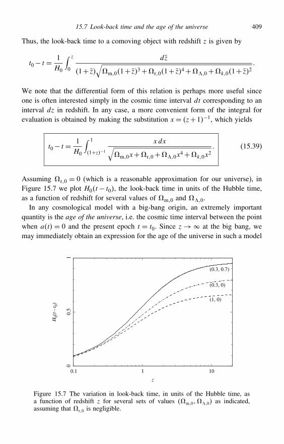
15.7 Look-back time and the age of the universe 409
Thus, the look-back time to a comoving object with redshift z is given by
t0− t = 1H0
∫ z
0
dz
1+ z√m01+ z3+r01+ z4+$0+k01+ z2
We note that the differential form of this relation is perhaps more useful sinceone is often interested simply in the cosmic time interval dt corresponding to aninterval dz in redshift. In any case, a more convenient form of the integral forevaluation is obtained by making the substitution x = z+1−1, which yields
t0− t = 1H0
∫ 1
1+z−1xdx√
m0x+r0+$0x4+k0x
2 (15.39)
Assuming r0 = 0 (which is a reasonable approximation for our universe), inFigure 15.7 we plot H0t− t0, the look-back time in units of the Hubble time,as a function of redshift for several values of m0 and $0.
In any cosmological model with a big-bang origin, an extremely importantquantity is the age of the universe, i.e. the cosmic time interval between the pointwhen at = 0 and the present epoch t = t0. Since z→ at the big bang, wemay immediately obtain an expression for the age of the universe in such a model
0.1
00.
51
1
z
10
(0.3, 0.7)
(1, 0)
(0.3, 0)
H0(
t–t 0
)
Figure 15.7 The variation in look-back time, in units of the Hubble time, asa function of redshift z for several sets of values m0$0 as indicated,assuming that r0 is negligible.
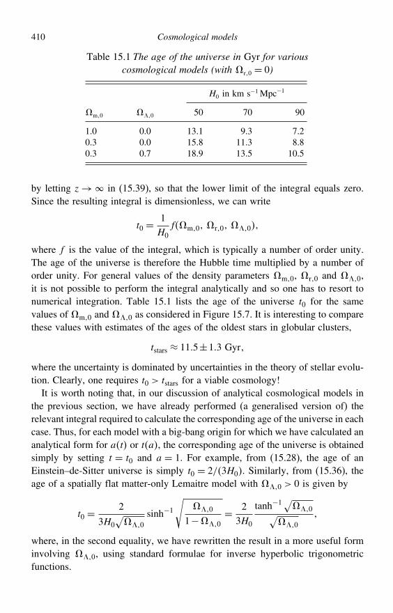
410 Cosmological models
Table 15.1 The age of the universe in Gyr for variouscosmological models (with r0 = 0)
H0 in km s−1 Mpc−1
m0 $0 50 70 90
1.0 0.0 13.1 9.3 7.20.3 0.0 15.8 11.3 8.80.3 0.7 18.9 13.5 10.5
by letting z→ in (15.39), so that the lower limit of the integral equals zero.Since the resulting integral is dimensionless, we can write
t0 =1H0
fm0 r0 $0
where f is the value of the integral, which is typically a number of order unity.The age of the universe is therefore the Hubble time multiplied by a number oforder unity. For general values of the density parameters m0, r0 and $0,it is not possible to perform the integral analytically and so one has to resort tonumerical integration. Table 15.1 lists the age of the universe t0 for the samevalues of m0 and $0 as considered in Figure 15.7. It is interesting to comparethese values with estimates of the ages of the oldest stars in globular clusters,
tstars ≈ 115±13 Gyr
where the uncertainty is dominated by uncertainties in the theory of stellar evolu-tion. Clearly, one requires t0 > tstars for a viable cosmology!It is worth noting that, in our discussion of analytical cosmological models in
the previous section, we have already performed (a generalised version of) therelevant integral required to calculate the corresponding age of the universe in eachcase. Thus, for each model with a big-bang origin for which we have calculated ananalytical form for at or ta, the corresponding age of the universe is obtainedsimply by setting t = t0 and a = 1. For example, from (15.28), the age of anEinstein–de-Sitter universe is simply t0 = 2/3H0. Similarly, from (15.36), theage of a spatially flat matter-only Lemaitre model with $0 > 0 is given by
t0 =2
3H0√$0
sinh−1√
$0
1−$0= 2
3H0
tanh−1√$0√
$0
where, in the second equality, we have rewritten the result in a more useful forminvolving $0, using standard formulae for inverse hyperbolic trigonometricfunctions.
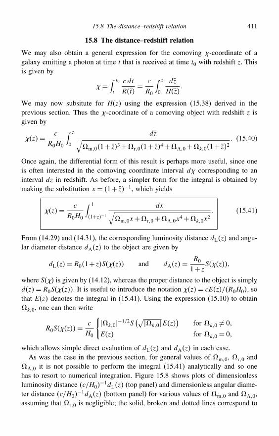
15.8 The distance–redshift relation 411
15.8 The distance–redshift relation
We may also obtain a general expression for the comoving -coordinate of agalaxy emitting a photon at time t that is received at time t0 with redshift z. Thisis given by
=∫ t0
t
c dt
Rt= c
R0
∫ z
0
dz
Hz
We may now subsitute for Hz using the expression (15.38) derived in theprevious section. Thus the -coordinate of a comoving object with redshift z isgiven by
z= c
R0H0
∫ z
0
dz√m01+ z3+r01+ z4+$0+k01+ z2
(15.40)
Once again, the differential form of this result is perhaps more useful, since oneis often interested in the comoving coordinate interval d corresponding to aninterval dz in redshift. As before, a simpler form for the integral is obtained bymaking the substitution x = 1+ z−1, which yields
z= c
R0H0
∫ 1
1+z−1dx√
m0x+r0+$0x4+k0x
2 (15.41)
From (14.29) and (14.31), the corresponding luminosity distance dLz and angu-lar diameter distance dAz to the object are given by
dLz= R01+ zSz and dAz=R0
1+ zSz
where S is given by (14.12), whereas the proper distance to the object is simplydz= R0Sz. It is useful to introduce the notation z= cEz/R0H0, sothat Ez denotes the integral in (15.41). Using the expression (15.10) to obtaink0, one can then write
R0Sz=c
H0
k0−1/2S
(√k0Ez)
for k0 = 0
Ez for k0 = 0
which allows simple direct evaluation of dLz and dAz in each case.As was the case in the previous section, for general values of m0, r0 and
$0 it is not possible to perform the integral (15.41) analytically and so onehas to resort to numerical integration. Figure 15.8 shows plots of dimensionlessluminosity distance c/H0
−1dLz (top panel) and dimensionless angular diame-ter distance c/H0
−1dAz (bottom panel) for various values of m0 and $0,assuming that r0 is negligible; the solid, broken and dotted lines correspond to
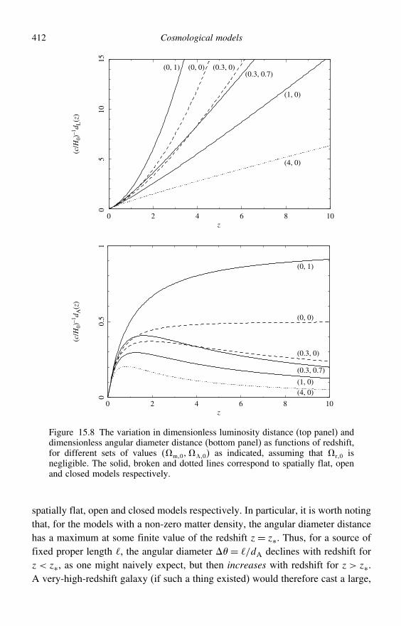
412 Cosmological models
00.
5
(c/H
0)–1
d A(z
)
10
510
(c/H
0)–1
d L(z
)
15
z0 2 4 6 8 10
z0 2 4 6 8 10
(4, 0)(1, 0)
(0.3, 0.7)
(0, 0)
(0, 1)
(0.3, 0)
(1, 0)
(0.3, 0.7)(0.3, 0)(0, 0)(0, 1)
(4, 0)
Figure 15.8 The variation in dimensionless luminosity distance (top panel) anddimensionless angular diameter distance (bottom panel) as functions of redshift,for different sets of values m0$0 as indicated, assuming that r0 isnegligible. The solid, broken and dotted lines correspond to spatially flat, openand closed models respectively.
spatially flat, open and closed models respectively. In particular, it is worth notingthat, for the models with a non-zero matter density, the angular diameter distancehas a maximum at some finite value of the redshift z= z∗. Thus, for a source offixed proper length , the angular diameter = /dA declines with redshift forz < z∗, as one might naively expect, but then increases with redshift for z > z∗.A very-high-redshift galaxy (if such a thing existed) would therefore cast a large,
15.9 The volume–redshift relation 413
but dim, ghostly image on the sky. The physical reason for this is that the lightfrom a distant object was emitted when the universe was much younger than it isnow – the object was close to us when the light was emitted. This, coupled withgravitational focussing of the light rays by the intervening matter in the universe,means that the galaxy looks big!
The integral (15.41) can, in fact, be evaluated analytically in some simple cases.As an example, consider the Einstein–de-Sitter (EdS) model (m0 = 1, r0 = 0,$0 = 0). In this case, we find that
z= c
R0H0
∫ 1
1+z−1dx√x= 2c
R0H0
[1− 1+ z−1/2
]
Thus, the luminosity distance in the EdS model is given as a function of z by
dLz=2cH0
1+ z[1− 1+ z−1/2
]
and the angular diameter distance by
dAz=2cH0
11+ z
[1− 1+ z−1/2
]
Note that, in this case, dAz has a maximum at a redshift z= 5/4.The relations between redshift and luminosity distance (angular diameter
distance), form the basis of observational tests of the geometry of the universe. Allone needs is a standard candle (for application of the luminosity-distance–redshiftrelation) or a standard ruler (for application of the angular-diameter-distance–redshift relation). Comparison with the predicted relations shown in Figure 15.8can then fix the values of m0 and $0. Unfortunately, standard candles andstandard rulers are hard to find in the universe! Nevertheless, in recent yearsthere has been remarkable progress, using distant Type Ia supernovae as standardcandles and anisotropies in the cosmic microwave background radiation as astandard ruler. The results of these observations suggest that we live in a spatiallyflat universe with m0 ≈ 03 and $0 ≈ 07.
15.9 The volume–redshift relation
In Section 14.10 we found that, at the present cosmic time t0, the proper volumeof the region of space lying in the infinitesmial coordinate range → +d andsubtending an infinitesmial solid angle d= sin dd at the observer is
dV0 =cR2
0S2z
Hzdzd (15.42)
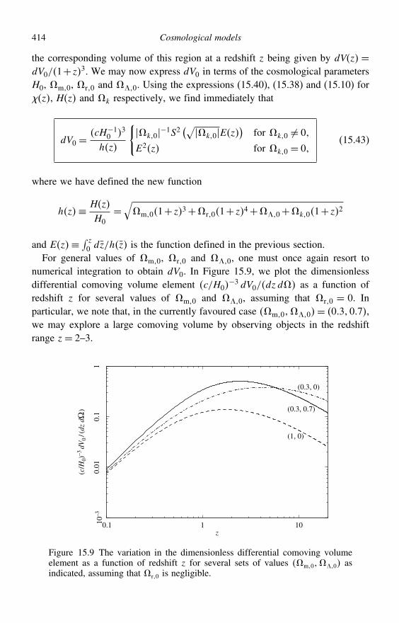
414 Cosmological models
the corresponding volume of this region at a redshift z being given by dVz =dV0/1+z3. We may now express dV0 in terms of the cosmological parametersH0, m0, r0 and $0. Using the expressions (15.40), (15.38) and (15.10) forz, Hz and k respectively, we find immediately that
dV0 =cH−1
0 3
hz
k0−1S2
(√k0Ez)
for k0 = 0
E2z for k0 = 0(15.43)
where we have defined the new function
hz≡ Hz
H0=√m01+ z3+r01+ z4+$0+k01+ z2
and Ez≡ ∫ z0 dz/hz is the function defined in the previous section.
For general values of m0, r0 and $0, one must once again resort tonumerical integration to obtain dV0. In Figure 15.9, we plot the dimensionlessdifferential comoving volume element c/H0
−3 dV0/dzd as a function ofredshift z for several values of m0 and $0, assuming that r0 = 0. Inparticular, we note that, in the currently favoured case m0$0= 0307,we may explore a large comoving volume by observing objects in the redshiftrange z= 2–3.
z0.1
10.
10.
0110
–3
1 10
(c/H
0)–3
dV0
/(dz
dΩ
)
(0.3, 0)
(0.3, 0.7)
(1, 0)
Figure 15.9 The variation in the dimensionless differential comoving volumeelement as a function of redshift z for several sets of values m0$0 asindicated, assuming that r0 is negligible.
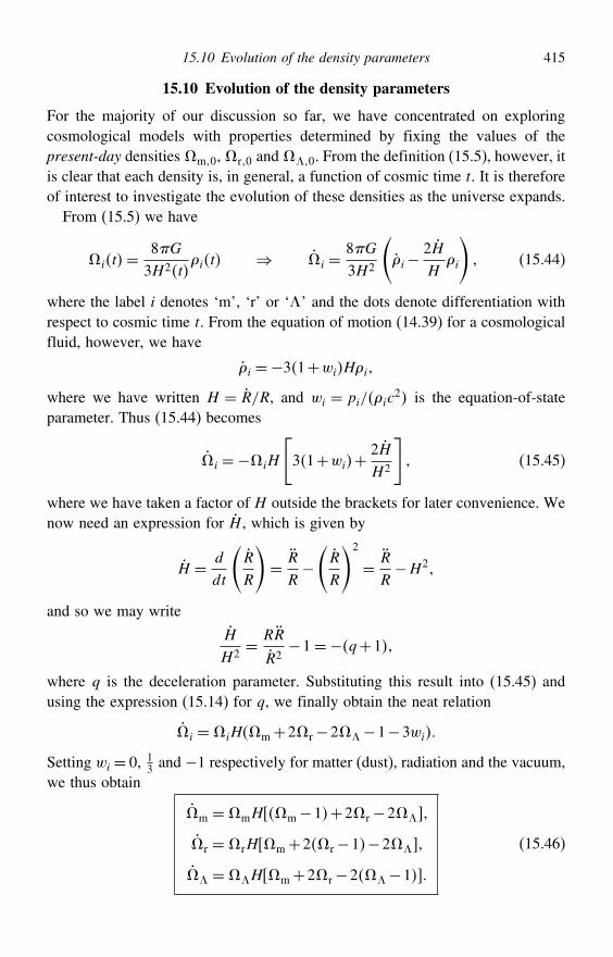
15.10 Evolution of the density parameters 415
15.10 Evolution of the density parameters
For the majority of our discussion so far, we have concentrated on exploringcosmological models with properties determined by fixing the values of thepresent-day densitiesm0,r0 and$0. From the definition (15.5), however, itis clear that each density is, in general, a function of cosmic time t. It is thereforeof interest to investigate the evolution of these densities as the universe expands.
From (15.5) we have
it=8G3H2t
it ⇒ i =8G3H2
(i−
2HH
i
) (15.44)
where the label i denotes ‘m’, ‘r’ or ‘$’ and the dots denote differentiation withrespect to cosmic time t. From the equation of motion (14.39) for a cosmologicalfluid, however, we have
i =−31+wiHi
where we have written H = R/R, and wi = pi/ic2 is the equation-of-state
parameter. Thus (15.44) becomes
i =−iH
[31+wi+
2HH2
] (15.45)
where we have taken a factor of H outside the brackets for later convenience. Wenow need an expression for H , which is given by
H = d
dt
(R
R
)= R
R−(R
R
)2
= R
R−H2
and so we may write
H
H2= RR
R2−1=−q+1
where q is the deceleration parameter. Substituting this result into (15.45) andusing the expression (15.14) for q, we finally obtain the neat relation
i =iHm+2r−2$−1−3wi
Setting wi = 0, 13 and −1 respectively for matter (dust), radiation and the vacuum,
we thus obtain
m =mH m−1+2r−2$
r =rH m+2r−1−2$
$ =$H m+2r−2$−1
(15.46)
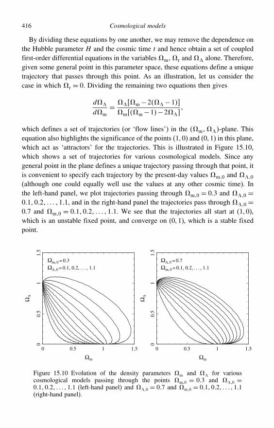
416 Cosmological models
By dividing these equations by one another, we may remove the dependence onthe Hubble parameter H and the cosmic time t and hence obtain a set of coupledfirst-order differential equations in the variablesm,r and$ alone. Therefore,given some general point in this parameter space, these equations define a uniquetrajectory that passes through this point. As an illustration, let us consider thecase in which r = 0. Dividing the remaining two equations then gives
d$
dm= $ m−2$−1
m m−1−2$
which defines a set of trajectories (or ‘flow lines’) in the m$-plane. Thisequation also highlights the significance of the points (1, 0) and (0, 1) in this plane,which act as ‘attractors’ for the trajectories. This is illustrated in Figure 15.10,which shows a set of trajectories for various cosmological models. Since anygeneral point in the plane defines a unique trajectory passing through that point, itis convenient to specify each trajectory by the present-day values m0 and $0
(although one could equally well use the values at any other cosmic time). Inthe left-hand panel, we plot trajectories passing through m0 = 03 and $0 =0102 11, and in the right-hand panel the trajectories pass through $0 =07 and m0 = 0102 11. We see that the trajectories all start at (1, 0),which is an unstable fixed point, and converge on (0, 1), which is a stable fixedpoint.
ΩΛ, 0 = 0.7
Ωm,0 = 0.1, 0.2, . . . , 1.1
Ωm,0 = 0.3
ΩΛ, 0 = 0.1, 0.2, . . . , 1.1
0
00.
51
1.5
00.
51
1.5
0.5 1 1.50 0.5 1 1.5
ΩΛ
ΩΛ
ΩmΩm
Figure 15.10 Evolution of the density parameters m and $ for variouscosmological models passing through the points m0 = 03 and $0 =0102 11 (left-hand panel) and $0 = 07 and m0 = 0102 11(right-hand panel).
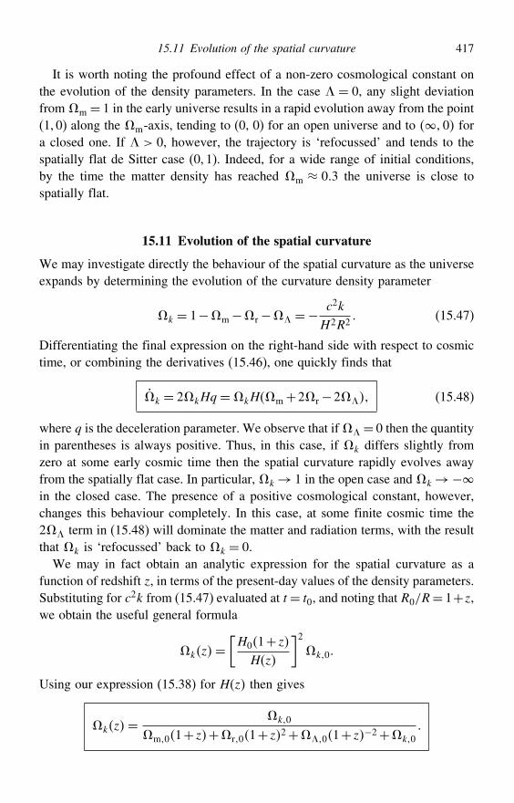
15.11 Evolution of the spatial curvature 417
It is worth noting the profound effect of a non-zero cosmological constant onthe evolution of the density parameters. In the case $ = 0, any slight deviationfromm = 1 in the early universe results in a rapid evolution away from the point(1, 0) along the m-axis, tending to (0, 0) for an open universe and to 0 fora closed one. If $ > 0, however, the trajectory is ‘refocussed’ and tends to thespatially flat de Sitter case (0, 1). Indeed, for a wide range of initial conditions,by the time the matter density has reached m ≈ 03 the universe is close tospatially flat.
15.11 Evolution of the spatial curvature
We may investigate directly the behaviour of the spatial curvature as the universeexpands by determining the evolution of the curvature density parameter
k = 1−m−r−$ =−c2k
H2R2 (15.47)
Differentiating the final expression on the right-hand side with respect to cosmictime, or combining the derivatives (15.46), one quickly finds that
k = 2kHq =kHm+2r−2$ (15.48)
where q is the deceleration parameter. We observe that if$= 0 then the quantityin parentheses is always positive. Thus, in this case, if k differs slightly fromzero at some early cosmic time then the spatial curvature rapidly evolves awayfrom the spatially flat case. In particular, k→ 1 in the open case and k→−in the closed case. The presence of a positive cosmological constant, however,changes this behaviour completely. In this case, at some finite cosmic time the2$ term in (15.48) will dominate the matter and radiation terms, with the resultthat k is ‘refocussed’ back to k = 0.
We may in fact obtain an analytic expression for the spatial curvature as afunction of redshift z, in terms of the present-day values of the density parameters.Substituting for c2k from (15.47) evaluated at t= t0, and noting that R0/R= 1+z,we obtain the useful general formula
kz=[H01+ z
Hz
]2k0
Using our expression (15.38) for Hz then gives
kz=k0
m01+ z+r01+ z2+$01+ z−2+k0
418 Cosmological models
In particular, we see that (apart from models with only vacuum energy), even ifthe present-day value k0 differs greatly from zero, at very high redshift (i.e.in the distant past) kz must have differed by only a tiny amount from zero.Since today we measure the value k0 to be (conservatively) in the range −05to 0.5, this means that at very early epochs k must have been very finely tunedto near zero. This tuning of the initial conditions of the expansion is called theflatness problem and has no solution within standard cosmological models. Fromour above discussion, however, the presence of a positive cosmological constantgoes some way to explaining why the universe is close to spatially flat at thepresent epoch.
15.12 The particle horizon, event horizon and Hubble distance
Thus far, we have considered the evolution of the entire spatial part of theFRW geometry. It is, however, interesting to consider the extent of the region‘accessible’ (via light signals) to some comoving observer at a given cosmictime t.
Particle horizon
Let us consider a comoving observer O situated (without loss of generality) at = 0. Suppose further that a second comoving observer E has coordinate 1 andemits a photon at cosmic time t1, which reaches O at time t. Assuming light tobe the fastest possible signal, the only signals emitted at time t1 that O receivesby the time t are from radial coordinates < 1.
The comoving coordinate 1 of the emitter E is determined by
1 = c∫ t
t1
dt
Rt (15.49)
If the integral on the right-hand side diverges as t1→ 0 then 1 can be made aslarge as we please by taking t1 sufficiently small. Thus, in this case, in principleit is possible to receive signals emitted at sufficiently early epochs from anycomoving particle (such as a typical galaxy). If, however, the integral convergesas t1→ 0 then 1 can never exceed a certain value for a given t. In this case ourvision of the universe is limited by a particle horizon. At any given cosmic timet, the -coordinate of the particle horizon is given by
pt= c∫ t
0
dt
Rt= c
∫ Rt
0
dR
RR (15.50)
where in the second equality we have rewritten the expression as an integral overR. The corresponding proper distance to the particle horizon is dpt=Rtpt.
15.12 The particle horizon, event horizon and Hubble distance 419
We see that expression (15.50) will be finite if RR∼ R with < 1, which isequivalent to the condition R < 0. Hence, any universe for which the expansionhas been continually decelerating up to the cosmic time t will have a finite particlehorizon at that time. Clearly, this includes all the Friedmann models that wediscussed earlier, but particle horizons also occur in other cosmological models,for example in the spatially flat Lemaitre model with m0 ≈ 03 and $0 ≈ 07that seems to provide a reasonable description of our universe.
On differentiating (15.50) with respect to t, we have dp/dt= c/Rt, which isalways greater than zero. Thus, the particle horizon of a comoving observer growsas the cosmic time t increases, and so parts of the universe that were not in viewpreviously must gradually come into view. This does not mean, however, that agalaxy that was not visible at one instant suddenly appears in the sky a momentlater! To understand this, we note that if the universe has a big-bang origin thenwe have Rt1→ 0 as t1 → 0, and so z→. Thus, the particle horizon at anygiven cosmic time is the surface of infinite redshift, beyond which we cannot see.If the particle horizon grew to encompass a galaxy, the galaxy would thereforeappear at first with an infinite redshift, which would gradually reduce as morecosmic time passed. Hence the galaxy would not simply ‘pop’ into view.7
In fact, we can obtain explicit expressions for the particle horizon in somecosmological models. For example, a matter-dominated model at early epochsobeys Rt/R0 = t/t0
2/3, whereas a radiation-dominated model at early epochsobeys Rt/R0 = t/t0
1/2. Substituting these expressions into (15.50) gives theproper distance to the particle horizon at cosmic time t as
dpt= 3ct (matter-dominated) dpt= 2ct (radiation-dominated)
These proper distances are larger than ct because the universe has expanded whilethe photon has been travelling. Alternatively, if one has an analytic expressionfor z for some cosmological model then the corresponding expression for pmay be obtained simply by letting z→.
The existence of particle horizons for the common cosmological models illus-trates the horizon problem, i.e. how do vastly separated regions display thesame physical characteristics (e.g. the nearly uniform temperature of the cosmicmicrowave background) when, according to standard cosmological models, theseregions could never have been in causal contact? This problem, like the flatnessproblem, is a serious challenge to standard cosmology that can only be resolvedby invoking the theory of inflation (see Chapter 16).
7 In practice, our view of the universe is not limited by our particle horizon but by the epoch of recombination,which occurred at zrec ≈ 1500 (long before the formation of any galaxies). Prior to this epoch, the universewas ionised and photons were frequently scattered by the free electrons, whereas after this point electrons andprotons (and neutrons) combined to form atoms and the photons were able to propagate freely. This surfaceof last scattering is therefore the effective limit of our observable universe.
420 Cosmological models
The horizon problem can be illustrated by a simple example. Consider a galaxyat a proper distance of 109 light years away from us. Since the age of the universeis ∼ 15× 1010 years, there has been sufficient time to exchange about 15 lightsignals with the galaxy. At earlier times, when the scale factor R was smaller,everything was closer together and so we might have naively expected that thiswould improve causal contact. In a continuously decelerating universe, however,it makes the problem worse. At, for example, the epoch of recombination (whenthe cosmic microwave background photons were emitted) the redshift z wasapproximately 1000, so Rtrec/R0 ≈ 10−3 and the proper distance to the ‘galaxy’is 106 light years.8 If we assume, for simplicity, that after trec the expansionfollowed a matter-dominated Einstein–de-Sitter universe, then(
trect0
)2/3
= Rrec
R0= 10−3
and so trec = 15×1055 years. However, assuming that prior to trec the expansionfollowed a radiation-dominated Einstein–de-Sitter model, the proper distance tothe particle (causal) horizon is 2ctrec = 3× 1055 light years. Thus, by trec ‘we’could not have exchanged even one light signal with the other ‘galaxy’.
Event horizon
Although our particle horizon grows as the cosmic time t increases, in somecosmological models there could be events that we may never see (or, conversely,never influence). Returning to our expression (15.49), we see that if the integralon the right-hand side diverges as t→ (or the time at which R equals zeroagain), then it will be possible to receive light signals from any event. However,if the integral instead converges for large t then, for light signals emitted at t1, wewill only ever receive those from events for which the -coordinate is less than
et1= c∫ tmax
t1
dt
Rt
where tmax is either infinity or the time of the big crunch (i.e. Rtmax= 0). Thisis called the event horizon. By symmetry, et0 is the maximum -coordinatethat can be reached by a light signal sent by us today.
Hubble distance
From our discussion in Section 15.7, the elapsed cosmic time t since the bigbang is, in general, of the order H−1t, which is known as the Hubble time and
8 In reality the galaxy would not yet have formed, but this does not affect the main point of the argument.
Exercises 421
provides a characteristic time scale for the expansion of the universe. In a similarway, at a cosmic time t one can define the Hubble distance
dHt= cH−1t
which provides a characteristic length scale for the universe. We may also definethe comoving Hubble distance
Ht=dHt
Rt= c
HtRt= c
Rt (15.51)
where in the last equality we have used the fact that H = R/R. The aboveexpression simply gives the -coordinate corresponding to the Hubble distance.
The Hubble distance dHt corresponds to the typical length scale (at cosmictime t) over which physical processes in the universe operate coherently. It is alsothe length scale at which general-relativistic effects become important; indeed,on length scales much less than dHt, Newtonian theory is often sufficient todescribe the effects of gravitation. From our discussion above, we further notethat the proper distance to the particle horizon for standard cosmological modelsis typically
dpt∼ ct ∼ cH−1t
Thus, we see that the particle horizon in such cases is of the same order as theHubble distance. As a result, the Hubble distance is often described simply as the‘horizon’. It should be noted, however, that the particle horizon and the Hubbledistance are distinct quantities, which may differ by many orders of magnitude ininflationary cosmologies, which we discuss in the next chapter. In particular, wenote that the particle horizon at time t depends on the entire expansion history ofthe universe to that point, whereas the Hubble distance is defined instantaneouslyat t. Moreover, once an object lies within an observer’s particle horizon it remainsso. On the contrary, an object can be within an observer’s Hubble distance at onetime, lie outside it at some later time and even come back within it at a still laterepoch.
Exercises
15.1 For blackbody radiation, the number density of photons with frequencies in therange +d is given by
nTd = 82
c3 eh/kT −1d (E15.1)
where T is the ‘temperature’ of the radiation. By conserving the total numberof photons, show that the photon energy distribution of the cosmic microwave
422 Cosmological models
background (CMB) radiation retains its general blackbody form as the universeexpands. Show further that the total number density n of photons is
nT= 0244(2kBThc
)3
Hence show that the present-day number density of CMB photons in the universe isn0 ≈ 4×10⁸ m−3, and compare this with the present-day number density of protons.How does this ratio vary with cosmic time?
Hint:∫ 0
x2
ex−1dx = 02442.
15.2 Suppose that the present-day energy densities of radiation and matter (in the formof dust) are rt0c
2 and mt0c2 respectively. Show that the energy densities of
the two components were equal at a redshift zeq given by
1+ zeq =mt0
rt0
What assumptions underlie this result? Hence show that
1+ zeq =3c2m0H
20
8GaT 40
where a is the reduced Stefan–Boltzmann constant and T0 is the present-day temper-ature of the cosmic microwave background. Show that for our universe zeq ≈ 5000.What was the temperature of the CMB radiation at this epoch?
15.3 Show that in the early, radiation-dominated, phase of the universe, the temperatureT of the radiation satisfies the equation(
T
T
)2
= 8GaT 4
3
where the dot denotes differentiation with respect to the cosmic time t and a is thereduced Stefan–Boltzmann constant. Hence show that
T =(
3c2
32Ga
)1/4
t−1/2 ≈ 15×1010( ts
)−1/2K
and that the cosmic time at matter–radiation equality is teq ≈ 16000 years.15.4 The CMB radiation was emitted at the epoch of recombination at redshift zrec ≈
1500. Show that trec ≈ 450000 years.15.5 Consider a cylindrical piston chamber of cross-sectional area A ‘filled’ with vacuum
energy. The piston is withdrawn a linear distance dx. Show that the energy createdby withdrawing the piston equals the work done by the vacuum, provided that
pvac =−vacc2
Hence show that, in this case, the vacuum energy density is constant as the pistonis withdrawn.
Exercises 423
15.6 Show that the present-day value of the scale factor of the universe may be written as
R0 =c
H0
(k
k0
)1/2
What value does R0 take in a spatially flat universe?15.7 Show that, for our universe to be spatially flat, the total density must be equivalent
to ≈ 5 protons m−3.15.8 In the Newtonian cosmological model discussed in Exercise 14.14, show that the
total energy E of the test particle of mass m can be written as
E = 12m1−mR
2H2
and interpret this result physically.15.9 Show that at all cosmic times the density parameters obey the relation
m+r+$+k = 1
15.10 In terms of the dimensionless density parameters, show that the two cosmologicalfield equations can be written in the forms
H2 = H20
[m0 a
−3+r0 a−4+$0+k0 a
−2] q = 1
2 m+2r−2$
where H and q are the Hubble and deceleration parameters respectively, anda= R/R0 is the normalised scale factor.
15.11 The conformal time variable is defined by d = c dt/R. Hence show that thesecond cosmological field equation can be written as(
da
d
)2
=− k
k0
m0 a+r0+$0a4+k0 a
2
15.12 Show that the density parameter for matter, radiation or the vacuum varies withthe normalised scale factor as
i =i0
(H0
H
)2
a−31+wi
where wi is the appropriate equation-of-state parameter.15.13 Show that the condition for the at-curve to have a turning point is
fa≡$0a3+ 1−m0−$0a+m0 = 0
In the case $0 > 0, show by evaluating the derivatives f ′a and f ′′a that thecondition for fa to have a single positive root at a= a∗ is fa∗= f ′a∗= 0.Show further that this root occurs at
a∗ =(m0
2$0
)1/3
424 Cosmological models
Hence show that the values m0 and $0, along any dividing line in this planethat separates those models with a turning point in the at-curve from thosewithout, must satisfy
41−m0−$03+272
m0$0 = 0
15.14 Show that the substitution x= $0/4m01/3 reduces the final cubic equation
in Exercise 15.13 to
x3− 3x4+ m0−1
4m0
= 0
By using the standard formulae for the roots of a cubic, or otherwise, verify theresults (15.18–15.20).
15.15 Show that, in terms of the variable t =H0t− t0, the evolution of the normalisedscale factor obeys the equation(
da
dt
)2
=m0a−1+r0a
−2+$0a2+1−m0−r0−$0
Show that, when one is integrating this equation numerically, an iterative algorithmof the form
an+1 ≈ an+(da
dt
)n
t
would not be able to propagate the solution through points for which da/dt = 015.16 For a k = −1 Friedmann model containing no matter or radiation, show that the
line element becomes
ds2 = c2dt2− c2t2 d2+ sinh2 d2+ sin2 d2
Show that this metric describes a Minkowski spacetime.15.17 For a dust-only Friedmann model with m0 > 1, show that
a= m0
2m0−11− cos t = m0
2H0m0−13/2− sin
Hence show that the at-curve has a maximum at
amax =m0
m0−1 tmax =
2H0
m0
m0−13/2
and that the age t0 of such a universe is given by
t0 =m0
2H0m0−13/2
[cos−1
(2
m0
−1)− 2
m0
m0−11/2]<
23H0
15.18 For the Einstein–de-Sitter model, prove the following useful results:
at=(t
t0
)2/3
Ht= 23t=H01+z3/2 q0=
12 mt=
16Gt2
Exercises 425
15.19 For a radiation-only Friedmann model with r0 = 1, show that
at= 2H01/2r0 t
1/2
(1+ 1−r0
21/2r0
H0t
)1/2
Hence, for r0 > 1, show that the at-curve has a maximum at
amax =(
r0
r0−1
)1/2
tmax =1H0
1/2r0
r0−1
and that the age t0 of such a universe is given by
t0 =1H0
1
1/2r0 +1
<1
2H0
15.20 For the spatially flat, radiation-only, Friedmann model, prove the following usefulresults:
at=(t
t0
)1/2
Ht= 12t=H01+ z2 q0 = 1 rt=
332Gt2
15.21 For a spatially flat Friedmann model containing both matter and radiation, showthat
H0t =2
32m0
[m0a+r0
1/2m0a−2r0+23/2r0
]
15.22 For a Lemaitre model containing no radiation, show that at the point of inflectionof the at-curve the value of the normalised scale factor is
a∗ =(m0
2$0
)1/3
and calculate a∗ for our universe. Show further that, in the vicinity of the point ofinflection, the scale factor obeys the equation
a2 ≈H20 k0+3$0a
2∗ +3$0a−a∗
2
and that this has the solution
at= a∗ +a∗[1+ 1
3k0
(14$0
2m0
)−1/3]1/2sinh
[H03$0
1/2t− t∗]
15.23 For a spatially flat Lemaitre model containing no radiation, show that
H0t =2
3√$0
∫ √a3$0/1−$0
0
dy√1±y2
Hence show that
at=(1−$0
$0)1/3
sinh2/3
(32
√$0H0t
)if $0 > 0
sin2/3(32
√$0H0t)
if $0 < 0
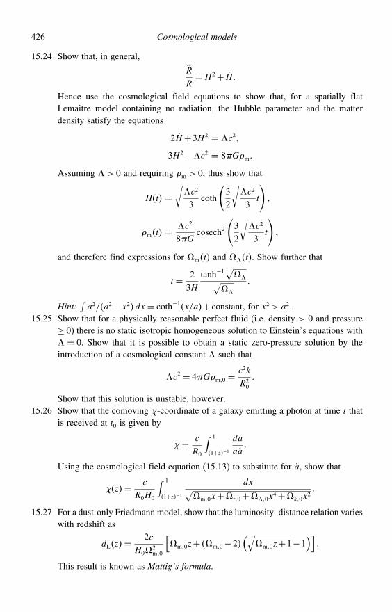
426 Cosmological models
15.24 Show that, in general,
R
R=H2+ H
Hence use the cosmological field equations to show that, for a spatially flatLemaitre model containing no radiation, the Hubble parameter and the matterdensity satisfy the equations
2H+3H2 = $c2
3H2−$c2 = 8Gm
Assuming $> 0 and requiring m > 0, thus show that
Ht =√$c2
3coth
(32
√$c2
3t
)
mt =$c2
8Gcosech2
(32
√$c2
3t
)
and therefore find expressions for mt and $t. Show further that
t = 23H
tanh−1√$√
$
Hint:∫a2/a2−x2dx = coth−1x/a+ constant, for x2 > a2.
15.25 Show that for a physically reasonable perfect fluid (i.e. density > 0 and pressure≥ 0) there is no static isotropic homogeneous solution to Einstein’s equations with$ = 0. Show that it is possible to obtain a static zero-pressure solution by theintroduction of a cosmological constant $ such that
$c2 = 4Gm0 =c2k
R20
Show that this solution is unstable, however.15.26 Show that the comoving -coordinate of a galaxy emitting a photon at time t that
is received at t0 is given by
= c
R0
∫ 1
1+z−1da
aa
Using the cosmological field equation (15.13) to substitute for a, show that
z= c
R0H0
∫ 1
1+z−1dx√
m0x+r0+$0x4+k0x
2
15.27 For a dust-only Friedmann model, show that the luminosity–distance relation varieswith redshift as
dLz=2c
H02m0
[m0z+ m0−2
(√m0z+1−1
)]
This result is known as Mattig’s formula.
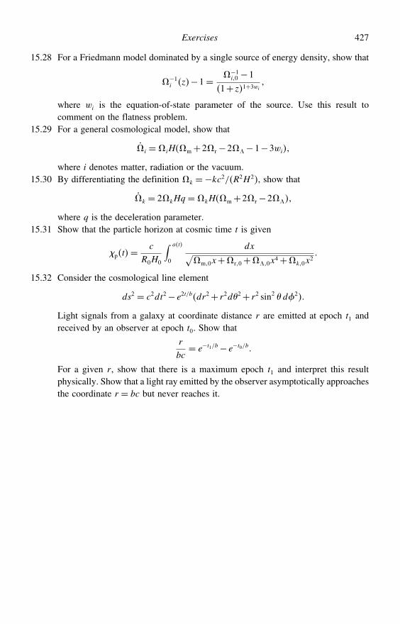
Exercises 427
15.28 For a Friedmann model dominated by a single source of energy density, show that
−1i z−1= −1
i0 −1
1+ z1+3wi
where wi is the equation-of-state parameter of the source. Use this result tocomment on the flatness problem.
15.29 For a general cosmological model, show that
i =iHm+2r−2$−1−3wi
where i denotes matter, radiation or the vacuum.15.30 By differentiating the definition k =−kc2/R2H2, show that
k = 2kHq =kHm+2r−2$
where q is the deceleration parameter.15.31 Show that the particle horizon at cosmic time t is given
pt=c
R0H0
∫ at
0
dx√m0x+r0+$0x
4+k0x2
15.32 Consider the cosmological line element
ds2 = c2dt2− e2t/bdr2+ r2d2+ r2 sin2 d2
Light signals from a galaxy at coordinate distance r are emitted at epoch t1 andreceived by an observer at epoch t0. Show that
r
bc= e−t1/b− e−t0/b
For a given r, show that there is a maximum epoch t1 and interpret this resultphysically. Show that a light ray emitted by the observer asymptotically approachesthe coordinate r = bc but never reaches it.
16
Inflationary cosmology
In the last two sections of the previous chapter, we saw that standard cosmologicalmodels suffer, in particular, from the flatness problem and the horizon problem.To these problems, one might also add the ‘expansion problem’, which askssimply why the universe is expanding at all. Although this appears as an initialcondition in cosmological models, one would hope to explain this phenomenonwith an underlying physical mechanism. In this chapter, we therefore augmentour discussion of cosmological models with a brief outline of the inflationaryscenario, which seeks to solve these problems (and others) and has, over thepast two decades, become a fundamental part of modern cosmological theory.1 Inparticular, we will discuss the effect of inflation on the evolution of the universeas a whole and also consider how inflation gives rise to perturbations in theearly universe that subsequently collapse under gravity to form all the structurewe observe in the universe today. Given the general algebraic complexity ofthese topics (particularly the perturbation analysis), we will adopt the conventionthroughout this chapter that
8G= c = 1
This choice of units makes many of the equations far less cluttered and amountsonly to a rescaling of the scalar field and its potential (see below), which we canremove at the end if desired.
16.1 Definition of inflation
As noted in Section 15.12, the horizon problem is a direct consequence of thedeceleration in the expansion of the universe. Thus, a possible solution is to
1 For a detailed discussion of inflationary cosmology, see, for example, A. Liddle & D. Lyth, CosmologicalInflation and Large-scale Structure, Cambridge University Press, 2000.
428
16.1 Definition of inflation 429
postulate an accelerating phase of expansion, prior to any decelerating phase. Inan accelerating phase, causal contact is better at earlier times and so remotelyseparated parts of our present universe could have ‘coordinated’ their physicalcharacteristics in the early universe. Such an accelerating phase is called a periodof inflation. Hence the basic definition of inflation is that
R > 0 (16.1)
In fact, we may recast this condition in an alternative manner that is physicallymore meaningful by considering the comoving Hubble distance defined in (15.51),namely Ht=H−1t/Rt. The derivative with respect to t is given by
d
dt
(H−1
R
)= d
dt
(1
R
)=− R
R2
and so the condition (16.1) can be written as
d
dt
(H−1
R
)< 0
Thus, an equivalent condition for inflation is that the comoving Hubble distancedecreases with cosmic time. Hence, when viewed in comoving coordinates, thecharacteristic length scale of the universe becomes smaller as inflation proceeds.Let us suppose that, at some period in the early universe, the energy density
is dominated by some form of matter with density and pressure p. The firstcosmological field equation (14.36) (with $= 0 and 8G= c = 1) then reads
R=− 16+3pR (16.2)
Thus, we see that in order for the universe to accelerate, i.e. for inflation to occur,we require that
p <− 13 (16.3)
In other words, we need the ‘matter’ to have an equation of state with negativepressure. In fact, the above criterion can also solve the flatness problem. Thesecond cosmological field equation (with $= 0 and 8G= c = 1) reads
R2 = 13R
2−k (16.4)
430 Inflationary cosmology
During a period of acceleration R > 0, the scale factor must increase faster thanRt ∝ t. Provided that p < −1
3, the quantity R2 will increase during such aperiod as the universe expands and can make the curvature term on the right-hand side negligible, provided that the accelerating phase persists for sufficientlylong.
We could, of course, have included the cosmological-constant terms in thetwo field equations, which would then be equivalent to those for a fluid withan equation of state = −p and so would clearly satisfy the criterion (16.3).However, we have chosen to omit such terms since, as we will see, if ‘matter’in the form of a scalar field exists in the early universe then this can act as aneffective cosmological constant. In order to show that the existence of such fieldsis likely, we must consider briefly the topic of phase transitions in the very earlyuniverse.
16.2 Scalar fields and phase transitions in the very early universe
The basic physical mechanism for producing a period of inflation in the veryearly universe relies on the existence, at such epochs, of matter in a form that canbe described classically in terms of a scalar field (as opposed to a vector, tensoror spinor field, examples of which are provided by the electromagnetic field, thegravitational field and normal baryonic matter respectively). Upon quantisation,a scalar field describes a collection of spinless particles.
It may at first seem rather arbitrary to postulate the presence of such scalarfields in the very early universe. Nevertheless, their existence is suggested by ourbest theories for the fundamental interactions in Nature, which predict that theuniverse experienced a succession of phase transitions in its early stages as itexpanded and cooled. For the purposes of illustration, let us model this expansionby assuming that the universe followed a standard radiation-dominated Friedmannmodel in its early stages, in which case
Rt∝ t1/2 ∝ 1Tt
(16.5)
where the ‘temperature’ T is related to the typical particle energy by T ∼ E/kB.The basic scenario is as follows.
• EP ∼ 1019 GeV> E> EGUT ∼ 1015 GeV The earliest point at which the universe canbe modelled (even approximately) as a classical system is the Planck era, correspondingto particle energies EP ∼ 1019 GeV (or temperature TP ∼ 1032 K) and time scales tP ∼10−43 s (prior to this epoch, it is considered that the universe can be described onlyin terms of some, as yet unknown, quantum theory of gravity). At these extremely
16.3 A scalar field as a cosmological fluid 431
high energies, grand unified theories (GUTs) predict that the electroweak and strongforces are in fact unified into a single force and that these interactions bring theparticles present into thermal equilibrium. Once the universe has cooled to EGUT ∼1014 GeV (corresponding to TGUT ∼ 1027 K), there is a spontaneous breaking of thelarger symmetry group characterising the GUT into a product of smaller symmetrygroups, and the electroweak and strong forces separate. From (16.5), this GUT phasetransition occurs at tGUT ∼ 10−36 s.
• EGUT ∼ 1015 GeV > E > EEW ∼ 100GeV During this period (which is extremelylong in logarithmic terms), the electroweak and strong forces are separate and theseinteractions sustain thermal equilibrium. This continues until the universe has cooledto EEW ∼ 100GeV (corresponding to TGUT ∼ 1015 K), when the unified electroweaktheory predicts that a second phase transition should occur in which the electromagneticand weak forces separate. From (16.5), this electroweak phase transition occurs attEW ∼ 10−11 s.
• EEW ∼ 100GeV>E>EQH ∼ 100MeV During this period the electromagnetic, weakand strong forces are separate, as they are today. It is worth noting, however, thatwhen the universe has cooled to EQH ∼ 100MeV (corresponding to TQH ∼ 1012 K)there is a final phase transition, according to the theory of quantum chromody-namics, in which the strong force increases in strength and leads to the confine-ment of quarks into hadrons. From (16.5), this quark–hadron phase transition occursat tQH ∼ 10−5 s.
In general, phase transitions occur via a process called spontaneous symmetrybreaking, which can be characterised by the acquisition of certain non-zero valuesby scalar parameters known as Higgs fields. The symmetry is manifest whenthe Higgs fields have the value zero; it is spontaneously broken whenever atleast one of the Higgs fields becomes non-zero. Thus, the occurrence of phasetransitions in the very early universe suggests the existence of scalar fields andhence provides the motivation for considering their effect on the expansion of theuniverse. In the context of inflation, we will confine our attention to scalar fieldspresent at, or before, the GUT phase transition (the most speculative of these phasetransitions).
16.3 A scalar field as a cosmological fluid
For simplicity, let us consider a single scalar field present in the very earlyuniverse. The field is traditionally called the ‘inflaton’ field for reasons that willbecome apparent shortly. The Lagrangian for a scalar field (see Section 19.6)has the usual form of a kinetic term minus a potential term:
L= 12g
−V
432 Inflationary cosmology
The corresponding field equation for is obtained from the Euler–Lagrangeequations and reads
2+ dV
d= 0 (16.6)
where 2 ≡ = g is the covariant d’Alembertian operator. A simpleexample is a free relativistic scalar field of mass m, for which the potential wouldbe V = 1
2m22 and the field equation becomes the covariant Klein–Gordon
equation,
2+m2= 0
For the moment, however, it is best to keep the potential function V general.The energy–momentum tensor T for a scalar field can be derived from
this variational approach (see Section 19.12), but in fact we can use our earlierexperience to anticipate its form. By analogy with the forms of the energy–momentum tensor for dust and for electromagnetic radiation, we require that Tis (i) symmetric and (ii) quadratic in the derivatives of the dynamical variable ,and (iii) that T
= 0 by virtue of the field equation (16.6). It is straightforwardto show that the required form must be
T = −g[ 12#
#−V] (16.7)
The energy–momentum tensor for a perfect fluid is
T = +puu−pg
and by comparing the two forms in a Cartesian inertial coordinate system g = in which the fluid is at rest, we see that the scalar field acts like a perfectfluid, with an energy density and pressure given by
= 12
2+V+ 122
p = 12
2−V− 162
(16.8)
In particular, we note that if the field were both temporally and spatiallyconstant, its equation of state would be p =− and so the scalar field wouldact as a cosmological constant with $= V (with 8G= c= 1). In general thisis not the case, but we will assume that the spatial derivatives can be neglected.This is equivalent to assuming that is a function only of t and so has no spatialvariation.
16.4 An inflationary epoch 433
16.4 An inflationary epoch
Let us suppose that the scalar field does not interact (except gravitationally) withany other matter or radiation that may be present. In this case, the scalar fieldwill independently obey an equation of motion of the form (14.39), namely
+3+pR
R= 0
Substituting the expressions (16.8) and assuming no spatial variations, we quicklyfind that the equation of motion of the scalar field is
+3H+ dV
d= 0 (16.9)
The form of this equation will be familiar to any student of classical mechanicsand allows one to develop an intuitive picture of the evolution of the scalar field.If one thinks of the plot of the potential V versus as defining some curve, thenthe motion of the scalar field value is identical to that of a ball rolling (or,more precisely, sliding) under gravity along the curve, subject to a frictional forceproportional to its speed (and to the value of the Hubble parameter).
Let us assume further that there is some period when the scalar field dominatesthe energy density of the universe. Moreover we will demand that the scalar fieldenergy density is sufficient large that we may neglect the curvature term in thecosmological field equation (16.4) although this is not strictly necessary.2 Thus,we may write (16.4) as
H2 = 13
[12
2+V]. (16.10)
This equation and (16.9) thus provide a set of coupled differential equations in and H that determine completely the evolution of the scalar field and thescale factor of the universe during the epoch of scalar-field domination. From ourcriterion (16.3) and the expressions (16.8), we see that inflation will occur (i.e.R > 0) provided that
2 < V (16.11)
2 Note that, even if the curvature term is not negligible to begin with, the initial stages of inflation will soonrender it so.
434 Inflationary cosmology
16.5 The slow-roll approximation
The inflation equations (16.9) and (16.10) can easily be solved numerically, andeven analytically for some special choices of V. In general, however, ananalytical solution is only possible in the slow-roll approximation, in which it isassumed that 2 V. On differentiating, this in turn implies that dV/d
and so the -term can be neglected in the equation of motion (16.9), to yield
3H=−dV
d (16.12)
Moreover, the cosmological field equation (16.10) becomes simply
H2 = 13V (16.13)
It is worth noting that, in this approximation, the rate of change of the Hubbleparameter and the scalar field can be related very easily. Differentiating (16.13)with respect to t and combining the result with (16.12), one obtains
H =− 12
2 (16.14)
The conditions for inflation in the slow-roll approximation can be put intoa useful dimensionless form. Using the two equations above and the condition2 V, it is easy to show that
≡ 12
(V ′
V
)2
1 (16.15)
where V ′ ≡ dV/d and the factor 12 is included according to the standard conven-
tion. Differentiating the above expression with respect to , one also finds that
≡ V ′′
V 1 (16.16)
These two conditions make good physical sense in that they require the potentialV to be sufficiently ‘flat’ that the field ‘rolls’ slowly enough for inflation tooccur. It is worth noting, however, that these conditions alone are necessary butnot sufficient conditions for inflation, since they limit only the form of V andnot that of , which could be chosen to violate the condition (16.11). Thus, onemust also assume that (16.11) holds.
It is worth considering the special case in which the potential V is sufficientlyflat that, during (some part of) the period of inflation, its value remains roughly
16.7 The amount of inflation 435
constant. From (16.12), we see that in this case the Hubble parameter is constantand the scale factor grows exponentially:
Rt∝ exp(√
13Vt
)
16.6 Ending inflation
As the field value ‘rolls’ down the potential V, the condition (16.11) willeventually no longer hold and inflation will cease. Equivalently, in the slow-roll approximation, the conditions (16.15, 16.16) will eventually no longer besatisfied. If the potential V possesses a local minimum, which is usually thecase in most inflationary models, the field will no longer roll slowly downhill butwill oscillate about the minimum of the potential, the oscillation being graduallydamped by the 3H friction term in the equation of motion (16.9). Eventually,the scalar field is left stationary at the bottom of the potential. If the value ofthe potential at its minimum is Vmin > 0 then clearly the condition (16.11) isagain satisfied and the universe continues to inflate indefinitely. Moreover, in thiscase p =− and so the scalar field acts as an effective cosmological constant$ = Vmin. If Vmin = 0, however, no further inflation occurs, the scalar field haszero energy density and the dynamics of the universe is dominated by any otherfields present.
In fact, the scenario outlined above would occur only if the scalar field werenot coupled to any other fields, which is almost certainly not the case. In practice,such couplings will cause the scalar field to decay during the oscillatory phaseinto pairs of elementary particles, into which the energy of the scalar field is thusconverted. The universe will therefore contain roughly the same energy densityas it did at the start of inflation. The process of decay of the scalar field intoother particles is therefore termed reheating. These particles will interact witheach other and subsequently decay themselves, leaving the universe filled withnormal matter and radiation in thermal equilibrium and thereby providing theinitial conditions for a standard cosmological model.
16.7 The amount of inflation
Although the motivation for the introduction of the inflationary scenario was (inpart) to solve the flatness and horizon problems, we have not yet considered theamount of inflation required to achieve this goal. From our present understanding
436 Inflationary cosmology
of particle physics, it is thought that inflation occurs at around the era of the GUTphase transition, or earlier. For illustration, let us assume that the universe hasfollowed a standard radiation-dominated Friedmann model for (the majority of)its history since the epoch of inflation at t ∼ t∗. From (16.5), we thus have
R∗R0∼(t∗t0
)1/2
∼ T0T∗
(16.17)
where T0 ∼ 3K is the present-day temperature of the cosmic microwave back-ground radiation and t0 ∼ 1/H0 ∼ 1018 s is the present age of the universe.Let us first consider the flatness problem. From (15.47), the ratio of the spatial
curvature density at the inflationary epoch to that at the present epoch is given by
k∗k0
=(H0
H∗
)2(R0
R∗
)2
∼ t∗t0 (16.18)
where we have used the fact that H0/H∗ ∼ t∗/t0. Assuming inflation to occurat some time between the Planck era and the GUT phase transition, so thattP < t∗ < tGUT, from Section 16.2 we find that the ratio (16.18) lies in the range∼ 10−60–10−54. Thus, if the present-day value k0 is of order unity then therequired degree of fine-tuning of k∗ is extreme, in a standard cosmologicalmodel. Since the ratio above depends on 1/R2∗ we thus find that, to solve theflatness problem (in order that k∗ can also be of order unity), we require thescale factor to grow during inflation by a factor ∼ 1027–1030. In terms of therequired number N of e-foldings of the scale factor, we thus have
N 60–70 (flatness problem)
We now turn to the horizon problem. If the universe followed a standardradiation-dominated Friedmann model in its earliest stages, then (reinstating c forthe moment) the particle horizon at the inflationary epoch is
dp∗ = 2ct∗
which, taking tP < t∗ < tGUT, gives the size of a causally connected region at thistime as ∼ 10−33–10−27 m. From (16.17), we see that the size of such a regiontoday would be only ∼ 10−3–1m. The current size of the observable universe,however, is given approximately by the present-day Hubble distance,
dH0 = cH−10 ∼ 1026 m ∼ 3000Mpc
16.8 Starting inflation 437
To solve the horizon problem, we thus require the scale factor to grow by a factorof ∼ 1026–1029 during the period of inflation. Expressing this result in terms ofthe required number N of e-foldings, we once again find
N 60–70 (horizon problem)
We have thus found that both the flatness and the horizon problems can besolved by a period of inflation, provided that the scale factor undergoes more thanaround 60–70 e-foldings during this period. We may now consider the constraintsplaced by this condition on the form of the scalar field potential V. In theslow-roll approximation, the number of e-foldings that occur while the scalar field‘rolls’ from 1 to 2 is given by
N =∫ t2
t1
H dt =∫ 2
1
H
d=−
∫ 2
1
V
V ′d
If the potential is reasonably smooth then V ′ ∼ V/. Thus, if = start−endis the range of -values over which inflation occurs, one finds N ∼ 2. Inorder to solve the flatness and horizon problems, one hence requires 1.
16.8 Starting inflation
The observant reader will have noticed that so far we have not discussed howinflation may start. During the inflationary epoch, the scalar field rolls downhillfrom start to end, but we have not yet considered how the universe can arrive atan appropriate starting state. The details will depend, in fact, on the precise infla-tionary cosmology under consideration, but there are generally two main classesof model. In early models of inflation, the inflationary epoch is an ‘interlude’ inthe evolution of a standard cosmological model. In such models, the inflaton field is usually identified with a scalar Higgs field operating during the GUT phasetransition. It is thus assumed that the universe was in a state of thermal equi-librium from the very beginning and that this state was relatively homogeneousand large enough to survive until the beginning of inflation at the GUT era; anexample of this sort is provided by the ‘new’ inflation model discussed below inSection 16.9. In more recent models of inflation, the scalar field is not identifiedwith the Higgs field in the GUT phase transition but is some generic scalar fieldpresent in the very early universe. In particular, in these models the universe mayinflate soon after it exits the Planck era, thereby avoiding the above assumptionsregarding the state of the universe prior to the inflationary epoch; an example ofsuch a model is the chaotic inflation scenario discussed in Section 16.10. We will
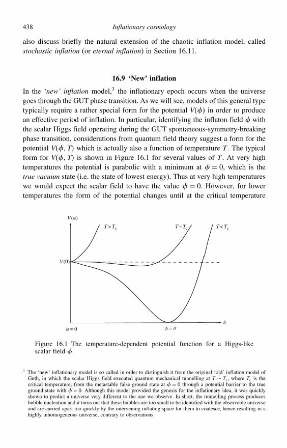
438 Inflationary cosmology
also discuss briefly the natural extension of the chaotic inflation model, calledstochastic inflation (or eternal inflation) in Section 16.11.
16.9 ‘New’ inflation
In the ‘new’ inflation model,3 the inflationary epoch occurs when the universegoes through the GUT phase transition. As we will see, models of this general typetypically require a rather special form for the potential V in order to producean effective period of inflation. In particular, identifying the inflaton field withthe scalar Higgs field operating during the GUT spontaneous-symmetry-breakingphase transition, considerations from quantum field theory suggest a form for thepotential VT which is actually also a function of temperature T . The typicalform for VT is shown in Figure 16.1 for several values of T . At very hightemperatures the potential is parabolic with a minimum at = 0, which is thetrue vacuum state (i.e. the state of lowest energy). Thus at very high temperatureswe would expect the scalar field to have the value = 0. However, for lowertemperatures the form of the potential changes until at the critical temperature
V(0)
V(φ)
φ = 0φ
φ = σ
T > Tc T ~ Tc T < Tc
Figure 16.1 The temperature-dependent potential function for a Higgs-likescalar field .
3 The ‘new’ inflationary model is so called in order to distinguish it from the original ‘old’ inflation model ofGuth, in which the scalar Higgs field executed quantum mechanical tunnelling at T ∼ Tc, where Tc is thecritical temperature, from the metastable false ground state at = 0 through a potential barrier to the trueground state with > 0. Although this model provided the genesis for the inflationary idea, it was quicklyshown to predict a universe very different to the one we observe. In short, the tunnelling process producesbubble nucleation and it turns out that these bubbles are too small to be identified with the observable universeand are carried apart too quickly by the intervening inflating space for them to coalesce, hence resulting in ahighly inhomogeneous universe, contrary to observations.
16.9 ‘New’ inflation 439
T = Tc the potential develops a lower energy state than that at = 0. Thus thisnew non-zero value of is now the true vacuum state, and = 0 is now a falsevacuum state. For even lower values the new true vacuum state becomes morepronounced until a final form is reached for ‘low’ temperatures.
Let us now consider the evolution of the scale factor Rt, the radiation energydensity r and the scalar field .
Phase 1 When the temperature is very high, i.e. far above the GUT phasetransition scale of Tc ∼ 1027 K, from Figure 16.1 we would expect the scalar fieldto have the value = 0 (i.e. at the true vacuum state for these temperatures),and Figure 16.1 shows that it will remain at = 0. Since r ∝ R−4, however, wewould expect the radiation to dominate over the scalar field at very early epochs.Thus we have the standard early-time radiation-dominated Friedmann model, inwhich we can neglect the curvature constant k. Thus, for T Tc,
R∝ t1/2 r ∝ t−2 = 0
Phase 2 It is clear from the above equations that there will come a time whenthe scalar-field energy density dominates over that of the radiation. Provided thatthis occurs for T> Tc the scalar field remains at = 0, in which case it acts as aneffective cosmological constant of value $= V0. Thus, in this phase, the scalefactor undergoes an exponential expansion:
Rt∝ exp
(√13V0t
)
As a result of the exponential expansion, however, there is a correspondingexponential decrease in the temperature T , which results in a rapid change ofthe potential function. Thus T ∼ Tc is reached very quickly, and so this phaseis extremely short-lived, and very little expansion is actually achieved. Indeed, ifT ∼ Tc is reached before the scalar-field energy density dominates over that ofthe radiation then phase 2 does not occur at all.
Phase 3 Once T ∼ Tc, we see from Figure 16.1 that the scalar field is now able toroll downhill away from = 0 and so the GUT phase transition occurs. Providedthat the potential is sufficiently flat, the slow-roll approximation holds and theuniverse inflates, the evolution of the scalar field being determined by (16.12)and the Hubble parameter by (16.13). If the potential is roughly constant thenthe exponential expansion continues. The rapid growth of the scale factor onceagain causes the evolution of the potential function as the temperature drops. The
440 Inflationary cosmology
duration of this period of inflation depends critically on the flatness and lengthof the plateau of the V function for T < Tc. For certain ‘reasonable’ potentialsthe universe can easily inflate in such a way that the number of e-foldingsN 60, and can be considerably larger. This is therefore the main inflationaryphase. According to detailed calculations, phase 3 occurs between t1 ∼ 10−36 sand t2 ∼ 10−34 s and the scale factor increases by a factor of around 1050.
Phase 4 Eventually, the slow-roll approximation fails and inflation ends. Thescalar field then rolls rapidly down towards the true vacuum state at = # ,oscillating about the minimum point, and follows the behaviour outlined inSection 16.6. In particular, if V#= 0 then the universe will revert to the standardradiation-dominated Friedmann model with
Rt∝ t1/2
Hence, at t ∼ 10−34 s, the universe starts a standard Friedmann expansion, albeitwith the desired ‘initial’ conditions. Thus, the inflationary model incorporates allthe observationally verified predictions of the standard cosmological models.
Although the ‘new’ inflation model still has its advocates, it suffers fromundesirable features. In particular, the scenario only provides an effective periodof inflation if VT has a very flat plateau near = 0, which is somewhatartificial. Moreover, the period of thermal equilibrium prior to the inflationaryphase (so one can speak sensibly of the universe having a particular temperature)requires many particles to interact with one another, and so already one requiresthe universe to be very large and contain many particles. Finally, the universecould easily recollapse before inflation starts. As a result of these difficulties, newinflation may not be a viable model, and so there are strong theoretical reasonsto believe that the inflaton field cannot be identified with the GUT symmetry-breaking Higgs field. Thus, the hope that GUTs could provide the mechanism forthe homogeneity and flatness of the universe may have to be abandoned.
16.10 Chaotic inflation
In more recent models of inflation, the scalar field is not identified withthe Higgs field in the GUT phase transition but is regarded as a generic scalarfield present in the very early universe. In particular, these models invoke theidea of chaotic inflation. In this scenario, as the universe exits the Planck eraat t ∼ 10−43 s the initial value of the scalar field start is set chaotically, i.e. itacquires different random values in different regions of the universe. In someregions, start is somewhat displaced from the minimum of the potential and
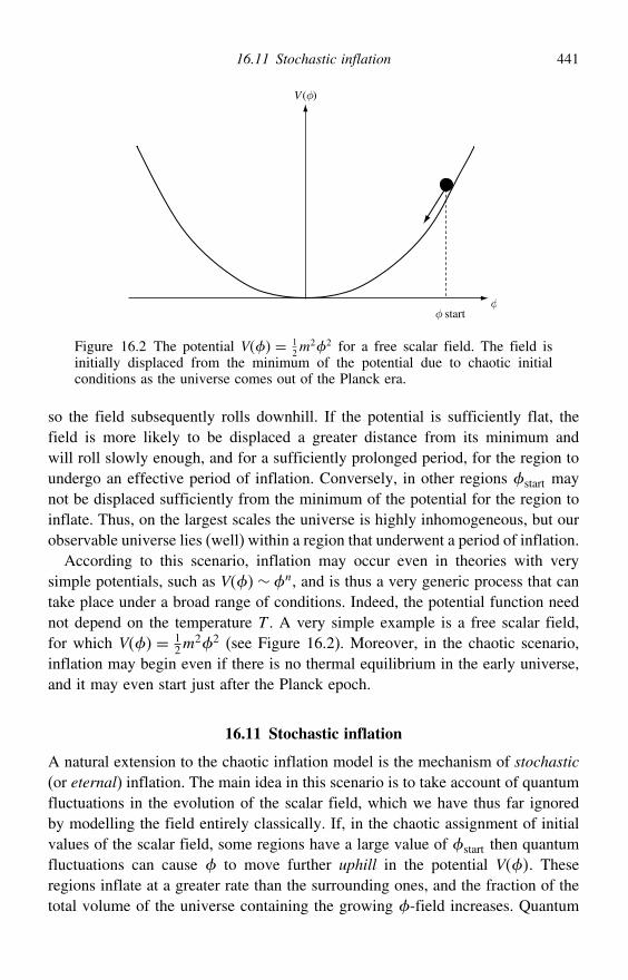
16.11 Stochastic inflation 441
φ
V(φ)
φ start
Figure 16.2 The potential V = 12m
22 for a free scalar field. The field isinitially displaced from the minimum of the potential due to chaotic initialconditions as the universe comes out of the Planck era.
so the field subsequently rolls downhill. If the potential is sufficiently flat, thefield is more likely to be displaced a greater distance from its minimum andwill roll slowly enough, and for a sufficiently prolonged period, for the region toundergo an effective period of inflation. Conversely, in other regions start maynot be displaced sufficiently from the minimum of the potential for the region toinflate. Thus, on the largest scales the universe is highly inhomogeneous, but ourobservable universe lies (well) within a region that underwent a period of inflation.
According to this scenario, inflation may occur even in theories with verysimple potentials, such as V∼ n, and is thus a very generic process that cantake place under a broad range of conditions. Indeed, the potential function neednot depend on the temperature T . A very simple example is a free scalar field,for which V = 1
2m22 (see Figure 16.2). Moreover, in the chaotic scenario,
inflation may begin even if there is no thermal equilibrium in the early universe,and it may even start just after the Planck epoch.
16.11 Stochastic inflation
A natural extension to the chaotic inflation model is the mechanism of stochastic(or eternal) inflation. The main idea in this scenario is to take account of quantumfluctuations in the evolution of the scalar field, which we have thus far ignoredby modelling the field entirely classically. If, in the chaotic assignment of initialvalues of the scalar field, some regions have a large value of start then quantumfluctuations can cause to move further uphill in the potential V. Theseregions inflate at a greater rate than the surrounding ones, and the fraction of thetotal volume of the universe containing the growing -field increases. Quantum
442 Inflationary cosmology
fluctuations within these regions lead in turn to the production of some newinflationary regions that expand still faster. This process thus leads to eternalself-reproduction of the inflationary universe.
16.12 Perturbations from inflation
We have seen that inflation can solve the horizon and flatness problems. Arguablyits greatest success so far, however, is to provide a mechanism by which thefluctuations needed to seed the development of structure within the universe canbe generated. This topic is the subject of much current research, and we can giveonly a limited treatment here. Nevertheless, by following through the equations forstructure generation and development in the simplest case, namely for a spatiallyflat universe with a simple ‘gauge choice’ (see below), we hope that the readerwill be able to get a flavour of the physics involved.
The current opinion of how structure in the universe originated is that it was viaamplification, during a period of inflation, of initial quantum irregularities of thescalar field that drives inflation. Thus what we need to do can be divided into twobroad categories. First, we need to work out the equations of motion for spatialperturbations in the scalar field. This can be done classically, i.e. taking the scalarfield as a classical source linked self-consistently to the gravitational field via aclassical energy–momentum tensor. Second, we need to derive initial conditionsfor these perturbations, and this demands that we understand the quantum fieldtheory of the perturbations themselves. This sounds formidable but actually turnsout to be no more complicated than considering the quantum physics of a masson a spring, albeit one in which the mass changes as a function of time. Thesetopics are discussed in detail in the remainder of this chapter.
16.13 Classical evolution of scalar-field perturbations
We assume that the scalar field , which hitherto has been a function of cosmictime t only, now has perturbations that are functions of space and time. We canthus write
t→ 0t+t x (16.19)
These perturbations will lead to a perturbed energy–momentum tensor, which weshall derive shortly. The Einstein field equations then imply that the Einsteintensor is also perturbed away from its background value. In turn, therefore, wemust have a metric different from the Friedmann–Robertson–Walker one assumedso far. We thus need to assume a form for this metric in order to calculate thenew Einstein tensor. It is at this point we must make the choice of ‘gauge’ (i.e.
16.13 Classical evolution of scalar-field perturbations 443
coordinate system) referred to above. Once perturbations are present there is nopreferred way to define a spacetime slicing of the universe. The details of this arequite subtle but amount simply to the fact that by choosing different coordinatesystems we can change the apparent character of the perturbations considerably.For example, suppose that we choose, as a new time coordinate, one for whichsurfaces of constant time have a constant value of the new perturbed scalar fieldon them. This is always possible and, in such a gauge, the spatial fluctuations of have apparently totally vanished!
To meet such problems, methods that deal only with gauge-invariant quantitieshave been developed. We will make contact with such methods below, whenwe introduce the so-called ‘curvature’ perturbations. These are gauge invariantand therefore represent physical quantities. To reach this point, however, we firstwork with a specific simple form of gauge known as the as the longitudinalor Newtonian gauge, and indeed with a restricted form of this – one whereonly one extra function (known here as a ‘potential function’) is introduced.The justification for using such a restricted form is that it leads to an Einsteintensor with the correct extra degrees of freedom to match the extra terms in thescalar-field energy–momentum tensor arising from the field perturbations.
For a spatially flat (k = 0) background FRW model, which is what we willassume, we adopt Cartesian comoving coordinates and write the perturbed metric as
ds2 = 1+2% dt2− 1−2%R2t(dx2+dy2+dz2
) (16.20)
where % is a general infinitesimal function of all four coordinates (and shouldnot to be confused with the scalar field ). Its assumed smallness means that wewill only need to consider quantities to first order in %. A general discussion ofthis linearising process is presented in the next chapter, but for the time being wesimply note that one can consider % as representing the Newtonian potential ofthe perturbations. For instance, for a spherically symmetric perturbation of massM and radius r , if we put %=GM/rc2 then the first term of (16.20) recovers thett-term of the Schwarzschild metric.
The perturbed Einstein field equations
We now need to find both the new energy–momentum tensor of the scalar field and the new Einstein tensor corresponding to our perturbed metric. Equatingthem will link our two perturbation variables and % and provide us with theequations of evolution that we need. The first step is to calculate the connectioncoefficients corresponding to the perturbed metric (16.20) to first order in %.These are easily shown to take the form #
= 0#+ #
, where the first
444 Inflationary cosmology
term corresponds to the connection coefficients of the unperturbed metric (i.e.with % = 0) and the perturbation terms are given by
00 = %
0ii = −R2%+4H%
i00 =
1R2
i%
ii = −%
In these expressions, H = R/R is the Hubble parameter of the unperturbed back-ground, and no sum over repeated i indices is implied. The remaining perturbedconnection coefficients either follow from symmetry or are zero.
These connection coefficients yield a Riemann and hence an Einstein tensor.Again working to first order in %, the perturbed part of the Einstein tensor isfound to be
G0i =−2i%+H%
G00 =−22%−3H%−3H2%
Gii = 2 %+4%H+ 2H+3H2%
(16.21)
where again no sum over repeated i indices is implied and the remaining entrieseither follow from symmetry or are zero. The symbol 2 here denotes the spatialLaplacian, which in this simple flat case is given by
2 = 1R2
(2
x2+ 2
y2+ 2
z2
) (16.22)
It is worth noting that, in the entries of (16.21), the time derivative of the Hubbleparameter appears. From (16.14), this can be rewritten as
H =− 12
20 (16.23)
remembering that this equation now applies to the background FRW spacetime.We also need to evaluate the perturbed part of the scalar-field energy–
momentum tensor. Substituting (16.19) into (16.7) and working to first order in, one quickly finds that
T 0i = 0i
T 00 =−2
0%+ 0+V ′
T ii = 2
0%− 0+V ′
(16.24)
16.13 Classical evolution of scalar-field perturbations 445
where V ′ = dV/d0 and the remaining components either follow from symmetryor are zero.
We may now use the Einstein field equations to relate the Einstein tensor andthe scalar-field energy–momentum tensor. Since the unperturbed part of the fieldequations is automatically satisfied, one simply requires that G
=−T (since
& = 8G/c4 equals unity in our chosen system of units). We may thus equate,with the inclusion of a minus sign, the components shown in equations (16.21)and (16.24). At first sight, it is by no means obvious that we have allowedourselves enough freedom in including only one extra function, %, in the metric.Nevertheless, as we now show, everything in fact works out. Let us start with the(0i
)-components, for which we have the equation
2i%+H%= 0i (16.25)
Remembering that H and 0 have no spatial dependence, we can integrate thisimmediately to obtain
%+H% = 12 0 (16.26)
One next equates the(ii
)-components, which gives
−2 %+4%H+ 2H+3H2%= 20%− 0+V ′ (16.27)
but we may show that this contains no information beyond that already obtainedfrom the
(0i
)-components. In particular, differentiating (16.26) with respect to time
gives
%+ H%+H% = 12 0+ 1
2 0 (16.28)
then, using equations (16.9) and (16.23) to substitute for 0 and H respectively,one finds that (16.27) is satisfied if (16.26) holds, thus establishing consistency.The only new information must therefore come from equating the
(00
)-components.
Using (16.28) and eliminating V ′ again then yields
(20+22
)% = 2
0d
dt
(
0
) (16.29)
Perturbation equations in Fourier space
The results (16.26) and (16.29) are the basic equations relating % and . Tomake further progress, however, it is convenient to work instead in terms ofthe Fourier decomposition of these quantities and analyse what happens to aperturbation corresponding to a given comoving spatial scale. Thus, we assume
446 Inflationary cosmology
that % and are decomposed into a superposition of plane-wave states withcomoving wavevector k, so that
%x= 123/2
∫%k expik · xd3k
where (with a slight abuse of notation) x = x y z and a similar expressionholds for . The evolution of a mode amplitude %k depends only on the
comoving wavenumber k = k; the corresponding actual physical wavenumberis k/Rt. We thus work simply in terms of %k and k. In terms of thesevariables, the action of 2 will be just to multiply %k by −k2/R2t, whereasthe time derivatives remain unchanged. Equations (16.26) and (16.29) thereforebecome
%k+H%k = 12 0k(
1− 2k2
R220
)%k =
d
dt
(k
0
)
(16.30)
Thus, we see that we have obtained two coupled first-order differential equationsfor the quantities %k and k, which are the amplitudes of the plane-waveperturbations of comoving wavenumber k in the metric and in the scalar fieldrespectively. Clearly, what we could do next is to eliminate one quantity in termsof derivatives of the other and then obtain a single second-order equation interms of just one of them (plus the background quantities, of course, but theevolution of these is assumed known). In fact, this leads to rather messy equationsand, moreover, in terms of the discussion given above the results are not gaugeinvariant, since neither %k nor k is gauge invariant on its own.
16.14 Gauge invariance and curvature perturbations
As mentioned above, gauge invariance is related to how we define spatial ‘slices’of the perturbed spacetime. By transforming to a new time coordinate, one canapparently make the perturbations in the scalar field come and go at will. Thereare two ways to take care of this difficulty. First, one can choose variables that areinsensitive to such changes and therefore definitely describe something physical.These are called gauge-invariant variables. Second, one can use variables whichwould change if one altered the slicing but which are defined relative to a particularslicing that can itself be defined physically. These are then also physical variablesand are, perhaps confusingly, also sometimes called gauge invariant, although thisis not really a good description. Note that changing spatial coordinates within a
16.14 Gauge invariance and curvature perturbations 447
particular slicing also induces changes, but these are not relevant to our discussionhere and we concentrate just on changes in time coordinate.
Let us start our discussion by taking the first of the two routes outlined above,namely describing the perturbations in terms of truly gauge-invariant quantities.For any scalar function f in spacetime, consider the effects upon it of the changein time coordinate t→ t′ = t+t. We may define a new, perturbed, function by
f ′t′= ft (16.31)
where, as just stated, we suppress the x-dependences in what follows. Thus, tofirst order in t, we may write
f ′t= f ′t′ −t≈ ft− f t (16.32)
where we do not have to specify whether it is f or f ′ that is being differentiatedwith respect to time to obtain f or whether the latter is evaluated at t or t′, sincethese would be second-order differences. Hence the perturbation in the scalarfunction due to the ‘gauge transformation’ t→ t+t is given by4
f =−ft (16.33)
We may now evaluate the change in the perturbed spacetime metric corre-sponding to the gauge transformation t→ t+t. To do this, however, one mustdistinguish between the two occurrences of the %-variable in (16.20). For anarbitrary scalar perturbation, the general form of the perturbed metric in facttakes the form
ds2 = 1+2*dt2− 1−2%R2t(dx2+dy2+dz2
) (16.34)
in which * and % are different functions. Nevertheless, for matter with no‘anisotropic stress’ (so that all the off-diagonal components of the space partof the stress–energy tensor are zero), the two functions may be taken as equal;this is the case for a perfect fluid or a scalar field and hence leads to (16.20).Even in this case, however, the two functions behave differently under the gaugetransformation. We need consider only the %-function above, which clearly takesthe role of a spatial curvature term since it modifies the space part of the metricby a multiplicative factor. Under t→ t+t we find that
R21−2%→ R21−2%+[2RR1−2%−2R2%
]t (16.35)
4 This is the simplest version of the ‘Lie derivative’, which describes the change in a (possibly tensor) functionwhen ‘dragged back’ along ‘flow lines’ in parameter space; see, for example, B. Schutz, Geometrical Methodsof Mathematical Physics, Cambridge University Press, 1980.
448 Inflationary cosmology
Since both % and t are infinitesimal, we may employ the same arguments thatled to (16.33). Then, to first order, we have
% =Ht (16.36)
where we have also used the fact that RR = R2H . Thus, for any scalar functionf with perturbations f , we see that the combination
f =%+ H f
f(16.37)
is gauge invariant under the gauge transformation t→ t+t that we are consid-ering, since to first order we have
f → ′f =%+Ht+ Hf − ft
f= f (16.38)
Thus, for the specific example of our scalar-field perturbation , we mayidentify the corresponding gauge-invariant quantity as
=%+ H
0
(16.39)
We will therefore use this variable (or its Fourier transform) in our subsequentdiscussion in later sections. In the literature this quantity is called the curvatureperturbation, for reasons that will become clear shortly.
Before going on to consider the evolution of these curvature perturbations,let us first discuss briefly the second route outlined at the start of this sectionfor defining a physically meaningful perturbation variable. This route can beillustrated directly with the %-function, and one begins by defining the quantity
≡ −%co (16.40)
where the subscript indicates that % is to be evaluated on comoving slices. By‘comoving’ we mean a time-slicing that is orthogonal to the worldlines of the‘fluid’ that makes up the matter. For an ordinary fluid, this would amount tochoosing frames in which, at each instant and position, the fluid appears to beat rest. The same applies here and, because the frame involved is physicallydefined, the variable , which measures the spatial curvature in the given frame,is itself physically well defined. Thus the quantity is also called the ‘curvature
16.15 Classical evolution of curvature perturbations 449
perturbation’ in the literature. As we now show, it is in fact equal to minus thevariable defined in (16.39), and so both may be described as such.
For any scalar density perturbation , one can write the spatial curvature inthe comoving slice as
=−+Hco
(16.41)
Let us therefore consider what happens for the particular case of a perturbation ina scalar field. As shown in (16.24), the
(0i
)-components of the perturbed stress–
energy tensor read
T 0i = 0 i (16.42)
In the comoving frame, this momentum density must vanish, by definition, andso the scalar-field perturbation cannot depend on the spatial coordinates and thusvanishes. Hence, for a scalar field, we have
=− (16.43)
16.15 Classical evolution of curvature perturbations
We now consider the evolution of the Fourier transform of the gauge-invariantperturbation (16.39), namely
k ≡%k+Hk
0
(16.44)
which is clearly itself gauge invariant. Using (16.30), the second-order differentialequation satisfied by this quantity is quite simply shown to be
k+(20
H+ 20
0
+3H
)k+
k2
R2k = 0 (16.45)
Given a potential V0 and some initial conditions forH and 0, we can integratethe background evolution equations numerically and obtain H and 0 as functionsof cosmic time t. If we simultaneously integrate k using (16.45), we can therebytrace the evolution of the curvature perturbation over the time period of interest.An example of the results of this procedure is shown in Figures 16.3 and 16.4,
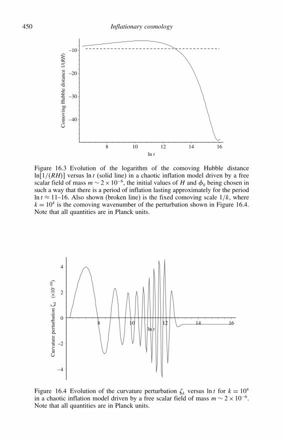
450 Inflationary cosmology
Com
ovin
g H
ubbl
e di
stan
ce 1
/(R
H)
–40
–30
–20
–10
8 10 12 14 16ln t
Figure 16.3 Evolution of the logarithm of the comoving Hubble distanceln 1/RH versus ln t (solid line) in a chaotic inflation model driven by a freescalar field of mass m∼ 2×10⁻⁶, the initial values of H and 0 being chosen insuch a way that there is a period of inflation lasting approximately for the periodln t ≈ 11–16. Also shown (broken line) is the fixed comoving scale 1/k, wherek= 104 is the comoving wavenumber of the perturbation shown in Figure 16.4.Note that all quantities are in Planck units.
–4
–2
0
2
4
8 10 12 14 16ln t
Cur
vatu
re p
ertu
rbat
ion
ζ k
(×10
–10 )
Figure 16.4 Evolution of the curvature perturbation k versus ln t for k = 104
in a chaotic inflation model driven by a free scalar field of mass m∼ 2×10⁻⁶.Note that all quantities are in Planck units.
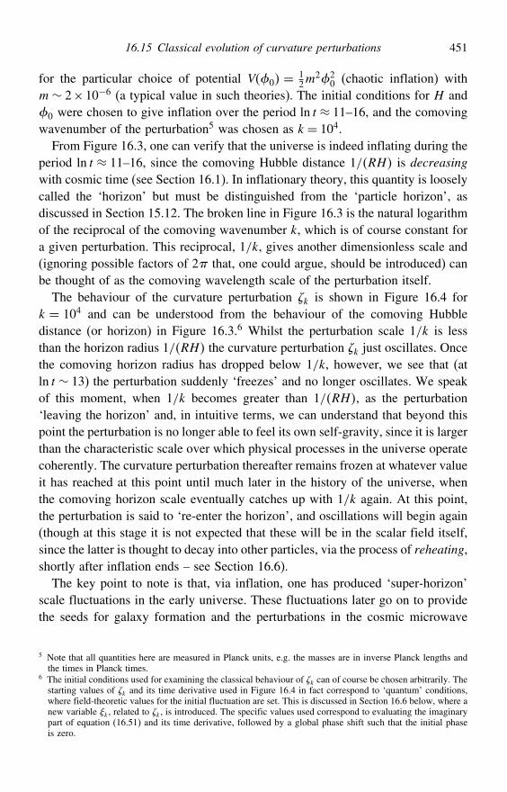
16.15 Classical evolution of curvature perturbations 451
for the particular choice of potential V0 = 12m
220 (chaotic inflation) with
m∼ 2×10⁻⁶ (a typical value in such theories). The initial conditions for H and0 were chosen to give inflation over the period ln t ≈ 11–16, and the comovingwavenumber of the perturbation5 was chosen as k= 104.
From Figure 16.3, one can verify that the universe is indeed inflating during theperiod ln t ≈ 11–16, since the comoving Hubble distance 1/RH is decreasingwith cosmic time (see Section 16.1). In inflationary theory, this quantity is looselycalled the ‘horizon’ but must be distinguished from the ‘particle horizon’, asdiscussed in Section 15.12. The broken line in Figure 16.3 is the natural logarithmof the reciprocal of the comoving wavenumber k, which is of course constant fora given perturbation. This reciprocal, 1/k, gives another dimensionless scale and(ignoring possible factors of 2 that, one could argue, should be introduced) canbe thought of as the comoving wavelength scale of the perturbation itself.
The behaviour of the curvature perturbation k is shown in Figure 16.4 fork = 104 and can be understood from the behaviour of the comoving Hubbledistance (or horizon) in Figure 16.3.6 Whilst the perturbation scale 1/k is lessthan the horizon radius 1/RH the curvature perturbation k just oscillates. Oncethe comoving horizon radius has dropped below 1/k, however, we see that (atln t ∼ 13) the perturbation suddenly ‘freezes’ and no longer oscillates. We speakof this moment, when 1/k becomes greater than 1/RH, as the perturbation‘leaving the horizon’ and, in intuitive terms, we can understand that beyond thispoint the perturbation is no longer able to feel its own self-gravity, since it is largerthan the characteristic scale over which physical processes in the universe operatecoherently. The curvature perturbation thereafter remains frozen at whatever valueit has reached at this point until much later in the history of the universe, whenthe comoving horizon scale eventually catches up with 1/k again. At this point,the perturbation is said to ‘re-enter the horizon’, and oscillations will begin again(though at this stage it is not expected that these will be in the scalar field itself,since the latter is thought to decay into other particles, via the process of reheating,shortly after inflation ends – see Section 16.6).
The key point to note is that, via inflation, one has produced ‘super-horizon’scale fluctuations in the early universe. These fluctuations later go on to providethe seeds for galaxy formation and the perturbations in the cosmic microwave
5 Note that all quantities here are measured in Planck units, e.g. the masses are in inverse Planck lengths andthe times in Planck times.
6 The initial conditions used for examining the classical behaviour of k can of course be chosen arbitrarily. Thestarting values of k and its time derivative used in Figure 16.4 in fact correspond to ‘quantum’ conditions,where field-theoretic values for the initial fluctuation are set. This is discussed in Section 16.6 below, where anew variable k, related to k, is introduced. The specific values used correspond to evaluating the imaginarypart of equation (16.51) and its time derivative, followed by a global phase shift such that the initial phaseis zero.
452 Inflationary cosmology
background radiation that we observe today. By studying the distribution ofgalaxies and CMB fluctuations as a function of scale, it is possible to obtain anidea of the underlying primordial spectrum of perturbations that produced them.Thus, by predicting this primordial spectrum, we can perform a test of the wholeinflationary picture for the origin of fluctuations. This is obviously an area of greatcurrent interest. We can give only a simplified treatment, but the basic equationsare within our reach, as we now discuss.
16.16 Initial conditions and normalisation of curvature perturbations
The key concept we need for predicting the primordial spectrum of perturbationsproduced during inflation can be stated in the following question: what sets theinitial conditions for the perturbation k itself? If we knew this for each k, then,since the evolution of k through to the point where it freezes would be known,given the evolution of the background model we could compute a spectrum ofcurvature perturbations as a function of k.
The basic idea for setting the initial conditions for the perturbations is that theycome from quantum-field-theoretic fluctuations in the value of the scalar field .Thus the ‘classical’ perturbations discussed above need to be quantized, in a fieldtheory sense, and this will allow their initial values to be set. A rigorous wayof performing this quantisation has been developed7 and, although the process iscomplicated, the final result in our case is very simple. To apply the result, wemust first make two changes of variable in our discussion above.
• Convert from cosmic time t to a new dimensionless time variable known as ‘confor-mal time’ and defined by d/dt = c/R.
• Convert from the curvature perturbation k to a new variable k given by k = k,where = R0/H .
The formal procedure then shows that the correct quantisation may be achievedsimply by treating k as a free complex scalar field and quantising it in the standardfashion. The evolution equation for the quantum perturbations turns out to beidentical to the ‘classical’ equation for k. Thus, having fixed initial conditionsfor k quantum mechanically, one may follow the classical evolution.
Let us first derive the classical evolution equation for k. Making the trans-formation of variables noted above, equation (16.45) becomes even simpler. Inparticular, the intermediate variable was chosen in order to remove the first-derivative term in (16.45), so as to make it more like a simple harmonic oscillator
7 See, for example, V. F. Mukhanov, H. A. Feldman & R. H. Brandenberger, Theory of cosmological pertur-bations, Physics Reports 215, 203–333, 1992.
16.16 Initial conditions and normalisation of curvature perturbations 453
equation. Using a prime to denote a derivative with respect to conformal time,we obtain
′′k +(k2− ′′
)k = 0 (16.46)
It is now clear that we are dealing with the equation for the kth mode of a scalarfield with a time-variable mass given by m2
= −′′/. The explicit expressionfor this effective mass is given in terms of the background quantities by
m2 =
′202− 2′0
′′0
RH− ′40
2R2H2− ′′′0
′0 (16.47)
= −2R2H2
(1+ 2
0
2H2+ 4
0
4H4+ 00
H3+ 30
2H0
+...0
2H20
) (16.48)
where, in the last line, we have re-expressed the result in terms of derivatives withrespect to cosmic time t rather than conformal time, which we will find usefulmomentarily. Perhaps surprisingly, it is the ′′′0 /
′0 term in (16.47) that gives rise
to the leading-order term 2R2H2 in (16.48)!To set the initial conditions for k, we will study the variable-mass term m2
in
the form (16.48). In the ‘slow-roll’ approximation, 0 and higher derivatives wereneglected. Furthermore, here we shall assume that 0H during the periods ofinterest. In this case m2
∼−2R2H2 and (16.46) becomes
′′k +(k2−2R2H2)k = 0 (16.49)
In this form, we can see the origin of the behaviour discussed above in terms ofa perturbation ‘leaving the horizon’. When k RH the perturbation length scaleis within the horizon (since 1/k 1/RH) and we have oscillatory behaviour.When k RH , however, the perturbation length scale exceeds the horizon andwe have exponential growth in k. Moreover, in the latter case we see directlyfrom (16.46) that, if k can be neglected, we may immediately deduce the solutionk ∝ . Since k = k, this means that the curvature perturbation k is constant,which is exactly the behaviour seen in Figure 16.4.
Let us now consider further the regime kRH , when the perturbations are wellinside the horizon, which is where the initial conditions for k can be set. In thisregime, (16.49) becomes simply the harmonic oscillator equation ′′k +k2k = 0,the quantisation of which is well understood. This quantisation demands that thenorm of any state evaluates to unity in Planck units, or equivalently that theconserved current of the field is unity, so that
−i ′+− ′+= 1 (16.50)
454 Inflationary cosmology
It is this condition that sets the absolute scale of the perturbations. Hence, theproperly normalised positive-energy solution in the regime kRH is given (up toa constant phase factor) by
k =1√2k
exp−ik (16.51)
which is therefore the form to which any solution of (16.49) must tend well withinthe horizon.
We may now attempt to obtain a full solution to (16.49) and can in fact achievethis quite simply. Consider the following series of manipulations concerning theconformal time , in which we carry out an integration by parts:
=∫ dt
R=∫ dR
R2H=[− 1RH
]−∫ dH
RH2
=[− 1RH
]−∫ H
H2
dR
R2H
=[− 1RH
]+∫ 2
0
2H2
dt
R
Again ignoring a term in 20/H
2, we can thus write
= end−1RH
(16.52)
where end is the value at which the conformal time saturates at the end ofinflation (that it does indeed saturate is obvious from the facts that d/dt = 1/Rand that R is increasing exponentially during inflation). Figure 16.5 shows that(16.52) is indeed a good approximation during inflation in our current numericalexample. Equation (16.49) now becomes
′′k +[k2− 2
end−2
]k = 0 (16.53)
which finally is exactly soluble. There is a unique solution (up to a constant phasefactor) that tends to (16.51) for small ; it is given by
k =1√2k3
i+kend−
end−e−ik (16.54)
By inspection this has the correct property for end provided that kend 1.Comparison with Figure 16.5 shows that this is indeed the case for k-values ofinterest (for the figure, k= 104 and end ≈ 064).
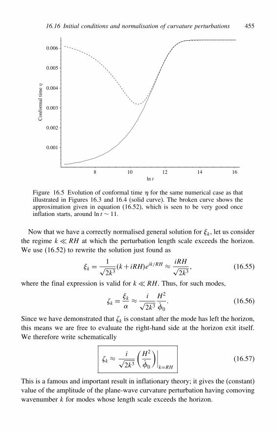
16.16 Initial conditions and normalisation of curvature perturbations 455
0.001
0.002
0.003
0.004
0.005
0.006
Con
form
al ti
me
η
8 10 12 14 16ln t
Figure 16.5 Evolution of conformal time for the same numerical case as thatillustrated in Figures 16.3 and 16.4 (solid curve). The broken curve shows theapproximation given in equation (16.52), which is seen to be very good onceinflation starts, around ln t ∼ 11.
Now that we have a correctly normalised general solution for k, let us considerthe regime k RH at which the perturbation length scale exceeds the horizon.We use (16.52) to rewrite the solution just found as
k =1√2k3
k+ iRHeik/RH ≈ iRH√2k3
(16.55)
where the final expression is valid for k RH . Thus, for such modes,
k =k≈ i√
2k3H2
0
(16.56)
Since we have demonstrated that k is constant after the mode has left the horizon,this means we are free to evaluate the right-hand side at the horizon exit itself.We therefore write schematically
k ≈i√2k3
(H2
0
)∣∣∣∣k=RH
(16.57)
This is a famous and important result in inflationary theory; it gives the (constant)value of the amplitude of the plane-wave curvature perturbation having comovingwavenumber k for modes whose length scale exceeds the horizon.
456 Inflationary cosmology
16.17 Power spectrum of curvature perturbations
From the result (16.57), we can deduce an expression for the power spectrumk of the primordial curvature perturbations. The precise definition of thisspectrum is a matter of convention, of which there are several, but we will adoptthe most commonly used. In this case, the power spectrum of a given spatiallyvarying field is defined as the contribution to the total variance of the field per unitlogarithmic interval in k. Thus, we define the curvature spectrum k such that
x∗x ≡∫
0kdln k (16.58)
where · · · denotes a expectation value and the total spatial variation of thecurvature perturbations is
x= 123/2
∫k expik · xd3k (16.59)
In these expressions, x refers to comoving coordinates and k = k. Evaluatingx∗x, and remembering that d3k = 4k2dk, one finds that (16.58) issatisfied providing that ⟨
k ∗k′⟩= 22
k3k
3(k−k′)where 3
(k−k′) is the three-dimensional delta function. We may therefore writek= k3k2/22 and, using (16.57), we finally obtain8
k=(
H2
20
)2
k=RH (16.60)
In the slow-roll approximation, we know that H is only slowly decreasingwhilst 0 is approximately constant. To a first approximation, therefore, thepower spectrum of the perturbations expected from inflation, as measured bythe contribution to the total fluctuation per unit logarithmic interval, is constant.Such a spectrum is called scale invariant and was proposed in the late 1960s asbeing the most likely to lead to structure appropriately distributed over the scaleswe see today. It is also known as a Harrison–Zel’dovich spectrum, after its twoco-proposers. Here we can see it emerging as a prediction of inflation. We cango further, however, by noting that, during inflation, H is slowly declining, 0
is approximately constant and R is increasing exponentially. Thus modes with
8 We note that the quantity k is often written using the alternative notation 2 k. In addition, it is common
to define the quantity Pk≡ k2, which is also often called the power spectrum and is related to k
by k= k3Pk/22.
16.17 Power spectrum of curvature perturbations 457
higher k, which leave the horizon later in time, have a slightly lower value ofk since H is lower there. As a result, the spectrum is predicted to be notexactly constant, but slightly declining, as a function of k. The details of thisdepend on the details of the potential V0, but we can see from the analysishere that this is a generic prediction of inflation (assuming that slow-roll is anaccurate model).
Before going on to discuss in the next section the comparison of the prediction(16.60) with cosmological observations, it is worthwhile re-deriving this resultin a more heuristic (and perhaps enlightening) manner. For a scalar field in anordinary Minkowski spacetime, the zero-point uncertainty fluctuation is given by
kp≈ 1
V 1/2
e−ikpt√2kp
(16.61)
for a mode with physical wavenumber kp, where V is a normalising volume. Here,instead of kp, we wish to use the comoving wavenumber k, which is related tothe physical wavenumber by k= Rkp. Moreover, an obvious length scale for thenormalising volume is the scale factor R. Thus, in our expanding FRW spacetime,we assume that
k ≈e−ikt/R
R√2k
(16.62)
As explained above, the corresponding power spectrum of the fluctuations k
is obtained by multiplying its squared norm by 4k3/23, which gives
k=(
k
2R
)2
k=RH=(H
2
)2
(16.63)
As above, we have evaluated the second expression at the ‘horizon crossing’value of k, RH , since fluctuations on larger length scales are ‘frozen in’ at thevalue they reached at this point. To translate this result into the power spectrumof curvature perturbations , we need to link and . Consider the change tin time coordinate that would be needed to move between the ‘comoving slicing’,in which vanishes, to a ‘flat slicing’, in which % vanishes. Since , as definedin (16.39), remains constant in this process, we see that, in this case,
% =% =−=Ht and = =−0t (16.64)
Eliminating t we find that =H/0 and hence we recover the result
k= k=(
H2
20
)2
k=RH (16.65)
458 Inflationary cosmology
16.18 Power spectrum of matter-density perturbations
As discussed in Section 16.6, at the end of inflation the scalar field decaysinto other particles. Thus, one is left with a spectrum of curvature perturbations,which from (16.40) is equivalent to the spectrum of fluctuations in the gravita-tional potential % in a comoving slicing. These in turn may be related to thecorresponding fluctuations in the matter density. The full general-relativisticequations describing the evolution under gravity of these density fluctuations maybe obtained by repeating all the above discussion for a perfect fluid rather thana scalar field. We will not pursue this calculation here but merely note that theresulting equations are the same as those obtained using Newtonian theory, exceptfor a term that is important only on super-horizon scales. Therefore, on sub-horizon scales, to a good approximation we may take these potential fluctuationsas obeying the perturbed Poisson’s equation in Newtonian gravity,
2%= 4G
where is the fluctuation in the matter density corresponding to that in thepotential. Indeed, we might have expected the Newtonian theory to be a goodapproximation on sub-horizon scales since the gravitational field associated withthe perturbations is weak.
It is more common to work instead in terms of the fractional-density fluctuation≡ /0, where 0 is the background matter density. Thus, working in Fourierspace, we have
%k =−4G0R
2
k2k
Using 0 = 3H2/8G, for the simple spatially flat case that we are consideringwe see that
k =−23
(k
RH
)2
%k (16.66)
from which we deduce that k2 ∝ k4%k2. Therefore, defining the matterpower spectrum by Pk≡ k2 (note that this differs from definition of k
by a factor k3/22, as mentioned earlier), we find that Pk∝ kk. Sincek is roughly constant for slow-roll inflation, we thus obtain
Pk∝ k (16.67)
In general, the matter power spectrum is parameterised as Pk∝ kn, where n isknown as the primordial spectral index. We therefore see that inflation naturallypredicts n= 1, which is also known as the Harrison–Zel’dovich spectrum.
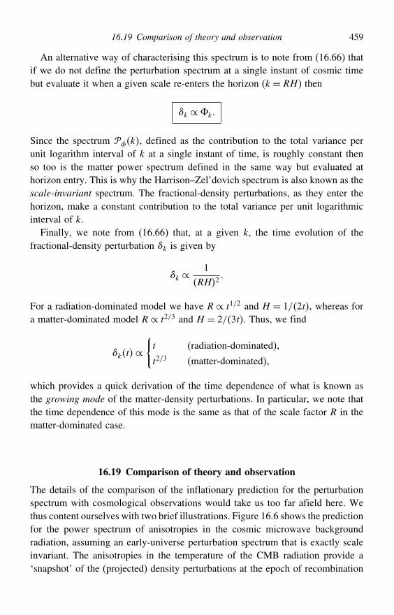
16.19 Comparison of theory and observation 459
An alternative way of characterising this spectrum is to note from (16.66) thatif we do not define the perturbation spectrum at a single instant of cosmic timebut evaluate it when a given scale re-enters the horizon (k= RH) then
k ∝%k
Since the spectrum k, defined as the contribution to the total variance perunit logarithm interval of k at a single instant of time, is roughly constant thenso too is the matter power spectrum defined in the same way but evaluated athorizon entry. This is why the Harrison–Zel’dovich spectrum is also known as thescale-invariant spectrum. The fractional-density perturbations, as they enter thehorizon, make a constant contribution to the total variance per unit logarithmicinterval of k.
Finally, we note from (16.66) that, at a given k, the time evolution of thefractional-density perturbation k is given by
k ∝1
RH2
For a radiation-dominated model we have R∝ t1/2 and H = 1/2t, whereas fora matter-dominated model R∝ t2/3 and H = 2/3t. Thus, we find
kt∝t (radiation-dominated)
t2/3 (matter-dominated)
which provides a quick derivation of the time dependence of what is known asthe growing mode of the matter-density perturbations. In particular, we note thatthe time dependence of this mode is the same as that of the scale factor R in thematter-dominated case.
16.19 Comparison of theory and observation
The details of the comparison of the inflationary prediction for the perturbationspectrum with cosmological observations would take us too far afield here. Wethus content ourselves with two brief illustrations. Figure 16.6 shows the predictionfor the power spectrum of anisotropies in the cosmic microwave backgroundradiation, assuming an early-universe perturbation spectrum that is exactly scaleinvariant. The anisotropies in the temperature of the CMB radiation provide a‘snapshot’ of the (projected) density perturbations at the epoch of recombination
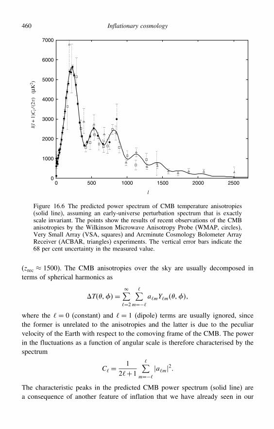
460 Inflationary cosmology
0
1000
2000
3000
4000
5000
6000
7000
0 500 1000 1500 2000 2500
l
l(l+
1)C
l/(2
π)(µ
K2 )
Figure 16.6 The predicted power spectrum of CMB temperature anisotropies(solid line), assuming an early-universe perturbation spectrum that is exactlyscale invariant. The points show the results of recent observations of the CMBanisotropies by the Wilkinson Microwave Anisotropy Probe (WMAP, circles),Very Small Array (VSA, squares) and Arcminute Cosmology Bolometer ArrayReceiver (ACBAR, triangles) experiments. The vertical error bars indicate the68 per cent uncertainty in the measured value.
(zrec ≈ 1500). The CMB anisotropies over the sky are usually decomposed interms of spherical harmonics as
T=∑=2
∑m=−
amYm
where the = 0 (constant) and = 1 (dipole) terms are usually ignored, sincethe former is unrelated to the anisotropies and the latter is due to the peculiarvelocity of the Earth with respect to the comoving frame of the CMB. The powerin the fluctuations as a function of angular scale is therefore characterised by thespectrum
C =1
2+1
∑m=−
am2
The characteristic peaks in the predicted CMB power spectrum (solid line) area consequence of another feature of inflation that we have already seen in our
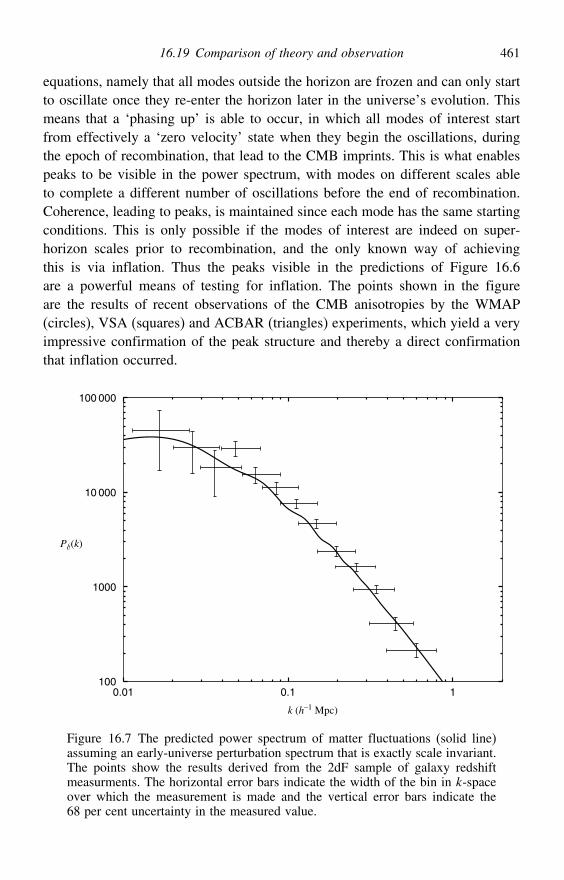
16.19 Comparison of theory and observation 461
equations, namely that all modes outside the horizon are frozen and can only startto oscillate once they re-enter the horizon later in the universe’s evolution. Thismeans that a ‘phasing up’ is able to occur, in which all modes of interest startfrom effectively a ‘zero velocity’ state when they begin the oscillations, duringthe epoch of recombination, that lead to the CMB imprints. This is what enablespeaks to be visible in the power spectrum, with modes on different scales ableto complete a different number of oscillations before the end of recombination.Coherence, leading to peaks, is maintained since each mode has the same startingconditions. This is only possible if the modes of interest are indeed on super-horizon scales prior to recombination, and the only known way of achievingthis is via inflation. Thus the peaks visible in the predictions of Figure 16.6are a powerful means of testing for inflation. The points shown in the figureare the results of recent observations of the CMB anisotropies by the WMAP(circles), VSA (squares) and ACBAR (triangles) experiments, which yield a veryimpressive confirmation of the peak structure and thereby a direct confirmationthat inflation occurred.
100
1000
10 000
100 000
0.01 0.1 1
k (h–1 Mpc)
Pδ (k)
Figure 16.7 The predicted power spectrum of matter fluctuations (solid line)assuming an early-universe perturbation spectrum that is exactly scale invariant.The points show the results derived from the 2dF sample of galaxy redshiftmeasurments. The horizontal error bars indicate the width of the bin in k-spaceover which the measurement is made and the vertical error bars indicate the68 per cent uncertainty in the measured value.
462 Inflationary cosmology
From the current data it is, however, not possible to tell whether the primordialspectrum is exactly scale invariant, as assumed in generating the prediction, orwhether it has the slight decrease at larger k, and therefore smaller scales, that wesaid was also a generic prediction of inflation. This question should be resolved byfuture experimental results, particularly from the CMB on smaller angular scalesand from measurements of the matter distribution on a range of scales. In thelatter case, one may compare the observed distribution of galaxies (both over thesky and in redshift) with the predicted power spectrum for matter fluctuations inthe universe. The primordial matter power spectrum Pk in (16.67) is modifiedby the evolution under gravity of the perturbations once they re-enter the horizon.This effect may be calculated, and the predicted matter power spectrum resultingfrom an exactly scale-invariant primordial spectrum from inflation is shown asthe solid line in Figure 16.7. Once again, we see that the predicted spectrumhas oscillations resulting from an mechanism analogous to that which producesthe oscillations in the CMB power spectrum discussed above. The points in thefigure show the measurements derived from the 2dF (2 degree field) sample ofgalaxy redshift measurments. Again, a good fit to the data is visible, and timewill tell whether the detailed dynamics of inflation, which can be measured by thedepartures from scale invariance, will become accessible from the combinationof data of this type and future CMB experiments.
Exercises
16.1 In the cosmological field equation
R2 = 13R
2−k
show that, if p < − 13, the curvature term becomes negligible as the universe
expands.16.2 Show that the energy–momentum tensor of a scalar field,
T = −g[12 #
#−V]
satisfies the condition T = 0.
16.3 Show that a scalar field acts like a perfect fluid with an energy density and pressuregiven by
= 12
2+V+ 12 2
p = 12
2−V− 16 2
Show further that if the field is spatially constant then inflation will occur,provided that 2 < V. If, in addition, the scalar field does not change with time,show that its equation of state is p = − and that it thus acts as an effectivecosmological constant.
Exercises 463
16.4 Show that the equation of motion for a scalar field with potential V is
+3H+ dV
d= 0
Hence find the general solution for a free scalar field , for which V = 12m
22, inthe case where H is approximately constant.
16.5 For a potential of the form
V= V0 exp−where is a positive constant, show that the inflation equations can be solvedexactly to give
Rt= R0
(t
t0
)2/2
t= 0+2ln
(√V0
26−22t
)
Hence show that, provided <√2, the solution corresponds to a period of inflation.
Show further that the slow-roll parameters for this model are = 12= 1
22, and so
the inflationary epoch never ends. This model is known as power-law inflation.16.6 Show that, in general,
R= RH+H2
Show that H > 0 only if p <−, which is forbidden by the weak energy condition(see Exercise 8.8). Hence show that, for inflation to occur, one requires
− H
H2< 1
and thus that the first slow-roll parameter must obey < 1.16.7 In the slow-roll approximation, show that
H =− 12
2
Assuming that varies monotonically with t throughout the period of inflation,show that
=−2H ′
where H is now considered as a function of , and hence that we may write thecosmological field equation as
H ′2− 32H
2=− 12V
This is known as the Hamilton–Jacobi formalism for inflation.16.8 Repeat Exercise 16.5 using the Hamilton–Jacobi formalism developed in Exer-
cise 16.7.
464 Inflationary cosmology
16.9 In the Hamilton–Jacobi formalism developed in Exercise 16.7, show that thecondition for inflation to occur is
2[H ′H
]2< 1
16.10 Show that, during an exponential expansion phase of the universe, the properdistance between any two comoving objects separated by more than H−1 growsat a speed exceeding the speed of light. Hence show that an observer in such auniverse can only see processes occurring inside the ‘horizon’ radius H−1, and sothe process of inflation in any spatial domain of radius H−1 (or ‘mini-universe’)occurs independently of any events outside it.
16.11 A fluctuation in the scalar inflation field leads to a local delay of the end ofinflation by t ∼ /. Assuming that the density of the universe after inflationdecreases as t−2, show that the fluctuation in the scalar field leads to a relativedensity contrast at the end of inflation given by
∼ H
Assuming the root mean square (rms) scalar field perturbation to be rms ∼H/2, show that (
)rms
∼ H2
2
16.12 Consider an inflationary domain (or mini-universe in the context of Exercise 16.10)of initial radius H−1, in which the value of the scalar field 1. In a time intervalt = H−1, show that classically, in the slow-roll approximation, the value of will change by
≈− 2
Assuming that the typical amplitude of quantum fluctuations in the scalar field is≈H/2, show that
≈ 12
√V
3
Hence, for the case V= 12m
22, show that the decrease in the value of the scalarfield due to its classical motion is less than changes due to quantum fluctuationsgenerated in the same time interval, provided that
6√m
Assuming that the typical wavelength of the quantum fluctuation is is H−1,show that, after a time interval t=H−1, the original domain becomes effectivelydivided into e3 ∼ 20 domains of radius H−1, each containing a roughly homoge-neous scalar field ++ . Thus, on average, the volume of the universe
Exercises 465
containing a growing -field increases by a factor ∼ 10 after every time intervalt =H−1.Note: This is the mechanism underlying stochastic inflation.
16.13 For the line element
ds2 = 1+2% dt2− 1−2%R2tdx2+dy2+dz2
show that, to first order in %, the perturbed parts of the connection coefficientstake the form
00 = %
0ii = −R2%+4H%
i00 =
1R2
i%
ii = −%
where no sum over repeated i indices is implied and and the remaining perturbedcoefficients either follow from symmetry or are zero. Hence show that theperturbed part of the Einstein tensor is given by
G0i = −2i%+H%
G00 = −22%−3H%−3H2%
Gii = 2 %+4%H+ 2H+3H2%
where again no sum over repeated i indices is implied and the remaining entrieseither follow from symmetry or are zero.
16.14 For the scalar-field perturbation
t→ 0t+t xshow that, to first order in , the perturbed parts of the scalar-field energy–momentum tensor are given by
T 0i = 0i
T 00 = −2
0%+ 0+V ′
T ii = 2
0%− 0+V ′
where V ′ = dV/d0 and the remaining components either follow from symmetryor are zero.
16.15 Use your answers to Exercises 16.13 and 16.14 to show that the perturbed Einsteinfield equations yield only the two equations
%+H% = 120(
20+22
)% = 2
0
d
dt
(
0
)
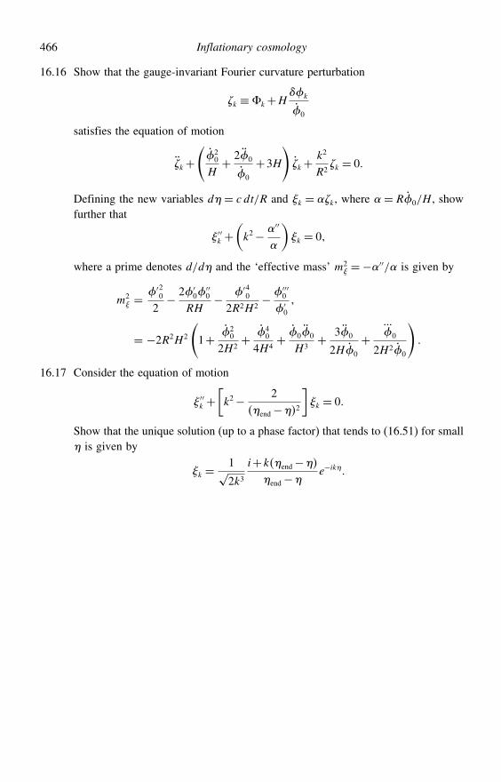
466 Inflationary cosmology
16.16 Show that the gauge-invariant Fourier curvature perturbation
k ≡%k+Hk
0
satisfies the equation of motion
k+(2
0
H+ 20
0
+3H
)k+
k2
R2k = 0
Defining the new variables d= c dt/R and k = k, where = R0/H , showfurther that
′′k +(k2− ′′
)k = 0
where a prime denotes d/d and the ‘effective mass’ m2 =−′′/ is given by
m2 =
′202− 2′0
′′0
RH− ′40
2R2H2− ′′′0
′0
= −2R2H2
(1+ 2
0
2H2+ 4
0
4H4+ 00
H3+ 30
2H0
+...0
2H20
)
16.17 Consider the equation of motion
′′k +[k2− 2
end−2
]k = 0
Show that the unique solution (up to a phase factor) that tends to (16.51) for small is given by
k =1√2k3
i+kend−
end−e−ik
17
Linearised general relativity
The gravitational field equations give a quantitative description of how the curva-ture of spacetime at any event is related to the energy–momentum distribution atthat event. The high degree of non-linearity in these field equations means thata general solution for an arbitrary matter distribution is analytically intractable.Consequently, thus far we have concentrated primarily on investigating a numberof special solutions that represent spacetimes with particular symmetries (asidefrom our discussion of perturbations in the previous chapter). In this chapter,we return to a more general investigation of the gravitational field equations andtheir solutions. To enable such a study, however, one must make the physicalassumption that the gravitational fields are weak. Mathematically, this assumptioncorresponds to linearising the gravitational field equations.
17.1 The weak-field metric
As discussed in Sections 7.6 and 8.6, a weak gravitational field corresponds to aregion of spacetime that is only ‘slightly’ curved. Thus, throughout such a region,there exist coordinate systems x in which the spacetime metric takes the form
g = +h where h 1 (17.1)
and the first and higher partial derivatives of h are also small.1 Such coordinatesare often termed quasi-Minkowskian coordinates, since they allow the metricto be written in a close-to-Minkowski form. Clearly, h must be symmetricwith respect to the swapping of its indices. We also note that, when previously
1 We note that one could equally well consider small perturbations about some other background metric, suchthat g = g
0 +h . This was the case in our discussion of inflationary perturbations in the previous chapter,
in which g0 was the metric for the background Friedmann–Robertson–Walker spacetime in comoving
Cartesian coordinates.
467
468 Linearised general relativity
considering the weak-field limit, we further assumed that the metric was stationary,so that 0g = 0h = 0 where x0 is the timelike coordinate. In our presentdiscussion, however, we wish to retain the possibility of describing time-varyingweak gravitational fields, and so we shall notmake this additional assumption here.
As we have stressed many times, coordinates are arbitrary and, in principle,one could develop the description of weak gravitational fields in any coordinatesystem. Nevertheless, by adopting quasi-Minkowsian coordinates the mathemati-cal labour of pursuing our analysis is greatly simplified, as is the interpretation ofthe resulting expressions. If one coordinate system exists in which (17.1) holds,however, then there must be many such coordinate systems. Indeed, two differ-ent types of coordinate transformation connect quasi-Minkowskian systems toeach other: global Lorentz transformations and infinitesimal general coordinatetransformations, both of which we now discuss.
Global Lorentz transformations
Global Lorentz transformations are of the form
x′ =$x
where =$$
##
and the quantities $ are constant everywhere. These transform the metric
coefficients as follows:
g′ =x
x′x#
x′g# =$
$## +h#= +$
$#h#
Thus, g′ is also of the form (17.1), with
h′ =$$
#h#
Moreover, we see from this expression that, under a Lorentz transformation, hitself transforms like the components of a tensor in Minkowski spacetime.
The above property suggests a convenient alternative viewpoint when describ-ing weak gravitational fields. Instead of considering a slightly curved spacetimerepresenting the general-relativistic weak field, we can consider h simply as asymmetric rank-2 tensor field defined on the flat Minkowski background space-time in Cartesian inertial coordinates. In other words, h is considered as aspecial-relativistic gravitational field, in an analogous way to that in which the4-potential A describes the electromagnetic field in Minkowski spacetime, asdiscussed in Chapter 6; we return to this point below. We note, however, thath does not transform as a tensor under a general coordinate transformation butonly under the restricted class of global Lorentz transformations; for this reasonh and tensors derived from it are sometimes called pseudotensors, although wewill not use this terminology.
17.1 The weak-field metric 469
Infinitesimal general coordinate transformations
Infinitesimal general coordinate transformations take the form
x′ = x+x (17.2)
where the x are four arbitrary functions of position of the same order ofsmallness as the h. Infinitesimal transformations of this sort make tiny changesin the forms of all scalar, vector and tensor fields, but these can be ignored inall quantities except the metric, where tiny deviations from contain all theinformation about gravity. From (17.2), we have
x′
x= +
and, working to first order in small quantities, it is straightforward to show thatthe inverse transformation is given by2
x
x′= −
(17.3)
Thus, again working to first order in small quantities, the metric transforms asfollows:
g′ =x
x′x#
x′g# = −
# − ## +h#
= +h− −
where we have defined = . Hence, we see that g′ is also of the form
(17.1), the new metric perturbation functions being related to the old ones via
h′ = h− − (17.4)
If we adopt the viewpoint in which h is considered as a tensor field definedon the flat Minkowski background spacetime, then (17.4) can be consideredas analogous to a gauge transformation in electromagnetism. As discussed inChapter 6, if A is a solution of the electromagnetic field equations then anothersolution that describes precisely the same physical situation is given by
Anew = A+
where is any scalar field. An analogous situation holds in the case of thegravitational field. From (17.4), it is clear that if h is a solution to the linearised
2 Note that, for the remainder of this chapter, the normal symbol for equality will be used to indicate equalityup to first order in small quantities as well as exact equality.
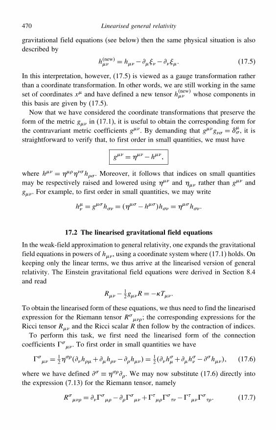
470 Linearised general relativity
gravitational field equations (see below) then the same physical situation is alsodescribed by
hnew = h− − (17.5)
In this interpretation, however, (17.5) is viewed as a gauge transformation ratherthan a coordinate transformation. In other words, we are still working in the sameset of coordinates x and have defined a new tensor hnew whose components inthis basis are given by (17.5).
Now that we have considered the coordinate transformations that preserve theform of the metric g in (17.1), it is useful to obtain the corresponding form forthe contravariant metric coefficients g. By demanding that gg# =
# , it is
straightforward to verify that, to first order in small quantities, we must have
g = −h
where h = #h# . Moreover, it follows that indices on small quantitiesmay be respectively raised and lowered using and rather than g andg. For example, to first order in small quantities, we may write
h = g#h# = # −h#h# = #h#
17.2 The linearised gravitational field equations
In the weak-field approximation to general relativity, one expands the gravitationalfield equations in powers of h, using a coordinate system where (17.1) holds. Onkeeping only the linear terms, we thus arrive at the linearised version of generalrelativity. The Einstein gravitational field equations were derived in Section 8.4and read
R− 12gR=−&T
To obtain the linearised form of these equations, we thus need to find the linearisedexpression for the Riemann tensor R#
; the corresponding expressions for theRicci tensor R and the Ricci scalar R then follow by the contraction of indices.
To perform this task, we first need the linearised form of the connectioncoefficients #
. To first order in small quantities we have
# = 1
2#h+ h− h= 1
2h#+ h
# − #h (17.6)
where we have defined # ≡ #. We may now substitute (17.6) directly intothe expression (7.13) for the Riemann tensor, namely
R# =
#−
#+
#−
# (17.7)
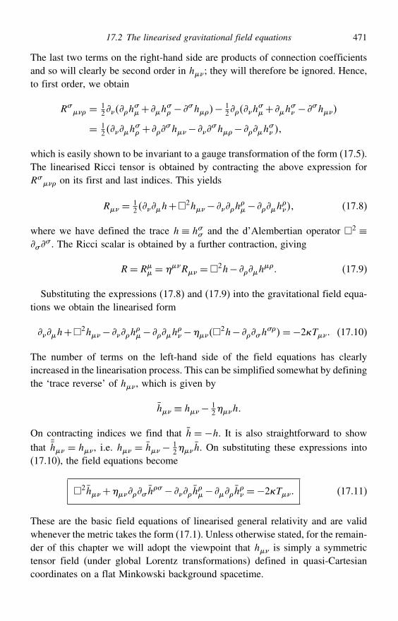
17.2 The linearised gravitational field equations 471
The last two terms on the right-hand side are products of connection coefficientsand so will clearly be second order in h; they will therefore be ignored. Hence,to first order, we obtain
R# = 1
2h#+ h
# − #h− 1
2h#+ h
# − #h
= 12h
# +
#h− #h− h
#
which is easily shown to be invariant to a gauge transformation of the form (17.5).The linearised Ricci tensor is obtained by contracting the above expression forR#
on its first and last indices. This yields
R = 12h+2h− h
− h
(17.8)
where we have defined the trace h ≡ h## and the d’Alembertian operator 2 ≡#
# . The Ricci scalar is obtained by a further contraction, giving
R= R = R =2h− h
(17.9)
Substituting the expressions (17.8) and (17.9) into the gravitational field equa-tions we obtain the linearised form
h+2h− h− h
−2h− #h
#=−2&T (17.10)
The number of terms on the left-hand side of the field equations has clearlyincreased in the linearisation process. This can be simplified somewhat by definingthe ‘trace reverse’ of h, which is given by
h ≡ h− 12h
On contracting indices we find that h = −h. It is also straightforward to showthat ¯h = h, i.e. h = h− 1
2h. On substituting these expressions into(17.10), the field equations become
2h+#h# − h
− h
=−2&T (17.11)
These are the basic field equations of linearised general relativity and are validwhenever the metric takes the form (17.1). Unless otherwise stated, for the remain-der of this chapter we will adopt the viewpoint that h is simply a symmetrictensor field (under global Lorentz transformations) defined in quasi-Cartesiancoordinates on a flat Minkowski background spacetime.
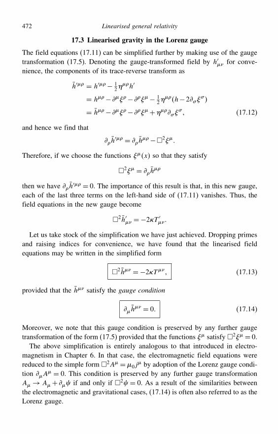
472 Linearised general relativity
17.3 Linearised gravity in the Lorenz gauge
The field equations (17.11) can be simplified further by making use of the gaugetransformation (17.5). Denoting the gauge-transformed field by h′ for conve-nience, the components of its trace-reverse transform as
h′ = h′− 12
h′
= h− − − 12
h−2##
= h− − +## (17.12)
and hence we find that
h′ = h
−2
Therefore, if we choose the functions x so that they satisfy
2 = h
then we have h′ = 0. The importance of this result is that, in this new gauge,
each of the last three terms on the left-hand side of (17.11) vanishes. Thus, thefield equations in the new gauge become
2h′ =−2&T ′Let us take stock of the simplification we have just achieved. Dropping primes
and raising indices for convenience, we have found that the linearised fieldequations may be written in the simplified form
2h =−2&T (17.13)
provided that the h satisfy the gauge condition
h = 0 (17.14)
Moreover, we note that this gauge condition is preserved by any further gaugetransformation of the form (17.5) provided that the functions satisfy 2 = 0.The above simplification is entirely analogous to that introduced in electro-
magnetism in Chapter 6. In that case, the electromagnetic field equations werereduced to the simple form 2A =0j
by adoption of the Lorenz gauge condi-tion A
= 0. This condition is preserved by any further gauge transformationA → A+ if and only if 2 = 0. As a result of the similarities betweenthe electromagnetic and gravitational cases, (17.14) is often also referred to as theLorenz gauge.
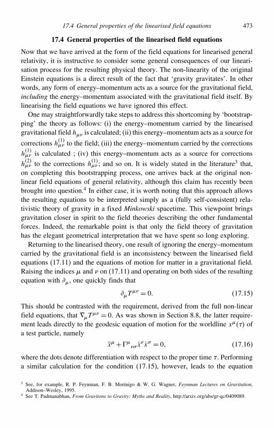
17.4 General properties of the linearised field equations 473
17.4 General properties of the linearised field equations
Now that we have arrived at the form of the field equations for linearised generalrelativity, it is instructive to consider some general consequences of our lineari-sation process for the resulting physical theory. The non-linearity of the originalEinstein equations is a direct result of the fact that ‘gravity gravitates’. In otherwords, any form of energy–momentum acts as a source for the gravitational field,including the energy–momentum associated with the gravitational field itself. Bylinearising the field equations we have ignored this effect.
One may straightforwardly take steps to address this shortcoming by ‘bootstrap-ping’ the theory as follows: (i) the energy–momentum carried by the linearisedgravitational field h is calculated; (ii) this energy–momentum acts as a source for
corrections h1 to the field; (iii) the energy–momentum carried by the corrections
h1 is calculated ; (iv) this energy–momentum acts as a source for corrections
h2 to the corrections h1 ; and so on. It is widely stated in the literature3 that,
on completing this bootstrapping process, one arrives back at the original non-linear field equations of general relativity, although this claim has recently beenbrought into question.4 In either case, it is worth noting that this approach allowsthe resulting equations to be interpreted simply as a (fully self-consistent) rela-tivistic theory of gravity in a fixed Minkowski spacetime. This viewpoint bringsgravitation closer in spirit to the field theories describing the other fundamentalforces. Indeed, the remarkable point is that only the field theory of gravitationhas the elegant geometrical interpretation that we have spent so long exploring.
Returning to the linearised theory, one result of ignoring the energy–momentumcarried by the gravitational field is an inconsistency between the linearised fieldequations (17.11) and the equations of motion for matter in a gravitational field.Raising the indices and on (17.11) and operating on both sides of the resultingequation with , one quickly finds that
T = 0 (17.15)
This should be contrasted with the requirement, derived from the full non-linearfield equations, that T
= 0. As was shown in Section 8.8, the latter require-ment leads directly to the geodesic equation of motion for the worldline x ofa test particle, namely
x+ #x
x# = 0 (17.16)
where the dots denote differentiation with respect to the proper time . Performinga similar calculation for the condition (17.15), however, leads to the equation
3 See, for example, R. P. Feynman, F. B. Morinigo & W. G. Wagner, Feynman Lectures on Gravitation,Addison–Wesley, 1995.
4 See T. Padmanabhan, From Gravitons to Gravity: Myths and Reality, http://arxiv.org/abs/gr-qc/0409089.
474 Linearised general relativity
of motion x = 0, which means that the gravitational field has no effect on themotion of the particle. In general, this clearly contradicts the geodesic postulate.
An alternative way to uncover this inconsistency is to note that an immediateconsequence of having linearised the field equations is that solutions can be added.In other words, if the pairs of tensors hi and Ti individually satisfy (17.11)for i = 12 then the quantity
∑ihi is also a solution, corresponding to
the energy–momentum tensor∑
iTi. Thus, for example, two point massescould remain at a fixed separation from one another indefinitely, the resultinggravitational field being simply the superposition of their individual radial fields.
Despite this inconsistency, linearised general relativity is still a useful approx-imation, provided that we are interested only in the far field of sources whosemotion we know a priori and that we are willing to neglect the ‘gravity of grav-ity’. In such cases, the effect of weak gravitational fields on test particles canbe computed by inserting the form (17.6) for the connection coefficients into thegeodesic equations (17.16). To calculate how the sources themselves move undertheir own gravity, however, one would need to re-insert into the field equationsthe non-linear terms that the linear theory discards.
17.5 Solution of the linearised field equations in vacuo
In empty space, the linearised field equations in the Lorenz gauge reduce to thewave equation
2h = 0 (17.17)
with the attendant gauge condition
h = 0 (17.18)
It is straightforward to show that the field equations have plane-wave solutionsof the form
h = A expikx (17.19)
where the A are constant (and, in general, complex) components of a symmetrictensor, and the k are the constant (real) components of a vector. Substitutingthe expression (17.19) into the wave equation (17.17) and using the fact thath
= kh, we find that
2h = ##h = #kk#h
= 0
This can only be satisfied if
#kk# = k#k# = 0 (17.20)
17.6 General solution of the linearised field equations 475
and hence the vector k must be null. Since the linearised Einstein equations onlytake the simple form (17.17) in the Lorenz gauge, we must also take into accountthe gauge condition (17.18). On substituting into the latter the plane-wave form(17.19), we immediately find that the gauge condition is satisfied provided thatone obeys the additional constraint
Ak = 0 (17.21)
Thus any plane wave of the form (17.19) is a valid solution of the linearisedvacuum field equations in the Lorenz gauge, provided that the vector k satisfies(17.20) and (17.21). We will discuss plane gravitational waves in detail in thenext chapter.
Since the vacuum field equations are linear (by design), any solution of themmay be written as a superposition of such plane-wave solutions of the form
hx=∫Ak expikxd3k (17.22)
where k = k0 k and the integral is taken over all values of k. Physicalsolutions are obtained by taking the real part of (17.22).
17.6 General solution of the linearised field equations
We now consider the general form of the solution to the linearised field equationsin the presence of some non-zero energy–momentum tensor T. In this case,the field equations take the form of an inhomogeneous wave equation for eachcomponent,
2h =−2&T (17.23)
together with the attendant gauge condition h = 0. The general solution to
(17.23) is most easily obtained by using a Green’s function, in a similar mannerto that employed for solving the analogous problem in electromagnetism. We willnow outline this approach.
One begins by considering the solution to the inhomogeneous wave equationwhen the source is a -function, i.e. it is located at a definite event in spacetime.If this event has coordinates y# , one is therefore interested in solving an equationof the form
2xGx# −y#= 4x# −y# (17.24)
where the subscript on 2x makes explicit that the d’Alembertian operator is with
respect to the coordinates x# and Gx# − y# is the Green’s function for ourproblem, which in the absence of boundaries must be a function only of thedifference x# − y# . Since the field equations (17.23) are linear, sources that are
476 Linearised general relativity
more general can be built up by adding further -function sources located atdifferent events. Thus, the general solution to the linearised field equations canbe written5
hx#= h0x
#−2&∫Gx# −y#Ty#d4y (17.25)
where, for completeness, we have made use of the freedom to add any solutionh0x of the homogeneous field equations (i.e. the in vacuo field equations). It
may be verified immediately by direct substitution that (17.25) does indeed solve(17.23). For the discussions in this chapter, however, we will take h
0x = 0
without loss of generality.The problem of obtaining a general solution of the linearised field equations has
thus been reduced to solving (17.24) to obtain the appropriate Green’s function.This may be achieved in a number of ways, and here we shall take a physicallymotivated approach. For convenience, we begin by placing the -function sourceat the origin of our coordinate system. We will also make the identifications x= ct x and r = x. With the source at the origin, we may write (17.24) as
Gx#= 4x# (17.26)
We first integrate this equation over a four-dimensional hypervolume V . Sincethe spatial spherical symmetry of the problem suggests that the Green’s functionshould only depend on ct and r, we choose the hypervolume to be a sphere ofradius r in its spatial dimensions and we integrate in t from − to . Thegeometry of the bounding surface S of the hypervolume is illustrated by thevertical cylinder in Figure 17.1, in which the third spatial dimension x3 has beensuppressed. Performing the integration of (17.26) over V we obtain∫
V
Gx#d4x =∫S Gx#n dS = 1 (17.27)
where in the first equality we have used the divergence theorem to rewrite thevolume integral as an integral over the bounding surface S with unit normal n.Since we are working with a metric of signature +−−−, it should be notedthat n is chosen to be outward pointing if it is timelike and inward pointing ifspacelike.
Let us now consider the contributions to this surface integral over S. Sincegravitational field variations travel at speed c, the only points in spacetime thatcan be influenced by a -function source at the origin are those lying on the
5 Note that there is no need to include√−g factors in our integral or delta-function definition, since we are
considering the problem simply as a tensor field hx defined on a Minkowski spacetime background in aCartesian coordinate system.
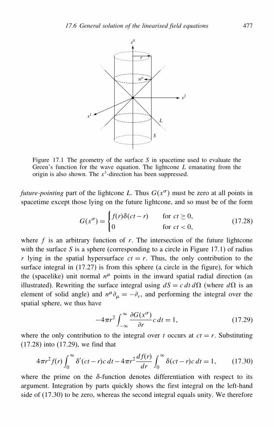
17.6 General solution of the linearised field equations 477
x1
x2
x0
r
L
S
nµ
Figure 17.1 The geometry of the surface S in spacetime used to evaluate theGreen’s function for the wave equation. The lightcone L emanating from theorigin is also shown. The x3-direction has been suppressed.
future-pointing part of the lightcone L. Thus Gx# must be zero at all points inspacetime except those lying on the future lightcone, and so must be of the form
Gx#=frct− r for ct ≥ 0
0 for ct < 0(17.28)
where f is an arbitrary function of r. The intersection of the future lightconewith the surface S is a sphere (corresponding to a circle in Figure 17.1) of radiusr lying in the spatial hypersurface ct = r. Thus, the only contribution to thesurface integral in (17.27) is from this sphere (a circle in the figure), for whichthe (spacelike) unit normal n points in the inward spatial radial direction (asillustrated). Rewriting the surface integral using dS = c dt d (where d is anelement of solid angle) and n = −r , and performing the integral over thespatial sphere, we thus have
−4r2∫
−Gx#
rc dt = 1 (17.29)
where the only contribution to the integral over t occurs at ct = r. Substituting(17.28) into (17.29), we find that
4r2fr∫
0′ct− rc dt−4r2
dfr
dr
∫
0ct− rc dt = 1 (17.30)
where the prime on the -function denotes differentiation with respect to itsargument. Integration by parts quickly shows the first integral on the left-handside of (17.30) to be zero, whereas the second integral equals unity. We therefore
478 Linearised general relativity
require −4r2df/dr = 1 and so fr= 1/4r, where the constant of integrationvanishes since the Green’s function must tend to zero at spatial infinity. Thus,re-expressing the result in terms of the coordinates x# , the required Green’sfunction is
Gx#= x0−x4x x0
where the Heaviside function x0 equals unity if x0 ≥ 0 and zero if x0 < 0.We may now use this form to substitute for Gx# − y# in (17.25), with h
0
set to zero, to obtain
hx#=− &
2
∫ (x0−y0−x−y)
x−y x0−y0Ty#d4y
Using the delta function to perform the integral over y0, we finally find that thegeneral solution to the linearised field equations (17.23) is given by
hct x=−4Gc4
∫ Tct−x−y yx−y d3y (17.31)
The interpretation of (17.31) requires some words of explanation. Here x repre-sents the spatial coordinates of the field point at which h is determined, yrepresents the spatial coordinates of a point in the source and x−y is the spatialdistance between them. We see that the disturbance in the gravitational field at theevent ct x is the integral over the region of spacetime occupied by the pointsof the source at the retarded times tr given by
ctr = ct−x−yThis region is the intersection of the past lightcone of the field point with theworld tube of the source. An illustration of the geometric meaning of the retardedtime is shown in Figure 17.2.
Although we have shown that (17.31) satisfies the linearised field equations(17.23), this form of the field equations is only valid in the Lorenz gauge. We musttherefore verify that (17.31) also satisfies the Lorenz gauge condition h
= 0.Before embarking on this we first remind ourselves how to differentiate a functionof retarded time. Setting x0r ≡ ctr = x0−x−y, for any function f we have
f(x0r y
)x
=[fy0 y
y0
]r
x0rx
(17.32)
f(x0r y
)yi
=[fy0 y
yi
]r+[fy0 y
y0
]r
x0ryi
(17.33)
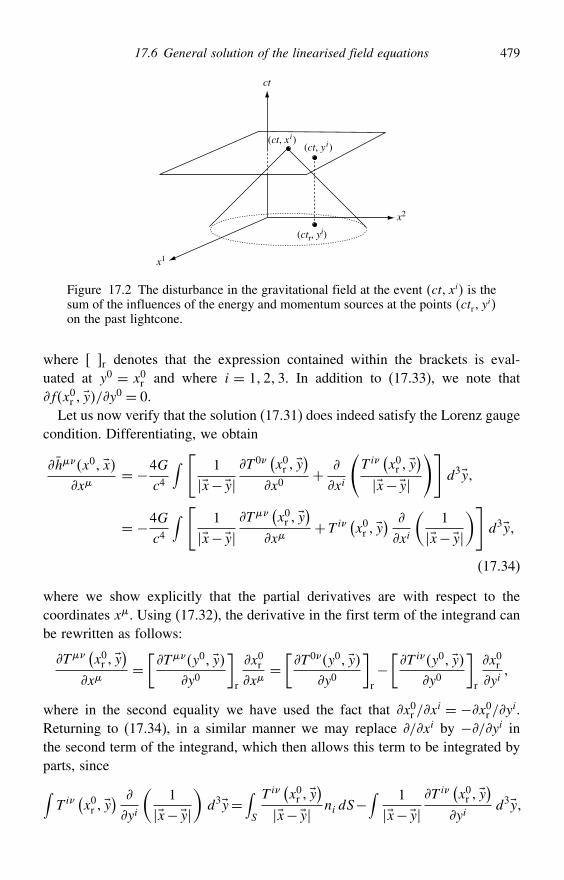
17.6 General solution of the linearised field equations 479
x2
x1
ct
(ct, xi)(ct, yi)
(ctr, yi)
Figure 17.2 The disturbance in the gravitational field at the event ct xi is thesum of the influences of the energy and momentum sources at the points ctr y
ion the past lightcone.
where r denotes that the expression contained within the brackets is eval-uated at y0 = x0r and where i = 123. In addition to (17.33), we note thatfx0r y/y0 = 0.
Let us now verify that the solution (17.31) does indeed satisfy the Lorenz gaugecondition. Differentiating, we obtain
hx0 xx
= −4Gc4
∫ [ 1
x−yT 0
(x0r y
)x0
+
xi
(T i
(x0r y
)x−y
)]d3y
= −4Gc4
∫ [ 1
x−yT
(x0r y
)x
+T i(x0r y
)
xi
(1
x−y)]
d3y
(17.34)
where we show explicitly that the partial derivatives are with respect to thecoordinates x. Using (17.32), the derivative in the first term of the integrand canbe rewritten as follows:
T(x0r y
)x
=[Ty0 y
y0
]r
x0rx
=[T 0y0 y
y0
]r−[T iy0 y
y0
]r
x0ryi
where in the second equality we have used the fact that x0r /xi = −x0r /yi.
Returning to (17.34), in a similar manner we may replace /xi by −/yi inthe second term of the integrand, which then allows this term to be integrated byparts, since∫T i
(x0r y
)
yi
(1
x−y)d3y=
∫S
T i(x0r y
)x−y ni dS−
∫ 1
x−yT i
(x0r y
)yi
d3y
480 Linearised general relativity
where S is the surface of the region of intersection between the past lightcone ofthe field point and the world tube of the source and ni is the outward-pointingnormal to the surface. Moreover, since T i
(x0r y
)vanishes on S, the surface
integral is zero.Combining our results, we may therefore write (17.34) as
h
x=−4G
c4
∫ [T 0(y0 y)
y0
]r
−[T iy0 y
y0
]r
x0ryi
+ T i(x0r y
)yi
d3yx−y
Making use of the result (17.33) to combine the last two terms within the braces,we thus arrive at the final form
h
x=−4G
c4
∫ 1
x−y[Ty0 y
y
]rd3y (17.35)
As shown in Section 17.4, however, in the linearised theory the energy–momentumtensor obeys T
= 0. Thus the integrand in (17.35) vanishes, and so we haveverified that the solution (17.31) satisfies the Lorenz gauge condition h
= 0.
17.7 Multipole expansion of the general solution
In general, the source of the gravitational field may be dynamic and have a spatialextent that is not small compared with the distance to the point at which onewishes to calculate the field. In such cases, obtaining a simple expression for thesolution (17.31) is often analytically intractable. In an analogous manner to thatused in electromagnetism, it is often convenient to perform a multipole expansionof (17.31), which lends itself to the calculation of successive approximations tothe solution. One begins by writing down the Taylor expansion
1
x−y =1r+ −yii
(1r
)+ 1
2!−yi−yjij
(1r
)+· · ·
= 1r+yi
xir3+yiyj
(3xixj− r2ij
r5
)+· · ·
where r ≡ x is the spatial distance from the origin to the field point and i ≡/xi. One may then write the solution (17.31) as
hct x = −4Gc4
[1r
∫Tctr yd3y+ xi
r3
∫Tctr yyi d3y
+ 3xixj− r2ij
r5
∫Tctr yyiyj d3y+· · ·
] (17.36)
17.8 The compact-source approximation 481
where ctr = ct−x−y. This multipole expansion may be written in a particularlycompact form:
hct x=−4Gc4
∑=0
−1! Mi1i2···ictri1i2 · · · i
(1r
)
where the multipole moments of the source distribution at any time t are given by
Mi1i2···ict=∫Tct yyi1yi2 · · ·yi d3y
Since the fall-off with distance of the term associated with the th multipolemoment goes as 1/r+1, the gravitational field at large distances from the sourceis well approximated by only the first few terms of the multipole expansion.
17.8 The compact-source approximation
Let us suppose that the source is some matter distribution localised near the originO of our coordinate system. If we take our field point x to be a distance r fromO that is large compared with the spatial extent of the source, we need consideronly the first term in the multipole expansion (17.36). Moreover, we assume thatthe source particles have speeds that are sufficiently small compared with c for usto take ctr = ct− r in the argument of the stress–energy tensor. Thus, the solutionin the compact-source approximation is given by
hct x=−4Gc4r
∫Tct− r yd3y (17.37)
In this approximation, we are thus considering only the far-field solution to thelinearised gravitational equations, which varies as 1/r.
From (17.37), we see that calculating the gravitational field has been reducedto integrating T over the source at a fixed retarded time ct− r. The physicalinterpretation of the various components of this integral is as follows:∫
T 00 d3y, total energy of source particles (including rest mass energy) ≡Mc2;∫T 0i d3y c× total momentum of source particles in the xi-direction ≡ Pic;∫T ij d3y, integrated internal stresses in the source.
For an isolated source, the quantities M and Pi are constants in the lineartheory (this is easily proved directly from the conservation equation T
= 0).6
Moreover, without loss of generality, we may take our spatial coordinates xi to
6 We shall see later that a source does in fact lose energy via the emission of gravitational radiation, but theenergy–momentum carried away by the gravitational field is quadratic in h and hence neglected in thelinear theory.
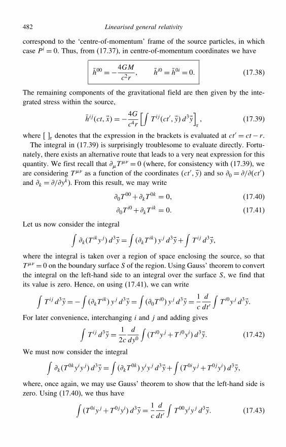
482 Linearised general relativity
correspond to the ‘centre-of-momentum’ frame of the source particles, in whichcase Pi = 0. Thus, from (17.37), in centre-of-momentum coordinates we have
h00 =−4GM
c2r hi0 = h0i = 0 (17.38)
The remaining components of the gravitational field are then given by the inte-grated stress within the source,
hijct x=−4Gc4r
[∫T ijct′ yd3y
]r (17.39)
where r denotes that the expression in the brackets is evaluated at ct′ = ct− r.The integral in (17.39) is surprisingly troublesome to evaluate directly. Fortu-
nately, there exists an alternative route that leads to a very neat expression for thisquantity. We first recall that T
= 0 (where, for consistency with (17.39), weare considering T as a function of the coordinates ct′ y and so 0 = /ct′and k = /yk). From this result, we may write
0T00+ kT
0k = 0 (17.40)
0Ti0+ kT
ik = 0 (17.41)
Let us now consider the integral∫kT
ikyjd3y =∫kT
ik yj d3y+∫T ij d3y
where the integral is taken over a region of space enclosing the source, so thatT = 0 on the boundary surface S of the region. Using Gauss’ theorem to convertthe integral on the left-hand side to an integral over the surface S, we find thatits value is zero. Hence, on using (17.41), we can write∫
T ij d3y =−∫kT
ik yj d3y =∫0T
i0 yj d3y = 1c
d
dt′∫T i0yj d3y
For later convenience, interchanging i and j and adding gives∫T ij d3y = 1
2cd
dy0
∫T i0yj+Tj0yid3y (17.42)
We must now consider the integral∫kT
0kyiyjd3y =∫kT
0k yiyj d3y+∫T 0iy j+T 0jyi d3y
where, once again, we may use Gauss’ theorem to show that the left-hand side iszero. Using (17.40), we thus have∫
T 0iy j+T 0jyi d3y = 1c
d
dt′∫T 00yiyj d3y (17.43)
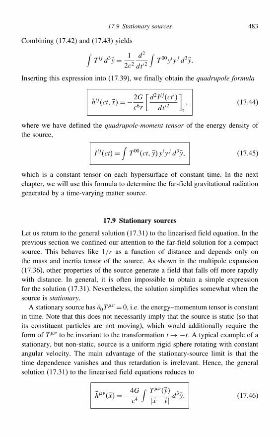
17.9 Stationary sources 483
Combining (17.42) and (17.43) yields∫T ij d3y = 1
2c2d2
dt′2∫T 00yiyj d3y
Inserting this expression into (17.39), we finally obtain the quadrupole formula
hijct x=−2G
c6r
[d2Iijct′
dt′2
]r (17.44)
where we have defined the quadrupole-moment tensor of the energy density ofthe source,
Iijct=∫T 00ct y yiyj d3y (17.45)
which is a constant tensor on each hypersurface of constant time. In the nextchapter, we will use this formula to determine the far-field gravitational radiationgenerated by a time-varying matter source.
17.9 Stationary sources
Let us return to the general solution (17.31) to the linearised field equation. In theprevious section we confined our attention to the far-field solution for a compactsource. This behaves like 1/r as a function of distance and depends only onthe mass and inertia tensor of the source. As shown in the multipole expansion(17.36), other properties of the source generate a field that falls off more rapidlywith distance. In general, it is often impossible to obtain a simple expressionfor the solution (17.31). Nevertheless, the solution simplifies somewhat when thesource is stationary.
A stationary source has 0T = 0, i.e. the energy–momentum tensor is constant
in time. Note that this does not necessarily imply that the source is static (so thatits constituent particles are not moving), which would additionally require theform of T to be invariant to the transformation t→−t. A typical example of astationary, but non-static, source is a uniform rigid sphere rotating with constantangular velocity. The main advantage of the stationary-source limit is that thetime dependence vanishes and thus retardation is irrelevant. Hence, the generalsolution (17.31) to the linearised field equations reduces to
hx=−4Gc4
∫ Tyx−y d
3y (17.46)
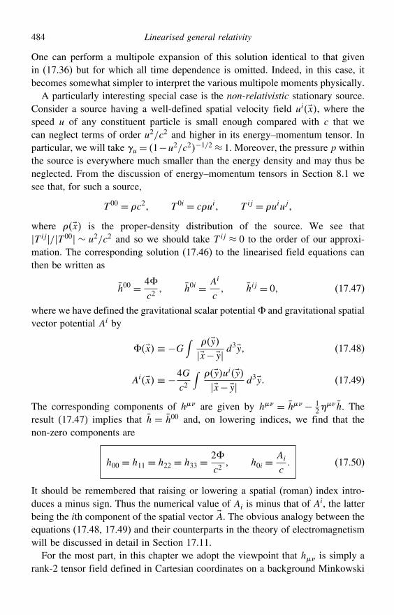
484 Linearised general relativity
One can perform a multipole expansion of this solution identical to that givenin (17.36) but for which all time dependence is omitted. Indeed, in this case, itbecomes somewhat simpler to interpret the various multipole moments physically.
A particularly interesting special case is the non-relativistic stationary source.Consider a source having a well-defined spatial velocity field uix, where thespeed u of any constituent particle is small enough compared with c that wecan neglect terms of order u2/c2 and higher in its energy–momentum tensor. Inparticular, we will take u= 1−u2/c2−1/2 ≈ 1. Moreover, the pressure p withinthe source is everywhere much smaller than the energy density and may thus beneglected. From the discussion of energy–momentum tensors in Section 8.1 wesee that, for such a source,
T 00 = c2 T 0i = cui T ij = uiuj
where x is the proper-density distribution of the source. We see thatT ij/T 00 ∼ u2/c2 and so we should take T ij ≈ 0 to the order of our approxi-mation. The corresponding solution (17.46) to the linearised field equations canthen be written as
h00 = 4%c2
h0i = Ai
c hij = 0 (17.47)
where we have defined the gravitational scalar potential% and gravitational spatialvector potential Ai by
%x ≡ −G∫ yx−y d
3y (17.48)
Aix ≡ −4Gc2
∫ yuiyx−y d3y (17.49)
The corresponding components of h are given by h = h − 12
h. Theresult (17.47) implies that h = h00 and, on lowering indices, we find that thenon-zero components are
h00 = h11 = h22 = h33 =2%c2
h0i =Ai
c (17.50)
It should be remembered that raising or lowering a spatial (roman) index intro-duces a minus sign. Thus the numerical value of Ai is minus that of Ai, the latterbeing the ith component of the spatial vector A. The obvious analogy between theequations (17.48, 17.49) and their counterparts in the theory of electromagnetismwill be discussed in detail in Section 17.11.
For the most part, in this chapter we adopt the viewpoint that h is simply arank-2 tensor field defined in Cartesian coordinates on a background Minkowski
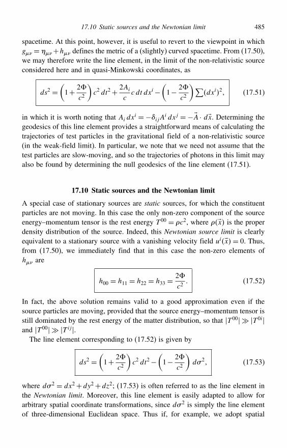
17.10 Static sources and the Newtonian limit 485
spacetime. At this point, however, it is useful to revert to the viewpoint in whichg =+h defines the metric of a (slightly) curved spacetime. From (17.50),we may therefore write the line element, in the limit of the non-relativistic sourceconsidered here and in quasi-Minkowski coordinates, as
ds2 =(1+ 2%
c2
)c2 dt2+ 2Ai
cc dt dxi−
(1− 2%
c2
)∑dxi2 (17.51)
in which it is worth noting that Ai dxi =−ijAi dxj =−A · dx. Determining the
geodesics of this line element provides a straightforward means of calculating thetrajectories of test particles in the gravitational field of a non-relativistic source(in the weak-field limit). In particular, we note that we need not assume that thetest particles are slow-moving, and so the trajectories of photons in this limit mayalso be found by determining the null geodesics of the line element (17.51).
17.10 Static sources and the Newtonian limit
A special case of stationary sources are static sources, for which the constituentparticles are not moving. In this case the only non-zero component of the sourceenergy–momentum tensor is the rest energy T 00 = c2, where x is the properdensity distribution of the source. Indeed, this Newtonian source limit is clearlyequivalent to a stationary source with a vanishing velocity field uix= 0. Thus,from (17.50), we immediately find that in this case the non-zero elements ofh are
h00 = h11 = h22 = h33 =2%c2
(17.52)
In fact, the above solution remains valid to a good approximation even if thesource particles are moving, provided that the source energy–momentum tensor isstill dominated by the rest energy of the matter distribution, so that T 00 T 0iand T 00 T ij.
The line element corresponding to (17.52) is given by
ds2 =(1+ 2%
c2
)c2 dt2−
(1− 2%
c2
)d#2 (17.53)
where d#2 = dx2+dy2+dz2; (17.53) is often referred to as the line element inthe Newtonian limit. Moreover, this line element is easily adapted to allow forarbitrary spatial coordinate transformations, since d#2 is simply the line elementof three-dimensional Euclidean space. Thus if, for example, we adopt spatial
486 Linearised general relativity
spherical polar coordinates then one need only rewrite the spatial line element asd#2 = dr2+ r2 d2+ r2 sin2 d2.It is interesting to compare (17.53) with our discussion of the Newtonian limit
in Chapter 7, where we considered weak gravitational fields, static sources andslowly moving test particles. Under these assumptions, we found that we recoveredthe Newtonian equation of motion for a test particle provided that we made theidentification h00 = 2%/c2, where % is the Newtonian gravitational potential. Inthe solution (17.53), we have arrived at the Newtonian limit without making anyrestriction on the velocity of the test particle. This generalisation is important,as previously we needed to consider only the effects of the g00-component ofthe metric, but, as the above solution shows, the trajectories of relativistic testparticles and photons also depend on the metric spatial components.
As an example of the line element (17.53), let us consider the simple case ofa static spherical object of mass M , so that the Newtonian gravitational potentialis given by % = −GM/r, where r is a radial coordinate. In this case, adoptingspherical polar spatial coordinates, the line element in the Newtonian limit isgiven by
ds2 = c2(1− 2GM
c2r
)dt2−
(1+ 2GM
c2r
)dr2+ r2 d2+ r2 sin2 d2
which is straightforwardly shown to be identical to the Schwarzschild solution,to first order in M . In the Solar System, this approximation is sufficiently accu-rate to determine correctly the bending of light and gravitational redshifts (theShapiro effect) induced by the Sun, giving identical results to those discussed inChapter 10. The accuracy of the above approximation is, however, insufficient topredict perihelion shifts correctly. This is not surprising, since perihelion shift isa cumulative effect.
17.11 The energy–momentum of the gravitational field
Physically, one would expect the gravitational field to carry energy–momentumjust as, for example, the electromagnetic field does. Unfortunately, the task ofassigning an energy density to a gravitational field is famously difficult, bothtechnically and in principle. From our discussion of the equivalence principle inChapter 7, we know that transforming coordinates to a freely falling frame canalways eliminate gravitational effects at any one event. As a result, there is no localnotion of gravitational energy density in general relativity. Moreover, in a generalspacetime there is no reason why energy and momentum should be conserved.In electromagnetism, for example, the conservation of energy and momentumfor the field is a direct consequence of the symmetries of the Minkowski space-time assumed in the theory. In a general spacetime, however, there are no such
17.11 The energy–momentum of the gravitational field 487
symmetries. Even in the linearised gravitational theory developed in this chapter,the field h represents a weak distortion of Minkowski space and so the Lorentzsymmetry properties are lost.
Nevertheless, as we have remarked several times, one can also regard thelinearised theory as describing a simple rank-2 tensor field h in Cartesianinertial coordinates propagating in a fixed Minkowski spacetime background. Wemight therefore hope to assign an energy–momentum tensor to this field just aswe do for electromagnetism, or any other field theory in Minkowski spacetime.As was discussed in Section 17.4, the linearised gravitational theory ignores theenergy–momentum associated with the gravitational field itself (i.e. the ‘gravityof gravity’). To include this contribution, and thereby go beyond the linearisedtheory, one must modify the linearised field equations to read
G1 =−
8Gc4
T+ t
where G1 is the linearised Einstein tensor, T is the energy–momentum tensor
of any matter present and t is the energy–momentum tensor of the gravitationalfield itself. Trivially rearranging this equation gives
G1 +
8Gc4
t =−8Gc4
T
Returning to the exact Einstein equations, however, we may expand beyond firstorder to obtain
G ≡G1 +G2
+· · · = −8Gc4
T (17.54)
where superscripts in parentheses indicate the order of the expansion in h. Thissuggests that, to a good approximation, we should make the identification
t ≡c4
8GG2
(17.55)
This is also in keeping with our experience of other field theories in Minkowskispacetime, such as electromagnetism, in which the energy–momentum tensor isquadratic in the field variable. One should not, however, be too firmly guided bythe analogy with electromagnetism. The reason why the electromagnetic energy–momentum tensor is quadratic in the field variable is that the electromagneticfield (constituted by photons in the quantum description) does not carry chargeand so cannot act as its own source. Indeed, this is the physical reason whyelectromagnetism is a linear theory. In the gravitational case, however, one couldin fact include the higher-order terms in (17.54) in the definition of t; theseterms correspond to the contribution to the total energy–momentum arising fromthe gravitational interaction of the gravitational field with itself. Nevertheless,when the gravitational field is weak these higher-order terms may be neglected.
488 Linearised general relativity
As one might expect from such an heuristic approach, however, there are someshortcomings of the identification (17.55), which we now outline. The terms inthe Einstein tensor that are second-order in h are given by
G2 = R2
− 12R
2− 12hR
1+ 12h
#R1# (17.56)
where R2 denotes the terms in the Ricci tensor that are second-order in h and
R1 and R2 denote the terms in the Ricci scalar that are first- and second-orderin h respectively. Although (17.56), and hence t, is covariant under globalLorentz transformations (although not under general coordinate transformations,as one might expect), it may be may shown, after considerable algebra, thatit is not invariant under the gauge transformation (17.5) (or equivalently theinfinitesimal coordinate transformation (17.4)). One way of circumventing thisproblem is to take seriously the fact that the energy–momentum of a gravitationalfield at a point in spacetime has no real meaning in general relativity, since atany particular event one can always transform to a free-falling frame in whichgravitational effects disappear. This suggests that, at each point in spacetime, oneshould average G2
over a small region in order to probe the physical curvatureof the spacetime, which gives a gauge-invariant measure of the gravitationalfield strength. Denoting this averaging process by · · · , one should thus replace(17.55) by
t ≡c4
8G
⟨G2
⟩ (17.57)
Having made this identification, our task is now an algebraic one of determining
the form of⟨G
2
⟩as a function of h. This is rather a cumbersome calculation,
but the job is made somewhat easier by averaging over small spacetime regions.Since we are averaging over all directions at each point, first derivatives averageto zero. Thus, for any function of position ax, we have a = 0. This has theimportant consequence that ab = ab+ab = 0, and hence wemay swap derivatives in products and inherit only a minus sign, i.e.
ab = −ab (17.58)
Let us begin by considering the last two terms on the right-hand side of (17.56),which depend on the first-order Ricci tensor and Ricci scalar. It will prove mostconvenient to express these in terms of the energy–momentum tensor T of anymatter present. The first-order (linearised) field equation (17.11) can be written as
R1 =−&T− 1
2T
17.11 The energy–momentum of the gravitational field 489
where T ≡ T and &≡ 8G/c4. We also note from this equation that R1 = &T .
Thus, we may write (17.56) as
G2 = R2
− 12R
2− 12&h−h
#T# (17.59)
It therefore remains only to find the form of R2 , from which R2 may
be obtained by contraction. The standard expression for the full Ricci tensoris obtained by contracting (17.7) on its first and last indices. Thus, the termssecond-order in h are given by
R2 =
2## − #
2#+ 1
# 1#
− 1
1## (17.60)
where, on the right-hand side, the superscripts in parentheses denote the order ofexpansion in h for the connection coefficients. The connection coefficients tofirst order were calculated in (17.6), and now including the second-order termswe have
# = 1#
+ 2#+· · ·
= 12h
#+ h
# − #h− 1
2h#h+ h− h+· · ·
Inserting these expressions into (17.60) and simplifying, one finds after a littlealgebra
R2 = − 1
4h#h# + 1
2h##h+ #h− h# − #h
+ 12
#hh#− #h+ 12#h
# − 12
hh+ h− h
(17.61)
Although the third group of terms on the right-hand side is not manifestly symmet-ric in and , this symmetry is easy to verify. In fact, in subsequent calculationsit is convenient to maintain manifest symmetry by writing out this term againwith and reversed and multiplying both terms by one-half.
To evaluate the averaged expression (17.57), we must now calculate⟨R2
⟩.
One first makes use of the result (17.58) to rewrite products of first derivatives in(17.61) in terms of second derivatives. Using the first-order field equation (17.10)to substitute for terms of the form 2h, and then applying (17.58) once more
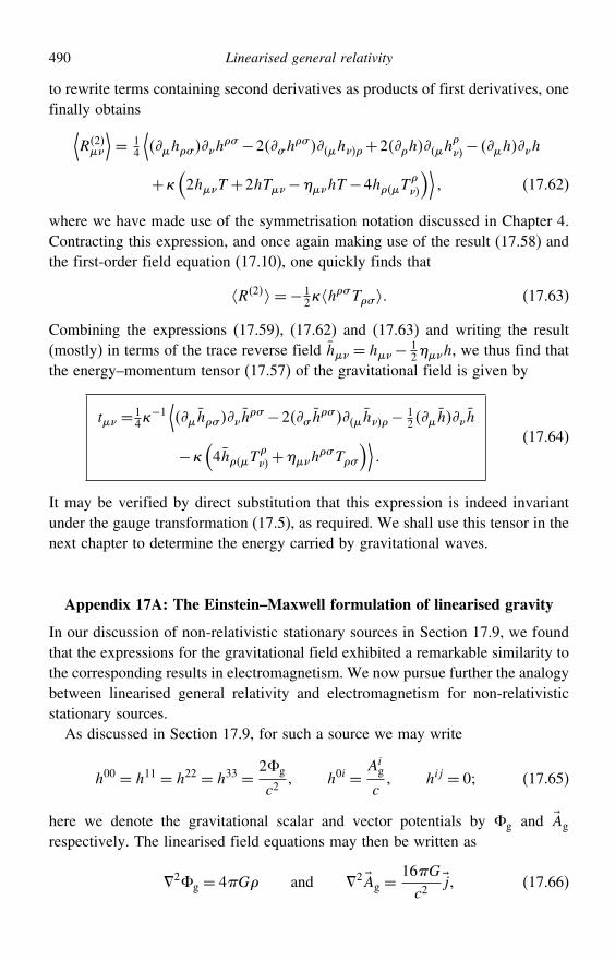
490 Linearised general relativity
to rewrite terms containing second derivatives as products of first derivatives, onefinally obtains⟨
R2
⟩= 1
4
⟨h#h
# −2#h#h+2hh
− hh
+&(2hT +2hT−hT −4hT
)⟩ (17.62)
where we have made use of the symmetrisation notation discussed in Chapter 4.Contracting this expression, and once again making use of the result (17.58) andthe first-order field equation (17.10), one quickly finds that
R2 = − 12&h#T# (17.63)
Combining the expressions (17.59), (17.62) and (17.63) and writing the result(mostly) in terms of the trace reverse field h = h− 1
2h, we thus find thatthe energy–momentum tensor (17.57) of the gravitational field is given by
t = 14&−1⟨h#h
# −2#h#h− 1
2hh
−&(4hT
+h
#T#
)⟩
(17.64)
It may be verified by direct substitution that this expression is indeed invariantunder the gauge transformation (17.5), as required. We shall use this tensor in thenext chapter to determine the energy carried by gravitational waves.
Appendix 17A: The Einstein–Maxwell formulation of linearised gravity
In our discussion of non-relativistic stationary sources in Section 17.9, we foundthat the expressions for the gravitational field exhibited a remarkable similarity tothe corresponding results in electromagnetism. We now pursue further the analogybetween linearised general relativity and electromagnetism for non-relativisticstationary sources.
As discussed in Section 17.9, for such a source we may write
h00 = h11 = h22 = h33 = 2%g
c2 h0i = Ai
g
c hij = 0 (17.65)
here we denote the gravitational scalar and vector potentials by %g and Ag
respectively. The linearised field equations may then be written as
2%g = 4G and 2 Ag =16Gc2
j (17.66)
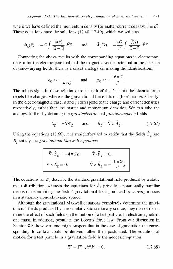
Appendix 17A: The Einstein–Maxwell formulation of linearised gravity 491
where we have defined the momentum density (or matter current density) j ≡ v.These equations have the solutions (17.48, 17.49), which we write as
%gx=−G∫ yx−y d
3y and Agx=−4Gc2
∫ jyx−y d
3y
Comparing the above results with the corresponding equations in electromag-netism for the electric potential and the magnetic vector potential in the absenceof time-varying fields, there is a direct analogy on making the identifications
0↔− 14G
and 0↔−16Gc2
The minus signs in these relations are a result of the fact that the electric forcerepels like charges, whereas the gravitational force attracts (like) masses. Clearly,in the electromagnetic case, and j correspond to the charge and current densitiesrespectively, rather than the matter and momentum densities. We can take theanalogy further by defining the gravitoelectric and gravitomagnetic fields
Eg =−%g and Bg = × Ag (17.67)
Using the equations (17.66), it is straightforward to verify that the fields Eg andBg satisfy the gravitational Maxwell equations
· Eg =−4G · Bg = 0
× Eg = 0 × Bg =−16Gc2
j
The equations for Eg describe the standard gravitational field produced by a static
mass distribution, whereas the equations for Bg provide a notationally familiarmeans of determining the ‘extra’ gravitational field produced by moving massesin a stationary non-relativistic source.
Although the gravitational Maxwell equations completely determine the gravi-tational fields produced by a non-relativistic stationary source, they do not deter-mine the effect of such fields on the motion of a test particle. In electromagnetismone must, in addition, postulate the Lorentz force law. From our discussion inSection 8.8, however, one might suspect that in the case of gravitation the corre-sponding force law could be derived rather than postulated. The equation ofmotion for a test particle in a gravitation field is the geodesic equation
x# + #x
x = 0 (17.68)
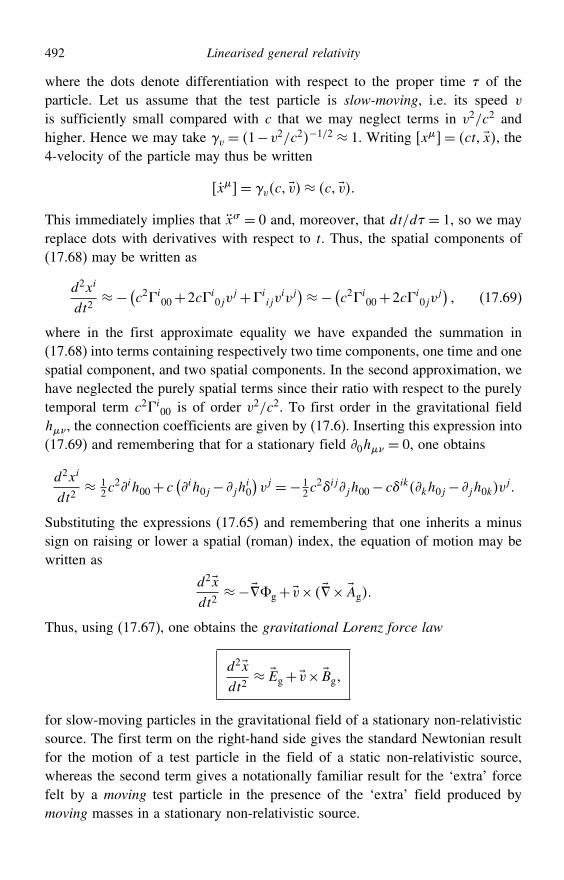
492 Linearised general relativity
where the dots denote differentiation with respect to the proper time of theparticle. Let us assume that the test particle is slow-moving, i.e. its speed v
is sufficiently small compared with c that we may neglect terms in v2/c2 andhigher. Hence we may take v = 1−v2/c2−1/2 ≈ 1. Writing x= ct x, the4-velocity of the particle may thus be written
x= vc v≈ c vThis immediately implies that x# = 0 and, moreover, that dt/d = 1, so we mayreplace dots with derivatives with respect to t. Thus, the spatial components of(17.68) may be written as
d2xi
dt2≈− (c2 i
00+2c i0jv
j+ iijv
ivj)≈− (c2 i
00+2c i0jv
j) (17.69)
where in the first approximate equality we have expanded the summation in(17.68) into terms containing respectively two time components, one time and onespatial component, and two spatial components. In the second approximation, wehave neglected the purely spatial terms since their ratio with respect to the purelytemporal term c2 i
00 is of order v2/c2. To first order in the gravitational fieldh, the connection coefficients are given by (17.6). Inserting this expression into(17.69) and remembering that for a stationary field 0h = 0, one obtains
d2xi
dt2≈ 1
2c2ih00+ c
(ih0j− jh
i0
)vj =− 1
2c2ijjh00− cikkh0j− jh0kv
j
Substituting the expressions (17.65) and remembering that one inherits a minussign on raising or lower a spatial (roman) index, the equation of motion may bewritten as
d2xdt2
≈−%g+v× × Ag
Thus, using (17.67), one obtains the gravitational Lorenz force law
d2xdt2
≈ Eg+v× Bg
for slow-moving particles in the gravitational field of a stationary non-relativisticsource. The first term on the right-hand side gives the standard Newtonian resultfor the motion of a test particle in the field of a static non-relativistic source,whereas the second term gives a notationally familiar result for the ‘extra’ forcefelt by a moving test particle in the presence of the ‘extra’ field produced bymoving masses in a stationary non-relativistic source.
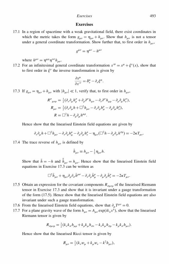
Exercises 493
Exercises
17.1 In a region of spacetime with a weak gravitational field, there exist coordinates inwhich the metric takes the form g = +h. Show that h is not a tensorunder a general coordinate transformation. Show further that, to first order in h,
g = −h
where h = #h# .17.2 For an infinitesimal general coordinate transformation x′ = x+x, show that
to first order in the inverse transformation is given by
x
x′= −
17.3 If g = +h with h 1, verify that, to first order in h,
R# = 1
2 h# +
#h− #h− h
#
R = 12 h+2h− h
− h
R = 2h− h
Hence show that the linearised Einstein field equations are given by
h+2h− h− h
−2h− #h
#=−2&T
17.4 The trace reverse of h is defined by
h ≡ h− 12h
Show that h = −h and ¯h = h. Hence show that the linearised Einstein fieldequations in Exercise 17.3 can be written as
2h+#h# − h
− h
=−2&T
17.5 Obtain an expression for the covariant components R# of the linearised Riemanntensor in Exercise 17.3 and show that it is invariant under a gauge transformationof the form (17.5). Hence show that the linearised Einstein field equations are alsoinvariant under such a gauge transformation.
17.6 From the linearised Einstein field equations, show that T = 0.
17.7 For a plane gravity wave of the form h =A expikx, show that the linearised
Riemann tensor is given by
R# = 12 kk#h+kkh#−kkh#−kk#h
Hence show that the linearised Ricci tensor is given by
R = 12 kw+kw−k2h

494 Linearised general relativity
where k2 = kk and w = kh. Hence show that the linearised Einstein field
equations require that
k2h = kw+kw
17.8 From your answer to Exercise 17.7, show that for k2 = 0 one requires R# = 0.Hence show that this case does not correspond to a physical wave but merely aperiodic oscillation of the coordinate system.
17.9 From your answer to Exercise 17.7, show that for k2 = 0 one requires kh = 0.Hence show that the wavevector k is an eigenvector of the Riemann tensor in thesense that R#k
= 0.17.10 Show explicitly that
hx#= h0x
#−2&∫Gx# −y#Ty#d4y
is a solution of the linearised Einstein field equations in the Lorenz gauge ifh0x
# is any solution of the linearised field equations in vacuo and Gx# −y#
satisfies
2xGx# −y#= 4x# −y#
17.11 The Green’s function Gx# −y# satisfies the equation
2xGx# −y#= 4x# −y#
Show that the four-dimensional Dirac delta function can be written as
4x# −y#= 124
∫exp
[ik(x−y
)]d4k
Hence, by writing the Green’s function in terms of its Fourier transform Gk#,show that
Gx# −y#=− 124
∫ 1k2
exp[ik(x−y
)]d4k
where k2 = kk.
17.12 Verify that the solution in Exercise 17.10 satisfies the Lorenz gauge condition.17.13 Prove the results (17.32, 17.33) for the derivatives of a function of retarded time.17.14 By writing r ≡ x = ijx
ixj−1/2, show that
i
(1r
)=−xi
r
Hence show that
ij
(1r
)= 3xixj− r2ij
r5
Exercises 495
17.15 In Newtonian gravity, the gravitational potential %x produced by some densitydistribution x is given by
%x=−G∫V
yx−y d
3y
where the integral extends over the volume of the distribution. Show that
1
x−y =1
x +x · yx3 +
(1
x3)
Hence show that the gravitational potential can be written as
%x=−GM
x −G d · xx3 +
(1
x3)
where
M =∫Vyd3y and d =
∫Vyy d3y
17.16 From the conservation equation T = 0, show that
0T00+ kT
0k = 0 and 0Ti0+ kT
ik = 0
By integrating each equation over a spatial volume V whose bounding surface S
encloses the energy–momentum source and using the three-dimensional divergencetheorem, show that the quantities
Mc2 ≡∫VT 00 d3y and Pi ≡
∫T i0 d3y
are constants and give a physical interpretation of them.17.17 For a stationary source, show that 0T
0i = 0. Hence show that∫VT 0iy j+T 0jyi d3y = 0
where the spatial volume V encloses the source.17.18 For a non-relativistic stationary source, show that, in centre-of-momentum
coordinates,
h00x = −4GM
c2x +
(1
x2)
h0ix = 2G
c3x3 xjJij+
(1
x3)
hijx = 0
where the quantities M and J ij are given by
M =∫Vyd3y and J ij =
∫V
[yipjy−y jpiy] d3y
496 Linearised general relativity
in which y is the proper density distribution of the source and piy= yuiyis the momentum density distribution of the source. Give a physical interpretationof J ij .Hint: You will find your answer to Exercise 17.17 useful.
17.19 Use your answer to Exercise 17.18 to show that, for a stationary non-relativisticsource, the gravitational scalar and vector potentials respectively are given toleading order in 1/x by
%gx=−GM
x and Agx=−2G
c2x3 J ×x
where J = ∫y× pd3y is the total angular momentum vector of the source.
Show further that these expressions are exact in the linear theory for a sphericallysymmetric source.
17.20 Use your answer to Exercise 17.19 to show that, in the linear theory, the lineelement outside a spherically symmetric matter distribution rotating about thez-axis at a steady rate is given by
ds2= c2(1− 2GM
c2r
)dt2+ 4GJ
c2r3xdy−y dxdt−
(1+ 2GM
c2r
)dx2+dy2+dz2
where r = x. Show that this is equal to the Kerr line element to first order in M
and J .Hint: Ai dx
i =−ijAj dxi =−A ·dx and J ×x ·dx = J · x×dx.17.21 If g = +h, show that the terms in the Einstein tensor that are second order
in h are given by
G2 = R2
− 12R
2− 12hR
1+ 12h
#R1#
where R2 denotes the terms in the Ricci tensor that are second order in h, and
R1 and R2 denote the terms in the Ricci scalar that are first and second orderin h respectively. Show further that this quantity is not invariant under a gaugetransformation of the form (17.5).
17.22 Verify that the energy–momentum tensor of the linearised gravitational field isgiven by (17.64). Show further that this tensor is invariant under a gauge trans-formation of the form (17.5).
17.23 Use your answer to Exercise 17.19 to show that, in the linear theory, a sphericallysymmetric body of mass M rotating steadily with angular momentum J producesgravitoelectric and gravitomagnetic fields given respectively by
Egx=−GM
x2 x and Bgx=2G
c2x3[J −3
(J · x) x] where x is a unit vector in the x- direction.Hint: For any scalar field and spatial vector fields a and b one has a=×a+×a and ×a×b= a · b−b · a+b · a−a · b. Also,1/x3=−3x/x5.
Exercises 497
17.24 Consider a particle moving under gravity at speed v in a circular orbit of radiusr in the equatorial plane of the body in Exercise 17.23. Show that the vectoracceleration of the particle is given by
a=−GM
r2r± 2GJv
c2r3r
where r is the position vector of the orbiting particle and the plus and minus signscorresponding to prograde and retrograde orbits respectively. Hence show that theangular velocity of the particle is given to first order in J by
2 = GM
r3∓ 2GJ
c2r4
√GM
r
where the minus and plus signs now correspond to prograde and retrograde orbitsrespectively. Thus show that the retrograde orbit has a shorter period than theprograde orbit.
17.25 In electromagnetism, the magnetic dipole moment of a current density distributionjy is defined by m = 1
2
∫y×jd3y, and the force and torque on the dipole
in a magnetic field B are given by F = m · B and T = m× B respectively.Hence deduce that, in linearised gravity, the force and torque exerted by thegravitomagnetic field Bg on a spinning body with spin angular momentum s aregiven respectively by
Fg = 12 s · Bg and Tg = 1
2 s× Bg
Thus show that the spin angular momentum of the body will evolve as
dsdt= 1
2 s× Bg
and therefore that s precesses about Bg with angular velocity =− 12 Bg (i.e. in
the negative sense). This is called the Lens–Thirring precession.17.26 A gyroscope is in orbit about the massive rotating body in Exercise 17.23. Use
your answer to Exercise 17.25 to show that the precessional angular velocity vectorof the gyroscope is given by
= G
c2x3[3J · x x− J
]
where x is the position vector of the gyroscope relative to the centre of the massivebody. Show that this result agrees with that derived in Section 13.20 when x pointsalong J .
18
Gravitational waves
In the previous chapter, we saw that the linearised field equations of generalrelativity could be written in the form of a wave equation
2h =−2&T (18.1)
provided that the h satisfy the Lorenz gauge condition
h = 0 (18.2)
This suggests the existence of gravitational waves in an analogous manner to thatin which Maxwell’s equations predict electromagnetic waves. In this chapter, wediscuss in detail the propagation, generation and detection of such gravitationalradiation. As in the previous chapter, we will adopt the viewpoint that h issimply a symmetric tensor field (under global Lorentz transformations) definedon a flat Minkowski background spacetime.
18.1 Plane gravitational waves and polarisation states
In Section 17.5, we showed that the general solution of the linearised fieldequations in vacuo may be written as the superposition of plane-wave solutionsof the form
h = A expikx (18.3)
where the A are constant (and, in general, complex) components of a symmetrictensor and k are the constant (real) components of a vector. The Lorenz gaugecondition is satisfied provided that the additional constraint
Ak = 0 (18.4)
498
18.1 Plane gravitational waves and polarisation states 499
is obeyed. Physical solutions corresponding to propagating plane gravitationalwaves in empty space may be obtained by taking the real part of (18.3):
h = A expikx
= 12A
expikx+ 1
2A∗ exp−ikx
which is clearly just a superposition of two plane waves of the form (18.3).The constants A are the components of the amplitude tensor, and the k ≡
k are the components of the 4-wavevector. It is conventional to denotethe components of the 4-wavevector by k = /c k, where k is the spatial3-wavevector in the direction of propagation and is the angular frequency ofthe wave. The nullity of k implies that 2 = c2k2, and so both the group andphase velocity of a gravitational wave are equal to the speed of light.
Since A =A, the amplitude tensor has 10 different (complex) components,but the four Lorenz gauge conditions (18.4) reduce the number of independentcomponents to six. Moreover, we still have the freedom to make a further gaugetransformation of the form (17.5), which will preserve the Lorenz gauge providedthat we choose the four functions x so that they satisfy 2= 0. As we showbelow, this may be used to reduce the number of independent components in theamplitude matrix from six to just two. This results in two possible polarisationsfor plane gravitational waves.
It is convenient to consider the concrete example of a plane gravitationalwave propagating in the x3-direction, in which case the components of the 4-wavevector are
k= k00 k (18.5)
where k = /c. The Lorenz gauge condition (18.4) then immediately givesA3 = A0. Together with the symmetry of the amplitude tensor, this impliesthat all the components A can be expressed in terms of the six quantitiesA00A01A02A11A12A22:
A=
⎛⎜⎜⎜⎝A00 A01 A02 A00
A01 A11 A12 A01
A02 A12 A22 A02
A00 A01 A02 A00
⎞⎟⎟⎟⎠
We may now perform a gauge transformation of the form (17.5) to simplify theamplitude tensor still further. To preserve the Lorenz gauge condition we mustensure that 2 = 0. A suitable transformation, which satisfies this condition, isgiven by
= expikx
500 Gravitational waves
where the are constants. Substituting this expression into the transformationlaw (17.12) for the trace reverse tensor h, which we assume to be of the form(18.3), one quickly finds that the amplitude tensor transforms as
A′ = A− ik− ik+ ik (18.6)
Using the expression (18.5) for the 4-wavevector and the result (18.6), we obtain
A′00 = A00− ik0+ 3 A′11 = A11− ik0− 3
A′01 = A01− ik1 A′12 = A12
A′02 = A02− ik2 A′22 = A22− ik0− 3
Now, by choosing the constants as follows,
0 =−i2A00+A11+A22/4k 1 =−iA01/k
2 =−iA02/k 3 =−i2A00−A11−A22/4k
we obtain
A′00 = A′01 = A′02 = 0 and A′11 =−A′22On dropping primes, the first condition means that only A11A12 and A22 are
non-zero. Moreover, the second condition means that only two of these can bespecified independently. Choosing A11 ≡ a and A12 ≡ b as the two independent(in general, complex) components in our new gauge, we thus have
ATT=
⎛⎜⎜⎜⎝0 0 0 00 a b 00 b −a 00 0 0 0
⎞⎟⎟⎟⎠ (18.7)
for a wave travelling in the x3-direction. As indicated, the new gauge we haveadopted is known as the transverse-traceless gauge (or TT gauge), which we willdiscuss in more detail in Section 18.3. For now we simply note that (18.7) implieshTT = 0= hTT (hence the term traceless) and h
TT = h
TT for our plane wave.
It is also convenient to introduce the two linear polarisation tensors e1 ande2 , the components of which are obtained by setting a= 1 b= 0 and a= 0 b= 1respectively in (18.7). The general amplitude tensor in the TT gauge for a wavetravelling in the x3-direction can then be written as
ATT = ae
1 +be
2
It follows that all possible polarisations of the gravitational wave may be obtainedby superposing just two polarisations, with arbitrary amplitudes and relativephases.
18.2 Analogy between gravitational and electromagnetic waves 501
18.2 Analogy between gravitational and electromagnetic waves
Before going on to discuss gravitational waves in more detail, it is instructive toillustrate the close analogy with electromagnetic waves. By adopting the Lorenzgauge condition A
= 0, the electromagnetic field equations in free space takethe form 2A = 0. These admit plane-wave solutions of the form
A = Q expikx
where the Q are the constant components of the amplitude vector. The fieldequations again imply that the 4-wavevector k is null and the Lorenz gaugecondition requires that Qk = 0, thereby reducing the number of independentcomponents in the amplitude vector to three. In particular, if we again considera wave propagating in the x3-direction then k = k00 k and the Lorenzgauge condition implies that Q0 =Q3, so that
Q= Q0Q1Q2Q0
The Lorenz gauge condition is preserved by any further gauge transformationof the form A → A+ , provided that 2 = 0. An appropriate gaugetransformation that satisfies this condition is
= expikx
where is a constant. This yields Q′ =Q+ ik, and so
Q′0 =Q0+ ik Q′1 =Q1 Q′2 =Q2
By choosing = −iQ0/k, on dropping primes we have Q0 = 0. In the newgauge, the amplitude vector has just two independent components, Q1 and Q2,and the electromagnetic fields are transverse to the direction of propagation. Byintroducing the two linear polarisation vectors
e1 = 0100 and e
2 = 0010
we may write the general amplitude vector as
Q = ae1 +be
2
where a and b are arbitrary (in general, complex) constants.If b= 0 then as the electromagnetic wave passes a free positive test charge this
will oscillate in the x1-direction with a magnitude that varies sinusoidally withtime. Similarly, if a= 0 then the test charge will oscillate in the x2-direction. Theparticular combinations of linear polarisations given by b = ±ia give circularlypolarised waves, in which the mutually orthogonal linear oscillations combine insuch a way that the test charge moves in a circle.
502 Gravitational waves
18.3 Transforming to the transverse-traceless gauge
In Section 18.1, we considered only the transformation into the TT gauge of aplane gravitational wave travelling in the x3-direction. We now consider a generalgravitational perturbation h satisfying the empty-space linearised field equationand the Lorenz gauge condition. As discussed previously, a gauge transformationof the form (17.5) will preserve the Lorenz gauge condition provided that the fourfunctions x satisfy 2 = 0. From (17.12), the trace-reverse field tensortransforms as
h′ = h− − +##
Since the components h also satisfy the in vacuo wave equation 2h = 0,this gauge transformation may be used to set any four linear combinations of theh′ to zero. The TT gauge is defined by choosing
h0iTT ≡ 0 and hTT ≡ 0 (18.8)
This last condition means that hTT = hTT, and these quantities may therefore
be used interchangeably. Moreover, setting = 0 and = j respectively in theLorenz gauge condition h
TT = 0, and using (18.8), gives the constraints
0h00TT = 0 and ih
ijTT = 0 (18.9)
We note that, if the gravitational field perturbation is non-stationary (i.e. it dependson t), as for a general gravitational wave disturbance, the first constraint in (18.9)implies that h00TT also vanishes and so h
0TT = 0 for all . In other words, in this
case only the spatial components hijTT are non-zero.Let us now consider the particular case of an arbitrary plane gravitational wave
of the form (18.3) and satisfying the Lorenz gauge condition. The conditions(18.4) immediately imply that
A0iTT = 0 and ATT
= 0
Moreover, the conditions (18.9) also require that
A00TT = 0 and A
ijTTkj = 0
These last conditions ensure that, quite generally, a plane gravitational wave istransverse, like electromagnetic waves.
The above conditions tell us the constraints on the form of ATT. We must
now consider how to construct this tensor for a plane wave with a given spatialwavevector k and amplitude matrix A. First, it is clear that we need consider
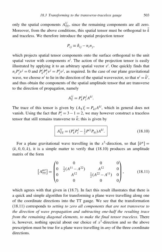
18.3 Transforming to the transverse-traceless gauge 503
only the spatial components AijTT, since the remaining components are all zero.
Moreover, from the above conditions, this spatial tensor must be orthogonal to kand traceless. We therefore introduce the spatial projection tensor
Pij ≡ ij−ninj
which projects spatial tensor components onto the surface orthogonal to the unitspatial vector with components ni. The action of the projection tensor is easilyillustrated by applying it to an arbitrary spatial vector vi. One quickly finds thatniP
ijv
j = 0 and PikP
kj v
j = Pijv
j , as required. In the case of our plane gravitational
wave, we choose ni to lie in the direction of the spatial wavevector, so that ni= ki,and thus obtain the components of the spatial amplitude tensor that are transverseto the direction of propagation, namely
AijT = Pi
kPjl A
kl
The trace of this tensor is given by ATii = PklA
kl, which in general does notvanish. Using the fact that Pi
i = 3−1= 2, we may however construct a traceless
tensor that still remains transverse to k; this is given by
AijTT = Pi
kPjl − 1
2PijPklA
kl (18.10)
For a plane gravitational wave travelling in the x3-direction, so that k =k00 k, it is a simple matter to verify that (18.10) produces an amplitudematrix of the form
[ATT
]=⎛⎜⎜⎜⎝0 0 0 00 1
2A11−A22 A12 0
0 A12 12A
22−A11 00 0 0 0
⎞⎟⎟⎟⎠ (18.11)
which agrees with that given in (18.7). In fact this result illustrates that there isa quick and simple algorithm for transforming a plane wave travelling along oneof the coordinate directions into the TT gauge. We see that the transformation(18.11) corresponds to setting to zero all components that are not transverse tothe direction of wave propagation and subtracting one-half the resulting tracefrom the remaining diagonal elements, to make the final tensor traceless. Thereis, however, nothing special about our choice of x3-direction and so the aboveprescription must be true for a plane wave travelling in any of the three coordinatedirections.

504 Gravitational waves
18.4 The effect of a gravitational wave on free particles
Let us now consider the motion of a set of test particles, initially at rest, in thepresence of a gravitational wave. In fact, in the latter case it is not enough toconsider the trajectory of just a single test particle, as we discuss below. To obtaina coordinate-independent measure of the effects of the wave, it is necessary toconsider the relative motion of a set of nearby particles.
First consider a single free test particle, whose 4-velocity u# must satisfy thegeodesic equation
du#
d+ #
uu = 0
Suppose that the particle is initially at rest in our chosen coordinate system, sothat u= c1000. The geodesic equation then reads
du#
d=−c2 #
00 =− 12c
2#0h0+ 0h0− h00
where in the last equality we have used (17.6) to obtain the connection coefficientsto first order in terms of the derivatives of h. Let us now adopt the TT gauge,which we may do for any general gravitational wave disturbance in vacuo. Fromthe discussion in Section 18.3, we know that hTT0 = 0 for all values of . Thus,initially, du#/d = 0 and so the particle will still be at rest a moment later.The argument may then be repeated, showing that the particle remains at restforever, regardless of the passing of the gravitational wave. In other words u#=c1000 is a solution of the geodesic equation in this case, as may readily beverified by direct substitution.
What has gone wrong here? The key point is that ‘at rest’ in this context meanssimply that the particle has constant spatial coordinates. What we have uncoveredis that by choosing the TT gauge we have found a coordinate system that staysattached to individual particles. This has no coordinate-invariant physical meaning.To obtain a proper physical interpretation of the effect of a passing gravitationalwave, we must consider a set of nearby particles.
Let us therefore consider a cloud of non-interacting free test particles. Fromthe above discussion, the worldlines of the particles are curves having constantspatial coordinates. Thus the small spacelike vector = 0 1 2 3 givingthe coordinate separation between any two nearby particles is constant (this mayalso be shown explicitly by demonstrating that the equation of geodesic deviation(7.24) has = constant as a solution in this case). Although the coordinateseparation of the particles is constant, this does not mean that their physical spatialseparation l is constant. The latter is given by
l2 =−gijij = ij−hijij
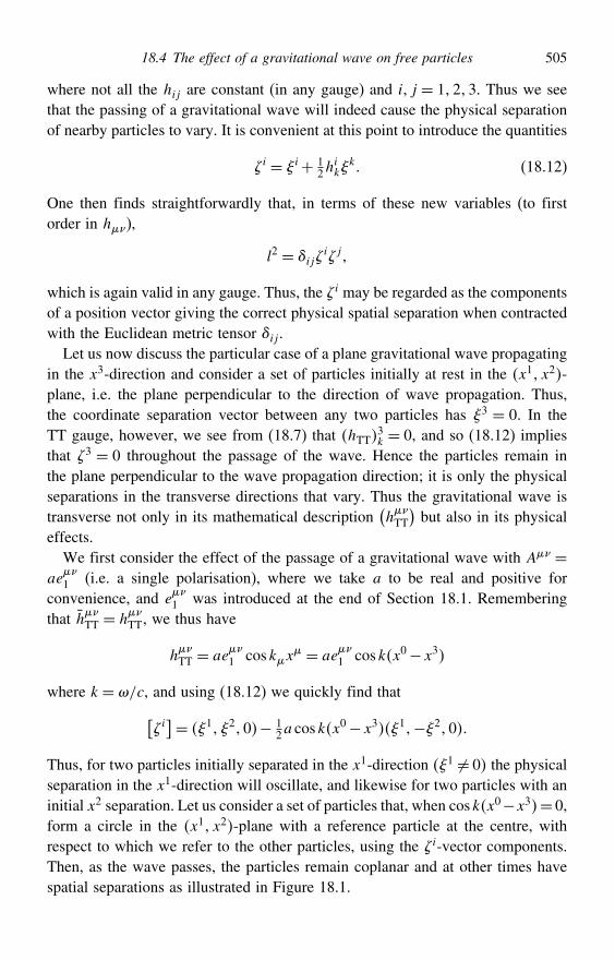
18.4 The effect of a gravitational wave on free particles 505
where not all the hij are constant (in any gauge) and i j = 123. Thus we seethat the passing of a gravitational wave will indeed cause the physical separationof nearby particles to vary. It is convenient at this point to introduce the quantities
i = i+ 12h
ik
k (18.12)
One then finds straightforwardly that, in terms of these new variables (to firstorder in h),
l2 = ijij
which is again valid in any gauge. Thus, the i may be regarded as the componentsof a position vector giving the correct physical spatial separation when contractedwith the Euclidean metric tensor ij .Let us now discuss the particular case of a plane gravitational wave propagating
in the x3-direction and consider a set of particles initially at rest in the x1 x2-plane, i.e. the plane perpendicular to the direction of wave propagation. Thus,the coordinate separation vector between any two particles has 3 = 0. In theTT gauge, however, we see from (18.7) that hTT
3k = 0, and so (18.12) implies
that 3 = 0 throughout the passage of the wave. Hence the particles remain inthe plane perpendicular to the wave propagation direction; it is only the physicalseparations in the transverse directions that vary. Thus the gravitational wave istransverse not only in its mathematical description
(hTT
)but also in its physical
effects.We first consider the effect of the passage of a gravitational wave with A =
ae1 (i.e. a single polarisation), where we take a to be real and positive for
convenience, and e1 was introduced at the end of Section 18.1. Remembering
that hTT = hTT, we thus have
hTT = ae
1 coskx
= ae1 coskx0−x3
where k= /c, and using (18.12) we quickly find that[i]= 1 20− 1
2a coskx0−x31−20
Thus, for two particles initially separated in the x1-direction 1 = 0 the physicalseparation in the x1-direction will oscillate, and likewise for two particles with aninitial x2 separation. Let us consider a set of particles that, when coskx0−x3= 0,form a circle in the x1 x2-plane with a reference particle at the centre, withrespect to which we refer to the other particles, using the i-vector components.Then, as the wave passes, the particles remain coplanar and at other times havespatial separations as illustrated in Figure 18.1.
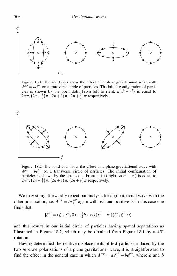
506 Gravitational waves
ζ 1
ζ 2
Figure 18.1 The solid dots show the effect of a plane gravitational wave withA = ae
1 on a transverse circle of particles. The initial configuration of parti-
cles is shown by the open dots. From left to right, kx0 − x3 is equal to2n
(2n+ 1
2
) 2n+1
(2n+ 3
2
) respectively.
ζ1
ζ 2
Figure 18.2 The solid dots show the effect of a plane gravitational wave withA = be
2 on a transverse circle of particles. The initial configuration of
particles is shown by the open dots. From left to right, kx0− x3 is equal to2n
(2n+ 1
2
) 2n+1
(2n+ 3
2
) respectively.
We may straightforwardly repeat our analysis for a gravitational wave with theother polarisation, i.e. A = be
2 again with real and positive b. In this case one
finds that
i= 1 20− 12b coskx
0−x32 10
and this results in our initial circle of particles having spatial separations asillustrated in Figure 18.2, which may be obtained from Figure 18.1 by a 45rotation.
Having determined the relative displacements of test particles induced by thetwo separate polarisations of a plane gravitational wave, it is straightforward tofind the effect in the general case in which A = ae
1 + be
1 , where a and b
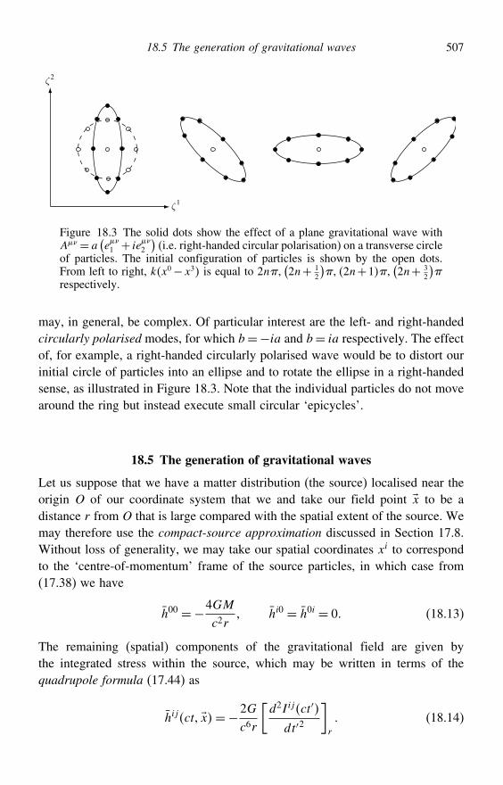
18.5 The generation of gravitational waves 507
ζ 1
ζ 2
Figure 18.3 The solid dots show the effect of a plane gravitational wave withA = a
(e1 + ie
2
)(i.e. right-handed circular polarisation) on a transverse circle
of particles. The initial configuration of particles is shown by the open dots.From left to right, kx0−x3 is equal to 2n
(2n+ 1
2
) 2n+1
(2n+ 3
2
)
respectively.
may, in general, be complex. Of particular interest are the left- and right-handedcircularly polarised modes, for which b=−ia and b= ia respectively. The effectof, for example, a right-handed circularly polarised wave would be to distort ourinitial circle of particles into an ellipse and to rotate the ellipse in a right-handedsense, as illustrated in Figure 18.3. Note that the individual particles do not movearound the ring but instead execute small circular ‘epicycles’.
18.5 The generation of gravitational waves
Let us suppose that we have a matter distribution (the source) localised near theorigin O of our coordinate system that we and take our field point x to be adistance r from O that is large compared with the spatial extent of the source. Wemay therefore use the compact-source approximation discussed in Section 17.8.Without loss of generality, we may take our spatial coordinates xi to correspondto the ‘centre-of-momentum’ frame of the source particles, in which case from(17.38) we have
h00 =−4GM
c2r hi0 = h0i = 0 (18.13)
The remaining (spatial) components of the gravitational field are given bythe integrated stress within the source, which may be written in terms of thequadrupole formula (17.44) as
hijct x=−2G
c6r
[d2Iijct′
dt′2
]r
(18.14)
508 Gravitational waves
In this expression r denotes that the expression in the brackets is evaluated atthe retarded time ct′ = ct− r, and the quadrupole-moment tensor of the source is
Iijct=∫T 00ct yyiyj d3y (18.15)
Thus, we see that, in the compact-source approximation, the far field of the sourcefalls into two parts: a steady field (18.13) from the total constant ‘mass’ M of thesource and a possibly varying field (18.14) arising from the integrated internalstresses of the source. It is clearly the latter that will be responsible for any emittedgravitational radiation.
For slowly moving source particles we have T 00 ≈ c2, where is the properdensity of the source, and so the integral (18.15) may be written as
Iijct= c2∫ct xxixj d3x (18.16)
Thus, the gravitational wave produced by an isolated non-relativistic source isproportional to the second derivative of the quadrupole moment of the matter-density distribution. By contrast, the leading contribution to electromagnetic radi-ation is the first derivative of the dipole moment of the charge density distribution.This fundamental difference between the two theories may be easily understoodfrom elementary considerations. Using to denote either the proper mass densityor the proper charge density, the volume integral
∫dV over the source is constant
in time for both electromagnetism and linearised gravitation and so generates noradiation. Now consider the next moment
∫xi dV , i.e. the dipole moment. For
electromagnetism, this gives the position of the centre of charge of the source,which can move with time and hence have a non-zero time derivative; thisprovides the dominant contribution in the generation of electromagnetic radiation.For gravitation, however,
∫xi dV gives the centre of mass of the source and,
for an isolated system, conservation of momentum means that it cannot changewith time and so cannot contribute to the generation of gravitational waves. Thus,it is the generally much smaller quadrupole moment, which measures the shapeof the source, that is dominant in generating gravitational waves. This fact, andthe weak coupling of gravitation to matter, means that gravitational radiationis much weaker than electromagnetic radiation. As a corollary, we note that aspherically symmetric system has a zero quadrupole moment and thus cannot emitgravitational radiation.
As an illustration of the generation of gravitational waves, let us consider twoparticles A and B of equal mass M moving (non-relativistically) in circular orbitsof radius a about their common centre of mass with an angular speed (seeFigure 18.4). This might represent a simple model of a binary star system, in
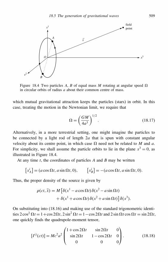
18.5 The generation of gravitational waves 509
x
x1
x2
x3
B
A
O
fieldpoint
Figure 18.4 Two particles A, B of equal mass M rotating at angular speed in circular orbits of radius a about their common centre of mass.
which mutual gravitational attraction keeps the particles (stars) in orbit. In thiscase, treating the motion in the Newtonian limit, we require that
=(GM
4a3
)1/2
(18.17)
Alternatively, in a more terrestrial setting, one might imagine the particles tobe connected by a light rod of length 2a that is spun with constant angularvelocity about its centre point, in which case need not be related to M and a.For simplicity, we shall assume the particle orbits to lie in the plane x3 = 0, asillustrated in Figure 18.4.
At any time t, the coordinates of particles A and B may be written[xiA]= a costa sint0
[xiB]=−a costa sint0
Thus, the proper density of the source is given by
ct x = M[x1−a costx2−a sint
+ x1+a costx2+a sint]x3
On substituting into (18.16) and making use of the standard trigonometric identi-ties 2 cos2t= 1+cos2t2 sin2t= 1−cos2t and 2 sint cost = sin 2t,one quickly finds the quadrupole-moment tensor,
Iijct=Mc2a2
⎛⎜⎝1+ cos2t sin 2t 0sin 2t 1− cos2t 0
0 0 0
⎞⎟⎠ (18.18)
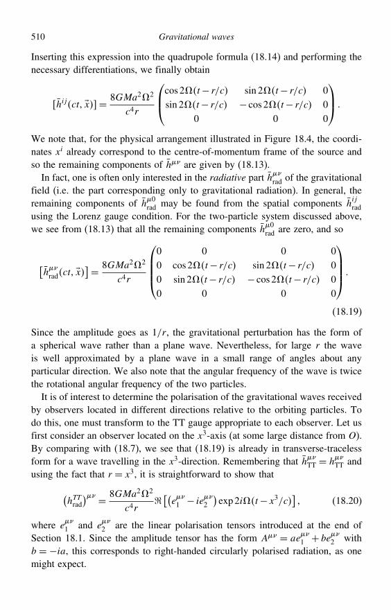
510 Gravitational waves
Inserting this expression into the quadrupole formula (18.14) and performing thenecessary differentiations, we finally obtain
hijct x= 8GMa22
c4r
⎛⎜⎝cos2t− r/c sin 2t− r/c 0sin 2t− r/c − cos2t− r/c 0
0 0 0
⎞⎟⎠
We note that, for the physical arrangement illustrated in Figure 18.4, the coordi-nates xi already correspond to the centre-of-momentum frame of the source andso the remaining components of h are given by (18.13).In fact, one is often only interested in the radiative part hrad of the gravitational
field (i.e. the part corresponding only to gravitational radiation). In general, theremaining components of h0rad may be found from the spatial components h
ijrad
using the Lorenz gauge condition. For the two-particle system discussed above,we see from (18.13) that all the remaining components h0rad are zero, and so
[hradct x
]= 8GMa22
c4r
⎛⎜⎜⎜⎝0 0 0 00 cos2t− r/c sin 2t− r/c 00 sin 2t− r/c − cos2t− r/c 00 0 0 0
⎞⎟⎟⎟⎠
(18.19)
Since the amplitude goes as 1/r, the gravitational perturbation has the form ofa spherical wave rather than a plane wave. Nevertheless, for large r the waveis well approximated by a plane wave in a small range of angles about anyparticular direction. We also note that the angular frequency of the wave is twicethe rotational angular frequency of the two particles.
It is of interest to determine the polarisation of the gravitational waves receivedby observers located in different directions relative to the orbiting particles. Todo this, one must transform to the TT gauge appropriate to each observer. Let usfirst consider an observer located on the x3-axis (at some large distance from O).By comparing with (18.7), we see that (18.19) is already in transverse-tracelessform for a wave travelling in the x3-direction. Remembering that hTT = h
TT and
using the fact that r = x3, it is straightforward to show that(hTTrad
) = 8GMa22
c4r [(e1 − ie
2
)exp2it−x3/c
] (18.20)
where e1 and e
2 are the linear polarisation tensors introduced at the end of
Section 18.1. Since the amplitude tensor has the form A = ae1 + be
2 with
b = −ia, this corresponds to right-handed circularly polarised radiation, as onemight expect.
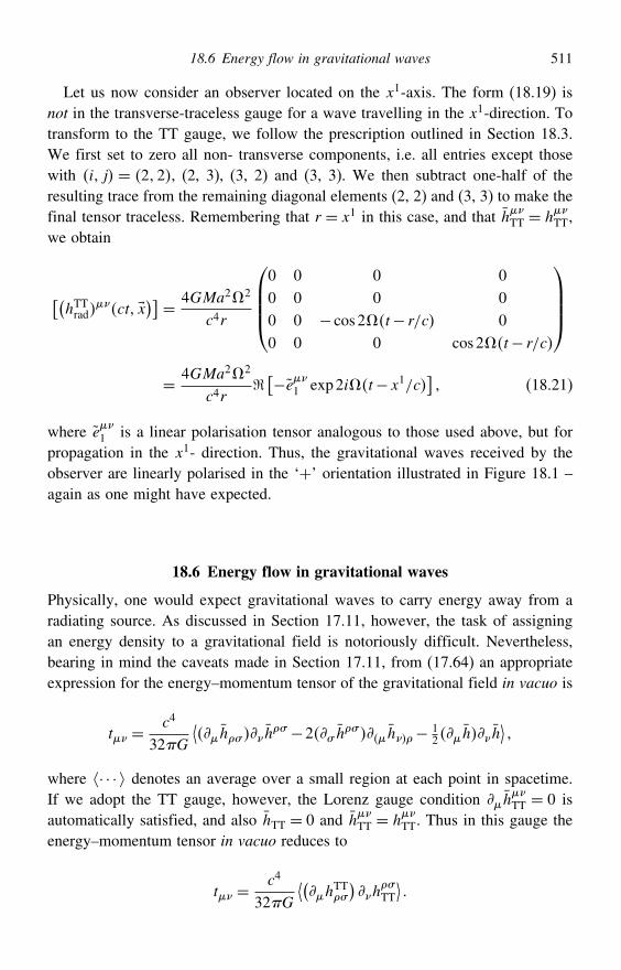
18.6 Energy flow in gravitational waves 511
Let us now consider an observer located on the x1-axis. The form (18.19) isnot in the transverse-traceless gauge for a wave travelling in the x1-direction. Totransform to the TT gauge, we follow the prescription outlined in Section 18.3.We first set to zero all non- transverse components, i.e. all entries except thosewith i j = 22, (2, 3), (3, 2) and (3, 3). We then subtract one-half of theresulting trace from the remaining diagonal elements (2, 2) and (3, 3) to make thefinal tensor traceless. Remembering that r = x1 in this case, and that hTT = h
TT,
we obtain
[(hTTrad
ct x)] = 4GMa22
c4r
⎛⎜⎜⎜⎝0 0 0 00 0 0 00 0 − cos2t− r/c 00 0 0 cos2t− r/c
⎞⎟⎟⎟⎠= 4GMa22
c4r [−e1 exp2it−x1/c
] (18.21)
where e1 is a linear polarisation tensor analogous to those used above, but for
propagation in the x1- direction. Thus, the gravitational waves received by theobserver are linearly polarised in the ‘+’ orientation illustrated in Figure 18.1 –again as one might have expected.
18.6 Energy flow in gravitational waves
Physically, one would expect gravitational waves to carry energy away from aradiating source. As discussed in Section 17.11, however, the task of assigningan energy density to a gravitational field is notoriously difficult. Nevertheless,bearing in mind the caveats made in Section 17.11, from (17.64) an appropriateexpression for the energy–momentum tensor of the gravitational field in vacuo is
t =c4
32G
⟨h#h
# −2#h#h− 1
2hh⟩
where · · · denotes an average over a small region at each point in spacetime.If we adopt the TT gauge, however, the Lorenz gauge condition h
TT = 0 is
automatically satisfied, and also hTT = 0 and hTT = h
TT. Thus in this gauge the
energy–momentum tensor in vacuo reduces to
t =c4
32G
⟨(h
TT#
)h
#TT
⟩
512 Gravitational waves
We will assume further that we are considering only the radiative part of thegravitational field, in which case we know from the discussion in Section 18.3that h0TT = 0, and so
t =c4
32G
⟨(h
TTij
)h
ijTT
⟩ (18.22)
In particular, from our discussion of energy–momentum tensors in Section 8.1, atany given time and spatial position the energy flux (i.e. the energy crossing unitarea per unit time) of the gravitational radiation in the unit spatial direction ni is
Fn=−ct0knk (18.23)
where the minus sign appears as a result of our choice of metric signature, sincethen Fn=−ckjt
0knj = kjt0knj , as required.
As an illustration of these general results, let us calculate the energy flux in thedirection of propagation for a plane gravitational wave of the form
hijTT = A
ijTT coskx
where AijTT are constants and, for convenience, we have chosen the arbitrary phase
of the wave in such a way that the amplitude matrix is real. Substituting thisexpression into (18.22), and using the fact that sin2kx = 1
2 when averagedover several wavelengths, the energy–momentum tensor reads
t =c4
64GkkA
ijTTA
TTij (18.24)
Thus, the flux F in the k-direction is given by
F =−ct0lkl =−c5
64Gk0klklA
ijTTA
TTij =
c5
64Gk0k0A
ijTTA
TTij = ct00 (18.25)
where in the third equality we have used the fact that k0 = k = −klkl, since thewavevector is null. The final expression is simply the energy density associatedwith the plane wave multiplied by its speed, and hence makes good physical senseas the energy flux carried by the wave in its direction of propagation.
Specialising still further, we may calculate the forms of the expressions (18.24)and (18.25) explicitly for a wave travelling in the x3-direction, in which case
18.7 Energy loss due to gravitational-wave emission 513
k= k00−k where k=/c and ATT is given by (18.7). Thus, in this case,
the energy–momentum tensor (18.24) can be written as
t=c2
32G2a2+b2
⎛⎜⎜⎜⎝1 0 0 −10 0 0 00 0 0 0
−1 0 0 1
⎞⎟⎟⎟⎠
and the flux in the direction of propagation is
F = c3
32G2a2+b2 (18.26)
Clearly, similar results hold for a plane gravitational wave travelling along anyof the coordinate axes.
Using the result (18.26) and the expressions (18.20) and (18.21), we findthat, for the two-particle rotating system considered in the previous section, thegravitational-wave energy flux at a (large) distance r in the x1- and x3- directionsrespectively is
F1 =c3
32G22
(4GMa23
c4r
)2
= 2G
c5
(Ma23
r
)2
F3 = 2c3
32G22
(8GMa23
c4r
)2
= 16G
c5
(Ma23
r
)2
Thus, we see that the energy flux in the x3-direction is eight times that in thex1-direction (or, by symmetry, in any direction in the x3 = 0 plane). Hence theenergy flux due to the gravitational radiation emitted from this system is highlyanisotropic.
18.7 Energy loss due to gravitational-wave emission
Since gravitational waves carry away energy, we expect energy to be lost at acorresponding rate by the physical system generating the gravitational radiation.Let us suppose that the source matter distribution is localised near the origin O ofour coordinates. To calculate the rate at which the physical system loses energy,we equate it to the energy flux of the emitted gravitational radiation evaluatedover a sphere S of large radius r centered on O. Thus, if E is the energy of thephysical system, we have
dE
dt=−LGW =−r2
∫4
Ferd (18.27)
514 Gravitational waves
where LGW is the total gravitational-wave luminosity, Fer is the gravitational-wave energy flux at a radius r in the (unit) radial direction er and d is anelement of solid angle.
In general, using (18.22) and (18.23) we may write the gravitational-wave fluxin a unit spatial direction n as
Fn=− c4
32G
⟨(th
TTij
) (kh
ijTT
)⟩nk =− c4
32G
⟨(th
TTij
) (n · )hijTT⟩ where we have made the identification x0 ≡ ct and where t ≡ /t. In the secondequality the operator n · returns simply the rate of change of its argument in thedirection n. Thus, taking n to lie in the radial direction and writing r ≡ /r, wehave
Fer=−c4
32G
⟨(th
TTij
) (rh
ijTT
)⟩ (18.28)
To obtain a general formula for (18.27), we must calculate the above energy fluxin terms of properties of the source distribution. From the quadrupole formula(18.14) we have
hij =−2G
c6r
[I ij]r
where Iij is the quadrupole-moment tensor of the source distribution defined in(18.16), the dots denote d/dt and r denotes that the expression should beevaluated at the retarded time ctr = ct− r. It will, in fact, be more convenient towork in terms of the reduced quadrupole-moment tensor of the source distribution,which is defined by
Jij = Iij− 13ijI (18.29)
where I = Ijj is the trace of the original tensor. One immediately sees that Jij
is simply the traceless version of Iij . As a result, we may write the transverse-traceless part of the gravitational field tensor as
hijTT = h
ijTT =−
2G
c6r
[IijTT
]r=−2G
c6r
[JijTT
]r (18.30)
where JijTT is the transverse-traceless part of (18.29). Since at any point on the
sphere S the direction of gravitational-wave propagation is radial, from (18.10)we have
JijTT =
(PikP
jl − 1
2PijPkl
)Jkl (18.31)
where Pij = ij − eirejr is the spatial projection tensor, which projects tensor
components onto the spatial surface orthogonal to the radial direction at any point.
18.7 Energy loss due to gravitational-wave emission 515
Using (18.30) and the expressions (17.32, 17.33) for the derivatives of time-retarded quantities, the derivatives in the expression (18.28) for the energy fluxare given by
thTTij = −
2G
c6r
[...JijTT
]r
rhTTij =
2G
c6r2
[JijTT
]r+ 2Gc7r
[...JijTT
]r≈ 2G
c7r
[...JijTT
]r
where, in the second equation, we have retained only the term in 1/r, whichdominates for large r . Substituting these expressions into (18.28) we obtain
Fer=G
8r2c9
⟨[...JTTij
...JijTT
]r
⟩
For convenience, we now use (18.31) to rewrite the product of transverse-tracelessquadrupole moments in terms of products of reduced moments. Denoting thecomponents eir of the unit radial vector by xi, this yields
JTTij JijTT = JijJ
ij−2Jji Jikxj xk+ 1
2JijJklxixj xkxl
where we have made use of the fact that Jij is traceless. Thus, the totalgravitational-wave luminosity is given by
LGW =G
8c9
∫4
⟨[...J ij
...Jij−2
...Jji
...Jikxjxk+ 1
2
...Jij ...Jklxixj xkxl
]r
⟩d
Since the reduced quadrupole moment Jij is defined as an integral over all space,it does not depend on the angular coordinates and so may be taken outside theintegral. The three remaining integrals are easily evaluated to give∫
4d= 4
∫4
xixj d= 43ij∫
4xixj xkxl d= 4
15ijkl+ikjl+iljk
The first result is trivial. The second result may be obtained by noting thatintegration over all angles yields zero for i = j, whereas on raising one index andsetting i= j the integrand becomes xix
i = 1 and so the integral equals 4. Similarreasoning leads to the third result. Substituting these three results into (18.27) andsimplifying, one finally obtains
dE
dt=−LGW =−
G
5c9
⟨[...J ij
...Jij]r
⟩ (18.32)
516 Gravitational waves
As an illustration, let us apply the general formula (18.32) to the specific exam-ple of the two-particle rotating system discussed in Section 18.5. The quadrupole-moment tensor Iij for this system is given in (18.18), from which we quickly findthat the reduced quadrupole-moment tensor (18.29) is given by
J ij=Mc2a2
⎛⎜⎝13 + cos2t sin 2t 0sin 2t 1
3 − cos2t 00 0 −2
3
⎞⎟⎠
The corresponding third time derivative reads
...Jij= 8Mc2a23
⎛⎜⎝ sin 2t − cos2t 0− cos2t − sin 2t 0
0 0 0
⎞⎟⎠
and so (18.32) becomes
dE
dt=−LGW = − G
5c98Mc2a232
⟨2 sin2 2t− r/c+2 cos2 2t− r/c
⟩= − G
5c5128M2a46 (18.33)
18.8 Spin-up of binary systems: the binary pulsar PSR B1913+16
As discussed in Section 18.5, our simple two-particle rotating system can be usedto model an equal-mass astrophysical binary system, in which case is given by(18.17). Inserting this expression into (18.33), we find that the total energy E ofthe binary system obeys
dE
dt=−2
5G4M5
a5 (18.34)
Treating the binary in the Newtonian limit, the total energy is simply
E = 122Mv2− GM2
2a
where v is the orbital speed of either object. Using the radial equation of motionMv2/a=GM2/2a2, we may write
E =−GM2
4a=−Mv2
from which we see that the total energy is negative, since the binary system isgravitationally bound. Moreover, we note that as E decreases (i.e. becomes morenegative), according to (18.34) the radius a of the orbit must decrease whereasthe orbital speed v must increase. Thus, the emission of gravitational radiation
18.9 The detection of gravitational waves 517
causes the binary system to ‘spin-up’, ending ultimately in the coalescence of thetwo objects.
For comparison with observations of binary systems, the most useful way ofcharacterising the spin-up is by the rate of change of the orbital period P. For oursimple system P = 2a/v, and so we may write the total energy as
E =−(2GM5
4
)1/3
P−2/3 (18.35)
Differentiating this expression with respect to t and inverting, we find that therate of change of the orbital period is related to the rate of change of energy by
dP
dt=−3P
2EdE
dt (18.36)
Substituting a=−GM2/4E into (18.34) and then substituting for E using (18.35),we find that (18.36) can be written as follows:
dP
dt=−96
541/3
(2GM
P
)5/3
This expression gives the rate of change of the orbital period solely in termsof some constants and P itself, which can be determined straightforwardly fromobservations.
The spin-up of a binary system resulting from the emission of gravitationalwaves has already been observed in the binary pulsar PSR B1913+ 16. Thissystem was discovered in 1974 by Hulse and Taylor and consists of a pulsar andan unseen companion, each with a mass of about 14M; the orbital period is7.75 hours. The pulsar provides a very accurate clock, so that the change in theorbital period as the system loses energy can be measured. In practice, our resultsabove have to be modified slightly to allow for the considerable eccentricity ofthe orbit e= 0617, but this is relatively straightforward. Timing measurementsmade by Taylor and colleagues over several decades show that the decrease inorbital period as a function of time is in agreement with that predicted fromthe emission of gravitational radiation, to within one-third of one per cent. Thisconstitutes an additional, and highly accurate, experimental verification of generalrelativity (albeit in the weak-field regime), for which Hulse and Taylor receivedthe Nobel Prize in Physics in 1993.
18.9 The detection of gravitational waves
Although the measurement of the spin-up of the binary pulsar PSR B1913+ 16provides indirect evidence of the existence of gravitational radiation, a major goal
518 Gravitational waves
of modern experimental astrophysics is to make a direct detection of gravitationalwaves by measuring their influence on some test bodies.
There are two distinct approaches to gravitational-wave detection, ‘free-particle’and ‘resonant’ detection. In our discussion in Section 18.4, we found that theeffect of a gravitational wave on a cloud of free test particles is a variation intheir relative separations. Thus one may attempt to detect gravitational waves bymeasuring the separations of a set of free test particles as a function of time,which is the basis of free-particle detection experiments. Alternatively, if theparticles are not free, but are instead the constituent particles of some elasticbody, then tidal forces on the particles induced by a gravitational wave will giverise to vibrations in the body, which one can attempt to measure. In particular, ifthe incident gravitational radiation were in the form of a plane wave of a givenfrequency then the amplitude of the induced vibrations would be enhanced ifthe elastic body were designed to have a resonant frequency close to that of theincident wave. This is the basis of resonant detection.
Resonant detectors are the older type of realistic gravitational-wave detector,having been pioneered by Weber in the early 1960s and refined by him andothers over several decades. We will concentrate our discussion, however, onfree-particle gravitational-wave detectors, which have gained in popularity overrecent years and are also very much easier to analyse. In our discussion of themotion of free test particles in the presence of a passing gravitational wave, weshowed in Section 18.4 that the relative physical separation l of two free particlesvaries as
l2 = ij−hijij
where i is the separation vector between the two particles. In the absence of agravitational wave, the undisturbed distance l0 between the particles is given byl0 = ij
ij . To first order in hij , the fractional change in the physical separationof the particles is therefore given by
l
l0=− 1
2hijninj
where ni is a unit vector in the direction of separation of the two particles. Thus,we see that the passing of a gravitational wave produces a linear strain, i.e. thechange in the relative separation of the particles is proportional to their originalundisturbed separation. For typical astrophysical sources, the largest strain onemight reasonably expect to receive at the Earth is of order
l
l∼ 10−21
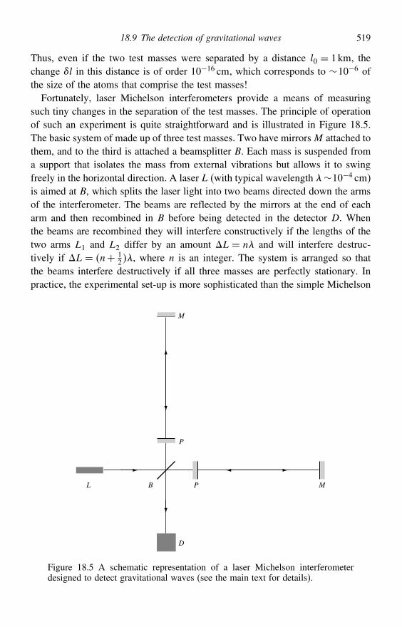
18.9 The detection of gravitational waves 519
Thus, even if the two test masses were separated by a distance l0 = 1km, thechange l in this distance is of order 10−16 cm, which corresponds to ∼10−6 ofthe size of the atoms that comprise the test masses!
Fortunately, laser Michelson interferometers provide a means of measuringsuch tiny changes in the separation of the test masses. The principle of operationof such an experiment is quite straightforward and is illustrated in Figure 18.5.The basic system of made up of three test masses. Two have mirrorsM attached tothem, and to the third is attached a beamsplitter B. Each mass is suspended froma support that isolates the mass from external vibrations but allows it to swingfreely in the horizontal direction. A laser L (with typical wavelength ∼10−4 cm)is aimed at B, which splits the laser light into two beams directed down the armsof the interferometer. The beams are reflected by the mirrors at the end of eacharm and then recombined in B before being detected in the detector D. Whenthe beams are recombined they will interfere constructively if the lengths of thetwo arms L1 and L2 differ by an amount L = n and will interfere destruc-tively if L = n+ 1
2, where n is an integer. The system is arranged so thatthe beams interfere destructively if all three masses are perfectly stationary. Inpractice, the experimental set-up is more sophisticated than the simple Michelson
L
D
B P M
M
P
Figure 18.5 A schematic representation of a laser Michelson interferometerdesigned to detect gravitational waves (see the main text for details).
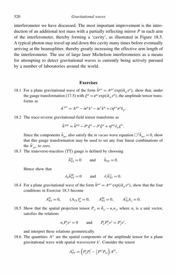
520 Gravitational waves
interferometer we have discussed. The most important improvement is the intro-duction of an additional test mass with a partially reflecting mirror P in each armof the interferometer, thereby forming a ‘cavity’, as illustrated in Figure 18.5.A typical photon may travel up and down this cavity many times before eventuallyarriving at the beamsplitter, thereby greatly increasing the effective arm length ofthe interferometer. The use of large laser Michelson interferometers as a meansfor attempting to detect gravitational waves is currently being actively pursuedby a number of laboratories around the world.
Exercises
18.1 For a plane gravitational wave of the form h = A expikx, show that, under
the gauge transformation (17.5) with = expikx, the amplitude tensor trans-
forms as
A′ = A− ik− ik+ ik
18.2 The trace-reverse gravitational-field tensor transforms as
h′ = h− − +##
Since the components h also satisfy the in vacuo wave equation 2h = 0, showthat this gauge transformation may be used to set any four linear combinations ofthe h′ to zero.
18.3 The transverse-traceless (TT) gauge is defined by choosing
h0iTT = 0 and hTT = 0
Hence show that
0h00TT = 0 and ih
ijTT = 0
18.4 For a plane gravitational wave of the form h =A expikx, show that the four
conditions in Exercise 18.3 become
A0iTT = 0 ATT
= 0 A00
TT = 0 AijTTkj = 0
18.5 Show that the spatial projection tensor Pij ≡ ij −ninj , where ni is a unit vector,satisfies the relations
niPijv
j = 0 and PikP
kj v
j = Pijv
j
and interpret these relations geometrically.18.6 The quantities Aij are the spatial components of the amplitude tensor for a plane
gravitational wave with spatial wavevector ki. Consider the tensor
AijTT =
(PikP
jl − 1
2PijPkl
)Akl
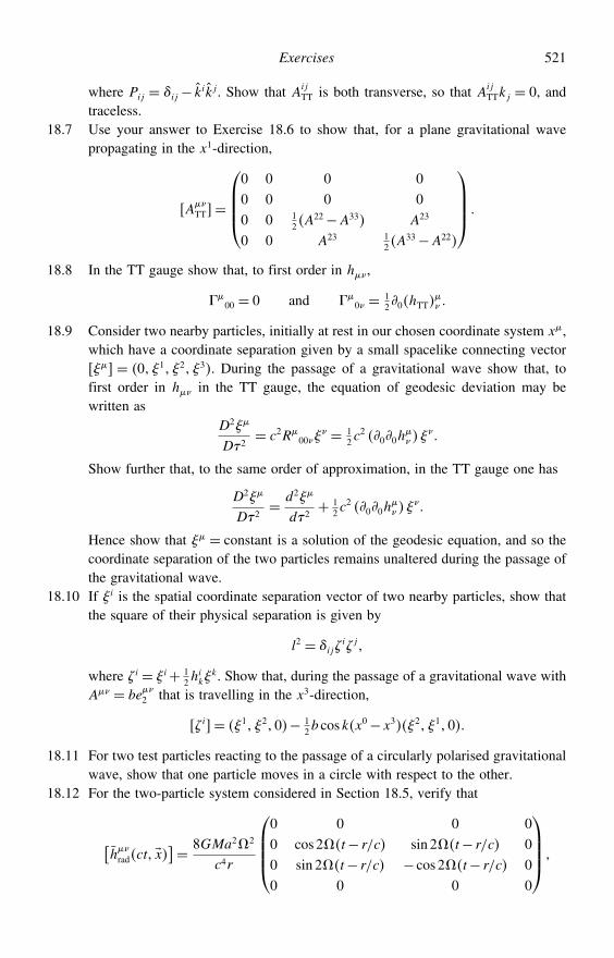
Exercises 521
where Pij = ij − kikj . Show that AijTT is both transverse, so that Aij
TTkj = 0, andtraceless.
18.7 Use your answer to Exercise 18.6 to show that, for a plane gravitational wavepropagating in the x1-direction,
ATT=
⎛⎜⎜⎜⎝0 0 0 0
0 0 0 0
0 0 12 A
22−A33 A23
0 0 A23 12 A
33−A22
⎞⎟⎟⎟⎠
18.8 In the TT gauge show that, to first order in h,
00 = 0 and
0 = 120hTT
18.9 Consider two nearby particles, initially at rest in our chosen coordinate system x,which have a coordinate separation given by a small spacelike connecting vector = 0 1 2 3. During the passage of a gravitational wave show that, tofirst order in h in the TT gauge, the equation of geodesic deviation may bewritten as
D2
D2= c2R
00 = 1
2c2 00h
Show further that, to the same order of approximation, in the TT gauge one has
D2
D2= d2
d2+ 1
2c2 00h
Hence show that = constant is a solution of the geodesic equation, and so thecoordinate separation of the two particles remains unaltered during the passage ofthe gravitational wave.
18.10 If i is the spatial coordinate separation vector of two nearby particles, show thatthe square of their physical separation is given by
l2 = ijij
where i = i+ 12h
ik
k. Show that, during the passage of a gravitational wave withA = be
2 that is travelling in the x3-direction,
i= 1 20− 12b coskx
0−x32 10
18.11 For two test particles reacting to the passage of a circularly polarised gravitationalwave, show that one particle moves in a circle with respect to the other.
18.12 For the two-particle system considered in Section 18.5, verify that
[hradct x
]= 8GMa22
c4r
⎛⎜⎜⎜⎝0 0 0 0
0 cos2t− r/c sin 2t− r/c 0
0 sin 2t− r/c − cos2t− r/c 0
0 0 0 0
⎞⎟⎟⎟⎠
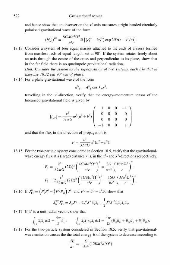
522 Gravitational waves
and hence show that an observer on the x3-axis measures a right-handed circularlypolarised gravitational wave of the form(
hTTrad
) = 8GMa22
c4r [(e1 − ie
2
)exp2it−x3/c
]
18.13 Consider a system of four equal masses attached to the ends of a cross formedfrom massless rods of equal length, set at 90. If the system rotates freely aboutan axis through the centre of the cross and perpendicular to its plane, show thatin the far field there is no quadrupole gravitational radiation.Hint: Consider the system as the superposition of two systems, each like that inExercise 18.12 but 90 out of phase.
18.14 For a plane gravitational wave of the form
hijTT = A
ijTT cos kx
travelling in the x3-direction, verify that the energy–momentum tensor of thelinearised gravitational field is given by
t=c2
32G2a2+b2
⎛⎜⎜⎜⎝1 0 0 −10 0 0 0
0 0 0 0
−1 0 0 1
⎞⎟⎟⎟⎠and that the flux in the direction of propagation is
F = c3
32G2a2+b2
18.15 For the two-particle system considered in Section 18.5, verify that the gravitational-wave energy flux at a (large) distance r is, in the x1- and x3-directions respectively,
F1 =c3
32G22
(4GMa23
c4r
)2
= 2Gc5
(Ma23
r
)2
F3 = 2c3
32G22
(8GMa23
c4r
)2
= 16Gc5
(Ma23
r
)2
18.16 If J ijTT =
(PikP
jl − 1
2PijPkl
)Jkl and Pij = ij− xixj , show that
JTTij J
ijTT = JijJ
ij−2Jji J
ikxj xk+12J ijJklxixj xkxl
18.17 If xi is a unit radial vector, show that∫4xixj d= 4
3ij
∫4xixj xkxl d= 4
15ijkl+ikjl+iljk
18.18 For the two-particle system considered in Section 18.5, verify that gravitational-wave emission causes the the total energy E of the system to decrease according to
dE
dt=− G
5c5128M2a46
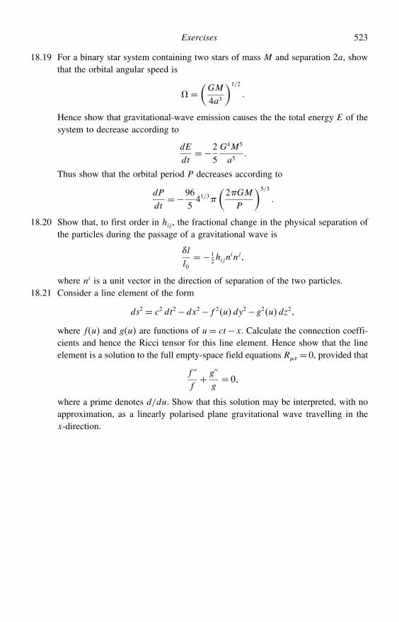
Exercises 523
18.19 For a binary star system containing two stars of mass M and separation 2a, showthat the orbital angular speed is
=(GM
4a3
)1/2
Hence show that gravitational-wave emission causes the the total energy E of thesystem to decrease according to
dE
dt=−2
5G4M5
a5
Thus show that the orbital period P decreases according to
dP
dt=−96
541/3
(2GM
P
)5/3
18.20 Show that, to first order in hij , the fractional change in the physical separation ofthe particles during the passage of a gravitational wave is
l
l0=− 1
2hijninj
where ni is a unit vector in the direction of separation of the two particles.18.21 Consider a line element of the form
ds2 = c2 dt2−dx2−f 2udy2−g2udz2
where fu and gu are functions of u= ct−x. Calculate the connection coeffi-cients and hence the Ricci tensor for this line element. Hence show that the lineelement is a solution to the full empty-space field equations R = 0, provided that
f ′′
f+ g′′
g= 0
where a prime denotes d/du. Show that this solution may be interpreted, with noapproximation, as a linearly polarised plane gravitational wave travelling in thex-direction.
19
A variational approach to general relativity
Most of classical and quantum physics can be expressed in terms of variationalprinciples, and it is often when written in this form that the physical meaningis most clearly understood. Moreover, once a physical theory has been writ-ten as a variational principle it is usually straightforward to identify conservedquantities, or symmetries of the system of interest, that otherwise might havebeen found only with considerable effort. Conversely, by demanding that thevariational principle be invariant under some symmetry, one ensures that theequations of motion derived from it also respect that symmetry. In this finalchapter, we therefore present an introductory account of variational principlesand the Lagrangian formalism. Our ultimate aim will be to derive afresh the fieldequations of general relativity from this new perspective. This will require us toconsider some general aspects of classical field theory in flat and curved space-times. As a result, this chapter lies somewhat outside the mainstream discussionpresented in preceding chapters and may be omitted on a first reading. Never-theless the variational approach that we shall outline is extremely powerful andprovides the basis for most current research into the formulation of classical (andquantum) field theories, including general relativity and other candidate theoriesof gravitation.
19.1 Hamilton’s principle in Newtonian mechanics
To begin, let us remind ourselves of a familiar example of a physical varia-tional principle, namely Hamilton’s principle in Newtonian mechanics. Considera mechanical system whose configuration can be defined uniquely by a numberof generalised coordinates qa, a = 12 n (usually distances and angles),together with time t, and which experiences only forces derivable from a potential.Hamilton’s principle states that in moving from one configuration at time t1 to
524
19.1 Hamilton’s principle in Newtonian mechanics 525
another at time t2 the motion of such a system is such as to make stationary theaction
S =∫ t2
t1
Lqa qa tdt (19.1)
The Lagrangian L is defined, in terms of the kinetic energy T and the potentialenergy V (with respect to some reference situation), by L = T − V . Here V
is a function of the qa (and possibly t) only, but not of the qa. As discussedin Section 3.19, the coordinates define a configuration space with line elementds2 = gab dq
a dqb. For example, the Lagrangian for a particle of mass m can bewritten as
L= T −V = 12mgabq
aqb−V (19.2)
Returning to the general expression (19.1), let us consider an arbitrary variation
qat→ q′at= qat+qat
in the trajectory in configuration space and demand that the corresponding varia-tion S in the action vanishes. Assuming that qat= 0 at the endpoints t1 andt2, we know from our discussion of the calculus of variations in Appendix 3C atthe end of Chapter 3 that the Lagrangian L must satisfy the Euler–Lagrange (EL)equations
L
qa− d
dt
(L
qa
)= 0 a= 12 n
For example, as shown in Section 3.19, the EL equations for the Lagrangian(19.2) are
mqa+ abcq
bqc=−gabbV
which corresponds to Newton’s second law in an arbitrary coordinate system.If the qat are taken to be the Cartesian coordinates xat of the particle, weimmediately recover the more familiar form mxa =−abbV .
Hamilton’s principle is easily extended from the notion of discrete particlesto continuous systems. As an example, let us consider a flexible string stretchedbetween two fixed points at x= 0 and x= l. In this case, we again have one inde-pendent time coordinate t, but now in the context of a continuum in which the qatbecome the continuous variable t x describing the transverse displacementof the string as a function of position and time (see Figure 19.1). Consequently,
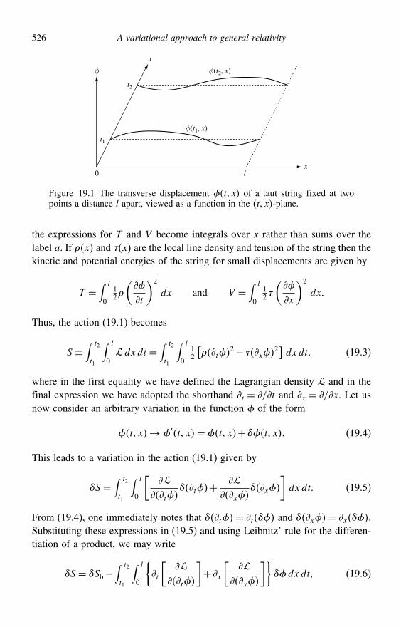
526 A variational approach to general relativity
x
φ
0 l
t1
t2
φ (t2, x)
φ (t1, x)
t
Figure 19.1 The transverse displacement t x of a taut string fixed at twopoints a distance l apart, viewed as a function in the t x-plane.
the expressions for T and V become integrals over x rather than sums over thelabel a. If x and x are the local line density and tension of the string then thekinetic and potential energies of the string for small displacements are given by
T =∫ l
0
12
(
t
)2
dx and V =∫ l
0
12
(
x
)2
dx
Thus, the action (19.1) becomes
S ≡∫ t2
t1
∫ l
0dxdt =
∫ t2
t1
∫ l
0
12
[t
2− x2] dxdt (19.3)
where in the first equality we have defined the Lagrangian density and in thefinal expression we have adopted the shorthand t = /t and x = /x. Let usnow consider an arbitrary variation in the function of the form
t x→ ′t x= t x+t x (19.4)
This leads to a variation in the action (19.1) given by
S =∫ t2
t1
∫ l
0
[
tt+
xx
]dxdt (19.5)
From (19.4), one immediately notes that t= t and x= x.Substituting these expressions in (19.5) and using Leibnitz’ rule for the differen-tiation of a product, we may write
S = Sb−∫ t2
t1
∫ l
0
t
[
t
]+ x
[
x
]dxdt (19.6)
19.2 Classical field theory and the action 527
where the ‘boundary’ (or ‘surface’) term is given by
Sb =∫ t2
t1
∫ l
0
t
[
t
]+ x
[
x
]dxdt
=∫ l
0
[
t
]t=t2t=t1
dx+∫ t2
t1
[
x
]x=lx=0
dt
If we assume that the variation is such that
t1 x= 0= t2 x and t0= 0= t l
then it vanishes on the entire ‘boundary’ of the region of interest in the t x-plane, and we have Sb = 0. Thus, in this case, by demanding that the totalvariation (19.6) in the action vanishes (S = 0) and using the fact that isarbitrary, we obtain
t
[
t
]+ x
[
x
]= tt− xx= 0
where, in the first equality, we have evaluated the derivatives of with respectto t and x using (19.3). If, in addition, and do not depend on x or t then
2
x2= 1
c22
t2
where c2 = /. This is the wave equation for small transverse oscillations of ataut uniform string.
19.2 Classical field theory and the action
In the above discussion, the function t x may be regarded as a ‘field’ definedon a two-dimensional space (or manifold) parameterised by the coordinatesx and t. To extend the idea of a variational principle to a field theory in spacetime,one therefore needs only to replace t x by a (finite) set of fields %ax
defined on a four-dimensional spacetime parameterised in terms of some (ingeneral) arbitrary set of continuous coordinates x. Alternatively, one could evenconsider each member of the (finite) set of generalised coordinates qat in (19.1)as a ‘field’ defined on a one-dimensional manifold parameterised by the continu-ous coordinate t, and simply replace the qat by the set of fields%ax. In eithercase, the index a acts merely as a label for the individual fields in the theory.
This last point is worth clarifying. If, for example, one were considering a fieldtheory containing a set of M scalar fields 12 M then the set of fieldswould be simply !%a"= !12 M". Alternatively, one might be interestedin a field theory containing a vector field (such as electromagnetism). In this
528 A variational approach to general relativity
case, the label a would run over the four components of the vector field in thechosen coordinate system, i.e. we would write !%a" = !A0A1A2A3" = !A"
and so a would then be a spacetime index. Similar considerations apply to thecomponents of tensor fields. Use of the index a may also be trivially extended tolabel the components of two or more vector or tensor fields involved in the theory.Indeed, when considering field theories defined on some arbitrary manifold andin arbitrary coordinates, one must always include the metric tensor componentsin the set of fields. For example, in electromagnetism on an arbitrary manifold,the full set of fields is in fact !%a"= !A g".By analogy with (19.3), the action S for a set of fields defined on some
general four-dimensional spacetime manifold should take the form of an integralof some function , called the Lagrangian density, of the fields %a and theirfirst (and possibly higher) derivatives over some four-dimensional region ofthe spacetime. Thus, we take the action integral to be
S =∫%a %
a %a d4x (19.7)
where d4x denotes the product of coordinate differentials dx0 dx1 dx2 dx3. It isbelieved that physical theories should be generally covariant and so this symmetrymust be reflected in the action S, which therefore has to be a scalar undergeneral coordinate transformations. From the discussion in Section 2.14, we knowthat in any arbitrary coordinate system x the invariant volume element (whichtransforms as a scalar field) is d4V =√−g d4x, where g is the determinant of themetric tensor in that coordinate system (and is negative for the signature of themetric used in this book). It is therefore convenient to write the action (19.7) inthe form
S =∫L√−g d4x
where we have introduced the field Lagrangian L, which is clearly related to theLagrangian density by1
= L√−g (19.8)
For the action S to be a scalar, the quantity L√−g d4x must be a scalar field at
each point in . Since the invariant volume element√−g d4x is already a scalar
field, then so too must be the Lagrangian L. Taking L to be in general a functionof the fields %a and their first (and possibly higher) derivatives, the action for a
1 Although most authors agree that is called the Lagrangian density, it is common in field theory for theterm Lagrangian (and the symbol L) to mean the integral of over some three-dimensional spacelikehypersurface, rather than the relationship given in (19.8). We will adopt the convention (19.8) throughoutthis chapter.
19.3 Euler–Lagrange equations 529
set of classical fields defined on some 4-dimensional spacetime manifold may bewritten as
S =∫L%a %
a %a
√−g d4x
where L is a scalar function of spacetime position. We note finally that theLagrangian density in (19.8) will not transform as a scalar field under coor-dinate transformations; in fact, it is what is known as a scalar density of weightunity, although we need not concern ourselves here with the definition of suchobjects.
19.3 Euler–Lagrange equations
We now derive the form of the field equations for (some subset of) the fields %a
by demanding that the action is stationary, or invariant, under small variations in(the same subset of) the fields of the form
%ax→%′ax=%ax+%ax (19.9)
It is important to note that we are not performing any coordinate transformationhere; we are considering only variations in the functional forms of the fields %a ina fixed coordinate system. For simplicity, we shall perform our derivation of thefield equations under the assumption that the field theory is local, which meansthat second- or higher-order derivatives of the fields do not appear in the action.Thus, we need only consider the consequent variation in the first derivatives ofthe fields, which, from (19.9), is given by
%a→ %
′a = %a+ %
a (19.10)
We also note for later use that, from its definition (19.9), the -operator commuteswith derivatives since
%a= %
′a−%a= %′a− %
a = %a (19.11)
The variations (19.9, 19.10) lead to a variation in the action S→ S+S, with
S =∫d4x =
∫
[
%a%a+
%a%
a
]d4x (19.12)
where, for the time being, it is convenient to work in terms of the Lagrangiandensity defined in (19.8). To derive the field equations, we wish to factor out
530 A variational approach to general relativity
the variation %a in the second term of the integrand. Using (19.11), this secondterm may be written
∫
%a%
ad4x =∫
[
%a%a
]d4x
−∫
[
%a
]%a d4x
where we have integrated by parts (which corresponds simply to rewriting theintegrand using Leibnitz’ theorem for the derivative of a product). The firstintegral on the right-hand side is a total derivative and can therefore be convertedinto an integral over the bounding surface of the region , by straightforwardcalculus. If we restrict the permissible variations %a to those that vanish on theboundary , this integral will also vanish and so (19.12) becomes2
S ≡∫
%a%a d4x =
∫
%a−
[
%a
]%a d4x
where, in the first equality, we define the variational derivative /%a of theLagrangian density with respect to the field %a. If we demand that the action isstationary, so that S = 0, under the arbitrary variations %a we thus require that
%a=
%a−
[
%a
]= 0 (19.13)
These are the Euler–Lagrange (EL) equations, which correspond to the fieldequations of the (local) field theory defined by the action S = ∫d4x. If, inaddition, the Lagrangian density depends on second- or higher-order derivatives ofthe fields then the above derivation is straightforwardly generalised. For example,if second-order derivatives also appear then one obtains
%a=
%a−
[
%a
]+
[
%a
]= 0 (19.14)
provided that the variations %a and their first derivatives vanish on the bound-ary .
2 The restriction that the variation %a vanishes on the boundary is generally allowable, except whendiscussing topological objects in field theory such as instantons, which are beyond the scope of our discussion.
19.4 Alternative form of the Euler–Lagrange equations 531
19.4 Alternative form of the Euler–Lagrange equations
The EL equations in the form (19.13), or generalised to higher-order derivativesof the fields, provide a straightforward means of determing the field equationscorresponding to a given action. In particular, these equations still hold if (someof) the fields %a being varied are the components of the metric tensor g (orfunctions thereof), as will be the case when we derive the Einstein equations fromthe gravitational action in Section 19.8.
Nevertheless, if the fields %a being varied are not functions of the metric tensorcomponents then the presence of the
√−g factor in the Lagrangian density (19.8)makes evaluation of the derivative terms in the EL equations (19.13) unnecessarilycumbersome, although one will nevertheless arrive at the correct field equations.In such cases, however, the Lagrangian L can often be written in terms of thefields %a and their first (and possibly higher-order) covariant derivatives %
a,as opposed to partial derivatives. Indeed, recalling that L should be a scalarfunction of spacetime position, one might expect this to be the case since scalarsare most easily obtained by contracting tensor indices. Let us therefore repeat ourderivation of the form of the EL equations, working instead with an action of theform
S =∫L%a%
a%a g #g
√−g d4x (19.15)
where the fields %a being varied are independent of the metric tensor g butL might still contain g, to raise or lower indices, for example (L might alsocontain the partial derivatives of g; recall that the covariant derivatives of themetric vanish identically).
For simplicity, let us again assume that no second- or higher-order covari-ant derivatives appear in L. The variation (19.9) leads to variations in the firstcovariant derivatives of the fields given by
%a→ %
′a = %a+%
a (19.16)
In a similar way to before, we note that the -operator commutes with covariantderivatives, so that %
a = %a. The variations (19.9–19.16) lead, in
turn, to a variation in the action S→ S+S, with
S=∫L√−g d4x=
∫
[L
%a%a+ L
%a%
a
]√−g d4x (19.17)
where we are now working in terms of the Lagrangian L (as opposed to theLagrangian density ). The partial derivative appearing in the first term ofthe integrand on the right-hand side deserves some comment. In (19.17), we
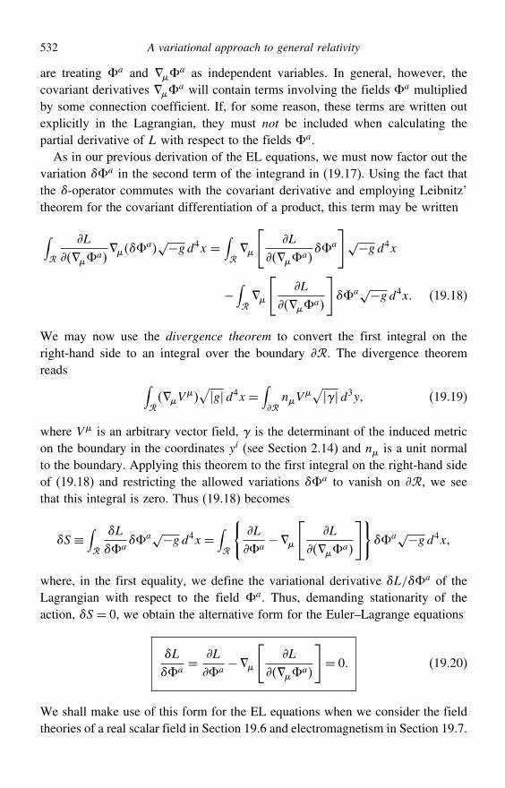
532 A variational approach to general relativity
are treating %a and %a as independent variables. In general, however, the
covariant derivatives %a will contain terms involving the fields %a multiplied
by some connection coefficient. If, for some reason, these terms are written outexplicitly in the Lagrangian, they must not be included when calculating thepartial derivative of L with respect to the fields %a.
As in our previous derivation of the EL equations, we must now factor out thevariation %a in the second term of the integrand in (19.17). Using the fact thatthe -operator commutes with the covariant derivative and employing Leibnitz’theorem for the covariant differentiation of a product, this term may be written
∫
L
%a%
a√−g d4x =
∫
[L
%a%a
]√−g d4x
−∫
[L
%a
]%a√−g d4x (19.18)
We may now use the divergence theorem to convert the first integral on theright-hand side to an integral over the boundary . The divergence theoremreads ∫
V
√gd4x =
∫
nV√d3y (19.19)
where V is an arbitrary vector field, is the determinant of the induced metricon the boundary in the coordinates yi (see Section 2.14) and n is a unit normalto the boundary. Applying this theorem to the first integral on the right-hand sideof (19.18) and restricting the allowed variations %a to vanish on , we seethat this integral is zero. Thus (19.18) becomes
S ≡∫
L
%a%a√−g d4x =
∫
L
%a−
[L
%a
]%a√−g d4x
where, in the first equality, we define the variational derivative L/%a of theLagrangian with respect to the field %a. Thus, demanding stationarity of theaction, S = 0, we obtain the alternative form for the Euler–Lagrange equations
L
%a= L
%a−
[L
%a
]= 0 (19.20)
We shall make use of this form for the EL equations when we consider the fieldtheories of a real scalar field in Section 19.6 and electromagnetism in Section 19.7.
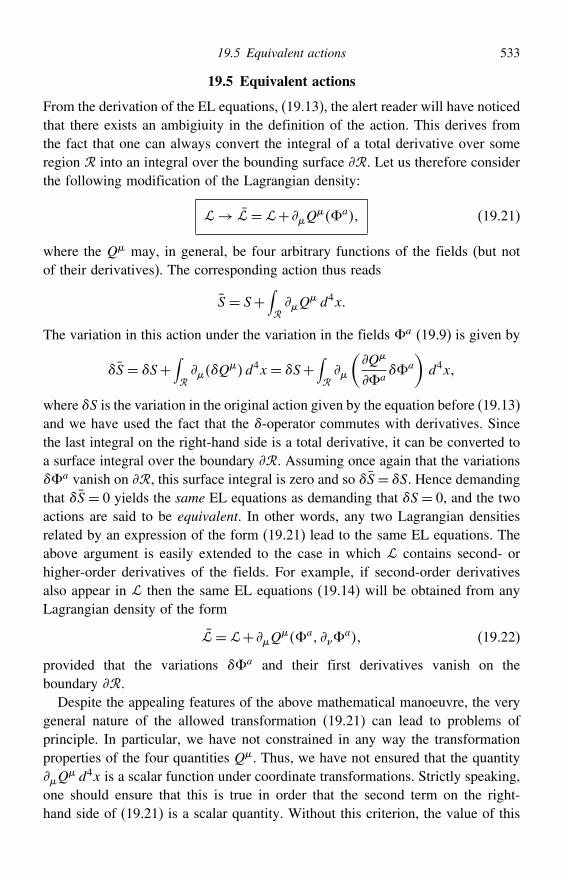
19.5 Equivalent actions 533
19.5 Equivalent actions
From the derivation of the EL equations, (19.13), the alert reader will have noticedthat there exists an ambigiuity in the definition of the action. This derives fromthe fact that one can always convert the integral of a total derivative over someregion into an integral over the bounding surface . Let us therefore considerthe following modification of the Lagrangian density:
→ = + Q%a (19.21)
where the Q may, in general, be four arbitrary functions of the fields (but notof their derivatives). The corresponding action thus reads
S = S+∫Q
d4x
The variation in this action under the variation in the fields %a (19.9) is given by
S = S+∫Q
d4x = S+∫
(Q
%a%a
)d4x
where S is the variation in the original action given by the equation before (19.13)and we have used the fact that the -operator commutes with derivatives. Sincethe last integral on the right-hand side is a total derivative, it can be converted toa surface integral over the boundary . Assuming once again that the variations%a vanish on , this surface integral is zero and so S= S. Hence demandingthat S = 0 yields the same EL equations as demanding that S = 0, and the twoactions are said to be equivalent. In other words, any two Lagrangian densitiesrelated by an expression of the form (19.21) lead to the same EL equations. Theabove argument is easily extended to the case in which contains second- orhigher-order derivatives of the fields. For example, if second-order derivativesalso appear in then the same EL equations (19.14) will be obtained from anyLagrangian density of the form
= + Q%a %
a (19.22)
provided that the variations %a and their first derivatives vanish on theboundary .
Despite the appealing features of the above mathematical manoeuvre, the verygeneral nature of the allowed transformation (19.21) can lead to problems ofprinciple. In particular, we have not constrained in any way the transformationproperties of the four quantities Q. Thus, we have not ensured that the quantityQ
d4x is a scalar function under coordinate transformations. Strictly speaking,one should ensure that this is true in order that the second term on the right-hand side of (19.21) is a scalar quantity. Without this criterion, the value of this
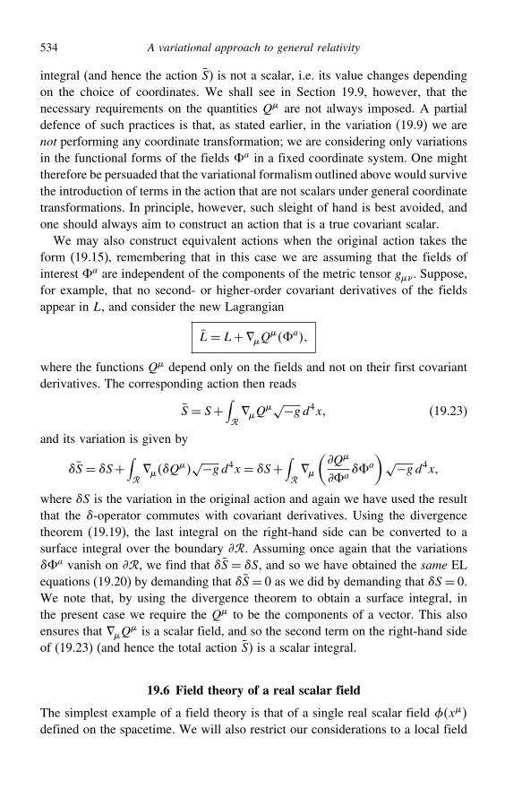
534 A variational approach to general relativity
integral (and hence the action S) is not a scalar, i.e. its value changes dependingon the choice of coordinates. We shall see in Section 19.9, however, that thenecessary requirements on the quantities Q are not always imposed. A partialdefence of such practices is that, as stated earlier, in the variation (19.9) we arenot performing any coordinate transformation; we are considering only variationsin the functional forms of the fields %a in a fixed coordinate system. One mighttherefore be persuaded that the variational formalism outlined above would survivethe introduction of terms in the action that are not scalars under general coordinatetransformations. In principle, however, such sleight of hand is best avoided, andone should always aim to construct an action that is a true covariant scalar.
We may also construct equivalent actions when the original action takes theform (19.15), remembering that in this case we are assuming that the fields ofinterest %a are independent of the components of the metric tensor g. Suppose,for example, that no second- or higher-order covariant derivatives of the fieldsappear in L, and consider the new Lagrangian
L= L+Q%a
where the functions Q depend only on the fields and not on their first covariantderivatives. The corresponding action then reads
S = S+∫Q
√−g d4x (19.23)
and its variation is given by
S = S+∫Q
√−g d4x = S+
∫
(Q
%a%a
)√−g d4x
where S is the variation in the original action and again we have used the resultthat the -operator commutes with covariant derivatives. Using the divergencetheorem (19.19), the last integral on the right-hand side can be converted to asurface integral over the boundary . Assuming once again that the variations%a vanish on , we find that S = S, and so we have obtained the same ELequations (19.20) by demanding that S = 0 as we did by demanding that S = 0.We note that, by using the divergence theorem to obtain a surface integral, inthe present case we require the Q to be the components of a vector. This alsoensures that Q
is a scalar field, and so the second term on the right-hand sideof (19.23) (and hence the total action S) is a scalar integral.
19.6 Field theory of a real scalar field
The simplest example of a field theory is that of a single real scalar field x
defined on the spacetime. We will also restrict our considerations to a local field
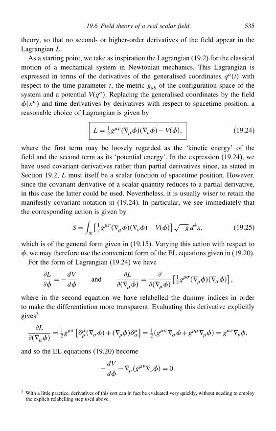
19.6 Field theory of a real scalar field 535
theory, so that no second- or higher-order derivatives of the field appear in theLagrangian L.
As a starting point, we take as inspiration the Lagrangian (19.2) for the classicalmotion of a mechanical system in Newtonian mechanics. This Lagrangian isexpressed in terms of the derivatives of the generalised coordinates qat withrespect to the time parameter t, the metric gab of the configuration space of thesystem and a potential Vqa. Replacing the generalised coordinates by the fieldx and time derivatives by derivatives with respect to spacetime position, areasonable choice of Lagrangian is given by
L= 12g
−V (19.24)
where the first term may be loosely regarded as the ‘kinetic energy’ of thefield and the second term as its ‘potential energy’. In the expression (19.24), wehave used covariant derivatives rather than partial derivatives since, as stated inSection 19.2, L must itself be a scalar function of spacetime position. However,since the covariant derivative of a scalar quantity reduces to a partial derivative,in this case the latter could be used. Nevertheless, it is usually wiser to retain themanifestly covariant notation in (19.24). In particular, we see immediately thatthe corresponding action is given by
S =∫
[ 12g
−V]√−g d4x (19.25)
which is of the general form given in (19.15). Varying this action with respect to, we may therefore use the convenient form of the EL equations given in (19.20).
For the form of Lagrangian (19.24) we have
L
=−dV
dand
L
=
[ 12g
##]
where in the second equation we have relabelled the dummy indices in orderto make the differentiation more transparent. Evaluating this derivative explicitlygives3
L
= 1
2g#[ #+
#
]= 12g
##+g= g
and so the EL equations (19.20) become
−dV
d−g
= 0
3 With a little practice, derivatives of this sort can in fact be evaluated very quickly, without needing to employthe explicit relabelling step used above.
536 A variational approach to general relativity
Remembering that the covariant derivative of the metric tensor is zero, andrearranging, we thus find that the dynamical field equation satisfied by is
2+ dV
d= 0 (19.26)
where 2 ≡ = g is the covariant d’Alembertian operator.A common choice for the potential is V = 1
2m22, where m is a constant
parameter that characterises the dynamics of the scalar field. The field equation(19.26) then becomes
2+m2= 0
which is known as the Klein–Gordon equation. Upon quantisation (which isbeyond the scope of our discussion), this field theory describes collections ofneutral spinless particles of mass m that do not interact with each other exceptthrough their mutual gravitational attraction.
19.7 Electromagnetism from a variational principle
As discussed in Chapter 6, electromagnetism may be described in terms of thevector field A. Thus, using the general description given in Section 19.2, thefields %a a= 1 4 being varied are the components of this vector field andso a is a spacetime index. To describe the dynamics of the electromagnetic fieldin terms of the variational principle, again we begin by constructing a LagrangianL which is a function of A and its first derivatives and which behaves as a scalarfield under general coordinate transformations. We will work from the outsetassuming arbitrary coordinates.
In the case of electromagnetism, however, we saw in Chapter 6 that the theoryalso possesses a gauge invariance. If A describes the electromagnetic field insome physical situation then the same situation is also described by any otherfield of the form
A′ = A+ = A+ (19.27)
where is any scalar field (the last equality holds because the covariant derivativeof the scalar is simply its partial derivative). As discussed earlier, by demandingthat the action be invariant under some symmetry one ensures that the resultingequations of motion also respect that symmetry. We must therefore make surethat the action is invariant under the gauge transformation (19.27). This precludesus from forming scalars depending on AA
, since it is easy to show that this
19.7 Electromagnetism from a variational principle 537
expression is not gauge invariant. Nevertheless, the electromagnetic field-strengthtensor
F = A−A = A− A (19.28)
is easily shown to be gauge invariant; the second equality in (19.28) holds sincea convenient cancellation occurs between the terms containing connection coef-ficients arising from the two covariant derivatives. The most obvious scalar tobe constructed from the field-strength tensor is simply FF
= gg#F#F.Including a factor of−1/40 for later convenience, we shall take the ‘free-field’part of the Lagrangian to be
Lf =−1
40gg#A# −#AA−A
where, again for later convenience, we have written the expression in terms ofcovariant derivatives rather than partial derivatives.
So far we have not taken into account that the source of the electromagneticfield is the 4-current density j of any charged matter present. To describe this,we must include an ‘interaction term’ in the Lagrangian. The most straightforwardscalar we may construct from the electromagnetic field and the current density isjA, and we will take the interaction term to be Li = −jA. Taking the fullLagrangian to be L= Lf +Li, the action reads
S =∫
[− 140
gg#A# −#AA−A− jA
]√−g d4x
(19.29)
As is immediately apparent, however, the interaction term −jA is not auto-matically gauge invariant. Under the gauge transformation (19.27) the correspond-ing term in the action becomes
−∫ jA+ j
√−g d4x =−∫ jA+j
− j
√−g d4x
Using the divergence theorem (19.19), we may write the second term in theintegrand on the right-hand side as a surface integral over the boundary .Taking the source j to vanish on (by, for example, taking the boundary tobe at spatial infinity), the surface integral is zero. Thus, we see that the part ofthe action arising from the interaction term is, in fact, gauge invariant, providedthat the source j satisfies the covariant continuity equation
j = 0
and so the requirement of gauge invariance implies the conservation of charge.
538 A variational approach to general relativity
Thus, under the appropriate conditions, the action (19.29) is invariant underthe gauge transformation (19.27) and, by construction, is a scalar under generalcoordinate transformations. Let us now determine the Euler–Lagrange equationsresulting from varying the fields A in this action (while keeping the sourcej fixed). From (19.29), we see that the action has the general form (19.15).Therefore we may once again use the form of the EL equations given in (19.20),which in this case read
L
A
−
[L
A
]= 0 (19.30)
For the action in (19.29), we have immediately
L
A
=−j =−j (19.31)
but evaluation of the second term on the left-hand side of (19.30) requires morecare. Relabelling dummy indices, and writing A −A = F for conve-nience, we have
L
A=
A
[− 140
gg#F#F
]= − 1
40gg#
[(
# −#
)F+F#
(
−
)]= − 1
40gg−ggF−
140
gg# −gg#F#
= − 140
F−F− 140
F−F=− 10
F
where in the last equality we have used the antisymmetry of the field-strengthtensor (19.28). Combining this result with (19.31), the EL Lagrange equations(19.30) read
F = 0j
which is the same expression as that for the inhomogeneous Maxwell equations inan arbitrary coordinate system, given in Section 7.7. The remaining homogeneousMaxwell equations are in fact automatically satisfied from the definition (19.28)of the field-strength tensor, since
#F+F#+F# = #F+ F#+ F# = 0
Of course, one may object to the fact that we carefully constructed the action(19.29) (by, for example, including specific factors in Lf and Li) in such a way that
19.8 The Einstein–Hilbert action and general relativity in vacuo 539
its variation with respect to A led to the field equations for electromagnetism.Nevertheless, the derivation above illustrates the natural way in which the actionapproach constrains the possible forms for the theory and allows any symmetriesin the theory to be made manifest.
19.8 The Einstein–Hilbert action and general relativity in vacuo
We now use our experience in expressing scalar field theory and electromagnetismas variational principles to construct an action for gravitation from which theEinstein field equations of general relativity can be derived. For the time being,we will restrict our attention to general relativity in vacuo.
To construct an action for general relativity, we must define a Lagrangian L
which is a scalar under general coordinate transformations and which depends onthe components g of the metric tensor (these are now the dynamical fields), andtheir first- and possibly higher-order derivatives. The simplest non-trivial scalarthat can be constructed from the metric and its derivatives is the Ricci scalar R,which depends on g and its first- and second-order derivatives. In fact, R isthe only scalar derivable from the metric tensor that depends on derivatives nohigher than second order. From our knowledge of gravitation as a manifestationof spacetime curvature, we might also expect L to be derived from the curvaturetensor. Thus, in searching for the simplest plausible variational principle forgravitation, one is immediately led to the Einstein–Hilbert action
SEH =∫R√−g d4x (19.32)
Since the corresponding Lagrangian LEH = R now depends on the elementsof the metric tensor, it is more convenient to work in terms of the Lagrangiandensity EH = R
√−g. The resulting EL equations thus take the form (19.13),which in this case reads
g− #
[
#g
]+ #
[
#g
]= 0
Unfortunately, the task of evaluating each term in the above equation involvesa formidable amount of algebra, albeit straightforward. We shall therefore notpursue this approach any further. Instead, we shall derive the corresponding fieldequations by considering directly the variation in the action resulting from avariation in the metric tensor.
Let us therefore consider a variation in the metric tensor given by
g → g+g
540 A variational approach to general relativity
where g and its first derivative vanish on the boundary of the region . Itwill prove useful also to determine the corresponding variation g in the inversemetric components. This is most easily achieved by noting that gg =
and
using the fact that the constant tensor does not change under a variation. Tofirst order in the variation, one may therefore write
gg+gg = 0 (19.33)
Multiplying through by g# , relabelling indices and rearranging, one obtains
g =−gg#g#Writing the Ricci scalar as R= gR, the first-order variation in the Einstein–
Hilbert action (19.32) can be written as
SEH =∫gR
√−g d4x+∫gR
√−g d4x+∫gR
√−gd4x
≡ S1+S2+S3 (19.34)
To derive the field equations, we need to factor out the variation g in thesecond and third integrals. Let us first focus on the second term and write thevariation R in terms of the variation g in the metric tensor. It is in factmore illuminating, and no more work, to determine the variation R#
in thefull curvature tensor, from which the corresponding variation in the Ricci tensorcan be obtained immediately by contraction. The curvature tensor is given by
R# =
#−
#+
#−
#
Let us first consider the variation in the curvature tensor resulting from an arbitraryvariation in the connection coefficients,
# → #
+ #
It is worth noting that the variation # is the difference of two connections
and is therefore a tensor. As is often the case in proving tensor identities, it iseasiest to work in local geodesic coordinates at some arbitrary point P. In such acoordinate system #
P= 0, and so at the point P we have
R# =
( #
)− ( #
)
Moreover, partial derivatives and covariant derivatives coincide at P and so
R# =
( #
)−
( #
) (19.35)
We now see, however, that the quantities on the right-hand side are tensors, andtherefore (19.35) holds not only in geodesic coordinates at P but in any arbitrarycoordinate system. Since the point P was chosen arbitrarily, the result (19.35)
19.8 The Einstein–Hilbert action and general relativity in vacuo 541
thus holds generally and is known as the Palatini equation. The correspondingvariation in the Ricci tensor is obtained by contracting on # and in (19.35)to give
R =
( #
#
)−#
( #
) (19.36)
We may therefore write the second term on the right-hand side of (19.34) as
S2 =∫g
[
( #
#
)−#
( #
)]√−g d4x
=∫
(g #
# −g# #
)√−g d4x
where in the last line we have used the fact that the covariant derivative of themetric vanishes and we have relabelled indices in the second term of the integrand.Using the divergence theorem (19.19), however, we may write S2 as a surfaceintegral over the boundary , which vanishes provided that the variation in theconnection vanishes on the boundary. This means that variations in the metrictensor and in its first derivatives vanish on .
Let us now turn our attention to the third term S3 in (19.34), in which wemust express
√−g in terms of the variation g. Recalling that g = det g,we note that the cofactor of the element g in this determinant is gg. It followsthat
g = ggg =−gggwhere in the second equality we have used the result (19.33). Thus, we have
√−g =− 1
2−g−1/2g =− 12
√−ggg (19.37)
Substituting this expression into the third term S3 in (19.34) and rememberingthat S2 = 0, we finally discover that the variation in the Einstein–Hilbert actionmay be written as
SEH =∫
(R− 1
2gR)g
√−g d4x (19.38)
By demanding that SEH = 0 and using the fact that the variation g is arbitrary,we thus recover Einstein’s field equations in vacuo:
G ≡ R− 12gR= 0 (19.39)
This is an impressive result, since we have obtained the field equations of generalrelativity by varying an action (19.32) to which we were led very naturallyon the grounds of symmetry and simplicity. This illustrates the power of thevariational approach and should be contrasted with the more heuristic approach
542 A variational approach to general relativity
we had to employ in Section 8.4. Moreover, if one were willing to consider morecomplicated actions, the variational formalism suggests how Einstein’s theorymight be modified by adding to the Lagrangian terms proportional to R2R3, etc.The formalism also provides a means for investigating alternative gravitationalLagrangians. For example, the choice L = R#R
# leads to an alternativeself-consistent theory of gravity considered by Eddington.
19.9 An equivalent action for general relativity in vacuo
The Einstein–Hilbert action (19.32) differs from the action (19.25) for scalar fieldtheory and the action (19.29) for electromagnetism in that it depends on second-order derivatives of the dynamical fields. It is therefore of interest to considerwhether the empty-space gravitational field equations can be derived from anaction that depends only on the metric tensor and its first derivatives. As statedin the previous section, however, R is the only scalar derivable from the metrictensor that depends on derivatives no higher than second order, so at first our goalappears unattainable. Nevertheless, as we will show, we may use the notion ofequivalent actions discussed in Section 19.5 to circumvent this difficulty, albeitin a way that results in a new action that is not a scalar under general coordinatetransformations.
The Lagrangian density EH = √−gR in the Einstein–Hilbert action (19.32)may be written as
EH = √−ggR
= √−gg ( ## − #
#+
# #−
##
)= √−gg ( #
# − # #
)− (19.40)
where in the last line we have defined a new Lagrangian density
≡√−g g (
## −
# #
) (19.41)
which clearly depends only on the metric and its first derivatives. (Note that theminus sign in (19.40) is for later convenience.) By relabelling indices and usingLeibnitz’ rule for the differentiation of products, we can write the first term in(19.40) as
√−gg ( ## − #
#
) = √−gg #
# −√−gg# #
−√−gg ## + #
√−gg #
(19.42)
19.10 The Palatini approach for general relativity in vacuo 543
To evaluate the last two terms on the right-hand side, we note that
#√−gg= 1
2−g−1/2g#g+√−g#g (19.43)
Using the result (3.24) derived in Section 3.10, we have #g = 2g # and, since
the covariant derivative of the metric (or its inverse) is zero,
#g = #g
+ #g
+ #g
= 0
Thus, we may write (19.43) as
#√−gg=√−g (
#g−
#g−
#g)
Substituting this result into the last two terms on the right-hand side of (19.42)(contracting on and # for the first of these terms), relabelling indices andsimplifying, one finds that
√−gg ( ## − #
#
)= √−gg #
# −√−gg# #+2
Thus, we finally discover that the Einstein–Hilbert Lagrangian density (19.40)can be written
EH = + √−gg #
# −√−gg# # (19.44)
where is given by (19.41).We see immediately, however, that the second term in (19.44) is a total deriva-
tive, and so EH and are related by an expression of the form (19.22). Thetwo Lagrangian densities are therefore equivalent. As discussed in Section 19.5,variation of the new action
S =∫g
(
## −
# #
)√−g d4x (19.45)
will thus lead to the same field equations as did the Einstein–Hilbert action SEH,provided that the variation in the metric and its first derivative vanish on theboundary . Thus, the variation of (19.45) will again yield Einstein’s fieldequations in vacuo (which may be checked directly), but the action depends onlyon the metric and its first derivatives. There is, however, a price to pay in adoptingthe above result, since the new action S is easily shown not to be a scalar withrespect to general coordinate transformations (see the discussion in Section 19.5).
19.10 The Palatini approach for general relativity in vacuo
A more elegant and illuminating method for obtaining the Einstein field equationsfrom an action depending only on dynamical fields and their first derivatives is
544 A variational approach to general relativity
provided by the Palatini approach, which we now discuss. In this formalism onetreats the metric g and the connection #
as independent fields. In otherwords, one does not assume any explicit relationship between the metric and theconnection.
We begin again with the Einstein–Hilbert Lagrangian density
EH =√−ggR =√−gg(
## − #
#+
# #−
##
)
which we now consider as a function of the metric, the connection and firstderivatives of the connection, i.e. EH = EHg
#
#. Let us first
consider the variation in the action resulting from a variation in the metric alone.This may be written as
SEH =∫√−ggR d
4x
Demanding that SEH = 0 for an arbitrary variation in the metric, we immediatelyfind that
R = 0
which gives the Einstein field equations in vacuo.Let us now consider varying the action with respect to the connection, which
yields
SEH =∫
√−gg R d4x
=∫
√−gg ##−#
#d
4x (19.46)
where in the second line we have used the contracted version (19.36) of thePalatini equation. Using Leibnitz’ theorem for the differentiation of products andrelabelling some dummy indices, we may write (19.46) as
SEH =∫
(g #
# −g# #
)√−g d4x
−∫
[(g
)
− g
]√−g d4x (19.47)
where we note that we have not assumed that the covariant derivative of themetric vanishes, since we have not (yet) specified any relationship between theconnection and the metric. Using the divergence theorem (19.19), we may writethe first integral on the right-hand side of (19.47) as a surface integral over theboundary , which vanishes if we assume that the variation in the connection
19.11 General relativity in the presence of matter 545
vanishes on the boundary. Relabelling some dummy indices in the second integralon the right-hand side of (19.47), we thus find
SEH =∫
(#g
# −g)
√−g d4x (19.48)
Since we are assuming that the manifold is torsionless, the variation in the
connection, although arbitrary, must be symmetric in its lower two indices. As aresult, demanding that SEH = 0 only requires the symmetric part of the term inparentheses in (19.48) to vanish; when contracted with
, the antisymmetricpart will automatically equal zero. Thus, stationarity of the action requires that
12
#g
# + 12
#g
# −g = 0
We thus deduce that #g = 0, which in turn implies that #g = 0. Hence by
demanding stationarity of the Einstein–Hilbert action with respect to variations inthe (symmetric) connection, we have derived that the covariant derivative of themetric must vanish. We may thus write
g = #g#+ #
g#
Cyclically permuting the free indices to obtain similiar expressions for g andg, combining the results and contracting with g# one finds that
= 1
2g#g#+ g# − g
and hence the connection must be the metric connection.
19.11 General relativity in the presence of matter
So far we have confined our attention to deriving the gravitational field equationsin vacuo. We now consider how the full Einstein equations, in the presence ofother (non-gravitational) fields, may be obtained by a variational principle. Inorder to accommodate this generalisation, one simply needs to add an extra termto the action to give
S = 12&
SEH+SM =∫
(12&
EH+M
)d4x (19.49)
where the Einstein–Hilbert action SEH is considered as a function of the metricand of its first- and second-order derivatives (as in Section 19.8). SM is the‘matter’ action for any non-gravitational fields present, and & = 8G/c4. Thefactor 1/2& in (19.49) is chosen for later convenience.
546 A variational approach to general relativity
Let us now consider varying the action with respect to the (inverse) metric, toobtain
12&
EH
g+ M
g= 0
From (19.38), we see that
EH
g=√−gG
where G = R − 12gR is the Einstein tensor. Thus, if we make the bold
assertion that the energy–momentum tensor of the non-gravitational fields (or‘matter’) is given by
T =2√−g
M
g (19.50)
then we recover the full Einstein equations
G =−&T
The definition (19.50) of the ‘matter’ energy–momentum tensor may appear tobe somewhat arbitrary. Nevertheless, as we show in the next section, this tensorhas all the properties required of an energy–momentum tensor.
19.12 The dynamical energy–momentum tensor
The quantities T defined in (19.50) are clearly the components of a tensor, whichis known more properly as the dynamical energy–momentum tensor. From thedefinition we also see immediately that T is a symmetric tensor, as is requiredby the full Einstein equations (19.39). Most importantly, however, we now showthat it obeys the conservation equation T
= 0.From the definition (19.50), the variation in the matter action resulting from a
variation in the metric is given by
SM ≡∫
M
gg d4x = 1
2
∫T g
√−g d4x
= − 12
∫T g
√−g d4x (19.51)
where, in the last equality, we have written SM in terms of the contravariantcomponents T of the energy–momentum tensor for later convenience, using theresult (19.33). Let us now consider making an infinitesimal general coordinatetransformation
x′ = x+x (19.52)
19.12 The dynamical energy–momentum tensor 547
where x is an infinitesimal smooth vector field. Since the action SM is, byconstruction, a covariant scalar, then we must have SM = 0 under the coordinatetransformation. We know, however, that the metric coefficients must transform as
g′x′= x
x′x#
x′g#x =
[−
x] # −
#x g#x (19.53)
= gx−gxx− g#x
#x
(19.54)
to first order in , where we have used the expression (17.3) for the trans-formation matrix corresponding to the infinitesimal coordinate transformation(19.52). We have explicitly included the dependence on x and x′ in (19.54), sinceit is crucial to determining the corresponding variation g. As mentioned inSection 19.3, this variation is only of the functional form of the fields g. Thus,we have
gx≡ g′x−gx =[g′x
′−gx]− [g′x′−g′x
]= [
g′x′−gx
]−#x#g′x
= [g′x
′−gx]−#x#gx
to first order in . Using the expression (19.54) and dropping the explicitdependence on x, we find that
g =−g−g−g =−+
where, in the second equality, we have rewritten the partial derivatives in terms ofcovariant derivatives, cancelled matching terms involving connection coefficientsand used the fact that g = 0.
Substituting this result into (19.51) and remembering that SM = 0 under acoordinate transformation and that T is symmetric, we have
SM =∫T
√−g d4x = 0
Using Leibnitz’ theorem for the covariant differentiation of a product, we write
SM =∫T
√−g d4x−
∫T
√−g d4x = 0 (19.55)
We may use the divergence theorem (19.19) to write the first integral as a surfaceintegral over the boundary in the usual manner. Assuming that the functionsx vanish on the boundary this surface integral vanishes, leaving only thesecond integral in (19.55). Since the x are arbitrary, however, one immediatelyfinds that
T = 0
548 A variational approach to general relativity
and so the covariant divergence of the energy–momentum tensor vanishes, asrequired. Thus, we see that the general covariance of the matter action impliesenergy–momentum conservation in the same way as the gauge invarianceof the action (19.29) for electromagnetism implies charge conservation (seeSection 19.7).
Now that we have shown that the tensor T defined by (19.50) has theappropriate properties of an energy–momentum tensor, we may calculate theexplicit form of this tensor for some specific ‘matter’ actions. Let us begin byconsidering the action (19.25) for a real scalar field . Varying this action nowwith respect to the (inverse) metric, rather than the field , we obtain
S =∫
[ 12g
]√−g
+ [ 12g−V]√−g d4x
=∫
12− 1
2g[ 12g
##−V]
g√−g d4x
where in the last line we have used the expression (19.37) for √−g. Comparing
the above expression with that in (19.51), we immediately see that the energy–momentum tensor for a real scalar field is given by
T = −g
[ 12#
#−V]
which agrees with the expression (16.7) adopted in our discussion of inflation inSection 16.1.
We may also obtain the energy–momentum tensor for the electromagnetic fieldin a similar manner. From (19.29) and (19.28), in the absence of sources we maywrite the action for electromagnetism as
SEM =−1
40
∫gg#F#F
√−g d4x
where F = A− A and so does not depend on the metric. Varying thisaction with respect to the (inverse) metric, we have
SEM = −1
40
∫
[gg#F#F
√−g+F#F#
√−g] d4x
= − 140
∫
(2g#FF# − 1
2gF#F#)g
√−g d4x
where in the second equality we have substituted the expression (19.37) for√−g and relabelled some dummy indices. Comparing the above expression with
Exercises 549
(19.51), we find that the energy–momentum tensor for the electromagnetic fieldis given by
TEM =−−10
(FF
− 14gF#F
#)
which agrees with the expression derived in Exercise 8.3.Finally, we note that in field theory it is common to define also a canonical
energy–momentum tensor, which is based on Noether’s theorem.4 This states thatfor every symmetry of the action there exists a corresponding conserved quantity.In particular, if an action is invariant under a spacetime translation, characterisedby a coordinate transformation of the form x → x+a in which the vectora does not depend on spacetime position, then one can define a tensor S thatobeys S
= 0. It is this tensor that is usually called the canonical energy–momentum tensor. Unfortunately, there are some drawbacks in using it, since itis not necessarily symmetric (although it can be made so) or gauge invariant.
Exercises
19.1 If x and x are the local line density and tension of a string, show that thekinetic and potential energies of the string for small displacements t x are givenby
T =∫ l
0
12
(
t
)2
dx and V =∫ l
0
12
(
x
)2
dx
19.2 In classical field theory, the conjugate field momenta are defined in terms of theLagrangian density by
a ≡
%a
where %a ≡ 0%a and x0 is a timelike coordinate. The Hamiltonian density is then
defined as
≡ a%a−
Use the Euler–Lagrange equations to show that
%a =
a
and a =−
%a
19.3 Consider the quantity
E =∫S d3x
4 See, for example, L. H. Ryder, Quantum Field Theory, Cambridge University Press, 1985.
550 A variational approach to general relativity
where is the Hamiltonian density in Exercise 19.2 and the integral extends oversome spacelike hypersurface S for which x0 = constant. Setting x≡ t xi andusing a dot to denote t, show that
dE
dt=∫S
[
%a%a+
a
a+
i%ai%
a+
t
]d3x
By integrating the third term in the integrand by parts, show that dE/dt = 0provided that does not depend explicitly on t.
19.4 Obtain an expression for the Hamiltonian density for the string in Exercise 19.1.Hence show that the total energy E of the string is given by
E =∫ l
0 dx
and show explicitly that it is a constant of the motion.19.5 A relative tensor of weight w transforms under a coordinate transformation as
′a···b··· = J−w
x′a
xc· · · x
′b
xd c···d···
where J is the Jacobian of the transformation and is given by
J = det[x′a
xb
]
Show that the product of two relative tensors of weights w1 and w2 is a relativetensor of weight w1+w2. Show further that
√−g is a relative scalar of weightw = 1 (called a scalar density).
19.6 For a field theory defined by the action S = ∫d4x show that, if dependson first- and second-order derivatives of the fields, the Euler–Lagrange equationstake the form
%a=
%a−
[
%a
]+
[
%a
]= 0
provided that the variations %a and their first derivatives vanish on the boundary. How do the Euler–Lagrange equations generalise when depends on higher-order derivatives of the fields? What assumptions are required regarding the valueof the variation %a and its derivatives on R?
19.7 Consider a local field theory for which the action has the form
S =∫ %ax %
axd4x
Under an infinitesimal general coordinate transformation x′ = x+ x, thevariation in the action is given by
S =∫′′ %′ax′ %
′ax′d4x′ −∫ %ax %
axd4x
Exercises 551
Adopting the shorthand notation S = ∫′ ′x′d4x′ − ∫xd4x, show that
S =∫ x+x
xd4x =∫!x+ x
x"d4x
where x= ′x′−x and x= ′x−x.19.8 Suppose that the action in Exercise 19.7 is invariant under the given coordinate
transformation, so that S = 0. Since the range of integration can be chosenarbitrarily, show by writing
=
%a%a+
%a%
a
or otherwise, that
%a−
[
%a
]%a+
[
%a%a+
]= 0
Hence show that the invariance of the action under the given coordinate transfor-mation implies that j
= 0, where
j =
%a%a−
[
%a%
a−
]
in which %ax=%′ax′−%ax. This result is known as Noether’s theorem.19.9 Use your answer to Exercise 19.8 to show that invariance of the action under the
infinitesimal translation x′ = x+ implies that S = 0, where
S =
%a%
a−
which is known as the canonical energy–momentum tensor of the fields %a. IsS
necessarily symmetric in and ?19.10 For the field theory considered in Exercise 19.7, use the fact that does not
depend explicitly on the coordinates x to write
=
%a%
a+
%a%
a
By multiplying the Euler–Lagrange equations by %a and summing over a, use
the above result to show directly that S = 0, where S
is the canonicalenergy–momentum tensor given in Exercise 19.9.
19.11 Consider the ‘modified’ energy–momentum tensor
, = S
+ ##
where S is the canonical energy–momentum tensor given in Exercise 19.9 and
# is any tensor that is antisymmetric in # and . Show that ,
= 0 and
that one can always arrange for , to be symmetric in and .
552 A variational approach to general relativity
19.12 Consider a local field theory defined on Minkowski spacetime in an arbitrarycoordinate system x with metric g. The action has the form
S =∫L %ax%
ax gx√−g d4x
where the fields %a are independent of the metric g and L is a scalar undergeneral coordinate transformations. Use the fact that L does not depend explicitlyon x to write
L=L
%a%
a+ L
%a%
a
By multiplying the appropriate form of the Euler–Lagrange equations by %a,
summing over a and noting that covariant derivatives commute in Minkowskispacetime, use the above result to show that S
= 0, where the covariantcanonical energy–momentum tensor S is given by
S = L
%a%a−gL
19.13 Consider the ‘modified’ energy–momentum tensor
, = S
+##
where S is the canonical energy–momentum tensor given in Exercise 19.12 and
# is any tensor that is antisymmetric in # and . Show that, in a flat spacetime,
, = 0 and that one can always arrange for ,
to be symmetric in and .19.14 In a four-dimensional spacetime, use the divergence theorem to show that∫
√−gv d4x =
∫nv
√− d3y
where v is an arbitrary vector field, is the determinant of the induced metricon the boundary in the coordinates yi and n is a unit normal to the boundary.
19.15 Consider complex scalar field = 1+ i2/√2, where ii = 12 are real
scalar fields with potentials of the form V = 12m
22i . Show that the Lagrangian for
may be written as
L= g∗−m∗
where the asterisk denotes the complex conjugate. By varying and ∗ indepen-dently, show that
2+m2= 0 and 2∗ +m2∗ = 0
where 2 ≡ = g is the covariant d’Alembertian operator.19.16 In the theory of electromagnetism in arbitrary coordinates, the field tensor is
defined by F = A−A. Show directly that
F = A− A
Exercises 553
and that
#F+F#+F# = #F+ F#+ F#
Hence show that F automatically satisfies the relation
#F+F#+F# = 0
19.17 If F = A−A, show that
#F+F#+F# = 2R# +R
#+R#A
where R# is the Riemann tensor. Hence use the cyclic identity (??) to show
that the above expression is zero.19.18 An alternative Lagrangian for electromagnetism is given by
L= 140
FF− 1
20
FA−A− jA
where F and A are considered as independent quantities (i.e. no functionalrelationship between them is assumed). By varying the corresponding action withrespect to F and A independently, show that the Euler–Lagrange equationsyield
F = 0j
and F = A−A
19.19 The Lagrangian for a free massive vector field A of mass m is
L=− 14g
g#A# −#AA−A− 12m
2AA
Show that the field equation for A is given by
A−A+m2A = 0
By making use of the fact that covariant derivatives commute in Minkowskispacetime, show that in this case A
= 0 and hence that the field equation canbe written
2A+m2A = 0
where 2 ≡ = g is the covariant d’Alembertian operator. These arecalled the second-order Proca equations.
19.20 An alternative Lagrangian for a free massive vector field A of mass m, is
L= 14FF
− 12F
A−A− 12m
2AA
where F and A are considered as independent quantities. By varying thecorresponding action with respect to F and A independently, show that theEuler–Lagrange equations yield
F+m2A = 0 and F = A−A
which are called the first-order Proca equations.
554 A variational approach to general relativity
19.21 The simplest scalar action for gravity in vacuo that one can construct from themetric tensor alone is
S =∫
√−g d4x
Show that the corresponding field equations are given by√−gg = 0 and clearly
do not constitute a viable theory of gravity.19.22 Under a general infinitesimal coordinate transformation of the form x′ = x+
x, show that
g ≡ g′x−gx=−+
19.23 Consider a general action for gravity in vacuo of the form
S =∫g #g #g d
4x
By considering a general infinitesimal coordinate transformation of the form x′ =x+x, where the x vanish on the boundary , show that the metric andits derivatives must satisfy the differential constraints
(
g
)= 0
where /g is the variational derivative of the Lagrangian density with respectto the metric. Hence show that for the Einstein–Hilbert action these differentialconstraints lead to the contracted Bianchi identities G
= 0.19.24 Show explicitly that the quadratic action
S =∫g
## −
# #√−g d4x
is not a scalar with respect to general coordinate transformations. Show furtherthat varying this action with respect to the metric and its first derivative leads tothe Einstein field equations in vacuo, provided that the variation in the metric andits first derivative vanish on the boundary .
19.25 Obtain an expression for the dynamical energy–momentum tensor of the complexscalar field considered in Exercise 19.15 and that of the massive vector fieldconsidered in Exercise 19.19.
Bibliography
Abramowitz, M. & Stegun, I. A., Handbook of Mathematical Physics, Dover, 1972.Chandrasekhar, S., An Introduction to the Study of Stellar Structure, Dover, 1958.Chandrasekhar, S., The Mathematical Theory of Black Holes, Oxford University Press,
1983.Clarke, C., On the global isometric embedding of pseudo-Riemannian manifolds,
Proceedings of the Royal Society A314, 417–28, 1970.d’Inverno, R., An Introduction to Einstein’s Relativity, Oxford University Press, 1992.
Princeton University Press, 1996.Feynman, R. P., Morinigo, F. B. & Wagner, W. G., Feynman Lectures on Gravitation,
Addison-Wesley, 1995.Foster, J. & Nightingale, J. D., A Short Course in General Relativity, Springer-Verlag,
1995.Islam, J. N., An Introduction to Mathematical Cosmology, Cambridge University Press,
1992.Liddle, A. & Lyth, D., Cosmological Inflation and Large-Scale Structure, Cambridge
University Press, 2000.Misner, C. W., Thorne, K. S. and Wheeler, J. A., Gravitation, Freeman, 1973.Mukhanov, V. F., Feldman, H. A. & Brandenburger, R. H., Theory of cosmological
perturbations, Physics Reports 215, 203–333, 1992.Nash, J., The imbedding problem for Riemannian manifolds, Annals of Mathematics 63,
20–63, 1956.Padmanabhan, T., Structure Formation in the Universe, Cambridge University Press,
1993.Padmanabhan, T., From Gravitons to Gravity: Myths and Reality, abs/grqc/0409089.Peacock, J., Cosmological Physics, Cambridge University Press, 1999.Rindler, W., Relativity: Special, General and Cosmological, Oxford University Press,
2001.Ryder, R. H., Quantum Field Theory, Cambridge University Press, 1985.Schutz, B. F., Geometrical Methods of Mathematical Physics, Cambridge University
Press, 1980.Schutz, B. F., A First Course in General Relativity, Cambridge University Press, 1985.Tanaka, Y. et al., Nature 375, 659, 1995.Wald, R. M., General Relativity, University of Chicago Press, 1984.Weinberg, S., Gravitation and Cosmology, Wiley, 1972.Will, C., Theory and Experiment in Gravitational Physics, Cambridge University Press,
1981.
555
Index
An italic page number indicates that there is a figure related to the topic on this page.
absolute luminosity, 372accelerating observers, 125–8acceleration
and instantaneous rest frames, 126–7in special relativity, 19–20radial, 335three-acceleration, 123uniform, 21universe, 187see also four-acceleration
accretion discsaround compact objects, 240–4, 277radiation efficiency, 215–16, 240, 338
accretion power, of black holes, 216action, 525, 526–7
and classical field theory, 527–9equivalent, 533–4
and general relativity in vacuo, 542–3stationary, 529–30see also Einstein–Hilbert action
advanced time parameter, 255affine connection, 62–4
and metric functions, 65–7definition, 63symmetry, 65transformation properties, 64
affine parameters, 75–6, 117, 120, 221–2, 340geodesics, 76–7
amplitude tensor, 499–500Andromeda galaxy, 355angular diameter distance, 371, 373–4, 411–13angular momentum barrier, 213, 214angular speed
coordinate, 245proper, 245
antiparticles, 275aphelion, 230
Arcminute Cosmology Bolometer Array Receiver(ACBAR), 460
area, manifolds, 38–42atlas, 27
basis tensors, 100basis vectors, 56–9, 69
and coordinate transformations, 60–1Cartesian, 113–14derivatives, 62–4, 84dual, 56–7, 84orthonormal, 59polar coordinates, 83timelike, 152see also coordinate basis vectors
Bianchi identity, 161, 162big-bang origin, 399–400, 404, 409, 419big-bang theory, 394, 398–400big-crunch theory, 395, 398–400binary system, 508–9
compact, 277–9spin-up, 516–17
Birkhoff’s theorem, 202black hole, 240, 270
accretion power, 216angular momenta, 260charged, Reissner–Nordström geometry,
300–2definition, 257detection, 277–9dynamical mass limits, 279existence of, 258, 260formation of and gravitational collapse,
259–64, 277Hawking effect, 274–7in binary systems, 277, 278singularities, 258, 270
556
Page links added automatically. Attention: for a range of pages the link to the upperlimit of the range is incorrect when not all digits of the page number are shown.
Index 557
tidal forces near, 264–5see also Kerr black hole; Schwarzschild black
hole; supermassive black hole; white hole;wormhole
blackbodyenergy spectrum, 276radiation, 388–9temperature, 277
bounce model, 398Boyer–Lindquist coordinates, 318, 319, 320, 322,
344, 347Boyer–Lindquist form, 318Brans–Dicke theory, 191–2, 235, 236Buchdahl’s theorem, 296bug, two-dimensional, confined to two-dimensional
surface, 33–4, 54
calculus of variations, 87–8Cartesian basis vectors, 113–14Cartesian coordinates, 1, 27, 33–5, 320, 346–7, 525
advantages, 128local, 42–4, 46–7, 48, 67–8, 160Lorentz transformation, 112–13Minkowski spacetime, 111–12rotations, 26
Cartesian inertial frames, 47, 112, 122, 141,142, 149
global, 151local, 150–1, 153, 177–8, 179
centre of mass, worldline of, 170centre-of-momentum coordinates, 482, 507centrifugal force, repulsive, 217Cepheid variable, 370Chandrasekhar, Subrahmanyan (1910–95), 259Chandrasekhar limit, 259, 277charge and electromagnetic force, 135–6charge density, 136–7
proper, 508charge density distribution, 508charged particle, equations of motion, 144–5Christoffel symbol, 106
of the first kind, 66of the second kind, 63see also affine connection
circular motion, 209, 335massive particle, 212–13photon, 219–20see also equatorial circular motion
circular orbits, 213, 243–4stable, 214, 215, 243unstable, 214
circularly polarised mode, 507classical field theory, 524
and action, 527–9clocks, ideal, 11cold dark matter (CDM), 387
comoving coordinates, 443, 467nand fundamental observers, 356–9
comoving Hubble distance, 421compact-source approximation, 481–3, 507–8complex functions, analytic continuation, 254components
metric, 83–4mixed, 94, 97tensor, 93–4, 100, 102, 103–4vector field, 73see also contravariant components; covariant
componentsCompton effect, 124Compton scattering, and relativistic collisions,
123–5configuration space, 79, 525congruence of timelike worldlines, 356aconnection coefficients, 85, 202, 244, 317
of general static isotropic metric, 200–1conservation of energy for perfect fluid, 179–81conservation of momentum for perfect fluid,
179–81continuity, equation of, 180contraction, 66
Lorentz, 177tensor, 99–100
contravariant components, 56, 57, 59–60, 68tensors, 93–4, 100
coordinate angular speed, 245acoordinate basis vectors, 57–9, 113–14, 115–16
spacelike, 275timelike, 275
coordinate distance, 371coordinate patches, 27coordinate singularity, 37, 250, 341coordinate transformations, 5, 8
and basis vectors, 60–1infinitesimal general, 468, 469–70manifolds, 28–30tensor, 101–2
coordinates, 26–52arbitrary, 128–31, 142–4, 145, 151, 155–6, 179Boyer–Lindquist, 318, 319, 320, 322, 344, 347characterisation, 248concept of, 27Kruskal, 258, 266–71, 273Minkowski, 297–8momentum, 26non-degenerate, 27Novikov, 254nnull, 248, 258quasi-Minkowski, 467–8, 485spacelike, 248, 249–50, 266, 273tensor, 102–3timelike, 248, 249–50, 256, 258, 266, 273unique values, 27
558 Index
coordinates (cont.)see also Cartesian coordinates; comoving
coordinates; Eddington–Finkelsteincoordinates; inertial coordinates;polar coordinates; Schwarzschildcoordinates
corona, solar, 239cosmic censorship hypothesis, 301, 324cosmic microwave background (CMB)
characterisation, 388–9distribution, 389power spectrum, 459–62
cosmic time, 419cosmological constant, 185–8, 376, 386,
407–8, 432effective, 430size of, 188
cosmological field equations, 386, 392–3, 407,433, 434
derivation, 376–9cosmological fluids
components, 386–9equations of motion, 379–80multiple-component, 381scalar fields as, 431–2
cosmological models, 386–421analytical, 400–8
cosmological parameters, 390–2cosmological principle, 355–6cosmological redshift, 367–8covariant components, 57, 59–60, 81
of tensors, 93–4, 100, 112covariant derivative, 68–70, 85–6
of tensor, 104–7critical density, 392curl, vector field, 71curvature, 33
and geodesic deviation, 165–7and parallel transport, 163–5Gaussian, 161, 171of manifold, 157–8see also spacetime curvature; spatial curvature
curvature density parameter, 391curvature perturbations
and gauge invariance, 446–9evolution, 449–52initial conditions, 452–5normalisation, 452–5power spectrum, 456–7
curvature scalar, see Ricci scalarcurvature spectrum, definition, 456curvature tensor, 75, 158–9, 182, 250, 267
properties, 159–61in Schwarzschild coordinates, 264spherical surfaces, 161, 170
curve in manifold, 27–8
closed timelike, 301, 327non-null, 75–6null, 75–6parametric, 28tangent vector, 55–6
curved spacetime, 181, 244electromagnetism in, 155–6geodesic motion, 188observers in, 152–3tidal forces in, 167–70see also spacetime curvature
cyclic identity, 160cylinder, 34
parallel transport around, 165
d’Alembertian operator, 71, 140, 144, 148,471, 475
covariant, 432, 535dark matter, 387de Sitter model, 398
properties, 407deceleration parameter, 368–71delta function, four-dimensional, 189density parameters, 390–2, 410
curvature, 391evolution, 415–17present-day, 415total, 392
derivativesabsolute, 72of basis vectors, 62–4, 84see also covariant derivative; directional
derivative; intrinsic derivativedevelopment angle, 402differential manifold, 26directional derivative, 56
vectors as, 81–2distance–redshift relation, 411–13divergence, of vector field, 70divergence theorem, 532Doppler effect, 16–18, 240
and relativistic aberration, 120–1formula for, 18
dual basis vectors, 56–7, 84dust, 178, 182
spherically symmetric collapse of, 260–4use of term, 176worldline, 190
eclipseslunar, 235solar, 235
Eddington, Sir Arthur Stanley (1882–1944),235, 542
Eddington–Finkelstein coordinates, 254–9, 303advanced, 258, 261, 262, 270, 303, 346
Index 559
definition, 254–9limitations, 266
and Kerr geometry, 344–6retarded, 270
definition, 257–9limitations, 266
effective potential, 335general relativistic, 214–15Newtonian, 213–14
Einstein, Albert (1879–1955)and cosmological constant, 185–8, 407–8and special relativity, 22–3elevator experiment, 148–50general relativity theory, 150, 233‘On the Electrodynamics of Moving Bodies’
(1905), 22Einstein–Cartan theories, 193Einstein–de-Sitter (EdS) model, 398, 402, 410, 413
radiation-dominated, 420Einstein equations, 176, 181–3
and cosmological term, 185–8and geodesic motion, 188–90exact, 487in empty space, 183, 202limitations, 317non-linearity, 473perturbed, 443–5solving, 196, 198–202, 248, 270
for spherically symmetric geometries, 288–305weak-field limit, 184–5see also gravitational field equations
Einstein–Hilbert actionand general relativity in vacuo, 539–42Lagrangian density, 544stationarity, 545variation, 540
Einstein–Hilbert Lagrangian density, 543, 544Einstein–Maxwell coupled equations, 297–8, 300Einstein–Maxwell formulation of linearised
gravity, 490–2Einstein–Rosen bridge
and wormholes, 271–4structure, 273
Einstein tensor, 162, 183, 442–3, 444, 546linearised, 487
Einstein’s static universe, 407–8electric fields in inertial frames, 141–2electrodynamics, 22, 189–90electromagnetic field, energy–momentum tensor
for, 548–9electromagnetic field equations, 138–9, 176
derivation, 136–7in arbitrary coordinates, 142–4, 155–6simplification, 140–1see also Maxwell’s equations
electromagnetic field tensor, 138, 139, 140, 156
antisymmetric, 136components, 142, 176definition, 136
electromagnetic forces, 148and charge, 135–6
electromagnetic radiation, generation of, 508electromagnetic waves and gravitational waves
compared, 501electromagnetism, 135–46, 508
and Lorentz gauge conditions, 139–41and special relativity, 135consistent theory of, 135from variational principles, 536–9in arbitrary coordinates, 142–4in curved spacetime, 155–6
electron degeneracy pressure, 259elevator experiment, 148–50ellipticity of planetary orbits, 230, 231emitters
four-velocity, 241gravitational redshift, 202–5, 315
empty-space field equations, 288solutions, 198–202, 248
energy, 118–19conservation of, 179–81potential, 535
energy densityof universe, 390, 433of vacuum, 187, 390
energy equation for particle motion, 213–14energy–momentum invariant, 119energy–momentum tensor, 176–8, 182, 188,
192, 484and spacetime curvature, 176canonical, 549dynamical, 546–9for electromagnetic field, 548–9for gravitational field, 486–90, 511–13for matter, 546for multiple-component fluids, 381for perfect fluid, 178–9, 187, 377–9, 432for scalar field, 432, 444–5non-zero, 288, 296–7, 475of vacuum, 187–8symmetry of, 179
epoch, 418, 19inflationary, 433, 437of recombination, 420
equation of continuity, 180equation of state, 292
polytropic, 293equation-of-state parameter, 380equations of motion, 148
and Newtonian gravity, 209Euler’s, 181for charged particles, 144–5
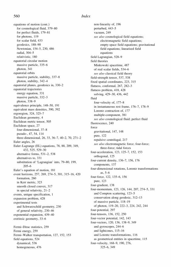
560 Index
equations of motion (cont.)for cosmological fluid, 379–80for perfect fluids, 179–81for photons, 119for scalar field, 433geodesics, 188–90Newtonian, 154–5, 230, 486radial, 304–5relativistic, 180
equatorial circular motionmassive particle, 335–6photon, 341
equatorial orbitsmassive particle, stability, 337–8photon, stability, 342–4
equatorial planes, geodesics in, 330–2equatorial trajectories
energy equation, 331massive particle, 332–3photon, 338–9
equivalence principle, 148–50, 191equivalent mass densities, 390, 392ergoregion, 324, 325–7Euclidean geometry, 4Euclidean metric tensor, 505Euclidean space, 27
four-dimensional, 37–8pseudo-, 47, 54, 114three-dimensional, 26, 33, 36–7, 40–2, 70, 271–2
Euler angles, 26Euler–Lagrange (EL) equations, 78, 88, 209, 349,
432, 525, 529–30alternative forms, 531–2, 538alternatives to, 331substitution of ‘Lagrangian’ into, 79–80, 199,
205–6Euler’s equation of motion, 181event horizons, 257, 269, 274–5, 301, 315–16, 420
formation, 260in Kerr metric, 323smooth closed convex, 317in special relativity, 21–2
events, unique specification, 1expansion problem, 428experimental tests
and Schwarzschild geometry, 230of general relativity, 230–46
exponential expansion, 439–40extrinsic geometry, 33–6
Fermi–Dirac statistics, 259Fermi energy, 259Fermi–Walker transportation, 127, 152, 153field equations, 524
dynamical, 536homogeneous, 476
non-linearity of, 196perturbed, 443–5vacuum, 249see also cosmological field equations;
electromagnetic field equations;empty-space field equations; gravitationalfield equations; linearised fieldequations
field Lagrangian, 528–9field theories
Minkowski spacetime, 487of real scalar fields, 534–6see also classical field theory
field-strength tensor, 537, 538fixed spatial coordinates, 223, 315flatness, conformal, 267, 282–3flatness problem, 418, 428
solving, 429–30, 436, 442fluid
four-velocity of, 177–8in instantaneous rest frame, 176–7, 178–9Lorentz contraction of, 177multiple-component, 381see also cosmological fluid; perfect fluid
fluorescence, 240force
gravitational, 147, 148pure, 122repulsive centrifugal, 217see also electromagnetic force; four-force;
three-force; tidal forcesfour-acceleration, 123, 125–7, 152, 153
orthogonal, 125four-current density, 136–7, 156, 176
components, 137four-dimensional rotations, Lorentz transformations
as, 5–6four-force, 122, 135–6, 156
pure, 123four-gradient, 138four-momentum, 123, 126, 144, 207, 274–5, 331
and Compton scattering, 123–5conservation along geodesic, 312–13of massive particle, 118–19of photon, 119–20, 222–3, 224, 242, 244
four-potential, 297four-tensors, 136, 152, 250four-vector potential, 142, 143four-vectors, 120, 136, 138–9, 349
and gyroscopes, 244–6and lightcones, 115–16and Lorentz transformations, 116as geometrical entities in spacetime, 115
four-velocity, 168–9, 190, 276,325–6, 349
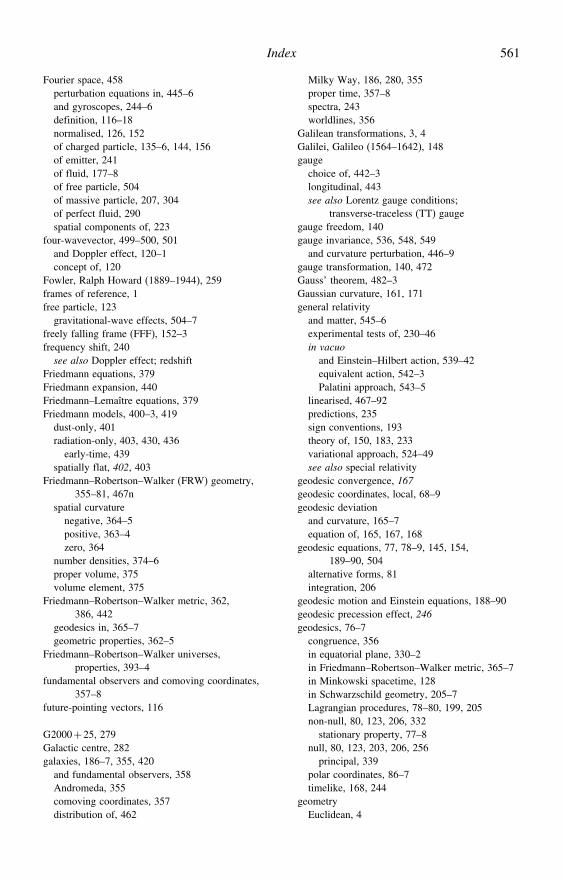
Index 561
Fourier space, 458perturbation equations in, 445–6and gyroscopes, 244–6definition, 116–18normalised, 126, 152of charged particle, 135–6, 144, 156of emitter, 241of fluid, 177–8of free particle, 504of massive particle, 207, 304of perfect fluid, 290spatial components of, 223
four-wavevector, 499–500, 501and Doppler effect, 120–1concept of, 120
Fowler, Ralph Howard (1889–1944), 259frames of reference, 1free particle, 123
gravitational-wave effects, 504–7freely falling frame (FFF), 152–3frequency shift, 240
see also Doppler effect; redshiftFriedmann equations, 379Friedmann expansion, 440Friedmann–Lemaître equations, 379Friedmann models, 400–3, 419
dust-only, 401radiation-only, 403, 430, 436
early-time, 439spatially flat, 402, 403
Friedmann–Robertson–Walker (FRW) geometry,355–81, 467n
spatial curvaturenegative, 364–5positive, 363–4zero, 364
number densities, 374–6proper volume, 375volume element, 375
Friedmann–Robertson–Walker metric, 362,386, 442
geodesics in, 365–7geometric properties, 362–5
Friedmann–Robertson–Walker universes,properties, 393–4
fundamental observers and comoving coordinates,357–8
future-pointing vectors, 116
G2000+25, 279Galactic centre, 282galaxies, 186–7, 355, 420
and fundamental observers, 358Andromeda, 355comoving coordinates, 357distribution of, 462
Milky Way, 186, 280, 355proper time, 357–8spectra, 243worldlines, 356
Galilean transformations, 3, 4Galilei, Galileo (1564–1642), 148gauge
choice of, 442–3longitudinal, 443see also Lorentz gauge conditions;
transverse-traceless (TT) gaugegauge freedom, 140gauge invariance, 536, 548, 549
and curvature perturbation, 446–9gauge transformation, 140, 472Gauss’ theorem, 482–3Gaussian curvature, 161, 171general relativity
and matter, 545–6experimental tests of, 230–46in vacuo
and Einstein–Hilbert action, 539–42equivalent action, 542–3Palatini approach, 543–5
linearised, 467–92predictions, 235sign conventions, 193theory of, 150, 183, 233variational approach, 524–49see also special relativity
geodesic convergence, 167geodesic coordinates, local, 68–9geodesic deviation
and curvature, 165–7equation of, 165, 167, 168
geodesic equations, 77, 78–9, 145, 154,189–90, 504
alternative forms, 81integration, 206
geodesic motion and Einstein equations, 188–90geodesic precession effect, 246geodesics, 76–7
congruence, 356in equatorial plane, 330–2in Friedmann–Robertson–Walker metric, 365–7in Minkowski spacetime, 128in Schwarzschild geometry, 205–7Lagrangian procedures, 78–80, 199, 205non-null, 80, 123, 206, 332
stationary property, 77–8null, 80, 123, 203, 206, 256
principal, 339polar coordinates, 86–7timelike, 168, 244
geometryEuclidean, 4
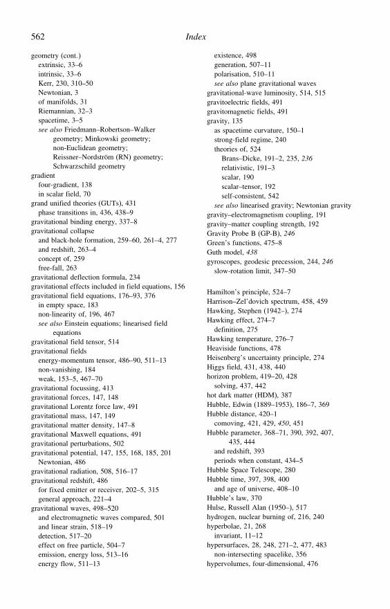
562 Index
geometry (cont.)extrinsic, 33–6intrinsic, 33–6Kerr, 230, 310–50Newtonian, 3of manifolds, 31Riemannian, 32–3spacetime, 3–5see also Friedmann–Robertson–Walker
geometry; Minkowski geometry;non-Euclidean geometry;Reissner–Nordström (RN) geometry;Schwarzschild geometry
gradientfour-gradient, 138in scalar field, 70
grand unified theories (GUTs), 431phase transitions in, 436, 438–9
gravitational binding energy, 337–8gravitational collapse
and black-hole formation, 259–60, 261–4, 277and redshift, 263–4concept of, 259free-fall, 263
gravitational deflection formula, 234gravitational effects included in field equations, 156gravitational field equations, 176–93, 376
in empty space, 183non-linearity of, 196, 467see also Einstein equations; linearised field
equationsgravitational field tensor, 514gravitational fields
energy-momentum tensor, 486–90, 511–13non-vanishing, 184weak, 153–5, 467–70
gravitational focussing, 413gravitational forces, 147, 148gravitational Lorentz force law, 491gravitational mass, 147, 149gravitational matter density, 147–8gravitational Maxwell equations, 491gravitational perturbations, 502gravitational potential, 147, 155, 168, 185, 201
Newtonian, 486gravitational radiation, 508, 516–17gravitational redshift, 486
for fixed emitter or receiver, 202–5, 315general approach, 221–4
gravitational waves, 498–520and electromagnetic waves compared, 501and linear strain, 518–19detection, 517–20effect on free particle, 504–7emission, energy loss, 513–16energy flow, 511–13
existence, 498generation, 507–11polarisation, 510–11see also plane gravitational waves
gravitational-wave luminosity, 514, 515gravitoelectric fields, 491gravitomagnetic fields, 491gravity, 135
as spacetime curvature, 150–1strong-field regime, 240theories of, 524
Brans–Dicke, 191–2, 235, 236relativistic, 191–3scalar, 190scalar–tensor, 192self-consistent, 542
see also linearised gravity; Newtonian gravitygravity–electromagnetism coupling, 191gravity–matter coupling strength, 192Gravity Probe B (GP-B), 246Green’s functions, 475–8Guth model, 438gyroscopes, geodesic precession, 244, 246
slow-rotation limit, 347–50
Hamilton’s principle, 524–7Harrison–Zel’dovich spectrum, 458, 459Hawking, Stephen (1942–), 274Hawking effect, 274–7
definition, 275Hawking temperature, 276–7Heaviside functions, 478Heisenberg’s uncertainty principle, 274Higgs field, 431, 438, 440horizon problem, 419–20, 428
solving, 437, 442hot dark matter (HDM), 387Hubble, Edwin (1889–1953), 186–7, 369Hubble distance, 420–1
comoving, 421, 429, 450, 451Hubble parameter, 368–71, 390, 392, 407,
435, 444and redshift, 393periods when constant, 434–5
Hubble Space Telescope, 280Hubble time, 397, 398, 400
and age of universe, 408–10Hubble’s law, 370Hulse, Russell Alan (1950–), 517hydrogen, nuclear burning of, 216, 240hyperbolae, 21, 268
invariant, 11–12hypersurfaces, 28, 248, 271–2, 477, 483
non-intersecting spacelike, 356hypervolumes, four-dimensional, 476
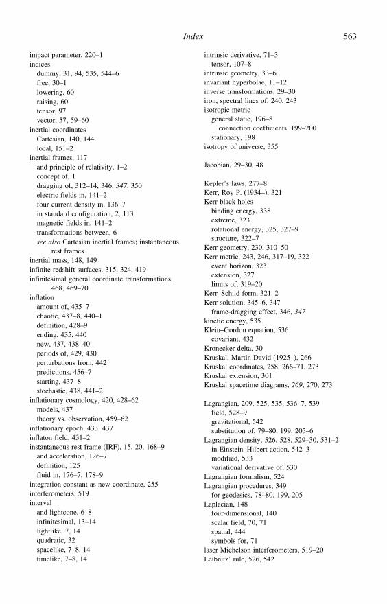
Index 563
impact parameter, 220–1indices
dummy, 31, 94, 535, 544–6free, 30–1lowering, 60raising, 60tensor, 97vector, 57, 59–60
inertial coordinatesCartesian, 140, 144local, 151–2
inertial frames, 117and principle of relativity, 1–2concept of, 1dragging of, 312–14, 346, 347, 350electric fields in, 141–2four-current density in, 136–7in standard configuration, 2, 113magnetic fields in, 141–2transformations between, 6see also Cartesian inertial frames; instantaneous
rest framesinertial mass, 148, 149infinite redshift surfaces, 315, 324, 419infinitesimal general coordinate transformations,
468, 469–70inflation
amount of, 435–7chaotic, 437–8, 440–1definition, 428–9ending, 435, 440new, 437, 438–40periods of, 429, 430perturbations from, 442predictions, 456–7starting, 437–8stochastic, 438, 441–2
inflationary cosmology, 420, 428–62models, 437theory vs. observation, 459–62
inflationary epoch, 433, 437inflaton field, 431–2instantaneous rest frame (IRF), 15, 20, 168–9
and acceleration, 126–7definition, 125fluid in, 176–7, 178–9
integration constant as new coordinate, 255interferometers, 519interval
and lightcone, 6–8infinitesimal, 13–14lightlike, 7, 14quadratic, 32spacelike, 7–8, 14timelike, 7–8, 14
intrinsic derivative, 71–3tensor, 107–8
intrinsic geometry, 33–6invariant hyperbolae, 11–12inverse transformations, 29–30iron, spectral lines of, 240, 243isotropic metric
general static, 196–8connection coefficients, 199–200
stationary, 198isotropy of universe, 355
Jacobian, 29–30, 48
Kepler’s laws, 277–8Kerr, Roy P. (1934–), 321Kerr black holes
binding energy, 338extreme, 323rotational energy, 325, 327–9structure, 322–7
Kerr geometry, 230, 310–50Kerr metric, 243, 246, 317–19, 322
event horizon, 323extension, 327limits of, 319–20
Kerr–Schild form, 321–2Kerr solution, 345–6, 347
frame-dragging effect, 346, 347kinetic energy, 535Klein–Gordon equation, 536
covariant, 432Kronecker delta, 30Kruskal, Martin David (1925–), 266Kruskal coordinates, 258, 266–71, 273Kruskal extension, 301Kruskal spacetime diagrams, 269, 270, 273
Lagrangian, 209, 525, 535, 536–7, 539field, 528–9gravitational, 542substitution of, 79–80, 199, 205–6
Lagrangian density, 526, 528, 529–30, 531–2in Einstein–Hilbert action, 542–3modified, 533variational derivative of, 530
Lagrangian formalism, 524Lagrangian procedures, 349
for geodesics, 78–80, 199, 205Laplacian, 148
four-dimensional, 140scalar field, 70, 71spatial, 444symbols for, 71
laser Michelson interferometers, 519–20Leibnitz’ rule, 526, 542
564 Index
Leibnitz’ theorem, 63, 530, 532, 544, 547Lemaitre models, 393–4
matter-only, 404–6spatially flat, 406–7, 410, 419
properties, 404see also de Sitter model
lengthcoordinate, 39in manifolds, 38–42proper, 10, 39
length contraction, 10–11Lens–Thirring effect, 350Lie derivative, 447nlight, bending of, 233–6, 486, see also speed
of lightlightcones
and four-vectors, 115–16and intervals, 6–8and Schwarzschild solution, 251–2at Schwarzschild radius, 257future-pointing, 477past, 479special-relativistic, 218
line element of Minkowski spacetime, 12–14, seealso Schwarzschild line element
linear strain and gravitational waves, 518–19linear transformations, 2, 46linearised field equations, 467, 470–1,
487, 490–1compact-source approximation, 481–3empty-space, 502far-field solution, 481–3general properties, 473–4general solution, 475–80
multipole expansion for, 480–1in vacuo solution, 474–5static source, 485–6stationary source, 483–5
linearised general relativity, 467–97linearised gravity, 472
Einstein–Maxwell formulation of, 490–2Local Group, 355local theories, 50longitudinal gauge, 443look-back time, 408–10Lorentz contraction of fluid element, 177Lorentz force law, 491
gravitational, 492Lorentz invariant, 137Lorentz symmetry, loss of in general relativity, 487Lorentz transformation matrices, 125Lorentz transformations, 4, 8, 13, 22, 127, 151
and four-vectors, 116and length contraction, 10as four-dimensional rotations, 5–6Cartesian coordinates, 112–13
differentials, 18global, 468, 488homogeneous, 6, 113inertial frames, 313inhomogeneous, 6, 113
Lorentz-boost transformations, 4, 5, 8, 9, 11Lorenz gauge conditions, 501, 510
and electromagnetism, 139–41definition, 140in arbitrary coordinates, 143–4linearised gravity in, 472, 473–4satisfying, 478–9, 498–9, 502, 511–12
luminosityabsolute, 372and gravitational collapse, 263gravitational-wave, 514, 515
luminosity distance, 372–4, 411–12Lynden-Bell, Donald (1935–), 280
Mach’s principle, 149magnetic fields in inertial frames, 141–2magnetohydrodynamic instabilities, 215manifold, 26–52
arbitrary, 528area, 38–42concept of, 26–7coordinate transformations in, 28–30coordinates for, 26curvature of, 157–8differential, 26dimensions, 26flat, 157, 159geometry of, 31length of, 38–42local geometry of, 31one-dimensional, 527pseudo-Euclidean, 111scalar fields, 53Schwarzschild, 272signatures of, 47tangent spaces to, 44–5, 47, 54, 59tensor calculus on, 92–110tensor fields on, 92–3topology, 49–50torsionless, 65, 76two-dimensional, 54–5vector calculus, 53–91vector fields on, 54–5volume, 38–42see also pseudo-Riemannian manifolds;
Riemannian manifolds; submanifoldsMars, Viking lander, 239masers, 281mass function, 278–9massive particle
circular motion, 212–13
Index 565
equatorial, 335–6equatorial trajectories, 332–3four-momentum, 118–19orbits, stability of, 213–17radial motion, 209–11
equatorial initially, 333–5trajectories, 304–5
trajectories, 207–9matter
and general relativity, 545–6baryonic, 387, 391dark, 387energy–momentum tensor, 546non-baryonic, 387
matter-density, 176–7, 387–8, 389, 393gravitational, 147–8
matter-density distribution, quadrupolemoments, 508
matter density perturbationsgrowing mode, 459power spectrum, 458–9
matter power spectrum, 458maximal analytic extension, 301maximally symmetric 3-space, 359–61Maxwell’s equations, 22–3, 139, 141, 176, 189–90,
297–8gravitational, 491homogeneous, 538inhomogeneous, 538predictions, 498see also electromagnetic field equations
MCG-6-30-15, spectra, 243mechanics
Newtonian, 524–7quantum, 259, 274relativistic, 122–3
Mercuryperihelion shift, 233, 235precession, 233retardation, 191
metric components, 83–4metric connection, use of term, 66metric function, 196
and affine connection, 65–7metric tensor, 32, 93, 96, 112Michelson–Morley experiment, 22, 23Milky Way Galaxy, 187, 280–1, 355Minkowski, Hermann (1864–1909), 4Minkowski coordinates, 297–8Minkowski geometry, 5, 26, 317, 319–20
spacetime, 153, 156use of term, 4
Minkowski regions, 269–70Minkowski spacetime, 13, 123, 181, 251, 457, 468
as background, 469, 471, 476n, 484–5, 487, 498coordinate transformations, 5
field theories, 487fixed, 473four-dimensional, 47, 364in arbitrary coordinates, 128–31, 142–4in Cartesian coordinates, 111–12line element, 12–14pseudo-Euclidean, 114, 151symmetries, 486–7tensorial equations, 135weak distortions, 487
Minkowski 2-space, 266–7momentum coordinates, 26Moon, eclipses, 235motion, equations of, see equations of motionM-theory, 271
N Oph 77, 279naked singularities, 301, 324National Aeronautics and Space Administration
(NASA) (US), missions, 246neutrinos, 259, 388neutron, discovery of, 259neutron star, 259–60, 288
gravitational forces, 260in binary system, 277, 278
Newtonian dynamics, 213, 280Newtonian gauge see longitudinal gaugeNewtonian geometry of space and time, 3Newtonian gravity, 147–8, 153, 183, 185, 458
and equations of motion, 208–9and planetary motion, 230and tidal forces, 167–8, 264field equation, 181–2, 186relativistic generalisation, 191
Newtonian limit, 153–5, 180, 182, 185, 393–4, 509and binary systems, 516and static sources, 485–6
Newtonian mechanics, Hamilton’s principle in,524–7
Newtonian potential, 443Newtonian theory, 147, 154–5, 180, 181, 183, 230
and special relativity compared, 2of stellar structure, 288
Newton’s laws of motion, 1NGC 4258, 281Nobel Prize, 517Noether’s theorem, 549non-Euclidean geometry, 4
examples, 36–8non-Euclidean space
infinite, 42three-dimensional, 38, 41–2
non-inertial frames, 129normalised scale parameter, 389Novikov coordinates, 254nnull curve, 75–6
566 Index
null-cone, 116number densities
in Friedmann–Robertson–Walker geometry,374–6
proper, 375–6
observersaccelerating, 125–8in curved spacetime, 152–3fundamental, 356–7
Oppenheimer–Volkoff equation, 293, 294Oppenheimer–Volkoff limit, 260orbit
Newtonian, 208non-circular, 216–17, 230of massive particle, 212–17shape of, 208spiral, 215, 217see also circular orbits; equatorial orbits; photon
orbits; planetary orbitsorthogonal connecting vectors, 170orthogonal coordinates, 39orthonormal basis vectors, 59
Palatini approach for general relativity in vacuo,543–5
Palatini equation, 541, 544parallel transport, 222
and curvature, 163–5and gyroscopes, 244of tensor, 108of vector, 73–5on spherical surface, 165path dependence, 74–5
particlecharged, 144–5four-momentum, 312–13infalling, 210–11, 219, 252–9non-interacting, 176tunnelling, 275see also free particle; massive particle
particle–antiparticle pairs, 274particle horizon, 418–20particle worldlines, 14–16, 116–17, 154, 156
radial, in Schwarzschild coordinates, 252–4past-pointing vectors, 116Pauli exclusion principle, 259Penrose, Sir Roger (1931–), 260, 301,
324, 325Penrose process, 327–9, 344perfect fluid, 289, 386–9
and weak-field limit, 184–5conservation of energy–momentum, 179–81definition, 178–9energy–momentum tensors, 178–9, 187,
376–9, 432
equations of motion, 180–1four-velocity, 290
perihelion, 230shift, 233, 235, 486
perturbation equations, in Fourier space, 445–6perturbations
from inflation, 442gravitational, 502Newtonian potential, 443scalar-field, evolution, 442–6see also curvature perturbations; matter density
perturbationsphase transitions, 430–1photon, 388
circular motion, 219equatorial, 341
equation of motion, 119four-momentum, 119–20, 222, 223, 241, 243four-wavevector, 120–1radial motion, 218–19, 302–4radially outgoing, 257–8redshift, 204–5, 240, 243, 408trajectories, 217, 233–4
equatorial, 338–9photon orbits
circular, 233energy equation, 219–20, 236–7equatorial, stability of, 342–4general, 220stability of, 220–1
photon path deflection, 237–9photon propagation, 342–3, 344photon worldlines, 14, 218, 242, 256
radial, in Schwarzschild coordinates, 251–2Planck era, 430–1, 436Planck scales, 270–1plane gravitational waves
and polarisation states, 498–500effects on free particles, 504–7propagation, 505
planetary motion and Newtonian gravity, 231planetary orbits
ellipticity, 230, 231precession, 230–3
Poincaré transformations, 6, 7, 113Poisson’s equation, 147, 183, 185, 458polar coordinates
cylindrical, 272in a plane, 82–7
polarisation states and plane gravitational waves,498–500
polarisation tensors, linear, 500, 511polytropic index, 293position coordinates, 26potential energy, 535potential functions, 443
Index 567
power spectrumcosmic microwave background, 459–62curvature perturbations, 456–7definition, 456matter density perturbations, 458–9scale invariant, 456
precessiongeodesic, 244–6gyroscopes, 244–6
slow-rotation limit, 347–50planetary orbits, 230–3
primordial spectral index, 457–2, 458principal photon geodesics, equatorial, 339–41principle of relativity and inertial frames, 1–2principal stresses, 170projectiles and elevator experiment, 148–9proper angular speed, 245proper charge density, 508proper density, 509proper distance, 371proper length, 10, 39proper mass density, 508proper motion of stars, 280–1proper number densities, 375–6proper time, 14–16, 204, 206–7, 219, 252–3
finite, 211, 254infinite, 211, 254
proper volume, 10protons, 259
Schwarzschild radius, 249pseudo-Euclidean geometry, see Minkowski
geometrypseudo-Euclidean manifolds, four-dimensional, 111pseudo-Euclidean space, 47, 54, 114pseudo-Riemannian manifold, 39, 45–7, 53, 54,
59, 157curved spacetime, 150–1local Cartesian coordinates, 46–7, 67–8non-null curve, 75null curve, 75use of term, 32vectors, 62, 74
pseudotensors, use of term, 468PSR B1913+16 (binary pulsar), 517–18pulsars, binary, 516–17pulsation, radial, 202
quadratic intervals, 32quadrupole formula, 483, 507–8quadrupole-moment tensor, 483, 508, 509–10,
514, 516reduced, 514, 516
quadrupole moments, transverse-traceless, 514–15quantum chromodynamics and inflation, 431quantum gravity, theory, 188quantum mechanics and white dwarfs, 259, 274
quark–hadron phase transition, 431quasars
discovery, 279–80radio-wave deflection measurements, 236
quasi-Minkowski coordinates, 467–8, 485quasi-stellar objects (QSOs), 279nquotient theorem, 103–4
radar echoes, 236–9radial coordinates, 209radial distance, 209radial motion
equatorial initially, massive particle, 333–5massive particle, 209–11photon, 218–19
radiation density, 388–9, 393radiation efficiency in accretion discs, 215–16,
240, 338radio quasars, 235radio sources, 235rapidities, addition of, 19rapidity parameter, 5, 18receiver and emitter fixed, gravitational redshift,
202–5, 315recombination, 420red giants, 288redshift, 187, 191, 395, 411
and gravitational collapse, 262–3and Hubble parameter, 393cosmological, 355–6infinite, 315, 324, 419photon, 204–5, 240, 242, 408quasar, 279–80see also gravitational redshift
reheating, 451use of term, 435
Reissner–Nordström (RN) black hole, extreme, 301Reissner–Nordström geometry
charged black hole, 300–2radial massive particle trajectories, 304–5radial photon trajectories, 302–4spacetime diagram, 303
relative three-vector, 117relativistic aberration
and Doppler effect, 120–1formula, 121
relativistic collisions and Compton scattering,123–5
relativistic gravitational equationsstatic spherically symmetric charged body, 288,
296–300stellar interior, 288–92stellar structure, 292–4
relativistic mechanics, 122–3relativistic theories of gravity, 191–3r-equation replacement, 206, 217
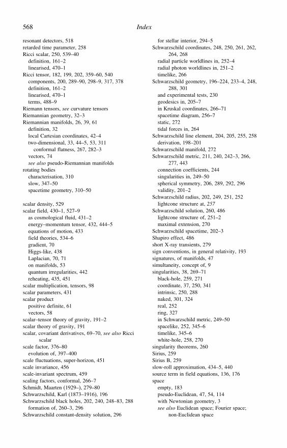
568 Index
resonant detectors, 518retarded time parameter, 258Ricci scalar, 250, 539–40
definition, 161–2linearised, 470–1
Ricci tensor, 182, 199, 202, 359–60, 540components, 200, 289–90, 298–9, 317, 378definition, 161–2linearised, 470–1terms, 488–9
Riemann tensors, see curvature tensorsRiemannian geometry, 32–3Riemannian manifolds, 26, 39, 61
definition, 32local Cartesian coordinates, 42–4two-dimensional, 33, 44–5, 53, 311
conformal flatness, 267, 282–3vectors, 74see also pseudo-Riemannian manifolds
rotating bodiescharacterisation, 310slow, 347–50spacetime geometry, 310–50
scalar density, 529scalar field, 430–1, 527–9
as cosmological fluid, 431–2energy–momentum tensor, 432, 444–5equations of motion, 433field theories, 534–6gradient, 70Higgs-like, 438Laplacian, 70, 71on manifolds, 53quantum irregularities, 442reheating, 435, 451
scalar multiplication, tensors, 98scalar parameters, 431scalar product
positive definite, 61vectors, 58
scalar–tensor theory of gravity, 191–2scalar theory of gravity, 191scalar, covariant derivatives, 69–70, see also Ricci
scalarscale factor, 376–80
evolution of, 397–400scale fluctuations, super-horizon, 451scale invariance, 456scale-invariant spectrum, 459scaling factors, conformal, 266–7Schmidt, Maarten (1929–), 279–80Schwarzschild, Karl (1873–1916), 196Schwarzschild black holes, 202, 240, 248–83, 288
formation of, 260–3, 296Schwarzschild constant-density solution, 296
for stellar interior, 294–5Schwarzschild coordinates, 248, 250, 261, 262,
264, 268radial particle worldlines in, 252–4radial photon worldlines in, 251–2timelike, 266
Schwarzschild geometry, 196–224, 233–4, 248,288, 301
and experimental tests, 230geodesics in, 205–7in Kruskal coordinates, 266–71spacetime diagram, 256–7static, 272tidal forces in, 264
Schwarzschild line element, 204, 205, 255, 258derivation, 198–201
Schwarzschild manifold, 272Schwarzschild metric, 211, 240, 242–3, 266,
277, 443connection coefficients, 244singularities in, 249–50spherical symmetry, 206, 289, 292, 296validity, 201–2
Schwarzschild radius, 202, 249, 251, 252lightcone structure at, 257
Schwarzschild solution, 260, 486lightcone structure of, 251–2maximal extension, 270
Schwarzschild spacetime, 202–3Shapiro effect, 486short X-ray transients, 279sign conventions, in general relativity, 193signatures, of manifolds, 47simultaneity, concept of, 9singularities, 38, 269–71
black-hole, 259, 271coordinate, 37, 250, 341intrinsic, 250, 288naked, 301, 324real, 252ring, 327in Schwarzschild metric, 249–50spacelike, 252, 345–6timelike, 345–6white-hole, 258, 270
singularity theorems, 260Sirius, 259Sirius B, 259slow-roll approximation, 434–5, 440source term in field equations, 136, 176space
empty, 183pseudo-Euclidean, 47, 54, 114with Newtonian geometry, 3see also Euclidean space; Fourier space;
non-Euclidean space
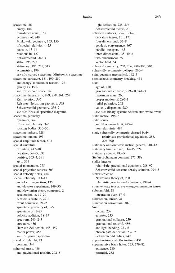
Index 569
spacetime, 26empty, 184four-dimensional, 158geometry of, 240Minkowski geometry, 153, 156of special relativity, 1–25paths in, 13–14rotations in, 127Schwarzschild, 202–3static, 196, 273stationary, 196, 275, 315symmetries, 196see also curved spacetime; Minkowski spacetime
spacetime curvature, 181, 190, 250and energy–momentum tensors, 176gravity as, 150–1see also curved spacetime
spacetime diagrams, 7, 8–9, 258, 261, 267Kerr solution, 346Reissner–Nordström geometry, 303Schwarzschild geometry, 256–7see also Kruskal spacetime diagrams
spacetime geometrydynamics, 376of special relativity, 3–5rotating bodies, 310–50
spacetime indices, 528spacetime torsion, 193spatial amplitude tensor, 503spatial curvature
evolution, 417–18negative, 364–5, 391positive, 363–4, 391zero, 364
spatial momentum, 275spatial projection tensors, 503spatial velocity fields, 484special relativity, 111–13
and electromagnetism, 135and elevator experiment, 149–50and Newtonian theory compared, 2acceleration in, 19–20Einstein’s route to, 22–3event horizon in, 21–2spacetime geometry of, 3–5spacetime of, 1–25velocity addition, 18–19spectrum, 240, 243curvature, 456Harrison-Zel’dovich, 458, 459matter power, 458see also power spectrum
speed of light, 14, 23constant, 3–4
spherical mass, 486and gravitational redshift, 202–5
light deflection, 235, 236Schwarzschild metric, 201
spherical surfaces, 36–7, 171–2curvature tensor, 161, 171four-dimensional, 37–8geodesic convergence, 167parallel transport, 165three-dimensional, 35, 40–2two-dimensional, 35vector field, 54
spherical symmetry, 202, 206, 288–305, 310spherically symmetric collapse, 260–4spin, quantum mechanical, 192–3spontaneous symmetry breaking, 431stars
age of, 410gravitational collapse, 259–60, 261–3maximum mass, 260proper motion of, 280–1radial pulsation, 202velocity dispersion, 280see also binary system; neutron star; white dwarf
static metric, 196–7static source
and Newtonian limit, 485–6non-relativistic, 484
static spherically symmetric charged body,relativistic gravitational equations, 288,296–300
stationary axisymmetric metric, general, 310–12stationary limit surface, 314–15, 324stationary source, 483–5Stefan–Boltzmann constant, 277, 388stellar interior
relativistic gravitational equations, 288–92Schwarzschild constant-density solution, 294–5
stellar structureNewtonian theory of, 288relativistic gravitational equations, 292–4
stress–energy tensor, see energy–momentum tensorsubmanifold, 28
integration over, 47–9subtraction, tensor, 98summation convention, 30–1Sun
corona, 239eclipses, 235gravitational collapse, 259gravitational redshift, 486and light bending, 233–6photon path deflection, 237–9Schwarzschild radius, 249
super-horizon scale fluctuations, 451supermassive black holes, 265, 279–82
existence, 280potential, 282
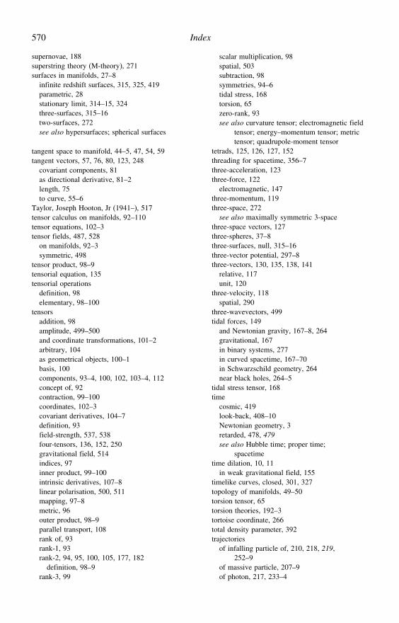
570 Index
supernovae, 188superstring theory (M-theory), 271surfaces in manifolds, 27–8
infinite redshift surfaces, 315, 325, 419parametric, 28stationary limit, 314–15, 324three-surfaces, 315–16two-surfaces, 272see also hypersurfaces; spherical surfaces
tangent space to manifold, 44–5, 47, 54, 59tangent vectors, 57, 76, 80, 123, 248
covariant components, 81as directional derivative, 81–2length, 75to curve, 55–6
Taylor, Joseph Hooton, Jr (1941–), 517tensor calculus on manifolds, 92–110tensor equations, 102–3tensor fields, 487, 528
on manifolds, 92–3symmetric, 498
tensor product, 98–9tensorial equation, 135tensorial operations
definition, 98elementary, 98–100
tensorsaddition, 98amplitude, 499–500and coordinate transformations, 101–2arbitrary, 104as geometrical objects, 100–1basis, 100components, 93–4, 100, 102, 103–4, 112concept of, 92contraction, 99–100coordinates, 102–3covariant derivatives, 104–7definition, 93field-strength, 537, 538four-tensors, 136, 152, 250gravitational field, 514indices, 97inner product, 99–100intrinsic derivatives, 107–8linear polarisation, 500, 511mapping, 97–8metric, 96outer product, 98–9parallel transport, 108rank of, 93rank-1, 93rank-2, 94, 95, 100, 105, 177, 182
definition, 98–9rank-3, 99
scalar multiplication, 98spatial, 503subtraction, 98symmetries, 94–6tidal stress, 168torsion, 65zero-rank, 93see also curvature tensor; electromagnetic field
tensor; energy–momentum tensor; metrictensor; quadrupole-moment tensor
tetrads, 125, 126, 127, 152threading for spacetime, 356–7three-acceleration, 123three-force, 122
electromagnetic, 147three-momentum, 119three-space, 272
see also maximally symmetric 3-spacethree-space vectors, 127three-spheres, 37–8three-surfaces, null, 315–16three-vector potential, 297–8three-vectors, 130, 135, 138, 141
relative, 117unit, 120
three-velocity, 118spatial, 290
three-wavevectors, 499tidal forces, 149
and Newtonian gravity, 167–8, 264gravitational, 167in binary systems, 277in curved spacetime, 167–70in Schwarzschild geometry, 264near black holes, 264–5
tidal stress tensor, 168time
cosmic, 419look-back, 408–10Newtonian geometry, 3retarded, 478, 479see also Hubble time; proper time;
spacetimetime dilation, 10, 11
in weak gravitational field, 155timelike curves, closed, 301, 327topology of manifolds, 49–50torsion tensor, 65torsion theories, 192–3tortoise coordinate, 266total density parameter, 392trajectories
of infalling particle of, 210, 218, 219,252–9
of massive particle, 207–9of photon, 217, 233–4
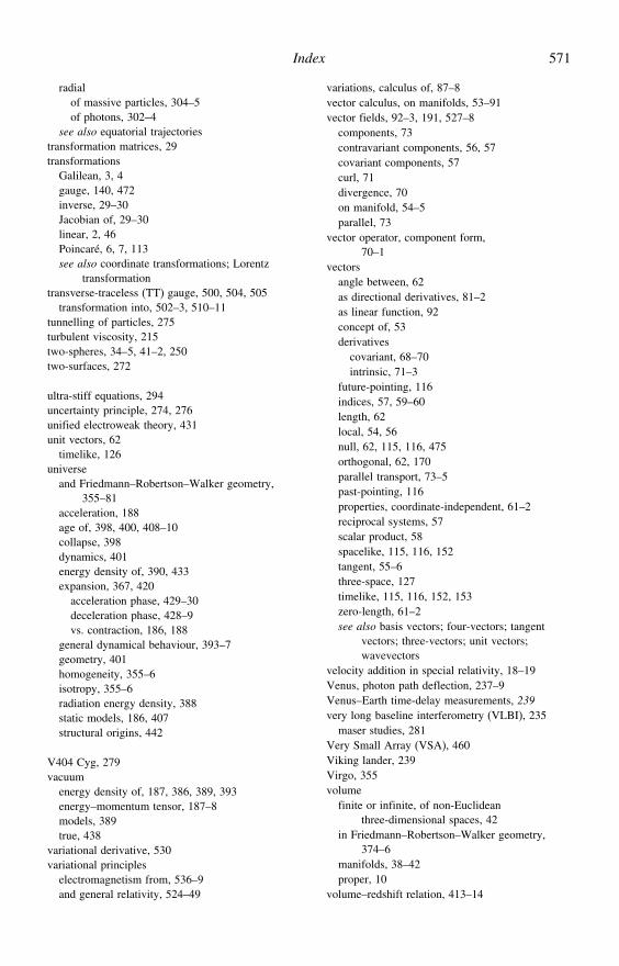
Index 571
radialof massive particles, 304–5of photons, 302–4
see also equatorial trajectoriestransformation matrices, 29transformations
Galilean, 3, 4gauge, 140, 472inverse, 29–30Jacobian of, 29–30linear, 2, 46Poincaré, 6, 7, 113see also coordinate transformations; Lorentz
transformationtransverse-traceless (TT) gauge, 500, 504, 505
transformation into, 502–3, 510–11tunnelling of particles, 275turbulent viscosity, 215two-spheres, 34–5, 41–2, 250two-surfaces, 272
ultra-stiff equations, 294uncertainty principle, 274, 276unified electroweak theory, 431unit vectors, 62
timelike, 126universe
and Friedmann–Robertson–Walker geometry,355–81
acceleration, 188age of, 398, 400, 408–10collapse, 398dynamics, 401energy density of, 390, 433expansion, 367, 420
acceleration phase, 429–30deceleration phase, 428–9vs. contraction, 186, 188
general dynamical behaviour, 393–7geometry, 401homogeneity, 355–6isotropy, 355–6radiation energy density, 388static models, 186, 407structural origins, 442
V404 Cyg, 279vacuum
energy density of, 187, 386, 389, 393energy–momentum tensor, 187–8models, 389true, 438
variational derivative, 530variational principles
electromagnetism from, 536–9and general relativity, 524–49
variations, calculus of, 87–8vector calculus, on manifolds, 53–91vector fields, 92–3, 191, 527–8
components, 73contravariant components, 56, 57covariant components, 57curl, 71divergence, 70on manifold, 54–5parallel, 73
vector operator, component form,70–1
vectorsangle between, 62as directional derivatives, 81–2as linear function, 92concept of, 53derivatives
covariant, 68–70intrinsic, 71–3
future-pointing, 116indices, 57, 59–60length, 62local, 54, 56null, 62, 115, 116, 475orthogonal, 62, 170parallel transport, 73–5past-pointing, 116properties, coordinate-independent, 61–2reciprocal systems, 57scalar product, 58spacelike, 115, 116, 152tangent, 55–6three-space, 127timelike, 115, 116, 152, 153zero-length, 61–2see also basis vectors; four-vectors; tangent
vectors; three-vectors; unit vectors;wavevectors
velocity addition in special relativity, 18–19Venus, photon path deflection, 237–9Venus–Earth time-delay measurements, 239very long baseline interferometry (VLBI), 235
maser studies, 281Very Small Array (VSA), 460Viking lander, 239Virgo, 355volume
finite or infinite, of non-Euclideanthree-dimensional spaces, 42
in Friedmann–Robertson–Walker geometry,374–6
manifolds, 38–42proper, 10
volume–redshift relation, 413–14
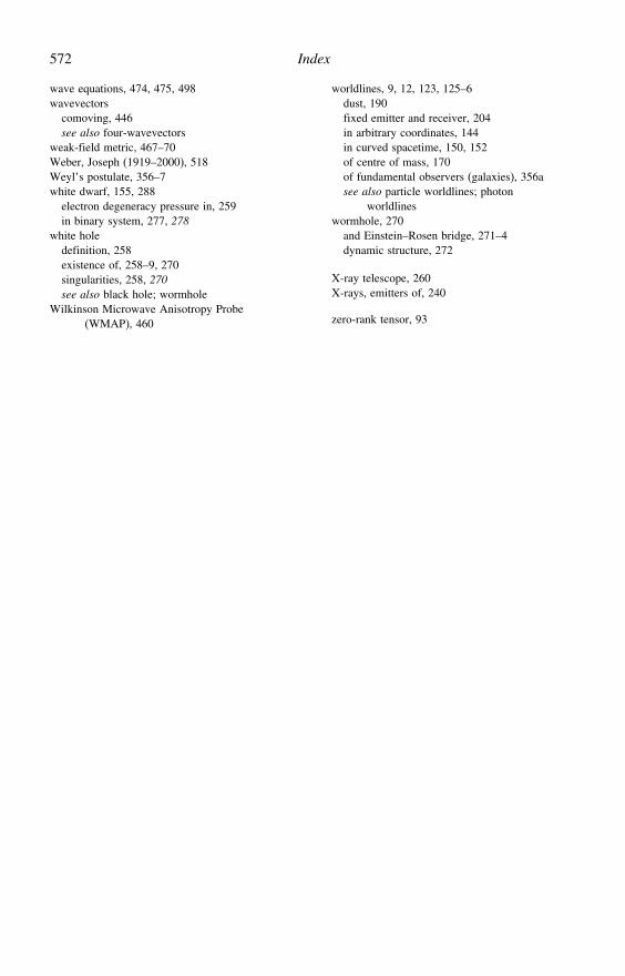
572 Index
wave equations, 474, 475, 498wavevectors
comoving, 446see also four-wavevectors
weak-field metric, 467–70Weber, Joseph (1919–2000), 518Weyl’s postulate, 356–7white dwarf, 155, 288
electron degeneracy pressure in, 259in binary system, 277, 278
white holedefinition, 258existence of, 258–9, 270singularities, 258, 270see also black hole; wormhole
Wilkinson Microwave Anisotropy Probe(WMAP), 460
worldlines, 9, 12, 123, 125–6dust, 190fixed emitter and receiver, 204in arbitrary coordinates, 144in curved spacetime, 150, 152of centre of mass, 170of fundamental observers (galaxies), 356asee also particle worldlines; photon
worldlineswormhole, 270
and Einstein–Rosen bridge, 271–4dynamic structure, 272
X-ray telescope, 260X-rays, emitters of, 240
zero-rank tensor, 93


