Probabilistic Engineering Mechanics 40 (2015) 25–35

Contents lists available at ScienceDirect

Probabilistic Engineering Mechanics

http://d0266-89

n CorrE-m

jimbeck

journal homepage: www.elsevier.com/locate/probengmech

General network reliability problem and its efficient solution by SubsetSimulation

Konstantin M. Zuev a,n, Stephen Wu b, James L. Beck b

a University of Liverpool, United Kingdomb California Institute of Technology, United States

a r t i c l e i n f o

Article history:Received 18 July 2014Received in revised form14 January 2015Accepted 2 February 2015Available online 4 February 2015

Keywords:Network reliabilityTechnological networksMarkov chain Monte CarloSubset SimulationSmall-world network models

x.doi.org/10.1016/j.probengmech.2015.02.00220/& 2015 Elsevier Ltd. All rights reserved.

esponding author.ail addresses: zuev@liverpool.ac.uk (K.M. Zuev@caltech.edu (J.L. Beck).

a b s t r a c t

Complex technological networks designed for distribution of some resource or commodity are a per-vasive feature of modern society. Moreover, the dependence of our society on modern technologicalnetworks constantly grows. As a result, there is an increasing demand for these networks to be highlyreliable in delivering their service. As a consequence, there is a pressing need for efficient computationalmethods that can quantitatively assess the reliability of technological networks to enhance their designand operation in the presence of uncertainty in their future demand, supply and capacity. In this paper,we propose a stochastic framework for quantitative assessment of the reliability of network service,formulate a general network reliability problem within this framework, and then show how to calculatethe service reliability using Subset Simulation, an efficient Markov chain Monte Carlo method that wasoriginally developed for estimating small failure probabilities of complex dynamic systems. The effi-ciency of the method is demonstrated with an illustrative example where two small-world networkgeneration models are compared in terms of the maximum-flow reliability of the networks that theyproduce.

& 2015 Elsevier Ltd. All rights reserved.

1. Introduction

Complex technological networks are a pervasive feature ofmodern society. The worldwide increase in urbanization and glo-balization, accompanied by rapid growth of infrastructure andtechnology, has produced complex networks with ever more in-terdependent components. These networks are designed for dis-tribution of some resource or commodity. Examples includetransportation networks (e.g. networks of roads or rail lines, ornetworks of airline routes), communication networks (e.g. tele-phone networks or the Internet), and utility networks (e.g. net-works for delivery of electricity, gas or water).

Technological networks are so deeply integrated into the in-frastructure of megacities that their failures, although rare, oftenhave serious consequences on the wellbeing of society. Societaldependence on technological systems and networks is constantlygrowing, giving an ever increasing vulnerability to their failure. Asa result, there is an increasing demand for modern technologicalnetworks to be highly reliable in their operations. The degree towhich a network is able to provide the required service needs to

), stewu@caltech.edu (S. Wu),

be quantitatively assessed during its design and operation, takinginto account uncertainty in the future demand, supply and net-work operational capacity.

Traditional methods for network reliability analyses are basedon graph theory and mostly look at small scale networks. Thesemethods aim to exactly compute the network reliability and canbe roughly classified by the following (not mutually exclusive)three categories: enumeration methods, direct methods, and de-composition methods. Enumeration methods are typically based oneither complete state enumeration or more sophisticated methodssuch as minpath or mincut enumeration, e.g. [1]. Direct methodsare intended to compute the reliability of a network from thestructure of the underlying graph, without a preliminary search forthe minpaths and mincuts, e.g. [13]. In decomposition methods, themain idea is to divide the network into several subnetworks, andthe overall reliability is then calculated based on the reliabilities ofthe corresponding subnetworks, e.g. [21]. A detailed review oftraditional methods for reliability analysis of small scale networksis provided in [15]. All these methods in one way or another arebased on combinatorial exhaustive search through the network.

On the other hand, one of the inherent characteristic features ofmodern technological networks is their very large size. Today thecomplexity of real-world networks can reach millions or evenbillions of vertices and edges with incomprehensible topology.Fig. 1 shows a visual representation of a small portion

Fig. 1. Man-made “galaxy”: a visual representation of a small portion ( 1%∼ ) of aCalifornia road network. Intersections and road endpoints are represented byvertices and the roads connecting these intersections or endpoints are representedby undirected edges. The network data is available for free at http://snap.stanford.edu/data/roadNet-CA.html. Visualization was done using the Network WorkbenchTool (available for free at http://nwb.slis.indiana.edu).

K.M. Zuev et al. / Probabilistic Engineering Mechanics 40 (2015) 25–3526

(approximately 1%) of a California road network. In this network,intersections and road endpoints are represented by vertices andthe roads connecting these intersections or endpoints are re-presented by undirected edges.

This dramatic change of scale induces a corresponding changein the philosophy of reliability analyses. Many of the exhaustivesearch algorithms that have been applied to small networks aresimply not feasible for large networks, since essentially all relia-bility problems of interest are NP-hard [27] and the exhaustivealgorithms grow in complexity very rapidly as a function of thenetwork size. It has been thus recognized that the classicalmethods of reliability and risk analysis fail to provide the properinstruments for analysis of actual modern networks [32]. As aresult, a new field of research has recently emerged with the focusshifting away from the combinatorial exhaustive search metho-dology to the study of statistical properties of large networks, to-gether with the study of their robustness to random failures, er-rors, and intentional attacks.

In this paper, we propose a stochastic framework for quanti-tative assessment of network reliability in the presence of un-certainty, formulate a general network reliability problem withinthis framework, and show how to solve this problem using SubsetSimulation [5], an efficient Markov chain Monte Carlo method thatwas originally developed for estimating small failure probabilitiesof complex dynamic systems, such as civil engineering structuresat risk from earthquakes. The new theory was first presented inthe conference paper [36] but here we give a fuller explanationand extended results. We remark that Subset Simulation has alsobeen used previously for evaluating origin–destination con-nectivity reliability of lifeline networks [9].

We proceed as follows. In the next section, we highlight thesimilarity between reliability problems for complex systems andcomplex networks, and formulate a general network reliabilityproblem subjected to several realistic conditions that make thisproblem computationally difficult. In Section 3, we describe the

Subset Simulation algorithm for solving the network reliabilityproblem. An illustrative example that demonstrates how SubsetSimulation can be effectively used for solving the maximum-flowreliability problem and for finding reliable network topologies isprovided in Section 4. Concluding remarks are made in Section 5.

2. From complex systems to complex networks

Complex networks are often viewed as the structural skeletonsof complex dynamic systems. While networks are a relatively newobject of study in reliability engineering, the reliability of dynamicsystems is a well-established and deeply researched problem. Theengineering research community has developed several very effi-cient methods for estimation of reliability of complex dynamicsystems such as tall buildings, bridges, and aircraft[4,5,18,7,8,16,34,35]. Moreover, it can be shown (see, e.g. [33]) thatthe system reliability problem is mathematically equivalent to twoother extensively researched problems: finding the free energy ofa physical system (statistical mechanics), and finding the marginallikelihood of a Bayesian statistical model (Bayesian statistics). Allthree problems can be considered as the problem of estimating theratio of normalizing constants for a pair of probabilitydistributions.

As a first step towards efficient network reliability methods,this paper focuses on the development of a network analog of thesystem reliability method, Subset Simulation [5]. In Section 2.1, webriefly review the system reliability problem to demonstrate itssimilarity with the network reliability problem which is discussedin Section 2.2.

2.1. System reliability problem

Calculation of the reliability, or equivalently the probability offailure pF, of a dynamic system under given excitation conditions isone of the most important and challenging problems in reliabilityengineering. The uncertainty in the input excitation x m∈ isquantified by a joint probability density function (PDF) x( )π . Theperformance of the dynamic system under this input is quantifiedby a performance function : mμ → through a dynamic input–output model of the system. For example, if our system corres-ponds to a tall building, the input x may represent an uncertainearthquake excitation sampled at discrete times over some inter-val and the performance x( )μ may represent the correspondingmaximum roof displacement over this duration, or the maximuminterstory drift over all stories for the duration, calculated from thedynamic model.

Define the failure domain F m⊂ as the set of inputs (“failurepoints”) that lead to the exceedance of some prescribed criticalthreshold μ ∈⁎ :

F x x{ ( ) } (1)m μ μ= ∈ | > ⁎

In the above example, the critical threshold μ⁎ represents themaximum permissible roof displacement or maximum permis-sible interstory drift and so the failure domain F represents the setof all earthquake excitations that lead to unacceptable deforma-tion of the tall building.

The system reliability problem is then to compute the prob-ability of failure that is given by the following integral:

p x F x dx x I x dx I( ) ( ) ( ) ( ) [ ], (2)F FF Fm∫ ∫π π= ∈ = = = π

where π denotes expectation with respect to the distribution x( )πand IF is the indicator function of the failure domain F: I x( ) 1F = ifthe system subject to excitation x fails (i.e. the output x( )μ is notacceptable according to the performance criterion, x( )μ μ> ⁎) and

K.M. Zuev et al. / Probabilistic Engineering Mechanics 40 (2015) 25–35 27

I x( ) 0F = otherwise.The following set of realistic assumptions makes this problem

computationally very challenging:

S1.

The relationship between x and IF(x) is not explicitly known. Al-though for any x we can check whether it is a failure point ornot by numerical analysis using a model of the dynamic sys-tem, i.e. calculate the value IF(x) for a given x, we cannotusually obtain an explicit analytical formula for x( )μ or itsgradient with respect to x.

S2.

The computational effort for the dynamic system analysis neededto evaluate x( )μ for each value of x is significant so that it isessential to minimize the number of such function evaluations.Complex dynamic systems (e.g. bridges or aircraft) are re-presented by complex models. In this context, complexitymeans, in particular, that the evaluation of x( )μ for any x isvery time-consuming. Thus, it is important to reduce thenumber of such function evaluations.

S3.

The dimension m is large, i.e. m 1⪢ , because the stochastic inputtime history is discretized in time. For example, m∼103 is notunusual in the reliability literature.

S4.

The probability of failure pF is very small, i.e. p 1F ⪡ . In otherwords, the system is assumed to be designed properly, so thatfailure is a rare event. In the reliability engineering literature,p 10 10F

9 2∼ –− − have been considered.

Fig. 2. The undirected graph on the top is equivalent to the directed graph at thebottom. Both graphs are described by the adjacency matrix A.

Due to these conditions, both numerical integration and standardMonte Carlo are computationally infeasible for estimating thehigh-dimensional integral in (2).

Over the past decade, the engineering research community hasrealized the importance of advanced stochastic simulation meth-ods for reliability analysis. As a result, many efficient algorithmshave been recently developed, e.g. Subset Simulation by Au andBeck [5], Line Sampling by Koutsourelakis et al. [18], AuxiliaryDomain method by Katafygiotis et al. [16], Horseracing Simulationby Zuev and Katafygiotis [34], Bayesian Subset Simulation by Zuevet al. [35], to name but a few.

Since complex networks can be viewed as the structural ske-letons of complex systems, it is natural to expect that the abovetechniques can be adapted for efficient estimation of networkreliability.

2.2. Network reliability problem

A network topology is represented as a graph G V E( , )= , whereV v v{ , , }n1= … and E e e{ , , }m1= … are sets of n nodes (or vertices)and m links (or edges), respectively. Any graph G with n nodes canbe represented by its n�n adjacency matrix A(G), where A 1ij = ifthere is a link directly connecting vi to vj (i j≠ ) and A 0ij =otherwise. The degree of a node v Vi ∈ , denoted d v( )i , is thenumber of links incident to the node and it is equal to the ith rowsum of A. The graph G may be either undirected or directed. In thelatter case, the adjacency matrix A(G) is not necessarily symmetric.In this case, node degree d(v) is replaced by in-degree din(v) andout-degree dout(v), which count the number of links pointing intowards, and out from, a node, respectively. In general, any un-directed network can be considered as directed after replacementof every undirected link by two corresponding opposing directedlinks. The concept of adjacency matrix and the equivalence ofundirected graphs to directed ones are demonstrated in Fig. 2.

In what follows we assume that nodes are perfectly reliable, i.e.they have zero failure probability. It can be shown that any net-work with node failures is polynomial-time reducible into anequivalent directed network with link failures only [10]. Thus, thisassumption does not, in fact, limit the generality, and networkswith link failures only are sufficiently general.

A network state is defined as an m-tuple s s s( , , )m1= … withs [0, 1]i ∈ , where si¼1 if link ei is fully operational (or “up”) andsi¼0 if link ei is completely failed (or “down”). If s (0, 1)i ∈ , thenlink ei is partially operational. The network state space is then anm-dimensional hypercube:

{ }s s s( , , ) [0, 1] [0, 1] (3)m im

1= … | ∈ =

Let s( )π be a probability distribution on the network state spacewhich provides a probability model for the occurrence of dif-

ferent network states. We write s s( )π∼ . For example, if we as-sume that each link ei is either up (si¼1) or down (si¼0) and thatlinks fail independently of each other with failure probabilities pi,then this induces a discrete probability distribution s( )π on : eachstate s s s( , , )m1= … with s 0, 1i = has occurrence probability

s q p( ) ,(4)i

m

is

is

1

1i i∏π ==

−

where q p1i i= − is the link reliability; partially operational linksdo not occur in this case.

In this work, we focus on the more general case of continuousstate spaces where s( )π denotes a PDF on . Furthermore, wedefine a performance function :μ → that quantifies the degreeto which the network provides the required service. In the contextof networks, μ is typically interpreted as a utility function, i.e.higher values of μ correspond to better network performance.Similar to the system case (1), the failure domain ⊂ is definedas follows:

Table 1Notation.

G V E( , )= Graph representing a network

V v v{ , , }n1= … Set of nodes (or vertices)

E e e{ , , }m1= … Set of links (or edges)

A(G) Adjacency matrix of Gd v d v d v( ), ( ), ( )in out Degree, in-degree, and out-degree of node v

s s s( , , )m1= … A network state, where s [0, 1]i ∈ , i¼1,…,m

[0, 1]m= Network state space (set of all network states)

s( )π Probability distribution on:μ → Network performance function

⊂ Failure domain

K.M. Zuev et al. / Probabilistic Engineering Mechanics 40 (2015) 25–3528

s s{ ( ) }, (5)μ μ= ∈ | < ⁎

where μ⁎ is the critical threshold. The notation is summarized inTable 1.

The network reliability problem is to compute the probability offailure p that is given by the following integral:

p s s I s ds I( ) ( ) ( ) [ ]. (6)∫ π= ∈ = = π

Several classical reliability problems [6,27,10] are special casesof the above general formulation, e.g. Source-to-Terminal Con-nectedness, Network Connectedness, Traffic to Central Site, toname but a few.

To mirror the systems framework S1–S4, we make the follow-ing real-life assumptions:

N1.

The relationship between s ∈ and I s( ) is not explicitly known. N2. The computational effort for evaluating the network performance

function s( )μ for each state s ∈ is significant, thereby makingthe indicator function I s( ) expensive to compute. Therefore, itis essential to minimize the number of such functionevaluations.

N3.

The number of links m is large, i.e. m 1⪢ . Many actual networkshave millions (e.g. road networks), or even billions, of links(e.g. the Internet).

N4.

The probability of failure p is very small, i.e. p 1⪡ . Real-lifenetworks are reliable to some extent (otherwise they wouldnot be in use), and their failures are usually rare events.

Fig. 3. A schematic representation of the intermediate failure domainsL0 1= ⊃ ⊃ ⋯ ⊃ = in the network state space [0, 1]m= , where m¼2.

These assumptions make the network reliability problemcomputationally very challenging. Due to N3, the integral in (6) istaken over a high-dimensional hypercube and, due to N2, the in-tegrand is expensive to compute. Therefore, the exact computationof the failure probability p is infeasible.

The expression of p as a mathematical expectation (6) rendersstandard Monte Carlo method theoretically applicable, where p isestimated as a sample average of I s( ) over independent andidentically distributed samples of s drawn from distribution s( )π :

pN

I s s s1

( ), ( )(7)

MC

i

Ni i( )

1

( ) ( )∑ π^ = ∼=

This estimate is unbiased and the coefficient of variation, servingas a measure of the statistical error, is

p

Np

1

(8)MCδ =

−

Although standard Monte Carlo is independent of the dimensionm of the network state space , it is inefficient in estimating smallprobabilities because it requires a large number of samples( p1/∼ ) to achieve an acceptable level of accuracy. For example, if

p 10 4= − and we want to achieve an accuracy of 10%MCδ = , then

we need approximately N 106= samples. Therefore, due to con-ditions N2 and N4, standard Monte Carlo becomes computation-ally prohibitive for our problems of interest involving small failureprobabilities.

The basic strategy that is often employed in this situation is togenerate more samples in the “important region” of the failure

domain, i.e. in the region ′ ⊆ that contains most of the prob-ability mass and, therefore, contributes mostly to the integral (6).

More formally, we want to sample from distribution s( )ψ on ′,where s( )ψ is the conditional distribution s s( ) ( )ψ π= | ′ or, possi-bly, some other importance sampling distribution with support

ssupp ( )ψ = ′. To achieve this goal, we can use Markov chainMonte Carlo (MCMC) methods, a class of algorithms for samplingfrom complex probability distributions. In MCMC, samples from agiven (up to a normalizing constant) distribution s( )ψ are gener-ated by simulating a Markov chain whose state distribution con-verges to the target distribution s( )ψ as its stationary distribution.Markov chain Monte Carlo sampling originated in statistical phy-sics, and now is widely used in solving statistical problems [20,26].In the next section we show how MCMC can be employed forsolving the network reliability problem.

3. Subset Simulation

The main idea of Subset Simulation [5] is to represent a smallfailure probability p as a product p pj

Lj1= ∏ = of larger prob-

abilities p pj > , where the factors pj are estimated sequentially,

p pj j≈ ^ to obtain an estimate p̂ for p as p pjL

j1^ = ∏ ^

= . Toachieve this goal, let us consider a sequence of nested subsets ofthe network state space , starting from the entire space andshrinking to the failure domain:

(9)L0 1= ⊃ ⊃ ⋯ ⊃ =

Subsets , , L0 1… − are called intermediate failure domains. Theyare schematically shown in Fig. 3. The failure probability can bewritten then as a product of conditional probabilities:

K.M. Zuev et al. / Probabilistic Engineering Mechanics 40 (2015) 25–35 29

p p( ) ,(10)j

L

j jj

L

j1

11

∏ ∏= | ==

−=

where p ( )j j j 1= | − is the conditional probability at the ( j 1− )thconditional level. Clearly, by choosing the intermediate failuredomains , , L1 1… − appropriately, all conditional probabilitiesp p, , L1 … can be made sufficiently large. The original network re-liability problem (estimation of the small failure probability p ) isthus replaced by a sequence of L intermediate problems: estima-tion of the larger failure probabilities pj, j¼1,…,L.

The first probability p ( ) ( )1 1 1= | = can be simply esti-mated by standard Monte Carlo simulation (MCS):

p pN

I s s s s1

( ), ( ) ( )(11)i

Ni i i i d

1 11

0( )

0( ) . . .

01∑ π π≈ ^ = ∼ | ≡=

We assume here that 1 is chosen in such a way that p1 is relativelylarge, so that the MCS estimate (11) is accurate for a moderatesample size N. Later in this section, we will discuss how to choseintermediate failure domains j adaptively.

For j 2≥ , to estimate pj using MCS one needs to simulate i.i.d.samples from the conditional distribution s( )j 1π | − , which, for general

s( )π and j 1− , is not a trivial task. For example, it would be inefficientto use MCS for this purpose (i.e. to sample from s( )π and accept onlythose samples that belong to j 1− ), especially at higher levels. Sam-pling from s( )j 1π | − for j 2≥ can be done by a specifically tailoredMCMC technique at the expense of generating dependent samples.

The Metropolis–Hastings (MH) algorithm [22,14] is perhaps themost popular MCMC algorithm for sampling from a probabilitydistribution that is difficult to sample from directly. In this algo-rithm, samples are generated as the states of a Markov chain,which has the target distribution, i.e. the distribution we want tosample from, as its stationary distribution. In our case, the targetdistribution is s s I s( ) ( ) ( )/j j1 1j 1π π| =− −− , where ( )j j1 1=− − is

a normalizing constant. Let s ji

1( )

− be the current state of the Markov

chain at level (j�1) and q s s( )ji

1( )| − , called the proposal PDF, be anm-

dimensional PDF on the network state space that may dependon s j

i1

( )− and can be readily sampled. Then the MH update

s sji

ji

1( )

1( 1)→− −

+ of the Markov chain works as follows:

1.

Generate a candidate state ξ ∈ according to q s s( )ji

1( )| − .

2.

Compute the acceptance probability I ( ) minj 1α ξ= −

{ }q s s q s1, ( ) ( )/ ( ) ( )ji

ji

ji

1( )

1( )

1( )π ξ ξ π ξ| |− − − .

Sub

In

▹▹

Al

3. Accept ξ as the next state of the Markov chain, i.e. set s ji

1( 1) ξ=−

+ ,

with probability α, or reject it, i.e. set s sji

ji

1( 1)

1( )=−

+− with the

remaining probability 1 α− .

It is easy to show that this update leaves s( )j 1π | − invariant, i.e. ifs j

i1

( )− is distributed according to s( )j 1π | − , then so is s j

i1

( 1)−+ , and if

the Markov chain is run for sufficiently long time (the “burn-inperiod”), starting from essentially any “seed” s j j1

(1)1∈− − , then for

large N the distribution of s jN

1( )

− will be approximately s( )j 1π | − .Note, however, that usually it is very difficult to check whether theMarkov chain has converged to its stationary distribution. But ifthe seed s s( )j j1

(1)1π∼ |− − , then all states of the Markov chain will

be automatically distributed according to the target distribution,s s i N( ), 1, ,j

ij1

( )1π∼ | = …− − . The absence of the burn-in period (i.e.

the absence of the convergence problem) is often referred to asperfect sampling [26] and Subset Simulation has this propertybecause of the way the seeds are selected.

It was observed in [5] however that the original Metropolis–Hastings algorithm suffers from the curse of dimensionality.Namely, it is not efficient in high-dimensional conditional prob-ability spaces, because it produces a Markov chain with veryhighly correlated states. Therefore, if the total number of networklinks m is large, then the MH algorithm will be inefficient forsampling from s( )j 1π | − , where [0, 1]j

m1 ⊂ =− . In Subset Si-

mulation, the Modified Metropolis algorithm (MMA) [5], a com-ponent-wise MCMC technique based on the original MH algo-rithm, is used instead for sampling from the conditional dis-tributions s( )j 1π | − . MMA differs from the MH algorithm in theway the candidate state ( , , )m1ξ ξ ξ= … is generated. Instead ofusing an m-dimensional proposal PDF on to directly obtain thecandidate state, in MMA a sequence of univariate proposal PDFs isused. Namely, each component ξk of the candidate state vector ξ isgenerated separately using a univariate proposal distributionq s s( )k k j k

i1,

( )| − dependent on the kth component s j ki

1,( )

− of the cur-

rent state sample s ji

1( )

− . Then a check is made whether the m-variate candidate ξ ∈ generated in such a way belongs to thesubset j 1− in which case it is accepted as the next Markov chainstate; otherwise it is rejected and the current MCMC sample isrepeated. For details on MMA, we refer the reader to the originalpaper [5] and to [35] where the algorithm is discussed in depth.

Let us assume now that we are given a seed s s( )j j1(1)

1π∼ |− − ,where j¼2,…,L. Then, using MMA, we can generate a Markov chainwith N states starting from this seed and construct an estimate for pjsimilar to (11), where MCS samples are replaced by MCMC samples:

p pN

I s s s1

( ), ( )(12)

j ji

N

ji

ji MMA

j1

1( )

1( )

1j∑ π≈ ^ = ∼ |=

− − −

Note that all samples s s, ,j jN

1(1)

1( )…− − in (12) are identically distrib-

uted in the stationary state of the Markov chain, but are notindependent. Nevertheless, these MCMC samples can be used forstatistical averaging as if they were i.i.d., although with somereduction in efficiency [11].

Subset Simulation uses the estimates (11) for p1 and (12) for pj,j 2≥ , to obtain the estimate for the failure probability:

p p p(13)j

L

j1

∏≈ ^ = ^=

The remaining ingredient of Subset Simulation that we have todiscuss is the choice of intermediate failure domains , , L1 1… − .Recall that the “ultimate” failure domain L= ∈ is defined as

s s{ ( ) }μ μ= ∈ | < ⁎ . The sequence of intermediate failure do-mains can then be defined in a similar way:

s s{ ( ) }, (14)j jμ μ= ∈ | < ⁎

where L L 1 1μ μ μ μ= < < ⋯ <⁎ ⁎−

⁎ ⁎ is a sequence of intermediatecritical thresholds. Intermediate threshold values jμ ⁎ define the

values of the conditional probabilities p ( )j j j 1= | − and, there-fore, affect the efficiency of Subset Simulation. In practical cases itis difficult to make a rational choice of the valuesjμ −⁎ in advance,so the jμ ⁎ are chosen adaptively (see (15) below) so that theestimated conditional probabilities are equal to a fixed valuep (0, 1)0 ∈ . In [35], p0 is called the conditional failure probability.

S

set Simulation algorithm for network reliability problem.

put:p0, conditional failure probability;N, number of samples per conditional level.gorithm:et j¼0, number of conditional level

S

Sf

ew

eOu

K.M. Zuev et al. / Probabilistic Engineering Mechanics 40 (2015) 25–3530

et N j( ) 0= , number of failure samples at level j

ample s s s, , ( )N i i d0(1)

0( ) . . . π… ∼

or i¼1,…,N do

if s( )i i( )0( )μ μ μ= < ⁎ do

N j N j( ) ( ) 1← +end ifnd forhile N j Np( ) 0< do

j j 1← +

Sort { }i( )μ : i i i( ) ( ) ( )N1 2μ μ μ≤ ≤ ⋯ ≤Define the jth intermediate critical threshold:

2 (15)j

i i( ) ( )Np Np0 0 1μ μ μ= +⁎

+

for k Np1, , 0= … do

Starting from s s s( )jk

ji

j(1),

1( )k π= ∼ |− , generate p1/ 0 states

of a Markov chain s s s, , ( )jk

jp k

j(1), (1/ ),0 π… ∼ | , using

MMA.end for

Renumber: s s s s{ } , , ( )ji k

k iNp p

j jN

j( ),

1, 1,1/ (1) ( )0 0 π↦ … ∼ |= =

for i¼1,…,N do

if s( )iji( ) ( )μ μ μ= < ⁎ do

N j N j( ) ( ) 1← +end if

end fornd whiletput:

p̂ , estimate of p :

▶

p pN j

N( )

(16)j

0^ =

The adaptive choice of valuesjμ −⁎ in (15) guarantees, first, that

all seeds s jk(1), are distributed according to s( )jπ | and, second, that

the estimated conditional probability ( )j j 1| − is equal to p0.Here, for convenience, p0 is assumed to be chosen such that Np0and p1/ 0 are positive integers, although this is not strictly neces-sary. It was demonstrated in [35] that choosing any p [0.1, 0.3]0 ∈will lead to similar efficiency and it is not necessary to fine tunethe value of the conditional failure probability as long as SubsetSimulation is implemented properly.

4. Illustrative example: maximum flows in small-worldnetworks

In this section, we demonstrate how Subset Simulation can beused for efficient solution of the maximum-flow reliability problemfor networks generated from small-world models.

4.1. The maximum-flow reliability problem

Network flow problems naturally arise in many real world appli-cations such as coordination of vehicles in a transportation network,distribution of water in a utility network, and routing of packets in acommunication network. The maximum-flow problem, where thegoal is to maximize the total flow from one node of a network toanother, is one of the classical network flow problems [12].

Suppose that in addition to a network G V E( , )= , a dis-tinguished pair of nodes, the source a V∈ and the sink b V∈ , isspecified. Also assume that each link e v u E( , )= ∈ has a non-ne-gative flow capacity s v u( , ) 0≥ . A quadruple G a b s( , , , { }) is oftenreferred to as a flow network. A flow on G is non-negative function

f E: → + that satisfies the following properties:

�

Capacity constraint: the flow along any link cannot exceedthe capacity of that link:

f v u s v u v u E( , ) ( , ) for all ( , ) (17)≤ ∈

Flow conservation: the total flow entering node v must equal

� the total flow leaving v for all nodes except a and b:

f u v f v u v V a b( , ) ( , ) for all \{ , }(18)u V u V

∑ ∑= ∈∈ ∈

For convenience, it is assumed in (18) that f v u( , ) 0= ifv u E( , ) ∉ (no link from node v to node u).

The value f| | of a flow f is the net flow out of the source:

f f a v f v a( , ) ( , )(19)v V v V

∑ ∑| | = −∈ ∈

It is easy to show that f| | also equals the net flow into the sink:

f f v b f b v( , ) ( , )(20)v V v V

∑ ∑| | = −∈ ∈

The value of a flow represents how much one can transport fromthe source to the sink.

The maximum-flow problem is that of finding the maximumflow f farg max= | |⋆ over all possible flows f in a given flow net-work G a b s( , , , { }). There is a simple algorithm called the aug-mented path algorithm (also called the Ford–Fulkerson algorithm)that calculates the maximum flows between nodes in polynomialtime. The theory of maximum flow algorithms is well covered in[2].

The maximum-flow reliability problem considered in this paperis motivated by the maximum-flow problem. Assume for con-venience that all link capacities s s, , m1 … are normalized, s0 1i≤ ≤ ,and suppose that, instead of being prescribed, they are uncertainwith their uncertainty quantified by a probability model π for alllink capacities, i.e. a probability distribution on the network statespace s s s s{ ( , , ) 0 1}m i1= = … | ≤ ≤ . For a given realizations s( )π∼ , we define the max-flow network performance function tobe equal to the value of the corresponding maximum flow:

s f s( ) ( ) (21)MFμ = | |⋆

The failure domain ⊂ can now be defined as before,s s{ ( ) }MFμ μ= ∈ | < ⁎ , where μ⁎ is the critical threshold. Thus, the

introduction of uncertain link capacities brings us into the generalnetwork reliability framework described in Section 2.2.

One of the fundamental questions in network science and re-liability theory is the following: given n nodes and m links, howshould they be combined into the most reliable network? This is acomputationally challenging optimization problem. In the nextsection we analyze a simpler but related question: given twonetwork models that generate componentwise equivalent but to-pologically different networks, how do we find out which networkmodel produces more reliable networks?

4.2. Small-world network models

One of the most important breakthroughs in modeling real-world networks was a shift from classical random graph models,where links between nodes are placed purely at random, to

K.M. Zuev et al. / Probabilistic Engineering Mechanics 40 (2015) 25–35 31

models that explicitly mimic certain statistical properties observedin actual networks. Small-world network models were originallyinspired by the counter intuitive phenomenon observed by thesocial psychologist Stanley Milgram in human social networks[23]. In his famous experiment, each of the participants (randomlychosen in Nebraska) was asked to forward a letter to one of theirfriends in an attempt to get the letter ultimately to a desired targetperson (who lived in Boston, Massachusetts). The obtained resultswere very surprising: the average number of people needed totransmit the letter to the target was approximately six. This gavebirth to the popular belief that there are only about six handshakesbetween any two people in the world, so-called “six degrees ofseparation”. Milgram's experiment was one of the first quantita-tive observations of the small-world effect, the fact that despitetheir often large size and high level of clustering, in most actualnetworks there is a relatively short path between almost any twonodes. The small-world effect has been observed in many realnetworks [30,24], including technological ones such as powergrids [31], airline routes [3], and railways [28].

In their seminal paper [31], Watts and Strogatz proposed thefirst network model (the WS model) that generates “small-worlds”, i.e. networks with small average shortest-path lengthsand high levels of clustering. The original WS model is a one-parameter model which interpolates between a regular lattice anda random graph. The model starts from a one-dimensional latticeof n nodes with periodic boundary conditions, i.e. a ring lattice.Each node is then connected to its first k2 neighbors (k on eitherside), with k n⪡ . Thus we obtain a regular symmetric lattice withm¼nk links. The small-world network is then created by takingeach link in turn and, with probability p, rewiring one end of thatlink to a new node chosen uniformly at random. The rewiringprocess generates on average pnk long-range connections. Notethat, as p goes from 0 to 1, the model moves from a deterministicregular lattice to a random graph. For p0 1< < , the WS modelgenerates networks with the small-world property.

Since the pioneering work of Watts and Strogatz, many mod-ifications of the WS model have been proposed and studied. Other

Fig. 4. Road networks in (a) Beijing, China and (b) Los Angeles, USA. Both plots are obtmodel (like Fig. 5(a)) and the torus model (like Fig. 5(b)), respectively.

small-world network models that have become popular includethe Newman–Watts model [25], where, instead of rewiring links,new links connecting randomly chosen pairs of nodes are added,and the Kleinberg model [17], where small-world networks arebuilt on a d-dimensional lattice and the probability that two nodesare connected by a long-range link depends on the distance be-tween them in the lattice. In general, small-world models can beconstructed on lattices of any dimension and any topology. For astate-of-the-art review of the subject, we refer the reader to [24].

In this paper, we consider two small-world network modelsthat are built on one- and two-dimensional lattices with periodicboundary conditions, the small-world ring model and the small-world torus model, respectively.

�

aine

Small-world ring model n k( , )⊗ : As with the WS model, n k( , )⊗starts with a ring lattice of n nodes. This lattice has n un-directed links, which equivalently can be considered as n2 di-rected links (recall Fig. 2). Next, for each node v, the modelgenerates k additional directed links connecting that node withk other nodes v v, , k1 … chosen uniformly at random. Note thatfor each selected vi, either link v v( , )i or v v( , )i is constructedwith equal probabilities.

�

Small-world torus model n k( , )⊠ : This model starts with asquare n�n lattice. Periodic boundary conditions make it to-pologically equivalent to a 2-D torus, hence the name of themodel. This torus has 2n2 undirected links, or, equivalently, 4n2

directed links. The small-world torus n k( , )⊠ is then created byadding k directed links per each node in the same way as in thecase of n k( , )⊗ above.

Small-world network models are often used to study practicalproblems in various fields, such as transportation, biology, andsocial science [19]. For example, [29] reviews recent research thathas been done in social science and management using small-world networks. Another important application is the reliabilitystudy of transportation networks. The development of a trans-portation network usually starts with a fixed plan to connect some

d from Google Maps. The Beijing and LA networks can be modeled by the ring

Fig. 5. (a) Realization of the small-world ring model n k( , )⊗ , with n¼16 and k¼3. Solid and dashed lines represent regular links and random shortcuts, respectively. Forvisibility, only random shortcuts that correspond to nodes 1, 5, 9, and 13 are shown. (b) Realization of the small-world torus model n k( , )⊠ , with n¼4 and k¼1. Solid anddashed lines represent regular links and random shortcuts, respectively. For visibility, only random shortcuts that correspond to nodes 1, 4, 13, and 16 are shown.

K.M. Zuev et al. / Probabilistic Engineering Mechanics 40 (2015) 25–3532

regions in a city, and then more roads are built as the city growsand the demand of roads increases. The small-world network re-sembles this process very well. The similarity between realtransportation networks and synthetic realizations of small-worldmodels can often be visually observed. For example, Fig. 4(a) shows part of the transportation network in Beijing, China, thatcan be represented by the small-world ring model; Fig. 4(b) showspart of the transportation network in Los Angeles, USA, that can berepresented by the small-world torus model.

Hereafter, we refer to deterministic lattice links as the regularlinks and to the randomly generated links as the random shortcuts.Realizations of (16, 3)⊗ and (4, 1)⊠ are schematically shown inFig. 5(a) and (b), respectively.

In Table 2, the total number of network components is pro-vided for both models. It is easy to see that n k( , )1 1⊗ and n k( , )2 2⊠produce componentwise equivalent networks if and only if n n1 2

2=and k k 21 2= + . Topologically, however, the network realizations ofthese models will still be different, since the underlying latticeshave different dimensions. Thus, we have

n k n k

n k n k

Componentwise: ( , 2) ( , )

Topologically: ( , 2) ( , ) (22)

2

2

⊗ + = ⊠

⊗ + ≠ ⊠

The small-world torus model n k( , )⊠ has more regular links,while the small-world ring model n k( , 2)2⊗ + has more randomshortcuts. This split between the number of regular links versusrandom shortcuts, which represents the tradeoff between local

Table 2Componentwise comparison of two small-world models, n k( , )⊗ and n k( , )⊠ .

Model # of nodes # of regularlinks

# of randomshortcuts

Total # of links

n k( , )⊗ n n2 kn n k( 2)+n k( , )⊠ n2 4n2 kn2 n k( 4)2 +

connectivity and global reachability, has the potential to yieldsignificantly different reliability properties for the two networkmodels. Fig. 6(a) and (b) shows an example for both models whenn is large. To demonstrate the effectiveness of Subset Simulationfor network reliability estimation, we investigate the followingquestion: Which model, n k( , 2)2⊗ + or n k( , )⊠ , produces morereliable networks where reliability is understood as the max-imum-flow reliability?

4.3. Simulation results

Reliabilities of two network models with different topologiescan be compared in the following way. Given a network realization

n k( , 2)2⊗̂ ∼ ⊗ + , a source–sink pair (a,b), and the criticalthreshold μ⁎, we can estimate the network failure probability

p a b( ; ( , ); )μ⊗̂ ⁎ with respect to the max-flow performancefunction (21), using Subset Simulation described in Section 3. Byaveraging over different network realizations and source–sinkpairs, we obtain the expected failure probability for a given criticalthreshold for the small-world ring model:

p p a b

Mp a b

( ) [ ( ; ( , ); )]

1( ; ( , ); )

(23)

a b

i

M

i i i

, ,( , )

1

∑

μ μ

μ

¯ = ⊗̂

≈ ⊗̂

⊗⁎

⊗⁎

=

⁎

Similarly we can estimate the expected failure probability for thesmall-world torus model:

p p a b

Mp a b

( ) [ ( ; ( , ); )]

1( ; ( , ); ),

(24)

a b

i

M

i i i

, ,( , )

1

∑

μ μ

μ

¯ = ⊠̂

≈ ⊠̂

⊠⁎

⊠⁎

=

⁎

where n k( , )i⊠̂ ∼ ⊠ are i.i.d, and node pairs a b( , )i i are chosenuniformly at random.

Fig. 6. (a) Realization of the small-world ring model n k( , 2)2⊗ + , with n¼40 and k¼2. (b) Realization of the small-world torus model n k( , )⊠ , with n¼40 and k¼2.

K.M. Zuev et al. / Probabilistic Engineering Mechanics 40 (2015) 25–35 33

Since our goal is to compare reliabilities of networks that areproduced by the two network models, we are interested not in thefunctions p ( ), μ¯ ⊗

⁎ and p ( ), μ¯ ⊠⁎ per se, but rather in their relative

behavior. We can achieve this by treating the critical threshold μ⁎

as a parameter and plotting p ,¯ ⊗ versus p ,¯ ⊠. The resulting curvewill lie in the unit square, since both probabilities are between0 and 1; it starts at (0, 0), since both probabilities converge to 0, asμ → − ∞⁎ ; and it ends at (1, 1), since both probabilities converge to1, as μ → + ∞⁎ . We refer to this curve as the relative reliabilitycurve. We are especially interested in the behavior of the relativefailure probability curve in the vicinity of the origin (0, 0), sincethis region corresponds to highly reliable networks, and an accu-rate estimation of failure probabilities in this region is especiallychallenging.

In this paper, we compare the reliability properties ofn k( , 2)2⊗ + and n k( , )⊠ for two values of n, namely, n¼5 and

n¼8. For each n, we consider several values of k, i.e. several dif-ferent numbers of random shortcuts per node. The number of

0 0.2 0.4 0.6 0.8 10

0.2

0.4

0.6

0.8

1

p1

p 2

Relative Reliability Curve (Linear Scale)

k =0k =1k =2k =3

n=5

Fig. 7. The relative reliability curve in the linear scale (left panel) and log scale (right p

samples used in each Subset Simulation run is N¼2000 per level,and the conditional failure probability is p0¼0.1. Figs. 7 and 8show the resulting relative reliability curves for n¼5 and n¼8,respectively.

For n¼5, k 0, 1, 2,= and 3 are studied. For both small-worldring and small-world torus models, M¼200 network realizations{ }i⊗̂ and { }i⊠̂ and source–sink pairs a b{( , )}i i are generated toestimate the expected failure probabilities in (23) and (24). A finegrid of valuesμ −⁎ between 0.1 and 3 is used to obtain the relativereliability curve in Fig. 7. For n¼8, k 0, 1, 2,= and 4 are con-sidered. In this case, M¼100 network realizations and source–sinkpairs are simulated to estimate p ( ), μ¯ ⊗

⁎ and p ( ), μ¯ ⊠⁎ in (23) and

(24), respectively. A fine grid of valuesμ −⁎ between 0.1 and 6 isused to obtain the relative reliability curve in Fig. 8.

For both n¼5 and n¼8, we observe the following results:

1.

10

10

10

1

p 2

anel

The relative reliability curve lies below the equal reliabilityline, i.e. below the diagonal that connects the origin (0, 0)

10−6 10−4 10−2 100

−6

−4

−2

00

p1

Relative Reliability Curve (Log Scale)

k =0k =1k =2k =3

n=5

), for n¼5. Here, p p1 ,= ¯ ⊗ and p p2 ,= ¯ ⊠ as in (23) and (24) for (0.1, 3)μ ∈⁎ .

0 0.2 0.4 0.6 0.8 10

0.2

0.4

0.6

0.8

1

p1

p 2

Relative Reliability Curve (Linear Scale)

10010−210−410−610−8

10−8

10−6

10−4

10−2

100

p1

p 2

Relative Reliability Curve (Log Scale)

k =0k =1k =2k =4

k =0k =1k =2k =4

n=8 n=8

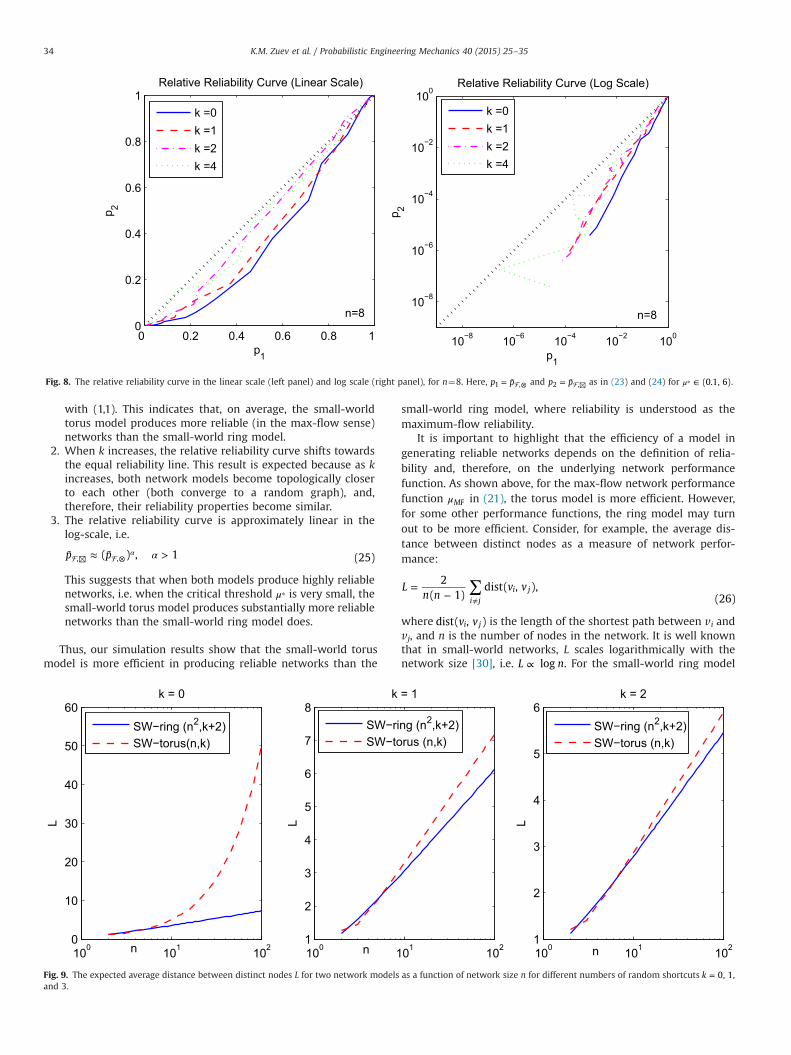
Fig. 8. The relative reliability curve in the linear scale (left panel) and log scale (right panel), for n¼8. Here, p p1 ,= ¯ ⊗ and p p2 ,= ¯ ⊠ as in (23) and (24) for (0.1, 6)μ ∈⁎ .

L

Fig. 9and

K.M. Zuev et al. / Probabilistic Engineering Mechanics 40 (2015) 25–3534

with (1,1). This indicates that, on average, the small-worldtorus model produces more reliable (in the max-flow sense)networks than the small-world ring model.

2.

When k increases, the relative reliability curve shifts towardsthe equal reliability line. This result is expected because as kincreases, both network models become topologically closerto each other (both converge to a random graph), and,therefore, their reliability properties become similar.

3.

The relative reliability curve is approximately linear in thelog-scale, i.e.

p p( ) , 1 (25), , α¯ ≈ ¯ >α⊠ ⊗

This suggests that when both models produce highly reliablenetworks, i.e. when the critical threshold μ⁎ is very small, thesmall-world torus model produces substantially more reliablenetworks than the small-world ring model does.

Thus, our simulation results show that the small-world torusmodel is more efficient in producing reliable networks than the

100 101 1020

10

20

30

40

50

60

n

k = 0

SW−ring (n2,k+2)SW−torus(n,k)

100 11

2

3

4

5

6

7

8

n

L

k

SW−riSW−to

. The expected average distance between distinct nodes L for two network models3.

small-world ring model, where reliability is understood as themaximum-flow reliability.

It is important to highlight that the efficiency of a model ingenerating reliable networks depends on the definition of relia-bility and, therefore, on the underlying network performancefunction. As shown above, for the max-flow network performancefunction MFμ in (21), the torus model is more efficient. However,for some other performance functions, the ring model may turnout to be more efficient. Consider, for example, the average dis-tance between distinct nodes as a measure of network perfor-mance:

Ln n

v v2

( 1)dist( , ),

(26)i ji j∑=

− ≠

where v vdist( , )i j is the length of the shortest path between vi andvj, and n is the number of nodes in the network. It is well knownthat in small-world networks, L scales logarithmically with thenetwork size [30], i.e. L nlog∝ . For the small-world ring model

01 102

= 1

ng (n2,k+2)rus (n,k)

100 101 1021

2

3

4

5

6

n

L

k = 2

SW−ring (n2,k+2)SW−torus (n,k)

as a function of network size n for different numbers of random shortcuts k 0, 1,=

K.M. Zuev et al. / Probabilistic Engineering Mechanics 40 (2015) 25–35 35

n k( , 2)2⊗ + and small-world torus model n k( , )⊠ , the estimatedvalues of L are shown in Fig. 9 for different values of n and k. Itfollows from this plot that, if n 10> , then, on average, the ringmodel produces networks with smaller average distance betweennodes, and, thus, it is more efficient in this sense than the torusmodel.

5. Conclusions

In this paper, we propose a framework for quantitative as-sessment of network reliability, formulate a general network re-liability problem within this framework, and show how to solvethis problem using Subset Simulation, an efficient Markov chainMonte Carlo method for rare event simulation that was originallydeveloped for estimating small failure probabilities of complexdynamic systems. The efficiency of the method is demonstratedwith an illustrative example where the small-world torus modeland the small-world ring model are compared in terms of relia-bility of networks they produce, where reliability is understood asthe maximum-flow reliability. Simulation results suggest that thesmall-world torus model is more efficient in producing reliablenetworks.

Acknowledgments

This work was supported by the National Science Foundationunder award number EAR-0941374 to the California Institute ofTechnology. This support is gratefully acknowledged. Any opi-nions, findings, and conclusions or recommendations expressed inthis paper are those of the authors and do not necessarily reflectthose of the National Science Foundation.

References

[1] J.A. Abraham, An improved algorithm for network reliability, IEEE Trans. Re-liab. 28 (1) (1979) 58–61.

[2] R.K. Ahuja, T.L. Magnati, J.B. Orlin, Network Flows: Theory, Algorithms, andApplications, Prentice Hall, Upper Saddle River, NJ, 1993.

[3] L.A.N. Amaral, A. Scala, M. Barthélémy, H.E. Stanley, Classes of behavior ofsmall-world networks, Proc. Natl. Acad. Sci. 97 (2000) 11149–11152.

[4] S.K. Au, J.L. Beck, First-excursion probabilities for linear systems by very effi-cient importance sampling, Probab. Eng. Mech. 16 (3) (2001) 193–207.

[5] S.K. Au, J.L. Beck, Estimation of small failure probabilities in high dimensionsby subset simulation, Probab. Eng. Mech. 16 (4) (2001) 263–277.

[6] M.O. Ball, C.J. Colbourn, J.S. Provan, Network reliability, in: Handbook of Op-erations Research: Network Models, vol. 7, Elsevier, North-Holland, Am-sterdam, 1995, pp. 673–762.

[7] J. Ching, S.K. Au, J.L. Beck, Reliability estimation of dynamical systems subjectto stochastic excitation using subset simulation with splitting, Comput.Methods Appl. Mech. Eng. 194 (12–16) (2005) 1557–1579.

[8] J. Ching, J.L. Beck, S.K. Au, Hybrid subset simulation for reliability estimation ofdynamic systems subject to stochastic excitation, Probab. Eng. Mech. 20(2005) 199–214.

[9] J. Ching, W.-C. Hsu, An efficient method for evaluating origin–destination

connectivity reliability of real-world lifeline networks, Comput.-Aided Civ.Infrastruct. Eng. 22 (2007) 584–596.

[10] C.J. Colbourn, The Combinatorics of Network Reliability, Oxford UniversityPress, New York, USA, 1987.

[11] J.L. Doob, Stochastic Processes, Wiley, New York, 1953.[12] L.R. Ford, D.R. Fulkerson, Flows in Networks, Princeton University Press,

Princeton, NJ, 1962.[13] N.K. Goyal, Network reliability evaluation: a new modeling approach, in: In-

ternational Conference on Reliability and Safety Engineering, INCRESE2005,2005, pp. 473–488.

[14] W.K. Hastings, Monte Carlo sampling methods using Markov chains and theirapplications, Biometrika 57 (1) (1970) 97–109.

[15] J. Jonczy, R. Haenni, A new approach to network reliability, in: 5th Interna-tional Conference on Mathematical Methods in Reliability, MMR'07, No. 196,2007.

[16] L.S. Katafygiotis, T. Moan, S.H. Cheung, Auxiliary domain method for solvingmulti-objective dynamic reliability problems for nonlinear structures, Struct.Eng. Mech. 25 (3) (2007) 347–363.

[17] J.M. Kleinberg, Small-world phenomena and the dynamics of information, in:Advances in Neural Information Processing Systems (NIPS), vol. 14, MIT Press,Cambridge, MA, 2001.

[18] P. Koutsourelakis, H.J. Pradlwarter, G.I. Schuëller, Reliability of structures inhigh dimensions, part I: algorithms and applications, Probab. Eng. Mech. 19 (4)(2004) 409–417.

[19] V. Latora, M. Marchiori, Efficient behavior of small-world networks, Phys. Rev.Lett. 87 (19) (2001) 198701.

[20] J.S. Liu, Monte Carlo Strategies in Scientific Computing, in: Springer Series inStatistics, 2001.

[21] C. Lucet, J. Manouvrier, Exact methods to compute network reliability, in: 1stInternational Conference on Mathematical Methods in Reliability, MMR'97,1997, Romania.

[22] N. Metropolis, A.W. Rosenbluth, M.N. Rosenbluth, A.H. Teller, E. Teller, Equa-tion of state calculations by fast computing machines, J. Chem. Phys. 21 (6)(1953) 1087–1092.

[23] S. Milgram, The small world problem, Psychol. Today 2 (1) (1967) 60–67.[24] M.E.J. Newman, Networks: An Introduction, Oxford University Press, Oxford,

2010.[25] M.E.J. Newman, D.J. Watts, Renormalization group analysis of the small-world

network model, Phys. Lett. A 263 (1999) 341–346.[26] C.P. Robert, G. Casella, Monte Carlo Statistical Methods, 2nd ed., in: Springer

Texts in Statistics, 2004.[27] A. Rosenthal, Computing the reliability of complex networks, SIAM J. Appl.

Math. 32 (2) (1977) 384–393.[28] P. Sen, S. Dasgupta, A. Chatterjee, P.A. Sreeram, G. Mukherjee, S.S. Manna,

Small-world properties of the Indian railway network, Phys. Rev. E 67 (2003)036106.

[29] B. Uzzi, L.A.N. Amaral, F. Reed-Tsochas, Small-world networks and manage-ment science research: a review, Eur. Manag. Rev. 4 (2007) 77–91.

[30] D.J. Watts, Small Worlds: The Dynamics of Networks between Order andRandomness, Princeton University Press, Princeton, NJ, 1999.

[31] D.J. Watts, S.H. Strogatz, Collective dynamics of small-world networks, Nature393 (1998) 440–442.

[32] E. Zio, Reliability Analysis of Complex Network Systems: Research and Practicein Need, IEEE Reliability Society Annual Technology Report, 2007.

[33] K.M. Zuev, L.S. Katafygiotis, Estimation of small failure probabilities in highdimensions by adaptive linked importance sampling, in: ComputationalMethods in Structural Dynamics and Earthquake Engineering, Rethymno,Greece, 2007.

[34] K.M. Zuev, L.S. Katafygiotis, Horseracing simulation algorithm for evaluation ofsmall failure probabilities, Probab. Eng. Mech. 26 (2) (2011) 157–164.

[35] K.M. Zuev, J.L. Beck, S.K. Au, L.S. Katafygiotis, Bayesian post-processor andother enhancements of subset simulation for estimating failure probabilitiesin high dimensions, Comput. Struct. 92–93 (2012) 283–296.

[36] K.M. Zuev, S. Wu, J.L. Beck, Network reliability problem and its efficient so-lution by subset simulation, in: 11th International Conference on StructuralSafety and Reliability, ICOSSAR-2013, 2013.