General equilibrium theory - nyu.edu notes Nov1.pdf · eral equilibrium theory per se but also as...
128
General equilibrium theory Lecture notes Alberto Bisin Dept. of Economics NYU November 5, 2011
-
Upload
truongdang -
Category
Documents
-
view
224 -
download
0
Transcript of General equilibrium theory - nyu.edu notes Nov1.pdf · eral equilibrium theory per se but also as...

General equilibrium theoryLecture notes
Alberto BisinDept. of Economics
NYU
November 5, 2011

ii

Contents
1 Introduction 1
2 Demand theory: A quick review 32.1 Consumer theory . . . . . . . . . . . . . . . . . . . . . . . . . 4
2.1.1 Duality . . . . . . . . . . . . . . . . . . . . . . . . . . 82.1.2 Aggregate demand . . . . . . . . . . . . . . . . . . . . 11
2.2 Producer theory . . . . . . . . . . . . . . . . . . . . . . . . . . 12
3 Arrow-Debreu exchange economies 173.1 The economy . . . . . . . . . . . . . . . . . . . . . . . . . . . 173.2 Pareto e¢ ciency . . . . . . . . . . . . . . . . . . . . . . . . . . 173.3 Competitive equilibrium . . . . . . . . . . . . . . . . . . . . . 19
3.3.1 Uniqueness . . . . . . . . . . . . . . . . . . . . . . . . 233.3.2 Local uniqueness . . . . . . . . . . . . . . . . . . . . . 233.3.3 Di¤erentiable approach: A rough primer . . . . . . . . 253.3.4 Competitive equilibrium in production economies . . . 31
3.4 Mathematical appendix . . . . . . . . . . . . . . . . . . . . . . 313.4.1 References . . . . . . . . . . . . . . . . . . . . . . . . . 34
3.5 Strategic foundations . . . . . . . . . . . . . . . . . . . . . . . 34
4 Two-period economies 354.1 Arrow-Debreu economies . . . . . . . . . . . . . . . . . . . . . 354.2 Financial market economies . . . . . . . . . . . . . . . . . . . 38
4.2.1 The stochastic discount factor . . . . . . . . . . . . . . 424.2.2 Arrow theorem . . . . . . . . . . . . . . . . . . . . . . 444.2.3 Existence . . . . . . . . . . . . . . . . . . . . . . . . . 464.2.4 Constrained Pareto optimality . . . . . . . . . . . . . . 474.2.5 Aggregation . . . . . . . . . . . . . . . . . . . . . . . . 54
iii

iv CONTENTS
4.2.6 Asset pricing . . . . . . . . . . . . . . . . . . . . . . . 634.2.7 Some classic representation of asset pricing . . . . . . . 634.2.8 Production . . . . . . . . . . . . . . . . . . . . . . . . 68
5 Asymmetric information 795.1 A simple insurance economy . . . . . . . . . . . . . . . . . . . 80
5.1.1 The Symmetric information benchmark . . . . . . . . . 815.2 The moral hazard economy . . . . . . . . . . . . . . . . . . . . 825.3 The adverse selection economy . . . . . . . . . . . . . . . . . . 855.4 Information revealed by prices . . . . . . . . . . . . . . . . . . 86
5.4.1 References . . . . . . . . . . . . . . . . . . . . . . . . . 90
6 In�nite-horizon economies 936.1 Asset pricing . . . . . . . . . . . . . . . . . . . . . . . . . . . 93
6.1.1 Arrow-Debreu economy . . . . . . . . . . . . . . . . . . 946.1.2 Financial markets economy . . . . . . . . . . . . . . . 946.1.3 Conditional asset pricing . . . . . . . . . . . . . . . . . 956.1.4 Predictability or returns . . . . . . . . . . . . . . . . . 976.1.5 Fundamentals-driven asset prices . . . . . . . . . . . . 98
6.2 Bubbles . . . . . . . . . . . . . . . . . . . . . . . . . . . . . . 986.2.1 (Famous) Theoretical Examples of Bubbles . . . . . . . 106
6.3 Double In�nity . . . . . . . . . . . . . . . . . . . . . . . . . . 1086.3.1 Overlapping generations economies . . . . . . . . . . . 111
6.4 Default . . . . . . . . . . . . . . . . . . . . . . . . . . . . . . . 116
7 To add 123

Chapter 1
Introduction
These notes constitute the material for the second half of the Micro I (�rstyear) graduate course at NYU. They owe much to the brilliant TA�s I had,Sevgi Yuksel and (somewhat in expectations) Bernard Herskovic. The topicof this section of the course is general equilibrium theory (the other section,decision theory, is taught by Ariel Rubinstein).The standard approach to graduate teaching of general equilibrium the-
ory involves introducing a series of theorems on existence, characterization,and welfare properties of competitive equilibria under weaker and weakerassumptions in larger and larger commodity spaces. Such an approach intro-duces the students to precise rigorous mathematical analysis and invariablyimpresses them with the elegance of the theory. Various textbooks take thisapproach, in some form or another:
A. Mas-Colell, M. Whinston, and J. Green (1995): Microeconomic Theory,Oxford University Press, Part 4, is the main reference; it also containsa short introduction to two-period economies.
L. McKenzie (2002), Classical General Equilibrium Theory, MIT Press, is abeautiful modern treatment of the classical theory.
K. Arrow and F. Hahn (1971): General Competitive Analysis, North Hol-land, is the classical treatment of the classical theory.1
1And so is G. Debreu (1972), Theory of Value: An Axiomatic Analysis of EconomicEquilibrium, Cowles Foundation Monographs Series, Yale University Press, an invaluablelittle book for several generations of theorists.
1

2 CHAPTER 1. INTRODUCTION
B. Ellickson (1994): Competitive Equilibrium: Theory and Applications,Cambridge University Press. It contains a useful chapter on non-convexeconomies.
M. Magill andM. Quinzii (1996): Theory of Incomplete Markets, MIT Press,takes a classical theory approach on �nancial market equilibrium intwo-period economies.
The approach adopted in these notes aims instead at introducing gen-eral equilibrium theory per se but also as the canonical microfoundation formacroeconomics and �nance. To this end, the standard theory of generalequilibrium is introduced in its rigour and elegance, but only under restric-tive assumptions, allowing some shortcuts in analysis and proofs. On theother hand, we shall be able to introduce �nancial market equilibria in two-period economies after only a few classes, exposing students to fundamen-tal conceptual notions like complete and incomplete markets, no-arbitragepricing, constained e¢ ciency, equilibria in moral hazard and adverse selec-tion economies, and more. The course ends with a treatment of dynamiceconomies and recursive competitive equilibria. Pedagogically, from two-period to fully dynamic economies the step is rather short, so that we canconcentrate on purely dynamic concepts, like bubbles.

Chapter 2
Demand theory: A quickreview
The consumption set X is the set of admissible levels of consumption of Lexisting commodities. In this section we shall assume
X = RL+; with generic element x:
X is then a convex set, bounded below. For any x; y 2 X; we say x > y ifxl � yl; for any l = 1; 2; :::; L; and xl > yl for at least one l = 1; 2; :::; L:
Assumption 1 The consumer has a utility function1
U : RL+ ! R
which satis�es the following properties,
Strong Monotonicity: y > x ) U(y) > U(x); for any x; y 2 RL+;1In these notes we shall adopt the utility function as a primitive. That is, we shall
assume that any agent�s underlying preference ordering % on X (is complete, transitive,and continuous; so that it) can be represented by a utility function; see Rubinstein (2009).A preference ordering % onX which (is not continuous and hence it) cannot be representedby a utility function is the Lexicographic ordering:
x % y if x1 � y1 or x1 = y1 and xl � yl; for l = 2; :::; L:
3
4 CHAPTER 2. DEMAND THEORY: A QUICK REVIEW
Strict Convexity: U : RL+ ! R is strictly quasi-concave, that is,
U (�x+ (1� �) y) � �U(x) + (1� �)U(y); for any x; y 2 RL+ and � 2 [0; 1]; andU (�x+ (1� �) y) > �U(x) + (1� �)U(y); if x 6= y and � 2 (0; 1)
Di¤erentiability: U : RL+ ! R is C2 on the interior of its domain.
Let rU denote the gradient of the map U : RL+ ! R: Exploiting di¤er-entiability strong monotonicity can be equivalently written as
rU(x) 2 RL++; for any x 2 RL++;
while strict quasi-concavity as
vr2U(x)v < 0 for any v 6= 0 2 RL such that rU(x)v = 0; for any x 2 RL++.
Common properties of utility functions at times studied in applicationsinclude:Quasi-linearity: U(x) = x1 + �(x2; :::; xL); for some � : RL�1+ ! R
satisfying strong monotonicity, strict convexity, and di¤erentiability.
Homotheticity: U(�x) = �U(x); for any � 2 R++:
Examples of homothetic utility functions include:
Cobb Douglas: U(x) = x�1x1��2 ;CES: U(x) = x�1 + x
�2 .
Di¤erentiability is violated, for instance, by Leontief preferences:
U(x) = min f:::; �lxl;:::g ; for some � 2 RL++:
2.1 Consumer theory
Markets are competitive, that is, the consumer takes market prices as given,independent of his decisions (each agent is a price taker). In addition weconsider the case where:
prices are linear : unit price pl of each commodity l is �xed, independent oflevel of individual trades (and the same for all agents);
2.1. CONSUMER THEORY 5
prices are non-negative: this is justi�ed under free disposal, that is, whenagents can freely dispose of any amount of any commodity;
markets are complete: for each commodity l in X there is a market wherethe commodity can be traded.
Given wealth level m, the budget set is:
B(p;m) =
(x 2 X : p � x =
LXl=1
plxl � m)
The budget set is convex, compact, and non-empty for p 2 RL++; m �0:Furthermore, the budget set is homogeneous of degree 0:
B(p;m) = B(�p; �m); for all � > 0:
Consider the consumer�s utility maximization problem,
maxx2B(p;m)
U(x):
For any p 2 RL++;m � 0; under our assumptions on U(x), by the Max-imum theorem, a solution of the consumer�s problem exists. Furthermore,the solution of the consumer�s problem for every p;m induces the consumer�sdemand correspondence x : RL++�R+ ! RL+; x(p;m): Strict quasi-concavityof U(x); again by the Maximum theorem, implies that x(p;m) is a in fact acontinuous function.
Proposition 1 The individual consumer�s demand x(p;m) satis�es the fol-lowing properties:
Homogeneity of degree zero in p;m:
x(p;m) = x(�p; �m) for all p 2 RL++; � > 0;
Continuity: x(p;m) is a continuous function in p;m;
Walras Law: px(p;m) = m;
WARP: for any (p;m); (p0;m0) 2 RL++ � R+ such that x = x(p;m) 6= x0 =x(p0;m0):
if px0 � m; then p0x > m0:
6 CHAPTER 2. DEMAND THEORY: A QUICK REVIEW
Proof. These properties are straightforward consequences of the assump-tions. Homogeneity of degree zero is a consequence of homogeneity of degreezero of the budget set. Continuity follows from the Maximum theorem understrict quasi-concavity of U(x) (weak quasi-concavity would induce an upper-hemi-continuous, convex valued correspondence x : RL++�R+ ! RL+:WARPand Walras law follow easily from strict monotonicity.It is important to notice that WARP does not imply the (uncompensated)
Law of demand, that is,
(p� p0) (x(p;m)� x(p0;m0)) � 0; for m = m0:
Note also that the (uncompensated) Law of demand is equivalently written,exploiting di¤erentiability, as
dpDpx(p;m)dp � 0:
Therefore, WARP does not imply that Dpx(p;m) is negative semi-de�nite.In general in fact, Dpx(p;m) is NOT negative semi-de�nite. If preferencesare homothetic, however, the individual consumer�s demand x(p;m) doessatisfy the (uncompensated) Law of demand. Furthermore, in this case, theindividual consumer�s demand x(p;m) is homogeneous of degree 1 in m:
x(p; �m) = �x(p;m) for all p 2 RL++;m; � > 0:2
WARP on the other hand does imply the (compensated) Law of demand
(p� p0) (x(p;m)� x(p0;m0)) � 0; for m�m0 = (p� p0)x(p0;m0):
Once again, exploiting di¤erentiability we can express the (compensated) Lawof demand through the properties of the Slutsky matrix of compensated pricee¤ects. Consider the following compensated price change:
dp; dm: dm = x � dp
The induced demand change is
dx = Dpx(p;m)dp+Dmx(p;m)dm =
= Dpx(p;m) � dp+Dmx(p;m)(xdp):
2This is a consequence of the fact that homotheticity implies that marginal rates of
substitution,@U(x)@xl
@U(x)@x
l0; for any l; l0; are invariant with respect to expansions along rays from
the origin.

2.1. CONSUMER THEORY 7
De�ne then the Slutsky matrix of compensated price e¤ects as
S(p;m) = Dpx(p;m) +Dmxx:
WARP then implies the following.
Proposition 2 S(p;m) is negative semi de�nite; that is,
dpS(p;m)dp � 0; for any dp 2 RL:
Finally, any solution of the consumer�s problem satis�es the followingsystem of Kuhn Tucker necessary and su¢ cient conditions. In the case ofinterior solutions, these are:
rU � �p = 0
m� p � x = 0;
for some � > 0, the Lagrange multiplier associated to the budget constraint.Local properties of x(p;m) can then be obtained using the Implicit Functiontheorem on the previous �rst order conditions (foc�s):�
r2U ��p��pT 0
� �dxd�
�=
��xT
�dp+
�0�1
�dm
Note that the second order conditions (soc�s) guarantee that�r2U ��p��pT 0
�is invertible
when evaluated at an (x; �; p) satisfying foc�s. A simple proof of this state-ment follows for completeness.Proof. We show that @(y; z) 2 RL+1, (y; z) 6= 0 such that�
r2U ��p��pT 0
� �yz
�=
�r2Uy � �pz��py
�= 0:3
3For any strict quasi concave and C2 function f : RL+ ! R; the matrix�r2f rfrfT 0
�is called bordered Hessian and has a non-zero determinant. Note that
�r2U ��p��pT 0
�is
the bordered Hessian of the Lagrangian.

8 CHAPTER 2. DEMAND THEORY: A QUICK REVIEW
By contradiction, suppose such a (y; z) exists. Then pre-multiplying r2Uy��pz by y, yields:
yr2Uy = �ypz:
But �ypz = 0; and hence yr2Uy = 0: But the second order conditions (soc�s;in turn guaranteed by strict quasi-concavity of the Lagrangian, U(x)��(px�m)), require that vr2Uv < 0 on all v 6= 0 such that (rU � �p) v = 0; acontradiction.
2.1.1 Duality
Let V : RL++ � R+; V (p;m), be de�ned by
V (p;m) = U(x(p;m)):
V (p;m) is the indirect utility function.
Proposition 3 The indirect utility function V (p;m) satis�es the followingproperties:
@V (p;m)=@m = � > 0: the consumer�s marginal utility of wealth equals theshadow value of relaxing the budget constraint;
V (p;m) is homogenous of degree zero in p;m;
@V (p;m)=@pl � 0 for all l; p >> 0;
V (p;m) is quasi-convex in p: the lower contour set�p : V (p;m) � �V
is
convex.
Proof. The properties are straighforward consequences of the assumptionson U(x) and the properties of x(p;m): We leave them to the reader, exceptquasi-convex in p; which is proved as follows. Take any pair p0; p00 such thatV (p0;m); V (p00;m) � �V and consider p̂ = �p0 + (1� �)p00 for � 2 [0; 1]. Notethat for all x such that p̂ � x � m we must have either p0 � x � m and/orp00 � x � m; thus U(x) � �v .Consider the consumer�s cost minimization problem,
minx2X
p � x
s.t:U(x) � u

2.1. CONSUMER THEORY 9
A solution exists for all u � U(0) and p 2 RL++: The solution h(p; u); withh : RL++ � R ! RL+; is typically referred to as compensated - or Hicksian -demand. By the soc�s,
Dph(p; u) is symmetric, negative semi-de�nite.
We say that Hicksian demands h(p; u) satisfy the law of demand.Let e : RL++�R! R+; e(p; u) = p�h(p; u) de�ne the expenditure function.
Proposition 4 The expenditure function e(p; u) has the following properties:
@e(p; u)=@u > 0;
@e(p; u)=@pl � 0 for all l = 1; ::; L;
e(p; u) is homogeneous of degree one in p;
e(p; u) is concave in p:
Proof. The properties are straighforward consequences of the Maximumtheorem and the assumptions on U(x). We leave them to the reader, exceptquasi-concavity in p; which is proved as follows. For any pair p0; p00, considerp̂ = �p0 + (1 � �)p00 for � 2 [0; 1]. Then, for any u, e(p̂; u) = p̂ � h(p̂; u) =�p0 �h(p̂; u)+(1��)p00 �h(p̂; u); which is in turn � �e(p0; u)+(1��)e(p00; u):
For all p 2 RL++, m > 0; u > U(0), the following identities hold:
x(p;m) = h(p; u)for u = V (p;m) and e(p; u) = m:
(2.1)
By the envelope theorem, the compensated demand can be obtained fromthe expenditure function:
h(p; u) = Dpe(p; u):
Hence the properties of h(p; u) can also be obtained from those of e(p; u).Similarly, di¤erentiating the equation de�ning the indirect utility,
V (p;m) = U(x(p;m)� �(px�m)
with respect to p, we obtain Roy�s identity:
rpV (p;m) = ��x(p;m) = �rmV (p;m) � x(p;m):
A brief summary of the duality relationships can be helpful:
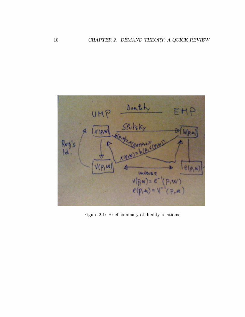
10 CHAPTER 2. DEMAND THEORY: A QUICK REVIEW
Figure 2.1: Brief summary of duality relations

2.1. CONSUMER THEORY 11
x(p;m)! h(p; u) Slutsky:
Dpx(p; u)�Dmx xT = Dph(p; u):
V (p;m)! x(p;m) Roy�s identity:
x(p;m) = � 1
rmV (p;m)rpV (p;m):
e(p; u)! h(p; u) Expenditure function properties:
h(p; u) = rpe(p; u):
V (p;m)$ e(p; u) Utility-expenditure duality, for given p 2 RL++:
V (:;m) = e�1(:;m);
e(:; u) = V �1(:; u)
x(p;m)$ h(p; u) Marshallian-Hicks demand duality:
x(p;m) = h(p; V (p;m))
h(p; u) = x(p; e(p; u))
2.1.2 Aggregate demand
It is useful to study in detail the properties of aggregate demand, as a func-tion of wealth. With some abuse of notation, let introduce the notation toindex agents, i = 1; :::; I. Let the wealth of agent i be denoted mi: Fix thedistribution of wealth as follows,
mi = �im for some given �i � 0, for all i,Xi
�i = 1:
The Marshallian demand of any agent i is then denoted xi(p;mi) and
x(p;m) =Xi2Ixi(p;mi)
is the aggregate demand.
12 CHAPTER 2. DEMAND THEORY: A QUICK REVIEW
Aggregate demand trivially inherits several properties from individualdemand, i.e., di¤erentiability, homeogeneity of degree 0, Walras Law. Butdoes x(p;m) satisfy WARP? Not, typically. Take (p;m) and (p0;m0) suchthat x (p0;m0) 6= x (p;m) and
p � x (p0;m0) � m:
It is immediate to see that the following inequality can still hold:
p0 � x (p;m) � m0
(because p�x (p0;m0) � m does not imply p�xi (p0;mi0) � mi for all i; similarlyfor p0 � x (p;m) � m0.)A su¢ cient condition for aggregate demand x (p;m) to satisfy WARP
is that individual Marshallian demands satisfy the (uncompensated) law ofdemand, that is, substitution e¤ects prevail over income e¤ects.
Proposition 5 Suppose xi(p;mi) satis�es the (uncompensated) law of de-mand, that is,
Dpxi(p;mi) is negative semi-de�nite
for all i: Then x (p;m) also satis�es the (uncompensated) law of demandand hence WARP.
2.2 Producer theory
We shall study the production activity of �rms operating in competitivemarkets. A production plan is a y 2 RL, interpreted as the net output of theL goods:
yi < 0 : input
yi > 0 : output
The production set is the set of (technologically feasible) production plans:
Y � RL:
Whenever the commodities which are outputs in the production set are �xed,O � f1; ::; Lg (and hence also the complementary set of those which are in-puts), the outer boundary of Y can typically be represented by a (continuous)
2.2. PRODUCER THEORY 13
production function, describing the maximal output level attainable for anylevel of inputs. In the case where O = f1g ; e.g.,
y1 = f(z) i¤
(y1;�z) 2 Y@y01 > y1 : (y
01;�z) 2 Y
We assume that Y and and f : RL�1+ ! R+ satisfy the following assump-tions:
Regularity Y is nonempty, closed, Y \ RL+ = f0g (no free lunch andpossibility of inaction), and it satis�es free disposal :
y 2 Y and y0 � y ) y0 2 Y
Correspondingly, f : RL�1+ ! R+ is monotonically increasing.
Convexity Y is strictly convex:
y; y0 2 Y ) �y + (1� �)y0 2 intY
Correspondingly, f : RL�1+ ! R+ is strictly concave (has decreasingreturns to scale). (Y is convex,
y 2 Y ) �y 2 Y for all � 2 [0; 1]
corresponds to f : RL�1+ ! R+ is concave - has non-increasing returnsto scale.)
Any �rm chooses a production plan so as to maximize pro�ts:
max p � ys.t. y 2 Y
Existence of a solution requires conditions ensuring that Y is boundedabove. For every p � 0, a solution induces a net supply correspondencey(p):
Proposition 6 The net supply correspondence y(p) satis�es the followingproperties:

14 CHAPTER 2. DEMAND THEORY: A QUICK REVIEW
y(p) is homogeneous of degree 0 in p;
y(p) is a convex-valued correspondence (a single valued function if f :RL�1+ ! R+ is strictly concave).
The value of the solution is a pro�t function �(p) = p � y(p):
Proposition 7 The pro�t function �(p) satis�es the following properties:
�(p) is homogeneous of degree 1 in p;
�(p) is a convex function.
Proof. The properties are straighforward consequences of the propertiesof y(p): We leave them to the reader, except convexity; which is proved asfollows. Take any pair p0; p00 and consider p̂ = �p0 + (1� �)p00 for � 2 (0; 1).Note that �(p̂) = y(p̂) � (�p0 + (1� �)p00) � �y(p0) � p0 + (1 � �)y(p00) � p00= ��(p0) + (1� �)�(p00):Suppose Y is a convex cone,
y 2 Y ) �y 2 Y for all � > 0;
that is, the technology has constant returns to scale: Correspondingly, theproduction function f : RL�1+ ! R+ is homogeneous of degree 1 in its argu-ments and,
- y 2 y(p)) �y 2 y(p) for all � > 0;
- �(p) = 0 for all p:
Whenever f is di¤erentiable, any solution of the �rm�s problem satisfythe following system of foc�s (stated here for the case of interior solutions):
p1Df = w:
Focs are also su¢ cient if f is concave.Assume f is continuously di¤erentiable and strictly concave. Applying
the Implicit Function theorem to foc�s, we obtain:
Dwz =1
p1
�D2f
��1is symmetric, negative de�nite
Furthermore, by the envelope theorem, y(p) = Dp�, so that Dpy = D2�
is:
2.2. PRODUCER THEORY 15
- symmetric,
- positive - recall z = �(y2; ::; yL) ! - semide�nite (by the convexity of �) and
- such that Dpy p = 0 (by the homogeneity of y(p)).
Let p =�p1w
�and y =
�y1z
�: The input level z which solves the �rm�s
choice problem also solves the following problem:
minz2RL�1+
C = wz
s:t: f(z) � y1:This is perfectly analogous to expenditure minimization problem of con-sumer. Hence we know that:
- C(w; y1) is concave in w and such that @C=@y1 > 0 and @C=@wl � 0;l = 1; ::; L� 1;
- z(w; y1) = DwC exhibits the properties of a compensated demand function.
16 CHAPTER 2. DEMAND THEORY: A QUICK REVIEW
Chapter 3
Arrow-Debreu exchangeeconomies
3.1 The economy
The economy is polupated by I consumers with preferences described byU i : RL+ ! R and resources !i 2 RL+, i 2 I = f1; ::; Ig :1 An allocation is anarray (x1; ::; xI) 2 RLI+ , and it is feasible if it satis�es
IXi=1
xi �IXi=1
!i
In the special case in which L = 2, I = 2, feasible allocations can be graphi-cally represented using the Edgeworth Box.Unless otherwise noted, we shall impose the following strong (but not
outrageous) assumptions.
Assumption 2 U i : RL+ ! R is C2 in any open subset of RL+;strictly monotonicin its arguments and strictly quasi-concave. Furthermore, ! 2 RLI++:
3.2 Pareto e¢ ciency
An allocation x 2 RLI+ is Pareto e¢ cient if it is feasible and there is no otherfeasible allocation x̂ 2 RLI+ which Pareto dominates it:
U i(x̂i) � U i(xi) for all i, > for at least one i.1We are conscious of the notational abuse.
17
18 CHAPTER 3. ARROW-DEBREU EXCHANGE ECONOMIES
Pareto dominance de�nes a (social) preference relation over the set of allo-cations RLI+ , which is however incomplete.PE allocations are solutions of the problem:
maxx Ui(xi)
s.t.P
i xi �
Pi !
i
U i0(xi
0) � �U i
0for all i0 6= i
for some given��U i
0�i0 6=i :
The foc�s (for an interior solution) of this problem are:
rU i = �
�i0rU i0 = � for all i0 6= iXi
xi =Xi
!i
where��i
0�i0 6=i and � are the Lagrange multipliers of the two sets of con-
straints above. Thus
rU i = �i0rU i0 for all i0 6= i
and utility gradients are co-linear for all agents (Marginal rates of substitu-tion are equalized across agents).Varying the values of �U i
0for i0 6= i we obtain the set Pareto e¢ cient
allocations, the Pareto frontier.Let the Utility possibility set be the image of the feasible allocations in
the space of utility levels
U =
(U 2 RI
�����U � �U i(xi)�Ii=1 , for some x 2 RLI+ such thatXi
xi �Xi
!i
)
U is closed, convex, bounded above. Furthermore, the set of Pareto optimalutilities is de�ned as
UP = fU 2 U j@U 0 2 U such that U 0 > U g :2
2In our notation, U 0 > U requires U 0i � U i, for any i 2 I; with at least one strictinequality.
3.3. COMPETITIVE EQUILIBRIUM 19
Theorem 8 (Negishi) Let x 2 RLI+ be a Pareto e¢ cient allocation. Thenthere exist a � 2 RI+, � 6= 0, such that
x = argmaxXi2I�iU i(xi)
s.t.Xi
xi �Xi
!i:
Furthermore,�i
�i0= �i
0; for any i0 6= i 2 I:
Proof. Consider a Pareto optimal allocation x; so that U(x) = fU i(xi)gi2I 2UP. Furthermore, U(x) 2 bdry(U), and U is closed, convex, bounded above.An appropriate separating hyperplane theorem then implies that there existsa � 2 RI , � 6= 0, such that
�U(x) � �U; for any U 2 U;
that is,
U(x) = argmaxXi2I�iU i
s.t. U 2 U:
Trivially, then
x = argmaxXi2I�iU i(xi)
s.t.Xi
xi �Xi
!i:
Finally, U is unbounded below, which implies that � 2 RI+:PE allocations support points on the outer boundary of UP .
3.3 Competitive equilibrium
Agents trade in perfectly competitive markets.

20 CHAPTER 3. ARROW-DEBREU EXCHANGE ECONOMIES
A competitive equilibrium is an allocation x = (:::; xi; ::) 2 RLI+ and aprice p 2 RL++ such that
xi 2 argmaxU i(xi)
s.t. pxi � p!i;
for any i 2 I; and Xi
xi �Xi
!i:
Trade is voluntary, hence equilibrium allocations will satisfy individual ra-tionality:
U i(xi) � U i(!i) for all i = 1; :::; I:Letting mi = p!i we can derive agent I�s Marshallian demand from hisconsumer problem, as in the previous chapter. It is convenient, however,represent demand functions in terms of endowments rather than wealth:
xi : RL++ � RL++ ! RL+:
Let zi (p; !i) denote agent i 2 I�s excess demand: zi (p; !i) = xi (p; !i)� !i:Finally, the aggregate excess demand z : RL++ � RLI++ ! RL+ is de�ned as
z (p; !) =Xi2Izi�p; !i
�:
Proposition 9 For any economy ! 2 RLI++ the aggregate excess demandz (p; !) satis�es the following properties:
smoothness: z (p; !) is C1;
homogeneity of degree 0: z (�p; !) = z (p; !) ;for any � > 0;
Walras Law: pz (p; !) = 0; 8p >> 0;
lower boundedness: 9s such that zl (p; !) > �s, 8l 2 L;
boundary property:
pn ! p 6= 0; with pl = 0 for some l;) max fz1(pn; !); :::; zL(pn; !)g ! 1:
Let�s �rst study the welfare properties of competitive equilibrium alloca-tions.
3.3. COMPETITIVE EQUILIBRIUM 21
Theorem 10 (First welfare) All competitive equilibrium allocations arePareto e¢ cient.
Proof. Suppose x = (::; xi; ::) is a competitive equilibrium allocation forsome price p and it is not Pareto e¢ cient. Then there must be anotherallocation x̂ = (::; x̂i; ::) which is feasible and Pareto dominates x. But sincexi is the optimal choice of consumer i at prices p and preferences are stronglymonotone, U i(x̂i) � U i(xi) implies p�x̂i � p�xi for all i and also, p�x̂i � p�!i,with all the previous inequalities being strict for at least some i. Summingthe latter inequality over i yields p �
Pi x̂
i > p �P
i !i which contradicts the
feasibility of x̂:
Theorem 11 (Second welfare) For any Pareto e¢ cient allocation x 2RLI+ , there exist transfers t 2 RLI , such that
Pi ti = 0 and x 2 RLI+ is a
competitive equilibrium allocation (for some prices p 2 RL++) of the economywith initial endowment ! + t 2 RLI+ .
Proof. Let ti = xi � !i for all i. The theorem is an implication of theseparating hyperplane theorem.Let ! = (!i)i2I denote the vector of aggregate endowments:Competitive
equilibrium prices are solutions of:
z(p;!) �Xi
xi(p; p � !i)�Xi
!i = 0;
a system of L equations in L unknowns, the prices p. By Walras law
p � X
i
xi(p; p � !i)�Xi
!i
!= 0; for all p
and hence at most L � 1 equations are independent (the market clearingequation for one market can be o,itted without loss of generality). By ho-mogeneity of degree 0 in p of xi(p; p � !i); for any i 2 I; prices can always benormalized, e.g., restricted without loss of generality to
p 2 �L�1 �(p 2 RL+ :
Xl
pl = 1
);
the L-simplex, a compact ad convex set.

22 CHAPTER 3. ARROW-DEBREU EXCHANGE ECONOMIES
The equilibrium equations can thus be always reduced to L�1 equationsin L� 1 unknowns. Since equations are typically nonlinear, having numberof unknowns less or equal than number of independent equations does notensure a solution exists.
Theorem 12 (Existence) Let z : �L�1 ! RL be a continuous function,such that p � z(p) = 0 for all p. Then there exists p� such that z(p�) � 0:
Sketch of the proof.
Let 'l(p) =pl +max f0; zl(p)gPL
j=1 [pj +max f0; zj(p)g], l = 1; ::L
Note that �L�1 is convex and compact, and ' : �L�1 ! �L�1. Hence bythe Brouwer Fixed Point theorem there is a �xed point p�:
p�l =p�l +max f0; zl(p�)gPLj=1 [pj +max f0; zj(p)g]
, l = 1; ::L.
Then
zl(p�)p�l
LXj=1
�p�j +max f0; zj(p�)g
�= zl(p
�)p�l + zl(p�)max f0; zl(p�)g
and summing over l yields:
0 =Xl
zl(p�)max f0; zl(p�)g ) zl(p
�) � 0 for all l = 1; :::; L:
Since p� satis�es z(p�) � 0 and Walras law, p� � z(p�) = 0,
zl(p�) < 0 i¤ p�l = 0:
But this is impossible under strong monotonicity and hence:
z(p�) = 0:
To properly claim existence of a competitive equilibrium need to face one lastproblem: the consumers�demand is not de�ned for prices on the boundary of�L�1 (when the price of some good is zero). We need to use a limit argument,considering z : �L�1
" ! RL, for�L�1" �
�p 2 RL+ :
Pl pl = 1, pl � " for all l
,
and taking limits as "! 0.

3.3. COMPETITIVE EQUILIBRIUM 23
3.3.1 Uniqueness
Existence of a competitive equilibrium can be proved under quite general con-ditions.3 Equilibria are however unique only under very strong restrictions.Several examples of such restrictions are listed in the following.
The endowment distribution is Pareto e¢ cient, and hence the only equilib-rium is autarchic: xi = !i for all i 2 I:
Preferences satisfy an aggregation condition (so that a representative con-sumer exists) for all p and for given (mh)Hh=1:
Aggregate demand satis�es WARP and equilibria are locally isolated.
Aggregate demand satis�es the gross substitution property:
p0l > pl and p0j = pj; for all j 6= l;=)
zj(p0) > zj(p).
Note that gross substitution implies that the law of demand holds atany equilibrium price. Gross substitution holds for instance for CobbDouglas and CES utility functions (provided � < 1).
3.3.2 Local uniqueness
Let an economy be parametrized by the endowment vector ! 2 RLI++ keepingpreferences (ui)i2I �xed. Furthermore, normalize pL = 1 and eliminate theL-th component of the excess demand. Then
z : RL�1++ � RLI++ ! RL�1
represents an aggregate excess demand for an exchange economy ! = (!i)i2I 2RLI++.
De�nition 13 A p 2 RL++ such that z (p; !) = 0 is regular if Dpz (p; !)has rank L� 1:
3We shall leave this statement essentially unsubstantiated. General equilibrium theory,for more than half a century, has considered this as one of its main objectives.
24 CHAPTER 3. ARROW-DEBREU EXCHANGE ECONOMIES
De�nition 14 An economy ! 2 RLI++ is regular if Dpz (p; !) has rank L� 1for any p 2 RL�1++ such that z (p; !) = 0.
De�nition 15 An equilibrium price p 2 RL�1++ is locally unique if 9 anopen set P such that p 2 P and for any p0 6= p 2 P , z (p0; !) 6= 0:
Proposition 16 A regular equilibrium price p 2 RL�1++ is locally unique.
Proof. Fix an arbitrary ! 2 RLI++: Since Dpz (p; !) has rank L � 1; byregularity of p, the Inverse function theorem - Local (see Math Appendix)applied to the map z : RL�1++ ! RL�1, directly implies local uniqueness of p 2RL�1++ .
Proposition 17 Any economy ! in a full measure Lebesgue subset of RLI++is regular.
We say then that regularity is a generic property in RLI++, as it holds in afull measure Lebesgue subset of RLI++.Proof. The statement follows by the Transversality theorem (see MathAppendix), if z t 0: We now show that z t 0: Pick an arbitrary agenti 2 I: It will be su¢ cient to show that, for any (p; !) 2 RL�1++ � RLI++ suchthat z(p; !) = 0; we can �nd a perturbation d!i 2 RL such that dz =D!iz(p; !)d!
i, for any dz 2 RL�1. Consider any perturbation d!i such thatd!i1 + pd!
i�1 = 0; for d!i�1 = (!il)
L
l=2 : Any such perturbation, leaves eachagent i 2 I demand unchanged and hence it implies D!iz(p; !)d!
i = �d!i�1,for any arbitrary d!i�1 2 RL:
Proposition 18 The set of equilibrium prices of an economy ! 2 RLI++ is asmooth manifold (see Math Appendix) of dimension LI:
Proof. Dpz (p; !) has rank L � 1, as shown in the proof of the previousproposition. The Inverse function theorem - Global (see Math Appendix)applied to z : RL�1++ � RLI++ ! RL�1; directly implies that the set p 2 z�1(0);as a function of ! 2 RLI++, is a smooth manifold of dimension LI:
3.3. COMPETITIVE EQUILIBRIUM 25
3.3.3 Di¤erentiable approach: A rough primer
The di¤erential techniques exploited to study generic local uniqueness canbe expanded to provide a general characterization of competitive equilibriaas a manifold parametrized by endowments. This characterization implies anexistence result. We sketch some of the analysis, just to provide the readerwith the �avor of the arguments.
De�nition 19 The index i(p; !) of a price p 2 RL�1++ such that z (p; !) = 0is de�ned as
i(p; !) = (�1)L�1sign jDpz (p; !)j :The index i(!) of an economy (!i)i2I is de�ned as
i(!) =X
p:z(p;!)=0
i(p; !):
Theorem 20 (Index) For any regular economy ! 2 RLI++, i(!) = 1:
Proof. The theorem is a deep mathematical result whose proof is clearlybeyond the scope of this class. Let it su¢ ce to say that the proof reliescrucially on the boundary property of excess demand. Adventurous readermight want to look at Mas Colell (1985), section 5,6, p. 201-15.
Corollary 21 Any regular economy ! has an odd number of equilibria. Inparticular, any regular economy ! 2 RLI++ has at least one equilibrium.
Corollary 22 Any economy ! 2 RLI++ has at least one equilibrium price p 2RL�1++ :Proof. By contradiction. Suppose there exist an economy ! 2 RLI++ withno equilibrium. Then, ! 2 RLI++ is regular, by de�nition of regularity - acontradiction with previous corollary.
The existence result is then a corollary of the Index theorem. It is usefulto study the simple case in which L = 2: In this case, then, z : R++ ! R.The boundary properties of the excess demand z(p; !) imply that, for any! 2 R2I++;
z(p; !) ! +1 as p! 0
z(p; !) ! �L as p!1:

26 CHAPTER 3. ARROW-DEBREU EXCHANGE ECONOMIES
As a consequence, an equilibrium exists by continuity of z(p; !). Further-more, suppose ! is regular, and let the prices pj such that z(p; !) = 0 beordered, so that pj < pj+1; j = 1; 2; :::: Then @z(p;!)
@pjp=p1 < 0: Actually,
@z(p;!)@p
���p=pjn < 0 for j odd> 0for j even
: As a consequence, i(!) = 1:
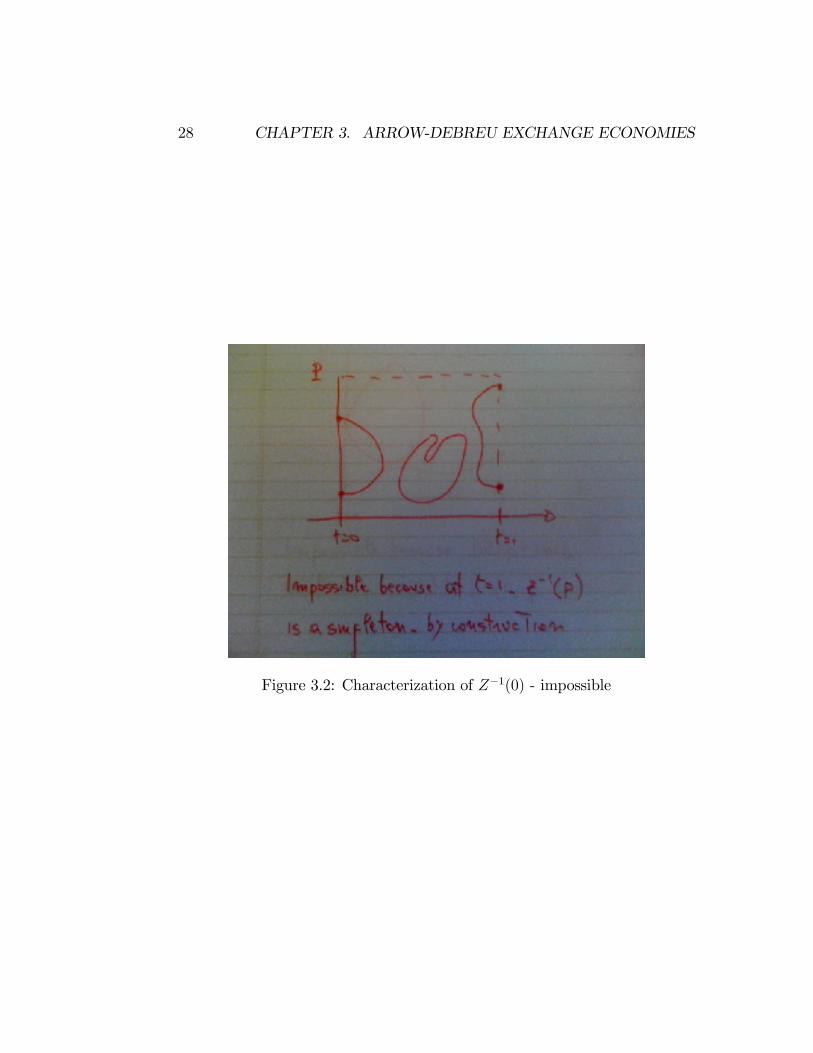
We can also try and give more sense of the arguments, o¤ of the proofof the Index theorem, required for this approach to the existence question.Let ! 2 RLI++ be an arbitrary regular economy. Pick an economy !0 2 RLI++such that there exist a unique price p 2 RL�1++ such that z(p) = 0; andDpz(p) has rank L � 1: One such economy can always be constructed bychoosing !0 2 RLI++ to be a Pareto optimal allocation. In fact, [we can showthat] generic regularity holds in the subset of economies with Pareto optimalendowments. Let t! + (1 � t)!0; for 0 � t � 1; represent a 1-dimensionalsubset of economies. Let Z(p; t) be the map Z : RL�1++ �[0; 1]! RL�1 inducedby Z(p; t) = z(p; t! + (1 � t)!0) for given (!; !0): We say that Z(p; t) is anhomotopy, or that z(p; !) and z(p; !0) are homotopic to each other. [Wecan show that] DZ(p; t) has rank L � 1 in its domain. It follows from theCorollary of the Inverse function theorem - Global (see Math Appendix) thatthe set (p; t) 2 Z�1(0); is a smooth manifold of dimension 1: [We can showthat] prices p can, without loss of generality, be restricted to a compact setP such that Z�1(0)\P � [0; 1] = ?:4 As a consequence Z�1(0) is a compactsmooth manifold of dimension 1: By the Classi�cation theorem (see MathAppendix), Z�1(0) is then homeomorphic to a countable set of segmentsin R and of circles S.5 Regularity of Z�1(0) at the boundary, t = 0 andt = 1 and the property that Z�1(0) \ P � [0; 1] = ? imply that at least onecomponent of Z�1(0) is homeomorphic to a line with boundary at t = 0 andt = 1: It looks confusing, but it�s easier with a few �gures.
The only possible representation of Z�1(0) is then as in the following�gure. Therefore: an equilibrium price p 2 P exists, for any t 2 [0; 1];and furthermore, for a full-measure Lebesgue subset of [0; 1] the number ofequilibria is odd.
4This is a consequence of the boundary conditions of excess demand systems. In otherwords, we could adopt the alternative normalization, restricting prices in the simplex �;a compact set, and show that equilibrium prices are never on @�:
5Along a component of Z�1(0) (a line or a circle), a change in index occurs when themanifold folds.

3.3. COMPETITIVE EQUILIBRIUM 27
Figure 3.1: Characterization of Z�1(0) - impossible
28 CHAPTER 3. ARROW-DEBREU EXCHANGE ECONOMIES
Figure 3.2: Characterization of Z�1(0) - impossible

3.3. COMPETITIVE EQUILIBRIUM 29
Figure 3.3: Characterization of Z�1(0) - impossible

30 CHAPTER 3. ARROW-DEBREU EXCHANGE ECONOMIES
Figure 3.4: Characterization of Z�1(0)
3.4. MATHEMATICAL APPENDIX 31
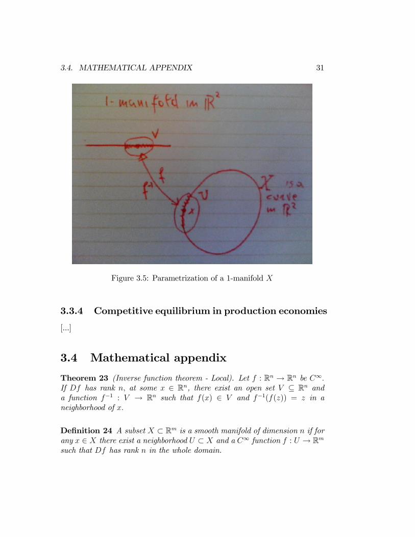
Figure 3.5: Parametrization of a 1-manifold X
3.3.4 Competitive equilibrium in production economies
[...]
3.4 Mathematical appendix
Theorem 23 (Inverse function theorem - Local). Let f : Rn ! Rn be C1:If Df has rank n; at some x 2 Rn, there exist an open set V � Rn anda function f�1 : V ! Rn such that f(x) 2 V and f�1(f(z)) = z in aneighborhood of x:
De�nition 24 A subset X � Rm is a smooth manifold of dimension n if forany x 2 X there exist a neighborhood U � X and a C1 function f : U ! Rmsuch that Df has rank n in the whole domain.

32 CHAPTER 3. ARROW-DEBREU EXCHANGE ECONOMIES
Let f(U) = V: A smooth manifold of dimension n is then locally parame-trized by a restriction of the function f�1 on the open set V \Rn�f0gm�n,in the sense that f�1 maps V \ Rn � f0gm�n onto U; a neighborhood of xon X.
Example 25 An example of a 1-manifold of R2 is S =�x 2 R2
��(x1)2 + (x2)2 = 1,the circle. An explicit parametrization for S can be constructed as follows.Seeing a restriction of f�1on the open set V \ Rn � f0gm�n as a map�i : Rn ! Rm; the following four maps are su¢ cient to parametrize S:
�1(x1) =
�x1;
q1� (x1)2
�if x2 > 0
�2(x1) =
�x1;�
q1� (x1)2
�if x2 < 0
�3(x2) =
�q1� (x2)2; x2
�if x1 > 0
�4(x2) =
��q1� (x2)2; x2
�if x1 < 0
De�nition 26 Let f : Rm ! Rn; m � n; be C1: f is transversal to 0,denoted f t 0; if Df has rank n for any x 2 Rm such that f(x) = 0:
Theorem 27 (Transversality). Let f : Rm++ ! Rn++; m � n; be C1 andtransversal to 0, f t 0: Decompose any vector x 2 Rm++ as x =
�x1x2
�; with
x1 2 Rm�n++ ; x2 2 Rn++: Then Dx2f(x) has rank n for all x in a Lebesguemeasure-1 subset of Rm++:
De�nition 28 A subset X � Rm is a smooth manifold with boundary ofdimension n if for any x 2 X there exist a neighborhood U � X and a C1
function f : U ! Rm�1 �R+ such that Df has rank n in the whole domain.
The boundary @X of X is de�ned by @X = f�1(f0gm�1�R+)\X: It canbe shown that, if X � Rm is a smooth manifold with boundary of dimensionn; then @X is a smooth manifold (without boundary) of dimension n� 1:
Example 29 An example of a smooth manifold with boundary of dimension2 in R2 is S =
�x 2 R2
��(x1)2 + (x2)2 � 1, the sphere. A parametrizationfor can be constructed S, by means of a series of maps �i : R2 ! R2+; alongthe lines of the parametrization of the circle, S: Furthermore, @S =S:

3.4. MATHEMATICAL APPENDIX 33
Figure 3.6: Parametrization of a 2-manifold with boundary

34 CHAPTER 3. ARROW-DEBREU EXCHANGE ECONOMIES
Theorem 30 (Inverse function theorem - Global) Let f : Rm ! Rn;m � n; be C1: Suppose that Dxf has rank n for any x 2 Rm. Then f�1(0) =fx 2 Rm jf(x) = 0g is a smooth manifold of dimension m� n:
Corollary 31 Let f : Rn� [0; 1]! Rn be C1: Suppose that Dxf has rank nfor any (x; t) 2 Rn � [0; 1]. Then f�1(0) = f(x; t) 2 Rn � [0; 1] jf(x; t) = 0gis a smooth 1�manifold with boundary:
Theorem 32 (Classi�cation) Every compact smooth 1�manifold is home-omorphic to a disjoint union of countably many copies of segments in R andof S.
Furthermore, @ f�1(0) = fx 2 Rn jf(x; 0) = 0g [ fx 2 Rn jf(x; 1) = 0g :
3.4.1 References
The main reference is:
A. Mas-Colell (1985): The Theory of General Economic Equilibrium: ADi¤erentiable Approach, Econometric Society Monograph, CambridgeUniversity Press.
But, as Andreu told me once, "I do not hate students so much that Iwould give them this book to read." Similar comments hold, in my opinion,for
Y. Balasko (1988): Foundations of the Theory of General Equilibrium, Aca-demic Press.
You are then left with:
A. Mas-Colell, M. Whinston, and J. Green (1995): Microeconomic Theory,Oxford University Press, ch. 17.D.
A. Mas-Colell, Four Lectures on the Di¤erentiable Approach to GeneralEquilibrium Theory, in A. A. Ambrosetti, F. Gori, and R. Lucchetti(eds.), Lecture Notes in Mathematics, No. 1330, Springer-Verlag, Berlin,1986.
3.5 Strategic foundations
[...]
Chapter 4
Two-period economies
In a two-period pure exchange economy we study �nancial market equilib-ria. In particular, we study the welfare properties of equilibria and theirimplications in terms of asset pricing.In this context, as a foundation for macroeconomics and �nancial eco-
nomics, we study su¢ cient conditions for aggregation, so that the standardanalysis of one-good economies is without loss of generality, su¢ cient condi-tions for the representative agent theorem, so that the standard analysis ofsingle agent economies is without loss of generality.The No-arbitrage theorem and the Arrow theorem on the decentraliza-
tion of equilibria of state and time contingent good economies via �nancialmarkets are introduced as useful means to characterize �nancial market equi-libria.
4.1 Arrow-Debreu economies
Consider an economy extending for 2 periods, t = 0; 1. Let i 2 f1; :::; Igdenote agents and l 2 f1; :::; Lg physical goods of the economy. In addition,the state of the world at time t = 1 is uncertain. Let f1; :::; Sg denote thestate space of the economy at t = 1. For notational convenience we typicallyidentify t = 0 with s = 0, so that the index s runs from 0 to S:De�ne n = L(S+1): The consumption space is denoted then by X � Rn+.
Each agent is endowed with a vector !i = (!i0; !i1; :::; !
iS), where !
is 2 RL+;
for any s = 0; :::S. Let ui : X �! R denote agent i�s utility function. Wewill assume:
35

36 CHAPTER 4. TWO-PERIOD ECONOMIES
Assumption 1 !i 2 Rn++ for all i
Assumption 2 ui is continuous, strongly monotonic, strictly quasiconcaveand smooth, for all i (see Magill-Quinzii, p.50 for de�nitions and details).Furthermore, ui has a Von Neumann-Morgernstern representation:
ui(xi) = ui(xi0) +SXs=1
probsui(xis)
Suppose now that at time 0, agents can buy contingent commodities.That is, contracts for the delivery of goods at time 1 contingently to therealization of uncertainty. Denote by xi = (xi0; x
i1; :::; x
iS) the vector of all
such contingent commodities purchased by agent i at time 0, where xis 2 RL+;for any s = 0; :::; S: Also, let x = (x1; :::; xI):Let � = (�0; �1; :::; �S); where �s 2 RL+ for each s; denote the price of
state contingent commodities; that is, for a price �ls agents trade at time 0the delivery in state s of one unit of good l:Under the assumption that the markets for all contingent commodities
are open at time 0, agent i�s budget constraint can be written as1
�0(xi0 � !i0) +
SXs=0
�s(xis � !is) = 0 (4.1)
De�nition 33 An Arrow-Debreu equilibrium is a (x�; ��) such that
1: x�i 2 argmaxui(xi) s.t. �0(xi0 � !i0) +
SXs=0
�s(xis � !is) = 0; and
2:IXi=1
x�i � !is = 0, for any s = 0; 1; :::; S
Observe that the dynamic and uncertain nature of the economy (con-sumption occurs at di¤erent times t = 0; 1 and states s 2 S) does notmanifests itself in the analysis: a consumption good l at a time t and state sis treated simply as a di¤erent commodity than the same consumption goodl at a di¤erent time t0 or at the same time t but di¤erent state s0. This is
1We write the budget constraint with equality. This is without loss of generality undermonotonicity of preferences, an assumption we shall maintain.
4.1. ARROW-DEBREU ECONOMIES 37
the simple trick introduced in Debreu�s last chapter of the Theory of Value.It has the fundamental implication that the standard theory and results ofstatic equilibrium economies can be applied without change to our dynamic)environment. In particular, then, under the standard set of assumptions onpreferences and endowments, an equilibrium exists and the First and SecondWelfare Theorems hold.2
De�nition 34 Let (x�; ��) be an Arrow-Debreu equilibrium. We say that x�
is a Pareto optimal allocation if there does not exist an allocation y 2 XI
such that
1: u(yi) � u(x�i) for any i = 1; :::; I (strictly for at least one i), and
2:IXi=1
yi � !is = 0, for any s = 0; 1; :::; S
Theorem 35 Any Arrow-Debreu equilibrium allocation x� is Pareto Opti-mal.
Proof. By contradiction. Suppose there exist a y 2 X such that 1) and 2)in the de�nition of Pareto optimal allocation are satis�ed. Then, by 1) inthe de�nition of Arrow-Debreu equilibrium, it must be that
��0(yi0 � !i0) +
SXs=0
��s(yis � !is) � 0;
for all i; and
��0(yi0 � !i0) +
SXs=0
��s(yis � !is) > 0;
for at least one i.Summing over i, then
��0
IXi=1
(yi0 � !i0) +SXs=0
��s
IXi=1
(yis � !is) > 0
which contradicts requirement 2) in the de�nition of Pareto optimal alloca-tion.The proof exploits strict monotonicity of preferences. Where?2Having set de�nitions for 2-periods Arrow-Debreu economies, it should be apparent
how a generalization to any �nite T -periods economies is in fact e¤ectively straightforward.In�nite horizon will be dealt with in successive notes.
38 CHAPTER 4. TWO-PERIOD ECONOMIES
4.2 Financial market economies
Consider the 2-period economy just introduced. Suppose now contingentcommodities are not traded. Instead, agents can trade in spot markets andin j 2 f1; :::; Jg assets. An asset j is a promise to pay ajs � 0 units of goodl = 1 in state s = 1; :::; S.3 Let aj = (a
j1; :::; a
jS): To summarize the payo¤s
of all the available assets, de�ne the S � J asset payo¤ matrix
A =
0@ a11 ::: aJ1::: :::a1S ::: aJS
1A :It will be convenient to de�ne as to be the s-th row of the matrix. Note thatit contains the payo¤ of each of the assets in state s.Let p = (p0; p1; :::; pS), where ps 2 RL+ for each s, denote the spot price
vector for goods. That is, for a price pls agents trade one unit of good lin state s: Recall the de�nition of prices for state contingent commodities inArrow-Debreu economies, denoted �: Note the di¤erence. Let good l = 1at each date and state represent the numeraire; that is, p1s = 1, for alls = 0; :::; S.Let xisl denote the amount of good l that agent i consumes in good s. Let
q = (q1; :::; qJ) 2 RJ+, denote the prices for the assets.4 Note that the pricesof assets are non-negative, as we normalized asset payo¤ to be non-negative.Given prices (p; q) and the asset structure A, any agent i picks a con-
sumption vector xi 2 X and a portfolio zi 2 RJ to
maxui(xi)
s.t.
p0(xi0 � !i0) = �qzi
ps(xis � !is) = Asz
i; for s = 1; :::S:
3The non-negativity restriction on asset payo¤s is just for notational simplicity.4Quantities will be row vectors and prices will be column vectors, to avoid the annoying
use of transposes.

4.2. FINANCIAL MARKET ECONOMIES 39
De�nition 36 A Financial markets equilibrium is a (x�; z�; p�; q�) such that
1: x�i 2 argmaxui(xi) s.t.
p0(xi0 � !i0) = �qzi; and
ps(xis � !is) = asz
i; for s = 1; :::S; and furthermore
2:
IXi=1
x�i � !is = 0, for any s = 0; 1; :::; S; andIXi=1
z�i
Financial markets equilibrium is the equilibrium concept we shall careabout. This is because i) Arrow-Debreu markets are perhaps too demanding arequirement, and especially because ii) we are interested in �nancial marketsand asset prices q in particular. Arrow-Debreu equilibrium will be a usefulconcept insofar as it represents a benchmark (about which we have a wealthof available results) against which to measure Financial markets equilibrium.
Remark 37 The economy just introduced is characterized by asset marketsin zero net supply, that is, no endowments of assets are allowed for. It isstraightforward to extend the analysis to assets in positive net supply, e.g.,stocks. In fact, part of each agent i�s endowment (to be speci�c: the projectionof his/her endowment on the asset span, < A >= f� 2 RS : � = Az; z 2RJg) can be represented as the outcome of an asset endowment, ziw; that is,letting !i1 = (!
i11; :::; !
i1S), we can write
!i1 = wi1 + Az
iw
and proceed straightforwardly by constructing the budget constraints and theequilibrium notion.
No Arbitrage
Before deriving the properties of asset prices in equilibrium, we shall investsome time in understanding the implications that can be derived from themilder condition of no-arbitrage. This is because the characterization of no-arbitrage prices will also be useful to characterize �nancial markets equilbria.For notational convenience, de�ne the (S + 1)� J matrix
W =
��qA
�:
40 CHAPTER 4. TWO-PERIOD ECONOMIES
De�nition 38 W satis�es the No-arbitrage condition if there does not exista
there does not exist a z 2 RJ such that Wz > 0:5
The No-Arbitrage condition can be equivalently formulated in the follow-ing way. De�ne the span of W to be
< W >= f� 2 RS+1 : � = Wz; z 2 RJg:
This set contains all the feasible wealth transfers, given asset structure A.Now, we can say that W satis�es the No-arbitrage condition if
< W >\RS+1+ = f0g:
Clearly, requiring that W = (�q; A) satis�es the No-arbitrage condition isweaker than requiring that q is an equilibrium price of the economy (withasset structure A). By strong monotonicity of preferences, No-arbitrage isequivalent to requiring the agent�s problem to be well de�ned. The nextresult is remarkable since it provides a foundation for asset pricing basedonly on No-arbitrage.
Theorem 39 (No-Arbitrage theorem)
< W >\RS+1+ = f0g () 9�̂ 2 RS+1++ such that �̂W = 0:
First, observe that there is no uniqueness claim on the �̂, just existence.Next, notice how �̂W = 0 implies �̂� = 0 for all � 2< W > : It then providesa pricing formula for assets:
�̂W =
0@ :::
��̂0qj + �̂1aj1 + :::+ �̂SajS
:::
1A =
0@ :::0:::
1AJx1
and, rearranging, we obtain for each asset j,
qj = �1aj1 + :::+ �Sa
jS; for �s =
�̂s�̂0
(4.2)
5Wz > 0 requires that all components of Wz are � 0 and at least one of them > 0:

4.2. FINANCIAL MARKET ECONOMIES 41
Note how the positivity of all components of �̂ was necessary to obtain(4.2).Proof. =) De�ne the simplex in RS+1+ as � = f� 2 RS+1+ :
PSs=0 � s = 1g.
Note that by the No-arbitrage condition, < W >T� is empty. The proof
hinges crucially on the following separating result, a version of Farkas Lemma,which we shall take without proof.
Lemma 40 Let X be a �nite dimensional vector space. Let K be a non-empty, compact and convex subset of X. Let M be a non-empty, closed andconvex subset of X. Furthermore, let K and M be disjoint. Then, thereexists �̂ 2 Xnf0g such that
sup�2M
�̂� < inf�2K
�̂� :
Let X = RS+1+ , K = � and M =< W >. Observe that all the requiredproperties hold and so the Lemma applies. As a result, there exists �̂ 2Xnf0g such that
sup�2<W>
�̂� < inf�2�
�̂� : (4.3)
It remains to show that �̂ 2 RS+1++ : Suppose, on the contrary, that thereis some s for which �̂s � 0. Then note that in (4.3 ), the RHS� 0: By (4.3),then, LHS < 0: But this contradicts the fact that 0 2< W > .We still have to show that �̂W = 0, or in other words, that �̂� = 0 for
all � 2< W >. Suppose, on the contrary that there exists � 2< W > suchthat �̂� 6= 0: Since < W > is a subspace, there exists � 2 R such that�� 2< W > and �̂�� is as large as we want. However, RHS is boundedabove, which implies a contradiction.(= The existence of �̂ 2 RS+1++ such that �̂W = 0 implies that �̂� = 0
for all � 2< W > : By contradiction, suppose 9� � 2< W > and such that� � 2 RS+1+ nf0g: Since �̂ is strictly positive, �̂� � > 0; the desired contradiction.
A few �nal remarks to this section.
Remark 41 An asset which pays one unit of numeraire in state s and noth-ing in all other states (Arrow security), has price �s according to (4.2). Suchasset is called Arrow security.

42 CHAPTER 4. TWO-PERIOD ECONOMIES
Remark 42 Is the vector �̂ obtained by the No-arbitrage theorem unique?Notice how (??) de�nes a system of J equations and S unknowns, representedby �. De�ne the set of solutions to that system as
R(q) = f� 2 RS++ : q = �Ag:
Suppose, the matrix A has rank J 0 � J (that it, A has J 0 linearly independentcolumn vectors and J 0 is the e¤ective dimension of the asset space). Ingeneral, then R(q) will have dimension S � J 0. It follows then that, in thiscase, the No-arbitrage theorem restricts �̂ to lie in a S � J 0 + 1 dimensionalset. If we had S linearly independent assets, the solution set has dimensionzero, and there is a unique � vector that solves (??). The case of S linearlyindependent assets is referred to as Complete markets.
Remark 43 Let preferences be Von Neumann-Morgernstern:
ui(xi) = ui(xi0) +X
s=1;:::;S
probsui(xis)
whereX
s=1;:::;S
probs = 1: Let then ms =�sprobs
. Then
qj = E (mAj)
In this representation of asset prices the vector m 2 RS++ is called Stochasticdiscount factor.
4.2.1 The stochastic discount factor
In the previous section we showed the existence of a vector that provides thebasis for pricing assets in a way that is compatible with equilibrium, albeitmilder than that. In this section, we will strengthen our assumptions andstudy asset prices in a full-�edged economy. Among other things, this willallow us to provide some economic content to the vector �Recall the de�nition of Financial market equilibrium. Let MRSis(x
i)denote agent i�s marginal rate of substitution between consumption of thenumeraire good 1 in state s and consumption of the numeraire good 1 atdate 0:

4.2. FINANCIAL MARKET ECONOMIES 43
MRSis(xi) =
@ui(xis)
@xi1s
@ui(xi0)
@xi10
Let MRSi(xi) = (: : :MRSis(xi) : : :) denote the vector of marginal rates
of substitution for agent i, an S dimentional vector. Note that, under theassumption of strong monotonicity of preferences, MRSi(xi) 2 RS++:By taking the First Order Conditions (necessary and su¢ cient for a max-
imum under the assumption of strict quasi-concavity of preferences) withrespect to zij of the individual problem for an arbitrary price vector q, weobtain that
qj =SXs=1
probsMRSis(x
i)ajs = E�MRSi(xi) � aj
�; (4.4)
for all j = 1; :::; J and all i = 1; :::; I; where of course the allocation xi is theequilibrium allocation. At equilibrium, therefore, the marginal cost of onemore unit of asset j, qj, is equalized to the marginal valuation of that agentfor the asset�s payo¤,
PSs=1 probsMRS
is(x
i)ajs.Compare equation (4.4) to the previous equation (4.2). Clearly, at any
equilibrium, condition (4.4) has to hold for each agent i. Therefore, in equi-librium, the vector of marginal rates of substitution of any arbitrary agent ican be used to price assets; that is any of the agents�vector of marginal ratesof substitution (normalized by probabilities) is a viable stochastic discountfactor m:In other words, any vector (: : : probsMRSis(x
i) : : :) belongs to R(q) and ishence a viable � for the asset pricing equation (4.2). But recall that R(q) is ofdimension S�J 0; where J 0 is the e¤ective dimension of the asset space. Thehigher the the e¤ective dimension of the asset space (sloppily said, the larger�nancial markets) the more aligned are agents�marginal rates of substitutionat equilibrium (sloppily said, the smaller are unexploited gains from tradeat equilibrium). In the extreme case, when markets are complete (that is,when the rank of A is S), the set R(q) is in fact a singleton and hence theMRSi(xi) are equalized across agents i at equilibrium: MRSi(xi) = MRS;for any i = 1; :::; I:
Problem 44 Write the Pareto problem for the economy and show that, atany Pareto optimal allocation, x; it is the case that MRSi(xi) = MRS; for

44 CHAPTER 4. TWO-PERIOD ECONOMIES
any i = 1; :::; I: Furthermore, show that an allocation x which satis�es thefeasibility conditions (market clearing) for goods and is such thatMRSi(xi) =MRS; for any i = 1; :::; I: is Pareto optimal.
We conclude that, when markets are Complete, equilibrium allocationsare Pareto optimal. That is, the First Welfare theorem holds for Financialmarket equilibria when markets are Complete.
Problem 45 (Economies with bid-ask spreads)Extend our basic two-periodincomplete market economy by assuming that, given an exogenous vector 2RJ++:
the buying price of asset j is qj + jwhile
the selling price of asset j is qjfor any j = 1; :::; J:and exogenous. Write the budget constraint and theFirst Order Conditions for an agent i�s problem. Derive an asset pricingequationfor qj in terms of intertemporal marginal rates of substitution atequilibrium.
4.2.2 Arrow theorem
The Arrow theorem is the fondamental decentralization result in �nancialeconomics. It states su¢ cient conditions for a form of equivalence betweenthe Arrow-Debreu and the Financial market equilibrium concepts. It wasessentially introduced by Arrow (1952). The proof of the theorem introducesa reformulation of the budget constraints of the Financial market economywhich focuses on feasible wealth transfers across states directly, on the spanof A,
< A >=�� 2 RS : � = Az; z 2 RJ
in particular. Such a reformulation is important not only in itself but as alemma for welfare analysis in Financial market economies.
Proposition 46 Let (x�; ��) represent an Arrow-Debreu equilibrium. Sup-pose rank(A) = S (�nancial markets are Complete). Then (x�; z�; p�; q�) isa Financial market equilibrium, where
��s = �sp�s; for any s = 1; :::; S: and
q� =
SXs=1
probsMRSis(x
i�)As
4.2. FINANCIAL MARKET ECONOMIES 45
Futhermore, the converse also holds: if (x�; z�; p�; q�) is a Financial marketequilibrium of an economy with rank(A) = S, (x�; ��) represents an Arrow-Debreu equilibrium, where ��s = �sp
�s; for any s = 1; :::; S:
Proof. Financial market equilibrium prices of assets q� satisfy No-arbitrage.There exists then a vector �̂ 2 RS+1++ such that �̂W = 0; or q� = �A. Thebudget constraints in the �nancial market economy are
p�0�xi�0 � !i0
�+ q�zi� = 0
p�s�xi�s � !is
�= Asz
i�; for s = 1; :::S:
Substituting q = �A; expanding the �rst equation, and writing the con-straints at time 1 in vector form, we obtain:
p�0�xi�0 � !i0
�+
SXs=1
�sp�s
�xi�s � !is
�= 0 (4.5)266664
::
p�s (xi�s � !is)::
377775 2 < A > (4.6)
But if rank(A) = S; it follows that< A >= RS; and the constraint
266664::
p�s (xi�s � !is)::
377775 2<A > is never binding. Each agent i�s problem is then subject only to
p�0�xi�0 � !i0
�+
SXs=1
�sp�s
�xi�s � !is
�= 0;
the budget constraint in the Arrow-Debreu economy with
��s = �sp�s; for any s = 1; :::; S:
Furthermore, by No-arbitrage
q� =
SXs=1
probsMRSis(x
i�)As:

46 CHAPTER 4. TWO-PERIOD ECONOMIES
Finally, using �s = probsMRSis(x
i�), for any s = 1; :::; S; proves the re-sult. (Recall that, with Complete markets MRSi(xi�) = MRS; for anyi = 1; :::; I.)The converse is straightforward.
4.2.3 Existence
We do not discuss here in detail the issue of existence of a �nancial marketequilibrium when markets are incomplete (when they are complete, existencefollows from the equivalence with Arrow-Debreu equilibrium provided byArrow theorem). A sketch of the proof however follows.The proof is a modi�cation of the existence proof for Arrow-Debreu equi-
librium. By Arrow theorem, fact, we can reduce the equilibrium system to anexcess demand system for consumption goods; that is, we can solve out for theasset portfolios zi�s. The only conceptual problem with the proof is that theboundary condition on the excess demand system might not be guaranteed as
each agent�s excess demand is restricted by
266664::
ps (xis � !is)::
377775 2< A > : Thisis where the Cass trick comes in handy. It is in fact an important Lemma.
Cass trick. For any Financial market economy, consider a modi�ed econ-
omy where the constraint
266664::
ps (xis � !is)::
377775 2< A > is imposed on all
agents i = 2; :::; I but not on agent i = 1: Any equilibrium of theFinancial Market economy is an equilibrium of the modi�ed economy,and any equilibrium of the modi�ed economy is a Financial marketequilibrium.
Proof. Consider an equilibrium of the modi�ed economy in the state-ment. At equilibrium,
PIi=1 ps (x
is � !is) = 0: Therefore,
PIi=2 ps (x
is � !is) =

4.2. FINANCIAL MARKET ECONOMIES 47
�ps (x1s � !1s) : But
266664::
ps (xis � !is)::
377775 2< A >; for any i = 2; :::; I; and
hencePI
i=2 ps (xis � !is) 2< A > : Since
PIi=2 ps (x
is � !is) = �ps (x1s � !1s) ;
it follows that �ps (x1s � !1s) 2< A >; and hence that ps (x1s � !1s) 2<A > : Therefore, the constraint ps (x1s � !1s) 2< A > must necessarily holdat an equilibrium of the modi�ed economy. In other words, the constraintps (x
1s � !1s) 2< A > is not binding at a Financial market equilibrium. The
equivalence between the modi�ed economy and the Financial Market econ-omy is now straightforward.
4.2.4 Constrained Pareto optimality
Under Complete markets, the First Welfare Theorem holds for Financialmarket equilibrium. This is a direct implication of Arrow theorem.
Proposition 47 Let (x�; z�; p�; q�) be a Financial market equilibrium of aneconomy with Complete markets (with rank(A) = S): Then x� is a Paretooptimal allocation.
However, under Incomplete markets Financial market equilibria are gener-ically ine¢ cient in a Pareto sense. That is, a planner could �nd an allocationthat improves some agents without making any other agent worse o¤.
Theorem 48 At a Financial Market Equilibrium (x�; z�; p�; q�) of an incom-plete �nancial market economy, that is, of an economy with rank(A) < S,the allocation x� is generically6 not Pareto Optimal.
6We say that a statement holds generically when it holds for a full Lebesgue-measuresubset of the parameter set which characterizes the economy. In these notes we shallassume that the an economy is parametrized by the endowments for each agent, the assetpayo¤ matrix, and a two-parameter parametrization of utility functions for each agent;see Magill-Shafer, ch. 30 in W. Hildenbrand and H. Sonnenschein (eds.), Handbook ofMathematical Economics, Vol. IV, Elsevier, 1991.
48 CHAPTER 4. TWO-PERIOD ECONOMIES
Proof. From the proof of Arrow theorem, we can write the budget con-straints of the Financial market equilibrium as:
p�0�xi�0 � !i0
�+
SXs=1
�sp�s
�xi�s � !is
�= 0 (4.7)266664
::
p�s (xi�s � !is)::
377775 2 < A > (4.8)
for some � 2 RS++: Pareto optimality of x�requires that there does not existan allocation y such that
1: u(yi) � u(x�i) for any i = 1; :::; I (strictly for at least one i), and
2:IXi=1
yi � !is = 0, for any s = 0; 1; :::; S
Reproducing the proof of the First Welfare theorem, it is clear that, if such
a y exists, it must be that
266664::
p�s (yi�s � !is)::
377775 =2< A >; for some i = 1; :::; I;otherwise the allocation y would be budget feasible for all agent i at theequilibrium prices. Generic Pareto sub-optimality of x� follows then directlyfrom the following Lemma, which we leave without proof.7
Lemma 49 Let (x�; z�; p�; q�) represent a Financial Market Equilibrium ofan economy with rank(A) < S: For a generic set of economies, the con-
straints
266664::
p�s (xi�s � !is)::
377775 2< A > are binding for some i = 1; :::; I.7The proof can be found in Magill-Shafer, ch. 30 in W. Hildenbrand and H. Sonnen-
schein (eds.), Handbook of Mathematical Economics, Vol. IV, Elsevier, 1991. It requiresmathematical tecniques from di¤erential topology which are not appropriate to be intro-duced in this course.

4.2. FINANCIAL MARKET ECONOMIES 49
Remark 50 The Lemma implies a slightly stronger result than generic Paretosub-optimality of Financial market equilibrium for economies with incompletemarkets. It implies in fact that a Pareto improving allocation can be foundlocally around the equilibrium, as a perturbation of the equilibrium.
Pareto optimality might however represent too strict a de�nition of socialwelfare of an economy with frictions which restrict the consumption set, as inthe case of incomplete markets. In this case, markets are assumed incompleteexogenously. There is no reason in the fundamentals of the model why theyshould be, but they are. Under Pareto optimality, however, the social welfarenotion does not face the same contraints. For this reason, we typically de�ne aweaker notion of social welfare, Constrained Pareto optimality, by restrictingthe set of feasible allocations to satisfy the same set of constraints on theconsumption set imposed on agents at equilibrium. In the case of incompletemarkets, for instance, the feasible wealth vectors across states are restrictedto lie in the span of the payo¤ matrix. That can be interpreted as theeconomy�s ��nancial technology�and it seems reasonable to impose the sametechnological restrictions on the planner�s reallocations. The formalizationof an e¢ ciency notion capturing this idea follows. Let xit=1 = (x
is)Ss=1 2 RSL+ ;
and similarly pt=1 = (ps)Ss=1 2 RSL+
De�nition 51 (Diamond, 1968; Geanakoplos-Polemarchakis, 1986) Let (x�; z�; p�; q�)represent a Financial market equilibrium of an economy whose consumptionset at time t = 1 is restricted by
xit=1;2 B(pt=1); for any i = 1; :::; I
In this economy, the allocation x� is Constrained Pareto optimal if there doesnot exist a (y; �) such that
1: u(yi) � u(x�i) for any i = 1; :::; I, strictly for at least one i
2:IXi=1
yis � !is = 0, for any s = 0; 1; :::; S
and3: yit=1 2 B(g�t=1(!; �)); for any i = 1; :::; I
where g�t=1(!; �) is a vector of equilibrium prices for spot markets at t = 1opened after each agent i = 1; :::; I has received income transfer A�i:

50 CHAPTER 4. TWO-PERIOD ECONOMIES
The constraint on the consumption set restricts only time 1 consump-tion allocations. More general constraints are possible but these formulationis consistent with the typical frictions we encounter in economics, e.g., on�nancial markets. It is important that the constraint on the consumptionset depends in general on g�t=1(!; �), that is on equilibrium prices for spotmarkets opened at t = 1 after income transfers to agents. It implicit identi-�es income transfers (besides consumption allocations at time t = 0) as theinstrument available for Constrained Pareto optimality; that is, it implicitlyconstrains the planner implementing Constraint Pareto optimal allocationsto interact with markets, speci�cally to open spot markets after transfers.On the other hand, the planner is able to anticipate the spot price equilib-rium map, g�t=1(!; �); that is, to internalize the e¤ects of di¤erent transferson spot prices at equilibrium.
Proposition 52 Let (x�; z�; p�; q�) represent a Financial market equilibriumof an economy with complete markets (rank(A) = S) and whose consumptionset at time t = 1 is restricted by
xit=1 2 B � RSL+ ; for any i = 1; :::; I
In this economy, the allocation x� is Constrained Pareto optimal.
Crucially, markets are complete and B is independent of prices. Theproof is then a straightforward extension of the First Welfare theorem com-bined with Arrow theorem.8 Constraint Pareto optimality of Financial mar-ket equilibrium allocations is guaranteed as long as the constraint set B isexogenous.
Proposition 53 Let (x�; z�; p�; q�) represent a Financial market equilibriumof an economy with Incomplete markets (rank(A) < S). In this economy,the allocation x� is not Constrained Pareto optimal.
Proof. By the decomposition of the budget constraints in the proof of Arrowtheorem, this economy is equivalent to one with Complete markets whoseconsumption set at time t = 1 is restricted by
xit=1 2 B(g�t=1(!; z)); for any i = 1; :::; I; for any i = 1; :::; I8To be careful, we need to guarantee that monotonicity of preferences on RSL++ results
in monotonicity on B � RSL++: This is the case for B open. Thanks to the students fornoticing this.
4.2. FINANCIAL MARKET ECONOMIES 51
with the set B(g�t=1(!; z)) de�ned implicitly by266664::
g�s(!s; z) (xis � !is)
::
377775 2< A >; for any i = 1; :::; INote �rst of all that, by construction, p�s 2 g�s(!s; z�): Following the proof ofPareto sub-otimality of Financial market equilibrium allocations, it then fol-
lows that if a Pareto-improving y exists, it must be that
266664::
p�s (yi�s � !is)::
377775 =2<
A >; for some i = 1; :::; I; while
266664::
g�s(!s; �) (yis � !is)
::
377775 = A�i, for all
i = 1; :::; I: Generic Constrained Pareto sub-optimality of x� follows thendirectly from the following Lemma, which we leave without proof.9
Lemma 54 Let (x�; z�; p�; q�) represent a Financial Market Equilibrium ofan economy with rank(A) < S: For a generic set of economies, the con-
straints
266664::
g�s(!s; z� + dz) (yis � !is)
::
377775 = A (zi� + dzi), for some dz 2 RJIn f0gsuch that
Xi=1I
dzi = 0; are weakly relaxed for all i = 1; :::; I, strictly for at
least one.10
9The proof is due to Geanakoplos-Polemarchakis (1986). It also requires di¤erentialtopology techniques.10Once again, note that the Lemma implies that a Pareto improving allocation can be
found locally around the equilibrium, as a perturbation of the equilibrium.

52 CHAPTER 4. TWO-PERIOD ECONOMIES
There is a fundamental di¤erence between incomplete market economies,which have typically not Constrained Optimal equilibrium allocations, andeconomies with constraints on the consumption set, which have, on the con-trary, Constrained Optimal equilibrium allocations. It stands out by com-paring the respective trading constraints
g�s(!s; �)(xis�!is) = As�i; for all i and s, vs. xit=1 2 B, for all i:
The trading constraint of the incomplete market economy is determined atequilibrium, while the constraint on the consumption set is exogenous. An-other way to re-phrase the same point is the following. A planner choosing(y; �) will take into account that at each (y; �) is typically associated a dif-ferent trading constraint g�s(!s; �)(x
is � !is) = As�i; for all i and s; while any
agent i will choose (xi; zi) to satisfy p�s(xis � !is) = Aszi; for all s, taking as
given the equilibrium prices p�s:The constrained ine¢ ciency due the dependence of constraints on equilib-
rium prices is sometimes called a pecuniary externality.11 Several examples ofsuch form of externality/ine¢ ciency have been developed recently in macro-economics. Some examples are:
- Thomas, Charles (1995): "The role of �scal policy in an incomplete marketsframework," Review of Economic Studies, 62, 449�468.
- Krishnamurthy, Arvind (2003): "Collateral Constraints and the Ampli�-cation Mechanism,"
Journal of Economic Theory, 111(2), 277-292.
- Caballero, Ricardo J. and Arvind Krishnamurthy (2003): "Excessive Dol-lar Debt: Financial Development and Underinsurance," Journal of Fi-nance, 58(2), 867-94.
- Lorenzoni, Guido (2008): "Ine¢ cient Credit Booms," Review of EconomicStudies, 75 (3), 809-833.
- Kocherlakota, Narayana (2009): "Bursting Bubbles: Consequences andCauses,"
http://www.econ.umn.edu/~nkocher/km_bubble.pdf.
11The name is due to Joe Stiglitz (or is it Greenwald-Stiglitz?).

4.2. FINANCIAL MARKET ECONOMIES 53
- Davila, Julio, Jay Hong, Per Krusell, and Victor Rios Rull (2005): "Con-strained E¢ ciency in the Neoclassical Growth Model with UninsurableIdiosyncractic Shocks," mimeo, University of Pennsylvania.
Remark 55 Consider an economy whose constraints on the consumption setdepend on the equilibrium allocation:
xit=1 2 B(x�t=1; z�); for any i = 1; :::; I
This is essentially an externality in the consumption set. It is not hard toextend the analysis of this section to show that this formulation introducesine¢ ciencies and equilibrium allocations are Constraint Pareto sub-optimal.
Corollary 56 Let (x�; z�; p�; q�) represent a Financial market equilibrium ofa 1-good economy (L = 1) with Incomplete markets (rank(A) < S). In thiseconomy, the allocation x� is Constrained Pareto optimal.Proof. The constraint on the consumption set implied by incomplete mar-kets, if L = 1, can be written
(xis � !is) = Aszi:
It is independent of prices, of the form xit=1 2 B.
Remark 57 Consider an alternative de�nition of Constrained Pareto opti-mality, due to Grossman (1970), in which constraints 3 are substituted by
30:
266664::
p�s (xi�s � !is)::
377775 = Azi; for any i = 1; :::; Iwhere p� is the spot market Financial market equilibrium vector of prices.That is, the planner takes the equilibrium prices as given. It is immediate toprove that, with this de�nition of Constrained Pareto optimality, any Finan-cial market equilibrium allocation x�of an economy with Incomplete marketsis in fact Constrained Pareto optimal, independently of the �nancial marketsavailable (rank(A) � S):

54 CHAPTER 4. TWO-PERIOD ECONOMIES
Problem 58 Consider a Complete market economy (rank(A) = S) whosefeasible set of asset portfolios is restricted by:
zi 2 Z ( RJ ; for any i = 1; :::; I
A typical example is borrowing limits:
zi � �b; for any i = 1; :::; I
Are equilibrium allocations of such an economy Constrained Pareto optimal(also if L > 1)?
Problem 59 Consider a 1-good (L = 1) Incomplete market economy (rank(A) <S) which lasts 3 periods. De�ne an Financial market equilibrium for thiseconomy as well as Constrained Pareto optimality. Are Financial marketequilibrium allocations of such an economy Constrained Pareto optimal?
Problem 60 Extend our basic two-period incomplete market economy by as-suming that, given an exogenous vector 2 RJ++:
the buying price of asset j is qj + j
whilethe selling price of asset j is qj
for any j = 1; :::; J:and exogenous. 1) Suppose the asset payo¤ matrix isfull rank. Do you expect �nancial market equilibria to be Pareto e¢ cient?Carefully justify your answer. (I am not asking for a formal proof, thoughyou could actually prove this.) 2) Continue to suppose the asset payo¤ matrixis full rank. How would you de�ne Constrained Pareto e¢ ciency in thiseconomy? Do you expect �nancial market equilibria to be Constrained Paretoe¢ cient? Carefully justify your answer. (I am really not asking for a formalproof.)
4.2.5 Aggregation
Agent i�s optimization problem in the de�nition of Financial market equi-librium requires two types of simultaneous decisions. On the one hand, theagent has to deal with the usual consumption decisions i.e., she has to decidehow many units of each good to consume in each state. But she also has

4.2. FINANCIAL MARKET ECONOMIES 55
to make �nancial decisions aimed at transferring wealth from one state tothe other. In general, both individual decisions are interrelated: the con-sumption and portfolio allocations of all agents i and the equilibrium pricesfor goods and assets are all determined simultaneously from the system ofequations formed by (??) and (??). The �nancial and the real sectors ofthe economy cannot be isolated. Under some special conditions, however,the consumption and portfolio decisions of agents can be separated. Thisis typically very useful when the analysis is centered on �nancial issue. Inorder to concentrate on asset pricing issues, most �nance models deal in factwith 1-good economies, implicitly assuming that the individual �nancial de-cisions and the market clearing conditions in the assets markets determinethe �nancial equilibrium, independently of the individual consumption deci-sions and market clearing in the goods markets; that is independently of thereal equilibrium prices and allocations. In this section we shall identify theconditions under which this can be done without loss of generality. This issometimes called "the problem of aggregation."The idea is the following. If we want equilibrium prices on the spot
markets to be independent of equilibrium on the �nancial markets, thenthe aggregate spot market demand for the L goods in each state s shouldmust depend only on the incomes of the agents in this state (and not inother states) and should be independent of the distribution of income amongagents in this state.
Theorem 61 Budget Separation. Suppose that each agent i�s prefer-ences are separable across states, identical, homothetic within states, andvon Neumann-Morgenstern; i.e. suppose that there exists an homotheticu : RL ! R such that
ui(xi) = u(xi0) +SXs=1
probsu(xis); for all i = 1; ::; I:
Then equilibrium spot prices p� are independent of asset prices q and of theincome distribution; that is, constant in
n!i 2 RL(S+1)++
���PIi=1 !
i giveno:
Proof. Normalize all spot prices of good 1: p10 = p1s = 1; for any s 2 S:The consumer�s maximization problem in the de�nition of Financial marketequilibrium can be decomposed into a sequence of spot commodity alloca-tion problems and an income allocation problem as follows. The spot com-modity allocation problems. Given the current and anticipated spot prices
56 CHAPTER 4. TWO-PERIOD ECONOMIES
p = (p0; p1; :::; pS) and an exogenously given stream of �nancial incomeyi = (yi0; y
i1; :::; y
iS) 2 RS+1++ in units of numeraire, agent i has to pick a
consumption vector xi 2 RL(S+1)+ to
maxui(xi)s.t.p0x
i0 = y
i0
psxis = y
is; for s = 1; :::S:
Let the L(S + 1) demand functions be given by xils(p; yi), for l = 1; :::; L;
s = 0; 1; :::S. De�ne now the indirect utility function for income by
vi(yi; p) = ui(xi(p; yi)):
The Income allocation problem. Given prices (p; q); endowments !i, and theasset structure A, agent i has to pick a portfolio zi 2 RJ and an incomestream yi 2 RS+1++ to
max vi(yi; p)s:t:p0!
i0 � qzi = yi0
ps!is + asz
i = yis; for s = 1; :::S:
By additive separability across states of the utility, we can break the con-sumption allocation problem into S+1 �spot market�problems, each of whichyields the demands xis(ps; y
is) for each state. By homotheticity, for each
s = 0; 1; :::S; and by identical preferences across all agents,
xis(ps; yis) = y
isxis(ps; 1);
and since preferences are identical across agents,
yisxis(ps; 1) = y
isxs(ps; 1)
Adding over all agents and using the market clearing condition in spot mar-kets s, we obtain, at spot markets equilibrium,
xs(p�s; 1)
IXi=1
yis �IXi=1
!is = 0:
4.2. FINANCIAL MARKET ECONOMIES 57
Again by homothetic utility,
xs(p�s;
IXi=1
yis)�IXi=1
!is = 0: (4.9)
Recall from the consumption allocation problem that psxis = yis; for s =0; 1; :::S: By adding over all agents, and using market clearing in the spotmarkets in state s,
IXi=1
yis = p�s
IXi=1
xis; for s = 0; 1; :::S (4.10)
= p�s
IXi=1
!is; for s = 0; 1; :::S:
By combining (4.9) and (4.10), we obtain
xs(p�s; p
�s
IXi=1
!is) =IXi=1
!is: (4.11)
Note how we have passed from the aggregate demand of all agents in theeconomy to the demand of an agent owning the aggregate endowments. Ob-serve also how equation (4.11) is a system of L equations with L unknownsthat determines spot prices p�s for each state s independently of asset pricesq: Note also that equilibrium spot prices p�s de�ned by (4.11) only depend !
i
throughPI
i=1 !is:
The Budget separation theorem can be interpreted as identifying condi-tions under which studying a single good economy is without loss of gener-ality. To this end, consider the income allocation problem of agent i, givenequilibrium spot prices p�:
maxyi2RS+1++ ;zi2RJ
vi(yi; p�)
s.t. yi0 = p�0!i0 � qzi
yis = p�s!is + asz
i; for s = 1; :::S
If preferences ui(xi) are identical, homothetic within states, and von Neumann-Morgenstern, that is, if they satisfy
ui(xi) = u(xi0) +
SXs=1
probsu(xis); with u(x) homothetic, for all i = 1; ::; I
58 CHAPTER 4. TWO-PERIOD ECONOMIES
it is straightforward to show that indirect preferences vi(yi; p�) are alsoidentical, homothetic within states, and von Neumann-Morgenstern:
vi(yi; p�) = v(yi0; p�)+
SXs=1
probsv(yis; p
�); with v(y; p�) homothetic, for all i = 1; ::; I:
Let wi0 = p�0!
i0; w
is = p
�s!
is; for any s = 1; :::; S; and disregard for notational
simplicity the dependence of v(y; p�) on p�: The income allocation problemcan be written as:
maxyi2RS+1++ ;zi2RJ
v(yi0) +SXs=1
probsv(yis)
s.t. yi0 � wi0 = �qzi
yis � wis = Aszi; for s = 1; :::S
which is homeomorphic to any agent i�s optimization problem in the de�-nition of Financial market equilibrium with l = 1. Note that yis gains theinterpretation of agent i�s consumption expenditure in state s, while wis isinterpreted as agent i�s income endowment in state s:
The representative agent theorem
A representative agent is the following theoretical construct.
De�nition 62 Consider a Financial market equilibrium (x�; z�; p�; q�) of aneconomy populated by i = 1; :::; I agents with preferences ui : X ! R andendowments !i: A Representative agent for this economy is an agent withpreferences UR : X ! R and endowment !R such that the Financial marketequilibrium of an associated economy with the Representative agent as theonly agent has prices (p�; q�).
In this section we shall identify assumptions which guarantee that theRepresentative agent construct can be invoked without loss of generality.This assumptions are behind much of the empirical macro/�nance literature.
Theorem 63 Representative agent. Suppose preferences satisfy:
ui(xi) = u(xi0) +SXs=1
probsu(xis); with homothetic u(x); for all i = 1; ::; I:

4.2. FINANCIAL MARKET ECONOMIES 59
Let p� denote equilibrium spot prices. If
266664::
p�s!is
::
377775 2< A >; then there exista map uR : RS+1+ ! R such that:
!R =IXi=1
!is;
UR(x) = uR(y0) +SXs=1
probsuR(ys); where ys = p�
IXi=1
xis; s = 0; 1; :::; S
constitutes a Representative agent.
Since the Representative agent is the only agent in the economy, herconsumption allocation and portfolio at equilibrium,
�x�R; z�R
�; are:
x�R = !R =IXi=1
!i
z�R = 0
If the Representative agent�s preferences can be constructed indepen-dently of the equilibrium of the original economy with I agents, then equilib-rium prices can be read out of the Representative agent�s marginal rates ofsubstitution evaluated at
PIi=1 !
i. SincePI
i=1 !i is exogenously given, equi-
librium prices are obtained without computing the consumption allocationand portfolio for all agents at equilibrium, (x�; z�):Proof. The proof is constructive. Under the assumptions on preferences inthe statement, we need to show that, for all agents i = 1; :::; I, equilibrium as-set prices q� are constant in
n!i 2 RL(S+1)++
���PIi=1 !
i giveno.If preferences sat-
isfy ui(xi) = u(xi0) +PS
s=1 probsu(xis); for all i = 1; ::; I, with an homothetic
u(x); then by the Budget separation theorem, equilibrium spot prices p� are
independent of q� and constant inn!i 2 RL(S+1)++
���PIi=1 !
i giveno: There-
fore,
266664::
p�s!is
::
377775 2< A > can be written as an assumption on fundamentals;

60 CHAPTER 4. TWO-PERIOD ECONOMIES
in particular on !i: Furthermore, we can restrict our analysis to the singlegood economy, whose agent i�s optimization problem is:
maxyi2RS+1++ ;zi2RJ
v(yi0) +SXs=1
probsv(yis)
s.t. yi0 � w0 = �qzi
yis � ws = Aszi; for s = 1; :::S
where v(y) is homothetic.We show next that uR(y) = v(y) and !R =
PIi=1 !
is constitute a Repre-
sentative agent. By Arrow theorem�we can write budget constraints as
yi0 � wi0 +SXs=1
�s�yis � wis
�= 0266664
::
yis � wis::
377775 2 < A >
But,
266664::wis::
377775 2< A > implies that there exist a ziw such that266664::wis::
377775 = Aziw:
Therefore,
266664::wis::
377775 2< A > implies that yis = As (zi + ziw), for any s 2 S:Wecan then write each agent i�s optimization problem in terms of (yi0; z
i); andthe value of agent i0s endowment is wi0 +
PSs=1 �sw
is = w
i0 +
PSs=1 �sasz
iw =
wi0 + qziw:
In summary, we write the budget constraint as:
yi0 +
SXs=1
�syis = w
i0 + �sAsz
iw = w
i0 + qz
iw:
4.2. FINANCIAL MARKET ECONOMIES 61
By the fact that preferences are identical across agents and by homo-theticity of v(y); then we can write
yi0�q; wi0
�=
�wi0 + qz
iw
�y0 (q; 1)
yis�q; wi0
�=
�wi0 + qz
iw
�ys (q; 1) ; for any s 2 S
At equilibrium then
y0 (q; 1)Xi2I
�wi0 + qz
iw
�= y0
q;Xi2I
�wi0 + qz
iw
�!=Xi2Iwi0
ys (q; 1)Xi2I
�wi0 + qz
iw
�= ys
q;Xi2I
�wi0 + qz
iw
�!= As
Xi2Iziw; for any s 2 S
and prices q� only depend onPI
i=1wi0 and
PIi=1 z
iw:
Make sure you understand where we used the assumption
266664::
p�!is::
377775 =266664::wis::
377775 2< A > . Convince yourself that the assumption is necessary in theproof.The Representative agent theorem, as noted, allows us to obtain equilib-
rium prices without computing the consumption allocation and portfolio forall agents at equilibrium, (x�; z�):Let w =
PIi=1w
i: Under the assumptionsof the Representative agent theorem, let w0 =
Pi2I w
i0; and ws =
Pi2I w
is;
for any s 2 S: Then
q =SXs=1
probsMRSs(w)As; for MRSs(w) =@v(ws)@ws@v(w0)@w0
That is, asset prices can be computed from agents� preferences uR = v :R! R and from the aggregate endowment (w0; :::; ws; :::) : This is called theLucas�trick for pricing assets.

62 CHAPTER 4. TWO-PERIOD ECONOMIES
Problem 64 Note that, under the Complete markets assumption, the span
restriction on endowments,
266664::
p�!is::
377775 2< A >; for all agents i; is trivially
satis�ed. Does this assumption imply Pareto optimal allocations in equilib-rium?
Problem 65 Assume all agents have identical quadratic preferences. Derive
individual demands for assets (without assuming
266664::
p�!is::
377775 2< A >) and
show that the Representative agent theorem is obtained.
Another interesting but misleading result is the "weak" representativeagent theorem, due to Constantinides (1982).
Theorem 66 Suppose markets are complete (rank(A) = S) and preferencesui(xi) are von Neumann-Morgernstern (but not necessarily identical nor ho-mothetic). Let (x�; z�; p�; q�) be a Financial markets equilibrium. Then,
!R =IXi=1
!i;
UR(x) = max(xi)Ii=1
IXi=1
�iui(xi) s.t.IXi=1
xi = x;
where �i = (�i)�1 and �i =
@ui(xi�)
@xi�10
constitutes a Representative agent.
Clearly, then,
q =SXs=1
probsMRSs(w)As; for MRSs(w) =@UR(ws)@ws
@UR(w0)@w0
:
4.2. FINANCIAL MARKET ECONOMIES 63
Proof. Consider a Financial market equilibrium (x�; z�; p�; q�). By completemarkets, the First welfare theorem holds and x� is a Pareto optimal alloca-tion. Therefore, there exist some weights that make x� the solution to theplanner�s problem. It turns out that the required weights are given by
�i =
�@ui(xi�)
@xi�10
��1:
This is left to the reader to check; it�s part of the celebrated Negishi theorem.
This result is certainly very general, as it does not impose identical ho-mothetic preferences, however, it is not as useful as the �real�Representativeagent theorem to �nd equilibrium asset prices. The reason is that to de�nethe speci�c weights for the planner�s objective function, (�i)Ii=1; we need toknow what the equilibrium allocation, x�; which in turn depends on the wholedistribution of endowments over the agents in the economy.
4.2.6 Asset pricing
Relying on the aggregation theorem in the previous section, in this sectionwe will abstract from the consumption allocation problems and concentrateon one-good economies. This allows us to simplify the equilibrium de�nitionas follows.
4.2.7 Some classic representation of asset pricing
Often in �nance, especially in empirical �nance, we study asset pricing rep-resentation which express asset returns in terms of risk factors. Factors areto be interpreted as those component of the risks that agents do require ahigher return to hold.How do we go from our basic asset pricing equation
q = E(mA)
to factors?
Single factor beta representation
Consider the basic asset pricing equation for asset j;
qj = E(maj)

64 CHAPTER 4. TWO-PERIOD ECONOMIES
Let the return on asset j, Rj, be de�ned as Rj =Ajqj. Then the asset pricing
equation becomes1 = E(mRj)
This equation applied to the risk free rate, Rf , becomes Rf = 1Em. Using the
fact that for two random variables x and y, E(xy) = ExEy + cov(x; y), wecan rewrite the asset pricing equation as:
ERj =1
Em� cov(m;Rj)
Em= Rf � cov(m;Rj)
Em
or, expressed in terms of excess return:
ERj �Rf = �cov(m;Rj)
Em
Finally, letting
�j = �cov(m;Rj)
var(m)
and
�� =var(m)
Em
we have the beta representation of asset prices:
ERj = Rf + �j�m (4.12)
We interpret �j as the "quantity" of risk in asset j and �m (which is thesame for all assets j) as the "price" of risk. Then the expected return ofan asset j is equal to the risk free rate plus the correction for risk, �j�m.Furthermore, we can read (4.12) as a single factor representation for assetprices, where the factor is m, that is, if the representative agent theoremholds, her intertemporal marginal rate of substitution.
Multi-factor beta representations
A multi-factor beta representation for asset returns has the following form:
ERj = Rf +FXf=1
�jf�mf(4.13)

4.2. FINANCIAL MARKET ECONOMIES 65
where (mf )Ff=1 are orthogonal random variables which take the interpretation
of risk factors and
�jf = �cov(mf ; Rj)
var(mf )
is the beta of factor f , the loading of the return on the factor f .
Proposition 67 A single factor beta representation
ERj = Rf + �j�m
is equivalent to a multi-factor beta representation
ERj = Rf +
FXf=1
�jf�mfwith m =
FXf=1
bfmf
In other words, a multi-factor beta representation for asset returns isconsistent with our basic asset pricing equation when associated to a linearstatistical model for the stochastic discount factor m, in the form of m =PF
f=1 bfmf .
Proof. Write 1 = E(mRj) as Rj = Rf � cov(m;Rj)
Emand then to substitute
m =PF
f=1 bfmf and the de�nitions of �jf , to have
�mf=var(mf )bfEmf
The CAPM
The CAPM is nothing else than a single factor beta representation of thefollowing form:
ERj = Rf + �jf�mf
wheremf = a+ bR
w
the return on the market portfolio, the aggregate portfolio held by the in-vestors in the economy.
66 CHAPTER 4. TWO-PERIOD ECONOMIES
It can be easily derived from an equilibrium model under special assump-tions.For example, assume preferences are quadratic:
u(xio; xi1) = �
1
2(xi � x#)2 � 1
2�
SXs=1
probs(xis � x#)2
Moreover, assume agents have no endowments at time t = 1. LetPI
i=1 xis =
xs; s = 0; 1; :::; S; andPI
i=1wi0 = w0. Then budget constraints include
xs = Rws (w0 � x0)
Then,
ms = �xs � x#x0 � x#
=�(w0 � x0)(x0 � x#)
Rws ��x#
x0 � x#
which is the CAPM for a = � �x#
x0�x# and b =�(w0�x0)(x0�x#) :
Note however that a = �x#
x0�x# and b =�(w0�x0)(x0�x#) are not constant, as they
do depend on equilibrium allocations. This will be important when we studyconditional asset market representations, as it implies that the CAPM isintrinsically a conditional model of asset prices.
Bounds on stochastic discount factors
Write the beta representation of asset returns as:
ERj �Rf = cov(m;Rj)
Em=�(m;Rj)�(m)�(Rj)
Em
where 0 � �(m;Rj) � 1 denotes the correlation coe¢ cient and �(:), thestandard deviation. Then
j ERj �Rf�(Rj)
j� �(m)
Em
The left-hand-side is the Sharpe-ratio of asset j.The relationship implies a lower bound on the standard deviation of any
stochastic discount factor m which prices asset j. Hansen-Jagannathan areresponsible for having derived bounds like these and shown that, when thestochastic discount factor is assumed to be the intertemporal marginal rate

4.2. FINANCIAL MARKET ECONOMIES 67
of substitution of the representative agent (with CES preferences), the datadoes not display enough variation in m to satisfy the relationship.
A related bound is derived by noticing that no-arbitrage implies the ex-istence of a unique stochastic discount factor in the space of asset payo¤s,denoted mp, with the property that any other stochastic discount factor msatis�es:
m = mp + �
where � is orthogonal to mp.The following corollary of the No-arbitrage theorem leads us to this result.
Corollary 68 Let (A; q) satisfy No-arbitrage. Then, there exists a unique� � 2< A > such that q = A� �:
Proof. By the No-arbitrage theorem, there exists � 2 RS++ such that q = �A:We need to distinguish notationally a matrix M from its transpose, MT :Wewrite then the asset prices equation as qT = AT�T . Consider �p:
�Tp = A(ATA)�1q:
Clearly, qT = AT�Tp ; that is, �Tp satis�es the asset pricing equation. Further-
more, such �Tp belongs to < A >, since �Tp = Azp for zp = (ATA)�1q: Prove
uniqueness.We can now exploit this uniqueness result to yield a characterization of
the �multiplicity�of stochastic discount factors when markets are incomplete,and consequently a bound on �(m). In particular, we show that, for a given(q; A) pair a vector m is a stochastic discount factor if and only if it canbe decomposed as a projection on < A > and a vector-speci�c componentorthogonal to < A >. Moreover, the previous corollary states that such aprojection is unique.
Let m 2 RS++ be any stochastic discount factor, that is, for any s =1; : : : ; S, ms =
�sprobs
and qj = E(mAj); for j = 1; :::; J: Consider the orthogo-nal projection of m onto < A >, and denote it by mp. We can then write anystochastic discount factors m as m = mp + ", where " is orthogonal to anyvector in < A >; in particular to any Aj. Observe in fact that mp+ " is alsoa stochastic discount factors since qj = E((mp+")aj) = E(mpaj)+E("aj) =E(mpaj), by de�nition of ". Now, observe that qj = E(mpaj) and that wejust proved the uniqueness of the stochastic discount factors lying in < A > :

68 CHAPTER 4. TWO-PERIOD ECONOMIES
In words, even though there is a multiplicity of stochastic discount factors,they all share the same projection on < A >. Moreover, if we make the eco-nomic interpretation that the components of the stochastic discount factorsvector are marginal rates of substitution of agents in the economy, we caninterpret mp to be the economy�s aggregate risk and each agents " to be theindividual�s unhedgeable risk.It is clear then that
�(m) � �(mp)
the bound on �(m) we set out to �nd.
4.2.8 Production
Assume for simplicity that L = 1, and that there is a single type of �rm in theeconomy which produces the good at date 1 using as only input the amountk of the commodity invested in capital at time 0:12 The output depends onk according to the function f(k; s), de�ned for k 2 K, where s is the staterealized at t = 1. We assume that
- f(k; s) is continuously di¤erentiable, increasing and concave in k;
- �; K are closed, compact subsets of R+ and 0 2 K.
In addition to �rms, there are I types of consumers. The demand side ofthe economy is as in the previous section, except that each agent i 2 I is alsoendowed with �i0 units of stock of the representative �rm. Consumer i hasvon Neumann-Morgernstern preferences over consumption in the two dates,represented by ui (xi0) + Eui (xi), where ui (�) is continuously di¤erentiable,strictly increasing and strictly concave.
Competitive equilibrium
Let the outstanding amount of equity be normalized to 1: the initial distri-bution of equity among consumers satis�es
Pi �i0 = 1. The problem of the
�rm consists in the choice of its production plan k:.
12It should be clear from the analysis which follows that our results hold unalteredif the �rms� technology were described, more generally, by a production possibility setY � RS+1.

4.2. FINANCIAL MARKET ECONOMIES 69
Firms are perfectly competitive and hence take prices as given. The�rm�s cash �ow, f(k; s); varies with k. Thus equity is a di¤erent �product�for di¤erent choices of the �rm. What should be its price when all thiscontinuum of di¤erent �products�are not actually traded in the market? Inthis case the price is only a �conjecture.�It can be described by a map Q(k)specifying the market valuation of the �rm�s cash �ow for any possible valueof its choice k.13 The �rm chooses its production plan k so as to maximizeits value. The �rm�s problem is then:
maxk�k +Q(k) (4.14)
When �nancial markets are complete, the present discounted valuation ofany future payo¤ is uniquely determined by the price of the existing assets.This is no longer true when markets are incomplete, in which case the pricesof the existing assets do not allow to determine unambiguously the value ofany future cash �ow. The speci�cation of the price conjecture is thus moreproblematic in such case. Let k� denote the solution to this problem.At t = 0, each consumer i chooses his portfolio of �nancial assets and of
equity, zi and �i respectively, so as to maximize his utility, taking as giventhe price of assets, q and the price of equity Q. In the present environment aconsumer�s long position in equity identi�es a �rm�s equity holder, who mayhave a voice in the �rm�s decisions. It should then be treated as conceptuallydi¤erent from a short position in equity, which is not simply a negativeholding of equity. To begin with, we rule out altogether the possibility ofshort sales and assume that agents can not short-sell the �rm equity:
�i � 0; 8i (4.15)
The problem of agent i is then:
maxxi0;x
i;zi;�iui�xi0�+ Eui
�xi�
(4.16)
subject to (4.15) and
xi0 = !i0 + [�k +Q] �i0 �Q�i � q zi (4.17)
xi(s) = !i(s) + f(k; s)�i + A(s)zi; 8s 2 S (4.18)
13These price maps are also called price perceptions.

70 CHAPTER 4. TWO-PERIOD ECONOMIES
Let�xi�0 ; x
i�; zi�; �i��denote the solution to this problem.
In equilibrium, the following market clearing conditions must hold, forthe consumption good:14X
i
xi0 + k �Xi
!i0Xi
xi(s) �Xi
!i(s) + f(k; s); 8s 2 S
or, equivalently, for the assets: Xi
zi = 0 (4.19)Xi
�i = 1 (4.20)
In addition, the equity price map faced by �rms must satisfy the followingconsistency condition:
i) Q(k�) = Q;
This condition requires that, at equilibrium, the price of equity conjec-tured by �rms coincides with the price of equity, faced by consumers in themarket: �rms�conjectures are �correct�in equilibrium.We also restrict out of equilibrium conjectures by �rms, requiring that
they satisfy:
ii) Q(k) = maxi E [MRSi�f(k)], 8k, whereMRSi� denotes the marginal rateof substitution between consumption at date 0 and at date 1 in states for consumer i; evaluated at his equilibrium consumption allocation(xi�0 ; x
i�).
Condition ii) says that for any k (not just at equilibrium!) the value ofthe equity price map Q(k) equals the highest marginal valuation - across allconsumers in the economy - of the cash �ow associated to k. The consumers�
14We state here the conditions for the case of symmetric equilibria, where all �rms takethe same production and �nancing decision, so that only one type of equity is availablefor trade to consumers. They can however be easily extended to the case of asymmetricequilibria as, for instance, in the example of Section ??.
4.2. FINANCIAL MARKET ECONOMIES 71
marginal rates of substitutions MRSi(s) used to determine the market val-
uation of the future cash �ow of a �rm are taken as given, una¤ected bythe �rm�s choice of k. This is the sense in which, in our economy, �rms arecompetitive: each �rm is �small�relative to the mass of consumers and eachconsumers holds a negligible amount of shares of the �rm.To better understand the meaning of condition ii), note that the con-
sumers with the highest marginal valuation for the �rm�s cash �ow whenthe �rm chooses k are those willing to pay the most for the �rm�s equity inthat case and the only ones willing to buy equity - at the margin - whenits price satis�es ii). Given i) such property is clearly satis�ed for the �rms�equilibrium choice k�. Condition ii) requires that the same is true for anyother possible choice k: the value attributed to equity equals the maximumany consumer is willing to pay for it. Note that this would be the equilibriumprice of equity of a �rm who were to �deviate�from the equilibrium choiceand choose k instead: the supply of equity with cash �ow corresponding tok is negligible and, at such price, so is its demand.In this sense, we can say that condition ii) imposes a consistency con-
dition on the out of equilibrium values of the equity price map; that is, itcorresponds to a "re�nement" of the equilibrium map, somewhat analogousto bacward induction. Equivalently, when price conjectures satisfy this con-dition, the model is equivalent to one where markets for all the possible typesof equity (that is, equity of �rms with all possible values of k) are open, avail-able for trade to consumers and, in equilibrium all such markets - except theone corresponding to k� - clear at zero trade.15
It readily follows from the consumers��rst order conditions that in equi-librium the price of equity and of the �nancial assets satisfy:
Q = maxiE�MRSi� � f(k�)
�(4.21)
q = E�MRSi� � A
�The de�nition of competitive equilibrium is stated for simplicity for the
case of symmetric equilibria, where all �rms choose the same production plan.When the equity price map satis�es the consistency conditions i) and ii) the�rms�choice problem is not convex. Asymmetric equilibria might therefore
15An analogous speci�cation of the price conjecture has been earlier considered byMakowski (1980) and Makowski-Ostroy (1987) in a competitive equilibrium model withdi¤erentiated products, and by Allen-Gale (1991) and Pesendorfer (1995) in models of�nancial innovation.

72 CHAPTER 4. TWO-PERIOD ECONOMIES
exist, in which di¤erent �rms choose di¤erent production plans. The proofof existence of equilibria indeed requires that we allow for such asymmetricequilibria, so as to exploit the presence of a continuum of �rms of the sametype to convexify �rms�choice problem. A standard argument allows thento show that �rms�aggregate supply is convex valued and hence that theexistence of (possibly asymmetric) competitive equilibria holds.
Proposition 69 A competitive equilibrium always exist.
Objective function of the �rm
Starting with the initial contributions of Diamond (1967), Dreze (1974),Grossman-Hart (1979), and Du¢ e-Shafer (1986), a large literature has dealtwith the question of what is the appropriate objective function of the �rmwhen markets are incomplete.The issue arises because, as mentioned above,�rms�production decisions may a¤ect the set of insurance possibilities avail-able to consumers by trading in the asset markets.If agents are allowed in�nite short sales of the equity of �rms, as in the
standard incomplete market model, a small �rm will possibly have a largee¤ect on the economy by choosing a production plan with cash �ows which,when traded as equity, change the asset span. It is clear that the pricetaking assumption appears hard to justify in this context, since changes inthe �rm�s production plan have non-negligible e¤ects on allocations and henceequilibrium prices. The incomplete market literature has struggled with thisissue, trying to maintain a competitive equilibrium notion in an economicenvironment in which �rms are potentially large.In the environment considered in these notes, this problem is avoided
by assuming that consumers face a constraint preventing short sales, (4.15),which guarantees that each �rm�s production plan has instead a negligible(in�nitesimal) e¤ect on the set of admissible trades and allocations availableto consumers. Evidently, for price taking behavior to be justi�ed a no shortsale constraint is more restrictive than necessary and a bound on short salesof equity would su¢ ce; see Bisin-Gottardi-Ruta (2009).When short sales are not allowed, the decisions of a �rm have a negligible
e¤ect on equilibrium allocations and market prices. However, each �rm�s de-cision has a non-negligible impact on its present and future cash �ows. Pricetaking can not therefore mean that the price of its equity is taken as givenby a �rm, independently of its decisions. However, as argued in the previous
4.2. FINANCIAL MARKET ECONOMIES 73
section, the level of the equity price associated to out-of-equilibrium valuesof k is not observed in the market. It is rather conjectured by the �rm. In acompetitive environment we require such conjecture to be consistent, as re-quired by condition ii) in the previous section. This notion of consistency ofconjectures implicitly requires that they be competitive, that is, determinedby a given pricing kernel, independent of the �rm�s decisions.16 But whichpricing kernel? Here lies the core of the problem with the de�nition of the ob-jective function of the �rm when markets are incomplete. When markets areincomplete, in fact, the marginal valuation of out-of-equilibrium productionplans di¤ers across di¤erent agents at equilibrium. In other words, equityholders are not unanimous with respect to their preferred production planfor the �rm. The problem with the de�nition of the objective function of the�rm when markets are incomplete is therefore the problem of aggregatingequity holders�marginal valuations for out-of-equilibrium production plans.The di¤erent equilibrium notions we �nd in the literature di¤er primarily inthe speci�cation of a consistency condition on Q (k), the price map whichthe �rms adopts to aggregate across agents�marginal valuations.17
Consider for example the consistency condition proposed by Dreze (1974):
QD(k) = E
"Xi
�i�MRSi�f(k)
#; 8k (4.22)
Such condition requires the price conjecture for any plan k to equal thepro rata marginal valuation of the agents who at equilibrium are the �rm�sequity holders (that is, the agents who value the most the plan chosen by�rms in equilibrium). It does not however require that the �rm�s equityholders are those who value the most any possible plan of the �rm, withoutcontemplating the possibility of selling the �rm in the market, to allow thenew equity buyers to operate the production plan they prefer. Equivalently,the value of equity for out of equilibrium production plans is determined usingthe - possibly incorrect - conjecture that the �rms�equilibrium shareholderswill still own the �rm out of equilibrium.
16Independence of the kernel is guarantee by the fact that MRSi�(s); for any i, isevaluated at equilibrium.17A minimal consistency condition on Q (k) is clearly given by i) in the previous section,
which only requires the conjecture to be correct in correspondence to the �rm�s equilibriumchoice. Du¢ e-Shafer (1986) indeed only impose such condition and �nd a rather largeindeterminacy of the set of competitive equilibria.

74 CHAPTER 4. TWO-PERIOD ECONOMIES
Grossman-Hart (1979) propose another consistency condition and hencea di¤erent equilibrium notion. In their case
QGH(k) = E
"Xi
�i0MRSi�f(k)
#; 8k
We can interpret such notion as describing a situation where the �rm�s planis chosen by the initial equity holders (i.e., those with some predeterminedstock holdings at time 0) so as to maximize their welfare, again withoutcontemplating the possibility of selling the equity to other consumers whovalue it more. Equivalently, the value of equity for out of equilibrium pro-duction plans is again derived using the conjecture belief that �rms�initialshareholders stay in control of the �rm out of equilibrium.
Unanimity
Under the de�nition of equilibrium proposed in these notes, equity holdersunanimously support the �rm�s choice of the production and �nancial deci-sions which maximize its value (or pro�ts), as in (4.14). This follows fromthe fact that, when the equity price map satis�es the consistency conditionsi) and ii), the model is equivalent to one where a continuum of types of equityis available for trade to consumers, corresponding to any possible choice ofk the representative �rm can make, at the price Q(k). Thus, for any pos-sible value of k a market is open where equity with a payo¤ f(k; s) can betraded, and in equilibrium such market clears with a zero level of trades forthe values of k not chosen by the �rms.For any possible choice k of a �rm, the (marginal) valuation of the �rm
by an agent i isE�MRSi� � f(k�)
�;
and it is always weakly to the market value of the �rm, given by
maxiE�MRSi� � f(k�)
�:
Proposition 70 At a competitive equilibrium, equity holders unanimouslysupport the production k�; that is, every agent i holding a positive initialamount �i0 of equity of the representative �rm will be made - weakly - worseo¤ by any other choice k0 of the �rm.

4.2. FINANCIAL MARKET ECONOMIES 75
E¢ ciency
A consumption allocation (xi0; xi)Ii=1 is admissible if:
18
1. it is feasible: there exists a production plan k such thatXi
xi0 + k �Xi
!i0 (4.23)Xi
xi(s) �Xi
!i(s) + f(k; s); 8s 2 S (4.24)
2. it is attainable with the existing asset structure: for each consumer i,there exists a pair
�zi; �i
�such that:
xi(s) = !i(s) + f(k; s) �i + A(s)zi; 8s 2 S (4.25)
Next we present the notion of e¢ ciency restricted by the admissibilityconstraints:
Constrained e¢ ciency. A competitive equilibrium allocation is constrainedPareto e¢ cient if we can not �nd another admissible allocation whichis Pareto improving.
The validity of the First Welfare Theorem with respect to such notioncan then be established by an argument essentially analogous to the one usedto establish the Pareto e¢ ciency of competitive equilibria in Arrow-Debreueconomies.
First welfare theorem. Competitive equilibria are constrained Pareto ef-�cient.
18To keep the notation simple, we state both the de�nition of competitive equilibria andadmissible allocations for the case of symmetric allocations. The analysis, including thee¢ ciency result ,extends however to the case where asymmetric allocations are allowed areadmissible; see also the next section.
76 CHAPTER 4. TWO-PERIOD ECONOMIES
Modigliani-Miller
We examine now the case where �rms take both production and �nancialdecisions, and equity and debt are the only assets they can �nance theirproduction with. The choice of a �rm�s capital structure is given by thedecision concerning the amount B of bonds issued. The problem of the �rmconsists in the choice of its production plan k and its �nancial structure B.To begin with, we assume without loss of generality that all �rms�debt is riskfree. The �rm�s cash �ow in this context is then [f(k; s)�B] and varies withthe �rm�s production and �nancing choices, k;B. Equity price conjectureshave the form Q(k;B), while the price of the (risk free) bond is independentof (k;B); we denote it p. The �rm�s problem is then:
maxk;B
�k +Q(k;B) + p B (4.26)
The consumption side of the economy is the same as in the previoussection, except that now agents can also trade the bond. Let bi denote thebond portfolio of agent i; and let continue to impose no-short sales contraints:
�i � 0
bi � 0; 8i:
Proceeding as in the previous section, at equilibrium we shall require that
Q(k) = maxiE�MRSi� � [f(k)�B]
�;8k;
p = maxiE�MRSi�
�whereMRSi� denotes the marginal rate of substitution between consumptionat date 0 and at date 1 in state s for consumer i; evaluated at his equilibriumconsumption allocation (xi�0 ; x
i�). Suppose now that �nancial markets arecomplete, that is rank(A) = S: At equilibrium then MRSi� = MRS�, 8i.Therefore, in this case
Q(k;B) + p B = E [MRS� � f(k)] ;8k;
and the value of the �rm, Q(k;B) + p B; is independent of B: This provesthe celebrated
Modigliani-Miller theorem. If �nancial markets are complete the �nanc-ing decision of the �rm, B; is indeterminate.
4.2. FINANCIAL MARKET ECONOMIES 77
It should be clear that when �nancial markets are not complete and agentsare restricted by no-short sales constraints, the Modigliani-Miller theoremdoes not quite necessarily hold.

78 CHAPTER 4. TWO-PERIOD ECONOMIES
Chapter 5
Asymmetric information
Do competitive insurance markets function orderly in the presence of moralhazard and adverse selection? What are the properties of allocations at-tainable as competitive equilibria of such economies? And in particular, arecompetitive equilibria incentive e¢ cient?For such economies the interaction between the private information di-
mension (e.g., the unobservable action in the moral hazard case, the unob-servable type in the adverse selection case) and the observability of agents�trades plays a crucial role, since trades have typically informational con-tent over the agents�private information. In particular, to decentralize in-centive e¢ cient Pareto optimal allocations the availability of fully exclusivecontracts, i.e., of contracts whose terms (price and payo¤) depend on thetransactions in all other markets of the agent trading the contract, is gener-ally required. The implementation of these contracts imposes typically thevery strong informational requirement that all trades of an agent need to beobserved.The fundamental contribution on competitive markets for insurance con-
tracts is Prescott and Townsend (1984). They analyze Walrasian equilibriaof economies with moral hazard and with adverse selection when exclusivecontracts are enforceable, that is, when trades are fully observable.1�In these
1The standard strategic analysis of competition in insurance economies, due toRothschild-Stiglitz (1976), considers the Nash equilibria of a game in which insurancecompanies simultaneously choose the contracts they issue, and the competitive aspect ofthe market is captured by allowing the free entry of insurance companies. Such equi-librium concept does not perform too well: equilibria in pure strategies do not exist forrobust examples (Rothschild-Stiglitz (1976)), while equilibria in mixed strategies exist
79

80 CHAPTER 5. ASYMMETRIC INFORMATION
notes we concentrate on the simpler case of moral hazard. We refer to Bisin-Gottardi (2006) for the case of adverse selection.
5.1 A simple insurance economy
Agents live two periods, t = 0; 1; and consume a single consumption goodonly in period 1. Uncertainty is purely idiosyncratic and all agents are ex-ante identical. In particular, each agent faces a (date 1) endowment whichis an identically and independently distributed random variable ! on a �nitesupport S.2
Moral hazard (hidden action) is captured by the assumption that theprobability distribution of the period 1 endowment that each agent facesdepends from the value taken by a variable e 2 E, an unobservable level ofe¤ort which is chosen by the agent.Let probs(e) be the probability of the realization !s given e. ObviouslyPs2S probs(e) = 1; for any e 2 E; a compact, convex set: By the Law of
Large Numbers, probs(e) is also the fraction of agents who have chosen e¤orte for which state s is realized. Agents�preferences are represented by a vonNeumann-Morgenstern utility function of the following form:X
s2Sprobs(e)u(xs) � v(e)
where v(e) denotes the disutility of e¤ort e. We assume the followingregularity conditions:The utility function u(x) is strictly increasing, strictly concave, twice
continuously di¤erentiable, and limx!0 u0(x) = 1: The cost function v(e)
is strictly increasing, strictly convex, twice continuously di¤erentiable, andsupe2E v
0(e) =1:
(Dasgupta-Maskin (1986)) but, in this set-up, are of di¢ cult interpretation. Even whenequilibria in pure strategies do exist, it is not clear that the way the game is modelled isappropriate for such markets, since it does not allow for dynamic reactions to new contracto¤ers (Wilson (1977) and Riley (1979); see also Maskin-Tirole (1992)). Moreover, oncesequences of moves are allowed, equilibria are not robust to �minor�perturbations of theextensive form of the game (Hellwig (1987)).
2Measurability issues arise in probability spaces with a continuum of indipendent ran-dom variables. We adopt the usual abuse of the Law of Large Numbers.

5.1. A SIMPLE INSURANCE ECONOMY 81
Essentially without loss of generality, let the state space S be ordered sothat !s > !s�1; for all s = 2; :::; S: We then impose the following standardrestriction.
Single-crossing property. The odds ratio probss(e)probss�1(e)
is strictly increasingin e, for any s = 2; :::; S:
5.1.1 The Symmetric information benchmark
Consider now the benchmark case of symmetric information, in which e iscommonly observed. An allocation (x; e) 2 RS+�E of consumption and e¤ortis optimal under symmetric information if it solves:
maxx;e
Xs2S
probs(e)u(xs) � v(e); (5.1)
s.t. Xs2S
probs(e)(xs � !s) = 0
Let qs(e) denote the (linear) price of consumption in state s for agentswho chose e¤ort e. By allowing the prices of the securities whose payo¤ iscontingent on the idiosyncratic uncertainty to depend on e, we e¤ectivelyare introducing price conjectures: we read qs(e) as the price of consumptioncontingent to state s if the agent chooses e¤ort e, for any e 2 E; not justat the equilibrium e. This is the same problem we found in productioneconomies with incomplete markets, where the price faced by the �rm was awhole map Q(k); interpreted as a price conjecture.At a competitive equilibrium each agent solves
maxx;e
Xs2S
probs(e)u(xs) � v(e); (5.2)
s.t. Xs2S
qs(e)(xs � !s) = 0
and markets clear Xs2S
probs(e)(xs � !s) = 0 (5.3)
We impose the following consistency condition on the price conjecture:

82 CHAPTER 5. ASYMMETRIC INFORMATION
qs(e) = probs(e):
Under the consistency condition it is now straightforward to prove theFirst and Second Welfare theorems for this economy under symmetric infor-mation.
5.2 The moral hazard economy
Consider now the case of asymmetric information, in which his choice ofe¤ort e is private information of each agent. In this context, an allocation(x; e) 2 RS+�E of consumption and e¤ort is incentive constrained optimal ifit solves:
maxx;e
Xs2S
probs(e)u(xs) � v(e); (5.4)
s.t. Xs2S
probs(e)(xs � !s) = 0
and
e 2 e(x) = argmaxXs2S
probs(e)u(xs) � v(e); given x
The last constraint, called incentive constraint, requires that the allocation(x; e) must be such that the agent prefers (x; e) to any other allocation (x; e0),for any e; e0 2 E.At a Prescott-Townsend competitive equilibrium prices cannot have the
form qs(e), as the agent�s choice for e is not observed. What is observed,however is the consumption allocation x demanded by the agent in the mar-ket. (Note that the exclusivity assumption guarantees that this is the case,that x is observable). Price conjectures can then be de�ned as a function ofx as
qs(x) = qs(e(x)):
At a competitive equilibrium then each agent solves
maxx;e
Xs2S
probs(e)u(xs) � v(e); (5.5)

5.2. THE MORAL HAZARD ECONOMY 83
s.t.Xs2S
qs(x)(xs � !s) = 0
where qs(x) = qs(e (x)) and e(x) = argmaxXs2S
probs(e)u(xs) � v(e)
and markets clear Xs2S
probs(e)(xs � !s) = 0 (5.6)
At an equilibrium we also impose the following consistency condition onthe price conjecture:
qs(e(x)) = probs(e(x))
The First and Second Welfare theorems, in its incentive constrained versions,hold straightforwardly for the moral hazard economy.An equivalent notion of equilibrium is possible, which is equivalent to
the one just proposed. It is a (sort of) mechanism design formulation of thecompetitive equilibrium. Since prices cannot depend on e¤ort e, which is un-observable, they depend on agents�message/declaration about e¤ort, whichwe denote m 2 E and which his optimally chosen by the agents themselves.An agent declaring m will face prices qs(m) but also a restriction on thespace of allocations B(m) � RS++ designed to guarantee that his declarationcoincides with his e¤ort choice, that is, designed to guarantee truth-telling:m = e:Speci�cally, we write the agent�s problem as follows:
maxx2RS++;(e;m)2E2
Xs2S
probs(e)u(xs) � v(e); (5.7)
s.t.Xs2S
qs(m)(xs � !s) = 0 and x 2 B(m);
where B(m) =
(x 2 RS++ : m 2 argmax
"2E
Xs2S
probs(")u(xs) � v("))
At equilibrium then markets clearXs2S
probs(e)(xs � !s) = 0: (5.8)
84 CHAPTER 5. ASYMMETRIC INFORMATION
In other words, the truth-telling constraint, x 2 B(m), requires that in themarket with prices q(m) only incentive compatible allocations are o¤ered,that is, only allocations which induce the agent to choose e¤ort m; for anym 2 E:3 It is straightforward to see that this equilibrium notion is equivalentto the one with rational price conjectures we have proposed. The interpre-tation is di¤erent however: with rational conjectures it is the conjectureson prices of non incentive compatible allocations which are restricted, whilewith the equilibrium notion in this remark it is tradable allocations whichare restricted to exclude non incentive compatible ones.It is important to note that the allocation (xs)s2S is assumed observable.
This corresponds to the exclusivity case, as it is called in the literature. Thenext problem deals with the non-exclusivity case in a simple but instructiveexample.
Problem 71 In the context of these moral hazard economies M. Harris andR. Townsend (1981) prove a version of the Revelation principle. Formulatethe statement and sketch the proof.
Problem 72 Characterize Incentive constrained optima and competitive equi-libria (with the consistency condition on price maps) of the moral hazardeconomy specialized so that
S = 1; 2; e = h; l; v(h) > v(l); �1(h) > �1(l); !1 > !2:
Set-up and characterize equilibria of this economy under the constraint thatprices are linear (independent of x):
qs(e(x)) = qs:
Are equilibrium allocations in this case Incentive constraint e¢ cient?3Typically, the declaration of e¤ort on the part of the agent is implicit and the problem
of the agent is written
maxx2RS++;e2E
Xs2S
probs(e)u(xs) � v(e); (5.9)
s.t.Xs2S
qs(e)(xs � !s) = 0;
x 2 B(e) =
(x 2 RS++ : e 2 argmax
"2E
Xs2S
probs(")u(xs) � v("))
5.3. THE ADVERSE SELECTION ECONOMY 85
5.3 The adverse selection economy
Consider now an asymmetric information economy in which e is private in-formation of each agent, but it is not chosen by the agent: it is rather anexogenous type. Assume that a fraction �e of agents has type e 2 E (E is�nite). In this context, an allocation is x = (xe)e2E 2 RSE++:An allocation x 2 RSE++ incentive constrained optimal if, for some (�e)e2E 2
�E; it solves:maxx2RSE++
Xe2E
�eXs2S
probs(e)u(xes); (5.10)
s.t. Xe2E
�eXs2S
probs(e)(xes � !s) = 0
and
e 2 argmax"2E
Xs2S
probs(e)u(x"s); for any e 2 E
The last constraint, called incentive constraint or truth-telling, requires that,for any type e 2 E; the allocation xe 2 RS++ must be such that the agentprefers xe to any other allocation x", for any " 2 E.Consider now a Prescott-Townsend competitive equilibrium. Prices can-
not have the form qs(e), as the agent�s type e is not observed. But once againprice conjectures can be de�ned as a function of the observables. De�ne themap t : RSE++ � E ! E by
t(x; e) = argmax"2E
Xs2S
probs(e)u(x"s); for any e 2 E:
Let t(x) = [e2Et(x; e) � EWe can de�ne price perceptions by
qs(x) = qs(t(x));
and at a competitive equilibrium then each agent of type e 2 E solves
maxx2RS++
Xs2S
probs(e)u(xes)
s.t. Xs2S
qs(t(x))(xes � !s) = 0:
86 CHAPTER 5. ASYMMETRIC INFORMATION
At a competitive equilibrium, also, markets clearXe2E
�eXs2S
probs(e)(xes � !s) = 0
and prices perceptions satisfy the consistency condition
qs(t(x)) =Xe2t(x)
{eprobs(e); with {e =�eP
e2t(x) �e:
Note that, as we have just written it, the problem of each agent of type e 2E depends on the whole allocation x 2 RSE++; that is on the agent�s allocationxe as well on all the other types�allocations x"; " 2 E: In other words, eachtype�s consumption problem contains an externality. As a consequence, theFirst and Second Welfare theorems, in its incentive constrained versions, donot hold for the adverse selection economy; see Bisin-Gottardi (2006) fordetails (many more than you might ever want to).In the adverse selection case, as well in the moral hazard case, it is im-
portant to note that the allocation (xs)s2S is assumed observable. The nextproblem deals with the non-exclusivity case in a simple but instructive ex-ample.
Problem 73 Characterize Incentive constrained optima and competitive equi-libria (with the consistency condition on price maps) of the adverse selectioneconomy specialized so that
S = 1; 2; e = h; l; �1(h) > �1(l); !1 > !2:
Set-up and characterize equilibria of this economy under the constraint thatprices are linear (independent of x):
qs(t(x)) = qs:
Are equilibrium allocations in this case Incentive constraint e¢ cient?
5.4 Information revealed by prices
In the previous sections, moral hazand and adverse selection regarded asym-metric information about idiosyncratic shocks which they acquired insur-ance against. In this section we study instead economies in which agents

5.4. INFORMATION REVEALED BY PRICES 87
are endowed with asymmetric information regarding aggregate shocks, e.g.,because di¤erent agent types observe di¤erent signals about the aggregateendowment process. In this case, under rational expectations agents choicescontain implicitly information about the signal they have received, which inturn implies that prices might contain some of this information, and hencethat agents at equilibrium condition on the information contained in prices.
If equilibrium prices aggregate in a signi�cant manner the informationwhich is asymmetrically distributed across agents in the economy, then com-petitive equilibrium allocations might in fact Pareto dominate the alloca-tions which a benevolent planner could choose without observing equilibriumprices. This is the fundamental insight due to Friederick August Hayek inThe Road to Serfdom, University of Chicago, 1944.
On the other hand, economies in which prices do not reveal completelythe information asymmetrically distributed across agents in the economy, areeconomies in agents have di¤erent probability distributions across aggregateendowments, and hence trade in �nancial markets on account of risk sharingas well as information, a positive property which seem to characterize real�nancial markets.
Consider a �nancial market economy with one good, L = 1; and 2 periods,t = 0; 1. Let i 2 f1; :::; Ig denote agents. Let s 2 f1; :::; Sg denote therealization of the state of the world of the economy at t = 1. The consumptionspace is denoted then by X � RS+1+ . Each agent is endowed with a vector!i 2 RS+1++ . Let u
i : X �! R denote agent i�s utility function. Financialmarkets are characterized by J assets with payo¤ matrix A 2 RSJ+ ; J � S;with rank J:
Each agent of type i 2 f1; :::; Ig observes, before markets are open att = 0; the realization of a signal �i 2 � = f1; :::;�g; which is possiblycorrelated with the state of the world s 2 S. All agents have identicalprior over the distribution of states of the world and signals in S � �I ;denoted probs;�: Let prob�
i
s;� denote the posterior after conditioning on �i 2
�: Furthermore, let � = (�i)i2I 2 �I ; and let prob�s denote the posteriordistribution over s 2 f1; :::; Sg after conditioning on � 2 �I : Finally, givena price map � : �I ! RJ+; such that q� = �(�); let prob
�i;��1(q�)s denote the
posterior distribution over s 2 f1; :::; Sg after conditioning on �i 2 � and� 2 ��1(q�):
88 CHAPTER 5. ASYMMETRIC INFORMATION
Each agent type i 2 I�s choice problem is the following:
max(xi;zi)2RS+1+ �RJ+
ui(xi0) +Xs2S
prob�i;��1(q�)s ui(xis)
s.t.
xi0 + q�zi � !i0xis � Asz
i + !is
Note that agent i�s expected utility is calculated after conditioning on theprivate signal �i and the information on � contained in prices q�: Let zi(q�; �)denote the solution to this problem in terms of portfolios zi: Let then
Z(q�; �) =Xi2Izi(q�; �)
denote the excess demand system for this economy, J equations, one for eachasset. Note that the condition Z(q�; �) = 0 is su¢ cient for all markets toclear, as in this case xis = Asz
i + !is impliesP
i2I xis � !is = 0, for any s 2 S;
andP
i2I xi0 � !i0 = 0 by Walras Law.
We are now ready for the de�nition of equilibrium, Rational ExpectationEquilibrium (REE).
De�nition 74 A REE price is a map �� : �I ! RJ+ such that
Z(�� (�) ; ��) = 0; for any � 2 �I :
This notion of equilibrium is due to Robert E. Lucas (1972) and has beentaken up by a series of important papers by S. Grossman and by S. Grossmanand J. Stiglitz in the late 70�s. Several examples in the literature show thatREE prices might not exist for some economies (the �rst example is due toD. Kreps). Furthermore, even when they exist, characterizing REE pricesis typically a daunting task. On the other hand, it is not (that) hard tocharacterize the information contained in the prices, for generic economies.This result is due to Radner (1979).
Theorem 75 For a generic subset of economies parametrized by endow-ments ! 2 RS+1+ , a REE price �� : �I ! RJ+ is fully revealing, that is,
�� (�) 6= �� (�0) ; for any �; �0 2 �I :
5.4. INFORMATION REVEALED BY PRICES 89
Proof. Let each agent type i 2 I�s choice problem be the following:
max(xi;zi)2RS+1+ �RJ+
ui(xi0) +Xs2S
prob�sui(xis)
s.t.
xi0 + q�zi � !i0xis � Asz
i + !is
Let zi(q�; prob�) denote the solution to this problem in terms of portfolios zi
when the signals pro�le is � 2 �I : Let then
Z(q�; prob�) =
Xi2Izi(q�; prob
�)
denote the excess demand system for this economy, J equations, one for eachasset. The statement of the theorem is a consequence of the application ofthe Transversality theorem to the following system,
Z(q�; prob�) = 0
Z(q�0 ; prob�0) = 0
q� = q0�
for �; �0 2 �I : While we avoid the perturbation argument, we note that thesystem has 3J equations in 2J unknowns, prices q�; q�0 :
Notice that a fully revealing price map ��is invertible, by de�nition, andhence
prob�i;��1(q�)s = prob�s :
At a fully revealing REE, therefore, agents�posterior probability distributionsover s 2 S are identical. As a consequence, it follows that existence is genericand that at these equilibria agents do not trade on account of information.Consider however the following information structure. Each agent of type
i 2 f1; :::; Ig observes, before markets are open at t = 0; the realization ofa signal �i 2 R�; � = f1; :::;�g; which is possibly correlated with the stateof the world s 2 S. All agents have identical prior over the distribution ofstates of the world and signals in S �R�I ; denoted probs;�:Let prob�s denotethe posterior distribution over s 2 f1; :::; Sg after conditioning on � 2 R�I :In this economy, a REE price is a map �� : R�I ! RJ+ such that
Z(�� (�) ; ��) = 0; for any � 2 R�I :
90 CHAPTER 5. ASYMMETRIC INFORMATION
Theorem 76 Suppose �I > J . For a generic subset of economies parame-trized by endowments ! 2 RS+1+ , a REE price exists and it is not is fullyrevealing, that is,
�� (�) is not invertible.
While we shall not prove the theorem (see Allen, 1981, for a proof), wenotice that �� maps a �I dimensional set into a J dimensional one; if �I > J;then, the result is at least not surprising.
5.4.1 References
Bennardo, A. and P.A. Chiappori (2003): �Bertrand and Walras Equilibriaunder Moral Hazard�, Journal of Political Economy, 111(4), 785-817.
Bisin, A. and P. Gottardi (1999): �Competitive Equilibria with AsymmetricInformation�, Journal of Economic Theory, 87, 1-48.
Bisin, A. and P. Gottardi (2006): �E¢ cient Competitive Equilibria withAdverse Selection,�Journal of Political Economy, 114(3), 485-516.
Dubey, P., J. Geanakoplos (2004): �Competitive Pooling: Rothschild-StiglitzRe-considered,�Quarterly Journal of Economics.
Gale, D. (1992): �A Walrasian Theory of Markets with Adverse Selection�,Review of Economic Studies, 59, 229-55.
Gale, D. (1996): �Equilibria and Pareto Optima of Markets with AdverseSelection�, Economic Theory, 7, 207-36.
Grossman, S. and O. Hart (1983): �An Analysis of the Principal-AgentProblem,�Econometrica, Vol. 51, No. 1.
Hellwig, M. (1987): �Some Recent Developments in the Theory of Compe-tition in Markets with Adverse Selection�, European Economic Review,31, 319-325.
Prescott, E.C. and R. Townsend (1984): �Pareto Optima and CompetitiveEquilibria with Adverse Selection and Moral Hazard�, Econometrica,52, 21-45; and extended working paper version dated 1982.
5.4. INFORMATION REVEALED BY PRICES 91
Prescott, E.C. and R. Townsend (1984b): �General Competitive Analysisin an Economy with Private Information�, International Economic Re-view, 25, 1-20.
Rothschild, M. and J. Stiglitz (1976): �Equilibrium in Competitive Insur-ance Markets: An Essay in the Economics of Imperfect Information�,Quarterly Journal of Economics, 80, 629-49.
Wilson, C. (1977): �A Model of Insurance Markets with Incomplete Infor-mation�, Journal of Economic Theory, 16, 167-207.
92 CHAPTER 5. ASYMMETRIC INFORMATION
Chapter 6
In�nite-horizon economies
Note that the commodity space is in�nite dimensional. Good discussionof the spaces we typically study is in Lucas-Stokey with Prescott (1989),Recursive economic dynamics, Harvard Univ. Press. Existence and �rstwelfare theorems are straightforwardly extended as long as the number ofagents is �nite. See Zame, "Competitive equilibria in production economieswith an in�nite dimensional commodity space," Econometrica, 55(5), 1075-1108.
6.1 Asset pricing
Assume a representative-agent economy with one good. Let time be indexedby t = 0; 1; 2; :::: Uncertainty is captured by a probability space representedby a tree. Suppose that there is no uncertainty at time 0 and call s0 theroot of the tree. Without much loos of generality, we assume that each nodehas a constant number of successors, S. At generic node at time t is calledst 2 St. Note that the dimensionality of St increases exponentially with timet (abusing notation it is in fact St).When a careful speci�cation of the underlying state space process is not
needed, we will revert to the usual notation in terms of stochastic processes.Let x := fxtg1t=0 denote a stochastic process for an agent�s consumption,where xt : St �! R+ is a random variable on the underlying probabilityspace, for each t. Similarly, let ! := f!tg1t=0 be a stochastic processes de-scribing an agent�s endowments. Let 0 < � < 1 denote the discount factor.
93

94 CHAPTER 6. INFINITE-HORIZON ECONOMIES
6.1.1 Arrow-Debreu economy
Suppose that at time zero, the agent can trade in contingent commodities.Let p := fptg1t=0 denote the stochastic process for prices, where pt : St �!R+, for each t.Then ((x�i)i ; p
�) is an Arrow-Debreu Equilibrium if
i. given p�;x�i 2 argmaxfu(x0) + E0[
P1t=1 �
tu(xt)]gs:t:P1
t=0 p�t (xt � !t) = 0
ii. andP
i x�i � !i = 0:
The notation does not make explicit that the agent chooses at time 0 awhole sequence of time and state contingent consumption allocations, thatis, the whole sequence of x(st) for any st 2 St and any t � 0.
6.1.2 Financial markets economy
Suppose that throughout the uncertainty tree, there are J assets. We shallallow assets to be long-lived. In fact we shall assume they are and let thereader take care of the straightforward extension in which some of the assetspay o¤ only in a �nite set of future times. Let z := fztg1t=1 denote the se-quence of portfolios of the representative agent, where zt : St �! RJ . Assets�payo¤s are captured at each time t by the S � J matrix At. Furthermore,capital gains are qt � qt�1, and returns are Rt = At+qt
qt�1.
In a �nancial market economy agents do not trade at time 0 only. Theyin fact, at each node st receive endowments and payo¤s from the portfoliosthey carry from the previous node, they re-balance their portfolios and choosestate contingent consumption allocations for any of the successor nodes of st,which we denote st+1 j st.
De�nition 77 f(x�i; z�i)i ; q�g is a Financial Markets Equilibrium if
i. given q�; at each time t � 0
(x�i; z�i) 2 argmaxfu(xt) + Et[P1
�=1 �ju(xt+� jst)]g
s:t:xt+� + q
�t+�zt+� = !t+� + At+�zt+��1;
for � = 0; 1; 2; :::; with z�1 = 0some no-Ponzi scheme condition
6.1. ASSET PRICING 95
De�nition 78 ii.P
i x�i � !i = 0 and
Pi z�i = 0:
6.1.3 Conditional asset pricing
From the FOC of the agent�s problem, we obtain
qt = Et
��u0(xt+1)
u0(xt)At+1
�= Et (mt+1At+1) (6.1)
or,
1 = Et
��u0(xt+1)
u0(xt)Rt+1
�: (6.2)
Example 1. Consider a stock. Its payo¤ at any node can be seen as thedividend plus the capital gain, that is,
Rt+1 =qt+1 + dt+1
qt;
for some exogenously given dividend stream d. By plugging this payo¤ intoequation (6.1), we obtain the price of the stock at t.Example 2. For a call option on the stock, with strike price k at some
future period T > t, we can de�ne
At = 0; t < T; and AT = maxfqT � k; 0g
De�ne now
mt;T =�T�tu0(xT )
u0(xt)
and observe that the price of the option is given by
qt = Et (mt;T maxfqT � k; 0g) ;
Note how the conditioning information drives the price of the option: theprice changes with time, as information is revealed by approaching the exe-cution period T .
Example 3. The risk-free rate is know at time t and therefore, equation(6.2) applied to a 1-period bond yields
1
Rft+1= Et
��u0(xt+1)
u0(xt)
�:

96 CHAPTER 6. INFINITE-HORIZON ECONOMIES
Once again, note that the formula involves the conditional expectation attime t. Therefore, while the return of a risk free 1-period bond paying att+1 is known at time t, the return of a risk free 1-period bond paying at t+2is not known at time t. [.... relationship between 1 and � period bonds....from the red Sargent book]
Conditional versions of the beta representation hold in this economy:
Et(Rt+1)�Rft+1 = �Covt(mt+1; Rt+1)
Et(mt+1)= (6.3)
=Covt(mt+1; Rt+1)
V art(mt+1)
��V art(mt+1)
Et(mt+1)
�=: �t�t:
Unconditional moment restrictions
Recall that our basic pricing equation is a conditional expectation:
qt = Et(mt+1At+1); (6.4)
In empirical work, it is convenient to test for unconditional moment restric-tions.1 However, taking unconditional expectations of the previous equationimplies in principle a much weaker statement about asset prices than equa-tion (6.4):
E(qt) = E(mt+1At+1); (6.5)
where we have invoked the law of iterated expectations. It should be clearthat equation (6.4) implies but it is not implied by (6.5).The theorem in this section will tell us that actually there is a theoretical
way to test for our conditional moment condition by making a series of testsof unconditional moment conditions.De�ne a stochastic process fitg1t=0 to be conformable if for each t, it
belongs to the time-t information set of the agent. It then follows that forany such process, we can write
itqt = Et(mt+1itAt+1)
1Otherwise, speci�c parametric assumptions need be imposed on the stochasticprocess of the economy underlying the asset pricing equation. For instance this isthe route taken by the literature on autoregressive conditionally heteroschedastic (thatis, ARCH - and then ARCH-M, GARCH,...) models. See for instance the work by??rengle/http://pages.stern.nyu.edu/ rengle/��= 13 .

6.1. ASSET PRICING 97
and, by taking unconditional expectations,
E(itqt) = E(mt+1itAt+1):
This fact is important because for each conformable process, we obtain anadditional testable implication that only involves unconditional moments.Obviously, all these implications are necessary conditions for our basic pricingequation to hold. The following result states that if we could test theseunconditional restrictions for all possible conformable processes then it wouldalso be su¢ cient. We state it without proof.
Theorem 79 If E(xt+1it) = 0 for all it conformable then Et(xt+1) = 0:
By de�ning xt+1 = mt+1At+1 � qt; the theorem yields the desired result.
6.1.4 Predictability or returns
Recall the asset-pricing equation for stocks:
qt = Et (mt+1(qt+1 + dt+1)) :
It is sometimes argued that returns are predictable unless stock prices tofollow a random walk. (Where in turn predictability is interpreted as aproperty of e¢ cient market hypothesis, a fancy name for the asset pricingtheory exposed in these notes). Is it so? No, unless strong extra assumptionsare imposed Assume that no dividends are paid and agents are risk neutral;then, for values of � close to 1 (realistic for short time periods), we have
qt = Et(qt+1):
That is, the stochastic process for stock prices is in fact a martingale. Next,for any f"tg such that Et("t+1) = 0 at all t, we can rewrite the previousequation as
qt+1 = qt+1 + "t+1:
This process is a random walk when vart("t+1) = � is constant over time.A more important observation is the fact that marginal utilities times
asset prices (a risk adjusted measure of asset prices) follow approximatelya martingale (a weaker notion of lack of predictability). Again under nodividends,
u0(ct)qt = �Et(u0(ct+1)(qt+1 + dt+1));
which is a supermartingale and approximately a martingale for � close to 1.

98 CHAPTER 6. INFINITE-HORIZON ECONOMIES
6.1.5 Fundamentals-driven asset prices
For assets whose payo¤ is made of a dividend and a capital gain, FOC dictate
qt = Et (mt+1(qt+1 + dt+1)) ;
where
mt+1 =�u0(ct+1)
u0(ct):
By iterating forward and making use of the Law of Iterated Expectations,
qt = limT�!1
Et
TXj=1
mt;t+jdt+j
!+ limT�!1
Et
TXj=1
mt;t+jqt+j
!;
As we shall see, in�nite horizon models (with in�nitely lived agents) usu-ally satisfy the no-bubbles condition, or
limT�!1
Et
TXj=1
mt;t+jqt+j
!= 0:
In that case, we say that asset prices are fully pinned down by fundamentalssince
qt = Et
1Xj=1
mt;t+jdt+j
!:
Conditional factor models and the conditional CAPM
[...from Cochrane...]
Frictions
He-ModestLuttmer
6.2 Bubbles
Let2 N = X1t=0S
t be the set of nodes of the tree. Recall we denoted with s0
denote the root of the tree and with st an arbitrary node of the tree at timet. Use st+� jst to indicate that st+� is some successor of st, for � > 0:
2In this section we follow closely Santos-Woodford (1997), Econometrica.

6.2. BUBBLES 99
At each node, there are J securities traded. Also, it is important thatthe notation include Overlapping Generation economies. We need thereforeto account for �nitely lived agents. Let I(st) be the set of agents which areactive at node st. Let N i be the subset of nodes of the tree at which agent iis allowed to trade. Also, denote by N
ithe terminal nodes for agent i.
The following assumptions will not be relaxed.
1. If an agent i is alive at some non-terminal node st, she is also alive atall the immediate successor nodes. That is, st�N inN i
=) fst+1�N :st+1jstg � N i:
2. The economy is connected across time and states: at any state there issome agent alive and non-terminal. Formally,
8st;9i : st 2 N inN i:
Assets are long lived. Let q : N �! RJ be the mapping de�ning thevector of security prices at each node st. Similarly, let d : N �! RJ denotethe vector-valued mapping that de�nes the dividends (in units of numeraire)that are paid by the assets at node st. We assume that d(st) � 0 for any st:Each of the households alive at s0 enters the markets with an initial
endowment of securities zi! � 0: Therefore, the initial net supply of assets isgiven by
z! =Xi2I(s0)
zi!.
As assets are long lived, a supply z! of assets is available at any st:At each node st, each households in I(st) has an endowment of numeraire
good of !i(st) � 0. We shall assume that the economy has a well-de�nedaggregate endowment
!(st) =Xi2I(st)
!i(st) � 0
at each node st. This is the case, e.g., if I(st) is �nite, for any st: Taking intoaccount the dividends paid by securities in units of good, the aggregate goodsupply in the economy is given by
e!(st) = !(st) + d(st)z! � 0:

100 CHAPTER 6. INFINITE-HORIZON ECONOMIES
The utility function of any agent i is written
U(x) = ui(x(s0) +
1Xt=1
�tXstjs0
prob(st) ui(x(st)):
De�ne the 1-period payo¤ vector (in units of numeraire) at node st by
A(st) = d(st) + q(st):
Any agent i faces a sequence of budget constraints, one for every node st 2N i: Let xi(st) denote the consumption of agent i at node st 2 N i and zi(st)his a J-dimensional portfolio vector at st 2 N i: The agent budget constraintat any st js0 2 N i is:
xi(st) + q(st)zi(st) � !i(st) + A(st)zi(st � 1);
with
xi(st) � 0
q(st)zi(st) � �Bi(st);
where Bi : N �! R+ indicates an exogenous and non-negative householdspeci�c borrowing limit at each node. We assume households take the bor-rowing limits as given, just as they take security prices as given. At s0; ifs0 2 N i, the budget constraint is:
xi(s0) + q(s0)zi(s0) � !i(s0) + q(s0)zi!;
At equilibrium, markets clear: that is, at each st 2 N;Xi2I(st)
xi(st) = e!(st)Xi2I(st)
zi(st) = z!
Given the price process q, we say that no arbitrage opportunities exist atst if there is no z 2 RJ such that
A(st+1)z � 0; for all st+1jst;q(st)z � 0;
with at least one strict inequality.
6.2. BUBBLES 101
Lemma 80 When q satis�es the no-arbitrage condition at st 2 N; thereexists a set of state prices f�(st+1jst)g with �(st+1jst) > 0 for all st+1jst,such that the vector of asset prices at st 2 N can be written as
q(st) =Xst+1jst
�(st+1jst)A(st+1jst): (6.6)
Proof. As usual, proof follows from applying an appropriate separationtheorem.Applying the Lemma at any st 2 N we can construct a stochastic process
� : N ! RS++ recursively as follows:
�(st+2jst) = �(st+2jst+1)�(st+1jst); for t = 0; 1; :::Let �(st) denote the set of such processes for the subtree with root st.
Only under complete markets is the set �(st) a singleton.As a remark, note that �nancial market completeness is an endogenous
property in this economy since one-period payo¤s A contain asset prices.Therefore, the rank property which de�nes completeness can only be assessedat each given equilibrium.For any state-price process � 2 �(st); de�ne the J vector of fundamental
values for the securities traded at node st by
f(st; �) =1X
T=t+1
XsT jst
�(sT jst)d(sT jst): (6.7)
Observe that the fundamental value of a security is de�ned with referenceto a particular state-price process, however the following properties it displaysare true regardless of the state prices chosen.
Proposition 81 At each st 2 N , f(st; �) is well-de�ned for any � 2 �(st)and satis�es
0 � f(st; �) � q(st):
Proof. First of all, 0 � f(st; �) follows directly from non-negativity of�, the dividend process d, and the price process q. We therefore turn tof(st; �) � q(st): From equation (6.6), we have
q(st) =Xst+1jst
�(st+1jst)d(st+1jst) +Xst+1jst
�(st+1jst)q(st+1)

102 CHAPTER 6. INFINITE-HORIZON ECONOMIES
and, iterating on this equation we obtain
q(st) =
bTXT=t+1
XsT jst
�(sT jst)d(sT jst) +Xs bT jst
�(sbT jst)q(sbT )
for any bT > t: Since by construction, q(sbT ) is non-negative and � 2 �(st)is a positive state-price vector, the second term on the right-hand-side isnon-negative. So,
q(st) �bTX
T=t+1
XsT jst
�(sT )d(sT jst); for any bT > t:and
q(st) �1X
T=t+1
XsT jst
�(sT jst)d(sT jst)
We can correspondingly de�ne the vector of asset pricing bubbles as
�(st; �) = q(st)� f(st; �); (6.8)
for any � 2 �(st) for the J securities. It follows from the proposition that
0 � �(st; �) � q(st);
for any � 2 �(st): This corollary is known as the impossibility of negativebubbles result. Substituting (6.8) and (6.7) into (6.6) yields
�(st; �) =Xst+1jst
�(st+1jst)�(st+1):
This is known as themartingale property of bubbles: if there exists a (nonzero)price bubble on any security at date t, there must exist a bubble as well onthe security at date T , with positive probability, at every date T > t. Fur-thermore, if there exists a bubble on any security at node st, then there musthave existed a bubble as well on some security at every predecessor of thenode st.
6.2. BUBBLES 103
Remark 82 Suppose our economy is deterministic. Some of the earliestanalyses on bubbles dealt with this case, e.g., Samuelson�s and Bewley�s mod-els of money. In this case, let �t denote the bubble at time t: The martingaleproperty of bubbles implies that
�t = �t�t+1
�t = �MRSit+1;t(xi�t )
We shall get back to this example when we�ll study the Overlapping Genera-tion economy at the end of this section.
What does this imply for securities with �nite maturity? Your answermust depend on how you de�ne securities with �nite maturity in this context.In an economy with incomplete markets, the fundamental value need not
be the same for all state-price processes consistent with no arbitrage. Buteven in this case, we can de�ne the range of variation in the fundamentalvalue, given the restrictions imposed by no-arbitrage.Let x : N �! R+ denote a non-negative stream of consumption goods.
For any st, pick any � 2 �(st) and de�ne the present value at st of x withrespect to � by
Vx(st; �) =
1XT=t+1
XsT jst
�(sT jst)x(sT ).
Since this present value depends on the stochastic discount factor �, letus now de�ne the bounds for the present value at st of dividends x.For any st, de�ne
�x(st) = inf
�2�(st)fVx(st; �)g
�x(st) = sup
�2�(st)fVx(st; �)g:
A few remarks follow from these de�nitions. First note that these de�ni-tions are conditional on a given price process q since the set of no-arbitragestochastic discount factors are de�ned with respect to q. Next observe that,for any security with dividend process dj,
�dj(st) � f j(st; �) � �dj(st) � qj(st); for all � 2 �(st);
furthermore, �dj(st) < qj implies that there is a pricing bubble for the secu-rity with payo¤ process xj.

104 CHAPTER 6. INFINITE-HORIZON ECONOMIES
For any a non-negative stream of consumption goods x : N �! R+ itcan be shown that �xj(s
t) = sup�q (st) z (st) where the sup is taken over allplans fz (srjst) ; r � tg such that
x�srjsr�1
�+ d
�srjsr�1
�z�sr�1
�� q (sr) z (sr) ; for any srjst and any r � t
and9T such that q (sr) z (sr) � 0; for any srjst with r � T:
In words, �xj(st) is the least upper bound for the amount that an agent
can borrow at node st if the endowment of the agent is x (srjsr�1) for anysrjst and any r � t; under the constraint that the agent has to maintain anon-negative wealth after some time T:Recall that to rule out Ponzi schemes when agents are in�nitely lived, a
lower bound on individual wealth is needed. Let us de�ne a particular typeof borrowing limit.An agent�s borrowing ability is only limited by her ability to repay out of
her own future endowment if
Bi(st) = �~!i(st); (6.9)
for each st�N inN i.
It can be shown that these borrowing limits never bind at any �nitedate (see Magill-Quinzii, Econometrica, 94), but rather only constrain theasymptotic behavior of a household�s debt.3
This constraint is to the e¤ect that each agent can e¤ectively trade hisown future endowment stream any node st: An important consequence ofthis speci�cation is the following.
Proposition 83 Suppose that agent i has borrowing limits of the form (6.9).Then the existence of a solution to the agent�s problem for given prices qimplies that �~!i(s
t) < 1; at each st 2 N i; so that the borrowing limit is�nite at each node.
This is because, if agent i can borrow o¤of the value of ~!i; this value mustbe �nite at equilibrium prices for the agent�s problem to be well-de�ned. If
3They are equivalent to requiring that the consumption process lies in the space ofmeasurable bounded sequences. In the case of �nitely lived agents, these borrowing limitsare equivalent to imposing no-borrowing at all nonterminal nodes.

6.2. BUBBLES 105
it is �nite at equilibrium prices, it must be �nite at all implied no-arbitragestate prices. If
�dj(st) � f j(st; �) � �dj(st) � qj(st); for all � 2 �(st);
in fact, then �x(st) � �x(st) and �x(st) is less than or equal to the equilibrium
price of the portfolio strategy supporting x:We can now prove the following fundamental lemma.
Lemma 84 Consider an equilibrium fx�i; z�i; qg. Suppose that the (supre-mum of the) value of aggregate wealth is �nite, i.e., �~!(st) < 1. Supposealso that there exists a bubble on some security in positive net supply at st
so that �(st)z(st) > 0. Then, 8K > 0; there exists a time T and sT jst suchthat
�(sT )z(sT ) > Ke!(sT ):Proof. The martingale property of pricing bubbles implies,
�(st)z(st) =XsT jst
�(sT jst)�(sT )z(sT )
and henceP
sT jst �(sT jst)�(sT )z(sT ) is constant for any T > t: On the other
hand,P
sT jst �(sT jst)e!(sT ) must converge to 0 in T !1 to guarantee that
�~!(st) =
PT
PsT jst �(s
T jst)e!(sT ) <1:That is, there is a positive probability that the total size of the bubble
on the securities becomes an arbitrarily large multiple of the value of theaggregate supply of goods in the economy. A contradiction. The proofexploits crucially the martingale property of bubbles. It follows from thisresult that some agent must accumulate, at some node sT , a wealth whosevalue is larger than the value of the aggregate endowment.We already learned that no bubbles can arise in securities with �nite
maturity. The next theorem shows that no bubbles can arise to securitiesin positive net supply as long as we are at equilibria with �nite aggregatewealth. The proof uses the nonoptimality of the behavior implied by theprevious lemma.
Theorem 85 Consider an equilibrium fx�i; z�i; qg. Suppose that at eachnode st 2 N; there exists � 2 �(st) such that �~!(st) <1: Then
qj(sT ) = f j(sT ; �);

106 CHAPTER 6. INFINITE-HORIZON ECONOMIES
for all sT jst and � 2 �(st), for each security j traded at sT that has positivenet supply, zj! > 0.
This is a crucial: if an agent�s endowment can be traded, then its valueis on the right hand side of the present value budget constraint of the agent,and hence it must be �nite.The next two corollaries to the theorem provide conditions on the primi-
tives of the model that guarantee that the value of aggregate wealth is �niteat any equilibrium.
Corollary 86 Suppose that there exists a portfolio bz�RJ+ such thatd(stjs0)bz � ~!(st); 8st 2 N:
Then the theorem holds at any equilibrium.
Intuitively, if the existing securities allow such a portfolio bz to be formed,it must have a �nite price at any equilibrium. But since the dividends paidby this portfolio are higher at every state than the aggregate endowment, theequilibrium value of the aggregate endowment is bounded by a �nite number.
Corollary 87 Suppose that there exists an (in�nitely lived) agent i and an" > 0 such that i) !i(st) � "!(st); 8st 2 N and ii) Bi(st) = �!i(s
t); 8st 2 Nand for all i. Then the theorem holds at any equilibrium.
Again, the result follows because in equilibrium, "!(st) must have a �nitevalue as it appears on the right hand side of agent i�s budget set. If a positivefraction of aggregate wealth has a �nite value in equilibrium, then aggregatewealth has �nite value.As a remark, note that these two corollaries share the same spirit and
somewhat imply that bubbles are not a robust equilibrium phenomenon (forsecurities in positive net supply).
6.2.1 (Famous) Theoretical Examples of Bubbles
Recall that �at money is a security that pays no dividends. Its only returncomes from paying one unit of itself in the next period. Therefore if �atmoney is in positive net supply and has a positive price in equilibrium, thatis a bubble. The following two models have equilibria with such a property.
6.2. BUBBLES 107
Samuelson (1958)�s OLG model
Consider an economy in which[st2N
I(st) is (countably) in�nite, even though
I(st) is �nite for any st 2 N: In this case even if �~!i(st) < 1, it is stillpossible that �~!(s
t) = 1 (and hence that �~!(st) = 1). The theorem doesnot apply and bubbles are possible.
Bewley (1980)�s turnpike model
Consider the case in which stringent borrowing limits are imposed on trading,i.e., Bi(st) < �~!i(s
t). In this case, nothing will exclude the possibility that�~!i(s
t) = 1. The theorem does not apply and bubbles are possible. For adetailed but simple treatment, see L. Ljungqvist and T. Sargent, Recursivemacroeconomic theory, MIT Press, 2004; Ch. 25.
More recent examples of bubbles
Many papers have studied bubbles recently. This is so even though theprevious analysis leaves relatively little space for bubbles in the classes ofmodels we are studying. Nonetheless, see, e.g.,
- Boyan Jovanovic (2007), Bubbles in Prices of Exhaustible Resources, NBERWorking Paper No. 13320, http://www.nber.org/papers/w13320.
Others have studied models with either behavioral agents (e.g., overcon-�dent). See, e.g.,
- Harrison Hong, Jose Scheinkman, Wei Xiong (2006), Asset Float and Spec-ulative Bubbles, Journal of Finance, American Finance Association,vol. 61(3), pages 1073-1117.
- Dilip Abreu andMarkus Brunnermeier (2003), Bubbles and Crashes, Econo-metrica, 71(1), 173-204.
Yet others have studied economies where the rational expectations as-sumption is relaxed (more precisely, the common knowledge assumption ofrational expectation models). See, e.g.,

108 CHAPTER 6. INFINITE-HORIZON ECONOMIES
- Franklin Allen, Stephen Morris, and Hyun Song Shin (2003), Beauty Con-tests, Bubbles and Iterated Expectations in Asset Markets, CowlesFoundation Discussion Paper 1406, http://cowles.econ.yale.edu/P/cd/d14a/d1406.pdf
6.3 Double In�nity
In this section we consider in�nite horizon economies with an in�nite num-ber of agents (hence double in�nity). The classic example is an overlappinggeneration economy, where at each time t = 0; 1; 2; :::1 a �nitely-lived gen-eration is born.We consider �rst the case of an Arrow-Debreu economy with a complete
set of time and state contingent markets. Assume a representative-agenteconomy with one good. Let time be indexed by t = 0; 1; 2; :::: Uncertainty iscaptured by a probability space represented by a tree with root s0 and genericnode, at time t, st 2 St. Let `1+ denote the space of non-negative boundedsequences endowed with the sup�norm.4 Let xi := fxitg1t=0 2 `1+ denote astochastic process for an agent i�s consumption, where xit : S
t �! R+ is arandom variable on the underlying probability space, for each t. Similarly,let !i = f!itg1t=0 2 `1+ be a stochastic processes describing an agent i�sendowments. Each agent i0s preferences , U i : `1+ ! R; satisfy:
U i(x) = ui0(x0) + E0[1Xt=1
�tuit(xt)]
where uit : R+ ! R satisfy the standard di¤erentiability, monotonicity, andconcavity properties, for any i > 0 and any t > 0. Obviously, 0 < � < 1denotes the discount factor.We say that an agent i is alive at st 2 N if !i (st) > 0 and uit(xt) > 0
for some xt 2 R+: We assume that !i (st) > 0 implies uit(xt) > 0 for somext 2 R+ and conversely, uit(xt) > 0 for some xt 2 R+ implies !i (st) > 0 forall st 2 St:We maintain the previous section assumptions that if an agent iis alive at some non-terminal node st, she is also alive at all the immediatesuccessor nodes, and that the economy is connected across time and states(at any state there is some agent alive and non-terminal). We �nally assumethat,
4See Lucas-Stokey with Prescott (1989), Recersive methods in economic dynamics, Har-vard University Press, for de�nitions.
6.3. DOUBLE INFINITY 109
i) each agent is �nitely-lived: !i > 0 for �nitely many times t � 0;
ii) at each node st 2 St; the set of agents alive (with positive endowmentsand preferences for consumption), I( st) is �nite.
Suppose that at time zero, the agent can trade in contingent commodities.Let p := fptg1t=0 2 `1+ denote the stochastic process for prices, where pt :St �! R+, for each t. The de�nition of Arrow-Debreu equilibrium in thiseconomy is exactly as for the one with �nite agents i 2 I: Let x = (xi)i�0 :
De�nition 88 (x�; p�) is an Arrow-Debreu Equilibrium if
i. given p�;x�i 2 argmaxfu(x0) + E0[
P1t=1 �
tu(xt)]gs:t:P1
t=0 p�t (xt � !it) = 0
ii. andP
i x�i � !i = 0:
Note that, under our assumptions,
1Xt=0
p�t!it < 1; for any i � 0X
i
!i � 1:
While the de�nition of Arrow-Debreu equilibrium is unchanged once anin�nite number of agents is allowed for, its welfare properties change sub-stantially.As always, we say that x� is a Pareto optimal allocation if there does not
exist an allocation y 2 `1+ such that
U i(yi) � U i(x�i) for any i � 0 (strictly for at least one i), andIXi=1
yi � !i = 0,
Does the First welfare theorem hold in this economy? Is any Arrow-Debreuequilibrium allocation x� Pareto Optimal? Well, a quali�cation is needed.

110 CHAPTER 6. INFINITE-HORIZON ECONOMIES
First welfare theorem for double in�nity economies. Let (x�; p�) be anArrow-Debreu equilibrium. If at equilibrium aggregate wealth is �nite,
1Xt=0
p�t
Xi
!it
!<1;
then the equilibrium allocation x� Pareto Optimal.
The important result here is that the converse does not hold. An equi-librium with in�nite
P1t=0 p
�t (P
i !it) might not display Pareto optimal allo-
cation. In other words, with double in�nity of agents the proof of the Firstwelfare theorem breaks unless
P1t=0 p
�t (P
i !it) <1: Let�s see this.
Proof. By contradiction. Suppose there exist a y 2 `1+ which Pareto domi-nate x�:Then it must be that
1Xt=0
p�t (yit � !it) � 0; strictly for one i � 0:
Summing over i � 0, even thoughXi�0yi;Xi�0!i are �nite,
P1t=0 p
�t (P
i !it)
might not be. In this case, we cannot conclude that
1Xt=0
p�t
Xi
yit
!>
1Xt=0
p�t
Xi
!it
!:
The quali�cationP1
t=0 p�t (P
i !it) <1 is however su¢ cient to obtain
P1t=0 p
�t (P
i yit) >P1
t=0 p�t (P
i !it) and hence the contradictionX
i
yit >Xi
!it, for some t � 0:
Importantly, the proof has no implication for the converse. In otherwords, the proof is silent on
P1t=0 p
�t (P
i !it) <1 being necessary for Pareto
optimality. We shall show by example that:
-P1
t=0 p�t (P
i !it) <1 is not necessary for Pareto optimality; that is, there
exist economies which have Arrow-Debreu equilibria whose allocationsare Pareto optimal and nonetheless
P1t=0 p
�t (P
i !it) is in�nite;

6.3. DOUBLE INFINITY 111
- there exist economies which have Arrow-Debreu equilibria whose alloca-tions are NOT Pareto optimal.
Remark 89 The double in�nity is at the root of the possibility of ine¢ cientequilibria in these economies. The First welfare theorem in fact holds with�nite agents i 2 I even if the economy has an in�nite horizon, t � 0. This weknow already. But it follows trivially (check this!) from the proof above thatthe First welfare theorem holds for �nite horizon economies, t = 0; 1; :::; Teven if populated by an in�nite number of agents i � 0; provided of courseP
i !i � 1:
6.3.1 Overlapping generations economies
We will construct in this section a simple overlapping generations economywhich displays i) Arrow-Debreu equilibria with Pareto ine¢ cient allocations(aggregate wealth is necessarily in�nite in this case, ii) Arrow-Debreu equi-libria with in�nite aggregate wealth whose allocations are Pareto e¢ cient.The economy is deterministic and is populated by two-period lived agents.
An agent�s type i � 0 indicates his birth date (all agent born at a time t aeidentical, for simplicity). Therefore, the stochastic process for the endowmentof an agent i � 0; !i, satis�es
!it > 0 for t = i; i+ 1 and = 0 otherwise.
We assume there is also an agent i = �1 with !�10 > 0. The utility functionsare as follows:
U i(xi) = u(xii) + (1� )u(xii+1); for any i � 0; 5
U�1(x�1) = u(x�10 ):
Arrow-Debreu equilibria are easily characterized for this economy.
Autarchy The economy has a unique Arrow-Debreu equilibrium (x�; p�)which satis�es:
xt�t = !tt; xt�t+1 = !
tt+1; for any t � 0;
x�1�0 = !�10
and
p0 = 1; andpt+1pt
=(1� )u0(!tt+1) u0(!tt)
; for t � 0:
112 CHAPTER 6. INFINITE-HORIZON ECONOMIES
The restriction p0 = 1 is the standard normalization due to the homo-geneity of the Arrow-Debreu budget constraint.
Proof. First of all,x�1�0 = !�10
follows directly from agent i = �1�s budget constraint. Then, market clearingat time t = 0 requires
x�1�0 + x0�0 = !�10 + !00:
Substituting x�1�0 = !�10 ; we obtain x0�0 = !
00:We can now proceed by induc-
tion to show that xt�t = !tt implies x
t�t+1 = !
tt+1 (using the budget constraint
of agent t), which in turn implies xt+1�t+1 = !t+1t+1 (using the market clearingcondition at time t+ 1:The characterization of equilibrium prices then follows trivially from the
�rst order conditions of each agent�s maximization problems.It is convenient to specialize this economy to a simple stationary example
where
!�10 = �; !tt = 1� �; !tt+1 = �; for any t � 0;u(x) = lnx:
Then, at the Arrow-Debreu equilibrium,
x�1�0 = �; xt�t = 1� �; xt�t+1 = �; for any t � 0;
p�t =
�
1� 1� ��
�t�1:
A symmetric Pareto optimal allocation is as follows (it is straightforwardto derive, once symmetry is imposed): at the Arrow-Debreu equilibrium,
x�10 = ; xt�t = 1� ; xt�t+1 = ; for any t � 0:
It follows then that,
The Arrow-Debreu equilibrium (autarchy) is Pareto e¢ cient if and only if
� �:

6.3. DOUBLE INFINITY 113
Proof. The case = � is obvious. If < � all agents i � 0 preferthe allocation
�xii = 1� ; xii+1 =
�to autarchy, but agent i = �1 prefers
x�1�0 = � to x�10 = . Autarchy is then Pareto e¢ cient. If otherwise > �all agents i � 0 prefer the allocation
�xii = 1� ; xii+1 =
�to autarchy, and
agent i = �1 as well prefers x�10 = to x�1�0 = �. Autarchy is then NOTPareto e¢ cient.Furthermore, note that in this economy, the aggregate endowment
Pi�0 !
it =
1; for any t � 0; and hence the value of aggregate wealth is:
1Xt=0
p�t
Xi
!it
!=
1Xt=0
p�t =
1Xt=0
�
1� 1� ��
�t�1:
It follows that
The value of aggregate wealth is �nite when
< a
and autarchy is e¢ cient. On the other hand, the value of aggregatewealth is in�nite when
� a:
In this case, autarchy is e¢ cient if = a and ine¢ cient when > a:
Note that we have in fact shown what we were set to from the beginningof this section: i) Arrow-Debreu equilibria with Pareto ine¢ cient allocations(aggregate wealth is necessarily in�nite in this case, ii) Arrow-Debreu equi-libria with in�nite aggregate wealth whose allocations are Pareto e¢ cient.
Bubbles
We have seen previously that, when the value of the aggregate endowment isin�nite, bubbles in in�nitely-lived positive net supply assets might arise. Weshall now show that this is the case in the overlapping generation economy wehave just studied. Interestingly, it will turn out that bubbles, in this economymight restore Pareto e¢ ciency. (This is special to overlapping generationseconomies, by no means a general result).Suppose agent i = �1 is endowed with a in�nitely-lived asset, in amount
m: The asset pays no dividend ever: it is then interpreted to be �at money.Any
114 CHAPTER 6. INFINITE-HORIZON ECONOMIES
positive price for money, therefore, must be due to a bubble. Let the price ofmoney, in units of the consumption good at time t = 0; at time t; be denotedqmt : We continue to normalize p0 = 1: The Arrow-Debreu budget constraintsin this economy for agent i = t � 0 can be written as follows:
1Xt=0
pt(xt � !it) = pt(xtt � !tt) + pt+1(xtt+1 � !tt+1) = 0;
or, denoting st the demand for money of agent i = t � 0:
ptxtt + q
mt s
t = !ttpt+1(x
tt+1 � !tt+1) = qmt+1s
t:
The budget constraint for agent i = �1 is:
x�10 = !00 + qm0 m:
Turning back to the stationary economy example where
!�10 = �; !tt = 1� �; !tt+1 = �; for any t � 0;u(x) = lnx;
we can easily characterize equilibria. Suppose in particular that > �and autarchy is ine¢ cient. We restrict the analysis to following stationarityrestriction:
qmt = qm for any t � 0:
The autarchy allocation is obtained as an Arrow-Debreu equilibrium of thiseconomy, for
qm� = 0 andp�t+1p�t
=
1� 1� ��
:
The Pareto optimal allocation
x�10 = ; xt�t = 1� ; xt�t+1 = ; for any t � 0
is also obtained an Arrow-Debreu equilibrium of this economy, for
qm� = � �m
andp�t+1p�t
= 1:

6.3. DOUBLE INFINITY 115
It is straightforward to check that these are actually Arrow-Debreu equi-libria of the economy. Note that Pareto optimality is obtained at equilibriumfor qm� > 0; that is, when money has positive value and hence a bubble exist.At this equilibrium, prices p�t are constant over time and hence the value ofthe aggregate wealth is in�nite.
Remark 90 The stationary overlapping generation example introduced inthis section has been studied by Samuelson (1958). The fundamental intuitionfor the role of money in this economy is straightforward: money allows anyagent i � 0 to save by acquiring money (in exchange for goods) at time t = ifrom agent i�1 and then transfering the same amount of money (in exchangefor the same amount of goods) to agent i + 1 at time t = i + 1: Money, inother words, serves the purpose of a pay-as-you-go social security system;and in fact such a system, implemented by an in�nitely lived agent (like abenevolent government), could substitute for money in this economy. (Tryand set it up formally!) Furthermore, note that, for money to have value inthis economy, we need > �. Consistently with the interpretation of moneyas a social security mechanism, the condition > � is interpreted to requirethat i) the endowment of any agent i � 0 at time t = i + 1, �; be relativelysmall and that ii) any agent i � 0 discounts relatively little the future, thatis, � =
1� is high.
Remark 91 Large-square economies, with a continuum of agents and com-modities, are studied by Kehoe-Levine-Mas Colell-Woodford (1991), "Gross-substitutability in large-square economies," Journal of Economic Theory, 54(1),1-25.
Problem 92 Consider our basic Overlapping Generation economy with nomoney, when specialized to specialize this economy to a simple stationaryexample where
!�10 = �; and !tt = 1� �; !tt+1 = �; for any t � 0;U�1(x�1) = lnx�10 ; and U
t(xt) = lnxtt + lnxtt+1; for any t � 0.
Assume however that population grows at rate n > 0: at time t = 0 theeconomy is populated by a mass 1 of agents of generation i = �1 and a mass1 + n of agents of generation i = 0; and so on. Suppose also that a socialsecurity system can be imposed on the economy. It works as follows: anygeneration i � 0 pays to the social security system 0 � � � 1 � � units of

116 CHAPTER 6. INFINITE-HORIZON ECONOMIES
the consumption good at time t = i and receive b = �(1 + n) units of theconsumption good at time t = i+ 1:
1. For given 0 � � � 1�� solve for a competitive equilibrium (quantitiesand prices).
2. Derive a condition on � which guarantees that the equilibrium allocationPareto dominates autarchy (with no social security system).
3. When this conditions is satis�ed, characterize the subset of ��s whichinduce equilibrium allocations which are Pareto optimal. Does aggregatewealth have �nite value at such Pareto optimal allocations.
6.4 Default
Consider the following economy, populated by a �nite set of in�nitely-livedagents, i 2 I: Let N = X1
t=0St be the set of nodes of the tree, s0 the root of
the tree, st an arbitrary node of the tree at time t. Use st+� jst to indicatethat st+� is some successor of st, for � > 0:At each node, there are S securities in zero-net supply traded with lin-
early independent payo¤s: �nancial markets are complete. Without loss ofgenerality we let the �nancial assets be a full set of Arrow securities: A = IS(the S�dimensional identity matrix).Let q : N �! RS be the mapping de�ning the vector of asset prices at
each node st.At each node st, each households has an endowment of numeraire good
of !i(st) > 0; aggregate endowment is then
!(st) =Xi2I!i(st) � 0
at each node st. At the root of the tree the expected utility of agent i 2 I is:
U i(x; s0) = ui(x(s0) +1Xt=1
�tXstjs0
prob(st��s0 ) ui(x(st ��s0 )):
Any agent i 2 I; at any node st 2 N can default (more precisely: cannotcommit not to default). If he does default at a node st, he is forever kept out

6.4. DEFAULT 117
of �nancial markets and is therefore limited to consume his own endowment!i(st+� jst ) at any successor node st+� jst 2 N:An agent i 2 I; therefore, will default at a node st on allocation xi if
U i(xi; st) < U i(!i; st):
The notion of equilibrium we adopt for this economy will be the one usedby Prescott and Townsend for economies with asymmetric information wherea no-default constraint
U i(xi; st) � U i(!i; st); for any st 2 N;
takes the place of the incentive compatibility constraint. In particular weshall choose the notion of equilibrium introduced in the remark, where theseconstraints are interpreted as constraints on the set of tradable allocation(rather than rationality restrictions on price conjectures).Let ((x�i)i ; p
�) be an Arrow-Debreu Equilibrium if x�i; for any agenti 2 I; solves
maxxiU i(xi; s0)
s.t.
p�(xi � !i) = 0; and
U i(xi; st) � U i(!i; st); for any st 2 N
and markets clear: Xi
x�i � !i = 0:
This problem is formulated and studied by T. Kehoe and D. Levine,Review of Economic Studies, 1993. Note that
i) the value of aggregate wealth for each agent i 2 I is necessarily �nite atequilibrium:
p�!i <1(and I is �nite by assumption)
ii) the set of constraints which guarantee no-default at equilibrium do notdepend on equilibrium prices
U i(xi�; st) � U i(!i; st); for any st 2 N:

118 CHAPTER 6. INFINITE-HORIZON ECONOMIES
Let now incentive constrained Pareto optimal allocations be those whichsolve
max(xi)i2I
Xi2I�iU i(xi; s0)
s.t. Xi2Ixi � !i = 0; and
U i(xi�; st) � U i(!i; st); for any st 2 N;
for some � 2 RI+ such thatP
i2I �i = 1:
It follows easily then that
Any Arrow-Debreu Equilibrium allocation of this economy is constraintPareto optimal.6
Consider now a �nancial market equilibrium for this economy. The ob-jective is to capture the no-default constraints by means of appropriate bor-rowing constraints. In other words we want to set borrowing constraints asloose as possible provided no agent would ever default. To this end we needto write exploit the recursive structure of the economy. Let �i(st+1 jst ) de-note the portfolio of Arrow security paying o¤ in node st+1 acquired at thepredecessor node st: The borrowing constraints an agent i 2 I will face atnode st will then take the form
�i(st+1��st ) � Bi(st+1 ��st ); for any st+1 ��st ;
and Bi(st+1 jst ) must be chosen to be as loose as possible provided it inducesagent i 2 I not to default at any node st+1 jst : Formally, the value functionof the problem of agent i 2 I at any node st 2 N when i) the agent entersstate st 2 N with �i units of the Arrow security which pays at st 2 N; andthe agent faces borrowing limits Bi(st+1 jst ), can be constructed as follows:
V i(�i; st) = maxxi;�i(st+1jst ) ui(xi) + �
Pst+1jst prob(s
t+1 jst )V i(�i(st+1 jst ); st)s:t:xi +
Pst+1jst �
i(st+1 jst )q(st+1 jst ) = �i + !i(st+1 jst ); and�i(st+1 jst ) � Bi(st+1 jst ):
6In fact, in the Kehoe and Levine paper, L > 1 commodities are traded at each nodeand the conquence of default is that trade is restricted to spot markets at any future node.In this economy the non-default constraints depend on spot prices and Arrow-Debreuequilibrium allocations are not incentive constrained optimal.
6.4. DEFAULT 119
The condition that the borrowing limitsBi(st+1 jst ) be as loose as possibleis then endogenously determined as
V i(Bi(st+1��st ; st) = U i(!i; st+1).
It can be shown that V i(Bi(st+1 jst ; st) is monotonic (decreasing) in its �rstargument, for any st 2 N: Borrowing limits Bi(st+1 jst ) are then uniquelydetermined at any node. Note that they are determined at equilibrium,however, as they depend on the value function V i(:; st):Market clearing brings no surprises:X
i
xi � !i = 0:
We can now show the following.The autarchy allocation
x�i(st) = !i(st); for any st 2 N;
can always be supported as a �nancial market equilibrium allocation withborrowing constraints
Bi(st+1��st ) = 0; for any st 2 N:
Note in particular that V i(Bi(st+1 jst ; st) = U i(!i; st+1) is satis�ed at thisequilibrium.Let
q(st+2jst) = q(st+2jst+1)q(st+1jst); for t = 0; 1; :::We can then show the following.Any �nancial market equilibrium allocation (x�i)i2I whose supporting prices
q�(st+1 jst ) satisfy
!i�s0�+Xt�0
Xst+1js0
q�(st+1��s0 )!i(st+1 ��s0 ) <1
is an Arrow-Debreu equilibrium allocation supported by prices
p�(s0) = 1; p�(st) = q�(st��s0 ):
This can be proved by repeatedly solving forward the �nancial marketequilibrium budget constraints, using the relation between Arrow-Debreu

120 CHAPTER 6. INFINITE-HORIZON ECONOMIES
and �nancail market equilibrium prices in the statement. The solution isnecessarily the Arrow-Debreu budget constraint only if limT!1 q
�(sT js0 ) =0, which is the case if the value of aggregate wealth is �nite at the �nancialmarket equilibrium.In this case, then the �nancial market equilibrium allocation (x�i)i2I is
constrained Pareto optimal. When (x�i)i2I is not autarchic (easy to show byexample that robustly, such �nancial market equilibrium allocations exist)it Pareto dominates autarchy (as autarchy is always budget feasible andsatis�es the no-default constraint). In this case the autarchy allocation is notconstrained Pareto optimal and the value of some agent�s wealth is in�niteat the autarchy equilibrium.7
Problem 93 Show that an the autarchy allocation asset prices must satisfy
q�(st+1��st ) � max
i2I
ui0(!i(st+1))
ui0(!i(st)):
Problem 94 Write down the �nancial market equilibrium notion in whichrational price conjecture substitute borrowing constraints. How do prices looklike?
Problem 95 Agents live two periods, t = 0; 1; and consume a single con-sumption good only in period 1. Uncertainty is purely idiosyncratic. Eachagent faces a (date 1) endowment which is an identically and independentlydistributed random variable ! = (!H ; !L) ; with !H > !L: Agents come in 2types, e = h; l; which are di¤erentiated in terms of the probability distributionof their endowments: �es is the probability of state s for agents of type e: Let�hH > �
lH : (Notation is set so that H is the "high state" (the state where en-
dowment is high) and h is the "high type" (the type with a higher probabilityof the high state). The fraction of h types in the economy is 1
2:Types are only
privately observable. (Yes, this is an adverse selection economy). Agents�preferences are represented by a von Neumann-Morgenstern utility functionof the following form: X
s2S�es lnxs
7A?? by Gaetano Bloise and Pietro Reichlin (2009) proves that in this economy �nancialmarket equilibria with in�nite value of aggregate wealth other than autrachy exist. Someof these equilibria are e¢ cient and some are not. The machinery used to prove theseresults is related to the classical analysis of Overlapping Generations and Bewley models.Not surprisingly, bubbles also arise.
6.4. DEFAULT 121
1. Write the incentive constrained optimal planning problem for the plan-ner (with equal weight across types).
2. Write the de�nition of competitive equilibrium with rational conjectures(where prices are function of the allocations). Anything "strange" inthese prices?

122 CHAPTER 6. INFINITE-HORIZON ECONOMIES
Chapter 7
To add
1. Constantinedes and Du¢ e on Asset Pricing with incomplete markets
2. aggregation in Angeletos (two periods and in�nite horizon)
3. Citanna-Siconol� on decentralization of adverse selection
4. papers by Townsend withWeerachart Kilenthong<[email protected]>;http://cier.uchicago.edu/papers/working/Moral%20Hazard_Submitted.pdf
5. Papers by Meier-Minelli-Polemarchakis, Correia-da-Silva on two-sidedasymmetric information; write them in the context of a �nancial marketeconomy (see also Tirelli et al. on ET); see also Acharya-Bisin
6. Paper by Aguiar and Amador - On small open economy with debt andtaxes: nice example of ine¢ ciency in kehoe Levine with 2 goods (laborand consumption)
7. Boldrin and Levine on activity analysis; and Long and Plosser on multi-sector models of real business cycles
8. MacKenzie�s constant return to scales is withput loss of generality -managerial rents - result. Linked to Makowski-Ostroy eq�m concept
9. Section on assignment problem, equilibrium in matching and search
10. Section on monopolistic competition; use also Eaton-Kortum (in Alvarez-Lucas form) as example
123

124 CHAPTER 7. TO ADD
11. Section on search with complete information (Moen JPE ) and incom-plete information (Guerrieri and Shimer); is there also a static/dynamicdistinction? look for literature.