General approach for most statistical modeling: Lecture 10 ...eckel/biostat2/notes/notes10.pdf ·...

Lecture 10: Linear Regression Approach, Assumptions and Diagnostics

Sandy [email protected]

8 May 2008

2

Approach to Modeling I

General approach for most statistical modeling:

� Define the population of interest

� State the scientific questions & underlying theories

� Describe and explore the observed data

� Define the model� Probability part (models the randomness / noise)

� Systematic part (models the expectation / signal)

3

Approach to Modeling II

� Estimate the parameters in the model� Fit the model to the observed data

� Make inferences about covariates

� Check the validity of the model� Verify the model assumptions

� Re-define, re-fit, and re-check the model if necessary

� Interpret the results of the analysis in terms of the scientific questions of interest

4

Model Validity Checks

� Check that the assumptions of the model hold

� Plots

� Residual Checking

� Global Model Checks (adjusted R2, AIC, BIC)

5

Linear Regression ASSUMPTIONS

Model Systematic:

yi = β0 + β1xi + εi

Probability:

εi ~ N(0,σ2)

Assumptions

� L Linear relationship

� I Independent observations

� N Normally distributed around line

� E Equal variance across X’s6

How do you check the assumptions?In general…plot your data!

� Simply plotting the data can be one of the most powerful model checking techniques

� From a simple plot of Y on X that includes the fitted regression line, we can check:

� linearity, normality, equal (constant) variance, outliers, etc.

7

LINELinear relationship

� Is the model correct?� Is this the right line?

� Are there outliers for which the model may be wrong?

� Assess with graphs� 1 continuous X:

� graph Y vs. X with line

� residual plot

� 2+ continuous X’s:

� adjusted variable plot

8

LINE Independent observations

� Are all the people surveyed independent from one another?

� Cannot be assessed graphically or statistically

� Must know how the data were collected

9

LINE Normally distributed errors

� At every value of X, the observed points should follow a roughly normal distribution centered at the fitted value of Y.

� Assess with residual plots

10

LINE Equal variance

� At every value of X, the observed points should follow a roughly normal distribution with the same variance across all X’s

� Assess with residual plots

11

Model ChecksPlot of y versus x with regression line

Non-Linear

Y

X-2 0 2

-6

-4

-2

0

Outlier

Y

X0 10 20 30

-5

0

5

10

15

Non-Normal

Y

X-2 -1 0 1 2

-2

0

2

4

6

Non-Constant Variance

Y

X.8 1 1.2

-5

0

5

10

15

4 types of assumption violations

12

Model ChecksResidual Analysis: standardized residuals

� The residuals, εi , are the differences between the observed values, yi, and their fitted values:

� Since our model states: εi ~ N(0,σ2)

� We know that the standardized residuals,

should follow a standard normal distribution

iii yy ˆ−=ε

MSEi =− 2

2ˆ where

ˆ

0σ

σ

ε

13

Model ChecksResidual Analysis

If the model fits the data well, we expect:

� A histogram of the standardized residuals should look normal. � Check for asymmetry and outliers.

� A plot of the residuals vs. X should look like a random scatter (no systematic relationship)

� A plot of the residuals vs. ŷi (the fitted values) should also look like a random scatter.

14

Model ChecksResidual Analysis: Example plots

Health Status and Pollution Levels

He

alth

Sta

tus

Mea

su

re

Pollution Level40 60 80 100

60

80

100

120

Histogram of Standardized ResidualsNormal Curve Overlay

Standardized Residuals-2 0 2

0

.1

.2

.3

.4

Standardized Residuals vs. X

Sta

nd

ard

ized

Res

idu

als

Pollution Level40 60 80 100

-2

0

2

Standardized Residuals vs. Yhat

Sta

nd

ard

ized

Res

idu

als

Predicted Health Measure60 70 80 90 100

-2

0

2

Example: Relationship between health status and pollution in 20 geographic areas

15

Model ChecksResidual Analysis: Example conclusions

� Regression scatterplot looks good

� Standard Residuals appear fairly normally distributed

� Standard Residuals vs X appear randomly scattered (i.e. no apparent patterns & no extreme outliers)

� Standard Residuals vs predicted values appear randomly scattered (i.e. no apparent patterns & no extreme outliers)

16

Residual Analysis: Nonlinear Example plots

Non-Linear

Y

X-2 0 2

-6

-4

-2

0


Standardized Residuals-3 -2 -1 1.1e-15 1

0

.1

.2

.3


Sta

nd

ard

ized

Re

sid

ua

ls

x110-1-2-3

-3

-2

-1

1.1e-15

1


Sta

nd

ard

ized

Re

sid

ua

ls

Fitted values-1.5 -1.4 -1.3 -1.2 -1.1

-3

-2

-1

1.1e-15

1

17

Residual Analysis: Nonlinear Example conclusions

� Regression scatterplot shows non-linear relationship

� Standard Residuals don’t look normally distributed

� Standard Residuals vs X shows non-linear relationship

� Standard Residuals vs predicted values shows non-linear relationship

18

Residual Analysis: Outlier Example plots

Outlier

Y

X0 10 20 30

-5

0

5

10

15


Standardized Residuals-4 -2 0 2

0

.1

.2

.3

.4


std

res

2

x20 10 20 30

-4

-2

0

2


std

res

2

Fitted values0 5 10 15

-4

-2

0

2

19

Residual Analysis: Outlier Example conclusions

� Regression scatterplot shows outlier

� Standard Residuals look normal but ‘large’ residual present

� Standard Residuals vs X shows a pattern & the outlier

� Standard Residuals vs Y shows a pattern & the outlier

20

Residual Analysis: Non-Normal Example plots

Non-Normal

Y

X-2 -1 0 1 2

-2

0

2

4

6


Standardized Residuals0 2 4 6

0

.5

1


std

res3

x3-2 -1 0 1 2

0

2

4

6


std

res3

Fitted values-2 0 2 4 6

0

2

4

6

21

Residual Analysis: Non-Normal Example conclusions

� Regression scatterplot shows non-even spread

� Standard Residuals don’t look normally distributed

� Standard Residuals vs X shows non-even spread

� Standard Residuals vs predicted values shows non-even spread

22

Residual Analysis: Increasing Variance Example plots

Non-Constant Variance

Y

X.8 1 1.2

-5

0

5

10

15


Standardized Residuals-4 -2 0 2 4

0

.2

.4

.6

.8


std

res

4

x4.8 1 1.2

-4

-2

0

2

4


std

res

4

Fitted values4.8 4.9 5 5.1

-4

-2

0

2

4

23

Residual Analysis: Increasing Variance Example conclusions

� Regression scatterplot shows increasing variability

� Standard Residuals do look normally distributed

� Standard Residuals vs X shows increasing variability

� Standard Residuals vs predicted values shows increasing variability

24

Example Wage Data

01

02

03

04

05

0

0 20 40 60Years of Experience

Ho

urly W

age

ii

ii

Y

Y

Experience04.038.8ˆ

Experienceβ̂β̂ˆ10

+=⇒

+=

25

PlotResiduals vs. continuous X

� Used to assess remaining relationships within data� assumption of “linearity”

� Line has been “flattened”

� Residuals (or error terms) are centered at 0: horizontal line shows “flattened”regression line

26

PlotResiduals vs. continuous X example

-10

01

02

030

40

Resid

uals


27

Another approach Plot standardized residuals vs. X

� With the actual residuals, it’s hard to tell which points are extreme

� Standardized residuals are

� |sres|>2 about 5%

� |sres|>3 about 1%

i

residuals

ii Z

SD==

residual ResidualedStandardiz

28

Wage examplePlot standardized residuals vs. X

-20

24

68

Sta

nd

ard

ized

resid

ua

ls


Residuals > 2 standard deviations from 0 should happen only 5% of the time

29

Standardized residuals vs. fitted values

� Plotting against X is fine when there’s only one continuous X in model

� When multiple continuous X’s are in model

� plotting residuals against fitted values is like plotting against all the X’s at once

� if problems are seen, one can plot residuals against each X to see which causes problem

30

Standardized residuals vs. fitted values

-20

24

68

Sta

nd

ard

ized

resid

ua

ls

8.5 9 9.5 10 10.5Fitted values

31

Summary: Residual plots

� Y-axis� residuals

� standardized residuals

� standardized residuals are Z values, so extreme observations are obvious

� X-axis� continuous X

� fitted values

� fitted values are a linear combination of X’s

32

Is there a “linear relationship”

� Does the wage-experience model appear to fit well?

� There seems to be a residual pattern for people with very little experience� could add a spline to allow for non-linearity

� There is one outlier� should check data entry and information for

that person

33

Outliers

� Outliers far from the pattern of the rest of the X’s may affect the line

� the regression line always goes through (mean X, mean Y)

� an outlier near the mean X will not influence the line very much

� an outlier far from the mean X can draw the line towards itself

34

Are the observations independent?

� This cannot be assessed graphically.

� The data were collected by randomly sampling workers, so independence can be assumed

35

Are the data normally distributed around the line?

-10

01

02

03

04

0R

esid

uals


Goal within each slice of X:

Normal curve centered at 036

Non-normal residuals

� Parameters estimates are still correct, but CI’s are misleading

� Including additional predictors sometimes solves this problem

� Another solution is to transform Y� ln(Y) or sqrt(Y) draws in data skewed to high

values� 1/Y or 1/sqrt(Y) draws in data skewed to low

values� use transformed Y instead of original Y� interpret parameters according to transformed Y!

37

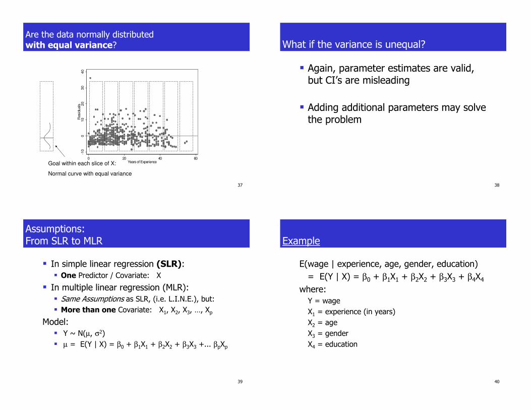
Are the data normally distributed with equal variance?

-10

01

02

03

04

0R

esid

uals

0 20 40 60Years of ExperienceGoal within each slice of X:

Normal curve with equal variance

38

What if the variance is unequal?

� Again, parameter estimates are valid, but CI’s are misleading

� Adding additional parameters may solve the problem

39

Assumptions:From SLR to MLR

� In simple linear regression (SLR):� One Predictor / Covariate: X

� In multiple linear regression (MLR):� Same Assumptions as SLR, (i.e. L.I.N.E.), but:

� More than one Covariate: X1, X2, X3, …, Xp

Model:� Y ~ N(µ, σ2)

� µ = E(Y | X) = β0 + β1X1 + β2X2 + β3X3 +... βpXp

40

Example

E(wage | experience, age, gender, education)

= E(Y | X) = β0 + β1X1 + β2X2 + β3X3 + β4X4

where: Y = wage

X1 = experience (in years)

X2 = age

X3 = gender

X4 = education

41

Assessing assumptions with multiple continuous X’s

� Residual plot is usually vs. fitted values� if problems, then plot against each X

� Can’t assess model by plotting Y vs. X� plot shows unadjusted relationship

� model shows relationship adjusted for other X’s

� Use AV plot instead � shows the relationship between Y and X after

adjusting for the other X’s

42

Lecture 10 Summary

� Linear regression assumptions

� L assess with Y vs. X (AV plot)

� I cannot assess

� N assess with Y vs. X (AVplot), residual plot

� E assess with Y vs. X (AVplot), residual plot

� Check assumptions for final model

� may have to continue modeling based on results

General approach for most statistical modeling: Lecture 10 ...eckel/biostat2/notes/notes10.pdf ·...

Documents

Transcript of General approach for most statistical modeling: Lecture 10 ...eckel/biostat2/notes/notes10.pdf ·...