Gene Structure & Gene Finding Part II · Repetitive DNA • Highly Repetitive DNA – Minisatellite...
31
Transcript of Gene Structure & Gene Finding Part II · Repetitive DNA • Highly Repetitive DNA – Minisatellite...
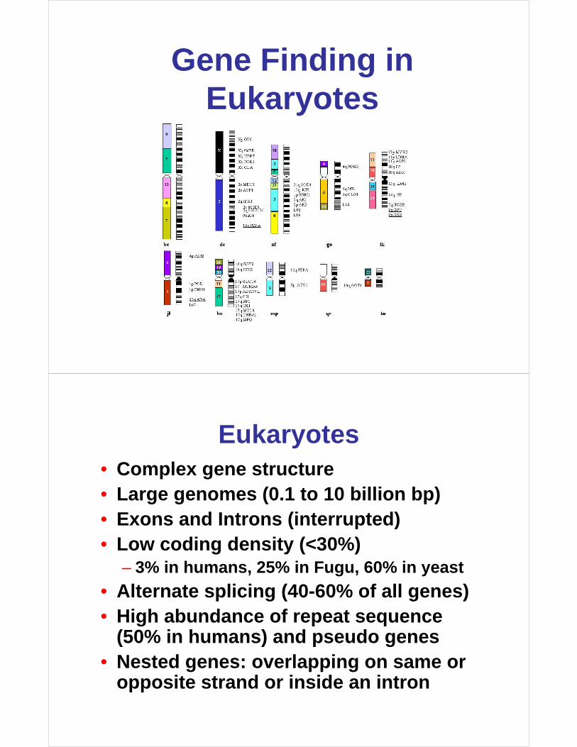
Gene Finding in Eukaryotes
Eukaryotes• Complex gene structure• Large genomes (0.1 to 10 billion bp)• Exons and Introns (interrupted)• Low coding density (<30%)
– 3% in humans, 25% in Fugu, 60% in yeast
• Alternate splicing (40-60% of all genes)• High abundance of repeat sequence
(50% in humans) and pseudo genes• Nested genes: overlapping on same or
opposite strand or inside an intron

Eukaryotic Gene Structure
exon 1 intron 1 exon 2 intron 2 exon3exon 1 intron 1 exon 2 intron 2 exon3
Transcribed RegionTranscribed Region
Start Start codoncodonStop Stop codoncodon
5’ UTR5’ UTR3’ UTR3’ UTR
UpstreamUpstreamIntergenicIntergenicRegionRegion
DownstreamDownstreamIntergenicIntergenicRegionRegion
5’site5’site 3’site3’site
branchpoint sitebranchpoint site
exon 1 intron 1 exon 2 intron 2exon 1 intron 1 exon 2 intron 2
AG/GTAG/GT CAG/NTCAG/NT
Eukaryotic Gene Structure

RNA Splicing
Exon/Intron Structure (Detail)
ATGCTGTTAGGTGG...GCAGATCGATTGAC
Exon 1 Intron 1 Exon 2
ATGCTGTTAGATCGATTGAC
SPLICE

Intron Phase
• A codon can be interrupted by an intron in one of three places
ATGATTGTCAG…CAGTAC
ATGATGTCAG…CAGTTAC
ATGAGTCAG…CAGTTTAC
AGTATTTAC
SPLICE
Phase 0:
Phase 1:
Phase 2:
Repetitive DNA
• Moderately Repetitive DNA– Tandem gene families (250 copies of rRNA,
500-1000 tRNA gene copies)
– Pseudogenes (dead genes)
– Short interspersed elements (SINEs)• 200-300 bp long, 100,000+ copies, scattered
• Alu repeats are good examples
– Long interspersed elements (LINEs)• 1000-5000 bp long
• 10 - 10,000 copies per genome

Repetitive DNA
• Highly Repetitive DNA– Minisatellite DNA
• repeats of 14-500 bp stretching for ~2 kb
• many different types scattered thru genome
– Microsatellite DNA• repeats of 5-13 bp stretching for 100’s of kb
• mostly found around centromere
– Telomeres• highly conserved 6 bp repeat (TTAGGG)
• 250-1000 repeats at end of each chromosome
Key Eukaryotic Gene Signals
• Pol II RNA promoter elements– Cap and CCAAT region
– GC and TATA region
• Kozak sequence (Ribosome binding site-RBS)
• Splice donor, acceptor and lariat signals
• Termination signal
• Polyadenylation signal

Pol II Promoter Elements
GC box~200 bp
CCAAT box~100 bp
TATA box~30 bp
Gene
Transcriptionstart site (TSS)
Exon Intron Exon
Pol II Promoter Elements
• Cap Region/Signal– n C A G T n G
• TATA box (~ 25 bp upstream)– T A T A A A n G C C C
• CCAAT box (~100 bp upstream)– T A G C C A A T G
• GC box (~200 bp upstream)– A T A G G C G nGA

Pol II Promoter Elements
TATA box is found in ~70% of promoters
WebLogos
http://www.bio.cam.ac.uk/cgi-bin/seqlogo/logo.cgi

Kozak (RBS) Sequence
-7 -6 -5 -4 -3 -2 -1 0 1 2 3A G C C A C C A T G G
Splice Signals
AG/GTAG/GT CAG/NTCAG/NT
branchpoint sitebranchpoint site
exon 1 intron 1 exon 2exon 1 intron 1 exon 2
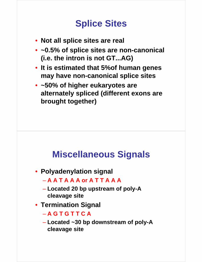
Splice Sites
• Not all splice sites are real
• ~0.5% of splice sites are non-canonical (i.e. the intron is not GT...AG)
• It is estimated that 5%of human genes may have non-canonical splice sites
• ~50% of higher eukaryotes are alternately spliced (different exons are brought together)
Miscellaneous Signals
• Polyadenylation signal– A A T A A A or A T T A A A
– Located 20 bp upstream of poly-A cleavage site
• Termination Signal– A G T G T T C A
– Located ~30 bp downstream of poly-A cleavage site

Polyadenylation
CPSF – Cleavage &PolyadenylationSpecificity Factor
PAP – Poly-A Polymerase
CTsF – CleavageStimulation Factor
Why Polyadenylation is Really Useful
AAAAAAAAAAA|||||||||||TTTTTTTTTTT
ComplementaryBase Pairing
Poly dTOligo bead
TTTT
TT
TT
TT
TT
TT
TT
TTTT
TT
TTT
AAAA
AA
AA

mRNA isolation
• • Cell or tissue sample is ground up and lysed with chemicals to release mRNA
• Oligo(dT) beads are added and incubated with mixture to allow A-T annealing
• Pull down beads with magnet and pull off mRNA
Making cDNA from mRNA
• cDNA (i.e. complementary DNA) is a single-stranded DNA segment whose sequence is complementary to that of messenger RNA (mRNA)
• Synthesized by reverse transcriptase

Reverse Transcriptase
Finding Eukaryotic Genes Experimentally
• Convert the spliced mRNA into cDNA
• Only expressed genes or expressed sequence tags (EST’s) are seen
• Saves on sequencing effort (97%)
CTGTACTAUACGAUAGACAUGAUAAAAAAAAAA
ATGCTAT Reverse transcriptase
mRNA
cDNA

Finding Eukaryotic Genes Computationally
• Content-based Methods– GC content, hexamer repeats, composition
statistics, codon frequencies
• Site-based Methods– donor sites, acceptor sites, promoter sites,
start/stop codons, polyA signals, lengths
• Comparative Methods– sequence homology, EST searches
• Combined Methods
Content-Based Methods
• CpG islands – High GC content in 5’ ends of genes
• Codon Bias– Some codons are strongly preferred in coding
regions, others are not
• Positional Bias– 3rd base tends to be G/C rich in coding regions
• Ficketts Method– looks for unequal base composition in different
clusters of i, i+3, i+6 bases - TestCode graph
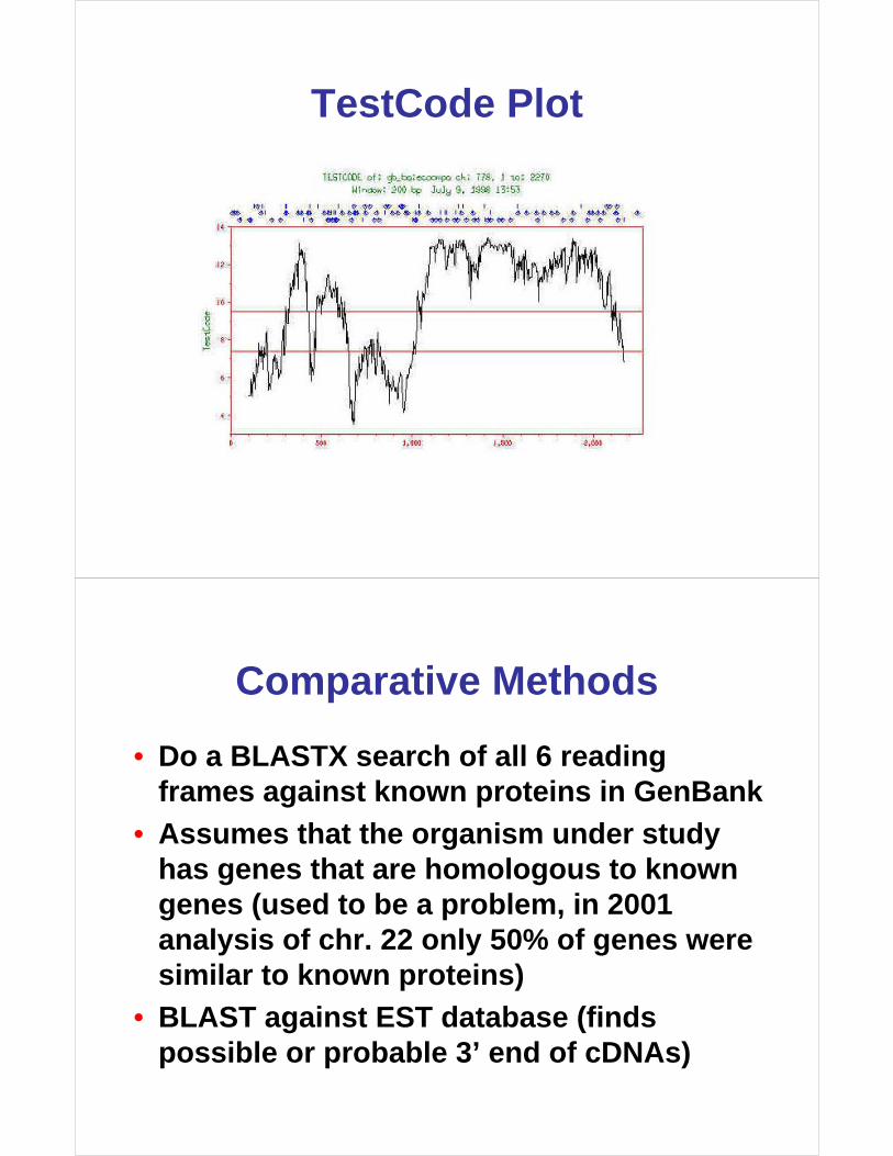
TestCode Plot
Comparative Methods
• Do a BLASTX search of all 6 reading frames against known proteins in GenBank
• Assumes that the organism under study has genes that are homologous to known genes (used to be a problem, in 2001 analysis of chr. 22 only 50% of genes were similar to known proteins)
• BLAST against EST database (finds possible or probable 3’ end of cDNAs)

BLASTX
Site-Based Methods
• Based on identifying gene signals (promoter elements, splice sites, start/stop codons, polyA sites, etc.)
• Wide range of methods– consensus sequences
– weight matrices
– neural networks
– decision trees
– hidden markov models (HMMs)

Neural Networks
• Automated method for classification or pattern recognition
• First described in detail in 1986
• Mimic the way the brain works
• Use Matrix Algebra in calculations
• Require “training” on validated data
• Garbage in = Garbage out
Neural Networks
Training Layer 1 Hidden OutputSet Layer
nodes

Neural Network Applications
• Used in Intron/Exon Finding
• Used in Secondary Structure Prediction
• Used in Membrane Helix Prediction
• Used in Phosphorylation Site Prediction
• Used in Glycosylation Site Prediction
• Used in Splice Site Prediction
• Used in Signal Peptide Recognition
Neural Network
ACGAAGAGGAAGAGCAAGACGAAAAGCAAC
ACGAAG
EEEENN
A = [001]C = [010]G = [100]
E = [01]N = [00]
DefinitionsTraining Set
Dersired Output
Sliding Window
[010100001]Input Vector
Output Vector[01]
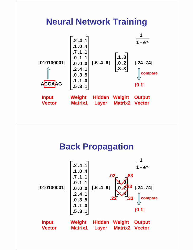
Neural Network Training
[010100001]
.2 .4 .1
.1 .0 .4
.7 .1 .1
.0 .1 .1
.0 .0 .0
.2 .4 .1
.0 .3 .5
.1 .1 .0
.5 .3 .1
[.6 .4 .6].1 .8.0 .2.3 .3
[.24 .74]
1
1 - e-x
Input Weight Hidden Weight OutputVector Matrix1 Layer Matrix2 Vector
compare
[0 1]ACGAAG
Back Propagation
[010100001]
.2 .4 .1
.1 .0 .4
.7 .1 .1
.0 .1 .1
.0 .0 .0
.2 .4 .1
.0 .3 .5
.1 .1 .0
.5 .3 .1
[.6 .4 .6].1 .8.0 .2.3 .3
[.24 .74]
1
1 - e-x
Input Weight Hidden Weight OutputVector Matrix1 Layer Matrix2 Vector
compare
[0 1]
.83
.33
.23
.22
.02

Calculate New Output
[010100001]
.1 .1 .1
.2 .0 .4
.7 .1 .1
.0 .1 .1
.0 .0 .0
.2 .2 .1
.0 .3 .5
.1 .3 .0
.5 .3 .3
[.7 .4 .7].02 .83.00 .23.22 .33
[.16 .91]
1
1 - e-x
Input Weight Hidden Weight OutputVector Matrix1 Layer Matrix2 Vector
Converged!
[0 1]
Train on Second Input Vector
[100001001]
.1 .1 .1
.2 .0 .4
.7 .1 .1
.0 .1 .1
.0 .0 .0
.2 .2 .1
.0 .3 .5
.1 .3 .0
.5 .3 .3
[.8 .6 .5].02 .83.00 .23.22 .33
[.12 .95]
1
1 - e-x
Input Weight Hidden Weight OutputVector Matrix1 Layer Matrix2 Vector
Compare
[0 1]ACGAAG

Back Propagation
[010100001] [.8 .6 .5] [.12 .95]
1
1 - e-x
Input Weight Hidden Weight OutputVector Matrix1 Layer Matrix2 Vector
compare
[0 1]
.84
.34.21
.01
.1 .1 .1
.2 .0 .4
.7 .1 .1
.0 .1 .1
.0 .0 .0
.2 .2 .1
.0 .3 .5
.1 .3 .0
.5 .3 .3
.02 .83
.00 .23
.22 .33.24
After Many Iterations….
Two “Generalized” Weight Matrices
.13 .08 .12
.24 .01 .45
.76 .01 .31
.06 .32 .14
.03 .11 .23
.21 .21 .51
.10 .33 .85
.12 .34 .09
.51 .31 .33
.03 .93
.01 .24
.12 .23

Neural Networks
Input Layer 1 Hidden OutputLayer
ACGAGG EEEENN
Matrix1
Matrix2
New pattern Prediction
HMM for Gene Finding

Combined Methods
• Bring 2 or more methods together (usually site detection + composition)
• GRAIL (http://compbio.ornl.gov/Grail-1.3/)
• FGENEH (http://genomic.sanger.ac.uk/gf/gf.shtml)
• HMMgene (http://www.cbs.dtu.dk/services/HMMgene/)
• GENSCAN(http://genes.mit.edu/GENSCAN.html)
• Gene Parser (http://beagle.colorado.edu/~eesnyder/GeneParser.html)
• GRPL (GeneTool/BioTools)
Genscan

How Do They Work?
• GENSCAN– 5th order Hidden Markov Model
– Hexamer composition statistics of exonsvs. introns
– Exon/intron length distributions
– Scan of promoter and polyA signals
– Weight matrices of 5’ splice signals and start codon region (12 bp)
– Uses dynamic programming to optimize gene model using above data
How Well Do They Do?
Co
rrel
atio
n (
x100
)C
orr
elat
ion
(x1
00)
MethodMethod
61 63
7276
8694 97
0.0
10.0
20.0
30.0
40.0
50.0
60.0
70.0
80.0
90.0
100.0
Xpound GeneID GRAIL 2 Genie GeneP3 RPL RPL+
Burset & Guigio test set (1996)

How Well Do They Do?
"Evaluation of gene finding programs" S. Rogic, A. K. Mackworthand B. F. F. Ouellette. Genome Research, 11: 817-832 (2001).
Easy vs. Hard Predictions
3 equally abundant states (easy)BUT random prediction = 33% correct
Rare events, unequal distribution (hard)BUT “biased” random prediction = 90% correct

Gene Prediction (Evaluation)TP FP TN FN TP FN TN
Actual
Predicted
Sensitivity Measure of the % of false negative results (sn = 0.996 means 0.4% false negatives)
Specificity Measure of the % of false positive results
Precision Measure of the % positive results
Correlation Combined measure of sensitivity and specificity
TP FP TN FN TP FN TN
Actual
Predicted
Sensitivity or Recall Sn=TP/(TP + FN)
Specificity Sp=TN/(TN + FP)
Precision Pr=TP/(TP + FP)
Correlation
CC=(TP*TN-FP*FN)/[(TP+FP)(TN+FN)(TP+FN)(TN+FP)]0.5
Gene Prediction (Evaluation)
This is a better way of evaluating

Different Strokes for Different Folks
• Precision and specificity statistics favor conservative predictors that make no prediction when there is doubt about the correctness of a prediction, while the sensitivity (recall) statistic favors liberal predictors that make a prediction if there is a chance of success.
• Information retrieval papers report precision and recall,while bioinformaticspapers tend to report specificity and sensitivity.
Gene Prediction Accuracy at the Exon Level
Actual
Predicted
WRONGEXON
CORRECTEXON
MISSINGEXON
Sn =Sensitivitynumber of correct exons
number of actual exons
Sp =Specificitynumber of correct exons
number of predicted exons

Better Approaches Are Emerging...
• Programs that combine site, comparative and composition (3 in 1)– GenomeScan, FGENESH++, Twinscan
• Programs that use synteny between organisms– ROSETTA, SLAM, SGP
• Programs that combine predictions from multiple predictors– GeneComber, DIGIT
GenomeScan -http://genes.mit.edu/genomescan.html

TwinScan -http://genes.cs.wustl.edu/
SLAM -http://baboon.math.berkeley.edu/~syntenic/slam.html

GeneComber -http://www.bioinformatics.ubc.ca/genecomber/
submit.php
Outstanding Issues
• Most Gene finders don’t handle UTRs(untranslated regions)
• ~40% of human genes have non-coding 1st exons (UTRs)
• Most gene finders don’t’ handle alternative splicing
• Most gene finders don’t handle overlapping or nested genes
• Most can’t find non-protein genes (tRNAs)

Bottom Line...
• Gene finding in eukaryotes is not yet a “solved” problem
• Accuracy of the best methods approaches 80% at the exon level (90% at the nucleotide level) in coding-rich regions (much lower for whole genomes)
• Gene predictions should always be verified by other means (cDNAsequencing, BLAST search, Mass spec.)