Gender Discrimination and Efficiency in Marriage:

the Bargaining Family under Scrutiny

Helmut Rainer∗

The University of Essex

November 2004

Abstract

This paper criticizes the view that discrimination limits the disadvantagedsex to undertaking housework and thus ensures that gains from specializa-tion at the household level are not wasted. Our framework gives attention tocausal links between labor market discrimination and the strategic behaviorof women and men within families. We consider a repeated family bargainingmodel that links the topics of employment and households. A key aspect ofthe model is that marital bargaining power is determined endogenously: theamount of money a person earns—in comparison with a partner’s income—establishes relative marital bargaining power. Gender discrimination can alterhousehold behavior in surprising and sometimes unfortunate ways. We showthat: (i) the efficiency of household decisions is sometimes inversely related tothe prevailing degree of gender discrimination in labor markets; (ii) discrimi-nated against females have difficulty enforcing cooperative household outcomessince they may be extremely limited to credibly punish opportunistic behaviorby their male partners; (iii) the likelihood that sharing rules such as “equalsharing” are maintained throughout a marriage relationship is highest whenmen and women face equal opportunities in labor markets. A key policy im-plication obtained from our analysis is that efforts to promote greater genderequality in labor markets can also contribute to increasing the likelihood offully cooperative outcomes at the household level.

Keywords: Gender Roles, Discrimination, Marital Negotiations, Rep-utation.

JEL Classifications: D13, J71, J82, C78.

∗Address for Correspondence: Department of Economics, University of Essex, Wivenhoe Park,Colchester CO4 3SQ, United Kingdom. E-mail: hraine@essex.ac.uk. I thank Abhinay Muthoo,Marco Francesconi, Antonio Nicolo, and seminar participants at the University of Essex for manyvaluable comments and suggestions. All errors are my own.

1

“Would it ever be optimal for a welfare-maximizing government, to wish to

end discrimination? ... By restricting access to good jobs, a discrimination

equilibrium limits the discriminated against sex to undertaking housework ...

and thus ensures that household-specific human capital is not wasted.” [Patrick

Francois, Journal of Public Economics, 1998].

“...two persons of cultivated faculties, identical in opinions and purposes, be-

tween whom there exists that best of equality, similarity of powers and capac-

ities ...This and this only is the ideal of marriage; ... all opinions, customs

and institutions which favor any other notion of it ... are relics of primitive

barbarism.” [John Stuart Mill, The Subjection of Women, 1869].

1 Introduction

Although equality between women and men has been firmly recognized as a pri-ority issue by the world’s governments,1 concerns about biased work practices andpublic policies are still raised at different levels. Differential wages and paymentrates constitute one important part of gender discrimination in most societies, andthere are many other spheres of differential benefits. For example, in opportunitiesfor promotion and achievement;2 in institutional characteristics of the labor mar-ket such as liberties to enter certain employment arrangements; but also in publicpolicies such as the tax treatment of families.3 The situation today from a policypoint of view is thus a split one. On the one hand, fundamental antidiscrimina-tion principles embedded in equal employment opportunity laws (EEO’s) seek tocreate a framework within which women can compete with men on equal footing.On the other hand, EEO’s are still subject to vigorous debate over whether theirperceived benefits outweigh the associated regulatory and efficiency costs, with theconsequence that unequal outcomes are perpetuated.

The debates about existing policies against gender discrimination is a subset of abroader issue: Why does gender discrimination exist as an equilibrium phenomenonin competitive labor markets? Can we explain the persistence of discrimination asarising from inherent asymmetries between men and women? We enter this broaddebate with what we take to be an important issue. To begin, many economistscontend that women’s increased employment over the past few decade has reducedthe joint gain from marriage because when wives are employed there is less special-ization within families and such specialization increases joint gain (Becker et al.,

1See, for example, United Nations Human Development Report (1995).2For example, the ‘glass ceiling’ restricting women’s career and development prospects, in par-

ticular their seniority and responsibility, remains firmly in place (Blau and Ehrenberg, 1997); Inaddition, even if women are as likely as men to be promoted, they often find themselves at thebottom of the wage scale for the new grade (Booth et al., 2002).

3Joint taxation systems tax both family members at the same rate. That joint taxation may

lead to differential treatment of men and women—by lowering the tax rate of the high-earner whichoccurs at the expense of an increase in the marginal rate of the low-earner—is well understood.With individual taxation, the low-earner is taxed at a lower-rate than the high earner. For ainsightful discussion of tax systems across Europe and elsewhere see O’Donoghue and Sutherland(1998).

2

1977; Becker, 1991). Motivated by this thought-provoking argument, this paper ad-dresses the following questions: Is it in ‘society’s’ interest to sustain discriminationas a means of discouraging women from entering work and supporting the divisionof labor within families (and thus, presumably, ensuring that no household-specifichuman capital is wasted)? Or, can we theoretically account for the possibilitythat the ‘joint gain’ from marriage increases even as specialization decreases withinmarriage?

The purpose of this paper is to investigate the impact of labor market discrim-ination on the economic roles of women and men within families. In doing so, weprovide the first fully developed treatment of the claim that the full impact of gen-der discrimination also includes feedback effects on women’s and men’s strategicbehavior within the household. We show that an assessment of this continuous un-derlying feedback effect is a key aspect in the analysis and formulation of policies,programs and initiatives targeted at gender differences. There are, of course, manychannels through which gender-specific labor market trends may impinge on familydecision-making. The finer points of this paper focus on how gender discriminationaffects market and non-market decisions by women and men, intra-household bar-gaining, household distributional outcomes, and the degree of cooperation that canbe sustained within families.

To address these issues, we develop a repeated-game model of family bargain-ing that links household and labor market decisions. A key aspect of the one-shot(constituent) game is that marital bargaining power is determined endogenously:the amount of money a person earns—in comparison with a partner’s income—establishes relative bargaining power inside the family. This introduces a non-cooperative element to the couple’s decision-making problem since both partnersanticipate how their labor market decisions affect their marital bargaining powerand the share they can extract from family resources. This sets up a two-stagedecision problem. At the first stage each family member non-cooperatively choosesan investment in his or her individual earning power, while bargaining between thefamily members at stage 2 forms the basis of the allocation of time between labormarket work and contributions to a household public good. The investment deci-sion at stage 1 is to be interpreted broadly—for example, an ‘on-the-job’ effort ora career investment such as the commitment to work odd hours. It is shown that,introducing these dynamics result in strategic manoeuvreing by men and women,which traps the household in inefficient situations. There are two deviations fromthe first-best here: women’s and men’s participation in the world outside the familygives them power bases in family bargains based on income contributions. Antic-ipating this, they will overinvest in market activities in the first place. However,the personal gains (in terms of bargaining power) each family member makes byoverinvesting in market activities are apparently lost at the level of collective con-tributions to domestic public goods, which are chosen inefficiently low. Thus, in ourconstituent game, there is a separation between the incentives motivating individualfamily members and the rewards of collective cooperation.

Given the above observation, we examine how gender-specific labor markettrends affect investments, household public good provisions and welfare of a fam-ily in the equilibrium of the constituent game. Strikingly, in this environment,

3

gender discrimination in the labor market generally enhances aggregate householdoutcomes. The basic argument for this point runs as follows. If family publicgoods are under provided, then discrimination serves the role of imposing unequal(marginal) returns on individuals of opposite sex in order to reallocate their in-centives according to their comparative contribution efficiencies. The ‘gender gap’acts as a disincentive to work, pushes women towards greater specialization in thehousehold sphere, and supports traditional family arrangements. We show thattotal time contribution to the domestic public increases since the female devotesless time to the labor market. As a consequence, discrimination can be seen as aforce that shifts family decision-making closer to the first-best efficient householdequilibrium than it would be without discrimination.

It is also shown, however, that the one-shot interactions are characterized byan efficiency-equality trade off: subjecting women to greater inequality in the labormarket, which, in turn, implies less involvement with outside work and paid employ-ment, does tend to go with greater anti-female bias in intra-family distributions.In other words, the very presence of gender discrimination in the labor market mayresult in a ‘Kuznets effect’ at the micro level of intra-household resource allocations:households become better off; but better households become more unequal.

So, in the constituent game, gender discrimination is an exogenous force thatdeters socially costly but privately beneficial overinvestments in market activitiesor, put differently, it alleviates an collective action (or holdup) problem that arisesamong marital partners. However, when the spouses interact repeatedly over time,then the desirability of exogenous forces such as the “gender gap” does not onlydepend on the existence of a (socially costly) holdup problem within the family. Italso depends on the way informal agreements between spouses regarding maritalbehavior already address the holdup problem and the extent to which environmentalparameters would interfere with those informal agreements. In the second part ofthe paper, we therefore examine the repeated-game version of the constituent game.We are particularly interested in questions of when and how a couple can a achievean efficient household equilibrium in a self-enforcing manner. One way to do this isfor the family members to agree in advance to cooperate, with the efficient outcomebeing sustained by the threat that if one partner deviates then immediately ‘play’proceeds according to the inefficient constituent game.

A key issue that separates the constituent game from the repeated-game model iswhether environmental parameters (including wage and employment opportunitiesof each family member) matter for men’s and women’s incentives to cooperate. Oneof the fundamental insights that we obtain is that if the family members are identicalin every respect — that is, they have identical market and non-market skills andface equal opportunities in the labor market — then reputational forces are mostlikely to work: in such circumstances, the efficient outcome can be sustained forthe widest set of possible parameter values. However, if the family members aredifferent in some respects (e.g., if there is a ‘gender gap’ in pay or occupationalstatus), then there exists a conflict in the partners’ incentives cooperate. For,in such circumstances, the shifting balance of power within the family makes thedominant partner more likely to demand a renegotiation of the arrangement thatsustains the first-best after the marriage has begun.

4

What this suggests in the face of anti female-discrimination policy is the fol-lowing: whatever the consequences of such policy elsewhere in society, our modelpredicts that it will be successful in promoting more balanced power arrangementsinside families. This, in turn, implies that women’s and men’s incentives to coop-erate are at a medium level, rather than one’s being very strong but the other’sbeing very weak. Thus, efforts to promote greater gender equality in the labormarket can create the conditions for first-best efficient household equilibria to besustainable in the long-run, by essentially increasing the degree of cooperation thatcan be sustained within families. This result motivates a new perspective on familypolicy in general: a major factor in the policy-making process should be whetherpolicies targeted at families facilitate cooperation within households.

The remainder of this paper is organized as follows. The next section explainshow the paper relates to the literature. Section 3 lays down our baseline modeland studies its unique stationary subgame perfect equilibrium. The repeated gameis studied in Section 4. Section 5 discusses the implications of the theory. A briefconclusion is contained in Section 6.

2 Related Literature

This paper contributes to two literatures. As a contribution to the economics ofdiscrimination, it adds to the body of work investigating theoretically gender dis-crimination and its dimensions. Economists working in this area have generallyfocused on explaining the existence of gender discrimination in competitive labormarkets. Becker’s (1971) ‘taste-for-discrimination model’ describes discriminationas a preference for which the discriminator is willing to pay. Signalling theories(Rothschild and Stiglitz, 1982; Milgrom and Oster, 1987) explain discrimination asarising due to differences in the noise of productivity signals across gender. A finalbroad category of explanations arises from crowding theories of occupational segre-gation (Bergman, 1971; Arrow, 1973) which explore the consequences of confiningwomen to a limited number of occupations.4

Theoretically, our paper is new primarily in emphasizing two levels of integrationthat we have found missing in previous studies. First, we integrate the topics ofemployment and households, pointing to discrimination against women in labormarkets as affecting the division of labor at home and the way men and womenbehave on the job. Second, we provide a framework that gives attention to causallinks between the relative position of men and women in employment and intra-household bargaining and power arrangements. Interest in this area is explained bythe fact that an assessment of this continuous underlying feedback effect is a keyaspect in the analysis and formulation of policies, programs and initiatives targetedat gender differences. The papers most similar in spirit to ours are Iyigun andWalsh (2002) and Dessy and Pallage (2003). Iyigun and Walsh’s (2002) simulation

4More recently, Francois (1998), provides a rationale for the continued existence of genderdiscrimination which arises from the intra-household trade between men. This theory posits thatfirms can ensure that all of its employees are ‘non-shirkers’ if they do not have spouses in goodjobs. As a consequence, firms should reserve good jobs for males exclusively.

5

of a family behavior model predicts that empowering women through institutionalreform leads to lower fertility and higher educational attainment. Our frameworkis different from theirs, although some of the issues we are interested in are similar.Dessy and Pallage (2003) show that if women have a credible outside option tomarriage (such as the right to start their own business) then gender discriminationis likely to disappear.

Our approach to modelling discrimination envisions a discrimination coeffi-cient which measures social and cultural attitudes towards gender inequality. Thestrength of this coefficient reduces the ability of the discriminated group to trans-form market skills and market time into incremental earnings. This aspect of thetheory allows us to use nondiscrimination as a benchmark and to compare it withdiscriminatory labor market practices. The discrimination coefficient that we useto explain the feedback effect of sex discrimination on household outcomes is re-lated to Becker’s (1971) “taste-for-discrimination model” and to Iyigun and Walsh’s(2002) “endogenous household bargaining power model”. It should be emphasized,however, that, for the most part, the feedback effects to be discussed apply to otherprominent explanations of gender discrimination such as signalling-based theoriesor segmented labor market theories.

The paper also contributes to the theoretical literature on household behav-ior. The theoretical approach taken here can be seen as part of the ‘incomplete-contracting’ approach to modelling family behavior. This strand of research ex-plores the implications of the inability of family members to ‘commit across time’—inability which typically leads to inefficient household outcomes. Recent family be-havior models which have the feature of constraint efficiency include Konrad andLommerud (2000), Lundberg and Pollak (2001), Vagstad (2001), Basu (2001) andRainer (2003). The common feature of these models is that they set aside the rulingtradition in family economics that household are able to reach efficient outcomes.5

Konrad and Lommerud’s (2000) family behavior model is most closely relatedto the present one. There are, however, three important differences between thispaper and theirs. First, while Konrad and Lommerud (2000) focus on symmetricmarket and non-market decisions by males and females, a key point of the presentpaper is that these decisions may be asymmetric across gender. Second, this paperexplores in great detail the impact of gender-specific labor market trends on fam-ily welfare and household distributional outcomes. The third difference is that wespecify how family members can overcome inefficient situations and reach efficienthousehold resource allocations that are implicitly enforced through reputationalforces. Konrad and Lommerud (2000) instead propose a ‘static’ model in that thespouses are determining their relationship after one period. While the likely im-portance of reputational forces within households has been mentioned by numerous

5By contrast, most models of household behavior assume as a rule that families are able to reachefficient outcomes. For example, “the common preference approach” (Becker 1991), the “collectiveapproach” (Chiappori 1992; Chiappori et al. 2002) and Nash bargaining models of the family(Manser and Brown 1980; McElroy and Horney 1981; McElroy 1990) work with this assumption.For an insightful survey see Lundberg and Pollak (1996).

6

authors,6 the theoretical argument has not previously been developed.7 Hence, thepresent paper could be viewed as a way of reconciling family models of constraintefficiency and models of the household that merely assume efficiency.

3 The Model

In this section we present a simple model of a dual-breadwinner household. Thehousehold is comprised of two decision-makers, one male (m) and one female ( f).Time is divided into an infinite number of periods t = 1, 2, ...,∞. In each period, thehousehold resource allocation is made in two stages. We will refer to this two-stagegame as the constituent game. In the first stage, each family member invests in hisor her individual earning power, anticipating the impact this decision will have onthe intra-household balance of power. In the second stage, the couple determinethe allocation of time to household production through bargaining. Market workproduces a pure private good for each person, whereas time spent at home producesa pure household public good. We have chosen the pure private good—pure publicgood formulation as a benchmark. We now present the specific assumptions in eachstage of the base model.

A. Timing of the Constituent Game

Individuals must be proactive to be ‘successful’ in the labor market. At the be-ginning of stage 1 each agent of gender i, i ∈ {f, m}, simultaneously and non-cooperatively chooses an investment in his or her individual earning power. Thisinvestment is to be interpreted broadly—it could be, for example, a career invest-ment such as the commitment to work odd hours and not taking leaves in connectionwith household duties. We model agent i’s career investment as a continuous deci-sion: let wi ∈ [0, w] denote the investment of agent i. The cost to agent i of puttingin effort wi at work is measured by a strictly increasing and strictly convex costfunction β(wi). After choice of his or her career strategy, agent i’s labor marketwage rate is equal to wi. We assume that agents choose their career strategies byanticipating the impact this decision will have in the bargaining stage, in particularon the relative bargaining positions inside the household.

At the beginning of stage 2, the career investments wf and wm are observedby the individuals, and the couple bargain over the levels of their time contributionsto the household public good gf and gm, respectively. The amount of the householdpublic good is public in the sense that the payoffs that it generates are non-rivaland non-excludable. In each period, both agents are endowed with one unit oftime, gi ∈ [0, 1], which they allocate between market work and providing a home-produced family good. The family good that we have in mind is the time spentcaring for children. The psychic cost attached to such a time contribution is bi(gi).

6See, for example, Becker (1991), Konrad and Lommerud (1995), Lundberg (2002), and Rainer(2003).

7A notable exeption is the paper by Bernheim and Stark (1988). Using a repeated model ofmarriage, they criticize the view that altruism improves the allocation of resources within thefamily.

7

As in Lundberg and Pollak (1993) and Konrad and Lommerud (2000), we adoptthe Nash bargaining solution to describe the outcome of the bargaining process atstage 2, in which the “fall-back” position comprises a non-cooperative contributionequilibrium at that stage.

Our dynamic model represents the infinite repetition of the two-stage gameoutlined above. We adopt the simplifying assumption that career efforts as wellas contributions at home fully depreciate before the next period begins. Whilepotentially restrictive, it allows to focus on a model that is already sufficiently rich.

B. Preferences

Firms buy a package of time and effort from each individual, with payment tiedto the package rather than rendered separately for units of time and effort. Thehousehold public good is produced with a constant returns technology, i.e., outputof a domestic good is proportional to time input. Agents derive utility from apurely private good and from a household public good. As will be now seen, theterm ‘gender’ in our model refers to the home productivities and labor marketopportunities associated with being male and female. The payoff function of agenti is:

ui = θiwi(1 − gi) + G − γib(gi) − β(wi), for i ∈ {f, m} (1)

We would like to elaborate on this payoff formulation. The first term in the aboveequation reflects individual earnings implied by career effort wi and time spent atwork 1 − gi. We refer to the parameter θi in more detail below. The second termrepresents the amount of a household public good:

G = gf + gm.

Each agent i directly chooses his or her time contribution gi, the cost of which iscaptured by b(gi). We assume that b (gi) is strictly increasing and strictly convex ingi, that is, b′ (gi) > 0 and b′′ (gi). We further assume that women and men can havedifferent (psychic) costs of providing the public good, measured by the individual-specific parameter γi, with the resulting contribution cost γib (gi). The parameterγi reflects i’s contribution productivity at home: family members i’s capacity tocontribute to the household good (childcare) is high when both total and marginalcost (as captured by γi) for any level of time input is low. A first major aspectof our analysis is to entertain intrinsic differences between the sexes’ contributionproductivities.

Assumption 1 γf < γm.

Analytically, the assumption implies that women have a (possibly small) com-parative advantage in home production over men.8 The distinguishing feature of

8There exists a strong biological basis for this assumption. Our specification captures the ideathat women have a relatively strong commitment to the care of children because they want theirheavy biological investment in production up until birth to be worthwhile (Triver, 1972, Wright,1994). Men are typically less biologically committed to the care of children (Becker, 1991). It is wellunderstood that these biological differences lead to a comparative advantage between the sexes inthe care of children, and perhaps also in other household commodities (due to the complementaritybetween rearing children and other types of time use in the household sphere).

8

the analysis presented below is to provide a rationale for gender discrimination todisappear despite inherent differences in comparative advantage between the sexes..

C. The Discrimination Coefficient

A second major aspect of the model under study is that we aim to examine the feed-back effects of gender discrimination on household behavior. We do not attempt toidentify which of the potential causes of discrimination is most relevant, nor do wetake a stand on its microeconomic underpinnings. Instead, we introduce the exoge-nous coefficients θf and θm to capture the potential asymmetric opportunities ofmen and women in the outside labor market, where (θf , θm) ∈ [0, 1]2.9 In the casewhere θf = θm, the labor market opportunities of men and women are the same,10

which we will refer to as the non-discrimination benchmark. We characterize genderdiscrimination as a pair of infinitesimal changes in θf and θm in opposite propor-tional directions. Thus we capture the fact that the term “gender discrimination” inordinary usage conflates two mutually connected aspects: negative versus positivediscrimination. Indeed, in our analysis, not only do females suffer directly from dis-criminatory labor market practices, but such practices make the non-discriminatedgroup perform better economically relative to the non-discrimination benchmark.Since we consider an environment where gender discrimination affects the economicopportunities of men and women in opposite proportional directions, much can begained analytically by using the normalization θf ≡ θ and θm ≡ 1 − θ, wherean arbitrary value of θ over the interval [0, 1

2) is a measure of the propensity todiscriminate against women.11

We now solve the constituent game backwards, considering first the bargainingequilibrium at stage 2.

D. The Bargaining Equilibrium

We first derive the non-cooperative contribution equilibrium at stage 2. As inLundberg and Pollak (1993) and Konrad and Lommerud (2000), we will use thisoutcome to derive the NBS in which the non-cooperative equilibrium payoffs areconsidered to be the disagreement point. For an arbitrary set of career investments,(wf , wm), at stage 1, the non-cooperative contribution payoff to person i is givenby

di

(gni , gn

j

)= θiwi (1 − gn

i ) + gni + gn

j − γib (gni ) − β(wi), (2)

were (gni , gn

j ), i 6= j, are uniquely defined and solve the first order condition

θiwi + γib′ (gi) = 1 for i ∈ {f, m}. (3)

9An alternative interpretation is also applicable. One can also interpret θf and θm to be inversemeasures of the (potential asymmetric) cost of female and male participation in the labor market.

10Put differently, the rates of return on each level of effort and market time are the same formen and women

11Iyigun and Walsh (2002) use a similar concept in order to capture gender differences in the labormarket, interpreting the parameter θ as social and cultural attitudes towards gender inequality.

9

In the non-cooperative contribution equilibrium, the marginal private cost of spend-ing extra time at home must equal the marginal private benefit, which equals one.For future reference note that gn

i = gni (wi), that is, the allocation of time at stage

2 directly interacts with the allocation of effort at stage 1. At stage 2, the fam-ily members determine the allocation of time to household production, gf and gm

through bargaining. The non-cooperative contribution equilibrium is important indefining the disagreement payoffs in the stage 2 bargaining game.

We start by characterizing the husband-wife utility possibility frontier of theset of feasible payoff pairs that can be reached if an agreement is struck at stage 2.The Nash bargaining solution picks one point on this frontier. The husband-wifeutility possibility frontier, uf + um ≡ W is given by

W(gei , g

ej

)=

∑

i=f,m

θiwi (1 − gei ) + 2ge

i − γib (gei ) − β(wi), (4)

where (gei , g

ej ) are the maximizers of joint family welfare. They are uniquely defined

and solve the first order condition

θiwi + γib′ (gi) = 2 for i ∈ {f, m}. (5)

It is obvious that gei = ge

i (wi). Notice that the first order conditions for gni and

gei in (3) and (4), respectively, imply that, for an arbitrary wi chosen at stage 1,

gei > gn

i . That is, the non-cooperative contribution equilibrium at stage 2 suffersfrom underprovision of the domestic public good. Of course, this is due to the factthat the marginal private return from choosing gi (i.e., the right-hand side of (3))is less than the marginal social return from choosing gi (i.e., the right-hand side of(5)). As a consequence,

W (gei , g

ei ) > di(g

ni , gn

j ) + dj(gni , gn

j ),

implying that gains from cooperation at stage 2 do exist. Hence it is Pareto-efficientfor the couple to strike an agreement on how to allocate W (ge

i , gej ).

Applying the Nash bargaining solution with the non-cooperative contributionpayoffs in (2) as the “fall-back” position, the Nash bargained payoffs to f and mat stage 2 are determined by the split-the-difference rule:

uNi =

W (gei , g

ej ) + di(g

ni , gn

j ) − dj(gni , gn

j )

2, (6)

where gei = ge

i (wi) and gni = gn

i (wi). This says that each person first of all obtainsa payoff equal to the payoff that she/he obtains in the non-cooperative contribu-tion equilibrium–and then the remaining surplus from cooperation is split equallybetween the spouses.

E. Investment in Individual Earning Powers

Having solved the couple’s bargaining problem at stage 2 (for an arbitrary setof decisions made at stage 1) we next turn to their on-the-job effort decisions at

10

stage 1. As a benchmark, we first work out the first-best effort levels and theindividuals maximize joint surplus. The first-best efforts,

(we

i , wej

)∈ arg max

wi,wj

W(gei (wi), g

ej (wj)

),

are the unique maximizers of the ‘household welfare function’ in (4). It is straight-forward to establish that we

i uniquely solves the first-order condition

θi [1 − gei (wi)] = β′

i (wi) for i ∈ {f, m}. (7)

At the social optimum, the marginal social return from spending extra effort atwork must equal the marginal cost of that extra effort.

Consider next the equilibrium value of wi. Career investments wf and wm

are chosen simultaneously and non-cooperatively by f and m, respectively. Theequilibrium investment level,

wni = arg max

wi

uNi (ge

i (wi), gni (wi)) ,

is the unique maximizer of player i’s Nash-bargained payoff in (6). Define (gni )′ =

∂gni /∂wi. It is now straightforward to establish the following result:

Proposition 1 The constituent game has a unique subgame-perfect equilibrium.In this equilibrium, family member i (i = f, m) sets wi = wn

i , where wni is the

unique solution to the first-order condition

1

2

[θi [2 − ge

i (wi) − gni (wi)] − (gn

i )′]

= β′(wi). (8)

Equilibrium investments are chosen inefficiently high, that is wni > we

i . Further-more, equilibrium public good provisions are inefficiently low, ge (wn

i ) < ge (wei ) .

An efficient household resource allocation cannot be achieved.

Proof. See the Appendix.

There are two deviations from first-best here. The first inefficiency that is describedis the inefficiency of strategic over investment in individual earning powers. Themechanism that induces this excessive investment is a negative bargaining inter-nality: since the division of the gains from cooperation at stage 2 depend on theex post bargaining powers of the spouses, each spouse is led to put half weight onmaximizing his or her relative bargaining position (as captured by the differencedi − dj) when deciding on investments at stage 1. As a consequence, a “rat-race”equilibrium will result in which career investments are driven to a point where thesum of individual utilities is decreased. It is worth emphasizing that the secondtype of deviation from the first-best that is described here—inefficiently low con-tributions to the domestic public good—is due to wrong ex ante decisions, sincethe assumption of Nash bargaining at stage 2 ensures that there is no ex post inef-ficiency. In sum, the personal gains family members make by investing in marketactivities are apparently lost at the level of collective contributions to domesticgoods.

11

F. Returns to marriage through gender discrimination?

We are now ready to discuss the consequences of labor market discriminationagainst women on household behavior. We first investigate how a reduction ofwomen’s employment opportunities, relative to those of men, affects investments,time use, and welfare of a family in the subgame-perfect equilibrium of the con-stituent game. We then present comparative statics on the intra-household distri-bution of utility payoffs.

The feedback effect on aggregate household welfare. Since our aim isto examine the feedback effect of gender discrimination on men’s and women’sbehavior within the household, we use non-discrimination as a benchmark andcompare it to discriminatory labor market outcomes. Thus suppose that the statusquo in the labor market is full gender equity: θf = θm. That is, the rates of returnon each level of effort and market time are the same to women than to men. Wecharacterize gender discrimination as a pair of infinitesimal changes in θm and θf

in opposite proportional directions (as discussed in section 3.3). Now consider theimpact of a marginal decrease in θw and a marginal increase in θh on aggregatehousehold welfare. To derive this we take total differentials of the sum of the (Nashbargained) equilibrium utilities of all individuals in the household, using (6), andrecalling that wn

i = wni (θi), and ge

i = gei (wn

i , θi). The following general resultis useful in developing our subsequent analysis of the feedback effects of genderdiscrimination:

Lemma 1 Consider the case of discrimination for which dθf = −dθ < 0 < dθm =dθ, with female market opportunities reduced and male market opportunities raisedcompared to the non-discrimination benchmark. Then

dWN =

[wn

f

(1 − ge

f

)+

1

2

[θf

(gnf − ge

f

)+

(gnf

)′

] ∂wnf

∂θf

]dθf

+

[wn

m (1 − gem) +

1

2

[θm (gn

m − gem) + (gn

m)′] ∂wn

m

∂θm

]dθm. (9)

Proof. See the Appendix.

A pair of changes in θf and θm has four opposing effects on aggregate householdwelfare. We interpret the expressions in (9) term by term. The first term on theright-hand side of (9) represents the negative wage-income effect of female incomereduction induced by a marginal decrease in θf . The female wage income effectis negative precisely because a reduction in θf reduces f ’s marginal return fromputting in effort wn

f and time (1 − gef ) at work. On the other hand, the second

term on the right-hand side of (9), which is strictly positive, may be called thestrategic effect of a marginal reduction in θf ; it follows from the fact that a marginaldecrease in θf reduces f ’s incentive to strategically over invest in market activities(as discussed after Proposition 1). Indeed, the term 1

2 [θf (gnf − ge

f ) + (gnf )′], which

is negative, represents the exact value of the inefficiency that arises due to f ’sincentive to strategically over invest in market activities by choosing the privatelyoptimal wn

f rather than the socially optimal wei . Apart from reducing female full

12

income and reducing female incentives to behave strategically, discrimination hastwo additional effects: the third term on the right-hand side of (9), which is strictlypositive, represents the male wage-income effect, while the fourth term, which isstrictly negative, is the strategic effect of a marginal increase in θm; it follows fromthe fact that a marginal increase in θm further increases m’s incentive to behavestrategically inside the household compared to the non-discrimination benchmark.

To investigate the quantitative implications of those four opposing effects, wemake the following additional assumptions: We assume that the cost function b (gi)and β (wi) are quadratic, which is stated formally in the following:12

Assumption 2

γib(gi) =γi

2g2i and β(wi) =

1

2w2

i .

We further assume that γi

2 > 1, which ensures that interior solutions for all choicevariables exist. Under these assumptions, we first derive the counterpart of equation(9). After setting dθf = −dθ = −dθm (where dθ > 0), we obtain the followingresult:

Lemma 2 Given Assumption 2, the condition for the change in aggregate house-hold welfare is:

dWN

dθ

∣∣∣∣θ=θf=θm

=

θ(γf − 1

) (γ − γf

)(γf − θ

2)2

+

θ (γm − 1) (γm − γ)(γm − θ

2)2

, (10)

where γ = 3.

Proof. See the Appendix.

Recall that γf and γm (where γf < γm by Assumption 1) reflect the inverses ofthe family members’ contribution productivities at home, so that i’s contributionto the domestic public good is an important component of aggregate householdwelfare when γi is low and vice versa. The first term in brackets represents thesum of the negative (wage-income) effect of female full income reduction and thepositive (strategic) effect of reduced female incentives to strategically overinvest inmarket activities. Similarly, the second term in brackets captures the sum of themale wage-income effect (> 0) and the male strategic effect (< 0). The focus of thesubsequent discussion is on equation (10). The following result, which is exploredafter its statement, shows that there may be a close connection between women’semployment opportunities, relative to those of men, and aggregate household wel-fare.

12We make this assumption purely to simplify the exposition of some of our results, but, itshould emphasized, without affecting our main insights. Let us be more specific: the assumptionof quadratic cost functions guarantees that the third derivatives of b and β are zero. One cangenerally show that b′′′ = 0 and β′′′ = 0 are sufficient conditions under which the conclusionsstated in Proposition 2 holds. Weaker sufficient conditions — which, for example, allow for b′′′ > 0or b′′′ < 0 — exist under which the stated conclusion would also hold.

13

Proposition 2 Suppose that Assumptions 1 and 2 hold. Then gender discrimina-tion with female market opportunities reduced and male market opportunities raisedcompared to the non-discrimination benchmark increases aggregate household wel-fare.

Proof. See the Appendix.

Intuitively, the mechanism is the following. Consider first the scenario whereγf < γ < γm. In this case female contributions to the household public goodare an important component of aggregate household welfare, while male contribu-tions are relatively unproductive. The type of gender discrimination consideredhere is welfare-enhancing in its impact precisely because it reduces female incen-tives to strategically overinvest in market activities. This, in turn, shifts femalehousehold public good provisions closer to the first-best than they would be in thenon-discrimination benchmark. What is more, the chain reaction set in motion byreducing females incentives to overinvest in market activities results in offsettingthe negative effect of female full income reduction. To see this, simply note thatthe first-term in brackets in (10) will be strictly positive when γf < γ. The ex-act opposite will be true for men. Male incentives to strategically overinvest inmarket activities increase. This, in turn, reduces male household public good pro-visions even further. However, since male contributions are less productive thanfemale contributions, male underinvestment in the household sphere is much less ofa problem in terms of aggregate household welfare. In fact, when γ < γm, then thepositive male income effect dominates the negative strategic effect. To see, this notethat the second-term in (10) is strictly positive with the parameter values underconsideration.

Consider now the scenario where γf < γm < γ, that is, both female and malecontributions in the household sphere are an important component of householdwelfare. In this case, the first term in (10) is strictly positive while the second termis strictly negative. That is, the negative female wage-income effect is offset by thepositive female strategic effect, while the positive male wage-income is dominatedby the negative male strategic effect. It is easily verified that, on aggregate term, thefirst term strictly exceeds the second term.13 The intuitive reason for this resultis straightforward. The female (strategic) underprovision of the domestic goodthe subgame perfect equilibrium of the constituent is a more severe problem thanthe male underprovision because her investment is more productive. Consequently,given our assumption about domestic technology, a change in θf and θm in oppositeproportional directions will increase female domestic contributions by more thanit reduces male domestic provisions, thereby pushing aggregate household welfarecloser to the first-best outcome.

So, it has been shown that concerns about intra-household lead to over invest-ment in market activities, which, in turn, implies underprovision of domestic publicgoods. In such an environment, discrimination may be long lived precisely becauseit plays the role of imposing unequal (marginal) returns on individuals of opposite

13Note that, since we are using non-discrimination as a benchmark and compare it to discrimi-natory labor market outcomes, the equation (10) must be evaluated at θf = θm = θ.

14

-

6

θ ∈ [0, θ)

W (θ)

θ θ = 12

=

U

W (θ)

W (θ)

θ

(a) (b)

Figure 1: The relationship between aggregate household welfare and men’s andwomen’s relative opportunities outside the household.

sex, thereby reallocating their incentives according to their domestic contributionefficiencies: discrimination acts as an disincentive to invest in market activities,pushes women towards greater contributions in the domestic sphere, and thus sus-tains some of the gains from specialization according to comparative advantages.

The present analysis is limited to environments in which, relative to the non-discrimination benchmark, discriminatory practices affect the economic opportu-nities of women and men in opposite proportional directions. Some additionalintuitive insights can be gained by abusing previously used notation and normalizeθf = θ and θm = 1 − θ, where an arbitrary value of θ over the interval θ ∈ [0, θ)(where θ = θf = θm) is a measure of the society’s propensity to discriminateagainst women. Figure 1 plots aggregate household welfare W N against the coeffi-cient θ. Panel (a) depicts household welfare for an arbitrary θ ∈ [0, θ). Panel (b)depicts household welfare when men and women have equal opportunities outsidethe household, that is, when θf = θm = θ.

What is clear from the figure is that aggregate household welfare is a nonmono-tonic function of θ.14 Indeed there exist a critical value θ over the interval [0, θ)such that an intensification of the “gender gap” (as represented by a decrease in

14We should note that, given Assumption 2, aggregate household welfare is given by

WN =

θ2

f

(γ2

f − 1)

+ 4γf

(1 − θ2

f

)

2γf

(γf − θ2

f

) +θ2

m

(γ2

m − 1)

+ 4γm

(1 − θ2

m

)

2γm

(γm − θ2

m

)

where θf ≡ θ and θm ≡ 1−θ. Figure 1 depicts the case γf < γm < γ. We also note that W N is notnecessarily nonmonotonic in θ. Indeed, when the parameters are such that either γf < γ < γm or

γ < γf < γm, then W N is a strictly decreasing function over the interval [0, θ), with a maximum

at the corner θ = 0. In the case where γf < γ < γm, W N decreases at decreasing rates; when

γ < γf < γm, then W N decreases at increasing rates.

15

θ) increases welfare for all θ ∈ (θ, θ). While we do not propose to characterize thecritical value θ, some remarks on its structure worth making. In particular, it isreadily verified that the larger are the comparative advantages of women over menin terms of contributions in the domestic sphere, the smaller is the value of θ (andhence the larger the “gender gap”) at which household welfare is maximized.

The discussion thus far has focused on the relative positions men and womenoccupy within the labor market, and the consequences for aggregate household wel-fare. We have said little about the potential effect on intra-household distributions.We now turn to a closer examination of this issue.

The feedback effect on intra-household distributions. Proposition 2 im-plies that a welfare maximizing ‘society’ or ‘central planner’ may never wish to enddiscrimination as a way of supporting family arrangements with a sustained special-ization according to comparative advantages. So far, we have left it entirely openas to how gender discrimination in the labor market affects the final distributionof utilities within the household. An obvious measure of the final distribution ofutilities (i.e., of intra-household inequality) in this representative household is thedeviation from ‘equal shares’ of the female partner’s Nash bargained utility payoff:

I =uN

f

WN−

1

2=

1

2

[dN

f − dNm

WN

]. (11)

Changes in the final distribution of utilities will depend, therefore, on how changesin θw and θh affect total household welfare as captured by the household welfarefunction WN . In fact when household welfare increases then the final distributionof utilities between uN

f and uNm will, other things being equal, become more equal.

Similarly, when household welfare decreases then the final distribution of utilitiesbetween uN

f and uNm will, other things being equal, become more unequal. Of course,

other things are not equal and the disagreement payoffs dNf and dN

m (i.e., the relativebargaining positions within the household) will also change with changes in θf andθm. It this interaction which is of interest and which yields the following proposition.

Proposition 3 Labor discrimination against women does tend to go with greateranti-female bias in intra-family distributions:

2(duNf ) =

[wn

f

(2 − ge

f − gnf

)−

∂gnf

∂θf

]dθf−

[wn

m (gem − gn

m) − 2 (gnm)′

∂wnm

∂θm−

∂gnm

∂θm

]dθm < 0

and

2(duNm) =

[wn

m (2 − gem − gn

m) −∂gn

m

∂θm

]dθm−

[wn

f

(gef − gn

f

)− 2

(gnf

)′∂wn

f

∂θf

−∂gn

f

∂θf

]dθf > 0,

implying that the male partner is always better off and the female partner is alwaysworse off compared to the non-discrimination benchmark.

Proof. See the Appendix.

Discrimination has two opposing effects on the female partner’s Nash bargainedequilibrium payoff. On the one the hand, total household welfare increases (see

16

Propositions 2 and 3), the Pareto frontier shifts outwards, and the female partnerreaps half of that increase. On the other hand, gender discrimination in the labormarket affects marital bargaining power directly. The wife’s disagreement payoffdN

f decreases and the husbands disagreement payoff dNm increases. Therefore, the

inequality between dNm and dN

f increases, which, in turn, increases the inequality

between uNf and uN

m. The above result then implies that, on aggregate terms, thefemale partner’s bargaining position deteriorates by more than half the increasein household welfare. Hence, the persistence of discrimination can have seriousrepercussions for women by not only decreasing their opportunities and rewards inthe labor market but by also increasing intra-household inequality.

So, to summarize, when intra-household bargaining positions are determinedendogenously according to spousal incomes , then the power relationship in thefamily closely resembles the relative opportunities of men and women in the exist-ing stratification system of the labor market. Consequently discrimination againstwomen in the labor market goes hand-in-hand with an unbalanced distribution offamily power. We can thus expect that when women are excluded from attainingequal access to valued positions in the labor market, then inequality in equilibriumpayoffs at the household level will also persist. It should be also emphasized that thevery presence of gender discrimination in the labor market may result in a ‘Kuznetseffect’ at the micro level of intra-household allocations: households become betteroff because females are less likely to strategically overinvest in market activities;but better off households become more unequal.15

The results of the static model are interesting per se. If investments in individualearning powers are presumed to affect intra-household bargaining powers, our studydemonstrates that excessive incentives to invest in market activities will curtail thecouple’s present contributions to domestic public goods. In such an environment,discrimination is likely to be long-lived because it guarantees second-best householdarrangements and thus sustains the some of benefits that ‘society’ gains from thespecialization of men and women according to comparative advantages.

Yet, the baseline model lacks an important dimension of the reality of householdbehavior: we have described a ‘static’ model, in that the spouses are determiningtheir relationship after one period. Implicitly, therefore, we have been ignoringthe potential effects of reputation. This restrictive since it is often argued thatreputational forces can overcome many of the inefficiencies identified in the firsthalf of this paper. In the following section we explore the robustness of our resultsto such ‘dynamic’ considerations. In particular, we address the questions of whenand how a household may succeed in using its resources efficiently in a self-enforcingmanner.

4 Fully Cooperative Household Outcomes

In this part, we study the ability of family members to achieve efficient outcomeswhen the underlying family structures are sub-optimal. The key to our approach

15Kuznets (1955) posed the classic question as to whether inequality increases or decreases asthe economy grows.

17

is recognizing that when households are potentially trapped by strategic over in-vestments in market activities, then implicit informal agreements enforced throughrepeated interaction can protect family members against the resulting inefficientoutcome. As we mentioned below, while the likely importance of ‘reputationalforces’ within households has been mentioned by numerous authors, the theoret-ical argument has not previously been developed. The repeated-game version ofthe base model of Section 2 is well-suited to analyze implicit agreements betweenspouses enforced through reputational forces.

A. Efficient Household Equilibrium

Suppose the parties play repeatedly the constituent game described in the previoussection. We assume complete information, that is, at each decision node bothplayers can observe the entire back history of the game. Call Γ (δ) the resultingrepeated game with joint discount factor δ. Unlike in the constituent game, therepeated interactions among spouses may provide incentives to achieve and sustainan efficient household equilibrium (EHE, for short), provided the spouses valuetheir reputations sufficiently. The chore of our analysis is therefore deriving theincentive-compatibility conditions that are required to hold in order for there toexist an EHE in which, in each period, the Pareto-efficient outcome is reached andno strategic problems arise. We analyze grim-trigger-strategy equilibria, in whichthe EHE is sustained by moving play to the subgame-perfect equilibrium of theconstituent game if any spouse ever unilaterally deviates from the EHE path

There are, of course, several plausible manners in which the opportunity tosustain efficient outcomes can be interlaced within the structure of the constituentgame. We know turn to a description of one such ‘implicit agreement’ betweenspouses. Suppose that at the beginning of their relationship the spouses meetand agree not to behave strategically throughout their relationship. That is, theycommit themselves to choose (in each period t = 1, 2, ...,∞) the socially optimalwi = we

i and gi = gei (i = f, m) in order to maximize aggregate household welfare.

To support the efficient outcome on the equilibrium path of the repeated game,the spouses may need to split the surplus from cooperation in a different way thanin the constituent game. We assume that to split the gains from cooperation, thespouses also implicitly commit themselves to a per-period utility transfer t ∈ <from m to f (which can be positive or negative). The transfer will be determinedlater. If both spouses “honor” this implicit agreement and cooperate, then the per-period payoffs of the spouses along the EHE path are given by uE

f + t and uEm − t,

where

uEi = θiw

ei [1 − ge

i (wei )] +

[gef

(we

f

)+ ge

m (wem)

]− γib (ge

i (wei )) − βi (w

ei ) .

However, since an agreement on (wef , we

m, gef , ge

m) and t is not automatically enforce-

able,16 each spouse can choose whether or not to renege on his or her part of the

16This is precisely because the vector(we

f , wem, ge

f , gem

)and the transfer t do not constitute a

subgame-perfect equilibrium of the constituent game.

18

agreement at any of the two stages within each period: either at stage 1: either atstage 1 by choosing wi 6= we

i , or, at stage 2 by choosing not to make (or accept)the agreed transfer t. If any family member unilaterally violates the agreement,then immediately play proceeds according to the constituent game in Section 3. Inparticular, if family member i deviates at stage 1 by choosing wi 6= we

i , then thedivision of the marital surplus in that period would be determined by the partiesrespective disagreement points di and dj (as in the constituent game). That is,bargaining at stage 2 would result in the ‘split-the-difference’ rule. It thus followsimmediately that i’s deviation payoff is maximized by deviating at stage 1 andsetting wi = wn

i . Hence the deviation investment level at stage 1 is equal to theinvestment level in the constituent game. Family member i’s deviation payoff ofsetting wi = wn

i at stage 1 therefore equals

uDi =

WD + dNi − dB

j

2. (12)

For explicitness we have introduced some shortcut variables. The expression W D

represents joint family welfare when i behaves as unilateral defector, while j honorsthe implicit agreement.17 The expression dN

i represents the disagreement point ofthe spouse who behaves as a unilateral defector. (Note that the deviation disagree-ment point of i is equal to his or her disagreement point in the constituent game.18)Finally, dB

i represents the disagreement point of the “betrayed” spouse, that is, theone who honors the implicit agreement and chooses socially optimal actions at stage1.19

Since the EHE is not a subgame-perfect equilibrium of the constituent game,the EHE path can only be sustained by the threat of credible punishment if anyspouse ever unilaterally deviates from the EHE path. We assume that the partiessupport the EHE through grim-trigger strategies. That is, if any family unilaterallyviolates the EHE, then immediately his or her partner punishes this transgression byswitching play forever after to subgame-perfect equilibrium of the constituent game.Such punishment is credible in that each family member willingly participates inpunishment, given the other’s participation. Family member i’s payoff along the“punishment path” therefore equals his or her payoff in the constituent game:

uNi =

WN + dNi − dN

j

2. (13)

Again we are using shortcut variables: W N denotes joint family welfare in theconstituent game, while dN

i − dNj represents the relative bargaining positions along

the punishment path.

B. The Incentive-Compatibility Conditions

An efficient household equilibrium is self-enforcing if, in each period, family mem-ber i (i = f, m) sets wi = we

i at stage 1, sets gi = gei (w

ei ) at stage 2, and the agreed

17Therefore W D as in (4), but with gei replaced by ge

i (wni ) and ge

j replaced by gej = ge

j (wej ).

18Hence dNi is as in (2), but with gn

i replaced by gni (wn

i ).19Hence dB

i is as in (2), but with gni replaced by gn

i (wei ).

19

transfer t is implemented. Of course, the efficient outcome will be supported inequilibrium if and only if the discounted payoff stream from honoring the implicitagreement that sustains the EHE exceeds the discounted payoff stream from thedeviation-punishment path. It is straightforward to verify that the partners’ re-spective incentive constraints are given by

δ[(

uEf + t

)− uN

f

]≥ (1 − δ)

[uD

f −(uE

f + t)]

δ[(

uEm − t

)− uN

m

]≥ (1 − δ)

[uD

m −(uE

m − t)]

,

The left-hand side of each inequality represents the long-term average cost of devi-ating from the EHE path. This is because from next period onwards, f ’s per-period

loss would be(uF

f + t)− uN

f , while m’s per-period loss would be(uF

m − t)− uN

m.

The right-hand side of each inequality represents the short-term average benefitfrom the optimal deviation. Through straightforward manipulation of these twoinequalities, we obtain that agreed utility-transfer t is incentive-compatible if andonly if

t ≥ (1 − δ)[uD

f − uNf

]−

(uE

f − uNf

)(14)

t ≤(uE

m − uNm

)− (1 − δ)

[uD

m − uNf

]. (15)

These conditions are the parties’ incentive-compatibility conditions, which are re-quired to be satisfied in order for the EHE to be sustainable as a subgame-perfectequilibrium path. So far, we have been silent on the properties of the equilibriumtransfer t along the EHE path. We now turn our attention to this issue.

C. An Example of Possible Co-operation: “Equal Sharing”

How do husbands and wives plan to share in the spoils from cooperation? Thereare many possible scenarios, and our aim is not simply the demonstration thathousehold equilibria that generate efficient outcomes in the repeated game exist, butrather the exploration of descriptively interesting sharing rules that support efficientresource allocations in the long-term. We now construct an example of a bargaininggame in which the family members agree to implement, at the beginning of theirrelationship, a sharing rule that splits the gains from cooperation equally betweenthem. That is, we assume that the bargaining over the sharing rule at the outsetof marriage is such that the equilibrium negotiated transfer can be characterizedby the Nash bargaining solution with the disagreement point (0, 0). A naturalinterpretation of the repeated game model is thus implicit in its description: themodel captures an environment in which the probability that one person exertshis or her (bargaining) power over the other partner at the outset of marriageis negligible.20 Although we lack the direct evidence to make such an assertion,we strongly suspect that this captures a very realistic feature of life. Namely thestylized fact that the balance of power when a couple is first married is more or

20Farrell and Scotchmer (1988, p. 279), in their introductory discussion of partnerships, notethat “marriage is an equal sharing, and we avoid making spouses’ payoffs depend on their outsideopportunities.”

20

less equal, and then shifts in line with the individual’s access to resources suchas income or occupational status (see, for example, Hesse-Biber and Williamson,1984).21

The following alternative interpretation is also applicable: the model representsan environment in which the family members have a good sense, somehow sociallyand culturally derived, that equal sharing is a norm that supports mutually bene-ficial household outcomes; but also the fact that once this norm is violated familymembers will permanently enter into (costly) bargains in search of a new ‘sharingrule’ along the punishment path.

Given our assumption that the sharing rule t can be characterized by the Nashbargaining solution with disagreement point (0, 0), an application of NBS impliesthat the equilibrium negotiated sharing rules maximizes (uE

f + t)(uEm − t) subject

to (14) and (15). The following intermediate result is useful in developing oursubsequent analysis of an efficient household equilibrium with equal sharing:

Lemma 3 For each i = f, m, define

φi ≡[(1 − δi) uD

i + δiuNi

]. (16)

(a) If the parameter values are such that 12(uE

f + uEm) > max{φf , φm}, then the

equilibrium negotiated sharing rule is given by

tS =uE

m − uEf

2. (17)

(b) Otherwise, if the parameter values are such that 12(uE

f + uEm) ≤ max{φf , φm},

then the equilibrium negotiated sharing rule is a corner solution given by

tCo =

{uE

f − φf if 12(uE

f + uEm) ≤ φf

uEm − φm if 1

2(uEf + uE

m) ≤ φm

. (18)

Proof. Straightforward – hence omitted.

It is now straightforward (after substituting tS for t in (14) and (15), and sim-plifying) to derive the appropriate incentive-compatibility constraints under whichthe EHE with “equal sharing” can be sustained as a sub-game perfect equilibriumpath:

21It should be emphasized that no general consensus on how to determine the “sharing rule”in repeated hold-up problems has been reached in the literature. The “incomplete contractingapproach” (Halonen 2002) generally postulates a sharing that provides partners with balancedincentives to deviate from Pareto-efficient outcomes. It is however silent on whether the partnerswould agree in equilibrium to such a sharing rule. The “basic property rights approach” (Muthoo,2004) assumes that the equilibrium negotiated sharing rule can be characterized by the Nashbargaining solution, in which the disagreement point is given by the payoffs of the underlying(inefficient) constituent game. So other sharing rules than “equal sharing” are of course possible.But in general it seems descriptively most persuasive that marital partners plan to share the spoilsfrom cooperation fifty-fifty, but may have an incentive to renege on this sharing rule once themarital relationship is under way.

21

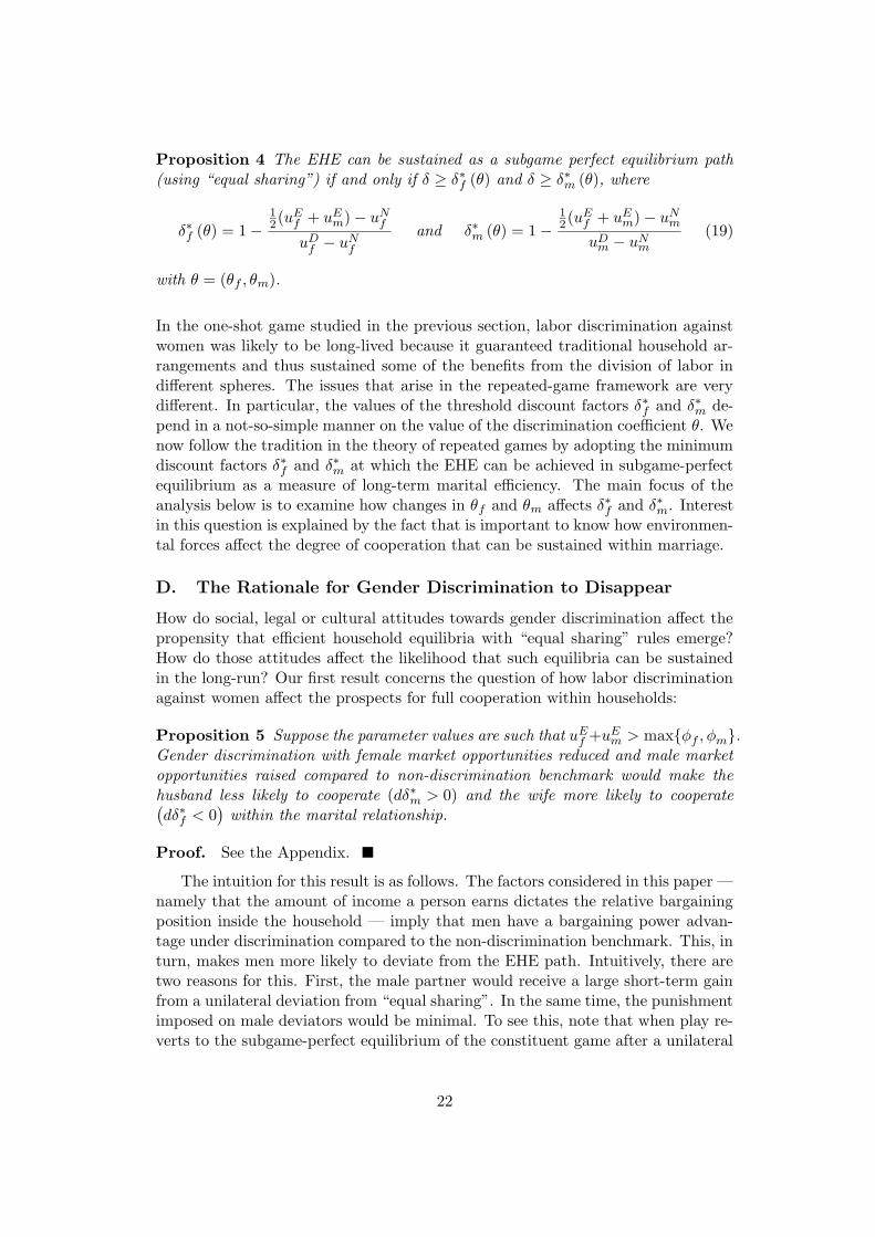
Proposition 4 The EHE can be sustained as a subgame perfect equilibrium path(using “equal sharing”) if and only if δ ≥ δ∗f (θ) and δ ≥ δ∗m (θ), where

δ∗f (θ) = 1 −12(uE

f + uEm) − uN

f

uDf − uN

f

and δ∗m (θ) = 1 −12(uE

f + uEm) − uN

m

uDm − uN

m

(19)

with θ = (θf , θm).

In the one-shot game studied in the previous section, labor discrimination againstwomen was likely to be long-lived because it guaranteed traditional household ar-rangements and thus sustained some of the benefits from the division of labor indifferent spheres. The issues that arise in the repeated-game framework are verydifferent. In particular, the values of the threshold discount factors δ∗f and δ∗m de-pend in a not-so-simple manner on the value of the discrimination coefficient θ. Wenow follow the tradition in the theory of repeated games by adopting the minimumdiscount factors δ∗f and δ∗m at which the EHE can be achieved in subgame-perfectequilibrium as a measure of long-term marital efficiency. The main focus of theanalysis below is to examine how changes in θf and θm affects δ∗f and δ∗m. Interestin this question is explained by the fact that is important to know how environmen-tal forces affect the degree of cooperation that can be sustained within marriage.

D. The Rationale for Gender Discrimination to Disappear

How do social, legal or cultural attitudes towards gender discrimination affect thepropensity that efficient household equilibria with “equal sharing” rules emerge?How do those attitudes affect the likelihood that such equilibria can be sustainedin the long-run? Our first result concerns the question of how labor discriminationagainst women affect the prospects for full cooperation within households:

Proposition 5 Suppose the parameter values are such that uEf +uE

m > max{φf , φm}.Gender discrimination with female market opportunities reduced and male marketopportunities raised compared to non-discrimination benchmark would make thehusband less likely to cooperate (dδ∗m > 0) and the wife more likely to cooperate(dδ∗f < 0

)within the marital relationship.

Proof. See the Appendix.

The intuition for this result is as follows. The factors considered in this paper —namely that the amount of income a person earns dictates the relative bargainingposition inside the household — imply that men have a bargaining power advan-tage under discrimination compared to the non-discrimination benchmark. This, inturn, makes men more likely to deviate from the EHE path. Intuitively, there aretwo reasons for this. First, the male partner would receive a large short-term gainfrom a unilateral deviation from “equal sharing”. In the same time, the punishmentimposed on male deviators would be minimal. To see this, note that when play re-verts to the subgame-perfect equilibrium of the constituent game after a unilateral

22

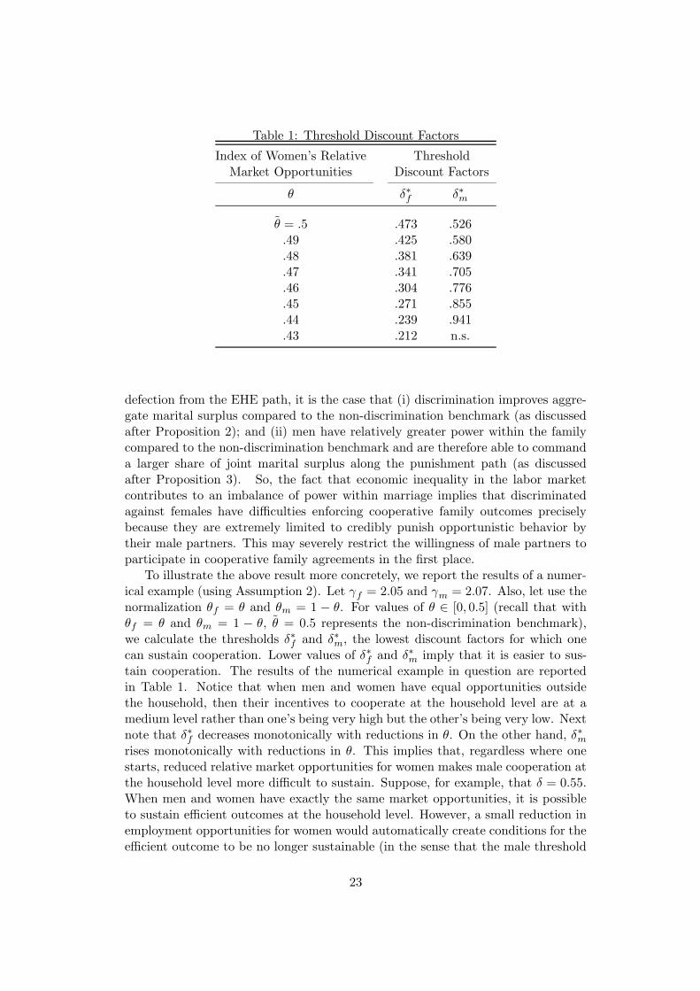
Table 1: Threshold Discount Factors

Index of Women’s Relative ThresholdMarket Opportunities Discount Factors

θ δ∗f δ∗m

θ = .5 .473 .526.49 .425 .580.48 .381 .639.47 .341 .705.46 .304 .776.45 .271 .855.44 .239 .941.43 .212 n.s.

defection from the EHE path, it is the case that (i) discrimination improves aggre-gate marital surplus compared to the non-discrimination benchmark (as discussedafter Proposition 2); and (ii) men have relatively greater power within the familycompared to the non-discrimination benchmark and are therefore able to commanda larger share of joint marital surplus along the punishment path (as discussedafter Proposition 3). So, the fact that economic inequality in the labor marketcontributes to an imbalance of power within marriage implies that discriminatedagainst females have difficulties enforcing cooperative family outcomes preciselybecause they are extremely limited to credibly punish opportunistic behavior bytheir male partners. This may severely restrict the willingness of male partners toparticipate in cooperative family agreements in the first place.

To illustrate the above result more concretely, we report the results of a numer-ical example (using Assumption 2). Let γf = 2.05 and γm = 2.07. Also, let use thenormalization θf = θ and θm = 1 − θ. For values of θ ∈ [0, 0.5] (recall that withθf = θ and θm = 1 − θ, θ = 0.5 represents the non-discrimination benchmark),we calculate the thresholds δ∗f and δ∗m, the lowest discount factors for which onecan sustain cooperation. Lower values of δ∗f and δ∗m imply that it is easier to sus-tain cooperation. The results of the numerical example in question are reportedin Table 1. Notice that when men and women have equal opportunities outsidethe household, then their incentives to cooperate at the household level are at amedium level rather than one’s being very high but the other’s being very low. Nextnote that δ∗f decreases monotonically with reductions in θ. On the other hand, δ∗mrises monotonically with reductions in θ. This implies that, regardless where onestarts, reduced relative market opportunities for women makes male cooperation atthe household level more difficult to sustain. Suppose, for example, that δ = 0.55.When men and women have exactly the same market opportunities, it is possibleto sustain efficient outcomes at the household level. However, a small reduction inemployment opportunities for women would automatically create conditions for theefficient outcome to be no longer sustainable (in the sense that the male threshold

23

discount factor δ∗m would be above the discount factor δ). On the other hand,suppose that δ = 0.8. In this case, an environment with large disparities in thelabor market (say with θ = 0.45) is inimical to emergence of efficient outcomesat the household level. However, a small expansion in employment opportunitiesfor women would translate into fully cooperative (and hence efficient) householdoutcomes.

Are there pointers for policy? Our analysis suggests that the reality of la-bor market discrimination against women assigns men and women assigns menand women to different roles within marital relationships. The resulting divisionof labor generates unequal bargaining positions within families because men canaccumulate resources (primarily earning power) which translates into a bargainingpower advantage. This male advantage makes it difficult for females to enforce fullycooperative (and hence efficient) outcomes at the household level. The immediate,main policy consequences are thus self-evident:

• If the labor market environment exhibits gender discrimination for women,and discount factors are such that the efficient household equilibrium (EHE)does initially not exist, then empowering women (through institutional orlegal reform) may create the conditions for the EHE to emerge and be sus-tainable in the long-run.

• If, on the other hand, discount factors are such that an efficient householdequilibrium does initially exist, then a small increase of gender differentialsin the labor market may create conditions for the EHE to be no longer sus-tainable.

Note that there are some additional insights that are implied by our numericalexample concerning the existence of parameter values under which there does notexist a subgame perfect equilibrium that sustains an efficient household equilibriumin which the spouses split the spoils from full cooperation equally. In particular,there exists a critical value θ ∈ [0, θ) (which lies between 0.43 and 0.44 in thecontext of the parameters used for the example) such that if θ ∈ [0, θ), then anefficient household equilibrium with “equal sharing” can never emerge in the long-run (i.e., not even in the limit as δ tends to one). The intuition is simple and followsfrom the fact when women’s relative market opportunities are below the thresholdθ, then the sharing rule tS that splits the gains from cooperation equally betweenthe spouses is not incentive compatible. More precisely, tS fails to satisfy the malepartner’s incentive constraint (15) in the sense that agreement to it would give hima utility level along the EHE path that is below what he could get from renegingon the agreement that sustains the EHE. This has to be viewed within the logicthat the male partner would loose out when the EHE is established since he wouldthen not be able to use his (large) bargaining power advantage to extract a largeshare of the marital surplus. In this case, the sharing rule is a corner solution andgiven by tCo = uE

m − φm (see Lemma 2b). The equilibrium payoffs are

um = φm and uf = uEf + uE

m − φm,

24

-

6

θ ∈ [0, θ)

W (θ)

θ θ = 12

W (θ)

U

W (θ)

/

Figure 2: Relationship between gains from marriage and men’s and women’s relativeopportunities outside the household in the repeated game.

where um > uf . As such, our main qualitative insights about intra-householdinequality — in particular, that labor discrimination against women triggers dif-ferences in equilibrium payoffs at the household level — is robust when the familymembers interact in a sequence of situations and can sustain the Pareto efficientoutcome.

We conclude this section by returning to one of the questions raised at theoutset of this paper. Can we theoretically account for the possibility that the gainsfrom marriage increase even as specialization within marriage decreases? Figure2 illustrates and summarizes our main insights, using the normalization θf = θand θm = 1 − θ. For a given discount factor δ, it plots aggregate family welfareagainst the discrimination coefficient θ. Recall that θ = θ describes an environmentwith equal opportunities for men and women outside the household, while θ < θcaptures an environment that disadvantages women and favors men. Also note thatthe coefficient θ not only measure the opportunities of women in the labor market,but it is also an index of the degree of specialization within households. This isexactly because a small value of θ provides little incentives for women to invest inmarket activities and large incentives to put available endowments to productiveuse in the household sphere. The figure clearly shows that aggregate family welfareis a discontinuous function of θ.22

For values of θ over the interval [0, θ), female face low opportunities outside thehousehold compared to men, and there exists a substantial degree of division of

22We have used the following numerical example to construct Figure 2. We let bi(gi) =γig2

i

2,

β(wi) =w2

i

2(i = f, m) , and (γm, γf ) = (2.4, 2.1) , so that there is difference in the spouses home

productivities, with the female partner having a comparative advantage. In addition, we considerdiscount factors δ ' 0.84. With this we have θ ≈ 0.5.

25

labor in the household. The household as a whole recaptures some of the advan-tages of the specialization of family members according to comparative advantages,but cooperation (and hence efficient household outcomes) do not emerge in a self-enforcing way. This is exactly because wives have little power in family bargains,and are consequently restricted to enforce efficient household equilibria becausethey are extremely limited to punish opportunistic behavior of their male partners.What is more, there is a anti-female bias in intra-family distribution (as discussedafter Proposition 3).

When θ equals θ, women have the same opportunities outside the householdas men. We note that there may still exist some degree of division of labor in thehousehold,23 but less extreme than before and less dependent on traditional sexroles. Put it differently, both spouses participate more equally in the market and inhousehold production. The implications for aggregate household welfare are verypowerful, the most notable feature being the sizeable increase in the gains frommarriage at θ. The increase in the gains from marriage arises in equilibrium pre-cisely because the better opportunities of women outside the household maintains abalance in the incentives to cooperate within the household. Put it differently, thegreater participation of women in the market gives them power in family bargainsbased on income contributions. This, in turn, gives them a means to punish op-portunistic behavior within households, and so limits the extent to which husbandshave an incentive to renege on efficient household equilibria with equal sharing. Insum, even if grant that specialization according to comparative advantages producesome joint gain in marriage, the above results suggest there is a countervailing forcewhich actually generates a larger joint gain when spouses play similar rather thandifferent “roles” both inside and outside marriage.

5 Discussion: The Relationship between Working and

Family Life

The model described above has a number of specific implications, some of whichwe have already discussed. In this section, we highlight the major points moregenerally and present empirical predictions that are relevant to some.

• Limits to specialization: the effects of reputation. Our findings are particu-larly interesting in the context of prior work, which has typically concluded thatthe specialization of family member according to comparative advantages wouldraise the gains from marriage. When family members have ‘common preferences’,Becker (1991) has argued that family members will specialize according to compar-ative advantages, not only regarding the division of labor, but also when it comesto human capital investments. Moreover, with common preferences, investments aswell as time will be allocated efficiently, i.e., so as to maximize joint family welfare.Becker’s (arguably powerful) approach ignores, however, the existence of so calledcooperative conflicts inside the family. The class of problems called ‘cooperativeconflicts’ generally acknowledges that in many social arrangements there are co-

23This is because females have a comparative advantage in home production (see Assumption2).

26

operative elements, but also elements of conflict in the choice of one arrangementrather than another.24 The existence of such cooperative conflicts within house-holds is now fully acknowledged by discussions of the bargaining problem insidethe family. Vagstad (2001) shows that even if real conflicts inside the family areaccounted for, different family members will continue to specialize according tocomparative advantages. However, the result that family decision-making is effi-cient does no longer hold: investments will be inefficient because they are chosenopportunistically so as to affect the outcome of the bargaining process itself.

Our family behavior model acknowledges the possibility of real conflicts of in-terests coexisting with an understanding of what is a natural way to overcome theinefficiencies due to ‘cooperative conflicts’. The key to our approach is recognizingthat reputational forces can alleviate many of the problems of opportunism iden-tified in static bargaining models of the family. One of the fundamental insightsthat we obtain is that if the family members are identical in every respect—thatis, they have identical market and non-market skills and face equal opportunities—then reputational forces are most likely to work. Indeed, in such circumstances, theefficient outcome (like in Becker’s framework) can be sustained for the widest setof possible parameter values. However, if the family members are different in somerespects (such as in their occupational status), then there exists a conflict in thepartners’ incentives to sustain the agreement that guarantees the efficient outcome.For, in such circumstances, the shifting balance of power within the family makesthe dominant partner (i.e., the one with power based on income contributions) morelikely to renege on his or her part of the agreement. Hence, where two membersof a household specialize completely in the market and household sector respec-tively, our study predicts that reputation is least likely to overcome the problemsof opportunism. And, without the influence of reputation, cooperation is unlikelyto be sustainable inside the family. This conclusion finds clear confirmation in theUnited Nations adoption of the Beijing Declaration and Platform for Action (1995)in which the ratifying countries declare that

“[E]qual rights, opportunities and access to resources, equal sharing ofresponsibilities for the family by men and women, and a harmoniouspartnership between them are critical to their well-being and that oftheir families as well as to the consolidation of democracy.”25

In contrast, ‘Beckerian’ theories of specialization emphasize the benefits that ‘soci-ety’ would gain from the division of labor in exclusively different spheres—and thusfail to provide a rationale for initiatives promoting equal responsibilities of womenand men in all sectors, including the family, the labor market and society at large.

• The balance of power inside the family closely resembles the position of menand women in the existing stratification system of the labor market. Marriage andfamily life is very much a matter of give and take. But who gives and who takes?Such issues are resolved by a process of negotiating and bargaining. Hence the con-cept of bargaining power is a key to understanding the interactions between different

24See Sen (1990) for an insightful characterization and analysis of co-operative conflicts.25See, for example, the OECD Development Assistant Committee (1998), Annex 2, Article 15,

p. 35.

27

members of the family. With the intra-household balance of power determined en-dogenously according to spousal incomes, the existence of gender discriminationin the labor market goes hand-in-hand with an unbalanced distribution of familypower. Thus, without equal access to pay and occupational status, women lack animportant tool in determining the allocation of household resources. From a distri-butional point of view one should be concerned, therefore, that the gender gap inthe labor market increases the differences in equilibrium payoffs at the householdlevel (as discussed after Proposition 3).

Why does this matter? Firstly, gender equality in all sectors is an importantgoal in itself—an issue of human rights and social justice (see, for example, UnitedNations Development Program, 1995). Secondly, the well-being of children — inparticular in the context of poor countries — is intrinsically bound up with thatof women: a certain amount of money given to the male partner and the sameamount given to the female can have very different effects on a child’s education,health, and the incidence of child labor (Basu, 2001). Thirdly, in many parts ofthe world, a neglect of the notion of ‘intra-household inequality’ is likely to lead toconsiderable understatement of the levels of inequality and poverty. In this regard,Haddad and Kanbur (1990) found underestimation by 30 percent and more in ananalysis of inequality in calorie intake on the basis of Philippine data set. Finally,sociologists have long emphasized that the failure to address gender inequalitieswithin households is significant because the family is the most influential institutionof social development. In this regard, households that operate according to powerarrangements based on gender differences are unlikely to be environments in whichto ‘unlearn’ norms of inequality (see, for example, Moller Okin, 1995).

While the above discussion is tailored to the context of developing countries,the problem of gender discrimination in the labor market can also have an effecton families in the economically advanced countries of Europe and North America.

• Gender-specific labor market trends and divorce rates: some speculations onthe empirical relationship. Marriage and family life provide a means of attainingspecific economic goals, and these relationships persist as long as both partnersexpect to be better off married than divorced (Becker et al., 1977).26 We can relaxour assumption that divorce is impossible and modify our model to allow for theprobability of divorce to be positive and endogenously determined by the level of“surplus” generated by that marriage (see, for example, Weiss and Willis,1985).Imagine first that divorce is the relevant threat point in the family bargain.27 Inaddition, let the spouses payoffs in marriage be ui + εi (rather than ui as in (1)),where the private gains from marriage, εi, are randomly drawn from a known

26Becker et al. (1977) demonstrate that the assertion that a couple will divorce each other onlyif it is efficient to do so is a special case of the Coase theorem (Coase, 1960).

27Konrad and Lommerud (2000) note that the predictions of using noncooperation as the dis-agreement point in the family bargain are similar to the case with utilities as single as the divorcethreat point. The difference between noncooperation and divorce is that the parties in the formercase still live together so the family public goods are still public goods. After a divorce some goodscease to be public goods, whereas others, as children, remain public goods. For the discussionto follow, let us interpret the disagreement points df and dm as the divorce threat points of theparties.

28

distribution and measure the quality of the marriage.28 It is straightforward toshow that the partners remain married if the total gains from marriage exceedthe total gains from divorce; i.e., when φ = (εf + εm) ≥ −(W − df − df ) whereW = uf + um captures the surplus generated by that marriage.

In such an environment, a marriage can remain intact either because the privategains from marriage, εi, are high, or because the surplus generated by that marriage,W , is high. The surplus generated is, of course, maximized when family-decisionmaking is efficient, i.e., when the first-best is implicitly enforced through repeatedinteraction. However, as we have shown in the preceding section, when family-decision making is efficient, then a small increase in the discrimination coefficientmay create conditions for the first-best to be no longer sustainable. For, in suchcircumstances, the shifting balance of power within the family makes the malepartner less likely to cooperate and more likely to renege the implicit agreementthat sustains the first-best. Thus, an increase in the discrimination coefficient mayshift family decision making from efficient to inefficient, inducing a fall in the surplusgenerated. Since a decrease in the surplus generated also decreases the gain fromstaying married compared to the gain from divorce, couples with an unbalanceddistribution of bargaining power are more likely to divorce.

Hence, there are good reasons to believe that women’s equal access to incomeand occupational status in the labor market is likely to reduce the probability ofdivorce, by essentially increasing the degree of cooperation that can be sustainedwithin the family. This conclusion goes counter to popular opinion that the in-creased labor force participation of married women in Western countries is respon-sible for much of the acceleration in divorce rates over the past four decades. Ingeneral, the framework discussed here provides a basis for understanding how twosignificant trends over the last few decade—the rise in divorce rates, and the gendergap in pay and occupational status—are correlated.

6 Concluding Remarks

This paper has explored the theoretical basis for the claim that the full impact ofgender discrimination also includes feedback effects on women’s and men’s strategicbehavior within the household. To understand this interaction theoretically it isnecessary to study it as a part of a model that links household and labor marketdecisions. Our findings are directly relevant to the literature on the economics ofthe family, in that they call into question the views mentioned at the outset ofthe paper. One should not necessarily expect that the efficiencies of specializationproduce a large joint gain in marriage, nor should gender discrimination be a con-structive social force that ensures that gains from specialization at the householdlevel are not wasted. Instead, our results suggest that the reality of labor market

28The sequence of events that we have in mind is as follows. In each period, at stage 1, eachpartner makes the investment into his or her individual earning power. At stage 1 1

2, each partner’s

private gain from marriage is realized, and the investment decisions are observed. At stage 2, if theyremain married, the partners bargain over time allocations and the surplus created by marriageover divorce. If they, divorce each spouse chooses his or her time allocation non-cooperatively.

29

discrimination against women assigns men and women to different roles within mar-ital relationships.The resulting division of labor generates unequal intra-householdbargaining positions because men accumulate resources (primarily earning power)which translate into a bargaining power advantage. This male advantage makesit very difficult to implement fully cooperative (and hence efficient) outcomes atthe household level, because women are severely restricted to credibly punish op-portunistic behavior by their male partners. Conversely, efforts to promote greatergender equality in labor markets lead to more balanced bargaining positions withinfamilies and thus increase the likelihood that the household remains an institutionthat is successful in allocating its resources efficiently.

7 Appendix

Proof of Proposition 1:

Differentiating uNi in (6) w.r.t wi yields

∂uNi

∂wi= θi(2−ge

i−gni )−

=0 by (5)︷ ︸︸ ︷[θiwi − 2g + γib

′

i (gei )

](ge

h)′−

=1 by (3)︷ ︸︸ ︷[θiwi + γib

′

i (gni )

](gn

i )′ = 2β′(wi)

where gei = ge

i (wi) and gni = gn

i (wi) with

(gei )

′ =∂ge

i

∂wi= −

θi

γib′′(ge

i )< 0 and (gn

i )′ =∂gn

i

∂wi= −

θi

γib′′(gn

i )< 0.

After using the first-order conditions in (3) and (5), we obtain condition (8) [whichis stated in the proposition]. We then note that the private marginal return ofchoosing wi is given by the left-hand side of (8):

rp ≡1

2

[θi [2 − ge

i (wi) − gni (wi)] − (gn

i )′].

Similarly, the social marginal return of choosing wi is given by the left-hand sideof (7):

rs ≡ θi [1 − gei (wi)] .

Differencing rp and rs one obtains

rp − rs =1

2

[θi(g

ei − gn

i ) − (gni )′

]> 0.

This term is strictly positive because gei > gn

i and (gni )′ < 0. Since the private

marginal return strictly exceeds the social marginal return, it follows that, at anyequilibrium at stage 1, the equilibrium market investments (wn

f , wnm) are strictly

above the joint surplus maximizing levels (wef , we

m). Furthermore, since gei is a

strictly decreasing function of wi, it follows that gei (wn

i ) < gei (we

i ).

Proof of Lemma 1:

30

Let the household welfare function be defined on the sum of (Nash bargained)utilities of the two family members. At the equilibrium of the constituent game wehave that

WN =∑

i=f,m

θiwni (1 − ge

i ) + 2gei − γibi (g

ei ) − β (wn

i ) , (20)

where gei = ge

i (wni , θi) and wn

i = wni (θi). Consider the case of discrimination for

which dθf = −dθ < 0 < dθ = dθm, with female market opportunities reduced andmale market opportunities raised compared to the non-discrimination benchmark.After totally differentiating W N , the expression for the change in household welfareis

dWN =

[wn

f

(1 − ge

f

)+

[θf

(1 − ge

f

)− β′

(wn

f

)] ∂wnf

∂θf

]dθf

+

[wn

m (1 − gem) +

[θm (1 − ge

m) − β′ (wnm)

] ∂wnm

∂θm

]dθm. (21)

After making use of (8) to substitute out β ′ (wni ) , expression (9) [which is stated

in the lemma] follows immediately.

Proof of Lemma 2:

Given Assumption 2, it is readily checked that the cooperative and non-cooperativepublic good contributions at stage 2 are respectively given by

gei = f

(2 − θiwi

γi

)=

2 − θiwi

γi

and gni = f

(1 − θiwi

γi

)=

1 − θiwi

γi

,

where f = (b′)−1. After substituting gei , gn

i and (gni )′ [which equals −θi/γi] into

(8) and setting β′ (wi) = wi one obtains

θi [(γi − 1) − θiwi] = γiwi.

It thus follows immediately that

wni =

θi (γi − 1)

γi − θ2i

(22)

and∂wn

i

∂θi=

(γi − 1)(γi + θ2

i

)

γi − θ2i

. (23)

We also note that

gei (wn

i ) =γi

(2 − θ2

i

)− θ2

i

γi

(γi − θ2

i

) and gni (wn

i ) =1 − θ2

i

γi − θ2i

. (24)

After substituting (22) to (24) into (9), setting dθf = −dθ = −dθm (where dθ > 0)and evaluating the resulting expression at θf = θm = θ, the desired condition[which is stated in the lemma] now follows immediately.

31

Proof of Proposition 2:

It is readily checked that the right-hand side of (10) is positive. Clearly γf − θ2

<

γf − θ2

because γf < γm by Assumption 2. Furthermore, θ(γf − 1

) (γ − γf

)>

θ(γf − 1

) (γ − γf

)because

(γf + γm

) (γf − γm

)> 4

(γf − γm

)by Assumption 2

and the additional assumption that γi

2 > 1 (i = f, m). As a result, aggregate house-hold welfare is unambiguously higher with discriminatory labor market practicescompared to the non-discrimination benchmark.

Proof of Proposition 3:

The Nash bargained equilibrium payoff to i is given by uNi = (WN + dN

i − dNj )/2,

where WN is defined in (20) and where

dNi = θiw

ni (1 − gn

i ) + gni + gn

j − γib (gni ) − β (wn

i ) . (25)

Consider the case of discrimination for which dθf = −dθ < 0 < dθ = dθm, with fe-male market opportunities reduced and male market opportunities raised comparedto the non-discrimination benchmark. Notice that changes in the (Nash bargained)equilibrium payoffs uN

f and uNm depend on how changes in θf and θm affect (i) aggre-

gate household welfare W N [see Lemma 1], and (ii) the intra-household bargainingpositions df − dm and dm − df . To derive the latter, we take the total differentialof df − dm, recalling that gn

i = gni (wn

i , θi) and wni = wn

i (θi):

d (·) =

[wn

f

(1 − gn

f

)+

1

2

[θf

(gef − gn

f

)−

(gnf

)′

] ∂wnf

∂θf

−∂gn

f

∂θf

]dθf

+

[wn

m (1 − gnm) +

1

2

[θm (ge

m − gnm) − (gn

m)′] ∂wn

m

∂θm−

∂gnm

∂θm

]dθm, (26)

where∂gn

f

∂θf

= −wn

f

γfb′′(gnf )

< 0 and∂gn

m

∂θm= −

wnm

γmb′′(gnm)

< 0.

After combining (9) and (26), one obtains

2(duNf ) =

>0

wnf

(2 − ge

f − gnf

)−

<0∂gn

f

∂θf

<0dθf−

>0

wnm (ge

m − gnm) −

<0

2 (gnm)′

>0∂wn

m

∂θm−

<0∂gn

m

∂θm

>0

dθm < 0.

and

2(duNm) =

>0

wnm (2 − ge

m − gnm) −

<0∂gn

m

∂θm

>0

dθm−

>0

wnf

(gef − gn

f

)−

<0

2(gnf

)′

>0∂wn

f

∂θf

−

<0∂gn

f

∂θf

<0dθf > 0.

The desired conclusion [which is stated in the proposition] now follows immediately.

Proof of Proposition 5:

32

Let

Li ≡1

2(uE

f + uEm) − uN

i

denote agent i’s (i = f, m) per-period loss in the punishment phase. Let

Gi ≡ uDi −

1

2(uE

f + uEm)

denote agent i’s (i = f, m) per-period gain from a unilateral (one-shot) deviation.It follows from (18) that full cooperation is sustainable as long as

δ ≥ δ∗f = 1 −Lf

Lf + Gf

and δ ≥ δ∗f = 1 −Lm

Lm + Gm. (27)

Consider the case of discrimination for which dθf = −dθ < 0 < dθ = dθm, withfemale market opportunities reduced and male market opportunities raised com-pared to the non-discrimination benchmark. After totally differentiating Lm, oneobtains

2 (dLm) =

we

m [1 − gem (we

m)] − wnm [2 − ge

m (wnm) − gn

m (wnm)] +

<0∂gn

m

∂θm

>0

dθm

+

>0

wef

[1 − ge

f

(we

f

)]+

>0

wnm

[gef

(wn

f

)− gn

f

(wn

f

)]−

<0

2(gnf

)′

>0∂wn

f

∂θf

−

<0∂gn

f

∂θf

<0dθf .

We then note that the term wem [1 − ge

m (wem)]−wn

m [2 − gem (wn

m) − gnm (wn

m)] is un-ambiguously negative.29 It thus follows that

dLm < 0. (28)

After totally differentiating Gm, we obtain

2 (dGm) =

wn

m [2 − gem (wn

m) − gnm (wn

m)] − wem [1 − ge

m (wem)] −

<0∂gn

m

∂θm

>0

dθm

−

>0

wem

[1 − gn

f

(wn

f

)]−

<0

2(gnf

)′

>0∂wn

f

∂θf

−

<0∂gn

f

∂θf

<0dθf .

Since the term wnm [2 − ge

m (wnm) − gn

m (wnm)] − we

m [1 − gem (we

m)] is unambiguouslypositive, it follows that

dGm > 0. (29)

From equation (28) it is clear that changes in θf and θm such that dθf < 0 < dθm

reduce m’s per-period loss in the punishment phase. From equation (29) it is clear

29This is because wem < wn

m and gem (we

m) > gem (wn

m) .

33

that those changes increase m’s one-shot gain from a unilateral deviation from theefficient household equilibrium. Equation (27) then implies that

dδ∗m > 0.

Hence male cooperation becomes more difficult to sustain within the marital re-lationship. Along the lines of this proof, it is readily checked that dLf > 0 anddGf < 0. Hence dδ∗f < 0, and female cooperation becomes less difficult to sustainwithin the marital relationship.

References

[1] Arrow, Kenneth, “The Theory of Discrimination,” in: Ashenfelter, O. A.,and A. Rees (eds.), Discrimination in Labour Markets, (Princeton: PrincetonUniversity Press,1973).

[2] Basu, Kaushik, “Gender and Say: A Model of Household Behavior with En-dogenously Determined Balance of Power,” unpublished manuscript, CornellUniversity, 2001.

[3] Becker, Gary S., A Treatise of the Family (enlarged edition), (Cambridge, MA:Harvard University Press, 1991).

[4] Becker, Gary S., Elizabeth M. Landes and Robert T. Michael, “An EconomicAnalysis of Marital Instability,” Journal of Political Economy, 85 (1977), 1141-1187.

[5] Bergman, Barbara., “The Effect on White Incomes of Discrimination in Em-ployment,” Journal of Political Economy, 79(1971), 294-313.

[6] Bernheim, Douglas, and Oded Stark, “Altruism within the Family Reconsid-ered: Do Nice Guys Finish Last?,” American Economic Review, 78 (1988),1034-1045.

[7] Blau, Francine D., and Ronald G. Ehrenberg, Gender and Family Issues inthe Workplace, (New York: Russell Sage Foundation, 1997).

[8] Booth, Alison L., Marco Francesconi and Jeff Franks, “A Sticky Floors Modelof Promotion, Pay and Gender,” European Economic Review, 47 (2002), 295-322.

[9] Chiappori, Pierre-Andre, “Collective Labor Supply and Welfare,” Journal ofPolitical Economy, 100 (1992), 437-467.

[10] Chiappori, Pierre-Andre, Bernard Fortin and Guy Lacroix, “Marriage Mar-ket, Divorce Legislation, and Household Labor Supply,” Journal of PoliticalEconomy, 110 (2002), 37-72.

34

[11] Coase, Ronald H., “The Problem of Social Cost,” Journal of Law and Eco-nomics, 3 (1960), 1-44.

[12] Del Boca, Daniela, “The Effect of Child Care and Part Time Opportunities onParticipation and Fertility Decisions in Italy”, IZA Discussion Paper No. 427,2002.

[13] Dessy, Sylvain E., and Stepahne Pallage, “Gender Discrimination, HumanCapital, and Marriage,” CIRPEE Working Paper No. 03-14, 2003.

[14] Francois, Patrick, “Gender Discrimination without Gender Difference: Theoryand Policy Responses,” Journal of Public Economics, 68 (1998), 1-32.

[15] Haddad, Lawrence, and Ravi Kanbur, “How Serious is the Neglect of Intra-household Inequality?,” Economic Journal, 100 (1990), 866-881.

[16] Halonen, Maja, “Reputation and the Allocation of Ownership,” EconomicJournal, 112 (2002), 539-558.

[17] Hess-Biber, Sharlene, and John Williamson, “Resource Theory and Power inFamilies: Life Cycle Considerations,” Family Process, 23(1984), 261-278.

[18] Iyigun, Murat F., and Randall P. Walsh, “Endogenous Gender Power,Household Labor Supply and the Quantity-Quality Tradeoff,” UnpublishedManuscript, University of Colorado, Boulder.

[19] Konrad, Kai A., and Kjell Erik Lommerud, “Family Policy with Non-Cooperative Families,” Scandinavian Journal of Economics, 97 (1995), 581-601.

[20] Konrad, Kai A., and Kjell Erik Lommerud, “The Bargaining Family Revis-ited,” Canadian Journal of Economics, 33 (2000), 471-487.

[21] Kuznets, S., “Economic Growth and Income Inequality,” American EconomicReview, 14 (1955), 1-28.

[22] Killingsworth, Mark, Labor Supply, (Cambridge: Cambridge University Press,1983).

[23] Lundberg, Shelly, and Robert A. Pollak, “Separate Spheres Bargaining andthe Marriage Marke,” Journal of Political Economy, 101 (1993), 988-1010.

[24] Lundberg, Shelly, and Robert A. Pollak, “Bargaining and Distribution in Mar-riage,” Journal of Economic Perspectives, X (1996), 471-487.

[25] Lundberg, Shelly, and Robert A. Pollak, “Efficiency in Marriage,” NationalBureau of Economic Research Working Paper No. 8642., 2001.

[26] Lundberg, Shelly, “Limits to Specialization: Family Policy and Economic Ef-ficiency,” unpublished manuscript, University of Washington, 2002.

35

[27] Manser, Marilyn, and Murray Brown, “Marriage and Household DecisionTheory–A Bargaining Analysis,” International Economic Review, 21 (1980),21-34.

[28] McElroy, Marjorie, and Mary Horney, “Nash-Bargained Decisions: Toward aGeneralization of Demand Theory,” International Economic Review, 22 (1981),333-349.

[29] McElroy, Marjorie, “The Empirical Content of Nash-Bargained Household Be-havior,” Journal of Human Resources, 25 (1990), 293-316.

[30] Milgrom, Paul, and Sharon Oster, “Job Discrimination, Market Forces, andthe Inivisibility Hypothesis,” Quarterly Journal of Economics, 102 (1987), 453-476.

[31] Mill, John Stuart, “The Subjection of Women,” in: Alice S. Rossi (ed.), Es-says on Sex Equality: John Stuart Mill and Harriet Taylor Mill, (Chicago:University of Chicago Press, 1970).

[32] Moller Okin, Susan, “Inequality between the Sexes in Different Cultural Con-texts,” in: Nussbaum, Martha, and Jonathan Glover (eds.), Women, Culture,and Development, (Oxford, NY: Oxford University Press, 1995).

[33] Muthoo, Abhinay, “A Model of the Origings of Basic Property Rights,” Gamesand Economic Behavior, 49 (2004), 288-312.

[34] O’Donoghue, Cathal, and Holly Sutherland, “Accounting for the Family: TheTreatment of Marriage and Children in European Income Tax Systems”, Inno-centi Occasional Papers, Economic and Social Policy Series No. 65, Florence:UNICEF International Child Development Centre, 1998.

[35] OECD Development Assistance Committee, DAC Guidelines for GenderEquality and Women’s Empowerment in Development Co-operation, Paris,1998.

[36] Rainer, Helmut, “Should We Write Pre-Nuptial Contracts?,” Essex EconomicsWorking Paper Series No. 572, 2003.

[37] Rothschild, Michael, and Joseph E. Stiglitz, “A Model of Employment Out-comes Illustrating the Effect of the Structure of Information on the Level andDistribution of Incomes,” Economic Letters, 10 (1982), 231-236.

[38] Sen, Amartya, “Gender and Cooperative Conflicts,” in: Tinker, I. (ed.), Per-sistent Inequalities, (New York: Oxford University Press, 1990).

[39] Trivers, Robert L., “Parental Investment and Sexual Selection,” in: BernardCampbell (ed.), Sexual Selection and the Descent of Man 1871-1971, (Chicago:Aldine Publishing Company, 1972).

[40] United Nations Development Programme, Human Development Report (NewYork: Oxford University Press, 1995).

36

[41] Vagstad, Steinar, “On private incentives to acquire household productionskills,” Journal of Population Economics, 14 (2001), 301-312.

[42] Weiss, Yoram, and Robert J. Willis, “Children as Collective Goods and DivorceSettlements,” Journal of Labor Economics, 3 (1985), 268-292.

[43] Wrigth, Robert, The Moral Animal: Evolutionary Psychology and EverydayLife, (New York: Pantheon Books, 1994).

37