G.Casale – G.Serazzi 1 Quantitative System Evaluation with Java Modelling Tools Giuliano Casale...

G.Casale – G.Serazzi 1

Quantitative System Evaluation Quantitative System Evaluation with Java Modelling Toolswith Java Modelling Tools

Giuliano Casale Giuseppe SerazziGiuliano Casale Giuseppe Serazzi

Politecnico di MilanoDip. Elettronica e InformazioneMilan, Italy

Imperial College LondonImperial College [email protected]@imperial.ac.uk

Politecnico di Milano Politecnico di Milano [email protected]@polimi.it

Tutorial – ICPE 2011Tutorial – ICPE 2011


tutorial outlinetutorial outline

overview of Java Modelling Tools (http://jmt.sf.net)

case study 1 (CS1)case study 1 (CS1): bottlenecks identification, performance evaluation, optimal load

case study 2 (CS2)case study 2 (CS2): model with multiple exit paths case study 3 (CS3)case study 3 (CS3): resource contention case study 4 (CS4)case study 4 (CS4): multi-tier applications, web services


Java Modelling Tools (Java Modelling Tools (http://jmt.sf.nethttp://jmt.sf.net))

CS4

CS4

CS1

CS1

CS2CS3


architecturearchitecture

XMLXML

jSIMenginejSIMengine

JAVA/JWAT/JMVAJAVA/JWAT/JMVAJSIMwizJSIMwiz JSIMgraphJSIMgraph

XMLXMLXSLT

XSLTStatus Update Status Update

“Views”

“Model”

“Controller”

JMT frameworkJMT framework


software developmentsoftware development

JMT is open sourceJMT is open source, Java code and ANT build scripts at http://jmt.sourceforge.net/Download.html

size: ~4,000 classes; 21MB code; 174,805 lines subversion subversion

svn co https://jmt.svn.sourceforge.net/svnroot/jmt jmt source treesource tree

trunk (root also for help, examples, license information, ...)(root also for help, examples, license information, ...)src

jmtanalytical (jMVA algorithms)(jMVA algorithms)commandline (command line wrappers)(command line wrappers)common (shared utilities)(shared utilities)engine (main algorithms & data structures)(main algorithms & data structures)framework (misc utilities)(misc utilities)gui (graphical user interfaces)(graphical user interfaces)jmarkov (JMCH)(JMCH)test (application testing)(application testing)


core algorithms - jMVAcore algorithms - jMVA

Mean Value Analysis (MVA)Mean Value Analysis (MVA) algorithm (e.g., [Lazowska et al., 1984]) fast solution of product-form queueing networks openopen models: efficient solution in all cases closedclosed models: efficient for models with up to 4-5 classes

Product-form queueing networks Product-form queueing networks solvable by MVA PS/FCFS/LCFS/IS scheduling Identical mean service times for multiclass FCFS Mixed models (open + closed), load-dependent Service at a queue does not depend on state of other queues No blocking, finite buffers, priorities Some theoretical extensions exist, not implemented in jMVA


core algorithms – jSIMengine: simulationcore algorithms – jSIMengine: simulation

components in the simulation are defined by 3 sections

discrete-event simulation engine

external arrivals (open

class)

queueing station

component sections

admit

serve

complete

route

transient filtering flowchart


core algorithms – jSIMengine: statistical analysis core algorithms – jSIMengine: statistical analysis

[Heidelberger&Welch, CACM, 1981]

[Pawlikowski, CSUR, 1990]

[Spratt, M.S. Thesis, 1998]

Transient

(Steady State)

G.Casale – G.Serazzi

9

core algorithms – jSIMengine: simulation stopcore algorithms – jSIMengine: simulation stop

simulation stops automatically

confidence level

maximumrelative error

traditional controlparameters

9

CASE STUDY 1:CASE STUDY 1:Bottlenecks identificationBottlenecks identificationPerformance evaluationPerformance evaluation

Optimal loadOptimal load

closed modelclosed modelmulticlass workloadmulticlass workload

JABA + JMVAJABA + JMVA



11

OutlineOutline

objectives

system topology

bottlenecks detection and common saturation sectors

performance evaluation

optimal loading


12

characteristics of the systemcharacteristics of the system

e-business services: a variety of activities, among them information retrieval and display, data processing and updating (mainly data intensive) are the most important ones

two classes of requests with different resource loads and performance requirements

presentation tier: light load (less demanding than that of the other two tiers)

application tier: business logic computations

data tier: store and fetch DB data (search, upload, download)

to reduce the number of parameters (and to simplify obtaining their values) we have choosen to parameterize the model in term of global loads Li, i.e., service demands Di


13

topology of a 3-tier enterprise systemtopology of a 3-tier enterprise system

Application Servers

Storage Servers

Web Server

workload 2

workload 1

Internet

...

clients 3-tier e-business system

Application Servers Storage ServersWeb Server

presentation tier business tier data tier

workload 2

workload 1 closed modelN customers

2 classes


14

workload parametersworkload parameters

resource Loadings matrix: Service Demands, ii resources, rr classes Dir = Vir * Sir

global number of customers: N=100

system population: N={N1,N2} {1,99}→{99,1}

population mix: β={β1,β2}, fraction of jobs per class,

β variable: study of the optimal load (optimal mix)

asymptotic behavior: β constant, N increasing


15

Service Demands (resource Loadings)Service Demands (resource Loadings)

natural bottleneck of class 1

(Storage 2) natural bottleneck of class 2

(Storage 1)Storage 3:

potential system bottleneck

name of the model


16

What-if analysis (JMVA with multiple executions)What-if analysis (JMVA with multiple executions)

fraction of class 1

requests number of models requested

(may be not all not executed)

parameter that changes among different executions


17

Bottlenecks switching (JABA asymptotic analysis)Bottlenecks switching (JABA asymptotic analysis)

global loadings of class 1

global loadings of class 2

bottlenecks

fraction of class 2 jobs that saturate two resources concurrently

(Common Saturation Sector)

bottlenecks


18

throughput and Response time {N=1,99}-{99,1}, throughput and Response time {N=1,99}-{99,1}, JMVAJMVA

class 1class 2

system

CommonSaturation

Sector class 1

class 2

system

CommonSaturation

Sector

throughput X Response times

equiload

0.0181 r/ms

0.48

5.5 ms


19

Utilizations and Power {N=1,99}–{99,1}Utilizations and Power {N=1,99}–{99,1}

CommonSaturation

Sector

Storage 3

Storage 1Storage 2

Utilizations Power (X/R)

class 1

class 2

system

best QoS to class 1

best QoS to class 2


20

optimized load: service demands and bottlenecksoptimized load: service demands and bottlenecks

multiple bottlenecksequi-utilization line

2

Class 1

94.5

94.595


21

optimized load: U and Xoptimized load: U and X

equi-utilizationmix

Storage 1

Storage 2

Storage 3

Utilizations throughput X

class 2

class 1

system 0.0209 r/ms

0.48


22

optimized load: Response times and Residence timesoptimized load: Response times and Residence times

Response times

system

system

class 1

class 2

CommonSaturation

Sector

Storage 3

Storage 1Storage 2

Residence times

4.78 ms

0.48

4.78 ms

0.48


CASE STUDY 2:CASE STUDY 2:model with multiple exit pathsmodel with multiple exit paths

open modelopen modelsingle class workloadsingle class workload

different routing policiesdifferent routing policies

JSIMgraphJSIMgraph



24

OutlineOutline

objectives

system topology

what-if analysis

performance with “probabilistic” routing

performance with “least utilization” routing

performance with “Joint the Shortest Queue” routing


25

objectivesobjectives

fallacies in using the index system response timesystem response time also in single class models

open model with multiplemultiple exit paths (sinks), e.g., drops,alternative processing, multi-core, load balancing, clouds, ...

differencies between response time per sinkresponse time per sink and system system response timeresponse time

impact on performance of different routing policiesrouting policies


26Casale - Serazzi

system topologysystem topology

source of requests

selection of therouting policy

λ = 1 req/s

S = 0.3 sec

S = 1 sec

S = 0.2 sec

exponential distributions

0.5

0.5

utilizations

path 2

path 1

27

What-if analysis settingsWhat-if analysis settings

number of models requested

final arrival rate

initial arrival rate

control parameterenable the

what-if analysis


28

n. of customers N in the two paths (prob. routing)n. of customers N in the two paths (prob. routing)

mean N = 9.13 j

mean N = 0.37 j

path 1 path 2


29

Utilizations (per path) with prob. routingUtilizations (per path) with prob. routing

path 1 path 2

U = 0.89U = 0.27


30

system Response time (prob. routing)system Response time (prob. routing)

mean R = 5.51 s

perf. indices collected

no requested precisionnumber of models

executed in this run (What-if)

31

Response time per path (prob. routing)Response time per path (prob. routing)

mean R = 0.72 s

path 1 path 2

mean R = 10.38 s

system response time R = 5.5 sec


32

Utilizations with “least utilization” routingUtilizations with “least utilization” routing

path 1 path 2

U = 0.41U = 0.41

utilizations well balanced


33

Response times with “least utilization” routingResponse times with “least utilization” routing

path 1 path 2

R = 3.55 secR = 0.88 sec



34

Utilizations with “Joint the Shortest Queue” routingUtilizations with “Joint the Shortest Queue” routing

path 1 path 2

U = 0.61U = 0.35


35

N of customers with JSQ routingN of customers with JSQ routing

path 1 path 2

N = 0.88

N = 0.47


36

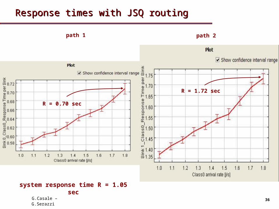
Response times with JSQ routingResponse times with JSQ routing

path 1 path 2

R = 1.72 sec

R = 0.70 sec




CASE STUDY 3CASE STUDY 3Resource Contention Resource Contention

(use of Finite Capacity Regions - FCR)(use of Finite Capacity Regions - FCR)

contention of componentscontention of componentshardware: I/O devices, memory, servers, ...hardware: I/O devices, memory, servers, ...

software: threads, locks, semaphores, ...software: threads, locks, semaphores, ...bandwidth bandwidth

open modelopen modelsingle class workloadsingle class workload

JSIMgraphJSIMgraph



modeling contention modeling contention

fixed number of hw/sw components (threads, db locks, semaphores, ...)

clients compete for the available component free request execution timerequest execution time: wait time for the next free component

+ wait time for the hardware resources (CPU, I/O, ...) + execution time

request interarrival times exponentially distributed payload of different sizes (exponentially distributed) evaluateevaluate the execution time of requests when the number of

clients ranges from 1 to 20 and the number of components ranges from 1 to 10 (∞), evaluate the drop rate and the wait time in queue for the next available component

implement several models with different level of completeness


threads (resource hw/sw) contention (simple model)threads (resource hw/sw) contention (simple model)

serverserver

...

...

sinksink

threads = 1÷∞threads = 1÷∞

clientsclients

thread requests queue(inside the server)

...

...

λλ=1=1÷20 r/s÷20 r/s

CPUCPU I/OI/O

DDCPUCPU=0.010s=0.010s

DDI/OI/O=0.047s=0.047s


model definition model definition (unlimited threads and queue size)(unlimited threads and queue size)

λ = 1 ÷ 20 req/sec

source of requests

queue resource

sink

name of the model

fraction of capacity used

selection of perf.indices

simulation results

fraction of n.o of requests


input parameters input parameters (service demands)(service demands)

mean service time = 0.010 s

mean service time = 0.047 s


system Response time system Response time ((λλ=20 req/sec)=20 req/sec)

confidence interval

transient duration

the number of samples analyzed is greater than the max defined here

perf.indexes selected

default valuesof parameters

actual sim. parameters

43

λλ=1÷20 req/s, =1÷20 req/s, unlimited threads & queue sizeunlimited threads & queue size (JSIMgraph)(JSIMgraph)

UI/O = λDI/O = 20*0.047 = 0.94 (exact)

Utilization of I/O

throughput

system Response time

same as λno limitations

R = 0.784 s (sim)0.931 (sim)

X = 19.86 r/s

system Power

R = 0.795 s (exact)



Number of requests Number of requests (unlimited threads & queue size)(unlimited threads & queue size)

0.25 req.15.39 req

N = 15.64 req (sim)

N = XR = 15.91 req (exact)


set of a Finite Capacity Region – FCRset of a Finite Capacity Region – FCR

step 1 – select the componentsof the FCR

step 2 – set the FCR

region with constrainednumber of customers

drop

queue


FCR parametersFCR parameters

global capacity of the FCR

max number of requests per class in the FCR

drop the requests when the regioncapacity is reached

(for both the constraints)


system Number of requests system Number of requests (limited n. threads and drop)(limited n. threads and drop)

5 threads

unlimited

10 threads

15 threads


Utilization of I/O server Utilization of I/O server (limited n. threads and drop)(limited n. threads and drop)

10 threads

unlimited 15 threads

5 threads


system Response time system Response time (limited n. threads and drop)(limited n. threads and drop)

5 threads10 threads

unlimited 15 threads


external finite queue for limited threads external finite queue for limited threads

serverserver..

...

.

sinksink

threads = 5threads = 5

clientsclients

queue for threads with finite capacity(outside the server)

λλ==20 r/s20 r/s

serverserver

DDserverserver=0.047s=0.047s

Blocking AfterService policy

queuequeue

drop policy

the queue for threads is limited (e.g., to limit the number of connections in case of denial of service attack, to guarantee a negotiated response time for the accepted requests, ...)

the requests arriving when the queue is full are rejected (drop policy) the number of threads is limited and the requests are queued in a resource

different from the server (load balancer, firewall, ...) evaluate the combination of different admission policies


set Block After Service (BAS) blocking policyset Block After Service (BAS) blocking policy

max number of requests in the station

station with finite capacity

selection of the BAS policy

BAS policy: requests are blocked in the sender station when the max

capacity of the receiveris reached


λ=20 req/s N R U X Drop Queue and Server stations

Qsize= ∞ QQ

Ser=5, queue SS0

16.110

0.770

0.9520.06 0

Qsize= ∞ QQSer=5, BAS SS

11.034.77

0.530.24

00.923

19.82 0

Qsize=5 drop QQSer=5, BAS SS

0.943.82

0.050.20

00.88

18.76 1.14

Qsize= ∞ QQSer=5, drop SS

02.34

00.136

00.812

17.16 2.866

ServerQueue

∞∞ 55∞∞

ServerQueue

∞∞ 55

BASBAS

ServerQueue

55 55

BASBAS

dropdrop

ServerQueue

∞ 55dropdrop

different admission policies for Queue and Serverdifferent admission policies for Queue and Server


CASE STUDY 4CASE STUDY 4

Multi-Tier Applications and Web ServicesMulti-Tier Applications and Web Services(Worker Threads, Workflows, (Worker Threads, Workflows,

Logging, Distributions)Logging, Distributions)

closed modelsclosed modelssingle class and multiclass workloadssingle class and multiclass workloads

fork-joinfork-join

JSIMgraph+JWATJSIMgraph+JWAT



performance evaluation of a multi-tier applicationperformance evaluation of a multi-tier application

multi-tier application serves a transactional workloadtransactional workload which requires processing by an application server (AS)application server (AS) and by a database (DB)database (DB)

the AS serves requests using a fixed set of worker threadsworker threads requests waiting for a worker thread are queued by the

admission controladmission control system

utilization measurementsutilization measurements available for the AS and for the DB– know both for AS and DB the average service time S– e.g., linear regression estimate

U=SX+Y, U = utilization, X = throughput, Y =noise

evaluateevaluate response time for increasing worker threads


transaction lifecycletransaction lifecycle

Worker thread admission time

Service time (1)

Queueing time

DB query time (1)

Service time (2)

Service time (3)

DB query time (2)

ServerResponsetime

Network latency (1)

Network latency (2)

Client-Side

Application Server

RequestResponsetime

Request arrives

Response arrives

Admission control

Load context in memory

Data access

Data access

CPU

CPU

CPU

DB Server

Worker Thread

Simultaneous Resource Possession


modelling abstraction (easier to define and study)modelling abstraction (easier to define and study)

Server admission time

Service time (1)

Queueing time

DB query time (1)

Service time (2)

Service time (...)

DB query time (2)

ServerResponsetime

Network latency (1)

Network latency (2)

Client-Side

Server-Side

RequestResponsetime

Request arrives

Response arrives

Admission control

Load context in memory

Data access

Data access

CPU

CPU+I/O

CPU+I/O

ApplicationServerSteps

DB ServerSteps

Worker Thread


modelling multi-tier applicationsmodelling multi-tier applications

Exponential Distributions

Scpu = 0.072s Sdb = 0.032s

Zload = 0.015s

FCR Admission Policy

FCR Capacity

FCR4 Servers (Cores)

FCR AdmissionQueue is Hidden !

PS scheduling

N=300 app users

send to jMVA

simulate


simulation vs jMVA modelsimulation vs jMVA model

FCR not included in product-form model


SAP Business Suite [Li, Casale, Ellahi; ICPE 2010]SAP Business Suite [Li, Casale, Ellahi; ICPE 2010]

MMVA M MS

S

SIMREAL

R

RR

S

Quad-Core ServerN=300 users

Response Time


what-if analysis – adding a web service classwhat-if analysis – adding a web service class

some requests now access the service composition engineservice composition engine of the multi-tier application to create a business travel plan

services are composed on the fly composed on the fly from external providers (travel agencies, flight booking service) according to a workflow

worker thread remains busy for the entire duration of the web service workflow

evaluateevaluate end-to-end response time for each class


business trip planning (BTP) web service business trip planning (BTP) web service

FCR Class-Based Admission

N=300 app usersNbtp=50 BTP users

pBTP=1.0

Sbtp =?, Exp?


BTP web service sub-modelBTP web service sub-model

Logger

S0=?, Exp?

Zsce=0.025s, Exp

N=1 WS instanceS1=?, Exp?

S2=?, Exp?


jWAT – Workload Analysis TooljWAT – Workload Analysis Tool

Specify Format

Column-Oriented Log File

Load Data

Data FormatTemplates


Ignore NegativeSamples

jWAT – data filteringjWAT – data filtering


jWAT – descriptive statisticsjWAT – descriptive statistics

Scatter plots

Histogram

c=std. dev. /mean

Hyper-Exp(c >1)


Outliers?

Scatter plot

jWAT – scatter plotjWAT – scatter plot


BTP web service sub-modelBTP web service sub-model

log inter-arrivaltimes

Zsce=0.025s, Exp

N=1 WS instance

S2=0.911HyperExp c=2.9081

S1=2.151, HyperExp c=1.689

S0=0.967 HyperExp c=3.1434


BTP response timesBTP response times

logarithmic transformation

e.g., Weibull,Lognormal.

Gamma


response time distribution – logger componentsresponse time distribution – logger components

Sbtp = 3.611s Gamma c=1.44

timestamp, class id, job id

timestamp, class id, job id

global.csvjob id (same throughout

simulation)

job classlogger id


response time distribution analysisresponse time distribution analysis

cumulative distribution

95th percentile

[seconds]

cdf

(matlab)

CONCLUSIONCONCLUSION


71


Final remarksFinal remarks

Analysis with Java Modelling Tools (http://jmt.sf.net) – Queueing network simulation

– Bottlenecks identification

– Workload analysis

– Mean value analysis

– ...

JMT-Based examples and exercises (http://perflib.net) Topics not covered by this tutorial

– jMCH

– Burstiness analysis

– Trace-driven simulation

– ...

JMT discussion forum: http://sourceforge.net/forum/?group_id=163838


ReferencesReferences

G.Casale, G.Serazzi. Quantitative System Evaluation with Java Modelling Tools (Tutorial).in Proc. of ACM/SPEC ICPE 2011 (companion paper).

M.Bertoli, G.Casale, G.Serazzi. User-Friendly Approach to Capacity Planning Studies with Java Modelling Tools, in Proc. of SIMUTOOLS 2009.

M.Bertoli, G.Casale, G.Serazzi. JMT - Performance Engineering Tools for System Modeling.ACM Perf. Eval. Rev., 36(4), 2009

M.Bertoli, G.Casale, G.Serazzi. The JMT Simulator for Performance Evaluation of Non Product-Form Queueing Networks, in Proc. of SCS Annual Simulation Symposium 2007, 3-10, Norfolk, VA, Mar 2007.

M.Bertoli, G.Casale, G.Serazzi. Java Modelling Tools: an Open Source Suite for Queueing Network Modelling and Workload Analysis, in Proc. of QEST 2006, 119-120, Sep 2006.

E.Lazowska, J.Zahorjan, G.S.Graham, K.C.Sevcik, Quantitative System Performance: Computer System Analysis Using Queueing Network Models, Prentice-Hall, 1994.

K.Pawlikowski: Steady-State Simulation of Queuing Processes: A Survey of Problems and Solutions. ACM Comput. Surv. 22(2): 123-170, 1990.

P.Heidelberger and P.D.Welch. A spectral method for confidence interval generation and run length control in simulations. Comm. ACM. 24, 233-245, 1981.

S.C.Spratt. Heuristics for the startup problem. M.S. Thesis, Department of Systems Engineering, University of Virginia, 1998.

Contact us!Contact us!

[email protected]@polimi.it


74

G.Casale – G.Serazzi 1 Quantitative System Evaluation with Java Modelling Tools Giuliano Casale...

Documents

Transcript of G.Casale – G.Serazzi 1 Quantitative System Evaluation with Java Modelling Tools Giuliano Casale...