![The GBAS Landing SystemThe GBAS Landing SystemTitle: Microsoft PowerPoint - Boeing GBAS Presentation, Beijing, October 29, 2009.ppt [兼容模式] Author: Shile Created Date: 11/10/2009](https://static.fdocuments.net/doc/165x107/5a727f467f8b9ac0538da536/the-gbas-landing-systemthe-gbas-landing-systemtitle-microsoft-powerpoint-boeing.jpg)
GBAS Ionospheric threat evaluation in the mid-latitude ...
50
GBAS Ionospheric threat evaluation in the mid-latitude Australian region Analysis, results and recommendations Workshop on Ionospheric Data Collection, Analysis and Sharing Dr Michael Terkildsen May 2011
Transcript of GBAS Ionospheric threat evaluation in the mid-latitude ...
GBAS Ionospheric threat evaluation in the mid-latitude Australian region Analysis, results and recommendations
Workshop on Ionospheric Data Collection, Analysis and Sharing
Dr Michael TerkildsenMay 2011
ssomsri
Text Box
IDCAS Workshop - SP/5

Outline• Ionospheric Prediction Service (IPS)• Recap: Challenges for GBAS posed by the
ionosphere• GBAS Iono threat model evaluation for Australia
– Scope of study– Results of analysis– Assumptions, limitations, recommendations
• Lessons learned from threat model evaluation• Ionospheric data sources• Future directions in ionospheric modelling

Ionospheric Prediction Service (IPS)• Formed in 1949• Originally concerned mostly with HF
communication• Now within Australian Bureau of Meteorology• Today, HF customer base still very important but
many other ‘space weather’ customers • Perform consultancies as well as providing
general space weather services and products• Australian Space Forecast Centre (ASFC) and
real time website: http://www.ips.gov.au• Daily S/W bulletin, web and email/SMS alerts

Ionospheric effects on GPS augmentation
http://www.nap.edu/catalog/12507.html
Solar Radio Bursts
(ionosphericdelay error
due to spatial gradients)

The solar cycle
w w w . i p s . g o v . a u
Priorities for the future?

Important latitude regimes for GPS effects
Low latitude/Equatorial region:Ionospheric scintillation, plasma bubbles, large TEC gradients, equatorial fountain, sub-equatorial anomalies. Driver of disturbances impacting mid- latitudes, particularly during storm-time.
Mid-latitude region:Mostly smaller gradients, strong diurnal pattern, lower spatial and temporal variability. Affected by strong storms, both from equatorial and high latitude regions.
High-latitudes/auroral/sub-auroral region: Strong gradients around auroral zone. Significant temporal variability on a range of time scales. Big storm response. Driver of disturbances propagating to mid- latitudes, particularly during storm-time.
Sub-equatorial anomalies/crests

The Australian Ionosphere
• Predominantly ‘benign’ mid-latitudes
• Under storm conditions, influenced by both equatorial and auroral physics
• Study restricted to latitude range -40° < lat < -20° reflecting both data availability and ionospheric physics

Anomalous Ionospheric gradients in CONUS

Decorrelation of ionospheric error
GBAS ground station
GNSS satellite
Ionosphere
Ionospheric gradient
Satellite ephemeris ERRORS
Clock ERRORS
Ionospheric ERROR (δ1)
Tropospheric ERROR
Satellite ephemeris ERRORS
Clock ERRORS
Ionospheric ERROR (δ2)
Tropospheric ERROR
Broadcast CORRECTION
(integrated ERROR)
=
=
range

Slant ionospheric gradientGNSS satellite
Ionosphere
Ionospheric gradientIonospheric ERROR (δ1)
Ionospheric ERROR (δ2)
Ground Range
GrndRangeradSlantIonoG 12
IPP1IPP2
(mm/km)
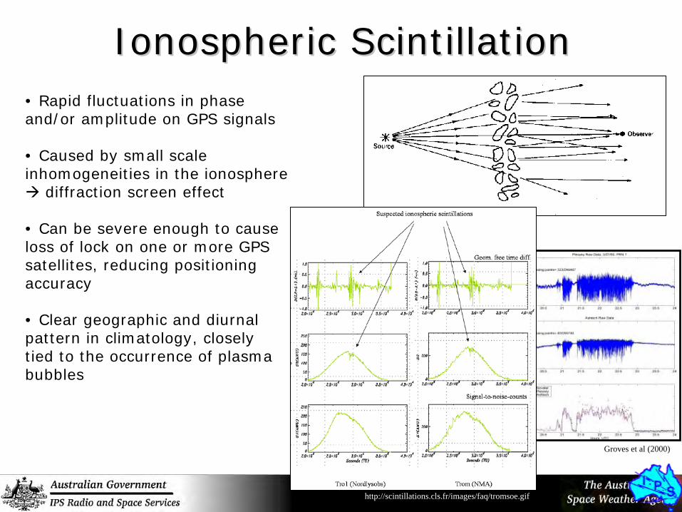
Ionospheric ScintillationIonospheric Scintillation• Rapid fluctuations in phase and/or amplitude on GPS signals
• Caused by small scale inhomogeneities in the ionosphere
diffraction screen effect
• Can be severe enough to cause loss of lock on one or more GPS satellites, reducing positioning accuracy
• Clear geographic and diurnal pattern in climatology, closely tied to the occurrence of plasma bubbles
http://scintillations.cls.fr/images/faq/tromsoe.gif
Groves et al (2000)
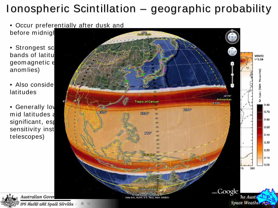
• Occur preferentially after dusk and before midnight (~18 -24 Local Time)
• Strongest scintillation occurs in two bands of latitude 5-15 degrees from the geomagnetic equator (sub-equatorial anomlies)
• Also considerable scintillation at high latitudes
• Generally low levels of scintillation at mid latitudes although can at times be significant, especially for high phase sensitivity instruments (eg radio telescopes)
Ionospheric Scintillation Ionospheric Scintillation –– geographic probabilitygeographic probability
w w w . i p s . g o v . a u

w w w . i p s . g o v . a u
Solar radio bursts
Dilution of Precision (DOP)
109876543
<2
GDOP
Sate
llite
Ele
vatio
n [
0 –
90 d
eg ]
Time (UT) [ 36 minute period ]
987654321
Satellite SNRLevelOccur during solar active conditions
Can have strong spectral peaks near the GPS L-band frequencies and thus act as a noise source to GPS receivers in the sunlit hemisphere
Result in reduced SNR for GNSS satellite tracking with potential for loss of lock on one or multiple satellites for affected receivers
Resultant GPS Dilution Of Precision (DOP)

GBAS iono threat model Simplified ionospheric threat model included in the (CONUS certified) Smartpath design for GBAS (Honewell ECM 10023, 2010)Specifies threat only in terms of ionospheric spatial gradients

2. Methodology• Storm identification - positive phase geomagnetic ‘superstorms’
• Data sourcing - dual frequency GPS RINEX data from all available short and long baseline regional CORS networks
• Network evaluation - capacity of networks to detect ionospheric gradients based on network geometry
• Data pre-processing - standard GNSS algorithms
• Identification of potential high gradient regions• Auto-processing for large gradient events• Manual vetting• Gradient analysis• Context of existing ionospheric threat modelFollo
ws
orig
inal
GB
AS
io
noth
reat
ana
lysi
s

Storm candidate identification• Major geomagnetic storms list (Kp > 8)• Restriction to positive phase storms in
Aus. longitude sector only (using onset time of storm and independent ionospheric observations)
• Reduced list of 8 storms since 2000

7. Ionospheric Storm AnalysisIonospheric storm threat :: Australian region
0
50
100
150
200
250
300
350
400
450
500
0 10 20 30 40 50 60 70 80 90
GPS satellite elevation angle [°]
Iono
sphe
re m
axim
um s
lant
gra
dien
t [m
m/k
m]
Figure 7-2. Anomalous ionospheric gradient parameters of ionospheric storms in the Australian region in context of the final (Smartpath) GBAS ionospheric threat model. The upper boundary of the threat model is indicated by the solid black line. All observations fall well within the bounds of the threat model
Smartpath
iono
threat model
Data for ionospheric characterisation
What data is required?From when?How much?Data specifics? (sampling rates, network
geometries)
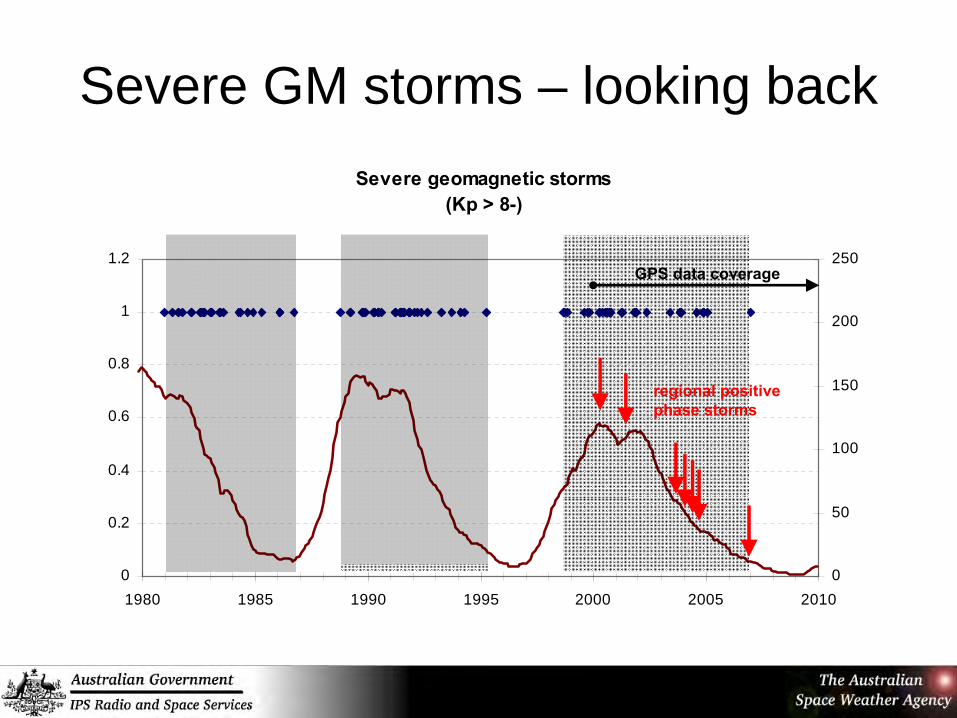
Severe GM storms – looking backSevere geomagnetic storms
(Kp > 8-)
0
0.2
0.4
0.6
0.8
1
1.2
1980 1985 1990 1995 2000 2005 20100
50
100
150
200
250GPS data coverage
regional positive phase storms

GNSS data sourcing:– Requirement for historical data covering the
largest ionospheric storms of the previous solar cycle
– Sufficient short baseline GNSS network geometry to enable detection of the full spectrum of ionospheric gradients
– High resolution (1-2s) data
Data for ionospheric characterisation

GNSS data sourcing:– Standard RINEX data format– Ionospheric scintillation (ISM or derived from
>1Hz GNSS and use of ROTI, DROTI, or comparable parameter)
Data for ionospheric characterisation

GNSS Data Sources• Australia dual frequency GPS (CORS) networks
- Geoscience Australia (ARGN, SPRGN)- Victorian Department of Sustainability and Environment
(GPSnet)- Queensland Department of Environment and Resource
Management (SunPOZ) - Landgate, Western Australia - National Measurement Institute, Sydney - IPS Radio & Space Services, Bureau of Meteorology- International GNSS Service (IGS)- Land Information New Zealand (PositioNZ)- [NSW CORSnet]

Network Geometry• GPS data limitations in Australia
greater emphasis on evaluating capacity of individual networks and network combinations to detect ionospheric gradients in present study
Analyse distribution of inter-station spacings and network geometry to confirm gradient detection capacity

GPS network map (old)
karr
darw / darr
tow2
jab2
alic
yar2 / yar3 / yarr
hil1
cedu
mobs
hob2
bur1
sunm
ade1
pert / nnor
ARGN GPS Network
State CORS Networks
str1 / str2 sydn / nmi1
tidb / tid1 / tid2
park
South-East INSET

GPS network map (SE detail)ARGN GPS Network
State CORS Networks
mobs
sunm
ade1str1 str2 sydn
nmi1
tidbtid1tid2
250km (approx)
park
GPSNet
INSET
SydNET
INSET
SunPOZ
INSET
South-East
SANSW
Vic
Qld

Example of ionospheric coverage

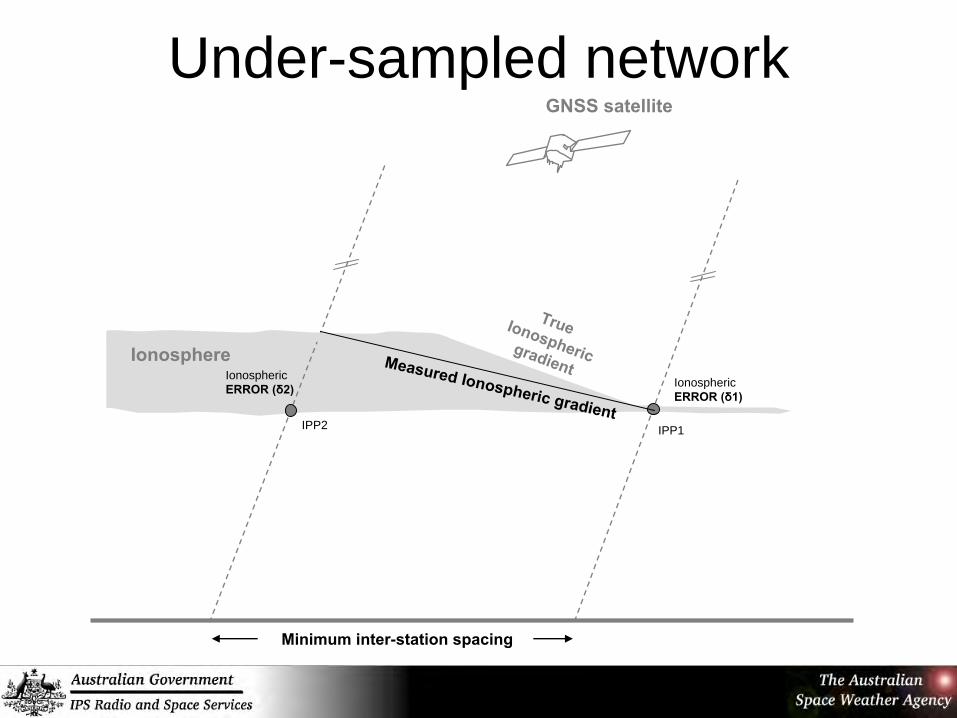
Under-sampled networkGNSS satellite
Ionosphere
True Ionospheric gradientIonospheric ERROR (δ1)
Ionospheric ERROR (δ2)
Minimum inter-station spacing
IPP1IPP2
Measured Ionospheric gradient

Maximum inter-station spacing
Closely-spaced networkGNSS satellite
Ionosphere True Ionospheric gradientIonospheric ERROR (δ1)
Ionospheric ERROR (δ2)
IPP1IPP2
Note: As separation 0,
gradient observations
dominated by Rx bias and
measurement noise

Threshold inter-station spacing for gradient detection
Threshold station separation for iono gradient detection
10
100
1000
10000
0 50 100 150 200 250 300 350 400
Iono gradient (mm/km)
Threshold station separation
(km)
Max Iono Delay
30m (185 TECU)25m (154 TECU)
20m (123 TECU)
15m (92.6 TECU)
10m (61.7 TECU)
5m (30.9 TECU)
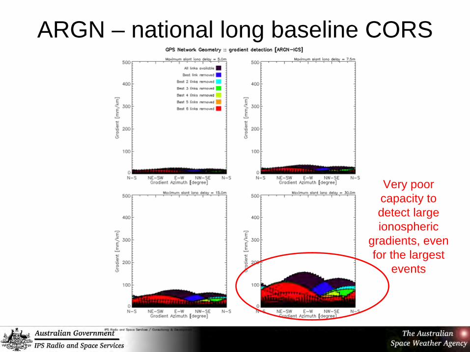
ARGN – national long baseline CORS
Very poor capacity to detect large ionospheric
gradients, even for the largest
events

SunPOZ
-
State CORS Queensland
clevsunm
land
ARGN GPSSunPOZ CORS
ipsw
25 km
been
bund
NSW
Qld
SunPOZ
Some assumptions1) Longitudinal invariance in storm response2) Anomalous gradient occurrence
exclusively during superstorms3) Study period 2000-2008 representative4) Restricted region of applicability

A1. Longitudinal ‘invariance’ of ionospheric response
• Ionosphere described more strongly by latitude than longitude.
• Although there are longitude sectors with unique characteristics (eg CONUS) these are very broad local time sectors
• IPS experience does not suggest any major difference in ionospheric characteristics between the East and West coasts of Australia

A2. Validation of storm selection
• Additional work at IPS on validating this assumption
• Ionospheric gradient index derived for this validation, and used to automatically process/analyse four years of short- baseline GPS data to confirm association of anomalous gradients with superstorms
The largest anomalous ionospheric gradients in the Australian mid-latitude region occur during geomagnetic “superstorms” (as identified by threshold level of Kp), more specifically those storms that have a positive phase in the Australian longitude sector.

Anomalous gradient event detection using gradient index
Ionospheric slant gradient detectionSunPOZ 2004
0
5
10
15
20
25
30
35
40
45
50
300 305 310 315 320 325 330 335 340
Day of year (2004)
Ave
rage
d sl
ant g
radi
ent [
mm
/km
]

Max Ionospheric gradient index during storms (2002-2005)

A3. Representative study period
• Qualified. Representative of regional anomalous ionospheric gradients over last solar cycle
• Likely representative of anomalous ionospheric gradients in the Australian region
• Recommend ongoing monitoring of anomalous ionospheric conditions for further confidence (eg CONUS experience)
This study covering the period 2001 – 2008 is representative of the full range of ionospheric gradients that may occur in the Australian region.

A4. Region of applicability• Results limited to Australian longitude sector, mid-
latitudes (-40° < glat < -20°)• Southern boundary: Dictated by archive data coverage
(poor short-baseline coverage in Tas)• Northern boundary: Dictated by archive data
coverage, as well as the unique ionospheric physics of the equatorial zone.
• Studies of the impact of the equatorial ionosphere on GBAS-like systems is ongoing in other states
• Recommend advance iono monitoring for northern Australia for future certification of GBAS

Extra slides• Extra slides follow

Real-time regional TEC model• IPS has developed a Kalman
Filter driven real-time TEC modelling capability
• The model uses Spherical Cap Harmonic Analysis (SCHA) for spatial mapping of TEC
• The filter states are the SCH basis co-efficients, the GPS Rx biases and a plasmaspheric TEC scaling factor.
• Utilises data from > 60 GPS sites across the region, along with ~8-10 ionosondes, with capacity to expand further
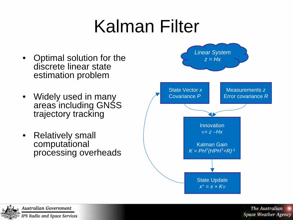
Kalman Filter• Optimal solution for the
discrete linear state estimation problem
• Widely used in many areas including GNSS trajectory tracking
• Relatively small computational processing overheads
Linear Systemz = Hx
State Vector xCovariance P
Measurements zError covariance R
Innovation= z –Hx
Kalman Gain K = PHT(HPHT+R)-1
State Updatex+ = x + K

3D Model Development• A full 3D ionosphere + plasmasphere real time model is
currently under development.
• Model driven by a range of input data, including:– ground based GPS– Ionosonde vertical soundings– Ionosonde oblique soundings– LEO satellite GPS– LEO satellite radio occultation (RO) observations
• The current approach uses the NeQuick2 ionospheric profiler as a base vertical model, with free model parameters constrained by the real time input data and mapped in 2D using SCHA.


?
So what about the next solar activity cycle?
w w w . i p s . g o v . a u

w w w . i p s . g o v . a u
Priorities for the future?
w w w . i p s . g o v . a u
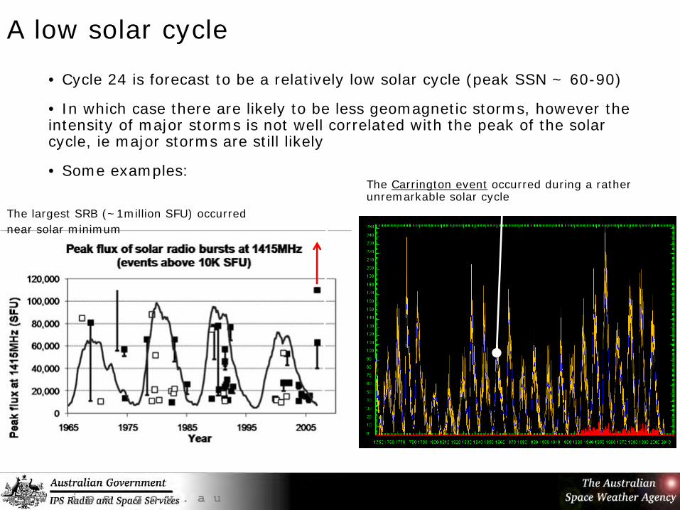
A low solar cycle
• Cycle 24 is forecast to be a relatively low solar cycle (peak SSN ~ 60-90)
• In which case there are likely to be less geomagnetic storms, however the intensity of major storms is not well correlated with the peak of the solar cycle, ie major storms are still likely
• Some examples: The Carrington event occurred during a rather unremarkable solar cycle
The largest SRB (~1million SFU) occurred near solar minimum


Space Weather
Solar Flare/ DSF
Coronal MassEjection (CME)
1-3 days propagationthrough solar wind
Solar ActiveRegion
Reaches ACE satellite~ 1 hour upstream(1-hour warning)
Shock hitsgeomagnetic field
(observed on ground)
Geomagneticstorm develops
(observed real time)
Ionosphericstorm develops
(observed real time)

IPS Extreme SpWx Event Alert Service• Under development at IPS• Very high alert threshold (minimise false positives)• Driven by growing demand for advance warning of
extreme space weather events from various critical industries (eg power networks, pipelines, SES)
• Implemented as a chain of alerts Sun-Earth during S/W event development, each building on the previous, with increasing probability estimates
• To provide sufficient lead time for industries to build awareness, prepare, and ultimately take action to minimise impact of extreme space weather events
• Output can be tailored to GBAS/aviation requirements such as ionospheric storm-front and gradient monitoring