Gauss-Seidel - contents.kocw.netcontents.kocw.net/KOCW/document/2016/chonnam/choiyonghoon/9.pdf ·...
25
Transcript of Gauss-Seidel - contents.kocw.netcontents.kocw.net/KOCW/document/2016/chonnam/choiyonghoon/9.pdf ·...

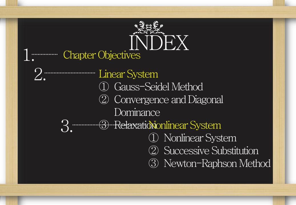
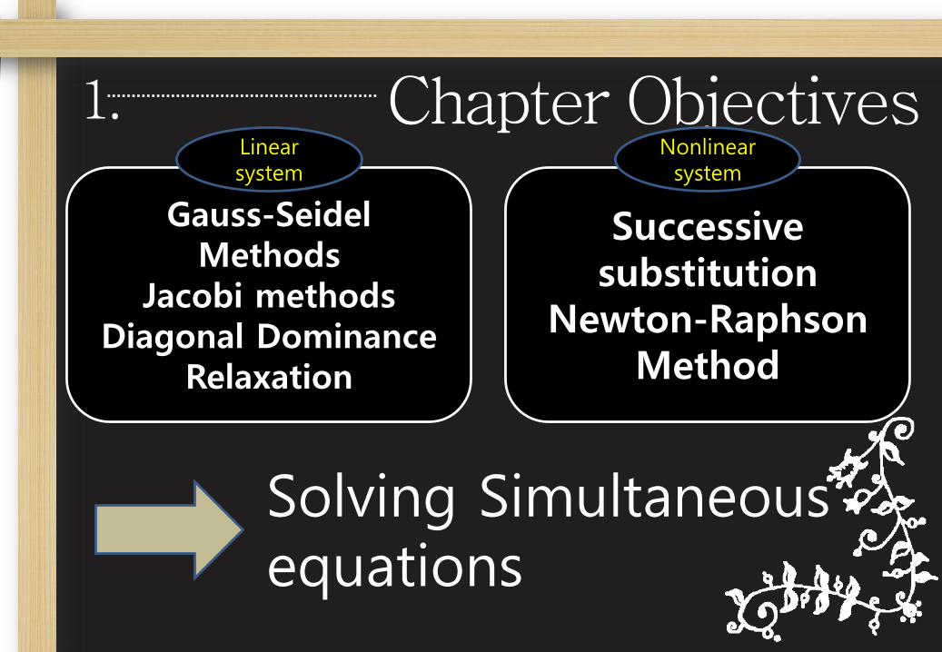
Gauss-Seidel Methods
Jacobi methodsDiagonal Dominance
Relaxation
Linear system
Successive substitution
Newton-RaphsonMethod
Nonlinear system
Solving Simultaneous equations
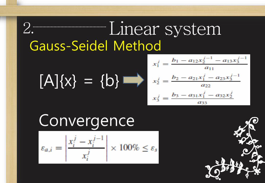
[A]{x} = {b}
Gauss-Seidel Method
Convergence
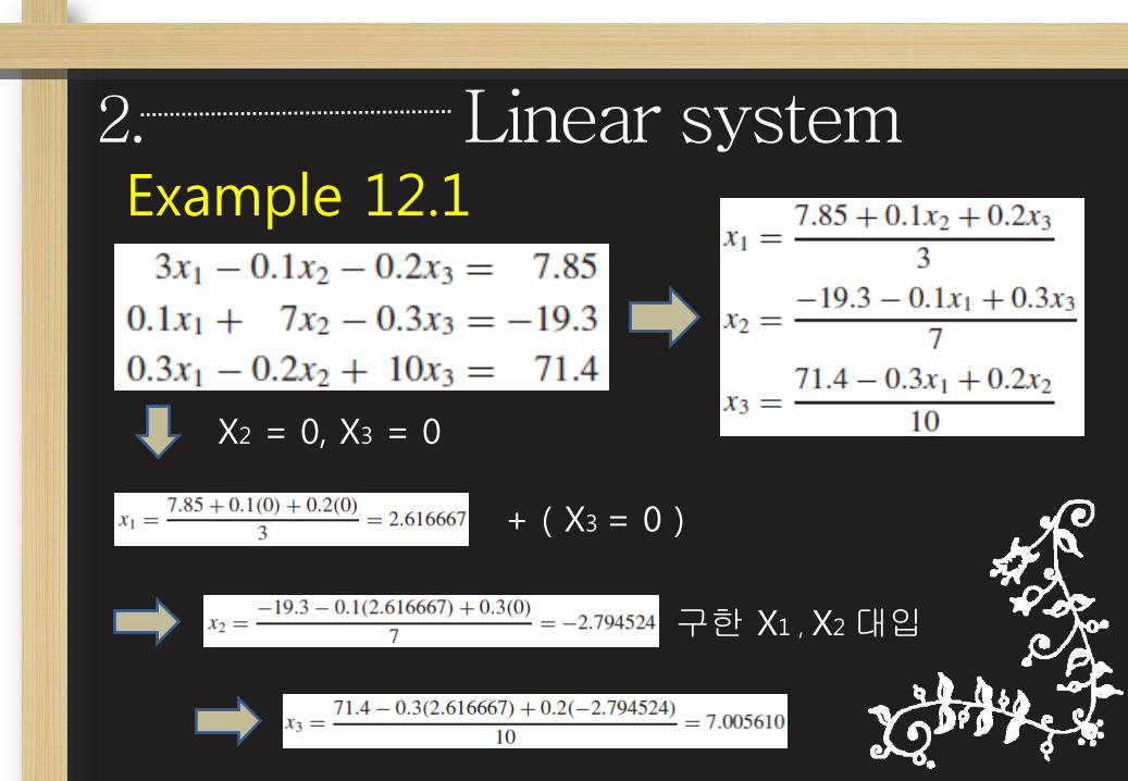
Example 12.1
X2 = 0, X3 = 0
+ ( X3 = 0 )
구한 X1 , X2 대입
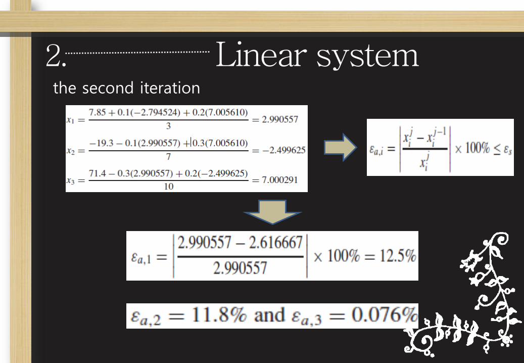
the second iteration
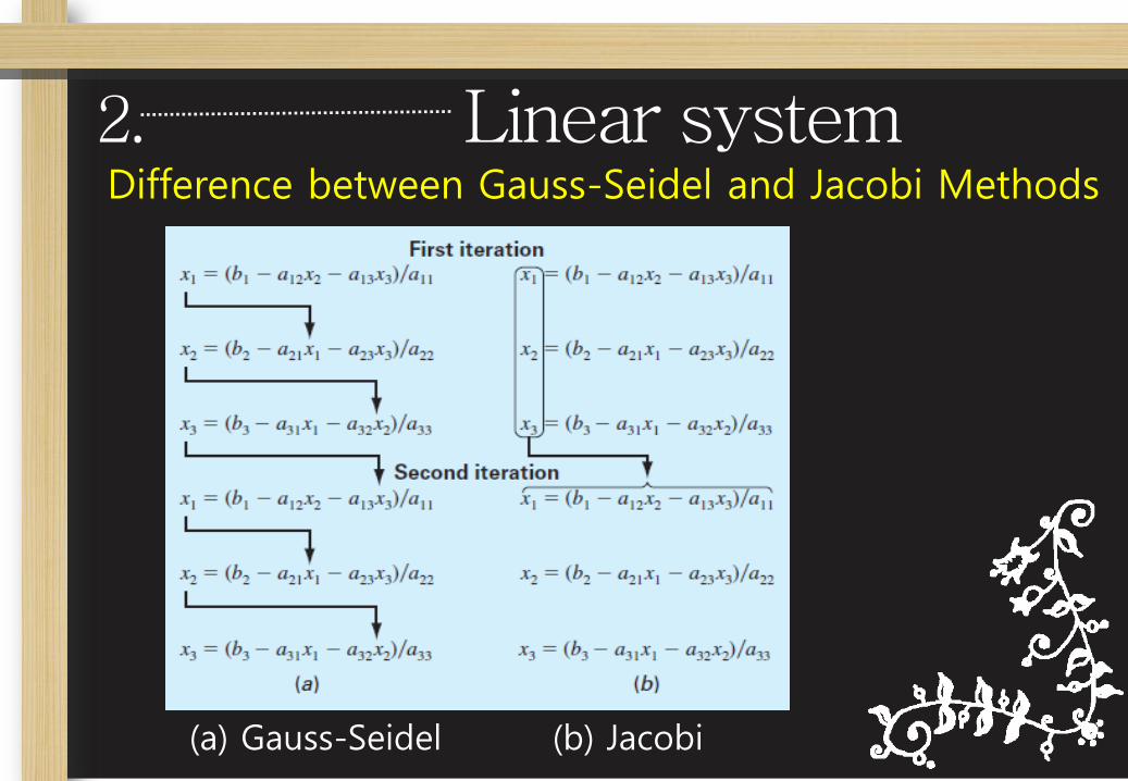
Difference between Gauss-Seidel and Jacobi Methods
(a) Gauss-Seidel (b) Jacobi
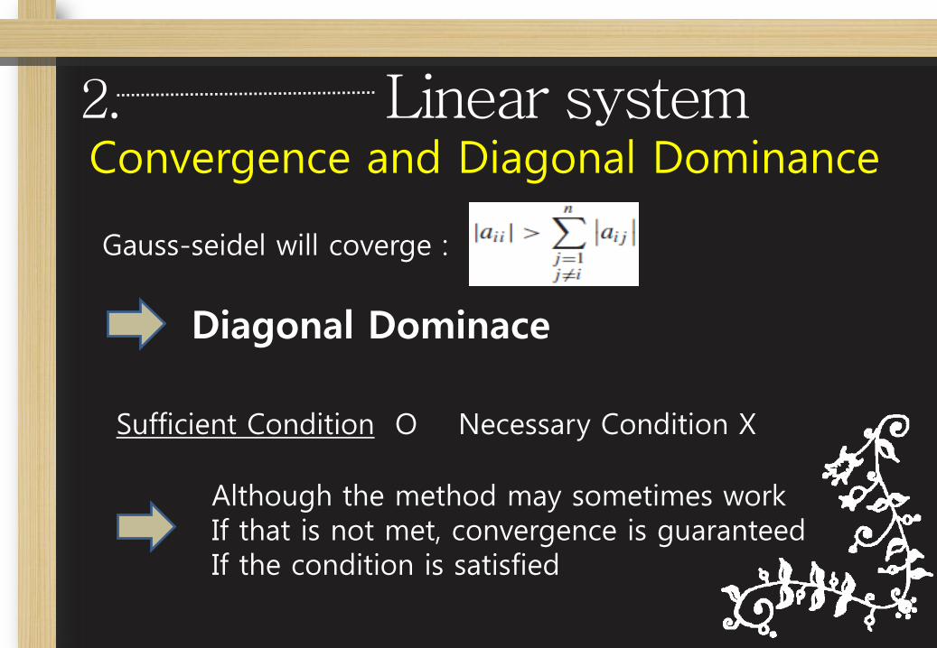
Convergence and Diagonal Dominance
Gauss-seidel will coverge :
Diagonal Dominace
Sufficient Condition O Necessary Condition X
Although the method may sometimes workIf that is not met, convergence is guaranteedIf the condition is satisfied
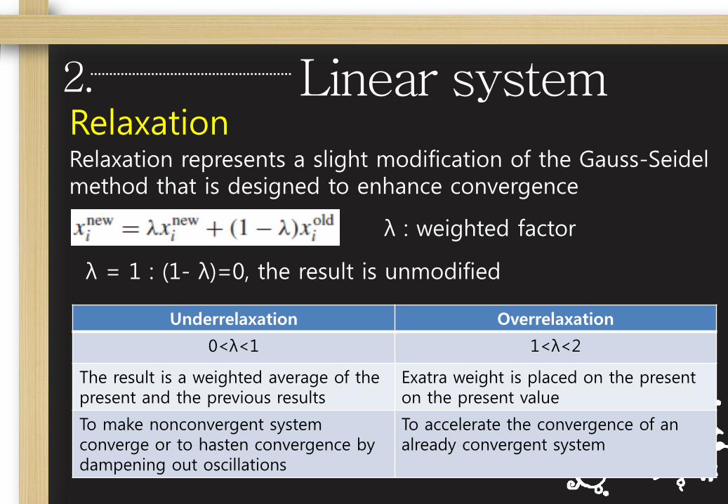
RelaxationRelaxation represents a slight modification of the Gauss-Seidel method that is designed to enhance convergence
λ : weighted factor
λ = 1 : (1- λ)=0, the result is unmodified
Underrelaxation Overrelaxation
0<λ<1 1<λ<2
The result is a weighted average of the present and the previous results
Exatra weight is placed on the present on the present value
To make nonconvergent system converge or to hasten convergence by dampening out oscillations
To accelerate the convergence of an already convergent system
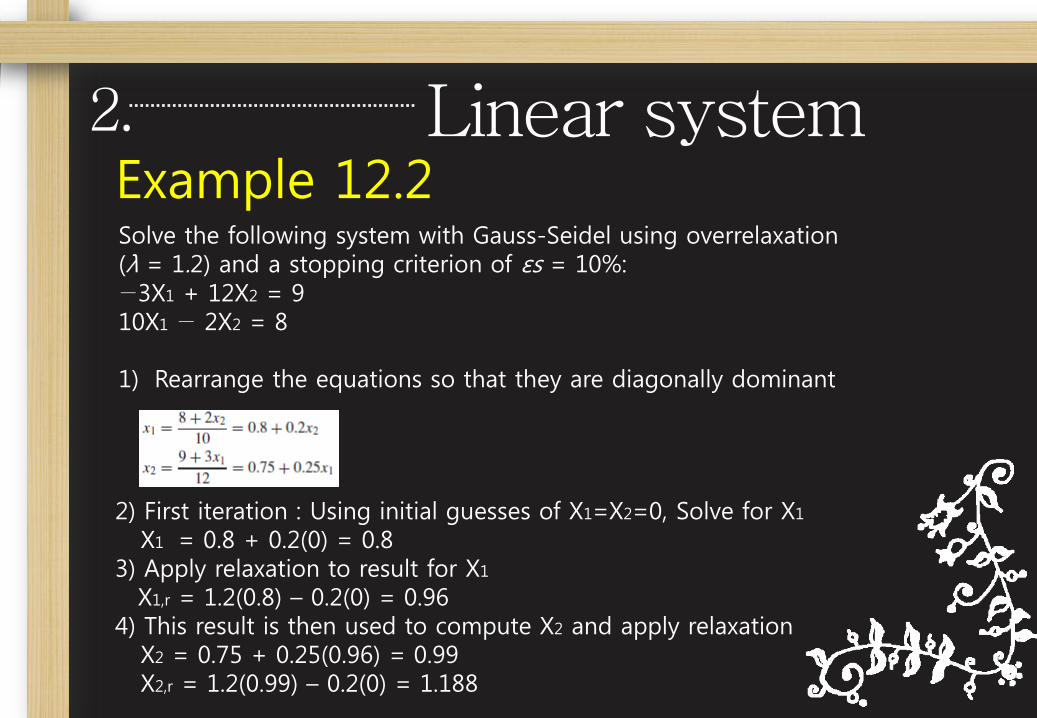
Example 12.2Solve the following system with Gauss-Seidel using overrelaxation(λ = 1.2) and a stopping criterion of εs = 10%:−3X1 + 12X2 = 910X1 − 2X2 = 8
1) Rearrange the equations so that they are diagonally dominant
2) First iteration : Using initial guesses of X1=X2=0, Solve for X1
X1 = 0.8 + 0.2(0) = 0.83) Apply relaxation to result for X1
X1,r = 1.2(0.8) – 0.2(0) = 0.964) This result is then used to compute X2 and apply relaxation
X2 = 0.75 + 0.25(0.96) = 0.99X2,r = 1.2(0.99) – 0.2(0) = 1.188
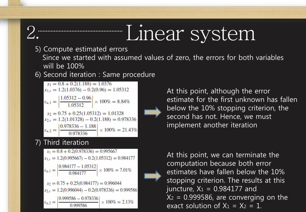
5) Compute estimated errors Since we started with assumed values of zero, the errors for both variables
d. will be 100%6) Second iteration : Same procedure
7) Third iteration
At this point, although the error estimate for the first unknown has fallen below the 10% stopping criterion, the second has not. Hence, we must implement another iteration
At this point, we can terminate the computation because both error estimates have fallen below the 10% stopping criterion. The results at this juncture, X1 = 0.984177 andX2 = 0.999586, are converging on the exact solution of X1 = X2 = 1.
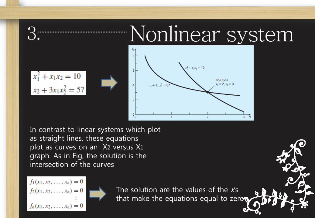
In contrast to linear systems which plot as straight lines, these equationsplot as curves on an X2 versus X1
graph. As in Fig, the solution is the intersection of the curves
The solution are the values of the x’s that make the equations equal to zero
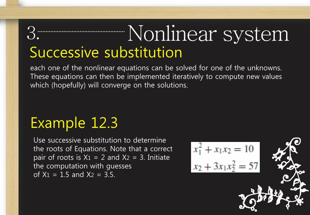
Successive substitutioneach one of the nonlinear equations can be solved for one of the unknowns. These equations can then be implemented iteratively to compute new values which (hopefully) will converge on the solutions.
Example 12.3Use successive substitution to determine the roots of Equations. Note that a correct pair of roots is X1 = 2 and X2 = 3. Initiate the computation with guessesof X1 = 1.5 and X2 = 3.5.
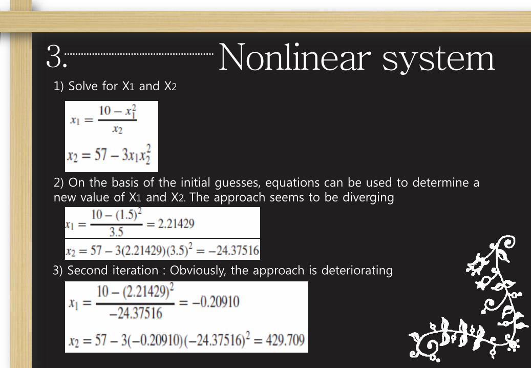
1) Solve for X1 and X2
2) On the basis of the initial guesses, equations can be used to determine a new value of X1 and X2. The approach seems to be diverging
3) Second iteration : Obviously, the approach is deteriorating
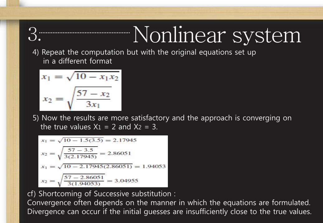
4) Repeat the computation but with the original equations set up in a different format
5) Now the results are more satisfactory and the approach is converging on the true values X1 = 2 and X2 = 3.
cf) Shortcoming of Successive substitution :Convergence often depends on the manner in which the equations are formulated.Divergence can occur if the initial guesses are insufficiently close to the true values.
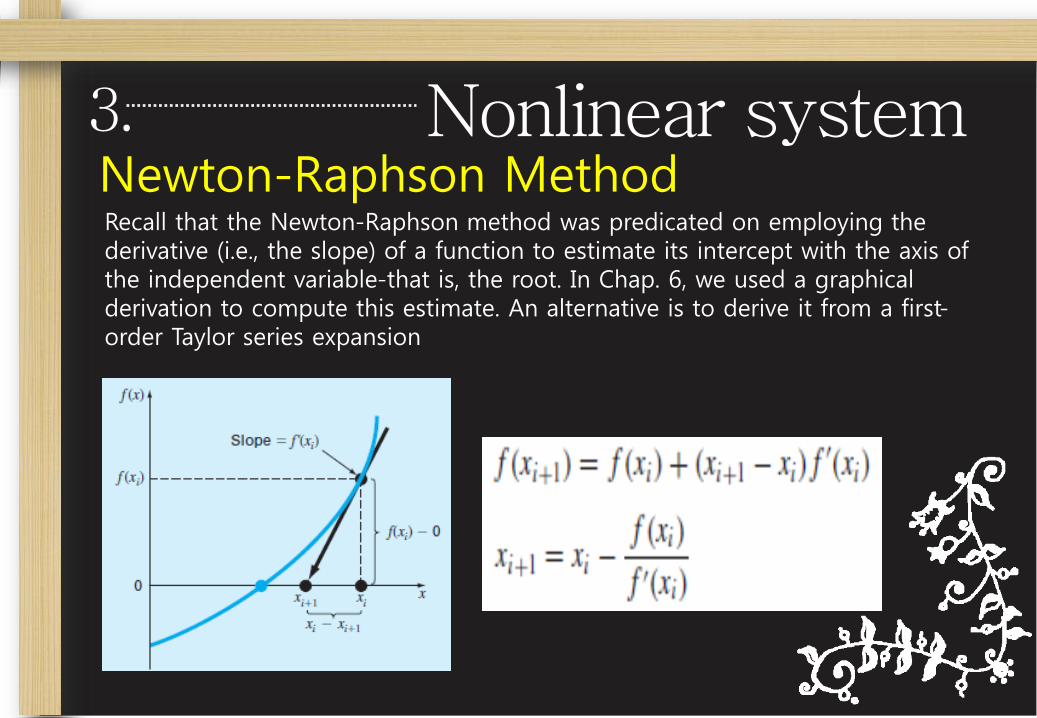
Newton-Raphson MethodRecall that the Newton-Raphson method was predicated on employing the derivative (i.e., the slope) of a function to estimate its intercept with the axis of the independent variable-that is, the root. In Chap. 6, we used a graphical derivation to compute this estimate. An alternative is to derive it from a first-order Taylor series expansion
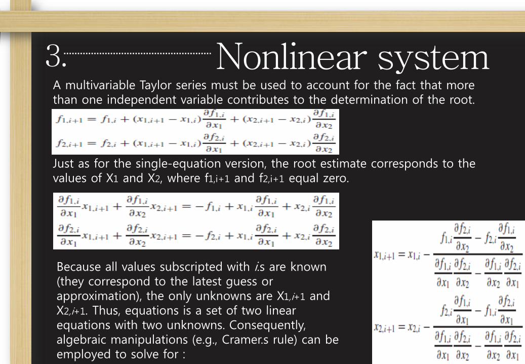
A multivariable Taylor series must be used to account for the fact that more than one independent variable contributes to the determination of the root.
Just as for the single-equation version, the root estimate corresponds to the values of X1 and X2, where f1,i+1 and f2,i+1 equal zero.
Because all values subscripted with i.s are known (they correspond to the latest guess orapproximation), the only unknowns are X1,i+1 and X2,i+1. Thus, equations is a set of two linear equations with two unknowns. Consequently, algebraic manipulations (e.g., Cramer.s rule) can be employed to solve for :
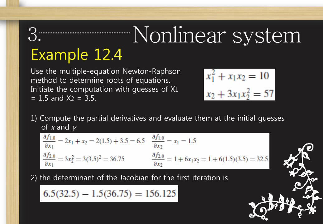
Example 12.4Use the multiple-equation Newton-Raphson method to determine roots of equations. Initiate the computation with guesses of X1
= 1.5 and X2 = 3.5.
1) Compute the partial derivatives and evaluate them at the initial guesses of x and y
2) the determinant of the Jacobian for the first iteration is
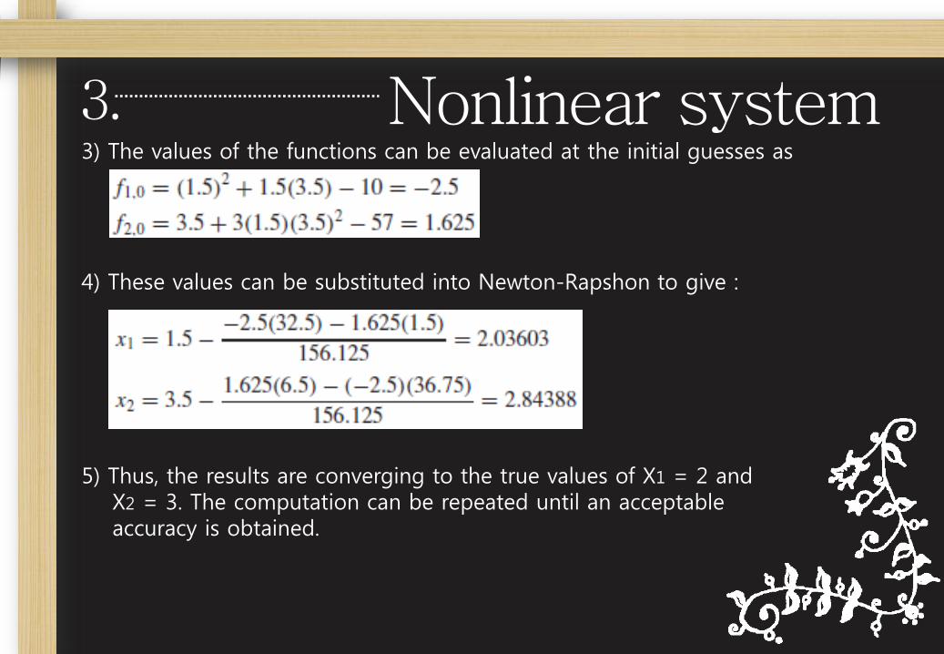
3) The values of the functions can be evaluated at the initial guesses as
4) These values can be substituted into Newton-Rapshon to give :
5) Thus, the results are converging to the true values of X1 = 2 and X2 = 3. The computation can be repeated until an acceptable accuracy is obtained.
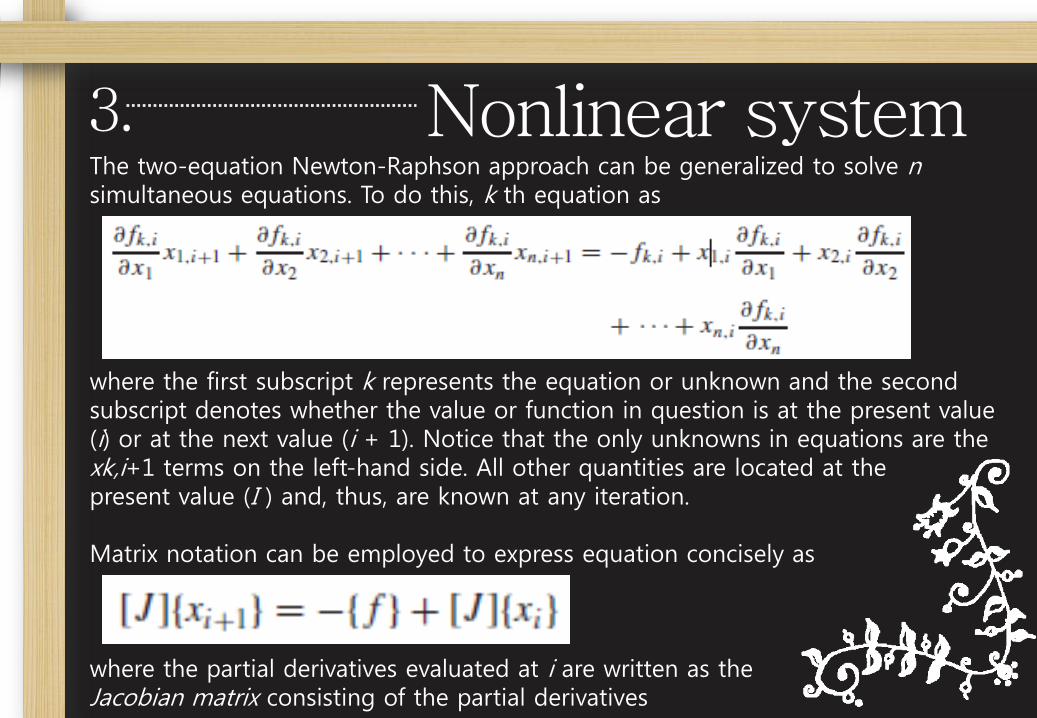
The two-equation Newton-Raphson approach can be generalized to solve n simultaneous equations. To do this, k th equation as
where the first subscript k represents the equation or unknown and the second subscript denotes whether the value or function in question is at the present value (i) or at the next value (i + 1). Notice that the only unknowns in equations are the xk,i+1 terms on the left-hand side. All other quantities are located at the present value (I ) and, thus, are known at any iteration.
Matrix notation can be employed to express equation concisely as
where the partial derivatives evaluated at i are written as the Jacobian matrix consisting of the partial derivatives
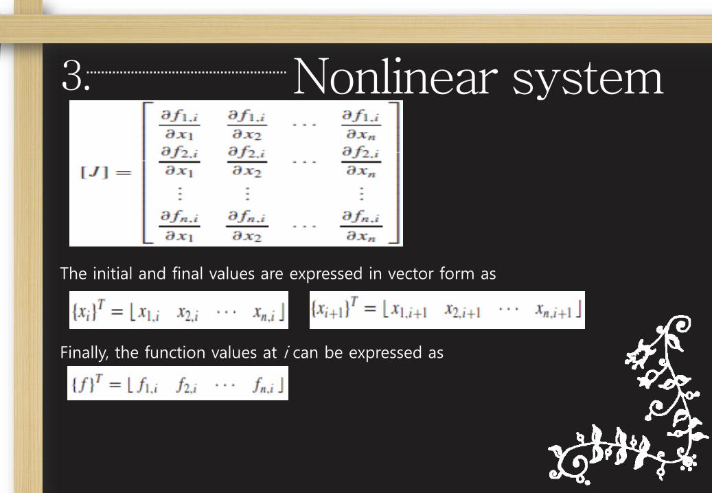
The initial and final values are expressed in vector form as
Finally, the function values at i can be expressed as
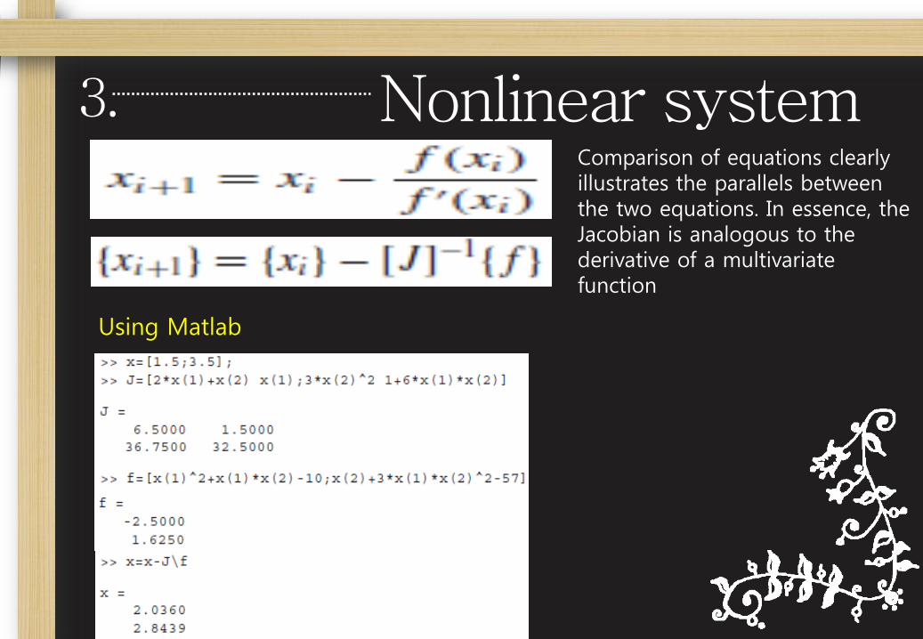
Comparison of equations clearly illustrates the parallels between the two equations. In essence, the Jacobian is analogous to the derivative of a multivariate function
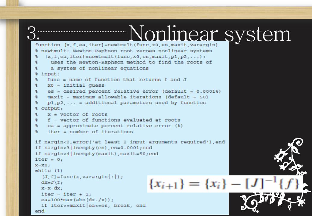
Using Matlab
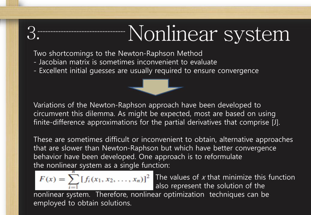
Two shortcomings to the Newton-Raphson Method- Jacobian matrix is sometimes inconvenient to evaluate- Excellent initial guesses are usually required to ensure convergence
Variations of the Newton-Raphson approach have been developed to circumvent this dilemma. As might be expected, most are based on using finite-difference approximations for the partial derivatives that comprise [J].
These are sometimes difficult or inconvenient to obtain, alternative approaches that are slower than Newton-Raphson but which have better convergence behavior have been developed. One approach is to reformulate the nonlinear system as a single function:
The values of x that minimize this function also represent the solution of the
nonlinear system. Therefore, nonlinear optimization techniques can be employed to obtain solutions.
![NM2012S-Lecture12-Iterative Methods.ppt [相容模式]berlin.csie.ntnu.edu.tw/Courses/Numerical Methods/Lectures2012S... · Gauss-Seidel Method • The Gauss-Seidel methodis the most](https://static.fdocuments.net/doc/165x107/5b18a0f07f8b9a28258bea5f/nm2012s-lecture12-iterative-berlincsientnuedutwcoursesnumerical.jpg)

![Flujo de Potencia [Modo de compatibilidad] - u-cursos.cl · Método de Gauss Método de Gauss ----SeidelSeidel La “Receta” para Gauss La “Receta” para Gauss ––Seidel Seidel](https://static.fdocuments.net/doc/165x107/5d3f527d88c993860c8d17eb/flujo-de-potencia-modo-de-compatibilidad-u-metodo-de-gauss-metodo-de.jpg)