Gasoline Prices, Government Support, and the Demand for

Hybrid Vehicles in the U.S.∗

Arie Beresteanu and Shanjun Li †

First Version: August, 2007

This Version: January, 2008

Abstract

Exploiting a rich data set of new vehicle registrations in 22 U.S. Metropolitan

Statistical Areas from 1999 to 2006, we analyze the determinants in the demand

for hybrid vehicles and examine government programs that aim to promote the

adoption of hybrid vehicles. We find that both the recent run-up in gasoline prices

from 1999 and federal income tax incentives are important in the diffusion of hybrid

vehicles, explaining about 14% and 27% hybrid vehicle sales in 2006, respectively.

We compare the current income tax credit program with a rebate program and find

that the rebate program needs less government revenue to achieve the same level of

average fuel-efficiency of new vehicles. The cost advantage of such a rebate program

is bigger with larger incentives.

∗We thank Paul Ellickson, Han Hong, Wei Tan, and Chris Timmins for their helpful comments.Financial support from Micro-Incentives Research Center at Duke University is gratefully acknowledged.

†Arie Beresteanu, Assistant Professor, Department of Economics, Duke University, Durham, NC27708-0097, arie@econ.duke.edu; Shanjun Li, Asssitant Professor, Department of Economics, SUNY-StonyBrook, Stony Brook, NY 11794-4384, shlli@notes.cc.sunysb.edu.

1 Introduction

Since their introduction into the U.S. market in 2000, hybrid vehicles have been in in-

creasingly strong demand: sales grew from less than 10,000 cars in 2000 to more than

250,000 in 2006. A hybrid vehicle combines the benefits of gasoline engines and electric

motors and delivers better fuel economy than its non-hybrid equivalent. Therefore, the

hybrid technology has been considered as a promising tool in the U.S. to reduce CO2

emission and air pollution and to achieve energy security. Following the recommendation

of the National Energy Policy Report (2001),1 the U.S. government has been supporting

consumer purchase of hybrid vehicles in the forms of federal income tax deductions before

2006 and federal income tax credits since then.

An active governmental role to support the diffusion of this technology can be justified

on the ground of environmental externalities and national energy interest: the adoption

of hybrid vehicles by U.S. drivers could be too low compared with the socially optimal

level because the individual benefit of driving a hybrid vehicle (relative to a conventional

vehicle) is smaller than the social benefit. The discrepancy between the individual benefit

and the social benefit can be further magnified by the high initial production cost of hybrid

vehicles due to the presence of significant economies of scale inherent in the automobile

manufacturing industry and by information spillovers among consumers and among firms

often present in the diffusion process of new technologies.2

The United States is increasingly dependent on foreign oil: the proportion of imports

in total petroleum products has reached 60 percent in recent years, largely driven by

growing motor gasoline consumption. Moreover, while producing an estimated 60 to 70

percent of total urban air pollution and 25 percent of total emission of smog-forming

1The report was written by the National Energy Policy Development (NEPD) Group established in2001 by George W. Bush. The goal of the group is to develop a national energy policy designed to promotedependable, affordable, and environmentally sound production and distribution of energy for the future.

2Stoneman and Diederen (1994) argues for more government attention to technology diffusion citingthe presence of imperfect information and externalities. Jaffe and Stavins (1999) focus on the gradualdiffusion of energy-conservative technologies and suggest the use of both economic incentives and directregulations.

1

pollutants, motor vehicles account for about 20 percent of the annual U.S. emissions of

carbon dioxide, the predominant greenhouse gas that contributes to global warming. To

address energy security and environmental problems, different policies have been proposed

such as increasing the federal gasoline tax, tightening Corporate Average Fuel Economy

(CAFE) Standards, and promoting the development and adoption of fuel-efficient tech-

nologies including the hybrid technology and the fuel cell technology. Many studies have

examined the first two alternatives, with the majority of them finding that increasing the

gasoline tax is more cost-effective than tightening CAFE standards.3 However, there exist

few studies that look at the adoption of hybrid technology and none of them examines the

effect of government support on solving energy dependence and environmental problems

through the diffusion of hybrid vehicles.

In this paper, we analyze the determinants of hybrid vehicle purchase, paying particular

attention to recent rising gasoline prices and government support. We investigate how

effective government support has been in promoting hybrid vehicle adoptions and to what

extent the hybrid technology can help the United States reduce gasoline consumption and

CO2 emissions. In addition, we examine the cost-effectiveness of the current income tax

credit program by comparing it with a rebate program. As outlined in the Energy Policy

Act of 2005, income tax credits exist to encourage the adoption of qualified energy-efficient

home improvement appliances, fuel-efficient vehicles, solar energy system, and fuel cell and

microturbine power systems. In the case of hybrid vehicles, the income tax credit reduces

the regular federal income tax liability of the hybrid vehicle buyer, but not below zero.4

Therefore, households whose income tax liability is smaller than the tax credit are not able

to enjoy the maximum possible incentive. Nevertheless, these households tend to have low

income and be more responsive to the incentives than high-income households. A rebate

program that offers equal subsidy to all the buyers of the same hybrid model, therefore,

3See for example, National Research Council (2002); Congressional Budget Office (2003); Austin andDinan (2005); Bento, Goulder, Henry, Jacobsen, and von Haefen (2005) ; and West and Williams (2005).

4The tax credit cannot be carried over to the future. Moreover, the credit will not reduce alternativeminimum tax (AMT) when it applies to a hybrid vehicle buyer.

2

may result in more hybrid sales than the tax credit program with the same amount of

total government subsidy. The better cost-effectiveness of a rebate program should also

hold in the income tax credit program for other energy-efficient products aforementioned.

Taking advantage of a rich data set of new vehicle registrations in 22 Metropolitan

Statistical Areas (MSA) from 1999 to 2006, we estimate a market equilibrium model with

both a demand side and a supply side in the spirit of Berry, Levinsohn, and Pakes (1995)

(henceforth BLP). The demand side is derived from a random coefficient utility model

and the supply side assumes that multiproduct firms engage in price competition. Similar

to Petrin (2002) and Berry, Levinsohn, and Pakes (2004), our estimation employs both

aggregate market-level sales data and household-level data. We use the 2001 National

Household Travel Survey (2001 NHTS) to augment aggregate sales data. Different from

these studies, we observe the sales of the same model in 22 markets and use product fixed

effects to control for price endogeneity due to unobserved product attributes. Therefore,

our estimation method does not rely on the maintained exogeneity assumption of observed

product attributes to unobserved product attributes, which is used to form moment con-

ditions in the literature.

Based on the structural parameter estimates, we first conduct counterfactual simula-

tions to evaluate the effect of rising gasoline prices and government support on the demand

for hybrid vehicles in the 22 MSAs. We find that both factors are significant in explaining

the increasing popularity of hybrid vehicles. However, due to the small market share of

hybrid vehicles, the reduction in both gasoline consumption and CO2 emission resulted

from government support on hybrid vehicle purchases has been inconsequential. With

the increasing number of hybrid models introduced into the market and increasing mar-

ket share of hybrid vehicles, government support should be able to make more significant

contribution toward achieving oil independence and environmental objectives. We then

compare the federal income tax credit program in 2006 with a rebate program in terms of

their cost-effectiveness. We find that the rebate programs costs less government revenue to

achieve the same average fuel-efficiency of new vehicle fleet in 2006, suggesting that rebate

3

programs should be favored over income tax credit programs to promote the adoption of

energy-efficient products.

Three recent papers have examined several issues related to hybrid vehicles. Kahn

(2008) studies the effect of environmental preference on the demand for green products

and finds a positive correlation between the adoption of hybrid vehicles and the percentage

of registered green party voters in California. Sallee (2008) studies incidence of tax credits

for Toyota Prius and shows that consumers capture the significant majority of the benefit

from tax subsidies. A more closely related study to ours, Gallagher and Muehlegger (2007)

estimate the effect of state and local incentives, rising gasoline prices, and environmental

ideology on hybrid vehicle sales and find all three very important. A major difference

between our study and these papers is that all of them focus on a single hybrid model or

hybrid vehicles alone while we take a structural method to estimate an equilibrium model of

U.S. automobile market. Our empirical model allows us to simulate what would happen to

the whole market under different scenarios (e.g., under a different federal support scheme)

and to examine the response in the demand side and the supply side separately.

The remainder of this paper is organized as follows. Section 2 describes the background

of the study and data used. Section 3 lays out the empirical model and the estimation

strategy. Section 4 provides the estimation results. Section 5 conducts simulations and

section 6 concludes.

2 Industry Background and Data

In this section, we first present a brief introduction of the hybrid technology, the market

of hybrid vehicles in the U.S., and the government support on the technology. We then

discuss the data used.

2.1 Background

The current state of fuel economy and emissions produced by a typical automobile is

largely a reflection of low efficiency of conventional internal combustion engines: only

4

about 15 percent of the energy from the fuel consumed by these engines gets used for

propulsion, and the rest of the energy is lost to engine and driveline inefficiencies and

idling. Hybrid vehicles combine power from both a gasoline engine and a electric motor

that runs off the electricity from a rechargeable battery. The battery harnesses some of the

energy that would be wasted in operations in a typical automobile (such as energy from

braking) and then provides power whenever the gasoline engine proves to be inefficient

and hence is turned off.5

Toyota introduced the first hybrid car, Toyota Prius, in Japan in 1997. In 2000, Toyota

and Honda introduced their hybrid vehicles, Toyota Prius and Honda Insight, into the U.S.

market. With rising gasoline prices, hybrid vehicles have enjoyed an increasing popularity

in recent years. In 2004, as the first U.S. manufacturer into the hybrid market, Ford

introduced its first hybrid model. In 2007, GM and Nissan entered the competition by

introducing their own hybrid models. Table 1 shows the number of hybrid models and

the sales history from 2000 to 2006. The number of hybrid models increased from 2 to

10 during this period.6 The most popular hybrid model, Toyota Prius, accounted for 59

percent of the total new hybrid sales in 2000 and 42 percent in 2006.

Because of the improved fuel economy and reduced emissions, the hybrid technology

is considered as a promising technology by the National Energy Policy Report (2001),

which concludes that the demand for hybrid vehicles must be increased in order to achieve

economies of scale so as to bring the cost of hybrid vehicles down. The group recommended

in the report that an efficiency-based income tax incentives be available for purchase of

new hybrid vehicles. These tax incentives can help to offset the higher cost of hybrid

5Another technology, the fuel cell technology represents a more radical departure from vehicles withinternal combustion engines. They are propelled by electricity created by fuel cells onboard througha chemical process using hydrogen fuel and oxygen from the air. This emerging technology holds thepotential to dramatically reduce oil consumption and harmful emissions. However, fuel cell vehicles arenot soon expected to be commercially viable.

6There are 19 hybrid models available in 2007. According to J.D. Power and Associates, there couldbe 44 hybrid models in the United States by 2012.

5

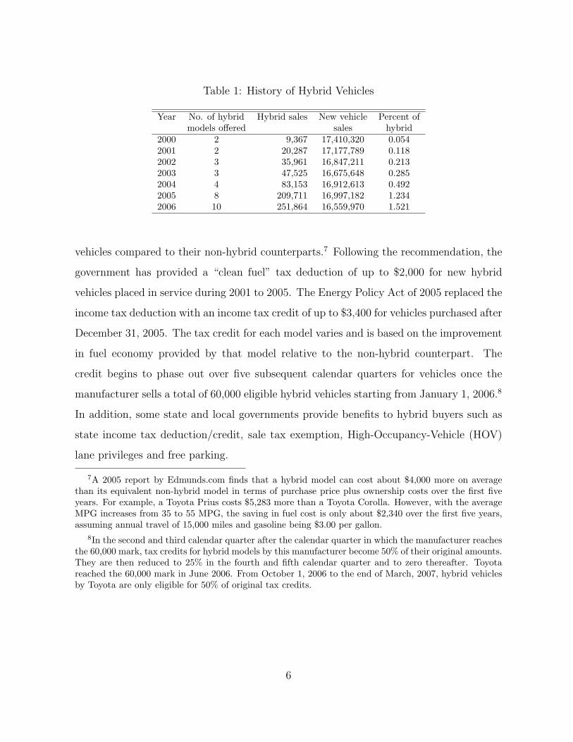
Table 1: History of Hybrid Vehicles

Year No. of hybrid Hybrid sales New vehicle Percent ofmodels offered sales hybrid

2000 2 9,367 17,410,320 0.0542001 2 20,287 17,177,789 0.1182002 3 35,961 16,847,211 0.2132003 3 47,525 16,675,648 0.2852004 4 83,153 16,912,613 0.4922005 8 209,711 16,997,182 1.2342006 10 251,864 16,559,970 1.521

vehicles compared to their non-hybrid counterparts.7 Following the recommendation, the

government has provided a “clean fuel” tax deduction of up to $2,000 for new hybrid

vehicles placed in service during 2001 to 2005. The Energy Policy Act of 2005 replaced the

income tax deduction with an income tax credit of up to $3,400 for vehicles purchased after

December 31, 2005. The tax credit for each model varies and is based on the improvement

in fuel economy provided by that model relative to the non-hybrid counterpart. The

credit begins to phase out over five subsequent calendar quarters for vehicles once the

manufacturer sells a total of 60,000 eligible hybrid vehicles starting from January 1, 2006.8

In addition, some state and local governments provide benefits to hybrid buyers such as

state income tax deduction/credit, sale tax exemption, High-Occupancy-Vehicle (HOV)

lane privileges and free parking.

7A 2005 report by Edmunds.com finds that a hybrid model can cost about $4,000 more on averagethan its equivalent non-hybrid model in terms of purchase price plus ownership costs over the first fiveyears. For example, a Toyota Prius costs $5,283 more than a Toyota Corolla. However, with the averageMPG increases from 35 to 55 MPG, the saving in fuel cost is only about $2,340 over the first five years,assuming annual travel of 15,000 miles and gasoline being $3.00 per gallon.

8In the second and third calendar quarter after the calendar quarter in which the manufacturer reachesthe 60,000 mark, tax credits for hybrid models by this manufacturer become 50% of their original amounts.They are then reduced to 25% in the fourth and fifth calendar quarter and to zero thereafter. Toyotareached the 60,000 mark in June 2006. From October 1, 2006 to the end of March, 2007, hybrid vehiclesby Toyota are only eligible for 50% of original tax credits.

6

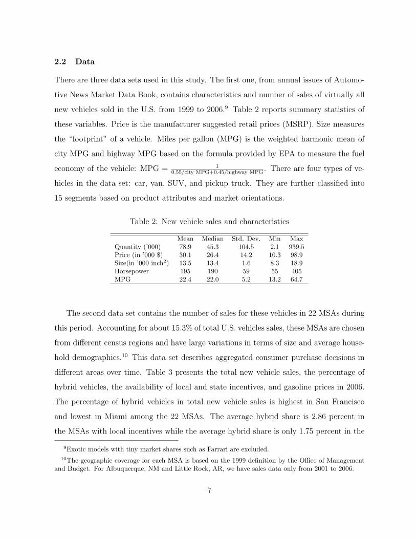
2.2 Data

There are three data sets used in this study. The first one, from annual issues of Automo-

tive News Market Data Book, contains characteristics and number of sales of virtually all

new vehicles sold in the U.S. from 1999 to 2006.9 Table 2 reports summary statistics of

these variables. Price is the manufacturer suggested retail prices (MSRP). Size measures

the “footprint” of a vehicle. Miles per gallon (MPG) is the weighted harmonic mean of

city MPG and highway MPG based on the formula provided by EPA to measure the fuel

economy of the vehicle: MPG = 10.55/city MPG+0.45/highway MPG

. There are four types of ve-

hicles in the data set: car, van, SUV, and pickup truck. They are further classified into

15 segments based on product attributes and market orientations.

Table 2: New vehicle sales and characteristics

Mean Median Std. Dev. Min MaxQuantity (’000) 78.9 45.3 104.5 2.1 939.5Price (in ’000 $) 30.1 26.4 14.2 10.3 98.9Size(in ’000 inch2) 13.5 13.4 1.6 8.3 18.9Horsepower 195 190 59 55 405MPG 22.4 22.0 5.2 13.2 64.7

The second data set contains the number of sales for these vehicles in 22 MSAs during

this period. Accounting for about 15.3% of total U.S. vehicles sales, these MSAs are chosen

from different census regions and have large variations in terms of size and average house-

hold demographics.10 This data set describes aggregated consumer purchase decisions in

different areas over time. Table 3 presents the total new vehicle sales, the percentage of

hybrid vehicles, the availability of local and state incentives, and gasoline prices in 2006.

The percentage of hybrid vehicles in total new vehicle sales is highest in San Francisco

and lowest in Miami among the 22 MSAs. The average hybrid share is 2.86 percent in

the MSAs with local incentives while the average hybrid share is only 1.75 percent in the

9Exotic models with tiny market shares such as Farrari are excluded.10The geographic coverage for each MSA is based on the 1999 definition by the Office of Management

and Budget. For Albuquerque, NM and Little Rock, AR, we have sales data only from 2001 to 2006.

7

Table 3: Hybrid sales and local incentives in 2006

MSA Number of Hybrid Percent in total Local incentive Gasolinehouseholds sales vehicle sales (start date) price $

Albany, NY 360,273 737 1.62 Income tax (03/04) 2.70Albuquerque, NM 319,922 763 2.37 Excise tax (07/04) 2.58Atlanta, GA 1,994,938 2,775 1.34 No 2.52Cleveland, OH 1,167,916 1,643 1.16 No 2.51Denver, CO 1,132,085 3,561 3.51 Income tax (01/01) 2.45Des Moines, IA 209,297 438 1.96 No 2.32Hartford, CT 704,130 1,535 2.00 Sales tax (10/04) 2.80Houston, TX 2,197,010 3,132 1.22 No 2.49Lancaster, PA 197,929 318 1.80 No 2.53Las Vegas, NV 713,397 1,340 1.32 No 2.62Little Rock, AR 250,142 436 1.50 No 2.48Madison, WI 185,657 917 4.88 No 2.55Miami, FL 1,706,995 2,322 0.87 HOV (07/03) 2.64Milwaukee, WI 682,896 1,340 1.99 No 2.59Nashville, TN 548,192 752 1.47 No 2.43Phoenix, AZ 1,585,544 3,254 1.53 No 2.51St. Louis, MO 1,100,071 1,526 1.30 No 2.40San Antonio, TX 739,674 1,022 1.25 No 2.41San Diego, CA 1,177,384 4,946 3.40 HOV (08/05) 2.85San Francisco,CA 2,871,199 20,162 7.02 HOV (08/05) 2.87Seattle, WA 1,529,146 5,732 3.82 Sales tax (01/05) 2.70Syracuse, NY 292,717 408 1.15 Income tax (03/04) 2.69

MSAs without local incentives.

Based on these market-level sales data, we estimate a linear regression to examine

the correlation between MSA characteristics and hybrid sales. The dependent variable

is the share of hybrid vehicles among the total sales of all new vehicles. Mean eduction

is the average education level of the household head in the MSA. Local incentive is a

dummy variable capturing whether there are state and local incentives available. Tax

credit is essentially a dummy variable for year 2006 in which federal tax credits replaces

tax discounts for hybrid buyers.

The coefficients of all the variables except the local incentive dummy are significant at

the 5% significance level (the standard errors are cluster standard errors where a cluster

is an MSA). All the variables have positive effects on hybrid sales. The regression results

8

Table 4: OLS regression of hybrid shares

Variable Para. Std. Err.Constant -9.495 1.396Mean income 0.252 0.093Gas price 0.835 0.107Mean education 0.575 0.141Trend 0.136 0.037Local incentive 0.255 0.209Tax credit 0.566 0.074No. of obs. 172R-squared 0.715

suggest that areas with higher gasoline prices have stronger hybrid demand. Consumers

with higher income and more education are more likely to buy hybrid vehicles. To the

extent that many consumers buy hybrids to make a statement about their conviction

of environmental protection, people with higher income and more education may have

more resources and awareness to do so. The coefficient on Trend captures the fact that

the demand for hybrids is stronger over time, ceteris paribus. The coefficient on Local

incentives is intuitively signed but insignificant.11 Tax credits, which represent stronger

government support than tax discounts available before 2006, do increase hybrid sales.

As discussed above, our first data set describes vehicle choices consumers face while

the second data set presents consumer purchase decisions at the aggregate level in the

22 MSAs. However, the link between household demographics and consumer choice is

missing. The third data set, the 2001 National Household Travel Survey (2001 NHTS),

helps relate household demographics to purchase decisions. The survey was conducted

by agencies of the Department of Transportation from March 2002 through May 2003.

This data set provides detailed household level data on vehicle stocks, travel behavior and

household demographics at the time of survey. There are 69,817 households and 139,382

vehicles in the data. Among all the surveyed households, 45,984 are from MSAs.

11If local incentives are set in response to unobserved local factors that affect hybrid vehicle purchases,the coefficient on local incentives cannot be interpreted as the effect of local incentives on hybrid vehicledemand.

9

Table 5: Average household demographics

All Households who purchaseNew Car Van SUV Pickup

Household size 2.55 2.88 2.67 3.81 3.02 2.84Renter 0.364 0.211 0.266 0.090 0.147 0.163Children dummy 0.336 0.402 0.328 0.696 0.499 0.352Age of household head 48.83 46.89 48.07 46.24 44.19 46.25Time to work (minutes) 17.90 20.92 20.49 19.75 19.73 24.00

Table 6: New vehicle purchase probability

Income (’000) Purchase probability< 15 0.0020[15, 25) 0.0440[25, 50) 0.1125[50, 75) 0.1728[75, 100) 0.1972≥ 100 0.2574All households 0.1304

Column 2 in Table 5 shows the means of several demographics for households living

in MSAs. Renter, a dummy variable, equals 1 for the households that living in rented

houses and 0, otherwise. Children dummy, also a dummy variable, is 1 for households

with children. Columns 3 to 7 present the means of household demographics for different

groups based on household vehicle choice. These conditional means provide additional

moment conditions in our estimation where we match the predicted moments from the

empirical model to these observed moments. As household incomes are categorized and

top-coded at $100,000, we provide the probability of new vehicle purchase for six income

groups in Table 6. In our estimation of the empirical model, these conditional probabilities

are matched by their empirical counterparts.

10

3 Empirical Model and Estimation

In this section, we discuss our empirical model and estimation strategy. Our empirical

model closely follows recent empirical literature on differentiated products (e.g., BLP,

Petrin (2002), Berry et al. (2004)). The empirical model includes both a demand side and

a supply side. Vehicle demand is derived from a random coefficient discrete choice model.

A household makes a choice among all new models and an outside alternative to maximize

household utility in each year. We use their aggregated decision outcomes (product sales

in this case) to recover consumer preference parameters. The supply side assumes that

multiproduct firms engage in Betrand competition (taking product choices as given). The

first-order conditions of firm profit maximization allow us to recover the marginal cost for

each product. In a counterfactual analysis, we then base the recovered marginal cost and

the oligopolistic supply curve to solve for new equilibrium prices. We discuss each part

separately.

3.1 Demand Side

Household’s utility from a product is a function of household demographics and product

characteristics. Let i denote a household and j denote a product. A household chooses

one product from a total of J models of new vehicles and an outside alternative in a given

year. The outside alternative captures the decision of not purchasing any new vehicle in

the current year. To save notation, we suppress the market index m and time index t,

bearing in mind the choice set can vary across markets and years. The utility of household

i from product j (in market m at year t) is defined as

uij = v(pij, Xj, ξj, yi, Zi) + εij, (1)

where pij is the price of product j for household i. The price is computed based on the

MSRP, the sales tax and federal income tax incentives for hybrid vehicles.12 Xj is a vector

12MSRPs, also known as “sticker prices”, are set by manufacturers and are generally constant acrosslocations and within a model year. Although individual transaction prices are desirable in the analysis

11

of observed product attributes, ξj the unobserved product attribute, yi the income of

household i, and Zi is a vector of household demographics. εij is a random taste shock

that has type one extreme value distribution. The specification of the first term in the

utility function is assumed to be:

vij = αipij

yi

+K∑

k=1

xjkβ̃ik + ξj. (2)

We allow α to vary according to the income group of the household. xjk is the kth product

attribute for product j. β̃ik is the random taste parameter of household i over product

attribute k, which is a function of household demographics including those observed by

econometrician (zir) and those that are unobserved (νik):

β̃ik = β̄k +R∑

r=1

zirβkr + νikβuk . (3)

The utility of the outside alternative (j = 0) is specified as

vi0 = Ziβ0 + νi0βu0 + εi0, (4)

where νi0, the unobserved household demographics, captures different valuations of the

outside alternative by different households due to heterogeneity in vehicle holdings and

transportation choices.

Based on the utility function, we can derive the aggregate demand function. Define θ

as the vector of all preference parameters. The probability that the household i chooses

choice j ∈ {0, 1, 2, ..., J} is

Prij = Pri(j|p, X, ξ, yi, Zi, θ) =

∫exp(vij)∑J

h=0 exp(vih)dF (νi), (5)

of automobile demand given that different consumers may pay different prices for the same model, thesedata are not easily available. MSRPs have been commonly used in this literature.

12

where p is the vector of prices of all products. νi is a vector of unobserved demographics

for household i. The market demand for choice j for a price vector p is then

qj = q(j|p, X, ξ, θ) =∑

i

Prij. (6)

3.2 Supply Side

The demand side parameters can be estimated without a supply side model. However, a

supply side model is needed for the counterfactual analysis where we solve for the prices in

a new equilibrium based on firms’ price-setting rules derived from the profit maximization

problem. Firms are assumed to engage in Betrand competition to maximize the period

profit from the whole U.S. market while taking the product mix as given.

The period total variable profit (total revenue minus total variable cost) of a multi-

product firm f is

πf =∑

j∈F(f)

[pjqj(p, θ)− vcj(qj)

], (7)

where F(f) is the set of products produced by firm f . pj is the price and qj is the sales

for product j. vcj is the total variable cost of product j.13

∑h∈F

[ph −mch(qj)

]∂qh(p, θ)

∂pj

+ qj(p, θ) = 0. (8)

The equilibrium price vector is defined, in matrix notation, as

p = mc(q) + ∆−1q(p, θ), (9)

13We do not consider the role of the CAFE constraints on firms’ pricing decision here. See Jacobsen(2007) for an examination of how firms, particularly U.S. firms underprice their fuel-efficient vehicles inorder to meet the CAFE standards. In recent years, the CAFE constraints have not been binding forToyota and Honda who produces the majority of the hybrid vehicles.

13

where the element of ∆ is

∆jr =

−∂qr

∂pjif product j and r produced by same firm

0 otherwise.(10)

Equation (9) underlies the pricing rule in a multiproduct oligopoly: equilibrium prices

are equal to marginal costs plus markups, ∆−1q(p, θ). The implied marginal costs can

be computed following mc = p − ∆−1q, where p and q are the observed prices and sales.

In a counterfactual analysis, the fixed point of equation (9) can be used to compute new

price equilibrium corresponding to a change in the demand equation q(p, θ), providing

that we know the relationship between mc and q. Constant marginal cost assumption has

been commonly used in recent literature on estimating automobile market equilibrium (for

example, Bresnahan (1987); Goldberg (1995)).14 If marginal costs are not constant with

respect to the total output level, the functional relationship between the two has to be

recovered in order to find new equilibrium prices in counterfactual scenarios.

3.3 Estimation

The preference parameters in the utility function are estimated by matching the predicted

market sales as shown in equation (6) with observed sales in each market. The predicted

market sales are computed based on a random sample of households from the 2000 Census

data while taking into account various government support programs for hybrid vehicles.

Because the federal incentives for hybrid vehicles are in the forms of income tax deduc-

tions or income tax credits, they may vary across households depending on household tax

liabilities: households with fewer tax liabilities tend to enjoy less tax benefit from buying

a hybrid vehicle. To figure out tax incentives for each household, we calculate household

income tax liabilities using NBER’s online software TAXSIM (version 8.0). TAXSIM takes

household income sources and other demographics from survey data as input and returns

14The constant marginal cost assumption does not reject the existence of economies of scale. A highfixed cost and constant marginal cost can still result in economies of scale.

14

tax calculations as output.15

To illustrate our estimation strategy, which exploits the fact that we observe the de-

mand for each product in many MSAs, we bring the market index m into the utility

function and write the utility function as

umij = δmj + µmij + εmij, (11)

where δmj, the mean utility of product j in market m, is the same for all the households

in market m. The mean utility from the outside alternative is normalized to zero. µmij is

the household specific utility. The mean utility is specified as follows

δmj = δj + Xmjγ + emj, (12)

where δj is a product dummy, absorbing the utility that is constant for all households

across the markets (including the utility derived from the unobserved product attributes

ξj).16 Xmj is a vector of product attributes that vary across MSAs. It includes dollars per

mile (DPM), which is the gasoline price in market m divided by the MPG of product j.

DPM captures the operating cost of the vehicle. emj is the part of the mean utility that

is unobserved to us.

mumij is the household specific utility. Following notations in equations (2) and (3),

the household specific utility is:

µmij = αipij

yi

+∑kr

xmjkzhirβ

okr +

∑k

xmjkνikβuk . (13)

The household specific utility for the outside alternative is defined by equation (4). Denote

the parameters in the mean utility as θ1 = {δj, γ}, and the parameters in the household

15TAXSIM and an introduction by Feenberg and Coutts (1993) are available athttp://www.nber.org/taxsim.

16Following equations (2) and (3), δj =∑

k xjkβ̄k +∑

kn xjkznβkn + ξj . Although the parameters fromthis equation can be estimated once we recover δj , they are not of our interest in this paper.

15

specific utility as θ2 = {α, βokr, β

uk , β0, β

u0 }.

In estimating the demand model, a key identification problem arises from the correla-

tion between the vehicle prices and unobserved product attributes, which are represented

by a latent variable ξj. Since better product attributes often command a higher price, fail-

ure to take into account the unobserved product attribute often leads to omitted variable

bias in the estimate of price coefficient, suggesting that consumers are less price sensitive

than they really are (Trajtenberg (1989); Berry et al. (1995); Petrin (2002); Goolsbee and

Petrin (2004)). A common, although strong, identification assumption is that the un-

observed product attribute is uncorrelated with observed product attributes. Similar to

Nevo (2001), we avoid invoking this assumption by using product dummies to absorb the

unobserved product attribute and observed product attributes that are constant across

MSAs.

We, nevertheless, make the assumption that the error term in the mean utility function,

emj, is uncorrelated with market-varying attributes, Xmj. Because we only observe vehicle

prices (i.e., MSRP) at the national level, emj may capture local price variations and

promotions. emj may also contain other unobservables such as driving conditions that

affect consumers’ vehicle preferences. If these local unobservables vary systematically with

vehicle fuel economy, the coefficient on DPM is biased downward, suggesting consumers are

less sensitive to vehicle fuel cost than what they really are.17 In the estimation, we include

interaction terms between MSA dummies and vehicle types, such as those between MSA

dummies and a dummy variable for hybrid models, to control for these local unobservables.

θ1 and θ2 can be estimated simultaneously by matching the predicted market shares

based on our demand model with observed market shares. However, the large number

of product dummies renders this approach impractical because the within-group demean-

ing method as a way to estimate fixed-effect models cannot be applied in this nonlinear

framework. Instead, we estimate the model following an iterative two-stage procedure.

17An example would be that dealers in an area with high gasoline prices may offer deeper discounts forfuel-inefficient vehicles than those in an area with low gasoline prices.

16

The first stage uses a contracting mapping technique to recover the mean utility δmj for

each product in each market as a nonlinear function of θ2. BLP shows that under some

mild conditions, for a given a θ2, there exists a unique vector of mean utility δmj that

equates the observed market shares in a given market to the predicated market shares.

For a given θ2, the unique vector of mean utilities for market m, δm, can be recovered

using a fixed point iteration:

δn+1m = δn

m + ln(Som)− ln[Sm(δn

m, θ2)], (14)

where n is the number of iterations; Som is the vector of observed market shares in market

m while Sm is the vector of predicted market shares.

The second stage is a simulated GMM with two sets of moment conditions that are

formed based on recovered mean utilities from the first stage for any given θ2. The first

set of moment conditions is from the exogeneity assumption in equation (12) that emj is

mean independent of Xmj. From equation (12), emj can be written as a function of θ1

and δmj, which is recovered as a function of θ2 from the first stage. Our first set moment

conditions M1 is based on:

E[emj(θ1, θ2)|Xmj

]= 0.

The second set, M2, includes 17 micro-moments which match the model predictions

to the observed conditional means from the 2001 NHTS as shown in Tables 5 and 6. For

example, we match the predicted probability of new vehicle purchase among households

with income less than $15,000 to the observed probability in the data.

E[Pri(j 6= 0)|(yi < 15, 000; δm(θ2), θ2, )

]= 0.002.

With an initial value of θ2, we recover δmj using the contraction mapping. We form

the objective function by stacking the two sets of moment conditions which are functions

of the initial value of θ2 and the recovered δmj as a function of θ2. The GMM estimators

17

θ̂1 and θ̂2 minimizes:

J = M(θ1, θ2)′WM(θ1, θ2) =

M1(θ1, θ2)

M2(θ2)

′ W1 0

0 W2

M1(θ1, θ2)

M2(θ2)

.

The procedure involves iteratively updating θ2 and then δmj to minimize the objective

function. We start with using the identity matrix as the weighting matrix to obtain

consistent initial estimates of the parameters and optimal weighting matrix. We then

estimate the model using the new weighting matrix.

With the estimation of the demand side, we can recover the marginal cost for each

model based on firms’ first order condition for profit maximization in equation (9). The

first order condition can also be used to simulate new equilibrium prices in the counterfac-

tual scenarios. We perform two sets of simulations for each counterfactual scenario. One

set employs constant marginal cost assumption and the other is based on the estimated

relationship between the marginal cost and production. Because U.S. domestic sales of a

model often do not coincide with total production of the model due to international trade

and data on model-level production are not readily available, we use vehicle sales as the

proxy for production in the case of non-constant marginal costs and specify the marginal

cost of model j as the following:

mcj = ωjρ + ζj, (15)

where ωj includes model attributes and U.S. sales. ζj is the error term which may include

production cost from unobserved product attributes and productivity shock as well.

An endogeneity problem arises in estimating the non-constant marginal cost function

given that sales are related to unobserved product attributes. To control for the endogene-

ity problem, we employ the commonly used identification assumption in the differentiated

product literature that unobserved product attributes are mean independent of observed

product attributes. Based on this assumption, valid instruments for vehicle sales are pro-

18

vided by the observed attributes of other products. These exclusion restrictions arise

naturally in a differentiated-product market, where the level of product differentiation is

an important factor in determining equilibrium price and quantity. However, the large

number of vehicles offered in the U.S. market yields more instruments than we can di-

rectly apply. We construct two “distance” measures for each product as parsimonious

instruments for vehicle sales following Li (2006). The distance measures reflect how dif-

ferentiated a product is from other products within the firm and outside the firm. The

measures are based on distances between two products in a Euclidean space where differ-

ent weights are applied to different dimensions of the product-characteristics space. The

weights are the coefficients of the corresponding product attributes in a hedonic price

regression.

4 Estimation Results

We first report parameter estimates and then use these estimates to calculate price elas-

ticities and implied markups for selected products. Table 7 presents the estimates of the

parameters in the mean utility as shown in equation (12). We include product fix effects

which absorb the part of the mean utility δmj that is constant across MSAs. The co-

efficient on DPM is negative and estimated precisely, reflecting that consumers’ vehicle

purchase decisions respond to the fuel cost from operating a vehicle. A vehicle with better

fuel efficiency hence smaller DPM is valued more than a less fuel-efficient vehicle, ceteris

paribus. The identification of this coefficient is based on the cross-MSA sales variation in

response to differences in gasoline prices across MSAs: a fuel-efficient vehicle should be

more popular in a high gasoline price area than otherwise, all else equal. The variable,

local support dummy, equals to 1 for the hybrid models in MSAs where local government

supports such as HOV lane privilege and free meter parking are available for hybrid pur-

chases. The coefficient on this variable is positive and significant, suggesting a positive

correlation between state and local incentives and the diffusion of hybrid vehicles.

The interaction terms between MSA dummies and the hybrid dummy capture unob-

19

served heterogeneity on hybrid demands that may arise from differences in dealer availabil-

ity and consumer attitudes toward hybrid vehicles. Based on these parameter estimates,

consumers in Seattle, San Francisco and San Diego have the strongest incentives to buy

hybrid vehicles. We include interactions terms between MSA dummies and vehicle type

dummies (i.e., car, SUV, van and pickup truck) to control for unobserved heterogeneity

in consumer preference for each type of vehicles across MSAs. For example, consumers

in MSAs with more snow and slippery driving conditions might prefer SUVs and pickup

trucks, which are often equipped with four-wheel-drive.

Table 7: Parameter estimates in the mean utility

Variables Para. Std. Err.Dollars per mile (DPM) -4.110 0.425Local support dummy 1.635 0.275MSA dummy * Hybrid dummy(base group: Albany, NY)Albuquerque, NM -1.477 1.469Atlanta, GA -1.171 0.517Cleveland, OH -1.816 0.533Denver, CO -2.625 0.521Des Moines, IA -0.244 0.504Hartford, CT -1.559 0.353Houston, TX -2.722 0.600Lancaster, PA -0.828 0.490Las Vegas, NV 0.367 0.650Little Rock, AR -2.387 1.405Madison, WI -0.206 0.538Miami, FL -0.384 0.468Milwaukee, WI -0.949 0.445Nashville, TN -0.759 0.478Phoenix, AZ -1.429 0.519St. Louis, MO -2.113 0.479San Antonio, TX -0.458 0.466San Diego, CA 0.443 0.484San Francisco,CA 0.708 0.428Seattle, WA 0.825 0.369Syracuse, NY -1.379 0.458MSA dummy * Segment dummy (84) YesProduct Fixed Effects (1619) Yes

In table 8, we present the estimates of the parameters in the household specific util-

20

ity defined by equation (13). These parameters capture consumer heterogeneity due to

observed and unobserved household demographics. The first four coefficients capture con-

sumer heterogeneity in preference for vehicle price. The coefficient for high income groups

being larger implies richer households are less price sensitive. The second four parameters

are for the interaction terms between household size and vehicle type dummies. These

interaction terms allow families with different household size to have different tastes for a

certain type of vehicle. A positive and significant coefficient estimate on the interaction

term between household size and van dummy means that the utility from a van increases

with household size, ceteris paribus. We also interact house tenure with vehicle type dum-

mies. The last three coefficients being negative and significant suggests that a household

in a rented house values van, SUVs and pickup trucks less than those living in their own

houses. The estimate of the term interacting the outside alternative with the children

dummy suggests that households with children value a new vehicle more than those with-

out. So do those households with a younger household head and those whose commuting

time is longer.

Table 8 then reports the estimates of eight random coefficients, which measure the

dispersion of heterogeneous consumer preference. These coefficients are the standard errors

of consumer preferences for the corresponding product attributes, while the means of

consumer preference are presented in table 7. For example, the preference parameter on

DPM has a standard normal distribution with mean -4.110 and standard error 2.250.

Therefore, 90 percent of the households have a preference parameter on DPM in the range

of [-7.823, 0.398]. The random coefficients ultimately break the independence of irrelevant

alternatives (IIA) property of standard logit models in that the introduction a new model

into the choice set will draw disproportionately more consumers to the new model from

similar products than from others.

Based on our demand and supply estimations, we compute demand elasticities with

respect to price and markups. The markup for product j is defined aspj−mcj

pj, where pj

and mcj are the price and the marginal cost of product j, respectively. Table 9 reports

21

Table 8: Parameter estimates in household specific utility

Variable Para. Std. Err.Price/Income if income ≤ 25,000 -43.308 3.545Price/Income if income ≤ 50,000 & income > 25,000 -39.714 2.790Price/Income if income ≤ 100,000 & income >50,000 -34.040 4.041Price/Income if income > 100,000 -27.263 9.249Household size * car dummy -1.340 0.572Household size * van dummy 5.629 0.407Household size * SUV dummy -1.362 0.626Household size * pickup dummy -0.293 1.540Rented house * car dummy -1.252 1.530Rented house * van dummy -14.461 3.233Rented house * SUV dummy -4.353 1.606Rented house * pickup dummy -7.841 4.434Education * hybrid dummy 0.312 0.828Children dummy * outside good -4.968 1.489Head age * outside good 0.078 0.029Travel time * outside good -0.086 0.025Random CoefficientHybrid dummy 1.495 0.224Log(miles per dollar) 2.250 0.537Log(horse power) 6.774 0.230Log(size) 1.495 0.224Car dummy 9.460 0.688Van dummy 26.479 1.795SUV dummy 4.901 0.621Pickup dummy 54.061 3.336Outside good 20.815 0.571

own price elasticities and markups for selected products in 2006. One obvious pattern

from this table is that within a vehicle class, the demand for cheaper products tends to

be more price sensitive.18 Among these 14 products, the two most expensive products,

Mercedes-Benz E class and Cadillac Escalade, have the highest markup of 21.80% while

the cheapest product, Ford Escort, has the lowest markup of only 8.62%. Interestingly,

among three hybrid models, Toyota Prius, although being the cheapest, has the smallest

price sensitivity and highest markup.19 both elasticities and markups. Among all the

18Contrary to our finding from the random coefficient specification, a logit model would predict thatexpensive products tend to be more price elastic.

19To the extent that some consumers advertise themselves as environmentalists by driving hybrid ve-hicles, Prius’s distinct appearance makes the model less substitutable than other hybrid models such as

22

Table 9: Price elasticities and markups

Products in 2006 Price Elasticities Markups (in %) U.S. SalesCARSFord Focus 15,260 -13.75 8.62 177,006Toyota Camry 19,855 -9.85 12.12 417,104BMW 325 31,595 -7.69 14.38 120,180Mercedes-Benz E class 51,825 -5.23 21.80 50,195VANSKia Sedona 23,665 -12.16 9.13 57,018Honda Odyssey 25,895 -8.27 12.98 177,919PICKUPSFord Ranger 18,775 -14.99 7.96 92,420Toyota Tacoma 28,530 -6.92 16.85 178,351SUVSHonda CR-V 22,145 -12.22 9.36 170,028Jeep Grand Cherokee 28,010 -11.11 10.83 139,148Cadillac Escalade 57,280 -6.15 21.80 62,206HYBRIDSToyota Prius 22,305 -7.61 16.39 106,971Toyota Camry Hybrid 25,900 -10.87 12.17 31,341Toyota Highlander 34,430 -8.10 15.51 31,485

products, the sales weighted average price elasticity is -10.91 while the average markup is

12.17%.20

Table 10 reports the estimation results for the marginal cost function. Bearing in

mind that we use U.S. sales as the proxy for total production in order to estimate the

relationship between the marginal cost and total production at the model level. Due to

the fact that imported models can be very poor proxies for their total production, we

use only the models produced in the U.S. to estimate the marginal cost function. These

models include those produced by the Big Three and foreign transplants in the U.S. as

well. Columns (1) and (2) report coefficient estimates assuming that marginal costs do not

change with quantity produced. All the listed coefficient estimates are intuitively signed

Honda Civic which has the same look as the non-hybrid Civic as suggested by Kahn (2008).20Our estimate of average markup is closest to Petrin (2002)’s estimate of 16.7 percent which is based

on vehicles sold from 1981 to 1993 including cars, vans and pickup trucks. Goldberg (1995) recovers amuch larger estimate of 38 percent for cars from 1983 to 1987 while the average benchmark markup inBLP is estimated as 23.9 percent for cars sold between 1971 and 1990. We have about 200 models eachyear while Petrin (2002) 185 models, Goldberg (1995) and BLP each have about 110 models per year.

23

and all of them except the coefficient on size are significant at the 10% significance level.

Table 10: Marginal cost function

Variable Constant MC-OLS Non-constant MC-OLS Non-constant MC-IVParameter Std. Err. Parameter Std. Err. Parameter Std. Err.

(1) (2) (3) (4) (5) (6)Log (sales in 10,000) -0.763 -0.077 -1.078 -0.432Constant -6.890 2.522 -6.875 2.386 -6.868 2.410Size 0.107 0.176 0.270 0.168 0.337 0.192HP 0.473 0.032 0.450 0.030 0.440 0.033MPG 1.078 0.494 1.337 0.468 1.444 0.495Weight 0.372 0.067 0.345 0.064 0.334 0.066Segment dummies (14) Yes Yes Yes Yes Yes YesYear dummies (7) Yes Yes Yes Yes Yes YesObs. 873 873 873R-squared 0.908 0.917

Columns (3) and (4) are the OLS results for non-constant marginal costs while the

results in columns (5) and (6) are from the GMM estimation where the endogeneity of

log(sales) is controlled for using product distance measures as instruments. The coeffi-

cient estimates on log(sales) in both regressions being negative means that the marginal

cost is decreasing, although at a smaller rate, as production expands.21 Compared to

the instrument variable regression, the OLS underestimates the coefficient on log(sales),

suggesting a smaller reduction in marginal cost as total production goes up. Because

better unobserved product attributes imply a higher marginal cost and at the same time,

stronger sales, the observed product attributes bias economies of scale downward in the

OLS regression.

21The J-statistics for over-identification test in the GMM estimation is 0.784, implying a p-value of0.367. We assume that the relationship between the marginal cost and production for hybrid models isthe same as that for non-hybrid models because we only observe two hybrid models produced in the U.S.in our data. We also estimate the model with a second order of log(sales). The coefficient on that ispositive but not significantly different from zero. This may suggest that firms have not been operating atthe production level that exhibits increasing marginal cost during the period under study.

24

5 Simulations

In this section, we conduct counterfactual simulations to address the effect of rising gaso-

line prices and federal tax incentives on the diffusion of hybrid vehicles. We then conduct

simulations to compare the current income tax incentive program with a rebate program

in terms of their cost-effectiveness and their effects on industry profits. We solve new

equilibrium prices under each scenario based on the estimates of demand parameters and

product marginal costs, assuming firms’ objectives are to maximize the total period profit

from the whole U.S. market. We then estimate new sales for the 22 MSAs under new

equilibrium prices. Before presenting the results, it is worthwhile to note that our simula-

tions assume the product offerings would stay the same under different scenarios.22 To the

extent that both the run-up of the gasoline price and the presence of federal tax incentives

strengthen consumer incentives to purchase hybrid vehicles and therefore increase firms’

incentive to offer more hybrid models, our static analysis would underestimate the true

effects of these two factors.

5.1 Gasoline Prices

Understanding how vehicle choice decisions of consumers respond to changes in gasoline

prices has important implications for policies that aim to address energy security and

environmental problems related to gasoline consumption. Based on our model estimations,

we investigate to what extent the recent run-up of gasoline prices contributes to the

diffusion of hybrid vehicles. To that end, we simulate what would have happened if

gasoline prices from 2000 to 2006 had been the same as those in 1999 level in each of the

22 MSAs.

Columns (1) to (3) in able 11 presents the effects of gasoline price changes on prices

of five hybrid models and their non-hybrid counterparts in 2006. The national average

22The decision of product choice, although an interesting topic, is out of scope of this paper. A seriousapproach to this topic involves modeling a dynamic game where the model should contend with severalkey facts about the auto industry: the industry consists of several big players that act strategically, eachof them produces multiple products, and products are differentiated.

25

Table 11: The effect of gas price change on vehicle prices and sales

Models in 2006 Price New Change Sales in New Changein 2006 $ Price in % 22 MSAs Sales in %

(1) (2) (3) (4) (5) (6)Hybrid ModelsFord Escape Hybrid 29,140 28,734 -1.39 3,862 3,798 -1.65Honda Civic Hybrid 22,400 21,662 -3.29 7,232 5,883 -18.65Honda Accord Hybrid 31,540 31,031 -1.61 1,210 1,060 -12.41Toyota Highlander Hybrid 34,430 33,319 -3.23 7,594 7,552 -0.55Toyota Prius 22,305 21,407 -4.03 26,625 21,262 -20.14Non-hybrid CounterpartsFord Escape 21,745 22,139 1.81 17,276 21,899 26.76Honda Civic 17,660 17,514 -0.83 60,112 56,709 -5.66Honda Accord 21,725 21,750 0.12 69,852 70,632 1.12Toyota Highlander 26,535 26,841 1.15 15,684 16,789 7.05Toyota Corolla 15,485 15,428 -0.37 74,928 74,868 -0.08

gasoline price was $1.35 in 1999 and $2.53 in 2006, both in 2006 dollars.23 If gasoline

prices had stayed at the 1999 level, the five selected hybrid models in 2006 would have

been 1.39 to 4.03 percent cheaper as shown in column (3) because they would have been

in lower demand given that their saving in fuel cost would be smaller. For their non-

hybrid counterparts, the changes in prices are smaller in magnitude. The price of Ford

Escape, Honda Accord and Toyota Highlander would have been higher with the gasoline

price staying at the 1999 level because they would have been in stronger demand while

two more fuel-efficient vehicles, Honda Civic and Toyota Corolla, would have been slightly

cheaper.

Columns (4) to (6) show the effect of gasoline price changes on sales. The decrease in

sales in the 22 MSAs for the five hybrid models ranges from 0.55 to 20.14 percent have

the gasoline price stayed at the 1999 level. The effect on the most efficient hybrid models,

Toyota Prius is most significant because buyers of this model are likely to be more sensitive

to gasoline prices. On the other hand, without the gasoline price increase in 2006, the

sales of regular Ford Escape and Toyota Highlander would have increased by 26.76 and

23The average gasoline price in the 22 MSAs weighted by vehicle sales was $1.53 in 1999 and $2.60 in2006.

26

7.05 percent, respectively while that of Honda Civic would drop by 5.66 percent.

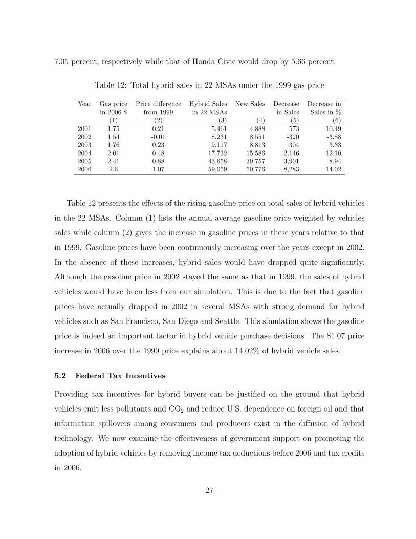
Table 12: Total hybrid sales in 22 MSAs under the 1999 gas price

Year Gas price Price difference Hybrid Sales New Sales Decrease Decrease inin 2006 $ from 1999 in 22 MSAs in Sales Sales in %

(1) (2) (3) (4) (5) (6)2001 1.75 0.21 5,461 4,888 573 10.492002 1.54 -0.01 8,231 8,551 -320 -3.882003 1.76 0.23 9,117 8,813 304 3.332004 2.01 0.48 17,732 15,586 2,146 12.102005 2.41 0.88 43,658 39,757 3,901 8.942006 2.6 1.07 59,059 50,776 8,283 14.02

Table 12 presents the effects of the rising gasoline price on total sales of hybrid vehicles

in the 22 MSAs. Column (1) lists the annual average gasoline price weighted by vehicles

sales while column (2) gives the increase in gasoline prices in these years relative to that

in 1999. Gasoline prices have been continuously increasing over the years except in 2002.

In the absence of these increases, hybrid sales would have dropped quite significantly.

Although the gasoline price in 2002 stayed the same as that in 1999, the sales of hybrid

vehicles would have been less from our simulation. This is due to the fact that gasoline

prices have actually dropped in 2002 in several MSAs with strong demand for hybrid

vehicles such as San Francisco, San Diego and Seattle. This simulation shows the gasoline

price is indeed an important factor in hybrid vehicle purchase decisions. The $1.07 price

increase in 2006 over the 1999 price explains about 14.02% of hybrid vehicle sales.

5.2 Federal Tax Incentives

Providing tax incentives for hybrid buyers can be justified on the ground that hybrid

vehicles emit less pollutants and CO2 and reduce U.S. dependence on foreign oil and that

information spillovers among consumers and producers exist in the diffusion of hybrid

technology. We now examine the effectiveness of government support on promoting the

adoption of hybrid vehicles by removing income tax deductions before 2006 and tax credits

in 2006.

27

Table 13: The effect of tax incentives on selected hybrid models

With Incentives Remove IncentivesPrice Sales in Tax Price Decrease Sales Decrease

(in 2006 $) 22 MSAs Benefit in 2006 $ in % in %(1) (2) (3) (4) (5) (6) (7)

2005 ModelFord Escape Hybrid 28,330 2,918 521 210 0.74 181 6.20Honda Civic Hybrid 20,815 4,836 513 186 0.89 316 6.53Honda Accord Hybrid 31,489 3,146 477 216 0.69 168 5.33Toyota Highlander Hybrid 33,476 3,366 418 215 0.64 142 4.21Toyota Prius 22,106 25,528 517 207 0.93 1,378 5.402006 ModelFord Escape Hybrid 29,140 3,862 2,472 974 3.34 1,009 26.13Honda Civic Hybrid 22,400 7,232 2,067 727 3.24 1,591 22.00Honda Accord Hybrid 31,540 1,210 550 245 0.78 68 5.61Toyota Highlander Hybrid 34,430 7,594 1,868 852 2.47 1,406 18.52Toyota Prius 22,305 26,625 2,994 1,081 4.85 9,046 33.98

Table 13 presents the effects of income tax incentives on both prices and sales of several

selected hybrid models in 2005 and 2006. Column (1) shows the price of each model in

2006 dollars and column (2) gives the total sales in the 22 MSAs. Column (3) lists the

average tax benefit received by buyers of each model. In 2005, the $2,000 tax deduction

yields $521 income tax return for Ford Escape hybrid buyers on average. In 2006, hybrid

buyers are eligible for up to $2,600, $2,100, $650 and $3,150 tax credit for the purchase

of a Ford Escape hybrid, Honda Civic hybrid, Honda Accord hybrid and Toyota Prius,

respectively. The tax credit program is more generous for most hybrid models than the

tax reduction program. For example, buyers of Ford Escape hybrid on average obtain

$2,472 income tax return for their purchase in 2006, comparing to only $521 in 2005.

Without tax incentives, both prices and sales of these hybrid models would be reduced.

The supply price of a 2005 Ford Escape hybrid would be $210 lower as shown in column

(4). Comparing with the $521 tax benefit received by an average buyer, it suggests that

buyers capture about 60% of the government subsidy and the supplier about 40%. This

finding also holds for other hybrid models based on average tax benefits received by buyers

28

in column (3) and price decreases in the absence of government subsidy in column (4).24

The effect of tax incentives on hybrid vehicle sales in 2005 is less than 7% for the five

hybrid models shown in the table. However, the effect of more favorable tax incentives

in 2006 is much more significant: for 2006 Toyota Prius, about 34% of its sales can be

attributed to the tax credit policy in place.

Table 14: The effect of tax incentives on hybrid adoption from 2001 to 2006

Year Total Subsidy Subsidy per Hybrid Sales Sales w/o Sales Decrease(in 2006 $1,000) vehicle (in 2006 $) in 22 MSAs Incentives in %

(1) (2) (3) (4) (5)2001 3,489 639 5,461 5,014 8.192002 5,023 610 8,231 7,558 8.182003 4,966 545 9,117 8,346 8.462004 9,408 531 17,732 16,476 7.082005 21,435 491 43,658 41,387 5.202006 143,650 2,432 59,059 43,157 26.93

Table 14 presents the effect of tax incentives on total hybrid sales in the 22 MSAs from

2001 to 2006. Column (1) lists the total government subsidy for hybrid vehicle purchases

over the period. Column (2) presents average tax returns received by hybrid buyers in

2006 dollars. They are decreasing from 2001 to 2005 due to two facts. First, while the

tax deduction is kept at $ 2,000, the inflation is about 14% over this period. Second, the

number of households subject to Alternative Minimum Tax (AMT) increases significantly.

These households are not eligible for the tax benefit when buying hybrid vehicles. In 2006,

government support, in the form of tax credits, is much stronger: the tax benefit received

by each hybrid buyer is $2,432 on average. 26.93% of the total hybrid sales in the 22

24Our estimates show that buyers of Toyota Prius in 2006 capture about 65% of total federal taxincentives. Sallee (2008) estimates that buyers of 2006 Toyota Prius get at least 73% of total tax subsidiesusing detailed retail price data. In order to explain the finding that consumers capture the significantmajority of the benefit from federal tax subsidies in the case of Toyota Prius, whose production wascapacity constrained in 2006, he suggests a model where current vehicle prices influence future demand(e.g., due to goodwill). Allowing the intertemporal price effect in our model would intuitively increasethe percentage of benefit captured by consumers. Moreover, allowing decreasing marginal cost as we doin our following analysis would also generate the case where consumers capture a higher percentage oftax incentives.

29

MSAs could be explained by tax credits, comparing to less than 10% in previous years.

It is interesting to note that hybrid sales, although smaller, would still be increasing over

time even without tax incentives.

In 2005, U.S. motor gasoline consumption was 9.16 million barrels per day, account-

ing for about 45% of total U.S. petroleum consumption. Total CO2 emission from motor

vehicle usage was 3.78 million tons per day.25 Table 15 presents total reductions in CO2

emission and gasoline consumption in the U.S. over vehicle lifetime (15 years) assuming

annual travel of 12,000 miles per vehicle. These reductions arise from the increased sales of

hybrid vehicles induced by income tax incentives from 2001 to 2006. Given the small num-

ber of hybrid models available and small market share of hybrid vehicles, these reductions

have been inconsequential compared to total CO2 emission and gasoline consumption.

Nevertheless, the reductions in CO2 emission and gasoline consumption will become more

significant with ever increasing number of hybrid models on the market.

Table 15: Total reductions in gas consumption and CO2 emission over vehicle lifetime

Year CO2 Reduction Gasoline Reductionin million tons in million barrels

2001 0.11 0.262002 0.19 0.452003 0.18 0.422004 0.42 1.002005 0.68 1.622006 5.14 12.24

5.3 Tax Credit Versus Rebate

In both income tax deduction and income tax credit programs, households with lower

income hence lower income tax lability may not be eligible for the maximum possible

incentives. However, these household should be more responsive to tax incentives given

that they tend to be more price sensitive. This suggest a rebate program that allows

25Assuming consumption of one gallon gasoline generates 19.594 pounds of CO2.

30

equal subsidy across buyers of the same hybrid model may be more cost-effective.26 In

this section, we compare the income tax credit program with a rebate program, which

distributes equal subsidy across households who purchase the same hybrid model and are

not subject to AMT. 27

We also examine the effect of the rebate program on industry profit. With the same

amount of government spending, the increase in hybrid prices due to subsidy may be higher

in the tax credit program than in the rebate program given that high-income households

(less price sensitive) tend to receive more income tax benefits than low-income households

under the tax credit program. Therefore, the income tax programs may be more favorable

to auto manufacturers than the rebate program.

Table 16: Comparison of the tax credit program with a rebate program in 22 MSAs

Average MPG Total Subsidy Total Variable Profit Hybrid Salesin 22 MSAs (in 2006 $Million) (in 2006 $Million) in 22 MSAs

Baseline: Current Tax Credit ProgramTax Credit Program 23.19 143.65 8,268.57 59,059Rebate Program 23.19 138.69 8,266.97 58,567Difference 0 -4.96(-3.5%) -1.60 -492

Baseline: Increase Tax Credits by $1,000Tax Credit Program 23.34 269.84 8,275.54 80,517Rebate Program 23.34 249.87 8,271.91 79,009Difference 0 -19.97(-7.4%) -3.63 1,508

Table 16 shows the difference between the income tax credit program and the rebate

program in terms of total government subsidy and total industry variable profit. Under

the current tax credit program, the average MPG of new vehicles sold in 2006 is 23.19.

To reach the same average fuel-efficiency, the rebate program would cost 138.69 million

dollars in government revenue, comparing to 143.65 million dollars under the tax credit

26Another benefit of such a rebate program is analogous to that in income transfer from high-incomehouseholds to low-income households, which can be measured by changes in total consumer welfare. Wedo not quantify this benefit here.

27In recent years, more and more households in the top income quartile have been subject to AMT,which disqualifies these household for the tax incentives. In the tax rebate program, we assume thathouseholds subject to AMT are not eligible for the rebate, either.

31

program. Meanwhile, total industry variable profit from the 22 MSAs, defined as total

revenue minus total variable costs, would decrease slightly in the rebate program. Even

thought both programs reach the same level of average fuel-efficiency, there are slightly

fewer hybrid models sold in the rebate program, reflecting a stronger demand from low-

income households for Toyota Prius and Honda Civic, two cheapest and most fuel-efficient

hybrid models. The rebate program would save about 3.5% in government subsidy. The

small magnitude is mainly due to the fact that under the current tax credit program,

only families with low income are not able to enjoy full tax incentives due to their low

tax liabilities and that the proportion of these households purchasing new vehicles is

very small. However, if the tax credit were to be increased or income tax credits for

other energy-efficient products are to be considered simultaneously in consumers’ vehicle

purchase decisions, more households would be constrained by their tax liabilities in getting

tax benefit from purchasing hybrid vehicles. Therefore, the rebate program would exhibit

a stronger advantage over the tax credit program. The difference between a more generous

tax credit program and a tax rebate program is shown in the second panel of the table

where we increase the tax credit for each hybrid model by $1,000.28 The average fuel-

efficiency increases to 23.34 MPG and the number of hybrid models sold increases to

80,517 with higher tax credits. For the average MPG of new vehicles to reach 23.34, the

rebate program would need 249.87 instead of 269.84 million dollars. This represents a

7.4% reduction in government subsidy to hybrid vehicle buyers.

5.4 Non-constant Marginal Costs

In this section, we investigate the robustness of our previous findings with respect to

the assumption of marginal costs. To that end, we conduct simulations based on our

estimation of the non-constant marginal cost function. One caveat of these simulation

results is that the marginal cost function is estimated using U.S. sales as proxies for total

28The Energy Policy Act of 2005 includes tax credits for many types of energy-efficient products. Themaximum amount of credit for qualified home improvements combined is $500 during the two year periodof 2006 and 2007. Moreover, a tax credit, up to $2,000, is available for qualified solar energy systems.

32

model production. Although in the estimation of the marginal cost function, we use

only domestically produced models (their U.S. sales may be good proxies for their total

production), we have to use U.S. sales for all the models as proxies for their total output

levels in the simulations due to the lack of production data. To the extent that U.S. sales

of imported models account for a smaller share of their total production than domestically

produced models, the simulation results for imported models overestimate the reduction

in their marginal costs from the increased sales given that the marginal cost function

decreases at a decreasing rate with the output level.

Table 17 compares the effects of the recent run-up in gasoline prices on hybrid vehicle

demand under two different scenarios of marginal costs. The first two columns are the

observed prices and sales in 22 MSAs. Columns (3) and (4) are the simulated prices and

sales for the case of constant marginal costs while columns (5) and (6) present simulated

prices and sales for the case of non-constant marginal costs had gasoline prices stay at

the 1999 level. The comparison between columns (4) and (6) shows that the effect of the

increase in gasoline prices on sales is stronger in case of non-constant marginal cost because

the larger sales of hybrid models due to higher gasoline prices reduce their marginal costs,

which in turn pushes the sales even larger. The same reason, however, causes the price

increases of hybrid models due to higher gasoline price to be smaller in the case of non-

constant marginal costs as shown in columns (3) and (5).

Table 17: Comparison of the effects of gasoline prices

Hybrid Models Observed Constant MC Non-constant MCin 2006 Price in Sales in Price in Sales in Price in Sales in

2006 $ 22 MSAs 2006 $ 22 MSAs 2006 $ 22 MSAs(1) (2) (3) (4) (5) (6)

Ford Escape 29,140 3,862 28,734 3,798 28,771 3,781Honda Civic 22,400 7,232 21,662 5,883 21,926 5,391Honda Accord 31,540 1,210 31,031 1,060 31,098 1,019Toyota Highlander 34,430 7,594 33,319 7,552 33,463 7,117Toyota Prius 22,305 26,625 21,407 21,262 21,674 19,411

Table 18 compares the effects of gasoline price changes and tax incentives on total

33

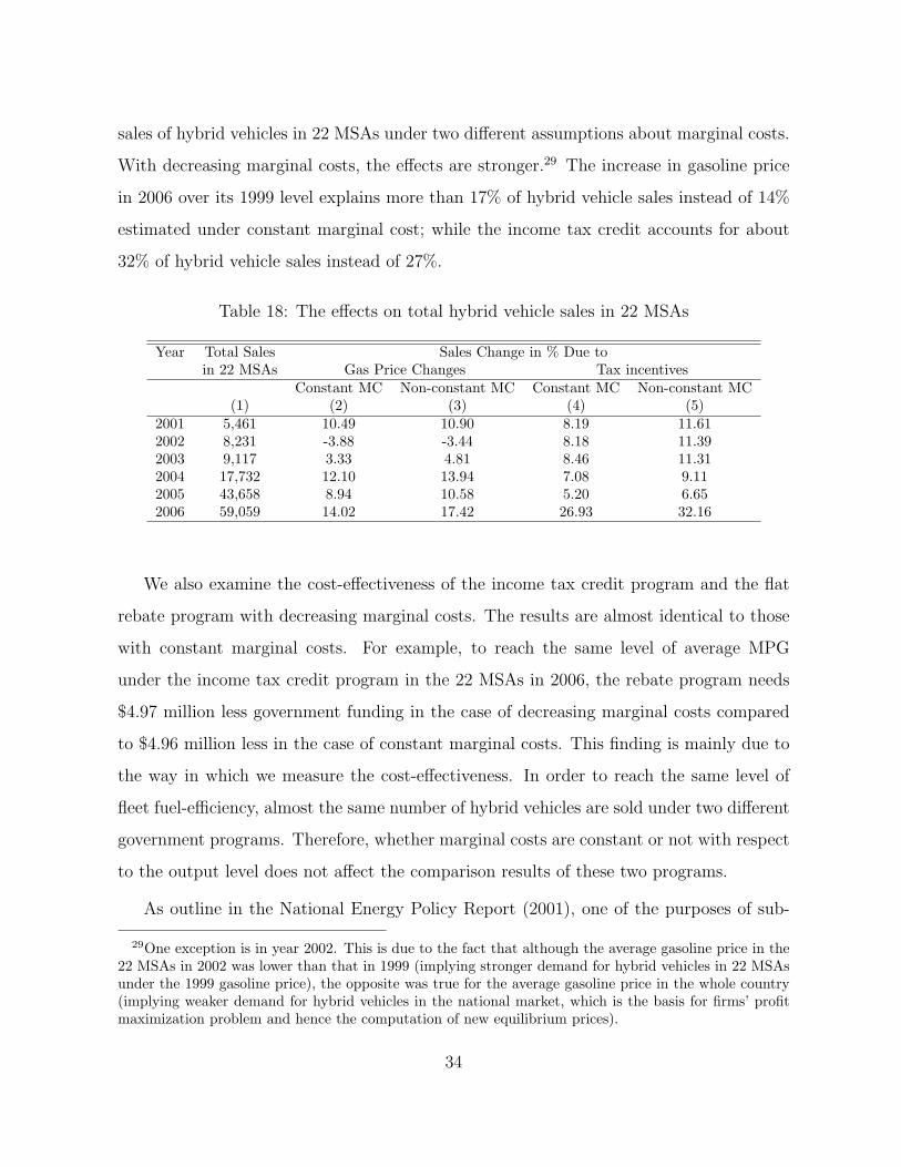
sales of hybrid vehicles in 22 MSAs under two different assumptions about marginal costs.

With decreasing marginal costs, the effects are stronger.29 The increase in gasoline price

in 2006 over its 1999 level explains more than 17% of hybrid vehicle sales instead of 14%

estimated under constant marginal cost; while the income tax credit accounts for about

32% of hybrid vehicle sales instead of 27%.

Table 18: The effects on total hybrid vehicle sales in 22 MSAs

Year Total Sales Sales Change in % Due toin 22 MSAs Gas Price Changes Tax incentives

Constant MC Non-constant MC Constant MC Non-constant MC(1) (2) (3) (4) (5)

2001 5,461 10.49 10.90 8.19 11.612002 8,231 -3.88 -3.44 8.18 11.392003 9,117 3.33 4.81 8.46 11.312004 17,732 12.10 13.94 7.08 9.112005 43,658 8.94 10.58 5.20 6.652006 59,059 14.02 17.42 26.93 32.16

We also examine the cost-effectiveness of the income tax credit program and the flat

rebate program with decreasing marginal costs. The results are almost identical to those

with constant marginal costs. For example, to reach the same level of average MPG

under the income tax credit program in the 22 MSAs in 2006, the rebate program needs

$4.97 million less government funding in the case of decreasing marginal costs compared

to $4.96 million less in the case of constant marginal costs. This finding is mainly due to

the way in which we measure the cost-effectiveness. In order to reach the same level of

fleet fuel-efficiency, almost the same number of hybrid vehicles are sold under two different

government programs. Therefore, whether marginal costs are constant or not with respect

to the output level does not affect the comparison results of these two programs.

As outline in the National Energy Policy Report (2001), one of the purposes of sub-

29One exception is in year 2002. This is due to the fact that although the average gasoline price in the22 MSAs in 2002 was lower than that in 1999 (implying stronger demand for hybrid vehicles in 22 MSAsunder the 1999 gasoline price), the opposite was true for the average gasoline price in the whole country(implying weaker demand for hybrid vehicles in the national market, which is the basis for firms’ profitmaximization problem and hence the computation of new equilibrium prices).

34

sidizing hybrid vehicle purchase is to help manufacturers achieve economies of scales and

reduce the production cost of hybrid vehicles. From the marginal cost function estimation,

we find that the marginal cost of vehicle production decrease with respect to output.30

Based on the marginal cost function, we can examine the extent to which government

support programs reduce the variable cost of hybrid vehicle production.31

Table 19 reports the reduction in the average variable cost (AVC) of five of the hybrid

models in 2006 brought about by the federal income tax credit program. Columns (3)

and (4) are total U.S. sales for each model with and without the income tax incentive,

respectively. The increase in U.S. sales due to the tax incentive ranges from 15% to 30%.

The last column reports the reduction in AVCs from the increases in sales. The production

of Toyota Prius enjoyed the largest reduction in the AVC due to the largest increase in

sales among these hybrid models. The results show that the $3,000 income tax credit on

the purchase of a Prius brought its AVC down by $421 in 2006.

Table 19: Reductions in the average variable cost for selected models

Year Hybrid Model Price in U.S. Sales U.S. Sales Reduction in2006 $ w/o Subsidy AVC in $

(1) (2) (3) (4) (5)2006 Ford Escape 29,140 19,375 15,321 2242006 Honda Civic 22,400 31,253 23,401 2892006 Honda Accord 31,540 5,598 5,268 412006 Toyota Highlander 34,430 31,485 25,709 2032006 Toyota Prius 22,305 106,971 71,694 421

Table 20 presents the decreases in the variable cost of hybrid vehicles over time due

to the federal income tax incentive programs. Columns (1) to (3) report, respectively,

the weighted average price, subsidy, and reduction in the AVC for hybrid vehicles in each

30Because most of the hybrid models are imported and their U.S. sales may not be good proxies fortheir total production, we are not able to estimate a separate relationship between the marginal cost andthe output level for hybrid vehicles.

31Given the high fixed cost in auto manufacturing, economies of scale can still arise even if the marginalcost of production is constant. However, without observing the fixed cost, we are not able to estimate thedecrease in the average cost of production induced by the federal tax incentive programs. Our estimateson the decrease in variable costs provide a lower bound for that.

35

Table 20: Reductions in the variable cost for all hybrid models

Year Average Price per Subsidy per Reduction U.S. Sales Reduction in totalHybrid Vehicle Hybrid Vehicle in AVC of Hybrids variable cost

in 2006 $ in 2006 $ in 2006 $ in million $(1) (2) (3) (4) (5)

2001 20,210 639 50 20,282 1.022002 19,918 610 57 35,961 2.062003 19,497 545 54 44,773 2.432004 19,294 531 56 82,555 4.612005 23,553 491 47 204,828 9.562006 23,849 2,432 309 251,633 77.87

year from 2001 to 2006. The weights are the observed sales of each hybrid model. An

average subsidy of $639 per hybrid vehicle yielded a $50 average reduction in the AVC in

2001 while an average subsidy of $2,432 achieved a $309 average reduction in the AVC of

hybrid models in 2006. Column (5) gives the total reduction in the total variable cost of

all hybrid models in each year brought about by the tax incentive programs. The results

show that the income credit program cut down the total variable cost of all hybrid vehicles

by nearly 78 million dollars in 2006.

6 Conclusion

With rising gasoline prices, unstable petroleum supplies, and growing concern about global

climate change and pollution, support for curbing U.S. fuel consumption has increased dra-

matically in recent years. The hybrid technology is considered as one promising solution

to energy security and environmental protection. To promote consumer adoption of hy-

brid vehicles, the U.S. government has been providing hybrid vehicle buyers income tax

incentives to offset the significantly higher cost of hybrid vehicles relative to their non-

hybrid counterparts. In this paper, we analyze the determinants in the demand for hybrid

vehicles, paying particular attention to the effect of rising gasoline prices and income tax

incentives. We also investigate the cost-effectiveness of the current income tax credit

program by comparing it to a hypothetical rebate program.

36

We find that the gasoline price is indeed an important factor in hybrid vehicle purchase

decisions. If the gasoline price in 2006 have stayed at the 1999 level ($1.53 instead of

$2.60 on average at the 22 MSAs), hybrid vehicle sales in 2006 would have been 14%

less. Our results confirm that recent increases in gasoline prices contribute significantly

to the increasing market share of hybrid vehicles. Moreover, the availability of income

tax incentives is also an important element in the demand for hybrid vehicles. Income

tax deductions explain about 5-9% of hybrid vehicle sales from 2001 to 2005 while more

generous income tax credits in 2006 account for about 27% of hybrid vehicles sales. These

findings suggest that in the absence of significant reduction in production costs hence

prices of hybrid vehicles, both high gasoline prices and continuous government support

may be necessary for further diffusion of hybrid vehicles.

Another finding is that a rebate program that offers enhanced incentives for low-income

households compared to the current income tax credit program costs less government

revenue in achieving the same average fuel-efficiency of new vehicles. The advantage of a

rebate program over an income tax credit program increases with the level of government

support. For example, we find that if current tax credits for hybrid models were to be

increased by $1,000, a rebate program that achieves the same average fuel-efficiency would

cost more than 7% less in government revenue. Although current government support for

consumers to adopt energy-efficient products mainly takes the form of income tax credits,

our finding calls for wider adoption of flat subsidy programs in future legislations that aim

to promote energy conservation and environmental protection.

37

References

Austin, D. and T. Dinan, “Clearing the Air: The Costs and Consequences of Higher

CAFE Standards and Increased Gasoline Taxes,” Journal of Environmental Economics

and Management, 2005, pp. 562–582.

Bento, A., L. Goulder, E. Henry, M. Jacobsen, and R. von Haefen, “Distri-

butional and Efficiency Impacts of Gasoline Taxes: An Econometically-Based Multi-

Market Study,” American Economic Review, Papers and Proceedings, 2005, 95 (2),

282–287.

Berry, S., J. Levinsohn, and A. Pakes, “Automobile Prices in Market Equilibrium,”

Econometrica, July 1995, 63, 841–890.

, , and , “Differentiated Products Demand Systems from a Combination of Micro

and Macro Data: The New Car Market,” Journal of Political Economy, 2004, 112 (1),

68–105.

Bresnahan, T., “Competition and Collusion in the American Automobile Industry,”

Journal of Industrial Economics, 1987, 35, 457–482.

Congressional Budget Office, The Economic Costs of Fuel Economy Standards Versus

a Gasoline Tax, Washington, DC: Congress of the United States, 2003.

Feenberg, D. and E. Coutts, “An Introduction to the TAXSIM Model,” Journal of

Plicy Analysis and Management, 1993, 12 (1), 189–194.

Gallagher, K. and E. Muehlegger, “Giving Green to get Green? The Effect of Incen-

tives and Ideology on Hybrid Vehicle Adoption,” 2007. Working Paper.

Goldberg, P., “Product Differentiation and Oligopoly in International Markets: The

Case of the US Automobile Industry,” Econometrica, July 1995, 63, 891–951.

Goolsbee, A. and A. Petrin, “The Consumer Gains from Direct Broadcast Satellites

and the Competition with Cable TV,” Econometrica, 2004, 72 (2), 351–381.

38

Jacobsen, M., “Evaluating U.S. Fuel Economy Standards in a Model with Producer and

Household Heterogeneity,” 2007. Stanford Job Market Paper.

Jaffe, A. and R. Stavins, “The Energy Paradox and The Diffusion of Conservation

Technology,” Resource and Energy Economics, 1999, 16, 91–122.

Kahn, Matthew, “Do greens drive Hummers or hybrids? Environmental ideology as a

determinant of consumer choice,” 2008. forthcoming, Journal of Environmental Eco-

nomics and Managment.

Li, S., “The Social Costs of the ’Arms Race’ on American Road: Evidence from Automo-

bile Demand,” 2006. Job Market Paper, Department of Economics, Duke University.

National Research Council, Effectiveness and Impact of Corporate Average Fuel Econ-

omy (CAFE) Standards, National Academy Press, 2002.

Nevo, A., “Mergers with Differentiated Products: the Case of the Ready-to-eat Cereals

Industry,” Econometrica, 2001, (2), 307–342.

Petrin, A., “Quantifying the benefit of new products: the case of minivan,” Journal of

Political Economy, 2002, 110 (4), 705–729.

Sallee, J., “The Incidence of Tax Credits for Hybrid Vehicles,” 2008. University of

Michigan Job Market Paper.

Stoneman, P. and P. Diederen, “Technology Diffusion and Public Policy,” Economic

Journal, 1994, 104 (425), 918–930.

Trajtenberg, M., “The Welfare Analysis of Product Innovations, with an Application

to Computed Tomography Scanners,” Journal of Political Economy, 1989, 97, 444–479.

West, S. and R. Williams, “The Cost of Reducing Gasoline Consumption,” American

Economic Review, 2005, (2), 294–299.

39