PROCEEDINGS, 43rd Workshop on Geothermal Reservoir Engineering

Stanford University, Stanford, California, February 12-14, 2018

SGP-TR-213

1

Gas Well Conversion To Geothermal: A Case Study For Oklahoma

Saket Srivastava, Catalin Teodoriu

100 E. Boyd, Sarkeys Energy Center, RM 1201, Norman Oklahoma

Saket.srivastava-1@ou.edu, cteodoriu@ou.edu

Keywords: geothermal systems, gas well, well head electricity, fossil to renewable transition

ABSTRACT

Natural gas wells in Oklahoma’s Anadarco Basin are as deep as 25000 ft with an average gradient of 0.8-1.1F/100ft. As many of these

wells mature, it’s water to gas ratio continuously increases till it becomes non productive and is consequently shut in. This paper aims

at providing a solution for the latter stages of a gas well initially using the gas as a fuel source for electricity and the hot production

water later as a fuel source for the binary geothermal plant. Electricity generated from this produced water increases life of the well as

well as increases dependency on geothermal energy.

The system uses gas microturbines for electricity production with natural gas as a fuel. These low investment and low maintenance

devices can be efficient up to 80% with waste heat recovery included. These turbines generate 25-500 kW depending on its size.

Keeping economics in mind, it will take only 100 gas wells to produce 50 MW of energy at 500kW each. These devices can also work

in a cogeneration system in which natural gas can be burnt to heat the produced water to generate steam for running the turbines.

In later stages of the well, when water production completely dominates, the system can switch over to a standalone binary power plant

that utilises the water to heat a power fluid to run the turbines. The water is then re-injected to complete the loop. This mechanism is

very feasible in a state like Oklahoma that ranks third in total volume of water produced in the nation as shown by a study in 2012,

owing to its large number of mature wells.

1. INTRODUCTION

EIA predicts an energy consumption increase of 56% by 2040 and rates renewables as the fastest growing energy source increasing at

2.5% every year. However, fossil fuels will still account for 80% of the world’s total energy consumption. With increasing

environmental concerns, people want less dependency on fossil fuels. Geothermal energy is an excellent solution for this concern as it

has a big role to play in the future energy mix. Although geothermal potential of United States is quite high, it still lags in taking over as

a primary renewable energy source due to various factors like technology costs and availability of geothermal resource. To make

geothermal a widespread and more feasible resource of energy, technology has been developed to access moderate-grade thermal heat

sources. The USGS has defined 90-150°C as moderate geothermal temperature resource. This is where the use of ORC comes into play.

Oklahoma can highly benefit from moderate heat geothermal resource. Oklahoma’s geothermal gradient averages at 1.3°F/100 ft. which

rules out high-temperature geothermal systems such as flash and dry steam. As seen in Figure 1, Oklahoma has zero energy production

from geothermal and has no installed geothermal plant. On the other hand, for western states like California, geothermal resource

accounts for almost 5% of the state’s total energy consumption. This is due to the high geothermal gradient in western United States as

compared to central and eastern.

Figure 1: The figures above displays the current and planned installed geothermal capacity by state. (U.S Energy Information

Administration, Nov 2011)

Srivastava and Teodoriu

2

On the other hand, what Oklahoma has in plenty, are oil and gas wells. This paper focuses on the gas wells in Oklahoma, particularly

the Anadarko basin, which extends across 50,000 square miles in West Oklahoma and Texas. It has been one of the most important gas

reserves in United States owing to some of the deepest wells in the “deep gas play”. Right from 1950, advancement in technology have

resulted in some of the deepest wells like Bertha Rogers No 1, Baden No 1 etc. that have touched depth of 30,000 feet each.

Currently, Oklahoma has 47,831 wells that are actively producing gas. These numbers grow every year and thousands of gas wells are

plugged and abandoned as they mature. About 70% of the wells in Oklahoma are currently in the plug and abandon state (Ichim Adonis

2017). Finding a method to utilize these deep gas wells instead of abandoning them can open a new horizon. This is where technology

exchange between gas and geothermal industry can benefit a lot. In context of the technological challenges faced by the geothermal

industry, drilling a deep well and completing it is a major obstacle in economics. Although geothermal gradients are low in Oklahoma,

the gas wells are deep enough to be utilized for medium-temperature geothermal system like the binary plant or ORC. This requires

examination of gas wells to determine suitability for heat and electricity production. Also, the production casing needs to be analyzed to

find suitable flow rates for power production. A casing design summary of 25 wells in the Anadarko Basin is shown in Table 1. The

completion date of these wells range from 1957 to 2014 with depth ranging from 5000 feet to 21000 feet. Also, these wells are

completed with a production casing ranging from 4-1/2” to 7” as compared to traditional geothermal wells that has production casing as

large as 9-5/8” (Teodoriu and Falcone 2008). These gas wells are analyzed further in the paper for feasibility as a binary cycle.

2. BACKGROUND

ORC (Organic Rankine Cycle) works very similar to a steam cycle. The working fluid has a higher molecular weight as compared to

water to increase mass flow rate in the turbine. This results in higher turbine efficiency and lower losses (Drescher and Bruggemann

2007). The working fluids used are pentane, butane or various other refrigerants. Also, the boiling point of these fluids is much lower

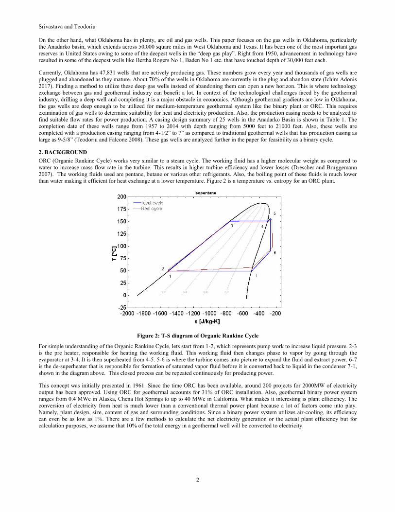
than water making it efficient for heat exchange at a lower temperature. Figure 2 is a temperature vs. entropy for an ORC plant.

Figure 2: T-S diagram of Organic Rankine Cycle

For simple understanding of the Organic Rankine Cycle, lets start from 1-2, which represents pump work to increase liquid pressure. 2-3

is the pre heater, responsible for heating the working fluid. This working fluid then changes phase to vapor by going through the

evaporator at 3-4. It is then superheated from 4-5. 5-6 is where the turbine comes into picture to expand the fluid and extract power. 6-7

is the de-superheater that is responsible for formation of saturated vapor fluid before it is converted back to liquid in the condenser 7-1,

shown in the diagram above. This closed process can be repeated continuously for producing power.

This concept was initially presented in 1961. Since the time ORC has been available, around 200 projects for 2000MW of electricity

output has been approved. Using ORC for geothermal accounts for 31% of ORC installation. Also, geothermal binary power system

ranges from 0.4 MWe in Alaska, Chena Hot Springs to up to 40 MWe in California. What makes it interesting is plant efficiency. The

conversion of electricity from heat is much lower than a conventional thermal power plant because a lot of factors come into play.

Namely, plant design, size, content of gas and surrounding conditions. Since a binary power system utilizes air-cooling, its efficiency

can even be as low as 1%. There are a few methods to calculate the net electricity generation or the actual plant efficiency but for

calculation purposes, we assume that 10% of the total energy in a geothermal well will be converted to electricity.

Srivastava and Teodoriu

3

Figure 3: Geothermal Map of Oklahoma (Cheung , 1979)

3. ELECTRICITY GENERATION FROM GAS WELLS

The following part is focusing on the understanding of maximum geothermal production from gas wells. Our focus is on those wells that

are at the latest phase of their production, considering a smooth transition from gas to power to heat to power concept.

3.1 Estimating Temperature Gradients

Oklahoma lies in a moderate thermal gradient. OGS (Oklahoma Geological Survey) recognizes an average gradient of 1.3°F/100ft as

shown in Figure 3 below. Using this gradient, the temperature at the bottom of the wells can be calculated for our 25 wells in study. The

surface temperature is assumed as 40°F for calculations. Figure 4 shows the geothermal gradient for Oklahoma as compared to a higher

gradient of 2.5°F/100ft. Some of the deepest wells in Oklahoma ranging in depths of 20,000 ft. have a temperature of only 150°C as

seen in Figure 4. This makes binary power cycle as the only viable option in Oklahoma. In comparison, conventional geothermal

systems have gradients that lie in the range of 2.5-3°F/100ft and therefore have a temperature of 275 C at the same depth of 20000 ft.

Srivastava and Teodoriu

4

Figure 4: Geothermal gradient comparison

3.2 Flow Rates And Flow Velocities

We assume that pure water is used for circulation in the thermal cycle. This assumption helps in ruling out inconsistencies in fluid

properties like density and heat capacity if brine were to be considered, due to high salt content. Moreover, pure water has a higher

thermal capacity and is easier for calculation purposes. A heat capacity value of 4183 J / kgK is used for calculation of thermal power

output as seen in section 2.4. The flow rates can be calculated as a product of the flow velocity of fluid and the cross sectional area.

Ideally, a power plant system has an installed capacity value for which it is designed. The required flow rates of the fluids used in the

cycle are calculated as per the power output. Even the well is designed as per the requirement of a range of flow velocities or flow rates.

In our case we have a pre-existing design of the well that is already available for us to utilize. Conventional geothermal systems have

flow rates not higher than 120 l/s as pressure drop starts to increase dramatically due to friction (Iska and Teodoriu, 2010). These

pressure losses are even higher in smaller diameter pipes. Gas wells in Oklahoma as studied in Table 1 have smaller casing sizes at

producing depth. We therefore opted to analyze different flow rates for the range of production casing designs in Oklahoma wells to

determine an optimum flow rate for water keeping pressure losses in mind. The pressure losses were determined and thus a viable power

output could be determined for the wells. The production casing sizes that are analyzed range from 4-1/2” to 9-5/8”. The flow rates vary

from 30 l/s to 70 l/s. Figure 5 shows the calculated flow velocities in m/s for various casing sizes. The highest velocity being 8.26 m/s

for 4-1/2” casing at 70l/s flow rate. N80 and P110 are commonly used steel grades for production casing in gas wells under study. The

IDs of the casing used are standard ID values for N80 grade.

Figure 5: Flow velocities in m/s at different flow rates

3.3 Pressure Losses

For pressure loss calculations, a straight pipe with circular cross section is considered. An average length of 10,000 ft. is considered for

calculation purposes. There are a lot of factors that influence pressure losses in a pipe such as flow velocity, dimensions of the wetting

surface, type of flow, fluid properties and finally surface roughness of the wall in contact with the fluid. Since we use water, which is an

incompressible fluid, Darcy-Weisbach equation can be used to calculate pressure drop due to friction along the length of pipe. Pressure

loss is defined as,

∆𝑃 = 𝑓𝐷. 𝐿.𝜌

2

𝑣2

𝐷

Srivastava and Teodoriu

5

where ΔP, ƒD, L, v, D are pressure loss, Darcy friction factor , length of pipe, flow velocity and diameter respectively. ƒD is also called the flow co-efficient and is calculated using Moody’s chart or through Colebrook equation, which is an implicit equation and therefore needs iteration. Swamee Jain, 1976, approximates Colebrook-White equation to help calculate Darcy friction factor. The equation is dependent on wall roughness and Reynolds number of the flowing fluid.

𝑓𝐷 = 0.25 [log ( 𝑒

𝐷⁄

3.7+

5.74

𝑅𝑒0.9)

]

−2

where e , D, Re are wall roughness, diameter of pipe and Reynolds number respectively. The surface is assumed as steel with a roughness of 0.025mm. This assumes a turbulent flow in the pipe. Using these equations, pressure drop is calculated for various production casing sizes at varying flow rates at an average depth of 10000 ft. Figure 6 shows the pressure losses due to friction for various flow rates and inner diameters of the feed pipes.

Figure 6: Pressure drop over different flow rates and casing ID

As seen in Figure 6, some of the pressure values are marked in red and some in green. Pressure values above 40 bar are not economical

for our system. The 40 bar value takes into account pump placement. Since the pump should ideally be placed no deeper than 400-

500m, we calculate the maximum frictional pressure drop that is neutralized by lowering the pump into the well. Since 40 bar of

pressure equals 410 meters of hydrostatic head, our assumption is right. Values lower than 40 bar are ideal for power production using

binary system. Casing sizes 8-5/8” and 9-5/8”, though the right size for a conventional geothermal well, are still marked in red because

the wells being considered are pre-drilled wells and do not have a large production casing diameter. It would be uneconomical to go for

a re-completion job on these wells again. The pressure losses are also plotted in Figure 7. The highest frictional pressure loss is observed

in 4-1/2” casing at 70 l/s. The flow velocity was also maximum in this case as seen in the previous section. Frictional pressure losses

increase with higher flow rates and decrease with increasing casing diameters. Thus finding an optimum value for electricity production

is crucial.

Figure 7: Pressure loss variation with Flow rate and Casing ID

Srivastava and Teodoriu

6

3.4 Electric Output

As discussed earlier, the electric power output is a fraction of the thermal power output of the system. In the case of ORC binary power

system, we assumed an efficiency of 10 %. Thermal power output of the system is defined below.

𝑃𝑡ℎ = �̇�𝑐𝑝∆𝑇

Simplifying,

𝑃𝑡ℎ = 𝜌�̇�𝑐𝑝∆𝑇

where ρ, 𝑐𝑝, �̇�, �̇� is the density, specific heat capacity, mass flow rate and volumetric flow rate of water. ∆𝑇 is the temperature

difference between the production and injection line. The injection temperature is taken as 70 C in our calculations. Using the equations

mentioned above, the thermal power output can be easily calculated. Figure 8 displays the electric power output for 3 various

temperature difference cases of 20, 40 and 60° C. As mentioned in our abstract, we aimed at producing 500kW of electric power output

from each gas well. We also defined efficiency η to produce electricity from thermal power at 10% for our case. In such a case;

𝑃𝑒𝑙 = 𝑃𝑡ℎ 𝑋 𝜂

where 𝑃𝑒𝑙, 𝑃𝑡ℎ are the electric and thermal power output respectively. If one closely observes the graph below, 500 kW can be produced

in all three cases of temperature differences with more freedom of choosing flow rates for 20 C difference in temperature. Since 5-1/2”

production casing has been most commonly used in our study, we look closely at power outputs and pressure drops for the same. A

quick recap from Figure 6 shows that up to 60 l/s can be used in 5-1/2” and the pressure drop will still remain below 40 bar.

Figure 8: Electric power calculated for ΔT of 20, 40, 60 C

Figure 9 is a focused study on 5-1/2” casing. The electric power output remains the same for various temperature differences but the

graph has an additional plot of pumping power, which is a function of flow rate and pressure loss. As one can observe for 5-1/2” casing,

temperature differences of 20, 40 and 60 can all work economically to produce 500kW of electric output but with varying pressure

losses. Although working with temperature difference of 20 C seems more feasible as it would require a low-temperature resource,

power lost to pumping is high. On the other hand, lower flow rates but higher temperature difference is a more preferable option. Lets

take the maximum and minimum flow rates to find the power lost to pumping for same power output of 500kW. Pressure loss for 30

and 50 l/s flow rate are 10.31 and 52.41 bar. The pumping power thus calculated is 30.9kW and 262 kW respectively as seen in figure 9.

Srivastava and Teodoriu

7

Figure 9: Electric and pump power vs. pressure loss for 5-1/2”

Figure 10 summarizes the power utilization for 5-1/2” casing. Clearly using a temperature difference of 20 C and a high flow rate of 70

l/s is not feasible as more than 50% of the expected power output is utilized in pumping as compared to only 6% in the case of 60 C

temperature difference and flow rate of 30 l/s.

Figure 10: Breakdown of power utilization for 5-1/2” casing

Considering the high number of abandoned gas wells, we propose the use of the wellhead-produced electricity for energy compensation.

For example, the grid power when other renewable do not provide the required amount. Moreover, considering that the number of wells

being abandoned are high, 100 wells will deliver 50 MW. The gas production that will take place in the last phase of gas depletion (we

estimate at least 2 to 5% recoverable gas in place) through the water circulation for geothermal production to be extracted will bring the

gas recovery factor to almost 100%. This gas could be used either to increase the input water temperature or to cogenerate heat and

electricity through use of a microtrubine. This combination may lower the time to recover the investment and accelerate the heat to

power the wellhead concept.

Srivastava and Teodoriu

8

4. CONCLUSIONS

The paper is investigating an alternative concept to implement low enthalpy geothermal in Oklahoma, which is known to have no

geothermal production as of today. The study has analyzed the utilization of deep gas wells, some having the potential of providing a

temperature source of up to 150°C.

The study shows that the gas wells in Oklahoma have production casing sizes from 4 1/2" to 7", thus optimizing gas wells as a

geothermal resource can be done. Our calculations have shown that some wells, at flow rates of 30 l/s can produce sufficient heat to

generate about 500kW using an ORC generator. At 30 l/s, the lowest size of the production casing is 4 1/2" although a 5" is more

appropriate. After carefully analyzing thermal and electric power outputs using binary cycle and calculating power losses in pumping,

we conclude that larger the production casing ID, the smaller is the pump power investments, resulting in only 6% of total electric

power production as seen in the case of 5-1/2” production casing.

REFERENCES

U.S Energy Information Administration, Nov 2011. U.S. has large geothermal resources, but recent growth is slower than wind or solar

https://www.eia.gov/todayinenergy/detail.php?id=3970

U.S Energy Information Administration, July 2013. EIA projects world energy consumption will increase 56% by 2040.

https://www.eia.gov/todayinenergy/detail.php?id=12251

Moon Hyungsul, ZarroukSadiq. Efficiency of geothermal power plants: a worldwide review. Department of Engineering Science,

University of Auckland, New Zealand

U.S Energy Information Administration. Number of producing gas wells. https://www.eia.gov/dnav/ng/ng_prod_wells_s1_a.htm

Okech, R. R., Liu, X., Falcone, G., & Teodoriu, C. (2015, November 18). Unconventional Completion Design for Deep Geothermal

Wells. Society of Petroleum Engineers. doi:10.2118/177228-MS

Iska, G. and Teodoriu, C., (2011) An optimization concept for well placement in Enhanced Geothermal Systems based on fracturing

reservoir response, Celle Drilling Conference/gebo, 2011

Hirschfeldt. M. API Casing Table Specification. http://oilproduction.net/files/002-apicasing.pdf

U. Drescher, D. Bruggemann, Fluid selection for the organic Rankine cycle (ORC) in biomass power and heat plants, Applied Thermal

Engineering 2007; 27: 223–228.

Cheung, P.K., 1978. The geothermal gradient in sedimentary rocks in Oklahoma :Oklahoma state university master’s thesis, 55p

Swamee, P., Jain, A., Explicit equations for pipe-flow problems. Journal of the Hydraulics Division (ASCE), 102 (5), 1976, pp. 657–

664.

Ichim Adonis, 2017. Experimental Determination Of Oilfield Cement Properties And Their Influence On Well Integrity. University of

Oklahoma master’s thesis.

Wells A. Bruce, 2018. Anadarko Basin in Depth. https://aoghs.org/editors-picks/anadarko-basin-depth/

Oklahoma Corporation Commission. Oil and Gas info. https://apps.occeweb.com/RBDMSWeb_OK/

Rowshanzadeh Reza. Performance and cost evaluation of Organic Rankine Cycle at different technologies. Department Of Energy

Technology. KTH Sweden.

Srivastava and Teodoriu

9

County Completion Date Status at

completion MD TVD Production Casing

Feet Feet Size Grade Depth TOC

Beaver Nov-87 Flowing 7400 N/A 5-1/2" K55 6756 5980

Beaver Dec-03 Flowing 8100 8019 5-1/2" J55 8084 6180

Beckham Nov-08 Pumping 5150 5150 7 N80 5150 3550

Beckham Oct-01 Flowing 10050 10050 5-1/2" N80 9598 8560

Beckham Sep-08 Flowing 12500 9523 7" P110 9419 6719

Beckham Jan-09 Flowing 11157 6005 5-1/2" N80 11157 3200

Beckham Mar-09 Flowing 10125 N/A 7" N80 10125 9350

Beckham Jul-07 Flowing 12500 9667 7" P110 8880 6380

Beckham Feb-09 Flowing 12100 6313 4-1/2" P110 10965 5880

Beckham Jan-08 N/A 14500 12928 7-5/8" P110 13200 9300

Major Aug-02 Pumping 6848 6669 5-1/2" J55 6735 5374

Major Oct-13 Pumping 8200 8200 5-1/2" NA 8200 5620

Major Feb-88 Flowing 9850 N/A 4-1/2" N80 9850 6900

Major Nov-57 Flowing 9357 N/A 5-1/2" H40 6347 5245

Atoka Jun-08 Flowing 14862 11560 5-1/2" P110 14831 10311

Alfafa Jun-72 Pumping 7505 7505 5-1/2" J55 7302 5650

Custer Aug-00 Flowing 13130 N/A 5-1/2" P110 11785 N/A

Woods Feb-08 Flowing 6500 N/A 5-1/2" J55 6500 3960

Woods Jun-98 Flowing 5150 N/A 4-1/2" J55 5150 4320

Blaine Dec-11 Flowing 19705 15099 5-1/2" P110 19705 10000

Blaine Nov-14 Flowing 16840 12091 5-1/2" P110 16840 8735

Pittsburgh Oct-12 Flowing 17424 12573 5-1/2" P110 17424 8000

Pittsburgh Oct-12 Flowing 16891 12261 5-1/2" P110 16891 10190

Blaine Sep-93 Flowing 8000 NA 4-1/2" J55 8000 6750

Blaine Nov-90 Flowing 8700 NA 4-1/2" J55 8703 6400

Blaine N/A Flowing 20933 16023 5-1/2" P110 20933 12000

Table 1: List of 25 wells of Anadarko basin used for geothermal prospect analysis.