Gas-Liquid Stratified Flow in Pipeline with Phase …fluctuations, and pipeline blockage or...

Chapter 4

Gas-Liquid Stratified Flow in Pipeline with Phase

Change

Guoxi He, Yansong Li, Baoying Wang,Mohan Lin and Yongtu Liang

Additional information is available at the end of the chapter

http://dx.doi.org/10.5772/intechopen.74102

Provisional chapter

Gas-Liquid Stratified Flow in Pipeline with PhaseChange

Guoxi He, Yansong Li, Baoying Wang,Mohan Lin and Yongtu Liang

Additional information is available at the end of the chapter

Abstract

When the natural gas with vapor is flowing in production pipeline, condensation occursand leads to serious problems such as condensed liquid accumulation, pressure and flowrate fluctuations, and pipeline blockage. This chapter aims at studying phase change ofvapor and liquid-level change during the condensing process of water-bearing natural gascharacterized by coupled hydrothermal transition and phase change process. A hydro-thermal mass transfer coupling model is established. The bipolar coordinate system isutilized to obtain a rectangular calculation domain. An adaptive meshing method isdeveloped to automatically refine the grid near the gas-liquid interface. During phasechange process, the temperature drop along the pipe leads to the reduction of gas massflow rate and the rise of liquid level, which results in further pressure drop. Latent heat isreleased during the vapor condensing process which slows down the temperature drop.Larger temperature drop results in bigger liquid holdup while larger pressure drop causessmaller liquid holdup. The value of velocity with phase change is smaller than thatwithout phase change while the temperature with phase change is bigger. The highesttemperature locates in gas phase. But near the pipe wall the temperature of liquid region ishigher than gas region.

Keywords: hydrocarbons pipeline, vapor/condensation-stratified flow, heat transfer,phase change, multi-component

1. Introduction

Condensation occurs when the natural gas with vapor is flowing in production pipeline andleads to serious problems such as condensed liquid accumulation, pressure and flow rate

© 2016 The Author(s). Licensee InTech. This chapter is distributed under the terms of the Creative Commons

Attribution License (http://creativecommons.org/licenses/by/3.0), which permits unrestricted use,

distribution, and eproduction in any medium, provided the original work is properly cited.

DOI: 10.5772/intechopen.74102

© 2018 The Author(s). Licensee IntechOpen. This chapter is distributed under the terms of the CreativeCommons Attribution License (http://creativecommons.org/licenses/by/3.0), which permits unrestricted use,distribution, and reproduction in any medium, provided the original work is properly cited.

fluctuations, and pipeline blockage or corrosion. The pipe flow together with phase change iscommonly encountered in various heat and mass transfer processes over the past four decades,for instance, in petroleum and chemical processing industry, steam-generating equipment,nuclear reactors, geothermal fields, heat exchangers, cooling systems, and solar energy system[1–4]. In petroleum transportation, two-phase flow characterization is a very common andeconomic technique, where vapor-liquid two-phase stratified flow is often observed in hori-zontal or slightly inclined systems [5, 6].

There exist several problems in the pipeline network system that the saturated vapor in gaswould condense due to pressure and temperature drop [7, 8]. The condensate would attach tothe pipe wall as a form of film or droplet [9, 10]. The condensation will decrease the effectivecross-sectional area and cause the increase of pressure drop which may lead to system shut-down [11, 16]. Generally, the condensed water accumulates at the lower parts of the pipelinedue to the hilly pipeline route topography, which results in a continuous change of liquidholdup along the pipeline [12–14]. The changing liquid holdup and flow area are bounded toaffect the flow patterns which inevitably influence the operating pressure and temperatureinversely. Thus, the flow of condensed water and water-bearing gas in production pipelines isa complex process with coupling of hydraulic, thermal, and phase change phenomena [14–17].Researchers have investigated the gas-liquid two-phase pipe flow system by experiments orhydrodynamic and thermodynamic models.

It has been observed experimentally that when phase change occurs during the saturatedvapor pipeline transportation process, the thermal gradients are created in the wall of thepipeline that lead to severe liquid condensation and stratified vapor-liquid two-phase flow[17, 18]. The fundamental engineering parameters are the pressure drop, liquid holdup, phasefraction, phase flow rate, temperature, thermo-physical properties of the fluids, and pipelinegeometry [19].

Not limited to hydraulic parameters, more recent attention has turned to non-isothermal flowin a pipe or plane channel where some numerical studies are also found [20–27]. The detailedcharacteristic of heat transfer is taken into consideration in these mentioned models instead ofan average value being represented for the temperature profiles in a pipe [28, 29]. According totheir studies, the wall temperature distribution is different from the assumption of fullydeveloped isothermal state [30]. The energy transfer model has been taken into the flowprogress for the optimization of transportation, estimation of corrosion, or prediction of waxdeposition [31, 32]. Concretely, the two-dimensional (2D) momentum and three-dimensional(3D) energy equations for both phases have been established for dynamic and thermal numer-ical simulation [8, 27, 30, 33]. The smooth or wavy interface between phases was obtained in adifferent range of flow rates [17]. For such a two-phase non-isothermal stratified flow, analyt-ical and numerical heat transfer solutions limited to laminar flow and without phase changehave been obtained for fully developed stratified flow under different thermal boundaryconditions [27]. Then, solutions which are more applicable to fully developed turbulent gas-liquid smooth stratified flow have been obtained through the use of high Reynolds model [30].Recently, the steady-state axial momentum and energy equations coupled with a low Reynoldsmodel were established and solved [34]. The pressure drop, liquid height, and temperaturefield which are included in the solutions could match well with the experimental data.

Heat Transfer - Models, Methods and Applications66

However, although equation of state (EOS) was utilized in previous one-dimensional (1D)models to calculate the phase fraction [10, 12, 16, 22, 34, 41, 44], the flow rate, temperature,and pressure were not coupled with the varying liquid level.

According to the description of the physical process of gas-liquid two-phase pipe flow, themodel can be divided into isothermal model, gas-liquid two-phase pipe flow model coupledwith heat and gas-liquid two-phase pipe flow model coupled with heat and mass transfer. Inthe gas-liquid two-phase pipe flowmodel under the isothermal condition, it is assumed that allphases are in thermodynamic equilibrium state without considering the heat transfer processbetween pipe flow and environment, and the physical parameters of gas-liquid two-phase arejust the single value function of pressure. In the gas-liquid two-phase flow model coupled withheat, the heat transfer of gas-liquid and surrounding environment is considered. In the gas-liquid two-phase flow model coupled with heat and mass transfer, the coupling effect of flow,heat transfer, and mass transfer are considered simultaneously.

The two-dimensional (2D) or three-dimensional (3D) stratified gas-liquid two-phase modelincluding mass conversation equation, momentum conversation equation, turbulence modelequation, boundary conditions, and related auxiliary equations for model closure were appliedto describe the flow in pipelines. Differences among them mainly existed in two aspects. Onthe one hand, different turbulence models were built including Spalart-Allmaras Model(SAM), k� εseries model, Reynolds Stress Model (RSM), Direct Numerical Simulation (DNS),and so on. On the other hand, different gas-liquid interface configuration models were builtincluding volume of fluid (VOF) method lattice Boltzmann method, level set method, smoothinterface model, wavy interface model, and curve interface model. The relationship betweenpressure drop, liquid holdup, velocity distribution, turbulent viscosity, and shear stress hasbeen determined through these formula or methods. The flow pattern and flow regime andeven secondary flow have also been discussed under different boundary conditions. However,the energy conservation equation and phase change of fluid components were not taken intoconsideration in those studies.

Recently, attempts have been made to introduce energy equation into the improved modeland the detailed solutions about temperature distribution have also been worked out byconsidering potential energy, kinetic energy, heat transfer, and Joule-Thomson effect [17, 35–38]. The phase change was ignored in these models. Although equation of state (EOS) wasutilized in previous studies to calculate gas condensation of gas-condensate flow in pipelines[12–15, 17–20, 39], the flow rate, temperature, pressure were not coupled with liquid level.Turbulent flow is not considered, which would lead to different numerical results in their one-dimensional (1D) model. Moreover, 1D model could not present the detailed distribution ofhydraulic and thermal parameters at pipe cross-section.

This chapter mainly introduces the different turbulence models, the interface shape model, andthe phase transition model in the process of gas-liquid two-phase stratified flow in the horizontalpipeline. The turbulence model mainly includes the k� ε model, the large eddy simulation (LES)model, and the turbulence model under the low Reynolds number condition at the near wallsurface. The interface shape mainly includes the flat interface model, the wavy interface model,the curve interface model, and the wavy-curve interface model. As a result of the phase transition,a varying wavy curve interface will be produced. If the phase transition is large, the varying wavy

Gas-Liquid Stratified Flow in Pipeline with Phase Changehttp://dx.doi.org/10.5772/intechopen.74102

67

curve interface may gradually become varying wavy flat interface, and finally lead to the changeof flow pattern, no longer the stratified gas-liquid two-phase flow. The phase transformationmodel mainly includes the empirical formula of water vapor phase transformation, the Peng-Robinson (PR) equation of hydrocarbon mixture, the SRK equation, and the PT flash model ofwater hydrocarbon impurities. Also, this chapter compares the different research model, enrichesthe contents of the book, demonstrates the development process of different mathematical modelsin different research points, and finally introduces the development direction of each point in thefuture and the relationship between the complex model and research points.

2. Numerical modeling of stratified gas-liquid wavy pipe flow with phasechange

Since pressure and temperature drop along the pipeline, the saturated vapor of hydrocarbonswould condenses gradually, as shown in Figure 1. The condensed liquid would attach to thepipe wall as liquid film or accumulate at the lower part of the pipeline, which could result incontinuous change of the liquid level [17, 29, 30].

Thus, some models of stratified vapor-liquid two-phase flow coupled with phase change wereproposed. Assumptions could be made as follows: (1) precipitation of condensed liquid is a flashevaporation equilibrium process which occurs in a short moment; (2) regardless of the attach-ment to inner wall of the pipe, all the condensed liquid accumulates at the bottom of the pipe;(3) two-phase flow in vapor-liquid pipeline has a stratified flow pattern as well as a stabledeveloping flow area in every calculated pipeline segment; (4) the smooth vapor-liquid interfacemodel is adopted to describe the interface shape; (5) the heavy components of hydrocarbon aresimplified as pseudo-componentCþ

7 ; and (6) without considering the effect of gravity on the P–Tflash process.

Several kinds of flow patterns are likely to form for vapor/condensation flowing in pipeline:stratified flow, slug flow, annular flow, and stratified-dispersed flow. It is hard to calculate theliquid level, the exact position of liquid film, and the migration patterns of condensed liquid(as shown in Figure 1) via one-dimensional model which could not present the detailed

Figure 1. Vapor-liquid two-phase flow coupled with heat and mass transfer.


distribution of hydraulic and thermal parameters at pipe cross section. Moreover, the 1Dmodel does not consider the turbulent flow which would lead to different numerical results.Hence, the control volume in three-dimensional coordinates is adopted to discretize the calcu-lating area, as shown in Figure 2.

In this section, the governing equations based on physical conservation are chosen andestablished in three-dimensional coordinates, which include mass conservation equation,momentum conservation equation, energy conservation equation, turbulent flow model, andphase change model.

2.1. Mass conservation equation

The total mass flow rate G is the sum of vapor and liquid mass flow rates and keeps constantduring the flowing process:

GG þ GL � G (1)

The mass transfer rate of phase-change within pipe segment has been taken into considerationdue to the vapor phase gradually condensing or the liquid evaporating during the flowprocess. The change of vapor mass flow rate ΔGG is equal to opposite number of that ofliquid�ΔGL:

ΔGG þ ΔGL ¼ ΔG � 0 (2)

The liquid volume fraction HL, vapor volume fraction HG ¼ 1�HL, pressure, vapor, andliquid velocities as well as temperature are the principal unknowns in the cross-sectional areaalong the pipeline. The derivation of mass conservation equation is presented here based ontwo-fluid approach. The mass conservation equations for each phase within the control vol-ume are given as:

HLrL∂wL

∂zþ rLwL

∂HL

∂zþHLwL

∂rL∂P

��T

∂P∂z

þHLwL∂rL∂TL

��P

∂TL

∂z¼ ΔGL

ApipeΔz(3)

HGrG∂wG

∂zþ rGwG

∂HG

∂zþHGwG

∂rG∂P

��T

∂P∂z

þHGwG∂rG∂TG

��P

∂TG

∂z¼ ΔGG

ApipeΔz(4)

Figure 2. Schematic illustration of stratified vapor–liquid flow with phase change.


69

2.2. Momentum conservation equation

The law of momentum conservation is a universal principle for any flow system thatthe varying rate of momentum is equal to the sum of the forces imposed on the controlvolume. Considering the compressibility of vapor and liquid, the equation of momentum isas follows:

∂ rG,LwG,L� �

∂tþ div rG,LwG,L uG,L

��!� � ¼ � ∂p∂z

þ ∂τxz,G,L∂x

þ ∂τyz,G,L∂y

þ ∂τzz,G,L∂z

þ FG,L (5)

here dp=dz is the pressure gradient in the axial direction, Pa=m. In the condition of steady flowstate, the axial pressure gradient dp=dz in liquid is balanced by the shear stress at wall τWL andinterface τint, respectively, in vapor by τWG and τint.

τxz,G,L ¼ μm,G,L∂uG,L∂z þ ∂wG,L

∂x

� �and τyz,G,L ¼ μm,G,L

∂vG,L∂z þ ∂wG,L

∂y

� �represents viscous stress intro-

duced by molecular viscosity; μmdenotes molecular dynamic viscosity; FG,L ¼ rG,L g sinθ.

According to the theory of CFD, the N-S equation is applicable to any kind of flow. A directcalculation of N-S equation requires a high computer capacity which is not practical in engi-neering. Hence, an item of Reynolds is introduced, and the final momentum equation for vaporand liquid stratified flow is as follows:

∂∂x

Γw,G,L∂wG,L

∂x

� � þ ∂∂y

Γw,G,L∂wG,L

∂y

� � ¼ dp

dz� rG,Lg sinθþ ∂rG,LwG,LwG,L

∂z(6)

where Γw,G,L means effective diffusion coefficient, which is the effective viscosity given as thesum of the molecular and eddy viscosity, Γw,G,L ¼ μm,G,L þ μt,G,L.

2.3. Turbulent flow model

Following a similar approach as Xiao et al. [36] and Reboux et al. [37, 38] for two-phaseturbulent flow, the eddy viscosity is modeled using the large eddy simulation (LES) turbu-lence model based on the assumption of non-isotropic turbulence. Meanwhile, changes aremade to take account of the progressive attenuation of turbulence close to the wall. LESmodel is applicable to the flow with different Reynolds number. The subgrid scale viscosity iswritten as:

μt,G,L ¼ rG,Lf int,W CSDSΔð Þ2 Sj jG,L (7)

The Smagorinsky constant is CS ¼ 0:1� 0:2, while the resolved rate-of-strain tensor is:

Sj jG,L ¼ 2SijSij� �1=2

G,L ¼ ∂wG,L

∂x

� 2

þ ∂wG,L

∂y

� 2" #1=2

(8)

The filter width Δ is defined as Δ ¼ Volð Þ1=3, where Vol is the volume of the computational cell.


Damping functions have been introduced into the expressions of turbulent viscosity. Near awall, a wall-damping function is required to perish the eddy viscosity on the wall.

DS ¼ 1� expdþ

25

� ; dþ ¼ rτint,W

� �0:5dμm

; d ¼ minD2�

ffiffiffiffiffiffiffiffiffiffiffiffiffiffiffiffiffiffiffiffiffiffiffiffiffiffiffiffiffiffiffiffiffiffiffiffiffiffiffiffiffiffix2 þ y�D

2þ hL

� 2s

; dj j0@

1A (9)

f int,W ¼ 1� exp �1:3� 10�4dþ � 3:6� 10�4 dþ� �2 � 1:08� 10�5 dþ

� �3h i(10)

And dþ is the dimensionless distance to pipe wall or vapor-liquid interface. Fulgosi et al. [39]provided an exponential dependence of f int on the dimensionless distance to the interface orpipe wall. Parameter d means the distance to pipe wall or vapor-liquid interface.

The choice of turbulence model is crucial for this sort of study, due to the presence of thesesecondary flows. Nallasamy and Rodi explained that the well-known k� ε model assumesan isotropic eddy viscosity, which makes it unsuitable for problems where the anisotropicnature of the turbulent viscosity is important in the calculation of the flow field. This maybecome significant in stratified gas-liquid flow as the height of the interface approaches thecenter of the pipe, as stressed by Newton and Behnia. FLUENT offers different options whenusing this model. Based on the current flow conditions, the linear pressure-strain model andstandard wall functions were selected. Turbulence model used by different researchers isshown in Table 1.

2.4. Heat transfer model

It is of great significance to study turbulent flow and heat-transfer mechanism due to thefrequent occurrence in many industrial applications, such as heat exchangers, vapor tur-bines, cooling systems, and nuclear reactors [27]. In this study, a quasi-steady state oftemperature profile is calculated where axial thermal conduction is neglected. Since theoperating temperature is influenced by ambient temperature, fluid properties, and hydraulicparameters such as flow rate and liquid level; a heat-transfer model for vapor-liquid flow isestablished.

Energy equation means the increase of energy, which is equal to the result of heat flux enteringthe representative-element volume deducting the work from internal force. Ignoring axial heatconduction and viscous dispersive item, the equation of energy conservation is as follows:

∂∂x

ΓT,G,L∂TG,L

∂x

� � þ ∂∂y

ΓT,G,L∂TG,L

∂y

� � ¼ ∂rG,LcP,G,LwG,LTG,L

∂z(11)

ΓT,G,L means effective diffusion coefficient which is the effective heat transfer coefficient and

defined as, ΓT,G,L ¼ μm,G,LcP,G,LPrm,G,L þ μt,G,LcP,G,L

Prt,G,L .μm,G,LcP,G,L

Prm,G,L andμt,G,LcP,G,L

Prt,G,L are respectively molecular ther-

mal diffusion and eddy diffusion of heat transfer. Prm ¼ cPμmλ is molecular Prandtl number. Prt

is turbulent Prandtl number, which is assumed by Jones and Launder as 0.9 [41]. However,Hishida et al. obtained the conclusion that the value of Prt increases with the distance increaseto pipe wall [42]. Only if dþ > 30, Prt is 0.9. When dþ ¼ 10, the value of Prt rises up to 1.6


71

according to the measurement of circular tube of turbulent heat transfer experiments [33].Another calculation of turbulent Prandtl number is given by Kays and Mansoori based on thedirect numerical simulation [27]:

Prt,G,L ¼ 0:5882þ 0:228μt,G,L

μm,G,L

!� 0:0441

μt,G,L

μm,G,L

!2

1� exp �5:165ð Þ μm,G,L

μt,G,L

! !24

35�1

(12)

2.5. Phase change model

The pressure and temperature drop along pipelines, which incurs the change of ratio of gasmass volume and liquid mass volume. It is prone to evoke P–T flash evaporation in eachcomponent. The mass percentage would change accordingly, influencing the parameters likemolar mass, density, viscosity, heat capacity and thermal conductivity. The vapor enthalpywould change during the process of phase change and dissipate into the vapor or liquid in theform of phase change heat which results in variation of fluid temperature [22, 32, 45].

Cong Guo et al. considered a modification of the original model, in which the rate of conductiveheat through the tube wall due to temperature difference can be calculated [43]. Peneloux et al.proposed the concept of volume translation. They argue that the volume obtained usingSRKEOS is a “pseudo-volume” and proposed a method of calculating the “pseudo volume” [44].Sadegh et al. proposed an equilibrium criterion for the Peng-Robinson equation of state (PREOS)based on the volume translated Peng-Robinson equation of state (VTPREOS) and a translatedfunctional relationship is used based on the theory of Peneloux et al. to discuss the volumetranslation technique [45]. The study of Li Zhang et al. shows that the condensation heat transfercoefficient reduces with the increase of wall subcooling from around 2 to 14�C. With the rise inthe wall subcooling, the heat flux increases, resulting in an increasing rate of steam condensation,which brings forth a thicker condensate film on the tube surface. The thicker condensate filmaround the tube offers a higher thermal resistance to steam condensation and in turn reduces thecondensation heat transfer coefficient [22]. Considering the volume addition of LSI phase due to

Formula name expression

Duan et al. [5] Low Reynolds number model:μt ¼ f μCμk2=ε

∂∂x μm þ μt

σk

� �∂k∂x

� �þ ∂

∂y μm þ μtσk

� �∂k∂y

� �þ Gk � rε ¼ 0

∂∂x μm þ μt

σε

� �∂ε∂x

� �þ ∂

∂y μm þ μtσε

� �∂ε∂y

� �þ C1f 1Gk � C2f 2

εk ¼ 0

C1 ¼ 1:92 C2 ¼ 1:3 Cμ ¼ 0:09σk ¼ 1:0 σε ¼ 1:3

f μ ¼ 1� exp �0:0165Rey� �� 2 � 1þ 20:5

Ret

� �f 1 ¼ 1þ 0:05

f μ

� �3f 2 ¼ 1� exp �Re2t

� �Jiang et al. [40] LES model:

μt,G,L ¼ rG,Lf int,W CSDSΔð Þ2 Sj jG,L

Table 1. Different turbulent models.


the coalescence, Kai Yan et al. used the additional velocity and considered all the conditionswhen some portion of SSI phase can come into LSI phase [46]. Bonizzi proposed a model forcalculating the atomization flux and the bulk concentration based on the recommendation byWilliams et al. and Pan and Hanratty [47–51]. Vinesh et al. showed the physical model, consid-ered for phase change which corresponds to hydrodynamically as well as thermally developingvapor-liquid stratified flow in a plane channel, with heating from the top and cooling from thebottom wall [52] (Table 2).

The equation of state in P–T Flash involves Peng-Robinson (PR) equation, which was proposedby Peng-Robinson in 1976. It can predict the molar volume more accurately than SRK equationand can be applied for polar compounds. Apart from that, the equation is applicable to vaporand liquid at the same time and widely used in the calculation of phase equilibrium.

During the P–T flash calculation process, the required parameters are the component of lighthydrocarbon, gasification rate, density, molar mass, and enthalpy. The relation between inputand output is explained in Figures 3 and 4.

The fluid in the pipe includes Nc sorts of hydrocarbon, i ¼ 1, 2,…, Nc. The total energy keepsconstant during the phase change process. When vaporization occurs, excess heat of vapor

Formula name Expression

Cong Guo et al. [43] The rate of conductive heat through the tube wall:Q2 ¼ Δm Cp,2�2 Tv,2�2 � Tf ,2�2

� �þ hfg �� Cp,2�2m1�1 Tf ,2�2 � Tf ,1�1

� �The temperature of the condensate around circumferential wall:Tf ¼ Tw, in þ 0:31 Tv � Tw, inð Þ

Peneloux et al. [44] The “pseudo-volume” obtained using SRKEOS:vactual ¼ vSRKEOS � cThe definition of “pseudo volume”:

~V ¼ V þPni¼1

cizi

Sadegh et al. [45] The “pseudo partial volume” can be defined as:

~vi ¼ ∂ ~V∂zi

� �T,P, zj

¼ vi þ ci j 6¼ i; i ¼ 1, n

With this definition “pseudo fugacity coefficients” can be defined as:

ln ~ϕ i ¼Ð P0

~v iRT � 1

P

� �dP i ¼ 1, n

Kai Yan et al. [46] The expression of the additional velocity UAdd!

:

UAdd, s! ¼

�α3max U!

3 �Um!� �

s; 0

h i, if

∂α2

∂s> 0

�α3min U3! �Um

! Þs; 0� i

, if∂α2

∂s< 0

�8>><>>:

Williams et al. & Pan and Hanratty [47, 48] The atomization flux:

RA ¼ kAu2G rGrLð Þ1=2σGL

ΓZ � ΓZ,Cð ÞIn which kA ≈ 2:0� 10-6 [8, 9].

Bonizzi et al. [51] The flux of droplet deposition is usually expressed as:RDh i ¼ kDCB

CB ¼ EWLQGS

¼ rLαDαG

Table 2. Different phase change models.


73

phase is absorbed from the liquid phase. When condensation occurs, excess heat is releasedfrom the vapor phase. LH represents the latent heat of vaporization or condensation, which iscalculated by [32]:

LH ¼ EG � EL , when condensation occursEL � EG , when vaporization occurs

�(13)

Therefore, the latent heat may result in the temperature change of the vapor-liquid system. Theenthalpy difference in the process of vaporization or condensation can be obtained by virtue ofP–T flash calculation. The latent heat helps to retard the temperature change. The process canbe calculated as follows:

ðAG,L

rG,LwG,LLHlηlξdηdξ ¼ cP,GGGΔTG þ cP,LGLΔTL (14)

The parameters of flow state and related dimensionless parameters are given by:

GG ¼ðAG

rGwGlηlξdηdξ, GL ¼ðAL

rLwLlηlξdηdξ (15)

The properties of fluids are calculated by:

Figure 3. Input and output of P–T flash calculation.

Figure 4. The illustration of the way to obtain the mole fraction by P–T flash in each grid cell.


e;X;Y; rG; rL; rMIX;MG;ML;MMIX;EG;EL;EMIX� � ¼ PREOS Z;P;Tð Þ (16)

μm,G ¼ μm,G TG; rGð Þ,λG ¼ λG TGð Þ, cP,G ¼ cP,G PG;TG;MGð Þ (17)

μm,L ¼ μm,L PL;TL;ML; rL;Xð Þ,λL ¼ λL rL;TLð Þ, cP,L ¼ cP,L rL;TLð Þ (18)

Both gas and liquid phases are not ideal fluids. Vapor phase is a mixture of multi-component light hydrocarbons. Thus, the property of vapor phase is a combination of theirquality weighting. The PREOS equation is currently acknowledged as the most accurateformula to calculate the density of mixed vapor. If the pressure, temperature, and relativedensity of light hydrocarbon are known, the viscosity can be calculated using experimentalformulas. Both the thermal conductivity and the heat capacity at constant pressure forvapor mixture are related to temperature and pressure, which also can be calculated usingthe experimental formulas. For the liquid phase, the density is calculated by PR EOS.The other physical properties including viscosity, thermal conductivity, and specific heatcapacity are respectively a function of temperature, density, and other critical properties ofcomponents.

The relationship between liquid level hLand liquid circulation areaAL is as follows:

ApipeHL ¼ AL ¼ 14D2arccos 1� 2hL

D

� � 14D2 1� 2hL

D

� ffiffiffiffiffiffiffiffiffiffiffiffiffiffiffiffiffiffiffiffiffiffiffiffiffiffiffiffiffiffiffiffiffi1� 1� 2hL

D

� 2s

(19)

The value ofHLas well as the calculating method differs in each cross section, as depicted inFigure 6.

As shown in Figure 6, the evaporation fraction, density, and molar weight of vapor and liquidphase can be obtained with the known mole fraction of each component since the temperatureand pressure are the same as inlet data in the first cross section. The liquid hold-up can becalculated as follows:

HL ¼ 1

1þ rLMGrGML

e1�eð Þ

(20)

The temperature, pressure, and mole fraction vary in the second and other subsequent crosssection due to the influence of thermal conduction, pressure drop, and phase change but can bederived from the former section. Hence, it requires the calculation of the evaporation fraction,density, and molar weight in each grid cell. The liquid holdup can be calculated as follows:

HL ¼P

jrMIX,jML,jMMIX, jrL, j

Aj 1� ej� �

PjrMIX,jMMIX, j

ML,jrL, j

Aj 1� ej� �þ MG,j

rG,jAjej

h i (21)

Then, the liquid level hL can be obtained by Eq. (19).


75

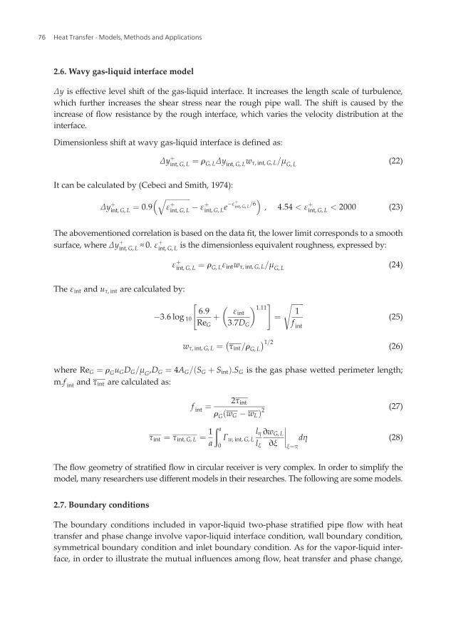
2.6. Wavy gas-liquid interface model

Δy is effective level shift of the gas-liquid interface. It increases the length scale of turbulence,which further increases the shear stress near the rough pipe wall. The shift is caused by theincrease of flow resistance by the rough interface, which varies the velocity distribution at theinterface.

Dimensionless shift at wavy gas-liquid interface is defined as:

Δyþint,G,L ¼ rG,LΔyint,G,Lwτ, int,G,L=μG,L (22)

It can be calculated by (Cebeci and Smith, 1974):

Δyþint,G,L ¼ 0:9ffiffiffiffiffiffiffiffiffiffiffiffiffiffiεþint,G,L

q� εþint,G,Le

�εþint,G,L=6� �

, 4:54 < εþint,G,L < 2000 (23)

The abovementioned correlation is based on the data fit, the lower limit corresponds to a smoothsurface, where Δyþint,G,L ≈ 0. ε

þint,G,L is the dimensionless equivalent roughness, expressed by:

εþint,G,L ¼ rG,Lεintwτ, int,G,L=μG,L (24)

The εint and uτ, int are calculated by:

�3:6 log 106:9ReG

þ εint3:7DG

� 1:11" #

¼ffiffiffiffiffiffiffi1f int

s(25)

wτ, int,G,L ¼ τint=rG,L� �1=2 (26)

where ReG ¼ rGuGDG=μG,DG ¼ 4AG= SG þ Sintð Þ.SG is the gas phase wetted perimeter length;m.f int and τint are calculated as:

f int ¼2τint

rG wG � wLð Þ2 (27)

τint ¼ τint,G,L ¼ 1a

ða0Γw, int,G,L

lηlξ

∂wG,L

∂ξ

��ξ¼π

dη (28)

The flow geometry of stratified flow in circular receiver is very complex. In order to simplify themodel, many researchers use different models in their researches. The following are somemodels.

2.7. Boundary conditions

The boundary conditions included in vapor-liquid two-phase stratified pipe flow with heattransfer and phase change involve vapor-liquid interface condition, wall boundary condition,symmetrical boundary condition and inlet boundary condition. As for the vapor-liquid inter-face, in order to illustrate the mutual influences among flow, heat transfer and phase change,


Formula name expression

Duan et al. [5] ΔEL

¼ 1LΔ EP þ ESð Þ ¼ R3rOilg 1� rGas

rOil

� sin 3θ0

sin 2θ∗ arctanθ∗ � arctanθ0ð Þ π� θ∗ þ 0:5 sin 2θ∗ð Þð Þ þ 23sin 3θP

0

�

þ 2Bo

sinθ0π� θ∗

sinθ∗ � sinθP0 þ cosα θP

0 � θ0� ��

0BBB@

1CCCA

;

Bo ¼ ΔrgR2

σ ;θP0 ¼ cos �1 1� 2hL

R

� �;HL ¼ θP

0� sinθP0

2π ;θ0- sinθ0 cosθ0 ¼ HLπ

Newton and Behnia [20]

The noncircular liquid and gas domains in stratified pipe flow are convenientlymodeled with the bipolar coordinate system described analytically by:

x ¼ c�sinh rð Þcosh rð Þ� cos θð Þ , y ¼ c�sinh θð Þ

cosh rð Þ� cos θð Þ;γ < θ < π, � ∞ < r < þ∞

π < θ < πþ γ, � ∞ < r < þ∞;

where γ is equal to half the angle subtended by the center of the pipe and the gas-liquid interface and is given by:γ ¼ cos -1 1- 2hLD

� �

Badie et al. [53] The apparent rough surface (ARS) model:

εL1-εL ¼

uL,SuG,S

1þ f LrLf irG

� �12

� εL ≤ 0:06f Lf i¼ 108Re�0:726

SL

Badie et al. [53] The double-circle model:PG ¼ π� θð ÞD; PL ¼ θD; Pi ¼ θiDi;

SG ¼ 1� εLð Þ πD2

4 ; SL ¼ εL πD2

4 ;

Di ¼ D sinθsinθi

; θi ¼ sinθsinθi

� �2θþ sin 2θ

tanθi� sin 2θ

2 � πεL� �

Table 3. Different gas-liquid interface models.


77

the equal interfacial shear stress has been prescribed as the vapor-liquid interface conditionwhich is related to the fluid properties and velocity distribution and can be calculated as:

τint,G ¼ μm þ μt

� �G

∂wG

∂n

��int

¼ μm þ μt

� �L

∂wL

∂n

��int

¼ τint, L (29)

The temperature and heat flux of two phases are respectively equal at vapor liquid interface(Table 3).

qint,G ¼ qint,L, Tint,G ¼ Tint, L (30)

At the pipe wall, the non-slip condition is applied for velocity in both two phases.

wW,G,L ¼ 0 (31)

The temperature boundary condition at pipe wall of vapor and liquid phases are convectiveheat transfer and its coefficient of pipeline outer wall remains constant.

αG,L TW � TG,Lð Þ ¼ λG,LdTG,L

dn

��W

(32)

The gradients of velocity and temperature are zero at the symmetrical boundary.

∂wG,L

∂n

��symmetrical

¼ 0,∂TG,L

∂n

��symmetrical

¼ 0 (33)

At the inlet of pipeline, the velocity and temperature filed of two phases are respectively equalto the pipe inlet values.

wG,L ¼ winlet,G,L, TG,L ¼ Tinlet (34)

3. Results and discussion

Based on the theory of flow and heat transfer, turbulent flow and phase equilibrium, the modelis solved by multi-physical field coupling numerical simulation. The non-circular liquid andvapor domains in stratified pipe flow can be simply modeled with the bipolar coordinatesystem, which is helpful in solving the problem caused by the inhomogeneity of boundaries.Bipolar cylindrical coordinate is composed of two orthogonal circles in rectangular coordinate.As the flow field in both phases is bounded by a circular pipe wall and a plane interface, thecalculation domain has been converted to rectangle form from the anomalous physical domainby adopting the bipolar coordinate system.

With the increase of axial distance, the liquid level in pipeline changes constantly and leadsto the change of flow area in both phases. The grid size changes adaptively along withthe flow area, where the flow area is determined by the height of gas-liquid interface.


Variable-size grid has advantages in calculating the changing interface. The grid numberremains unchangeable. The location of the gas-liquid interface is obtained by the secantmethod, and the convergence condition is that the conservation of the mass flow rate of thegas-liquid phase and the total mass flow rate equal to the inlet mass flow rate. In this way,the interface is detected.

Vapor-liquid two phase flow and heat transfer coupled with phase change have been simulatedin this section. The simulated pipeline is with inner diameter of 100 mm and total length of6000 m. The superficial velocities of vapor and liquid are respectively USG ¼ 6:223 m=s andUSL ¼ 0:016 m=s. The pressure gradient is about dp=dz ¼ �21 Pa=m and the liquid holdup atpipe inlet is HL ¼ 0:0343. The mass flow rate of the fluid at pipe inlet is 5.892 kg/s. The fluid ofvapor-liquid mixture at pipe inlet also has a pressure of 10.343 MPa and a temperature of 48�C.The convective heat transfer coefficient is about 10 W= m2 � K� �

and the ambient temperature is15�C. The simulated pipeline is divided into 600 segments where the cross-sectional area of eachsegment has a mesh grid scale of 84� 122 for numerical calculation. The fluid is a mixture ofmulti-component hydrocarbons, which are shown in Table 4.

3.1. Mole fraction, density distribution, and liquid level along the pipeline

The mole fractions of each component, density distribution, temperature distribution, andliquid level along the pipeline are obtained in the condition of condensation production.

Mole fractions of each component at pipe inlet in both phases are shown in Table 5. In vaporphase, the mole fraction of methane is larger than all the other light hydrocarbons (Cþ

2 ). Inliquid phase, the mole fractions of the other light hydrocarbons are bigger than that in vaporphase, but the methane is still the main component.

Mole fractions of each component in both vapor and liquid phase are shown in Figure 5.The content of methane in vapor phase increases when flowing in the pipe while thecontent of the other light hydrocarbons become less and less in vapor phase. During thecondensing process which is dominated by temperature drop, the methane keeps evapo-rating; while during the evaporating process which is dominated by pressure drop, theother light hydrocarbons keep condensing. Meanwhile, the bigger the molar mass is, thefaster the condensing rate is.

Compound CH4 C2H6 C3H8 i-C4H10 n-C4H10 i-C5H12 n-C5H12 n-C6H14 Cþ7

Mole percent (%) 78.03 4.73 5.98 3.05 3.54 2.85 0.54 0.69 0.59

Table 4. Chemical composition of the light hydrocarbons used in current study.

Compound CH4 C2H6 C3H8 i-C4H10 n-C4H10 i-C5H12 n-C5H12 n-C6H14 Cþ7 Total

Mole fraction in vapor phase (%) 80.54 4.69 5.61 2.71 3.05 2.25 0.41 0.44 0.30 100

Mole fraction in liquid phase (%) 43.31 5.35 11.05 7.82 10.30 11.21 2.32 4.10 4.54 100

Table 5. Mole fraction of each component at pipe inlet in both phases.


79

Six pipe cross sections located at every 1000 m along the pipeline are selected to illustrate thechange of density and temperature distribution, as shown in Figures 6 and 7. It is exactlybecause the pressure on the cross section is the same, so the uneven distribution of thetemperature leads to the uneven distribution of the fluid density. In the two phases, the densitydistribution is opposite to the temperature distribution. The high temperature means lowdensity. The temperature value distributed at every single cross section can be ranked in

Figure 5. Mole fraction of each component changes along pipeline. (left) vapor phase; (right) liquid phase.

Figure 6. Density (dimensionless) distribution depicted in 6 pipe cross sections along the pipeline (every 1000 m).

Figure 7. Temperature (K) depicted in 6 pipe cross sections along the pipeline (every 1000 m).


descending order: the interior of liquid phase, most parts in vapor phase, vapor phase near thetop wall. However, the descending rank of density is liquid phase, vapor phase near the topwall, and the interior of vapor phase. Along the pipeline, the temperature in the areareferenced above decreases gradually while the density increases gradually. Therefore, thetemperature of the sequential cross sections tends to be the same and the density distributionwithin the two phases gradually becomes uniform.

Figure 8 illustrates the selected 12 pipe cross sections located at every 500 m along the pipeline,where the varying trend of liquid level are presented in three-dimensional coordinate system.The minimum liquid level is 7.82 mm at pipeline inlet. The liquid level at outlet is about 16.18 mmand keeps declining trend, which can also be found in Figure 9(b).

Figure 8. Liquid level depicted in 12 pipe cross sections along the pipeline (every 500 m).

Figure 9. Pressure gradient, liquid level, fluid mass flow rate, and temperature along the pipeline. (a) pressure gradient,(b) liquid level, (c) mass flow rate, and (d) bulk temperature.


81

3.2. Pressure gradient, liquid level, fluid mass flow rate, and temperature along the pipeline

The pressure gradient, liquid level, fluid mass flow rate, and temperature along the pipelineobtained in the condition of condensation production have been compared with that found inliterature.

When the phase change behavior is considered along pipe flow, the vapor in gas phase starts tocondense to liquid which begins from the pipe inlet due to the significant temperature drop atpipe wall. The pressure drop fit well with the simulated results presented by Sadegh, as shownin Figure 9(a) [16].

During the condensing process, vapor mass flow rate gradually reduces, as shown in Figure 9(c),and the liquid mass flow rate increases due to the constant total mass flow rate. The increase ofliquid mass flow rate leads to further rise of liquid level, as shown in Figure 9(b).

The liquid holdup firstly increases until it reaches a maximum value and then graduallydecreases. The reason behind this is as follows: The increase of liquid holdup results from theliquid precipitation caused by dominant temperature drop. Due to the large differencebetween fluid temperature and ambient temperature, the amount of liquid precipitation isgreater than liquid evaporation. On the contrary, the decrease of liquid holdup is leaded byliquid evaporation due to dominant pressure drop. Being same to liquid holdup, the liquidmass flow rate maintains the same trend, that is, gradually increasing to reach a maximumvalue and then gradually reduced, which is depicted in Figure 9(c). As the total mass flow isconstant, the mass flow rate of the vapor phase decreases first and then increases. Whencompared with the process of evaporation, the precipitation process caused by temperaturedrop is transient and intense, which is related to the temperature difference between the insideand outside of the pipeline and to the convective heat transfer coefficient.

The tendency of temperature drop is similar to that in the existing research [16]. But there alsoexists difference between vapor bulk temperature, liquid bulk temperature, and the total bulktemperature, which cannot be revealed by one-dimensional model. The liquid bulk tempera-ture is always higher than the vapor bulk temperature while the vapor bulk temperature isalmost always equal to the total bulk temperature. Latent heat is revealed during the vaporcondensing process which slows down the temperature drop, as shown in Figure 9(d).

3.3. Velocity and temperature distribution at pipe length of 3000 m

Through solving the model, with phase change happening, it can be obtained that the pressuregradient is 21.29 Pa/m and the liquid level is 16.02 mm when axial distance reaches 3000 m.

Figure 10(a) shows that the velocity of vapor phase slows down while approaching either thepipe wall or the vapor-liquid interface because of the hindering effects and fluid viscosity. Thevelocity of liquid phase keeps increasing from pipe wall to the interface. The maximumvelocity at the pipe cross section occurs within the vapor phase.

In Figure 10(b) shows that the temperatures of both vapor and liquid phase drop whileapproaching the pipe wall because of the lowest ambient temperature and the convective heat


transfer effects. The temperature of liquid phase keeps increasing from pipe wall to theinterface. The maximum temperature at the pipe cross section exists within the liquid phasenear the interface.

Figure 10(c) shows that the temperature at pipe wall of vapor phase is lower than that of liquidphase when convective heat transfer exists due to the smaller heat carried by the vapor phasethan liquid phase. Thus, lower specific heat capacity results in bigger temperature drop at pipewall of vapor phase. The thermal conductivity of the liquid phase is greater than vapor phase,hence, the temperature gradient in liquid phase is smaller than that in vapor phase, and the bulkaverage temperature of the liquid phase is higher than the vapor phase. Heat is transferring from

Figure 10. Velocity and temperature distribution at pipe length of 3000 m. (a) Velocity profile at pipe cross section; (b) temper-ature profile at pipe cross section; (c) velocity profile at vertical centerline; and (d) temperature profile at vertical centerline.


83

liquid phase to vapor phase through the interface, which makes the temperature drop of theliquid phase and reduces the temperature difference between the two phases.

Figure 10(d) reveals the velocity distribution at the centerline of the pipe. By the dragging forceof the interface, the velocity of liquid phase reaches the maximum value at the interface whilethe velocity of vapor phase reaches the maximum value at the location between the interfaceand its bulk center. The liquid phase slows down while approaching the pipe wall because ofthe hindering of the pipe wall and its high viscosity.

4. Conclusion

The vapor-liquid two-phase pipe flow and heat transfer are studied by virtue of numericalsimulation in light hydrocarbon transportation pipeline coupled with hydraulics, thermody-namics, and phase change. A three-dimensional non-isothermal vapor-liquid stratified flowmodel including phase change model in bipolar coordinate system has been established,where LES turbulence model is utilized to simulate the turbulence flow and the wall attenua-tion function is used to describe the inadequacy performance of vapor-liquid interface. Thevapor phase and the liquid phase are both considered to be compressible and the PR equationof state is chosen for the vapor-liquid equilibrium calculation where the multi-componenthydrocarbon flash calculation is used to evaluate the physical properties, gasification rate,and enthalpy departure of the phases. The P–T flash calculation has been applied to predictthe varying liquid level and the multi-component mass fraction in each phase during theprocess of vapor/liquid stratified pipe flow. The axial pressure gradient, liquid holdup, veloc-ity, and temperature fields have been presented. The fluid mass flow rate, mole fraction,density distribution, and liquid level along the pipeline are also given out.

The simulation results indicate that the influence of pressure and temperature on liquidholdup is different. During the light hydrocarbon transportation process in pipeline, thetemperature drop leads to the reduction of vapor mass flow rate and the rise of liquid level aswell as mass flow rate. Larger temperature drop results in bigger liquid holdup while largerpressure drop causes smaller liquid holdup due to the change of physical properties and phaseequilibrium. After the increase of liquid holdup caused by dominant temperature dropreaching the maximum value, then the decrease of liquid holdup maintains its trend till thepipe outlet, which results from liquid evaporation due to dominant pressure drop.

The highest velocity locates in vapor phase while the highest temperature locates in liquidphase. The liquid bulk temperature is always higher than the vapor bulk temperature. Thevapor bulk temperature is almost always equal to the total bulk temperature, which cannot berevealed by one-dimensional model. Latent heat is revealed during the vapor condensingprocess which slows down the temperature drop. The average velocity of liquid is lower thanthat of vapor, but the temperature of liquid is higher than vapor.

When the fluid flows in the pipeline, the content of methane in vapor phase increasesall the time while the content of the other light hydrocarbons (Cþ

2 ) become less and less.


The condensing rates of the other light hydrocarbons have a positive correlation with theirmolar mass. The temperature value distributed at every single cross section can be rankedin descending order: the interior of liquid phase, most parts in vapor phase, vapor phasenear the top wall. However, the descending rank of density is liquid phase, vapor phase nearthe top wall, and the interior of vapor phase. Along the pipeline, the temperature in the areareferenced above decreases gradually while the density increases gradually. Therefore,the temperature of the sequential cross-sections tends to be the same and the density distri-bution within the two phases gradually becomes uniform. As for the varying trend of liquidlevel presented in three-dimensional coordinate system, it has the same trend of the liquidholdup which firstly increases until it reaches a maximum value and then graduallydecreases.

Thus, models in this chapter can be utilized to accurately predict pressure gradient, velocity,temperature field, liquid holdup, fluid physical properties, and mole fraction, which areessential to the determination of pipe size, design of downstream equipment, and guaranteeof flow assurance.

Acknowledgements

This work was supported by the National Natural Science Foundation of China [Grant number51474228]; and the Beijing Scientific Research and Graduate Joint Training Program [Grantnumber ZX20150440].

Author details

Guoxi He*, Yansong Li, Baoying Wang, Mohan Lin and Yongtu Liang

*Address all correspondence to: [email protected]

Beijing Key Laboratory of Urban Oil and Gas Distribution Technology, China University ofPetroleum-Beijing, Beijing, P.R. China

References

[1] Akansu SO. Heat transfers and pressure drops for porous-ring turbulators in a circularpipe. Applied Energy. 2006;83:280-298

[2] Siavashi M, Bahrami HRT, Saffari H. Numerical investigation of flow characteristics, heattransfer and entropy generation of nanofluid flow inside an annular pipe partially orcompletely filled with porous media using two-phase mixture model. Energy. 2015;93:2451-2466


85

[3] Revellin R, Lips S, Khandekar S. Local entropy generation for saturated two-phase flow.Energy. 2009;34(9):1113-1121

[4] Ferreira RB, Falcão DS, Oliveira VB. Numerical simulations of two-phase flow in ananode gas channel of a proton exchange membrane fuel cell. Energy. 2015;82:619-628

[5] Duan J, Liu H, Gong J, Jiao G: Heat transfer for fully developed stratified wavy gas–liquid two-phase flow in a circular cross-section receiver. Solar Energy. 2015;118:338-349

[6] Lun I, Calay RK, Holdo AE. Modeling two-phase flows using CFD. Applied Energy. 1996;53:299-314

[7] Oliemans RVA. Modeling of gas-condensate flow in horizontal and inclined pipes. In:Proc. of the ASME Pipeline Engineering Symposium-ETCE Dallas; 1987

[8] Adewumi MA, Nor-Azlan N, Tian S. Design approach accounts for condensate in gaspipelines. SPE Eastern Regional Meeting, Society of Petroleum Engineers. 1993

[9] Zhou J, Adewumi MA. Transients in gas-condensate natural gas pipelines. Journal ofEnergy Resource Technology. 1998;120:32-40

[10] Schouten JA, Janssen-van Rosmalen R, Michels JPJ. Condensation in gas transmissionpipelines. International Journal of Hydrogen Energy. 2005;30:661-668

[11] Jin T. Network modeling and prediction of retrograde gas behavior in natural gaspipeline systems [thesis]. Doctoral dissertation. The Pennsylvania State University;2013

[12] Deng D, Gong J. Prediction of transient behaviors of gas-condensate twophase flow inpipelines with low liquid loading. In: 2006 International Pipeline Conference. AmericanSociety of Mechanical Engineers; 2006

[13] Vincent PA, Adewumi MA. Engineering design of gas-condensate pipelines with a com-positional hydrodynamic model. SPE Production Engineers. 1990:5381-5386

[14] Mucharam L, Adewumi MA, Watson RW. Study of gas condensation in transmissionpipelines with a hydrodynamic model. SPE Production Engineers. 1990:5236-5242

[15] Sadegh AA, Adewumi MA. Temperature distribution in natural gas/condensate pipelinesusing a hydrodynamic model. SPE Eastern Regional Meeting; Society of Petroleum Engi-neers. 2005

[16] Abbaspour M, Chapman KS, Glasgow LA. Transient modeling of nonisothermal, dis-persed two-phase flow in natural gas pipelines. Applied Mathematical Modelling. 2010;34:495-507

[17] Dukhovnaya Y, Adewumi MA. Simulation of non-isothermal transients in gas/conden-sate pipelines using TVD scheme. Powder Technology. 2000;112:163-171

[18] Almanza R, Lentz A, Jimeenez G. Receiver behavior in direct steam generation withparabolic troughs. Solar Energy. 1997;61:275-278


[19] Newton CH, Behnia M. A numerical model of stratified wavy gas–liquid pipe flow.Chemical Engineering Science. 2001;56:6851-6861

[20] Newton CH, Behnia M. Numerical calculation of turbulent stratified gas–liquid pipeflows. International Journal of Multiphase Flow. 2000;26:327-337

[21] Berthelsen PA, Ytrehus T. Numerical modeling of stratified turbulent two- and three-phase pipe flow with arbitrary shaped interfaces. In: The 5th International Conferenceon Multiphase Flow; 30 May–4 June, 2004; Yokohama, Japan

[22] Zhang L, Yang S, Xu H: Experimental study on condensation heat transfer characteristicsof steam on horizontal twisted elliptical tubes. Applied Energy. 2012;97:881-887

[23] Gada VH, Datta D, Sharm A. Analytical and numerical study for two-phase stratified-flow in a plane channel subjected to different thermal boundary conditions. InternationalJournal of Thermal Science. 2013;71:88-102

[24] Manabe R. A comprehensive mechanic heat transfer model for two-phase flow with highpressure flow pattern validation [thesis]. Department of Petroleum Engineering: Univer-sity of Tulsa; 2001

[25] Fontoura VR, Matos EM, Nunhez JR. A three-dimensional two-phase flow model withphase change inside a tube of petrochemical pre-heaters. Fuel. 2013;110:196-203

[26] Mansoori Z, Yoosefabadi ZT, Saffar-Avval M. Two dimensional hydro dynamic and ther-mal modeling of a turbulent two phase stratified gas–liquid pipe flow. In: ASME 2009Fluids Engineering Division Summer Meeting. American Society of Mechanical Engineers;2009. p. 753-758

[27] Singh AK, Goerke UJ, Kolditz O. Numerical simulation of non-isothermal compositional gasflow: application to carbon dioxide injection into gas reservoirs. Energy. 2011;36:3446-3458

[28] Ebadian MA, Vafai K, Lavine A. Single and multiphase convective heat transfer. AppliedEnergy. 1992;43:291-292

[29] Gong G, Chen F, Su H, Zhou J. Thermodynamic simulation of condensation heat recoverycharacteristics of a single stage centrifugal chiller in a hotel. Applied Energy. 2012;91:326-333

[30] Hu H, Zhang C. A modified k–e turbulence model for the simulation of two-phase flowand heat transfer in condensers. International Journal of Heat and Mass Transfer. 2007;50:1641-1648

[31] Sarica C, Panacharoensawad E. Review of paraffin deposition research under multiphaseflow conditions. Energy Fuel. 2012;26:3968-3978

[32] Duan J, Gong J, Yao H. Numerical modeling for stratified gas–liquid flow and heattransfer in pipeline. Applied Energy. 2014;115:83-94

[33] Ullmann A, Brauner N. Closure relations for two-fluid models for two-phase stratifiedsmooth and stratified wavy flows. International Journal of Multiphase Flow. 2006;32(1):82-105


87

[34] Vincent PA, Adewumi MA. Engineering design of gas-condensate pipelines with a com-positional hydrodynamic model. SPE Production Engineers. 1990;5(04):381-386

[35] Haaland SE. Simple and explicit formulas for the friction factor in turbulent pipe flow.Fluids Engineering. 1983;105:89-90

[36] Helgans B, Richter DH. Turbulent latent and sensible heat flux in the presence of evapo-rative droplets. International Journal of Multiphase Flow. 2016;78:1-11

[37] Vargaftik NB, editor. Handbook of Physical Properties of Liquids and Gases-pure Sub-stances and Mixtures. Hemisphere Pub; 1975

[38] DenHerder T. Design and simulation of PV super system using simulink [thesis]. San LuisObispo: California Polytechnic State University; 2006

[39] Zaghloul JS. Multiphase analysis of three-phase (gas-condensate-water) flow in pipes(Doctoral dissertation [thesis]). Pennsylvania State University; 2006

[40] Jiang X, Siamas GA, Jagus K, et al. Physical modeling and advanced simulations of gas–liquid two-phase jet flows in atomization and sprays. Progress in Energy & CombustionScience. 2010;36(2):131-167

[41] Jones WP, Launder BE. The calculation of low-Reynolds-number phenomena with a two-equation model of turbulence. International Journal of Heat and Mass Transfer. 1973;16(6):1119-1130

[42] Hishida M, Nagano Y, TagawaM. Transport processes of heat and momentum in the wallregion of turbulent pipe flow. In: Proceedings of the 8th International Heat TransferConference. Hemisphere Publishing Corp; 1986;Washington, DC; 1986. p. 925-930

[43] Guo C, Wang T, Hu X, et al. Experimental investigation of the effects of heat transportpipeline configurations on the performance of a passive phase-change cooling system.Experimental Thermal and Fluid Science. 2014;55:21-28

[44] Péneloux A, Rauzy E, Fréze R. A consistent correction for Redlich-Kwong-Soave vol-umes. Fluid Phase Equilibria. 1982;8(1):7-23

[45] Sadegh A A, Adewumi M A. Temperature distribution in natural gas/condensate pipe-lines using a hydrodynamic model. In: SPE Eastern Regional Meeting. Society of Petro-leum Engineers; January, 2005

[46] Yan K, Zhe D. A coupled model for simulation of the gas–liquid two-phase flow withcomplex flow patterns. International Journal of Multiphase Flow. 2010;36(4):333-348

[47] Williams LR, Dykhno LA, Hanratty TJ. Droplet flux distributions and entrainment inhorizontal gas–liquid flows. International journal of multiphase flow. 1996;22(1):1-18

[48] Pan L, Hanratty TJ. Correlation of entrainment for annular flow in horizontal pipes.International Journal of Multiphase Flow. 2002;28(3):385-408


[49] Laurinat JE, Hanratty TJ, Jepson WP. Film thickness distribution for gas–liquid annularflow in a horizontal pipe. PhysicoChemical Hydrodynamics. 1985;6(1):79-195

[50] Pitton E, Ciandri P, Margarone M, Andreussi P: An experimental study of stratified–dispersed flow in horizontal pipes. International Journal of Multiphase Flow. 2014;6:92-103

[51] Bonizzi M, Andreussi P. Prediction of the liquid film distribution in stratified-dispersedgas–liquid flow. Chemical Engineering Science. 2016;142:165-179

[52] Gada VH, Datta D, Sharma A. Analytical and numerical study for two-phase stratified-flow in a plane channel subjected to different thermal boundary conditions. InternationalJournal of Thermal Sciences. 2013;71:88-102

[53] Badie S, Hale CP, Lawrence CJ, et al. Pressure gradient and holdup in horizontal two-phase gas–liquid flows with low liquid loading. International Journal of Multiphase Flow.2000;26(9):1525-1543


89

Gas-Liquid Stratified Flow in Pipeline with Phase …fluctuations, and pipeline blockage or...

Documents

Transcript of Gas-Liquid Stratified Flow in Pipeline with Phase …fluctuations, and pipeline blockage or...