HAL Id: hal-00564549https://hal.archives-ouvertes.fr/hal-00564549

Submitted on 9 Feb 2011

HAL is a multi-disciplinary open accessarchive for the deposit and dissemination of sci-entific research documents, whether they are pub-lished or not. The documents may come fromteaching and research institutions in France orabroad, or from public or private research centers.

L’archive ouverte pluridisciplinaire HAL, estdestinée au dépôt et à la diffusion de documentsscientifiques de niveau recherche, publiés ou non,émanant des établissements d’enseignement et derecherche français ou étrangers, des laboratoirespublics ou privés.

Gas hydrate equilibria for CO2–N2 and CO2–CH4 gasmixtures-Experimental studies and thermodynamic

modellingJean-Michel Herri, Amina Bouchemoua-Benaissa, Matthias Kwaterski, Amara

Fezoua, Yamina Ouabbas, Ana Cameirão

To cite this version:Jean-Michel Herri, Amina Bouchemoua-Benaissa, Matthias Kwaterski, Amara Fezoua, Yamina Ouab-bas, et al.. Gas hydrate equilibria for CO2–N2 and CO2–CH4 gas mixtures-Experimental stud-ies and thermodynamic modelling. Fluid Phase Equilibria, Elsevier, 2011, 301 (2), pp.171-190.�10.1016/j.fluid.2010.09.041�. �hal-00564549�

Gas Hydrate Equilibria for CO2-N2 and CO2-CH4 gas mixtures

– Experimental studies and Thermodynamic Modelling

Herri J.-M. ∗ , Bouchemoua A., Kwaterski , M., Fezoua A., Ouabbas Y., Cameirao A.

Ecole Nationale Supérieure des Mines de St-Etienne 158 cours Fauriel,

42023 St-Etienne, FRANCE

Abstract

In this paper, a set of experimental data on the phase equilibrium of gas hydrates in the

presence of binary gas mixtures comprising CO2 is presented. The procedure established

allows for the determination of both the composition of the gas phase as well as the hydrate

phase without the need to sample the hydrate. The experimental results obtained in these

measurements have been described by means of the classical model of van der Waals and

Platteeuw. The values of internal parameters of the reference state and the Kihara parameters

have been re-discussed and their interdependency is pointed. Finally the new set of parameters

is validated against experimental data from other sources available in the literature, or

invalidated against other sources. Finally, we conclude on the difference of experimental data

between laboratories. The differences are not on the classical (Pressure, Temperature, gas

composition) data which appear equivalent between laboratories. The difference stands on the

measurement composition of the hydrate phase.

Keywords: gas hydrates, thermodynamic, crystallization, modeling

∗ Corresponding author: Phone: +33 4 77 42 02 92 Fax +33 4 77 49 96 94 E-mail: herri@emse.fr

1

1 Introduction

CO2 capture in industry is a challenge that is suitable for reducing the global carbon

emissions. The gases emitted by industry are by definition localized at the plants, like e.g.

steelmaking plants, gas or coal power plants, chemical plants or natural gas production plants.

For that reason it is envisaged to employ industrial process to remove those industrial gases

that have an impact on the global warming before being emitted into the atmosphere.

However, in designing processes for removal of these green house gases, it is very important

to consider the quantities to be treated. In case of steelmaking plants for example, the

emissions can be in the order of several cubic meters per second of CO2. In power plants, the

concentration of CO2 is generally low, typically in the range of 5-15%, but it can be several

tens of percents in steelmaking plants or in some cases of natural gas production.

Facing the variety of gases to be treated with regard to their quantities, qualities (mainly the

CO2 content, but also the presence of minor impurities such as H2S, SO2, NOX….), and

conditions of pressure and temperature, different strategies and technologies need to be

developed to minimize the cost of the process.

Hydrate technology could be an alternative approach to remove green house gases and this is

the route we try to develop. A preliminary costing has revealed the process to be competitive

for high concentrated mixtures of CO2 containing N2 (Nuyeng et al, 2007) such as found in

exhaust gases of steel making plants at atmospheric pressure.

Currently we are working on the accurate modeling of hydrate equilibria in the presence of

multiple gas components. The respective routines are to be implemented into process

simulation software allowing for the precise evaluation of different sizing and costing

schemes of capture. This work presents a set of experimental data on the CO2-N2 and CO2-

CH4 hydrate equilibria with pure water. We present in detail our experimental procedure by

2

which the gas composition can be measured directly, whereas the hydrate composition is to be

calculated from a mass balance.

Furthermore we have tried to validate our experimental data by using the classical van der

Waals and Platteeuw model (1959) with internal parameters found in the literature. These

parameters are the so-called macroscopic parameters (i.e. macroscopic parameters from Table

3 which refer to a classical thermodynamic approach) and the so-called Kihara parameters

(referring to a statistical approach).

Due to large deviations between the modeled values obtained in the way described above and

the experimental results, we have re-fitted the internal parameters, essentially by retaining a

set of macroscopic parameters from Handa and Tse (1986), and re-fitting the Kihara

parameters from our experimental results. Finally the new set of parameters is validated

against experimental data from other sources available in the literature, or invalidated against

other sources.

2 Gas Hydrates

The clathrates are ice-like compounds in the sense that they correspond to a re-organisation of

the water molecules to form a solid. The crystallographic structure is based on H-bonds. The

clathrates of water are also designated improperly as “porous ice” because the water

molecules build a solid network of cavities in which gases, volatile liquids or other small

molecules could be captured.

The clathrates of gases, called gas hydrates, have been studied intensively due to their

occurrence in deep sea pipelines where they cause serious problems of flow assurance.

Each structure is a combination of different types of polyhedra sharing faces between them.

Jeffrey (1984) suggested the nomenclature ef to describe each polyhedra: e is the number of

edges of the face, and f is the number of faces with e edges. Currently, three different

3

structures have been established precisely, called I, II and H (Sloan, 1998, Sloan and Koh,

2007)

Table 1 Structure of gas hydrates SI SII SH

Cavity 512 51262 512 51264 512 435663 51268

Type of cavity (j: indexing number)

1 2 1 3 1 5 4

Number of cavities (mj) 2 6 16 8 3 2 1 Average cavity radius

(nm)(1) 0.395 0.433 0.391 0.473 0.391 0.406 0.571

Variation in radius, % (2) 3.4 14.4 5.5 1.73 Coordination number 20 24 20 28 20 20 36

Number of water molecules 42 136 134 Cell parameters (nm) a= 1.1956 (3) a=1.7315 (4) a=1.2217, b=1.0053 (5) Cell volume (nm3) 1.709 (3) 5.192 (4) 1.22994 (5) (1) Sloan (1998, p. 33). (2) Variation in distance of oxygen atoms from centre of cages (Sloan, 1998, p. 33). (3) For ethane hydrate, from (Udachin, 2002). (4) For tetrahydrofuran hydrate, from Udachin (2002). (5) For methylcyclohexane-methane hydrate, from Udachin (2002).

3 Experimetal procedure and set-up

3.1 Experimental set-up

An experimental apparatus (Fig. 1) has been built to investigate the thermodynamic

equilibrium conditions of gas hydrates (pressure and temperature) and to determine the

composition of all existing phases (gas, liquid and hydrate). The experimental set-up consists

of a stainless steel high pressure batch reactor (Autoclave) with a double jacket connected to

an external cooler (HUBERT CC-505) with a CC3 controller maintaining the temperature

with a precision of 0.02 K. Two sapphire windows of (12 x 2 cm) mounted on both sides of

the reactor enable to detect the occurrence of a hydrate phase by direct visual observation. A

Pyrex cell is located in the stainless steel autoclave in which the pressure can be raised up to

4

10 MPa. The Pyrex cylinder is filled with 800 ml to 1 l of water containing LiNO3 as an

anionic tracer at a concentration of approximately 10 to 15 ppm (weight). The liquid is

injected in the pressurized reactor by using a HPLC pump (JASCO-PU-1587). A four

vertical-blade turbine impeller ensures stirring of the suspension during crystallization. The

temperature is monitored by two Pt100 probes, one in the liquid bulk, and the other one in the

gas phase (Prosensor instrument, precision of 0.02 K). The pressure is measured by mean of a

pressure transducer (range: 0–10 MPa (Keller instrument, precision of 0.05 MPa). The data

acquisition unit (T, P) is connected to a personal computer. The composition of the gas phase

is determined in line by using a gas chromatograph after sampling by a ROLSI instrument.

This tool collects a controlled volume of gas (some μm3) which is directly injected into the

loop of the gas chromatograph (VARIAN model CP-3800 GC). The precision in gas

composition is 2% (see annex 1)

A classical valve is used to take a sample of 1 ml of liquid which is directed to a DIONEX

ionic exchange chromatograph (off-line) to measure the tracer (LiNO3) concentration. The

tracer is an ionic element which is not incorporated into the hydrate structure but concentrated

in the liquid phase during crystallization.

The gas mixtures are prepared by injecting each gas directly into the reactor. The mixtures are

analyzed by gas chromatography to obtain the exact composition of each gas (see annex 1)

5

Fig. 1 Experimental setup

3.2 Experimental procedure

The hydrate is obtained by crystallization of gas mixtures (CO2 with N2 or CH4) in presence of

a liquid phase (water + LiNO3 (10 ppm weight fraction)).

Initially the reactor is closed and evacuated by means of a vacuum pump. Subsequently, the

cell is flushed three times with nitrogen (or CH4, depending on the experiment) to eliminate

any trace of other gases (e.g. from a preceding experimental run). After this cleaning

procedure, the reactor is evacuated again.

At the beginning of the actual experimental run, the reactor is pressurized with the first gas

(generally this has been CO2 because the maximum pressure in the CO2 bottle is about

5 MPa). Subsequently the second gas (N2 or CH4) is injected until the operative pressure is

reached (up to 10 MPa depending on the experiments). The gas mixture is stirred and cooled

down, and then maintained at the operative temperature (typically in the range from 0 to

10 °C)

6

The stirrer is then stopped and the liquid solution (1 l) is injected in the reactor by using the

HPLC pump. Upon injection of the solution an increase of both temperature as well as

pressure is observed simultaneously, firstly because the liquid is at ambient temperature, and

also as a consequence of the gas compression resulting from the reduction of the gas volume

by the liquid injection.

The stirrer is started. A decrease of the pressure is detected due to partial dissolution of the

gaseous components in the liquid phase. After a while (ranging from some minutes to several

hours, since nucleation being a stochastic phenomenon), crystallization (exothermic process)

starts accompanied by a sudden increase of temperature that depends on the intensity of the

crystallization (33 h on Fig. 2). During the formation of the solid, the pressure decreases due

to the gas consumption to form hydrates. During the crystallization, the gas phase is sampled

with the ROLSI© instrument and analyzed by in-line gas chromatography. The liquid phase is

sampled to be analyzed off-line by ion exchange chromatography. After a while, the system

reaches equilibrium (end of crystallization), and correspondingly the values of pressure and

temperature approach constant values.

The gas hydrate dissociation is operated at constant volume and started by heating the reactor

in increments of 1°C (Fig 3). After each increment of temperature, the pressure increases due

to gas hydrate dissociation and reaches a constant value which represents the thermodynamic

equilibrium. In the same way as in the case of the crystallization steps, the gas and the liquid

phases are sampled to determine the compositions of the phases at equilibrium (the

calculation method is presented in the next section).

7

Fig. 2 Evolution of pressure and temperature during crystallization

Fig. 3 Evolution of pressure and temperature during dissociation

8

3.3 Gas composition in the different phases

In order to calculate the mole number of each gas in the different coexisting phases, a mass

balance is set up for each of the gaseous components j ( 242 N,CH,CO=j ).

re

antity of gas in the hydrate phase can be

etermined from a mass balance according to:

(1)

tal) mole number

omponent j (

3.3.1 The mass balance for the gaseous components

When at given values of the state variables, a gaseous, a liquid and a solid hydrate phase a

present in the system the initial quantity of the gases in the reactor is distributed between

these three phases. Thus, in equilibrium, the qu

d

GLH0, jjjj nnnn ++=

In eq. (1), 0,jn stands for the initial (to and Hjn , L

jn and Gjn are the mole

numbers of the gaseous c 242 N,CH,CO=j ) in the hydrate, the liquid and the

gas phase, respectively.

The amount of substance of the gases dissolved in the liquid phase is then estimated by means

of corresponding gas solubility data, whereas the mole number of the gases present in the gas

phase is calculated by using an equation of state approach as outlined in the next sections.

the gas phase in any equilibrium state can be calculated by

eans of the classical Eq. (2)

3.3.2 Composition and amounts of substance of the gases in the gas phase

The total mole number Gn in

m

TRn

VPypTZ =),,( (2)

9

for Gnn ≡ . In Eq. (2), T, P, and V are the temperature, pressure and total volume,

respectively, while ),,1 Nyyy …(= , n and R represent the vector of the mole fractions of the

components in the mixture, the total mole number in the gas mixture, and the universal gas

constant, respectively. Z is the compressibility factor that can be calculated by means of a

suitable equation of state (EOS), e.g., a classical cubic EOS. For the data evaluation in this

.

pressure

study, the Soave-Redlich and Kwong (SRK) EOS has been used (parameters from Danesh,

1998).

Before, during the crystallization, or at equilibrium, the composition of gas in the gas phase is

determined by using gas chromatographic analysis

We recall here that the reactor of total inner volume VR = 2.52 l is initially filled with the

gaseous components at the initial temperature 0T and under the initial total

Therefore, at this stage, the system consists of a gas phase only, being composed of the two

gaseous components j and k, each of which having the initial mole fractions 0,0, 1 kj yy

0P .

−=

kjk ≠= ;N,CH,CO 242 ). Utilising the results( j, from the measurem

pressure, and the gas chromatographic analysis, the initial total mole number in the g

is derived from Eq. (2) according to

ents of temperature,

as phase

G0n

00,

R0G0 ),,( TRypTZ

VPn

j

= , (3)

th e

e substituted for T, P and . The

where the composition of the gas phase has been determined analytically by means of the gas

chromatographic analysis.

Eq. (2) has also been used to determine the total amount of substance of the gas phase in a

state corresponding to the re phase hydrate-liquid-vapour equilibrium. In the latter case,

the initial values of the variables are to be replaced by the corresponding values measured in

that equilibrium state, i.e., 0T , 0P , 0,jy and G0n are to b , jy Gn

10

v al value of the gas phase GV , which for olume of the reactor VR has been replaced by the actu

(4)

is initially loa

e to le and derived in the way described above,

ole numbers of the respective gaseous component j (

any given equilibrium state has been approximated by:

0,wG VVV −=

where 0,wV stands for the volume of the liquid water, the reactor with.

With th tal mo numbers in the gas phase n

R

ded

G0

Gn

242 N,CH,CO=jthe m ) in the g

phase, and , are respectively given by:

the concentration of lithium is measured by ion-exchange

atography after sampling. So, we can calculate the volume of li

balance for the Li+ ions:

as

G0,jn G

jn

jjjj ynnynn GG0,

G0

G0, and == (5)

3.3.3 The liquid phase volume

As mentioned before, the liquid phase contains LiNO3 as a tracer. Initially the concentration

of lithium 0]Li[ + and the initial volume of liquid L0V are known. During the crystallization

and dissociation steps,

chrom quid water from a mass

]Li[]Li[

]Li[ ]Li[ 00LL0

L0 +

++ =⇒=V

VVV (6)

where LV and [

L +

Li+] are the volume of the liquid aqueous phase and the molar concentration

ium rresponding to a given step of the crystallization

or dissociation.

3, due

of lith in this phase, i.e., in the sample, co

3.3.4 Composition of the liquid phase

The mole number of gas in the liquid phase Eq. (13) is calculated in a good approximation by

using solubility data of the gas in water (Holder , 1980) under the assumption that LiNO

11

to ility. In equilibrium, the equality its low concentration (10 ppm), does not affect this solub

e

expressing the fugacity in the gas phase in terms of the gas phase fugacity coefficient in Eq.

ole number of the gas j dissolved in the liquid phase:

of the fugacities of the gases in the liquid and the gas phase holds according to

),,(),,( GL , (7)

Substitution of the fugacity in the liquid phas for an extended form of Henry’s law and

jjjj yPTfxPTf =

(9), leads to an expression for the m Ljn

( )RTPv

KMn

jj ∞=

ex,Hw

In Eq. (8), Lw

L VV ≅ stands for the volume of the liquid phase in equilibrium, wρ is the

density, and wM is the molar mass of pure water. 13 molcm32 −∞ =jv is (an average value

from Holder, 1980) the partial lume of the gas j in the solven ter. In establishing

Eq. (9), the activity coefficient of CO

PyV

j

jj∞p

Gw

LL ϕρ (8)

molar vo wa

d

ents

re of the pure solvent, i.e., at infinite dilution of the

perature is calculated from

correlation given by Holder (1980):

t

2 in water was in a good approximation neglected an

the very good approximations Lw

L nn j << , and Lw

L VV ≅ were applied. ∞jK ,H (Pa ) repres

Henry’s constant at saturation pressu

-1

gaseous component, which as function of tem the following

[ ] ⎟⎠⎝ T⎞

⎜⎛ −−=∞ BATK j expPa)(,H (9)

A and B are constants listed in Table 2.

Table 2 Constants for He const tion, fr r (1980) nry ant calcula om Holde

Gas A B/K

CO2 14.283146 -2050.3269

N2 17.934347 -1933.381

CH4 15.826277 -1559.0631

12

3.3.5 Composition of the hydrates phase

After the amounts of substance of gas j in the gas phase and in the liquid phase have

been estimated by the procedures described above, the mole number of the gas j in the hydrate

phase can be derived from Eq. (1,3,5,6,8), that means the gas encapsulated in the hydrate

equals the initial quantity in the feed (eq.3) minus the quantities in the gas at step and the

quantity in the liquid. The hydrate composition (molar fraction) can be then calculated with a

precision of 0.06 (see annex 1).

Gjn L

jn

Hjn

4 Thermodynamic Modelling

4.1 Van der Waals and Platteeuw model

The van der Waals and Platteeuw (1959) model describes the hydrate phase by means of

statistical thermodynamics based on the following assumptions:

- Each cavity contains at most one guest (gas) molecule

- The interaction between guest and water molecules can be described by a pair

potential function of the pair gas-molecule, and the cavity can be treated as perfectly

spherical

- The free energy contribution of the water molecules is independent of the modes of

occupancy of guest molecules. This assumption means that the gas molecules do not

deform cavities

- There is no interaction between the guests molecules in different cavities, gas

molecules interact only with the nearest water molecules

From the previous hypotheses, statistical thermodynamics allows for the description of the

different parameters of the system and link them to quantities like temperature, volume and

chemical potential.

13

In the case of hydrates, in thermodynamic equilibrium, the equality of chemical potentials of

water in the liquid phase and in the hydrate phase can be written. This relationship can be

rewritten by introducing reference states. For the hydrate, the reference state used in the van

der Waals and Platteeuw model is a hypothetical phase β which corresponds to the empty

cavities:

(10) βμμ −− Δ=Δ Lw

Hw

β

Where and are the differences of the chemical potentials between water in

hydrate or liquid phase and water in the reference phase, respectively. is then

determined from statistical thermodynamics whereas is determined by means of

relations from classical thermodynamics.

βμ −Δ Hw

βμ −Δ Lw

βμ −Δ Hw

βμ −Δ Lw

(11) ⎟⎟⎠

⎞⎜⎜⎝

⎛−=Δ ∑∑−

j

ij

ii

β RT θνμ 1lnHw

In eq. (11) νi is the number of cavities of type i per mole of water (see Table 1) and is the

occupancy factor ( ) of the cavities of type i by the gas molecule j. This last

parameter is very important to define the thermodynamic equilibrium and to determine the

hydrate properties.

ijθ

]1,0[∈ijθ

The occupancy factor is described by a model based on ideas considering the analogy

between the gas adsorption in the 3-dimensional hydrate structure and the 2-dimensional

Langmuir adsorption (Sloan, 1998). The assumptions on which the Langmuir adsorption

model rests upon are:

- The guest molecule is adsorbed at the surface

- The adsorption energy is independent from the presence of other adsorbed

molecules

14

- The maximum amount of adsorbed gas corresponds to one molecule per site (one

molecule par cavity)

- The expression of the occupancy factor is given by: ijθ

∑+

=

jj

ij

jiji

j PTfCPTfC

),(1),(

θ (12)

Eq. 12 can be rewritten as:

(13) ⎟⎟⎠

⎞⎜⎜⎝

⎛−=Δ ∑∑−

jj

ij

ii

β PTfCRT ),(1lnHw νμ

Where is the Langmuir constant of component j in the cavity i that describes the

interaction potential between the encaged guest molecule and the surrounding water

molecules evaluated by assuming a spherically symmetrical cage that can be described by a

spherical symmetrical potential:

ijC

∫∞

⎟⎠⎞

⎜⎝⎛−=

0

2)(exp4 drrkT

rwkT

C ij

π (14)

Where w is the interaction potential between the cavity and the gas molecule according to the

distance r between the guest molecule and the water molecules over the structure. The

interaction potential can be determined by different models such as e.g. the van der Waals and

Platteeuw model (1959), the Parrish and Prausnitz model (1972) or the so-called Kihara

model. The latter, being the most precise (McKoy, 1963), can be expressed as:

⎥⎦

⎤⎢⎣

⎡⎟⎠⎞

⎜⎝⎛ +−⎟

⎠⎞

⎜⎝⎛ += 54

5

61110

11

12

2)( δδσδδσεRa

rRRa

rRzrw (15)

⎥⎥⎦

⎤

⎢⎢⎣

⎡⎟⎠⎞

⎜⎝⎛ −+−⎟

⎠⎞

⎜⎝⎛ −−=

−− NNN

Ra

Rr

Ra

Rr

N111δ (16)

The gas parameters ε, σ and a are the so-called Kihara parameters and can be calculated from

experimental data by fitting the model equations to corresponding hydrate equilibrium

15

experimental data. In this description, the interaction potential becomes only dependent on the

properties of gases (via the Kihara parameters), and dependent of geometrical properties of

the cavities (via their coordination number z and radius R).

Comment on the Kihara paramaters

a is a spherical hard-core radius, representing the guest molecule as a spherical hard-sphere.

Its value is calculated from results of viscosity measurements (Tee et al, 1996), but it can

alternatively be derived from values of the second virial coefficient (Sherwood and Prausnitz,

1964). a is considered as a reliable parameter of general validity that does not need to be fitted

again. σ represents the distance from the cavity centre at which the interaction potential w is

zero, whereas ε stands for the maximum attractive potential. σ and ε are considered as fitting

parameters. In case of gas hydrate equilibria involving a single gas component only the fitting

has to be performed at least against equilibrium data of pressure and temperature. If the

parameter adjustment is to be carried out on hydrate equilibrium data involving binary gas

mixtures, ideally both the gas as well as the hydrate stoichiometry have to be taken into

account (Mooijer-van den Heuvel, 2004).

Comment on the geometric description of the cavity

Theoretically, in equation 14, the interaction potential w need to integrated from 0 to infinity,

it means that the gas molecule interacts with the overall structure, not only with its first

hydration shell (i.e. the water molecules of the cavity in which the gas molecule is

encapsulated), but also interacts with other molecules localised away. In fact, John and Holder

(1982) have showed that 2nd and 3rd hydration shells contribute significantly to the Langmuir

constants which consequence is a change in the Langmuir constant of 1-2 orders of

magnitudes (Sparks and Tester, 1992). Also, even with a rigorous integration of the

interaction potential over all the hydration shells, the John and Holder model (1982) can only

give rigorous results for spherical molecules (such has Kr, Ar, CH4…). John et al (1985) have

16

so introduced a correction factor to take into account the asymmetry of the encapsulated

molecules. All these refinement methods tends to give a physical signification to the

interaction potential w and Kihara parameters but results in a time consuming calculation. For

this reason, we have retained an integration of the cell potential over the first hydration shell.

So, in this work, Kihara parameters σ and ε need to be considered has fitting parameters.

Parrish and Prausnitz (1972) proposed a simplified expression for the Langmuir constant:

⎟⎟⎠

⎞⎜⎜⎝

⎛=

TB

TA

Cij

iji

j exp (17)

Where A and B are constants, given in the literature by Munk et al (1988). This simplified

expression has been introduced to avoid the integration of the interaction potential w which is

a rather time consuming calculation. However, a set of two parameters is required for each

cavity and one gas, thus a total number of eight parameters is needed to describe a mixture

comprised of one gas and two hydrate structures (omitting the structure H that contains three

types of cavities). Contrary, by using the Kihara parameters and rigorously integrating the cell

potential (eq. 14-16), only three parameters are necessary to simulate both of the structures.

Moreover, this way of modelling is based on physical considerations and it is therefore

retained in this study.

4.1.1 Determination of βμ −Δ Lw

The chemical potential of water in the aqueous phase is calculated by means of the Gibbs-

Duhem equation of classical thermodynamics which expresses the variation of the free

enthalpy with temperature and pressure. The reference conditions are the temperature

T0 = 273.15 K and the pressure P0 = 0. The difference of the chemical potential of water

17

between the reference phase (liquid in our case, but it could be ice or vapour phase) and the

(hypothetical) empty hydrate phase β, , can be written as follows: βϕμ −Δ w

PT

P

PT

T

T

PPT aRTdPvdTT

hT

TT

,

Lw

Lw2

Lw

0,

LwL

w ln00

000

−Δ+Δ

−Δ

=Δ ∫∫ −

−−

− βββ

βμ

μ (18)

- The activity of water in the liquid phase, , is given as the product of the mole

fraction of water in the liquid phase, , and the activity coefficient of water in

that phase, , hence . In a good approximation, the aqueous phase can

be regarded as ideal and the activity coefficient therefore be set to a fixed value of

1, resulting in . However, in the presence of polar molecules or even salts,

the system usually shows strong deviations from ideality. In that event, needs

an appropriate description, as provided e.g. by a simple Pitzer-Debye-Hückel

model accounting for the long term electrostatic interactions only, or a more

elaborate model like the eNRTL (Chen et al. 1982, Chen and Evans 1986) or the

Pitzer (Pitzer 1973, 1980) model to describe also the short range electrostatic

forces. Nevertheless, in this work there is no need for introducing an additional

model to describe since the liquid phases encountered in these experiments can

in very good approximation be treated as pure liquid water. From a practical point

of view, is a second order parameter compared to the three following :

Lwa

wx

Lwγ L

wwLw γxa =

wLw xa ≅

Lwγ

Lwγ

Lwa

Tv β−Δ L

w ,

0

Lw P

h β−Δ and 00 ,

Lw PT

βμ −Δ .

- The value of T

v β−Δ Lw is a first order parameter. It has been measured with high

accuracy by von Stackelberg (1951) from X ray diffraction. Since that data are

believed to be very reliable, the parameter T

v β−Δ Lw in our model calculations has

been taken from this source.

18

- The value of 0

Lw P

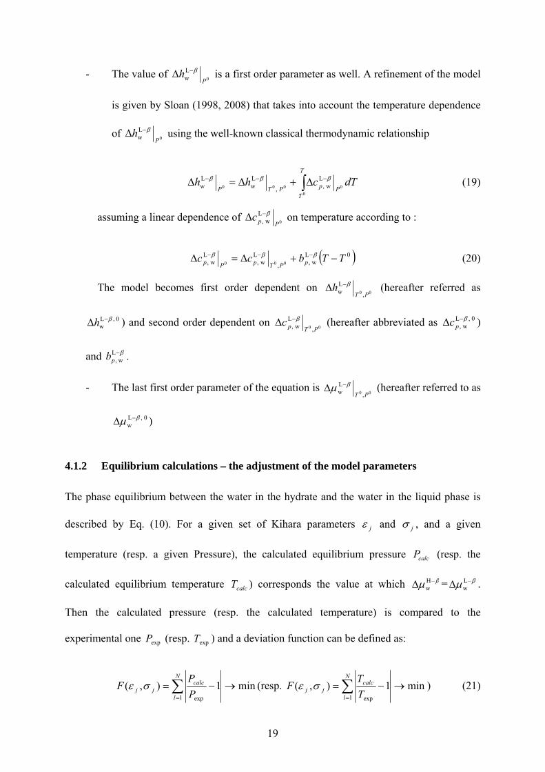
h β−Δ is a first order parame ell. A refinement of the model

is given by Sloan (1998, 200

ter as w

8) that takes into account the temperature dependence

of 0

Lw P

h β−Δ using the well-known classical thermodynamic relationship

∫ −−− Δ+Δ=ΔT

TPpPTP

00000 w,,ww dTchh LLL βββ (19)

assuming a linear dependence of

0

Lw, Ppc β−Δ on temperature according to :

( )0Lw,,

Lw,

Lw, 000 TTbcc pPTpPp −+Δ=Δ −−− βββ (20)

The model becomes first order dependent on 00 ,

L β−w PT

hΔ (hereafter referred as

) and second order dependent on 0,Lw

β−Δh 00 ,

Lw, PTpc β−Δ (herea

and

- T quation is

fter abbreviated as 0,Lw,β−Δ pc )

β−L .

he last first order parameter of the e

w,pb

00 ,

Lw

βμ −Δ (hereafter refer s

Lw

−

PTred to a

βμΔ )

4.1.2 Equilibrium calculations – the adjustment of the model parameters

The phase equilibrium between the water in the hydrate and the water in the liquid phase is

and a given

0,

described by Eq. (10). For a given set of Kihara parameters jε and jσ ,

temperature (resp. a given Pressure), the calculated equilibrium pressure calcP (resp. the

calculated equilibrium temperature calcT ) corresponds the value which β−Hwμ = βμ −Δ L

w .

Then the calculated pressure (resp. the calculated temperature) is com

experimental one expP (resp. expT ) and a deviation function can be defined as:

at Δ

pared to the

min1),(1 exp

→−= ∑=

N

l

calcjj P

PF σε (resp. min1),(

1 exp

→−= ∑=

N

l

calcjj T

TF σε ) (21)

19

In Eq. (21), the index l assigns the specific data point and the summation is to be performed

over all N data of the set. Furthermore, the explicit mentioning of the quantitie , s 0,Lw

β−Δh

Tv β−Δ L

w , , and in the argument list of the functional expression for has

been omitted purposely, since these parameters are not the subject and, hence, results of the

imatio

g al relatio

0,Lw,β−Δ pc β−L

w,pb 0,Lw

βμ −Δ

optimisation, but rather have been set previously to fixed values taken from the literature.

Upon introducing the relations given by Eqs. (19) and (20), incorporating the approx n

, and, performin l necessary integrations in the classical thermodynamic n of

Eq. (18), the following equation is derived:

Lw wa x≅

( ) ( )

( )( ) w

0Lw

0w,,w,w,,w

w,0w,w,w0w

ln

12

2

0000

RTppv

TTbTcTbh

TT

T

pPTppPT

ppp

−−Δ+

⎟⎠

⎜⎝

−⎟⎠

⎜⎝

−Δ−+Δ+ (22) 20L0L0LL

0L0,L0L0,LL

1

ln

x

T

TTTbTcTb

⎞⎛⎞⎛

−+Δ−+Δ=Δ

−

−−−−

−−−−−

β

ββββ

βββββ μμ

In Eq. (21), the mole fraction of the water in any equilibrium state is derived by using the

measured results of the mole numbers of both gases i and k in the liquid phase and and

e volume of the liquid phase , respectively, according to

1TT

Ljn L

kn

th LV

( )LLww

Lwkj nnMV

x++

=ρ

(23)

By introducing eq. (14) into the expression of Eq. (13) derived from statistical thermodynamic

considerations, the latter appears in the form

wLV ρ

⎟⎟

⎠⎟⎟⎠

jjj drrkT

2 , (24) ⎞

⎜⎜

⎝

⎛ ⎞⎜⎜⎝

⎛−−=Δ ∑ ∫∑−

j

R

jji

iβ arw

yPTfkT

RT0

Hw

),,,(exp),,(41ln

σεπνμ

ternal parameters of both, eq. (22) and eq. (24),

where ),,,( jjj arw σε is to be replaced by the expressions defined in Eqs. (15) and (16). The

accuracy of the model is dependent on the in

20

as well as on the equation of state used to describe the fugacity of the gas phase. In the next

part, we will adopt the following nomenclature.

The refere

, respectively, as has been outlined above.

fficien

requir

Special att e

correspond

due the diffic

Table 3 su es the values that are allowable and can be found in the open literature as

re entering in this discussion,

- nce parameters (or macroscopic parameters such as 0,Lw

βμ −Δ

and 0,Lw

β−Δh ) will describe the quantities derived directly from classical

thermodynamics. Among these parameters a distinction is made between the first

order and the second order parameters

- The Kihara parameters allow for a rigorous calculation of the Langmuir coe t

ijC , ed in the statistical thermodynamic model for describing the hydrate

phase.

ention has to be paid when assigning values for 0,Lw

βμ −Δ and 0,Lw

β−Δh since th

ing data found in the literature differ strongly from one author to the other, mainly

ulties arising when determining these quantities experimentally. The following

mmariz

cited by Sloan (1998, 2007). However, in Table 3 we report only the authors who have

proposed a complete set of values, for both structures I and II.

Table 6 summarizes the values of the Kihara parameters we obtained following the

optimisation method it is explained later. It can be seen that the kihara parameters are

effectively dependent on 0,Lw

βμ −Δ and 0,Lw

β−Δh and we will see later that the parameters from

Hand and Tse (1986) seems to be the better choice. But befo

another comment can be done which points the difficulty to compare models from authors. In

fact, table 6 gives also the Kihara parameters proposed by Sloan (1998) and Sloan and Koh

(2007). In their model, nd K e implemented 0,Lw

βμ −Δ and 0,Lw

β−Δh from

Dharmawardhana et al (1980). We can see firstly that values of the Kihara parameters have

been modified from 1998 to 2007. Secondly, we can see the values differ from the kihara

Sloan a oh hav

21

parameters we regressed in our work by using also the reference parameters from

Dharmawardhana et al (1980). It underlines the difficulty to c the mo tween

authors because two many points need to be clarified: what are the data on which the models

are regressed? What is the method retained in the integration of the cell potential? Do the

model have the same reference parameters? So, the comparison between models can not be

done by comparing their internal parameters or Kihara parameters, but by comparing the

precision of their simulation from a common experimental data base. It is not the purpose of

this publication which aims at choosing the best set of 0,Lw

βμ −Δ and 0,Lw

β−Δh parameters.

Table 3 Mascroscopic parameters of hydrates and Ice from Sloan (1998, 2007)

ompare dels be

Structure I Structure II 0,L

wβμ − 0,I

wβ−Δh 0,L

wβμ −Δ 0,I

wβ−Δh Δ

J/mol J/mol J/mol J/mol 6 atteeuw99 0 820 0 van der nd Pl (1959) Waals a1255.2 753 795 837 Child (1964) 1297 1389 937 1025 Dharmawardhana et al (1980)..........model 1(*)1 ..model 2(*)120 931 1714 1400 John et al (1985) ............................1 ...model 3(*)287 931 1068 764 Handa and Tse (1986)...................

60110,Iw

0, Δ= −ββ hLw −Δ −h , where 6011 is the enthalpy of fusion of Ice (J/mol)

(*) model refers to the model in w h the βμΔ and reference parameters are ented as described i xt pa w

0,L 0,Lw

β−Δhw

rt o the

−hicimplem n e the n f ork.

The Kihara eters have been d ined

ure and rium data of p

ters are ndent β− and

art of the work, we will evaluate the

performance of three models. Model 1 is the model implemented with and

from Dharmawardhana et al (1980), model 2 is implemented with values from John et

al (1985) and model 3 is implemented with values from Handa and Tse (1986).

param eterm by fitting the experimental data (mainly

press temperature equilib ure components) and assuming one type of

structure. Therefore, the Kihara parame depe on the values of wμΔ

0,L β−h which have been retained. In the next p

0,L

wΔ

0,Lw

βμ −Δ

0,Lw

β−Δh

22

Table 4 Reference properties of hydrates from Sloan (1998, 2007)

Unit Structure I Structure II 0,L

wβ−Δh J mol SI,,

Iw 00 PT

h β−Δ -6011 SII,,

Iw 00 PT

h β−Δ -6011

0

Lw T

v β−Δ 10-6 m3/mol 4.5959 4.99644 0,L

w,β−Δ pc J/(mol K-1) -38.12 -38.12

β−Lw,pb J/(mol K-2) 0.141 0.141

5 Results a d discus

5.1 Determination of the num he hydrates a rium

Experimentally, we can det olum ater (and so the r of moles of water)

which has reacted to form hydrate. This volume is determined from the difference of the

tracer concentration of LiNO3 being present in the liquid phase between the beginning and

mparison between the theoretical hydration number (from model 3, see

Table 5 Experimental and theoretical hydration numbers

Experiment component Peq /MPa Teq/K

n sion

hydration ber of t t equilib

ermine the v e of w numbe

equilibrium (Eq.6).

The quantities of gases which have been incorporated into the lattice structure of the hydrate

is calculated from a mass balance Eq. (1). Proceeding in this way we can evaluate the

hydration number of the respective hydrate at equilibrium.

Table 5 shows a co

following) and the experimental one, assuming that structure I is formed. The data reveal a

good correlation for the pure gas hydrates of CO2 and CH4 and a less good one for the case of

the CO2-N2 gas hydrate.

Experimental Hydration number

Calculated Hydration number(*)

1 CO2 1.70 275.6 6.35 6.2 2 CO2 1.45 274.6 6.23 6.2 3 CO2 1.57 274.8 6.65 6.2 4 CH4 3.40 275.8 6.29 6.0 5 CH 2.83 273.8 6.14 6.1 46 CH4 2.86 273 6.09 6.0

23

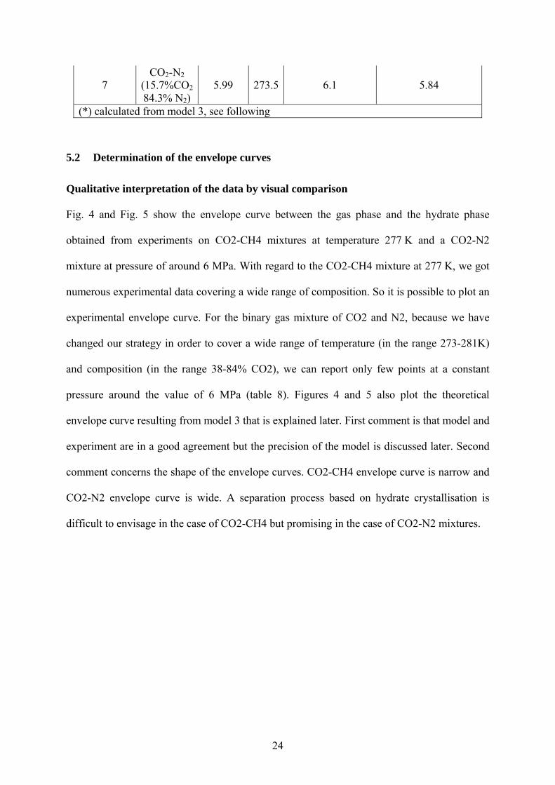
7 CO2-N2

(15.7%CO2 84.3% N2)

5.99 273.5 6.1 5.84

(*) c ulated fro del 3, s lowalc m mo ee fol ing

5.2 D rminatio he env cu

Qualita e inte f th a b al compa

Fig between the gas phase and the hydrate phase

obtained from experiments on CO2-CH4 mixtures at temperature 277 K and a CO2-N2

ard to the CO2-CH4 mixture at 277 K, we got

ion. So it is possible to plot an

ete n of t elope rves

tiv rpretation o e dat y visu rison

. 4 and Fig. 5 show the envelope curve

mixture at pressure of around 6 MPa. With reg

numerous experimental data covering a wide range of composit

experimental envelope curve. For the binary gas mixture of CO2 and N2, because we have

changed our strategy in order to cover a wide range of temperature (in the range 273-281K)

and composition (in the range 38-84% CO2), we can report only few points at a constant

pressure around the value of 6 MPa (table 8). Figures 4 and 5 also plot the theoretical

envelope curve resulting from model 3 that is explained later. First comment is that model and

experiment are in a good agreement but the precision of the model is discussed later. Second

comment concerns the shape of the envelope curves. CO2-CH4 envelope curve is narrow and

CO2-N2 envelope curve is wide. A separation process based on hydrate crystallisation is

difficult to envisage in the case of CO2-CH4 but promising in the case of CO2-N2 mixtures.

24

T=4°C

1,5

2

2,5

3

3,5

4

4,5

0 0,2 0,4 0,6 0,8 1

xCO2

Peq

[Mpa

]

xCO2-GasxCO2-Hyd

Fig. 4 Gas hydrate phase diagram for CO2-CH4 gas mixture at 277 K. x-axis is the molar composition of the gas or hydrate phase (xCO2 + xCH4 = 1) and y-axis is the equilibrium pressure

P=[5.9-6.1] MPa

-30

-25

-20

-15

-10

-5

0

5

10

15

0 0,2 0,4 0,6 0,8 1

xCO2

Teq

[°C

]

xCO2-GasxCO2-Hyd

hypothetical part of the curve,temperature of waterbeing inferior to 0°C

Fig. 5 Gas hydrate phase diagram for CO2-N2 gas mixture at pressure of [5.9-6.1 MPa]. x-axis is the molar composition of the gas or hydrate phase (xCO2 + xN2 = 1) and y-axis is the equilibrium temperature.

Procedure to determine the best set of internal parameters

The classical van der Waals and Platteeuw model (1959) is dependent on its internal

parameters: the reference parameters (or macroscopic parameters) are coming from relations

25

obtained from classical thermodynamics (Eq. 19), whereas the Kihara parameters (Ea. 15 and

16) allow for modelling the Langmuir coefficients (Eq. 14).

Our procedure for selecting the best set of internal parameters consists of initially choosing a

set of macroscopic parameters from literature (Table 3), followed by an optimisation of the

Kihara parameters such that the mean standard deviation between the results calculated by the

model equations and selected experimental results is minimized. It results in three different

models called model 1, model 2 and model 3. Finally, we retain the best set of parameters (2

macroscopic parameters + 3 optimized Kihara parameters) which is the one belonging to the

lower mean standard deviation. In detail, the following procedure is applied:

Stage 1: determination of the best set of macroscopic parameters

1) Choice of a set of macroscopic parameters from Table 3.

2) Under the assumption of a SI and SII structure, respectively, retrieving the best

Kihara parameters by adjusting ε, σ and a to minimize the mean standard

deviation between the experimental data and the corresponding data calculated

from the model (Tables 7, 8 and 9)

i. Calculation of the mean standard deviation for the pressure and

temperature equilibrium data in case of the systems containing only a

single gaseous component (CO2, CH4 and N2) (data from the literature)

ii. Calculation of the mean standard deviation of pressure, temperature

and hydrate composition from our experimental data for the CO2-CH4

and CO2-N2 mixtures

3) Validation of the set of optimised parameters with the experimental results

from Jhaveri and Robinson (1965) who give a complete set of data on the

equilibrium pressure and hydrate composition of the binary CH4-N2 hydrate

(Table 10).

26

Stage 2: following stage 1, we got three sets of optimised Kihara parameters, based on three

sets of macroscopic parameters following the values given by Dharmawardhana et al. (1980),

John et al. (1985) and Handa and Tse (1986) in Table 3. Subsequently, each set of parameters

(2 macroscopic parameters + 3 Kihara parameters) is implemented in the van der Waals and

Platteeuw model (1959) and we compare the experimental results with data available in the

literature. We found two publications, one of Seo et al. (2000) in which both binary gas

mixtures, the CO2-N2 as well as the CO2-CH4 mixture, are studied, and a work of Kang et al.

(2000) in which the binary mixture CO2-N2 is studied (Tables 11, 13, and 14, respectively).

%10min ±σ

%10min

±kε

30%

30%

%10min ±σ%10

min

±kε

Fig. 6 Typical shape of the deviation (average deviation of the equilibrium pressure) between the model and the experimental results as a function of the Kihara parameters. x and y axes correspond respectively to kihara parameters σ and ε which are varied plus or minus 10% around their best value. The best set of value σ and ε is the one that minimises the objective function F (in equation 21)

Special comment on step 2 of stage 1: From a numerical point of view, the determination of

the best set of Kihara parameters (given a set of macroscopic parameters) is time consuming.

In fact, in Fig. 6 the typical shape of a surface plot of the objective function, giving the

deviation between the modelled data to the experimental data, versus the Kihara parameters is

shown. In this example, the experimental results concern the hydrate equilibrium

corresponding to pure CO2 (Adisasmito et al., 1991, reference (b) in Table 7) and the model is

27

implemented with macroscopic parameters from Handa and Tse (see Table 3). The average

deviation is calculated from the 9 experimental equilibrium pressures and the 9 calculated

pressures (called ADi in Table 7). We varied kε and σ around its best value (see Table 7) in

the range plus or minus 10%. It can be noticed from Fig. 6 that the minimum is localised in a

deep but flat bottom valley on which the algorithm of minimisation need to move slowly.

Stages 1.1 and 1.2: Choice of a set of macroscopic parameters from andTable 3

determination of the best set of Kihara parameters to fit with experimental results

Table 8 and Table 9 give the comparison between our experimental results and the results of

the model using the optimised set of Kihara parameters with the three sets of macroscopic

parameters (Table 3) being implemented in the model from Dharmawardhana et al. (1980),

John et al. (1985) and Handa and Tse (1986). For each set of macroscopic parameters, we

have optimised the Kihara parameters, and the results are given in

28

Table 6. Tables 7 and 8 present the experimental points (pressure, temperature, gas

composition, and hydrate composition) on the left part. The mid-column indicates the

structure that is presented as the most stable one from the model. The right part of the table

shows the results of the simulation for the best set of reference parameters (which turns out to

be the parameters from Handa and Tse (1986): we present the calculated values of pressure

and composition, and additionally the deviation between calculated and measured results. At

the bottom of the table the average deviation from the three sets of macroscopic parameters

from Dharmawardhana et al. (1980), John et al. (1985) and Handa and Tse (1986) is

presented. The models have been run with an optimised set of Kihara parameters which are

recapitulated in

29

Table 6.

Table 7 shows the comparison of models with experiments on (CO2-CH4) mixtures (this

study). All the models reveal to be very efficient, both with regard to the estimation of the

equilibrium pressure as well as the hydrate composition. At that level of the presentation, it is

difficult to underline/identify the best model description. The best model description seems to

be the one using Kihara parameters that have been fitted after implementation of the reference

properties from Handa and Tse (1986). The average deviation for this case amounts to 3% for

the calculation of the equilibrium pressure, and a remarkable good evaluation of the gas

composition, both for the CO2 (deviation of 0.6%) and the CH4 system (deviation of 1.25%),

has been attained. The situation changes completely if we take a look at the CO2-N2 mixture.

The Kihara parameters regressed on the data of the hydrate equilibrium involving N2 as a

single gas under the assumption of a SII structure (see Table 7) is implemented in the model.

The corresponding results are compared with our experimental results. Using the reference

properties from Dharmawardhana et al. (1980) or John et al. (1985), the model fails in

simulating the experimental data. With the reference properties from Handa and Tse (1986) as

given in Table 3, and optimised Kihara parameters from

30

Table 6 (this study), we observe a good agreement between the model and the experiments,

with respect to the evaluation of both, the equilibrium pressure (average deviation of 8.1%) as

well as the hydrate composition. For the latter we observe an excellent evaluation of the CO2

composition (average deviation of 4.4%) and at least a reasonable evaluation of the N2

composition (average deviation of 10.4%).

31

Table 6 Kihara parameters regressed from experimental results of this study, and Kihara parameters from litterature

Kihara parameters regressed from experimental results of this study and implemented in model 1,2,3 with macroscopic parameters from table 3

(1)Dharmawardhana et al, 1980 - (2) John et al, 1985 – (3) Handa an Tse, 1986

CO2 CH4 N2

kε σ a

kε σ a

kε σ a

Model 1 170.00 2.9855 0.6805 157.85 3.1439 0.3834 126.98 3.0882 0.3526 Model 2 164.56 2.9824 0.6805 154.47 3.1110 0.3834 166.38 3.0978 0.3526 Model 3 171.41 2.9830 0.6805 158.71 3.1503 0.3834 138.22 3.0993 0.3526

Kihara parameters from literature

Sloan, 1998 168.77 2.9818 0.6805 154.54 3.1650 0.3834 125.15 3.0124 0.3526 Sloan, 2007 175..405 2.97638 0.6805 155.593 3.14393 0.3834 127.426 3.13512 0.3526

Stage 1.3: validation of the best set of parameters on experimental results from the

literature for the N2-CH4 equilibrium

The literature presents a large amount of experimental data giving the equilibrium pressure as

a function of the temperature and gas composition, especially for pure gases and binary

components. However, the literature is poor in presenting complete sets of equilibrium data:

pressure, temperature, gas, as well as hydrate composition. Fortunately, the work of Jhaveri

and Robinson (1965) presents such data for the system containing the binary gas mixture N2-

CH4. As we have presented our own experimental results for the CO2-N2 and CO2-CH4

mixtures, the data of Jhaveri and Robinson (1965) are particularly interesting because they

allow for “closing the composition triangle” with the data on the N2-CH4 mixture. The

comparison between the models is presented in Table 10. The best model continues to be the

model 3 (i.e., the Kihara parameters fitted in this work in combination with the reference

properties from Handa and Tse (1986)) with a reasonable average deviation of about 13% for

the evaluation of the equilibrium pressure, and a deviation of about 10% for the evaluation of

the hydrate composition.

32

So, at this intermediate level of the discussion, we can asses that we dispose of a reliable

model (model 3) to predict both binary mixtures and pure gas equilibrium of gases composed

from the CO2, CH4, N2 elements. Nevertheless, we do not have data to validate the model 3

for the ternary system CO2 + CH4 + N2.

Table 7 Experimental data and comparison to models for CO2 and CH4 and CO2-CH4 gas hydrates

Experiment Structure Simulation Gas Hydrate Pressure Hydrate

T PeqMolar

fraction Molar

fraction Peq Molar fraction 0.06 ± °C MPa CO2 CH4 CO2 CH4 MPa %D3 CO2 %D3 CH4 %D3

(a) 4.00 2.04 1.00 0.00 1.00 0.00 SI 2.00 1.92 1.00 0.00 0.00 0.00 (a) 4.00 2.36 0.64 0.36 0.77 0.23 SI 2.32 1.72 0.76 1.16 0.24 3.83 (a) 4.00 2.55 0.52 0.48 0.68 0.32 SI 2.47 3.15 0.67 1.09 0.33 2.28 (a) 4.00 2.80 0.36 0.64 0.54 0.46 SI 2.74 2.18 0.53 1.17 0.47 1.34 (a) 4.00 3.55 0.11 0.89 0.21 0.79 SI 3.39 4.56 0.21 0.20 0.79 0.06 (a) 4.00 3.90 0.00 1.00 0.00 1.00 SI 3.88 0.59 0.00 0.00 1.00 0.00 (b) 0.15 1.42 1 0 1 0 SI 1.27 10.25 1 0 (b) 2.35 1.63 1 0 1 0 SI 1.64 0.83 1 0 (b) 3.65 1.90 1 0 1 0 SI 1.92 0.93 1 0 (b) 4.45 2.11 1 0 1 0 SI 2.11 0.17 1 0 (b) 5.95 2.55 1 0 1 0 SI 2.55 0.04 1 0 (b) 7.45 3.12 1 0 1 0 SI 3.11 0.29 1 0 (b) 8.35 3.51 1 0 1 0 SI 3.53 0.70 1 0 (b) 8.95 3.81 1 0 1 0 SI 3.87 1.50 1 0 (b) 9.75 4.37 1 0 1 0 SI 4.37 0.01 1 0 (c) 0.25 2.68 0 1 0 1 SI 2.63 1.94 0 1 (c) 1.45 3.05 0 1 0 1 SI 2.97 2.67 0 1 (c) 3.55 3.72 0 1 0 1 SI 3.70 0.62 0 1 (c) 5.15 4.39 0 1 0 1 SI 4.37 0.46 0 1 (c) 6.45 5.02 0 1 0 1 SI 5.05 0.61 0 1 (c) 7.75 5.77 0 1 0 1 SI 5.83 0.97 0 1 (c) 9.15 6.65 0 1 0 1 SI 6.90 3.80 0 1 (c) 10.45 7.59 0 1 0 1 SI 8.11 6.80 0 1 (c) 11.55 8.55 0 1 0 1 SI 9.34 9.25 0 1 (c) 12.55 9.17 0 1 0 1 SI 10.73 17.06 0 1 (c) 13.25 10.57 0 1 0 1 SI 11.87 12.34 0 1

AD1 2.22 1.15 2.46 AD2 3.16 1.67 3.14 AD3 3.04 0.60 1.25

For each line, an individual deviation called %D3 is evaluated between experimental data and model implemented with reference properties from (3) ADi is an average deviation referring to models i=1..3 in which reference properties are from (1)Dharmawardhana et al (1980) - (2) John et al (1985) – (3) Handa and Tse (1986) (a) experimental equilibrium data from this study (b) and (c) experimental equilibrium data from Adisasmito et al, 1991

33

Table 8 Experimental data and comparison to models for CO2- N2 gas hydrates Experiment Structure Simulation

Gas Hydrate Pressure Hydrate

°C MPa Molar fraction

Molar fraction MPa Molar fraction 0.06 ±

T Peq CO2 N2 CO2 N2 Peq %D3 CO2 %D3 N2 %D3 (a) 0.25 6.10 0.16 0.84 0.66 0.34 SI 5.79 5.01 0.59 10.20 0.41 19.62 (a) 1.35 6.20 0.16 0.84 0.66 0.34 SI 6.49 4.70 0.59 9.86 0.41 18.89 (a) 2.25 6.40 0.19 0.82 0.66 0.34 SI 6.73 5.13 0.62 6.08 0.38 11.60 (a) 3.35 6.60 0.20 0.80 0.58 0.42 SI 7.41 12.26 0.63 7.13 0.37 10.02 (a) 0.75 5.90 0.25 0.75 0.75 0.25 SI 4.38 25.74 0.71 5.42 0.29 16.43 (a) 1.55 5.90 0.26 0.75 0.73 0.27 SI 4.82 18.29 0.71 3.08 0.29 8.33 (a) 2.85 5.90 0.26 0.74 0.70 0.30 SI 5.57 5.54 0.71 0.17 0.29 0.41 (a) 3.75 6.00 0.27 0.74 0.70 0.30 SI 6.29 4.76 0.70 0.58 0.30 1.38 (a) 4.65 6.30 0.29 0.71 0.67 0.33 SI 6.62 5.04 0.72 6.59 0.28 13.43 (a) 4.95 6.40 0.30 0.71 0.69 0.31 SI 6.84 6.87 0.72 3.58 0.28 8.01 (a) 5.25 6.40 0.30 0.71 0.72 0.29 SI 7.17 12.06 0.71 0.38 0.29 0.96 (a) 5.45 6.50 0.30 0.70 0.70 0.31 SI 7.27 11.80 0.72 2.96 0.28 6.74 (a) 2.25 6.10 0.20 0.80 0.67 0.33 SI 6.29 3.04 0.64 4.25 0.36 8.64 (a) 2.85 6.20 0.22 0.78 0.65 0.35 SI 6.44 3.93 0.66 1.26 0.34 2.33 (a) 6.95 5.30 0.56 0.44 0.85 0.16 SI 5.17 2.47 0.87 2.40 0.13 13.08 (a) 7.95 5.60 0.59 0.42 0.82 0.18 SI 5.79 3.47 0.87 6.14 0.13 27.80

AD1 39.18 10.31 25.20 AD2 70.81 53.67 127.3 AD3 8.13 4.38 10.38 For each line, an individual deviation called %D3 is evaluated between experimental data and model implemented with reference properties from (3) ADi is an average deviation referring to models i=1..3 in which reference properties are from (1)Dharmawardhana et al (1980) - (2) John et al (1985) – (3) Handa and Tse (1986) (a) experimental equilibrium data from this study

34

Table 9 Experimental data from literature and comparison with model for N2 gas hydrates Experiment Simulations

Model 3 Model 2 Model 1 Simulated Simulated Simulated °C MPa Pressure Pressure Pressure T Peq MPa %D3 MPa %D2 MPa %D1

(d) 0.05 16.01 13.17 17.72 13.62 14.96 13.63 14.86 (d) 0.05 16.31 13.17 19.24 13.62 16.52 13.63 16.42 (d) 0.25 16.62 13.49 20.74 13.93 16.17 13.93 16.17 (d) 0.85 17.53 14.50 23.05 14.95 14.74 14.98 14.56 (d) 1.05 17.73 14.85 18.21 15.29 13.74 15.33 13.56 (d) 1.65 19.15 15.99 22.45 16.43 14.18 16.50 13.81 (d) 1.65 19.25 15.99 16.93 16.43 14.63 16.50 14.26 (d) 2.05 19.66 16.78 18.67 17.23 12.38 17.32 11.90 (d) 2.45 20.67 17.67 18.81 18.11 12.38 18.18 12.07 (d) 2.65 21.58 18.11 18.13 18.56 14.02 18.65 13.58 (d) 3.05 22.39 19.06 19.11 19.25 14.02 19.62 12.39 (d) 3.45 23.1 20.06 17.48 20.49 11.31 20.61 10.76 (d) 4.05 24.83 21.66 19.21 22.10 10.99 22.26 10.35 (d) 5.05 27.36 24.70 20.84 25.11 8.23 25.32 7.47 (d) 5.05 27.97 24.70 11.70 25.11 10.23 25.32 9.49 (d) 5.45 28.27 26.06 12.64 26.44 6.48 26.66 5.69 (d) 6.05 29.89 28.24 12.82 28.56 4.45 28.85 3.49 (d) 6.05 30.3 28.24 6.78 28.56 5.74 28.85 4.80 (d) 7.05 33.94 32.33 16.78 32.55 4.09 32.42 4.47 (d) 8.05 37.49 37.05 13.77 36.98 1.35 37.49 0.00 (d) 8.45 38.61 39.14 4.05 39.26 1.69 39.64 2.68 (d) 9.05 41.44 42.49 5.56 41.54 0.25 42.94 3.61 (d) 10.05 45.9 48.76 7.42 48.64 5.96 49.14 7.06 (d) 11.05 50.66 55.98 3.75 55.60 9.76 56.17 10.88 (d) 11.45 52.29 59.15 7.06 57.76 10.45 59.28 13.36 (d) 12.05 55.43 64.28 6.71 63.58 14.71 64.21 15.85 (d) 13.05 61.4 73.71 4.69 71.94 17.17 72.95 18.82 (d) 14.05 67.79 84.73 8.74 83.09 22.56 83.85 23.69 (d) 14.65 71.23 92.08 18.96 90.18 26.60 90.69 27.31 (d) 15.25 74.58 100.1 23.46 98.29 31.78 98.54 32.12 (d) 16.05 81.47 112.0 22.82 109.4 34.32 109.6 34.63 (d) 17.05 89.37 128.7 25.28 126.1 41.15 125.4 40.59 (d) 17.45 92.21 136.7 39.55 133.7 45.05 132.3 43.95 (d) 17.85 95.86 144.8 42.70 140.8 46.92 140.3 46.40

AD1 15.62 AD2 15.74 AD3 16.64

For each line, an individual deviation called %D3 is evaluated between experimental data and model implemented with reference properties from (3) ADi is an average deviation referring to models i=1..3 in which reference properties are from (1) Dharmawardhana et al. (1980) -(2) John et al. (1985) – (3) Handa and Tse (1986) (d) experimental data from van Cleeff and Diepen (1960)

35

Table 10 Experimental data from Jhaveri and Robinson (1986) in comparison with results obtained from model calculations for N2-CH4 gas hydrate

Experiment Structure Simulation Gas Hydrate Pressure Hydrate

T PeqMolar

fraction Molar

fraction Peq Molar fraction

°C MPa N2 CH4 N2 CH4 MPa %D3 N2 %D3 CH4 %D3 (e) 0.05 2.64 0.00 1.00 0.00 1.00 SI 2.58 2.40 0.00 (e) 0.05 3.62 0.16 0.84 0.07 0.94 SI 2.99 17.40 0.04 33.01 0.96 2.30 (e) 0.05 4.31 0.31 0.69 0.10 0.90 SI 3.51 18.45 0.10 0.81 0.90 0.09 (e) 0.05 5.35 0.53 0.47 0.20 0.80 SI 4.73 11.67 0.21 6.97 0.79 1.74 (e) 0.05 6.55 0.65 0.36 0.35 0.65 SI 5.75 12.26 0.31 12.52 0.69 6.74 (e) 0.05 7.75 0.73 0.28 0.43 0.58 SI 6.74 12.97 0.39 7.79 0.61 5.76 (e) 0.05 10.64 0.82 0.19 0.62 0.38 SI 8.37 21.36 0.52 15.94 0.48 26.01 (e) 0.05 11.65 0.88 0.12 0.71 0.29 SI 10.07 13.57 0.65 8.89 0.35 21.77 (e) 0.05 12.77 0.90 0.10 0.77 0.24 SII 10.61 16.93 0.77 1.00 0.23 3.24 (e) 4.25 3.86 0.00 1.00 0.00 1.00 SI 3.98 3.15 0.00 (e) 4.25 5.20 0.44 0.56 0.18 0.82 SI 6.59 26.66 0.17 5.87 0.83 1.29 (e) 4.25 8.11 0.63 0.37 0.31 0.69 SI 9.07 11.86 0.31 0.19 0.69 0.08 (e) 4.25 10.34 0.74 0.26 0.47 0.53 SI 11.50 11.24 0.43 7.72 0.57 6.85 (e) 4.25 12.06 0.78 0.22 0.56 0.44 SI 12.70 5.28 0.49 12.48 0.51 15.89 (e) 4.25 13.32 0.93 0.07 0.81 0.19 SII 18.90 41.92 0.84 3.37 0.16 14.38 (e) 4.25 14.59 0.94 0.06 0.86 0.14 SII 19.51 33.69 0.87 0.86 0.13 5.26 (e) 4.25 16.21 1.00 0.00 1.00 0.00 SII 22.23 37.13 1.00 (e) 6.65 5.14 0.00 1.00 0.00 1.00 SI 5.17 0.57 0.00 (e) 6.65 7.14 0.35 0.65 0.09 0.91 SI 7.69 7.76 0.13 40.58 0.87 4.06 (e) 6.65 8.37 0.46 0.54 0.22 0.78 SI 9.06 8.29 0.19 15.14 0.81 4.37 (e) 6.65 15.55 0.75 0.25 0.55 0.45 SI 16.16 3.95 0.46 15.68 0.54 19.16 (e) 6.65 20.67 0.84 0.16 0.68 0.32 SI 20.58 0.43 0.61 10.86 0.39 23.07 (e) 6.65 25.23 0.91 0.09 0.80 0.20 SII 25.62 1.53 0.82 2.83 0.18 11.47 (e) 6.65 32.42 1.00 0.00 1.00 0.00 SII 30.62 5.55 1.00

AD1 27.50 20.04 23.67 AD2 66.01 123.7 61.82 AD3 13.58 10.66 9.13 For each line, an individual deviation called %D3 is evaluated between experimental data and model implemented with reference properties from (3) ADi is an average deviation referring to models i=1..3 in which reference properties are from (1) Dharmawardhana et al. (1980), (2) John et al. (1985), (3) Handa and Tse (1986) (e) experimental data from Jhaveri and Robinson (1986)

Stage 2: Comparison with other results from the literature

In this part of the work, we are going to compare our experimental results with results from

the literature. At this stage we have optimised, by means of our experimental data, the

parameters of the van der Waals and Platteeuw model (1959) based on using the macroscopic

parameters form Handa and Tse (Table 3) and the Kihara parameters from

36

Table 6. Now, this optimised model is compared with experimental data found in the

literature for the systems composed of the binary gas mixtures CO2-N2 and CO2-CH4. We

have found two publications dealing with these systems, one of Seo et al. (2000) in which

both, the system containing the binary mixture CO2-N2 as well as the one containing CO2-CH4

are studied, and an article of Kang et al. (2000) is which equilibrium data corresponding to the

binary mixture CO2-N2 are reported (Tables 11, 12, and 13). For the CO2-N2 gas mixture,

none of the models is able to predict both, the equilibrium pressure as well as the hydrate

composition, of the experimental results from Seo et al. (2000,

37

Table 11) and Kang et al. (2000, Table 12) with sufficient accuracy. Whereas model 2 is

never efficient, a valuable evaluation of the equilibrium pressure and the CO2 composition is

provided by models 1 and 3, the model 1 of which being the more accurate one. The

equilibrium pressure is evaluated by model 1 with an accuracy of 6.61% and 7.19%,

respectively, for the results of Seo et al. and Kang et al.; in contrast, the accuracy of model 3

amounts to 13.75% and 11.62%, respectively. The CO2 composition is estimated by means of

model 1 with an accuracy of 9.25 and 8.65%, respectively, for the results of Seo et al. and

Kang et al., whereas the accuracy of model 3 is found to be 5.81 and 16.95%, respectively.

The N2 composition is determined by model 1 to within ±19.64 and ±18.96%, respectively,

for the results of Seo et al. and Kang et al., whereas the accuracy of model 3 is respectively

55.16 and 56.40%.

Two intermediate comments can be done.

The first comment concerns the model 3. We need to recall that it allows to feet better than

model 1 and 2 with our data published in this paper (Table 7 and 8 for the mixture CO2-N2

and CO2-CH4) and but also with literature data for CH4-N2 mixture (Table 10). Model 3 is

also valuable in the estimation of pure gas equilibrium. At this step of the work, the model 3

seems self-consistent. But, model 3 fails in estimating the equilibrium of CO2-N2 mixtures

from other sources (Table 11 and 12). A definitive conclusion is our experimental results

differ from literature.

A second comment concerns model 1, which is less efficient than model 3 on our

experimental results (CO2-N2 and CO2-CH4 equilibrium data), but also less efficient for

CH4-N2 equilibrium data from literature. But this model 1 becomes the more efficient for

CO2-N2 mixtures from literature data (Tables 11 and 12). So, the model 1 is partially self-

38

consistent because it models data from literatures for CO2-N2 mixtures, but not CH4-N2.from

literature (Table 10).

For the CO2-CH4 gas mixture (experimental results of Seo et al. (2000), Table 13), only the

equilibrium pressure can be regarded as being well evaluated by model 3 (average deviation

of 7.19%) and model 1 (average deviation of 10.11%). The CO2 composition is in none of the

calculations evaluated well. For CO2 composition in the hydrate phase, an average deviation

of around 35% can be achieved by each of the models. In contrast, the correlation of the mole

fraction of N2 in the hydrate phase fails completely, reflected by an average deviation of some

hundred percents for this quantity by each of the models.

39

Table 11 Experimental data from Seo et al (2000) and comparison to models for

CO2-N2 gas hydrate

Experiment Structure Simulation Gas Hydrate Pressure Hydrate

°C MPa Molar fraction

Molar fraction MPa Molar fraction

T Peq CO2 N2 CO2 N2 Peq %D3 CO2 %D3 N2 %D (f) 0.85 1.39 1.00 0.00 1.00 0.00 SI 1.38 1.19 1.00 0.00 (f) 0.85 1.77 0.82 0.18 0.99 0.02 SI 1.65 6.48 0.97 2.01 0.03 132.1 (f) 0.85 2.35 0.60 0.40 0.95 0.05 SI 2.18 7.19 0.91 4.90 0.09 96.47 (f) 0.85 2.84 0.50 0.50 0.93 0.07 SI 2.54 10.58 0.87 6.48 0.13 86.29 (f) 0.85 3.46 0.40 0.60 0.90 0.10 SI 3.09 10.83 0.82 9.02 0.18 81.27 (f) 0.85 7.24 0.21 0.79 0.58 0.42 SI 5.18 28.44 0.66 12.67 0.34 17.76 (f) 0.85 11.20 0.12 0.88 0.34 0.66 SI 7.60 32.15 0.50 46.42 0.50 24.19 (f) 0.85 14.93 0.05 0.95 0.18 0.82 SI 11.45 23.32 0.29 59.15 0.71 12.92 (f) 0.85 17.93 0.00 1.00 0.00 1.00 SII 14.50 19.10 0.00 1.00 (f) 3.85 1.95 1.00 0.00 1.00 0.00 SI 1.97 0.62 1.00 0.00 (f) 3.85 2.60 0.85 0.15 0.98 0.02 SI 2.29 11.86 0.97 0.98 0.03 43.87 (f) 3.85 3.38 0.59 0.41 0.95 0.05 SI 3.22 4.71 0.89 5.68 0.11 98.59 (f) 3.85 5.23 0.39 0.61 0.89 0.11 SI 4.61 11.96 0.80 10.09 0.20 78.98 (f) 3.85 11.98 0.18 0.82 0.54 0.46 SI 8.77 26.79 0.58 7.95 0.42 9.34 (f) 3.85 15.50 0.12 0.88 0.35 0.65 SI 11.65 24.82 0.46 30.72 0.54 16.73 (f) 3.85 19.17 0.07 0.93 0.19 0.81 SI 15.58 18.75 0.31 61.76 0.69 14.75 (f) 3.85 24.04 0.00 1.00 0.00 1.00 SII 21.12 12.15 0.00 1.00 (f) 6.85 2.80 1.00 0.00 1.00 0.00 SI 2.87 2.45 1.00 0.00 (f) 6.85 3.60 0.83 0.18 0.98 0.02 SI 3.48 3.36 0.96 1.88 0.04 78.27 (f) 6.85 4.23 0.70 0.30 0.96 0.04 SI 4.09 3.32 0.92 4.25 0.08 105.2 (f) 6.85 5.07 0.59 0.41 0.94 0.06 SI 4.82 4.88 0.88 6.70 0.12 111.2 (f) 6.85 8.28 0.39 0.61 0.86 0.14 SI 7.09 14.29 0.77 10.51 0.23 66.86 (f) 6.85 14.97 0.25 0.75 0.64 0.36 SI 10.80 27.89 0.64 0.18 0.36 0.31 (f) 6.85 20.75 0.17 0.83 0.45 0.55 SI 14.80 28.67 0.52 15.82 0.48 12.95 (f) 6.85 26.69 0.09 0.91 0.22 0.78 SI 21.66 18.85 0.34 53.73 0.66 15.30 (f) 6.85 32.31 0.00 1.00 0.00 1.00 SII 31.41 2.78 0.00 1.00

AD1 6.61 9.25 19.64 AD2 61.64 43.31 367.9 AD3 13.75 17.54 55.16 For each line, an individual deviation called %D3 is evaluated between experimental data and model implemented with reference properties from (3) ADi is an average deviation referring to models i=1..3 in which reference properties are from (1)Dharmawardhana et al. (1980) - (2) John et al. (1985) – (3) Handa and Tse (1986) (f) experimental data from from Seo et al. (2000)

40

Table 12 Experimental data from Kang et al. (2001) and comparison to models for CO2-N2 gas hydrate

Experiment Structure Simulation Gas Hydrate Pressure Hydrate

°C MPa Molar fraction

Molar fraction MPa Molar fraction

T Peq CO2 N2 CO2 N2 Peq %D3 CO2 %D3 N2 %D (g) 0.85 1.36 1.00 0.00 1.00 0.00 SI 1.38 1.06 1.00 0.00 (g) 0.85 1.73 0.82 0.18 0.99 0.02 SI 1.65 4.31 0.97 2.01 0.03 132.06 (g) 0.85 2.30 0.60 0.40 0.95 0.05 SI 2.18 4.88 0.91 4.71 0.09 89.48 (g) 0.85 2.77 0.50 0.50 0.93 0.07 SI 2.54 8.51 0.87 6.48 0.13 86.29 (g) 0.85 3.48 0.40 0.60 0.90 0.10 SI 3.09 11.34 0.82 9.02 0.18 81.27 (g) 0.85 7.07 0.21 0.79 0.58 0.42 SI 5.18 26.79 0.66 12.67 0.34 17.76 (g) 0.85 10.95 0.12 0.88 0.34 0.66 SI 7.60 30.59 0.50 46.42 0.50 24.19 (g) 0.85 14.59 0.05 0.95 0.18 0.82 SI 11.45 21.56 0.29 59.15 0.71 12.92 (g) 0.85 17.52 0.00 1.00 0.00 1.00 SII 14.50 17.24 0.00 1.00 (g) 3.85 1.91 1.00 0.00 1.00 0.00 SI 1.97 2.89 1.00 (g) 3.85 2.54 0.85 0.15 0.98 0.02 SI 2.29 9.78 0.97 1.16 0.03 56.81 (g) 3.85 3.30 0.57 0.43 0.95 0.05 SI 3.32 0.51 0.88 6.48 0.12 112.36 (g) 3.85 5.12 0.39 0.61 0.89 0.11 SI 4.61 10.02 0.80 10.09 0.20 78.98 (g) 3.85 11.71 0.18 0.82 0.54 0.46 SI 8.77 25.10 0.58 7.95 0.42 9.34 (g) 3.85 15.15 0.12 0.88 0.35 0.65 SI 11.40 24.76 0.47 33.30 0.53 18.14 (g) 3.85 18.74 0.07 0.93 0.19 0.81 SI 15.58 16.87 0.31 61.76 0.69 14.75 (g) 3.85 23.50 0.00 1.00 0.00 1.00 SII 21.12 10.13 0.00 1.00 (g) 3.85 1.91 1.00 0.00 1.00 0.00 SI 1.97 2.89 1.00 0.00 (g) 3.85 2.54 0.85 0.15 0.98 0.02 SI 2.29 9.78 0.97 1.16 0.03 56.81 (g) 6.85 2.74 1.00 0.00 1.00 0.00 SI 2.87 4.73 1.00 0.00 (g) 6.85 3.52 0.83 0.17 0.98 0.02 SI 3.46 1.72 0.96 2.10 0.04 102.7 (g) 6.85 4.14 0.70 0.30 0.96 0.04 SI 4.09 1.15 0.92 4.13 0.08 99.01 (g) 6.85 4.95 0.59 0.41 0.94 0.06 SI 4.82 2.61 0.88 6.38 0.12 99.94 (g) 6.85 8.09 0.39 0.61 0.86 0.14 SI 7.09 12.33 0.77 10.09 0.23 61.97 (g) 6.85 14.64 0.25 0.75 0.64 0.36 SI 10.80 26.25 0.64 0.18 0.36 0.31 (g) 6.85 20.29 0.17 0.83 0.45 0.55 SI 14.80 27.04 0.52 15.82 0.48 12.95 (g) 6.85 26.09 0.09 0.91 0.22 0.78 SI 21.66 16.99 0.34 54.91 0.66 15.49 (g) 6.85 31.58 0.00 1.00 0.00 1.00 SII 31.41 0.54 0.00 1.00 (g) 6.85 2.74 1.00 0.00 1.00 0.00 SI 2.87 4.73 1.00 0.00

AD1 7.19 8.69 18.96 AD2 55.89 41.97 393.2 AD3 11.62 16.95 56.40 For each line, an individual deviation called %D3 is evaluated between experimental data and model implemented with reference properties from (3) ADi is an average deviation referring to models i=1..3 in which reference properties are from (1) Dharmawardhana et al. (1980) - (2) John et al. (1985) – (3) Handa and Tse (1986) (g) experimental data from Kang et al (2000)

41

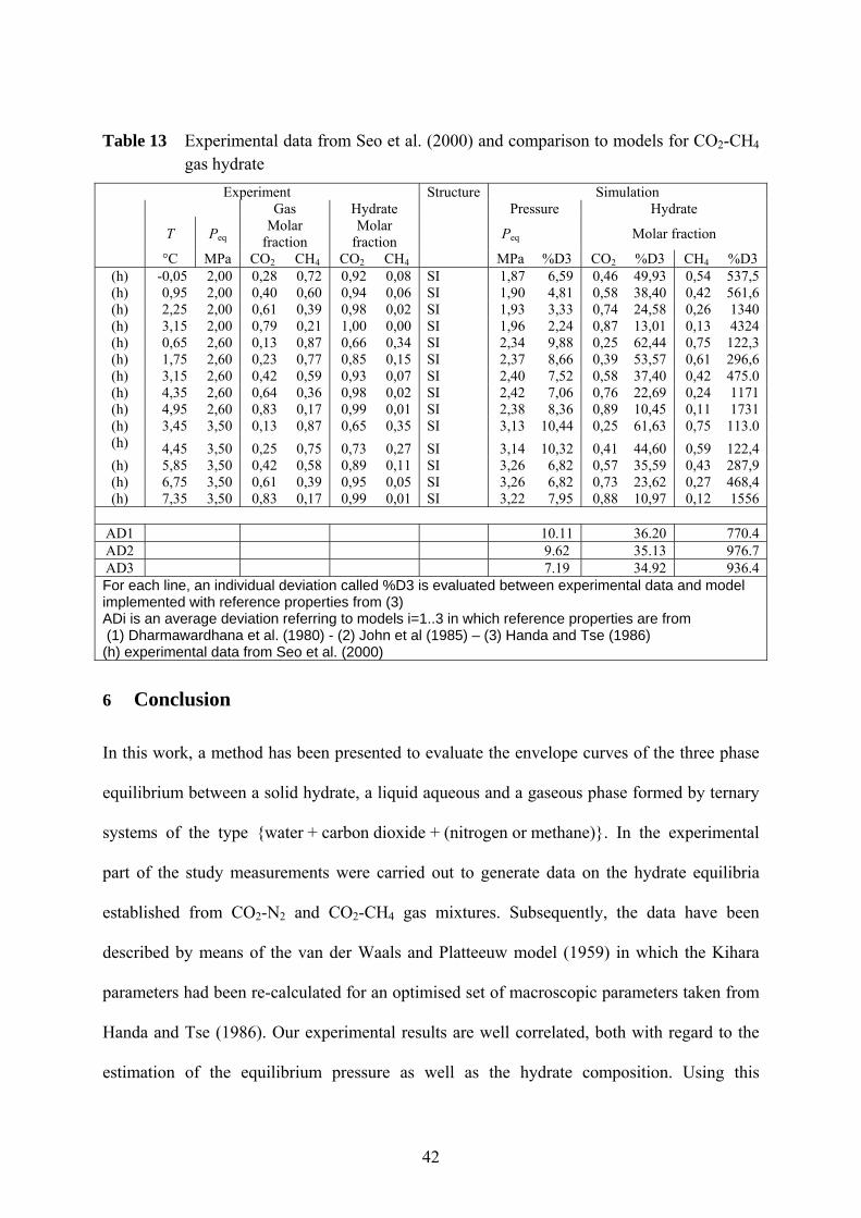
Table 13 Experimental data from Seo et al. (2000) and comparison to models for CO2-CH4 gas hydrate

Experiment Structure Simulation Gas Hydrate Pressure Hydrate

T Peq Molar

fraction Molar

fraction Peq Molar fraction

°C MPa CO2 CH4 CO2 CH4 MPa %D3 CO2 %D3 CH4 %D3 (h) -0,05 2,00 0,28 0,72 0,92 0,08 SI 1,87 6,59 0,46 49,93 0,54 537,5 (h) 0,95 2,00 0,40 0,60 0,94 0,06 SI 1,90 4,81 0,58 38,40 0,42 561,6 (h) 2,25 2,00 0,61 0,39 0,98 0,02 SI 1,93 3,33 0,74 24,58 0,26 1340 (h) 3,15 2,00 0,79 0,21 1,00 0,00 SI 1,96 2,24 0,87 13,01 0,13 4324 (h) 0,65 2,60 0,13 0,87 0,66 0,34 SI 2,34 9,88 0,25 62,44 0,75 122,3 (h) 1,75 2,60 0,23 0,77 0,85 0,15 SI 2,37 8,66 0,39 53,57 0,61 296,6 (h) 3,15 2,60 0,42 0,59 0,93 0,07 SI 2,40 7,52 0,58 37,40 0,42 475.0 (h) 4,35 2,60 0,64 0,36 0,98 0,02 SI 2,42 7,06 0,76 22,69 0,24 1171 (h) 4,95 2,60 0,83 0,17 0,99 0,01 SI 2,38 8,36 0,89 10,45 0,11 1731 (h) 3,45 3,50 0,13 0,87 0,65 0,35 SI 3,13 10,44 0,25 61,63 0,75 113.0 (h) 4,45 3,50 0,25 0,75 0,73 0,27 SI 3,14 10,32 0,41 44,60 0,59 122,4 (h) 5,85 3,50 0,42 0,58 0,89 0,11 SI 3,26 6,82 0,57 35,59 0,43 287,9 (h) 6,75 3,50 0,61 0,39 0,95 0,05 SI 3,26 6,82 0,73 23,62 0,27 468,4 (h) 7,35 3,50 0,83 0,17 0,99 0,01 SI 3,22 7,95 0,88 10,97 0,12 1556

AD1 10.11 36.20 770.4 AD2 9.62 35.13 976.7 AD3 7.19 34.92 936.4 For each line, an individual deviation called %D3 is evaluated between experimental data and model implemented with reference properties from (3) ADi is an average deviation referring to models i=1..3 in which reference properties are from (1) Dharmawardhana et al. (1980) - (2) John et al (1985) – (3) Handa and Tse (1986) (h) experimental data from Seo et al. (2000)

6 Conclusion

In this work, a method has been presented to evaluate the envelope curves of the three phase

equilibrium between a solid hydrate, a liquid aqueous and a gaseous phase formed by ternary

systems of the type {water + carbon dioxide + (nitrogen or methane)}. In the experimental

part of the study measurements were carried out to generate data on the hydrate equilibria

established from CO2-N2 and CO2-CH4 gas mixtures. Subsequently, the data have been

described by means of the van der Waals and Platteeuw model (1959) in which the Kihara

parameters had been re-calculated for an optimised set of macroscopic parameters taken from

Handa and Tse (1986). Our experimental results are well correlated, both with regard to the

estimation of the equilibrium pressure as well as the hydrate composition. Using this

42

optimised set of parameters, the model has been validated against experimental results found

in the literature. At first the model had been tested against data of the system

{H2O + N2 + CH4}, a mixture not being investigated experimentally in this work. It turned out

that the model continues to work efficiently, with regard to the estimation of both, the

pressure as well as the hydrate composition. Finally, the performance of the model was tested

against measured data from the literature for the systems composed of the same gas mixtures

we have tested, i.e. CO2-N2 and CO2-CH4. Depending on the source of the data (Seo et al.

(2000) or Kang et al. (2001)), our modelled results deviate slightly or strongly from the

literature results. Whereas the equilibrium pressure is estimated correctly by our model (with

a standard deviation ranging from 7 to 13%), the hydrate composition is never estimated well.

This observation shows that our experimental data differ slightly or strongly from the data of

these authors, too. The main difference concerns the experimental evaluation of the hydrate

composition.

Acknowledgements

This work has been supported by the French Agency for research under the acronym ANR-

CO2 SECOHYA.

The authors thank also all the members of the GasHyDyn team for their constant support and

especially the technical staff : Alain Lallemand, Fabien Chauvy, Richard Drogo and Albert

Boyer

43

Annex 1 : Evaluation of error a) Evaluation of the initial quantity of gases in the reactor from pressure balance. The principle of the preparation of the gases is to generate a binary mixture (for example CO2 and N2) with a given molar composition (z(A) and z(B)) by the following procedure: 0- temperature is controlled to T value 1- After vacuuming, a volume V of reactor (temperature T), inject the first gas (A) into the

reactor up to a pressure P1 2- Inject second gas (B) to a pressure P2 3- Back calculate the molar composition nA, nA+B and nB=nA+B-nA by using the following

algorithm

Calculation of error After convergence, the gas composition is calculated from

( )RTZVPn

PAA

1

1= ; ( )RTZVP

nnPBA

GBA

2

2

++ == and

( )A

PBAB n

RTZVPn −=

+ 2

2

So, a direct evaluation of error on and gives An BAn +

( )

( ) TT

ZZ

VV

PP

nn

PA

PA

A

A Δ+

Δ+

Δ+

Δ=

Δ

1

1

1

1 and ( )

( ) TT

ZZ

VV

PP

nn

PBA

PBA

BA

BA Δ+

Δ+

Δ+

Δ=

Δ

+

+

+

+

1

2

2

2

44

So finally ( )( )( ) A

A

BA

BA

B

B

nn

BzAz

nn

Bznn Δ

+Δ

=Δ

+

+1

- the error on evaluation of pressure is =ΔP 0.05MPa - the error on evaluation of reactor is volume VΔ = 30 cm3 - the error on the valuation of compressibility factor is not evaluated here, and

considered as negligible compared to other - the error on temperature is = 0.1 K TΔ

In regard to the precision of the instrument, the error is mainly due to the precision in the evaluation of the pressure :

1

1

PP

nn

A

A Δ≈

Δ

and

2

2

PP

nn

BA

BA Δ≈

Δ

+

+ and ( )( )( ) A

A

BA

BA

B

B

PP

BzAz

PP

Bznn Δ

+Δ

≈Δ

+

+1

b) Calibration of the gas chromatograph The principle of the preparation of the gases is to generate a binary mixture (for example CO2 and N2) with a given molar composition (z(A) and z(B)), and to compare the ratio (SA/SB) of the surface of the respective chromatograph peak. Once the gas composition is determined, a gas chromatography is performed, and the

respective surface areas ratio of gas A and B ( ( )( )BSAS ) is measured and correlated to ratio of

respective gas composition ( )( )BzAz . The peak surface area is estimated with an error

=0.05.

SS /Δ

The result is a calibration curve which gives estimation of ( )( )BzAz plus or minus 1%.

c) Evaluation of the error on

and ( )Az ( )Bz from gas chromatography

After sampling of the gas phase, once ( )( )BSAS

has been determined by gas chromatography, the

value of ( )( )BzAz

is determined from the previous calibration curve :

45

( )( )BzAza =

and ( ) ( ) 1=+ BzAz ; so ( ) ( )

aaAz

aAz +

=⎟⎠⎞

⎜⎝⎛ +

111 and ( )

aaAz+

=1

So, the error on the evaluation of (or ( )Az ( )Bz ) is ( )( )

( )( ) a

aBzBz

AzAz Δ

=Δ

=Δ 2 and value of 2%

d) Evaluation of the error of the mole number of gas in the gas phase at time t. G

jerrAt time t, the composition of the gas is given form gas chromatography ( zzΔ =0.02) and pressure measurement ( 0.05MPa). =ΔP

TRzpTZVP

nj ),,(RG = and jj znn GG =

j

j

j

j

zz

nn

nn Δ

+Δ

=Δ

G

G

G

G

and PP

nnG

G Δ≈

Δ (see annex 1.a)

With 0.05MPa and =0.02, we obtain an estimation of the error that is always superior to 2%, inferior to 3% as soon as the pressure is superior to 0.5 MPa , and inferior to 2.5% as soon as the pressure is superior to 1 MPa. In our experiments, pressure is always superior to 1 MPa, and we will retain that

=ΔP

=Δ

= G

G

j

jGj n

nerr 0.025

e) Evaluation of the error on the calculation of the gas mole number consumption between two steps at phase at time t1 and t2 We evaluate the error on the calculation of that is the quantity of gas that has been transferred to solution, i.e. dissolution and crystallisation.

GG0 jj nn −

jj

jj

jj zTRzPTZ

VPz

TRzPTZVP

nn),,(),,(

R0

00

R0GG0 −=−

In a good approximation, we can write

( )jjjj zPzPTRZ

Vnn −≈− 00RGG

0 with 2

),,(),,( 00 jj zPTZzPTZZ

+=

Secondly, in consideration that the evaluation of the mole number is first order depend on the precision of pressure P and composition z, we can write

( ) ( )jjjjjj dzPzdPdzPzdPTRZ

Vnnd −−+=− 0000RGG

0

So

( ) ( ) ( )(( )zPPzzPTRZ

Vnn jjjj Δ+++Δ=−Δ 000RGG

0 )

( ) ( )⎟⎟⎠

⎞⎜⎜⎝

⎛Δ+

Δ<

−

−Δz

PP

nnnn

jj

jj 220

0GG

0

GG0 <5%

46

The same calculation can be done for the total amount of gas ( )

0

0GG

0

GG0 2

PP

nnnn Δ

=−

−Δ

f) Evaluation of the error of the mole number of gas in the liquid phase at time t Ljerr

Gas composition of the liquid phase is determined from an Henry correlation (see part 3.3.4, equations 7,8 and 9).

( )RTPvKPy

MV

njj

jjj ∞∞=

exp,H

G

w

wL

L ϕρ

In a first approximation, we can write that

PP

KK

VV

nn

j

j

j

j Δ+

Δ+

Δ=

Δ∞

∞

,H

,HL

L

L

L

with ]Li[]Li[ 0

L0L

+

+

=V

V and so ]Li[]Li[

]Li[]Li[

0

0L

0

L0

L

L

+

+

+

+ Δ+

Δ+

Δ=

ΔVV

VV

<<Δ

L0

L0

VV

0.001 because it is determined from mass measurement, with precision of 0.01g and

total mass of water around 1 kg.

<<Δ

+

+

]Li[]Li[

0.001 in reason of the precision of the ionic chromatography

So, we can give an evaluation of

PP

KK

nn

j

j

j

j Δ+

Δ≈

Δ∞

∞

,H

,HL

L

Without an evaluation of the precision of the Henry constant, we will overestimate it to 10%,

so that ≈Δ

= L

L

j

jLj n

nerr 0.1. We will see after there is no consequence on the evaluation of the

mole number of gas in the hydrate phase (see following) because of low quantity of gas in the liquid phase in respect to the quantity in the gas phase and hydrate phase; g) Evaluation of error of the mole number of gas in the hydrate phase. The mole number of gas in the hydrate phase is calculated from a mass balance from equation (1)

0,GLH jjjj nnnn −+=

In a first approximation, because of the very low solubility of gases in water, we have also Hjj nn << L and 0,

GH jjj nnn −≈So

47

( )

0,G

0,G

H

H

jj

jj

j

j

nnnn

nn

−

−Δ≈

Δ=5% from annex 1.e

h) Evaluation of the error on the calculation of composition (molar fraction) of gas in the hydrate In a first approximation that assumes the quantity of gas in liquid is negligible compared to other quantities (hydrate and gas phases), we can write :

GG0

H

H

H

nnn

nn

x j

ii

jHj −

==∑

( )( GG

0H

2GG0

GG0

H 1 nndnnnnn

dndx j

jHj −

−−

−= ) that gives

( )GG

0

GG0

GG0

H

GG0

H

nnnn

nnn

nnn

x jjHj −

−Δ

−+

−

Δ=Δ

With (annex 1.e) ( )

0

0GG

0

GG0 2

PP

nnnn Δ

=−

−Δwe get 01.005.0

H

Hj

H

HjH

j nn

nn

x +=Δ

So, finally, the evaluation is

06.0<Δ

Hj

Hj

xx

48

Nomenclature/List of symbols

Latin letters:

A Coefficient in correlating equation for Henry’s law constant, and in Parrish and Prausnitz’ equation, respectively

a Activity [-] or Kihara parameter, spherical nucleus radius [m]

B Coefficient in correlating equation for Henry’s law constant [K-1], and in the Parrish and Prausnitz relation, respectively

b Coefficient lineary temperature dependency of the heat capacity [J mol-1 K-2]

C Langmuir constant of cavity

c Molar heat capactiy [J mol-1 K-1]

F Objective function in the difference of the chemical potential differences

f Fugacity [Pa]

h Molar enthalphy [J mol-1]

HK Henry’s constant at saturation pressure of the pure solvent, i.e., at infinite dilution of the gaseous component [Pa-1]

k Boltzmann constant [J K-1]

N Number of points of a given set of data

n Mole number

P Pressure [Pa]

R Gas molecule equivalent radius [m] or universal gas constant [8.314472 m2 kg s-2 K-1 mol-1]

r Distance between the molecule and the wall of the cavity [m]

T Temperature [K]

V Volume [m3]

v (Partial) molar volume [m3 mol-1]

w Potential energy function

x Mole fraction in the liquid or solid phase

y Mole fraction in the gas phase

Z Compressibility factor

z Coordination number of the cavity in which a molecules is enclatrated [-]

Greek letters:

γ Activity coefficient [-]

49

Δ Difference operator

ε Kihara parameter, maximum attraction potential [-]

μ Chemical potential [J mol-1]

ν Number of cavities per molecules of water [-]

θ Occupation rate of cavity/gas

ρ (Mass) Density of water [kg m-3]

σ Kihara parameter, distance between the molecules and the cavity wall, at null potential [m]

Subscripts:

i Index characterising the type of cavities (i = 512, 51262 or 51264)

j, k Index representing component

l Index representing experimental data point l

p Isobaric property

R Index referring to reactor

w Water

0 Referring to initial condition

Superscripts:

I Ice phase

H Hydrate phase

L Liquid phase

G Gas/Vapour phase

β Hypothetical reference phase for the hydrate phase corresponding to empty lattice

βϕ − Referring to the difference between any phase and the reference phase b

∞ Corresponding to the state of infinite dilution

0 Corresponding to reference values for T and/or P

Corresponding to pure component property

References

Adisasmito, S., Frank, R.J., Sloan, E.D, J. Chem. Eng. Data,36, 68, (1991); reference and data from Sloan (2007)

50

Chen, C.-C.; Britt, H. I.; Boston, J. F.; Evans, L.B.; “Local Composition Model for Excess Gibbs Energy of Electrolyte Systems”; AIChE J. 28 (1982) 588-596

Chen, C.-C., Evans, L. B.; “A Local Composition Model for the Excess Gibbs Energy of Aqueous Electrolyte Systems”; AIChE J. 32 (1986) 444-454

Danesh, Ali, PVT and Phase Behaviour of Petroleum Reservoir fluids, Elsevier, 1998

Dharmawandhana, P. B., 1980. The measurement of the thermodynamic parameters of the hydrate structure and application of them in the prediction of natural gas hydrates. PhD Thesis, Colorado School of Mines, Golden, CO.

Holder, G. D., Corbin, G., Papadopoulos, K. D.; Thermodynamic and molecular proprieties of gas hydrates from mixtures containing Methane Argon and Krypton. Ind Eng Chem Fund. 19 (1980) 282

Handa, Y.P.; Tse, J.S. ; J. Phys. Chem. 23 (1986) 5917

Jeffrey, G. A.; Hydrate inclusion compounds. Acad. Press., Vol.1 (1984) 135

Jhaveri, J. and Robinson, D. B.; Can. J. Chem Eng. 43 (1965) 75

John, V. T., and Holder, G. D.; Journal of Physical Chemistry 86, 4 (1982) 455-459

John, V. T., Papadopoulos, K. D., Holder, G. D.; AIChE J. 31 (1985) 252-259

Kang, S. P., Lee, H., Lee, C.-S., Sung, W-M.; Hydrate Phase Equilibria of guest mixtures containing CO2. N2 and Tetrahydrofuran. Fluid Phase Equilibr. 85 (2001) 101-109

Mckoy, V., Sinagoglu, O. J.; Theory of dissociation pressures of some gas hydrates. J Chem. Phys 38 (1963) 2946

Sparks, K.A. and Tester, J.W. ; Intermolecular potential-energy of water clathrates – The inadequacy of the nearest-neigbor approximation, Journal of Physical Chemistry, Vol. 96, 22 (1992) 11022-11029

Mooijer-van den Heuvel, M.M.; Phase Behaviour and Sructural Aspects of ternary clathrate hydrate systems. The role of additives, Ph.D. Thesis, Technische Universiteit Delft (2004)

Munck, J.,. Skjold-Jorgensen, S., Rasmussen, P.; Computations of the formation of gas hydrates; Chem. Eng. Sci. 43 (1988) 2661-2672

Nguyen Hong, D., Chauvy, F. and Herri, J. M.; CO2 Capture by Hydrate crystallization - A potential Solution for Gas Emission of Steelmaking Industry. Energy Conversion and Management; 48 (2007) 1313–1322

51

Parrish, W.R., Prausnitz, J. M.;. Dissociation pressure of gas hydrates formed by gas mixtures. Ind. Eng. Chem. Process Develop. 11 (1972) 26-35

Pitzer, K. S., “Thermodynamics of Electrolytes. I. Theoretical Basis and General Equations”; J. Phys. Chem. 77 (1973) 268-277

Pitzer, K. S., “Electrolytes: From Dilute Solutions to Fused Salts”; J. Am. Chem. Soc. 102 (1980) 2902-2906

Seo, Y-T., Kang, S-P., Lee, C-H., Lee H., Sung, W-M (2000). Hydrate Phase Equilibria for Gas Mixtures Containing Carbon Dioxide: A Proof- of- Concept to Carbon Dioxide Recovery from Multicomponent Gas Stream. Korean Journal of Chemical Engineering. 17 (2000) 659-667

Sherwood, A.E., and Prausnitz, J.M., Chem. Phys., Vol. 41, p. 429, 1964

Sloan, E.D., 1998. Clathrate hydrates of natural gases. 2nd Ed. Marcel Decker. New York

Sloan, E.D., Koh, C.A., 2007. Clathrate hydrates of natural gases. 3nd Ed. CRC Press

Tee, L.S., Gotoh, S., Stewart, W.E., 1996. Molecular Parameters of normal Fluids: The Kihara potential with Special Core. Ind. Eng. Fundam. 5, 363

Thiam, A., 2008. Etude des conditions thermodynamiques et cinétiques du procèdes de captage de CO2 par formation d’hydrates de gaz : Application au mélange CO2-CH4. PhD Thesis. Ecole Nationale Supérieure des Mines de Saint Etienne. France

Uchadin, K.A., Ratcliffe. C.I., Ripmeester, J.A., 2002. Single Crystal Diffraction Studies of Structures I. II and H Hydrates: Structure. Cage Occupancy and Composition. Journal of Supra Molecular Chemistry. Vol.2, pp. 405-408

Van Cleeff, A. and Diepen, G.A.M., Rec.Trav.Chim, 79, 582, 1960 reference and data from Sloan (2007)

Van Der Waals, J.D., 1959. Clathrate solution. Advances in chemical physic. 2, 1-57

Von Stackelberg, M., Muller, H.R., 1951a. On the structure of gas hydrates. J Chem Phys. 1319-1320

52