Gas Dynamics and Kinetics in the Cometary Coma: Theory … · Combi et al.: Gas Dynamics and...

Combi et al.: Gas Dynamics and Kinetics in the Cometary Coma 523

523

Gas Dynamics and Kinetics in the Cometary Coma:Theory and Observations

Michael R. CombiUniversity of Michigan

Walter M. HarrisUniversity of Washington

William H. SmythAtmospheric & Environmental Research, Inc.

Our ability to describe the physical state of the expanding coma affects fundamental areasof cometary study both directly and indirectly. In order to convert measured abundances of gasspecies in the coma to gas production rates, models for the distribution and kinematics of gasspecies in the coma are required. Conversely, many different types of observations, together withlaboratory data and theory, are still required to determine coma model attributes and parameters.Accurate relative and absolute gas production rates and their variations with time and from cometto comet are crucial to our basic understanding of the composition and structure of cometarynuclei and their place in the solar system. We review the gas dynamics and kinetics of cometarycomae from both theoretical and observational perspectives, which are important for understand-ing the wide variety of physical conditions that are encountered.

1. INTRODUCTION

Gases, primarily water, and entrained dust are liberatedfrom the icy nucleus by solar heating when a comet iswithin a few astronomical units (AU) of the Sun and forman outflowing cometary atmosphere. The cometary atmo-sphere, or coma, expands to distances many orders of mag-nitude larger than the size of the nucleus itself. Because ofthe ultimate expansion into vacuum and the very weak grav-ity that affects only the largest dust particles, a Knudsenlayer of a fraction to a few meters in thickness (a few timesthe molecular collision mean free path) forms near the sur-face where the gas organizes itself into a transient stationarythermal layer. The initiation of regular flow transforms thisthermal layer into a rapid transonic dusty-gas flow with atypical scale length of 10–100 m. Expansion and nearly adi-abatic cooling dominates the flow out to scales of ~100 kmwhere the dust becomes decoupled collisionally from thegas. Here the gas flows with a speed of ~700 m s–1 and hasa cool temperature of <30 K. The energetic photochemicalproducts of solar UV photodissociation then begin to heatthe gas faster than it can cool by adiabatic expansion or IRradiational cooling, and the gas kinetic temperature andultimately the outflow speed increase. Photoionization andcharge impact ionization (~5–10% of the photodissociationrate) forms a cometary ionosphere on scales of 103–104 km,which ultimately interacts with the magnetized plasma ofthe solar wind forming an ion tail on scales of 105–107 km.Also, at large scales of 106–107 km, the neutral coma isbroken down into its atomic constituents, such as O, H, C,

and N. This description is most applicable for a typicalcomet observed in the range of a few tenths to about 2 AUfrom the Sun. For comets much farther away, temperaturesand velocities are smaller and reaction length scales arelarger. And for comets much closer (Sun-grazers), tempera-tures and velocities are much larger and reaction lengthscales are smaller.

Our understanding of the conditions within a few timesthe radius of the nucleus results largely from model pre-dictions that are only constrained by the gas fluxes andvelocities hundreds of nucleus-radii from the nucleus, andare determined both by in situ and remote observations.There are not many direct observations about the conditionsnear the surface, beyond the images of 1P/Halley from theGiotto and Vega spacecrafts and those of 19P/Borrelly fromthe Deep Space 1 spacecraft, which show only the dust dis-tribution. This region is described in detail in Crifo et al.(2004). The photodissociation, photoionization and fast ion-neutral chemical reactions involving ultimately ~100 spe-cies and thousands of reactions forms a complex atmos-phere/ionosphere that is described in detail in Rodgers etal. (2004).

The region of the coma accessible by remote ground-based and Earth-orbit-based observations and by direct insitu sampling by spacecraft instrumentations (mostly byneutral gas and plasma mass spectrometers) for detailedstudy generally covers distances larger than a few hundredkilometers from the nucleus. Remote imaging observationsof this region have provided information about the projectedline-of-sight-integrated distribution of neutral gas and ion

524 Comets II

species in two spatial dimensions on the sky plane andsometimes the line-of-sight velocity distribution. Thus re-mote sensing provides somewhat convoluted, nonunique,global views of the coma, whereas in situ measurementshave provided some detailed information about neutral gasand ion densities, velocities, and temperatures, but only fora few fleeting threads along a few spacecraft trajectories.Information about kinetic and rotational temperatures hasbeen obtained by both remote observations and in situ meas-urements. The spectroscopic measurements are discussedin detail in Bockelée-Morvan et al. (2004) (for parent spe-cies) and Feldman et al. (2004) (for nonparent species).

It is important to understand the physical state of thecoma and its variations because it is largely from analysesof observations of various species in the coma that we de-termine the composition of the larger population of com-ets. Although in the last 20 years IR and radio astronomyhave opened the possibility of directly observing parent gasspecies in comets, interpreting these observations is com-plicated by difficult excitation mechanisms, atmosphericextinction (in the IR), and generally weaker signal-to-noisewhen compared with visible and near-UV measurements ofdaughter species. The interpretations of measurements ofdaughter species have their own sets of complicating issuesregarding production models and kinematics. However,routine observations of daughter species in the visible re-mains critically important for the foreseeable future becausethey are more sensitive for weak comets and especially forthose at large heliocentric distances. This is the only prac-tical way to characterize the composition and activity of theentire population of comets and to compare with the largebase of existent data. Observations of daughter species inthe visible should also be made and interpreted side-by-sidewith IR and radio observations of parent species for brightercomets and those at generally smaller heliocentric distancesto enable the entire complex picture to be unraveled.

In this chapter we concentrate on those aspects of photo-chemistry and dynamics that are important for understandingthe overall physical state of the coma, and their variationsfrom comet to comet, with changing heliocentric and com-etocentric distance, and, most importantly, in the regionsampled by observations, i.e., outside a few hundred kilo-meters from the nucleus. We also discuss quantitative mod-els of the coma beginning with the original fountain modelof Eddington (1910), which started the heuristic approachcontinued by Haser’s (1957) model that in turn later treatedthe coma as a free expansion problem including produc-tion and loss processes. From there we move to physics-based models that treat the energy budget, dynamics, andchemistry, leading to hydrodynamics, kinetic and hybridmodels. These models provide the basis for interpreting andlinking together multiple diagnostic observations of com-ets that are becoming increasingly precise. Care must betaken in interpreting observations either using complexmodels with too many free (and especially unconstrained)parameters, or using simple models with mathematicallyconstrained parameters, where their direct physical mean-ing may be simplistic or inaccurate.

2. FREE-EXPANSION MODELS

2.1. Eddington to Wallace and MillerFountain Models

In Eddington’s fountain model the comet is assumed tobe a uniform and isotropic point source of emitters of lightsuch that their density (e.g., gas or dust) would fall as theinverse square of the distance from the source, except theemitters are also subject to a uniform acceleration thatpushes on them from a given direction (presumably fromthe Sun’s direction). Eddington showed that such a modeldefines a paraboloid of revolution along a line parallel tothe acceleration and passing through the point source (thenucleus of the comet) such that

a2

v4

a

v2x2 + y2 = 2z + (1)

where the acceleration, a, is directed in the +z direction, xand y complete the righthanded Cartesian coordinates, andv is the initial uniform outflow speed of the emitting par-ticles. In this case the density, n, of emitting particles isdetermined by two trajectories that cross any given pointwithin the paraboloid. Later work by Mocknatsche (1938),which was independently rediscovered by Fokker (1953)and later described by Wallace and Miller (1958), showedthat the column density, which is what would be observedby a remote observer through an optically thin paraboloidof such particles, N, can be calculated after some algebraicmanipulation for any line-of-sight that passes within theprojected paraboloid for any angle between the Sun, comet,and observer to simply be

4vRQ

N = (2)

where Q is the global particle production rate and R is theprojected distance on the “sky” plane from the source (i.e.,the nucleus). Interestingly, this is the same result as for apoint source without the acceleration. The projected shapeof the paraboloid, of course, depends on the viewing geom-etry. Such a model is still used to understand many basicproperties of the observed dust distribution in comets.

2.2. Haser (1957) Model

Most radiative emissions of gaseous species in cometsin visible light are caused by fluorescence with sunlightthrough an otherwise practically optically thin medium.Early quantitative observations of gas species in the com-etary coma indicated that the spatial variation of the ob-served brightness of some emissions (e.g., C2, CN, etc.)deviated from the simple inverse distance relation of asimple fountain model. It was also realized that most of thegas species observed and identified through visible rangespectroscopy were not stable molecules but unstable radi-cals that could be stored in an otherwise icy nucleus butwere more likely produced in the photodissociation of par-ent molecules by solar UV radiation. In order to describe


the kind of expected distribution of an observed gaseousspecies in the coma of a comet, one needs to account (po-tentially) for the creation of that species from a parent spe-cies and its destruction into some simpler species. Anexample would be the production of observed OH by photo-dissociation of H2O and the subsequent photodissociationof the OH into O + H.

The quantitative description of this was put forth byHaser (1957) in a now classic formulation that is still widelyused today. Haser considered the distribution of a second-ary species (like some cometary radical) being produced bythe photodissociation of some parent molecule and in turnbeing destroyed by some photodestruction process. If thecoma is considered to be a spherically symmetric pointsource of uniformly outflowing parent molecules, where anexponential lifetime describes its destruction, then the den-sity, np, of parents at some distance from the point source,r, is given by

(e−r /γp)4πr2v

Qnp(r) =

The density, nd, of a daughter species created by the de-struction of these parents is given by

4πr2v

Qnd(r) = γp − γd

γd (e−r /γp − e−r /γd) (3)

where r is the distance from the nucleus, and γp and γd arethe parent and daughter scale lengths given by the productof the radial outflow speed, v, and exponential lifetimes ofthe parent of the observed species, τp, and that of the ob-served daughter species, τd, itself, respectively. The modelis most often used with observed intensity spatial profiles,which are typically proportional to the column density pro-file of the emitting species. Therefore, normally equation (3)is integrated along the line-of-sight. This can either be per-formed numerically or written in the form of modified Bes-sel function as done originally by Haser, which yields

γp − γd

γd ∫ ∫γ

ργ

ρp d

0 0

K0(y)dyK0(y)dy −2πρv

QNd(ρ) = (4)

where ρ is the projected distance from the nucleus throughwhich the line-of-sight integration is performed and K0(y)is the modified Bessel function of the first kind.

Figure 1 (Combi and Fink, 1997) shows the range ofthe family of column density spatial profiles possible withHaser’s model. An interesting, but little mentioned, attributeof this equation is that the spatial profile shape is the sameif the parent and daughter scale lengths are interchanged,yielding simply an extra factor of the ratio of the two scalelengths. This means that it is not possible to say whetherthe parent or daughter scale length is the smaller based onlyon an observation of the daughter spatial profile.

2.3. Models with Secondary Product Velocities

Of the several simplifying assumptions of Haser’s modelas most often used, which include spherical symmetry,constant outflow velocity, and steady-state gas production,one of the basic assumptions is that both the parent anddaughter products undergo purely radial motion. Early re-sults of UV observations of comets indicated that H andOH were produced by photodissociation of water and thatthis would lead to nonnegligible excess energy, which wouldbe distributed in the form of superthermal velocities for thedaughter products. The large speeds of the H atoms implyvelocities for the heavier products in the photodissociationnetwork, namely O and OH, in the range of 1–2 km s–1.These are generally larger than the outflow speed of theparent molecules in the coma itself and therefore posed aserious violation of the assumption of radial outflow fordaughter species in Haser’s model. However, the use ofHaser’s model for interpreting spatial profiles of columndensity derived from brightness observations already re-quired either integrals of modified Bessel functions (equa-tion (4)) or direct numerical integration of the densityfunction (equation (3)) itself. The addition of nonradial ejec-tion of daughter species yields a nonanalytical integral forthe density function itself.

Festou (1981a) and Combi and Delsemme (1980) ad-dressed solving this problem in two different ways. Festou(1981a) introduced the vectorial model, which representeda numerical approach to directly solving for the density andcolumn density distribution. Combi and Delsemme (1980)introduced Monte Carlo techniques, developed originallyfor nuclear reactor particle transport and radiative transfer

Fig. 1. Family of Haser model profiles of daughter species col-umn densities for different values of the ratio of the scale lengthsplotted as a function of projected distance in units of the daugh-ter scale length. Note that a scale length ratio of infinity (∞) cor-responds to a parent molecule distribution.

526 Comets II

calculations, to simulate the expansion. In their more mod-ern versions, the vectorial model is faster computationally,but the Monte Carlo technique is directly applicable to evenmore general problems, such as variable outflow velocity,aspherical comae, and radiation pressure acceleration of thedaughter species.

The main effect of the ejection of daughter species onobserved spatial profiles is that profiles produced are notrelated to those using Haser’s model with scale lengths sim-ply given by the velocities × the lifetimes. These more com-plicated models did, however, account for the fact that mostprospective parent molecule lifetimes were actually longerthan the Haser model parent scale length would indicate,given a reasonable assumption for the parent velocity.

Combi and Delsemme (1980) also introduced whatstarted as a heuristic geometrical argument for relating thegiven velocities and lifetimes that would give a realisticspatial profile with the vectorial model (or Monte Carlosimulation) to a Haser model with some set of Haser scalelengths. This so-called “average random walk model” speci-fies transformations from the actual parent and daughtervelocities and lifetimes to the equivalent Haser-model scalelengths. Also, like the typically used vectorial model andfirst Monte Carlo models, this assumes the coma is colli-sionless for the daughter products. In the case of a highlycollisional coma, the ejection velocity will be collisionallyquenched; however, in this case, another simplification ofthe Haser model, a constant radial outflow speed, will mostcertainly be violated. Such was the case for C/1995 O1Hale-Bopp (Combi, 2002). If vp and ve are the parent out-flow and daughter ejection velocities, respectively, and τpand τd are the parent and daughter lifetimes, respectively,then the Haser equivalent parent and daughter scale lengths,γpH and γdH, can be calculated from the following set ofrelationships. If we make the definitions that

ve

vptanδ ≡

γd

γpµ ≡γdH

γpHµH ≡

where γp = vpτp and γd = vdτd, vd = (vp2 + ve

2)1/2 and ve is theisotropic ejection velocity of the daughter upon productionwith respect to the original center-of-mass of the parent. Theequations (5)–(7) can be used to go back and forth betweenthe vectorial values and the Haser equivalent scale lengthsfor a given ratio of the parent outflow to daughter ejectionvelocity.

γ2d − γ2

p = γ2pH − γ2

dH (5)

µµ + sinδµH =1 + µ sinδ

(6)

or equivalently

1/2

4

sin2δ(µH − 1)2

2

sinδ µH+µ = (µH − 1) (7)

In order to complete the substitution in the density or col-umn density expressions for Haser’s model, the effectiveradial velocity, v, in the denominators in the first terms onthe righthand sides of equations (3) and (4) must be theHaser equivalent daughter expansion velocity vdH, given as

vdH = vd γd

γdH (8)

2.4. Three-Generation Haser-like andMonte Carlo Models

Observations of spatial profiles of cometary C2 haveoften had some difficulty in being interpreted either with asimple two-generation Haser model or with a model ac-counting for secondary product ejection velocities (seeFeldman et al., 2004). The problem is that the innermostpart of the profile has often been seen to be even flatter thanis possible to be reproduced using any Haser model. AHaser model that has the flattest inner profile (see Fig. 1)is one in which the parent and daughter scale lengths areequal. Models that allow for secondary product velocitiesactually exacerbate the problem, because the effect of iso-tropic ejection of daughters makes the radial parent scalelength seem to be shorter, thus making the profile look likeHaser models with unequal scale lengths.

Observations of C2 in Comet Halley (O’Dell et al., 1988;Wyckoff et al., 1988; Fink et al., 1991) were noteworthy inshowing the flattening of the inner profile. Fink et al. (1991)chose to use the standard two-generation Haser model butfitted models with equal parent and daughter scale lengths.Wyckoff et al. (1988) suggested that either C2 was producedas a granddaughter species or by grains instead of simplephotodissociation. These had been suggested much earlierby both Jackson (1976) and Cochran (1985). O’Dell et al.(1988) pursued the granddaughter species idea by perform-ing model calculations for a three-generation Haser-typemodel, generalizing the earlier work of Yamamoto (1981)and Festou (1981a), who applied a three-generation Haser-type model to comet-centered, circular aperture observa-tions.

The three-generation Haser-type model yields an expres-sion for the column density profile that was given by O’Dellet al. (1988) as

[AH(β1ρ) + BH(β2ρ) + CH(β3ρ)]2πV3ρ

Q1N(ρ) = (9)

where Q1 is the global production rate of the observed(granddaughter) species; V3 is its radial expansion velocity;and β1, β2, and β3 are the inverse scale lengths of the originalparent, the intermediate daughter, and the observed grand-daughter species, respectively. The quantities A, B, and C aregiven as

[(β1 − β2)(β1 − β3)]β1β2A =

(β2 − β3)−A(β1 − β3)B =


(β1 − β3)−B(β1 − β2)C =

The function H(x) is given by

∫−π x

0K0(y)dy

2H(x) =

where K0(y) is again the zero-order modified Bessel functionof the second kind.

One of the simplifications of this model is the same asin the two-generation model of Haser (1957), i.e., that ateach step the daughter and granddaughter species are as-sumed to continue to travel in a purely radial direction.Combi and Fink (1997) addressed this by using MonteCarlo techniques to explore models that include ejectionvelocities for the dissociation product at either or both dis-sociation steps. This was done for the purpose of puttinglimits on prospective original parents of observed C2, butwould also explain the flat inner profile. Figure 2 shows oneof their figures showing comparisons of four otherwisecomparable models: (1) a two-generation Haser modelwhere the parent and daughter scale lengths are equal (this

one gives the flattest possible inner profile); (2) a MonteCarlo simulation of a three-generation model that is other-wise similar to that which could be produced using equa-tion (12) of O’Dell et al. (1988) and could, as they showed,give a reasonable reproduction of the spatial profile of C2 inComet 1P/Halley, (3) a Monte Carlo simulation of a three-generation model where the ejection velocity of the prod-uct at each dissociation equals half of the parent outflowvelocity; and (4) a similar model but where both ejectionvelocities are equal to the parent velocity. They also pro-vided other sets of comparisons. The result was that theaddition of daughter and granddaughter ejection velocitiescauses three-generation models to be unable to produce flatinner profiles, and makes them essentially similar to sometwo-generation Haser or vectorial model with differentparameters. Conversely for C2, the results implied that ifC2 is a third-generation species, then the total of the ejec-tion velocities for each dissociation step had to be less thanabout half the parent outflow velocity. In typical photodisso-ciations there are 2–4 eV of excess energy that would im-part an ejection velocity of 1 km s–1 or more to the heavierdissociation product that would contain C2, or C2 itself.

2.5. Grains as Gas Sources

Volatile grains have been suggested as possible sourcesfor observed species in comets for a long time (see reviewby Festou, 1999). The idea regained new interest with thediscovery of CN and C2 jets in Comet 1P/Halley (A’Hearnet al., 1986) and extended sources for CO and H2CO (Eber-hardt et al., 1987; Meier et al., 1993; DiSanti et al., 2001),and from observations of a substantial distributed icy grainsource from C/1996 B2 (Hyakutake) (Harris et al., 1997;Harmon et al., 1997). Delsemme and Miller (1971) pre-sented a model calculation for the production of an observedgas from grains, analogous to the two-generation model ofHaser (1957), except where evaporating grains serve as theparent of the observed species rather than photodissociat-ing parent molecules.

This model, however, suffers from the same limitationas Haser’s model, which is that the observed daughter spe-cies is restricted to perfectly radial motion. Clearly mole-cules released from evaporating grains would have somenonnegligible velocity owing to the temperature of thegrains. The effect would be even more important if thegrains were dark organic-rich CHON grains, which are ex-pected to reach and sublimate at temperatures higher thanthe blackbody temperature for some given distance fromthe Sun (Lamy and Perrin, 1988). This temperature wouldgenerally be much higher than the sublimation temperatureof water for heliocentric distances less than about 3 AU.Combi and Fink (1997) introduced a CHON grain halomodel for gas species that generalizes the icy grain halomodel of Delsemme and Miller (1971) in the same way asthe vectorial (Festou, 1981a) and Monte Carlo (Combi andDelsemme, 1980) models generalized Haser’s model, i.e.,by allowing for isotropic ejection of the daughter species

Fig. 2. Haser and three-generation model spatial profiles withnon-zero daughter ejection speeds. Case 1 from Combi and Fink(1997) compares a general three-generation dissociation modelwith ejection speeds at each dissociation. The two ejection speedsare equal to each other and either equal to the parent outflowspeed, v0, or to half of it. The three-generation radial model isone where there is zero ejection speed for the photodissociationproducts at either step. The “Best Haser Model” is one where thedaughter and parent scale lengths are equal, which results in theflattest inner profile that is most like the observed inner profileof C2 in Comet 1P/Halley. When the daughter ejection speed isnonnegligible, a three-generation model does not produce a flatinner profile.

528 Comets II

from the radially outflowing parent grains (in this case). Theflat inner profiles of cometary C2 have been the main sub-jects of three-generation and grain-halo models, and can bereproduced by either three-generation or grain-source mod-els with appropriate parameters (Combi and Fink, 1997).

3. WATER-DOMINATED OUTFLOW

Water dominates up to ~90% of the volatile species thatoutflow from the cometary nucleus within ~3–4 AU fromthe Sun. During this outflow, the H2O parent molecule isdestroyed primarily through photodissociation, and to amuch smaller extent, through photoionization and also dis-sociation and ionization interactions with solar wind ionsand electrons. The destruction of H2O creates secondary ordaughter molecular products, OH and H2, atomic products,O and H, and various ion species in the inner and outercomet coma. The neutral product species are detected re-motely through solar resonance fluorescence for OH andH and also through dissociative excitation for O. The disso-ciation rates of H2O, OH, and H2 and the imparted exother-mic energy to their daughter products are of fundamentalimportance in determining the spatial decay rates of theseparent and daughter species in the coma and in determin-ing the basic background density and temperature structurefor all species in the coma. The photodestruction rates ofH2O, OH, and H2 are variable and depend upon the helio-

centric distance and radial velocity of the comet as well asthe wavelength-dependent short-term modulations andlonger-term 11-year periodic variations in solar radiation.

3.1. Water Photochemistry

The photochemistry and photochemical kinetics for H2Oin comets have been studied in detail by a number of in-vestigators (Huebner and Carpenter, 1979; Openheimer andDowney, 1980; Festou, 1981a,b; Huebner, 1985; Krasno-polsky et al., 1986a,b; Allen et al., 1987; Crovisier, 1989;Huebner et al., 1992; Wu and Chen, 1993; Cochran andSchleicher, 1993; Budzien et al., 1994). The calculatedphotodestruction rates for different products have becomemore accurately determined with time because of improve-ments in cross sections and in the description of the solarflux spectrum and its time variations, although a number ofuncertainties still remain. A summary of the relevant photo-destruction reactions, product exothermic velocities, reac-tion rates, and branching ratios for H2O is given in Table 1and is divided into four wavelength ranges.

The first wavelength range is bounded above by the ef-fective onset wavelength at 1860 Å for a nonzero photo-absorption cross section, and below by the threshold wave-length at 1357 Å for which OH can be produced in excitedelectronic states. In this first wavelength range, the mea-sured relative branching ratios of the rates for the first and

TABLE 1. Photochemical branching and exothermic velocities for H2O vapor.

Photodestruction Rate* (10–6 s–1)Solar Ultraviolet Product [Branching Ratio]Wavelength Range Reaction Exothermic Velocities (km s–1) (Quiet Sun) (Active Sun)

1357–1860 Å H2O + hν → H + OH(X2Π) 18.5 (H)† 1.09 (OH)† 4.84 [0.465] 5.36 [0.380]→ H2 + O(1D) <13.7 (H2) <1.71 (O) 0.05 [0.005] 0.05 [0.004]

1216 Å H2O + hν → H + OH(X2Π) 17.2 (H)† 1.01 (OH)† 3.02 [0.291] 4.53 [0.321]→ H + OH(A2Σ+) 5 (H)‡ 0.3 (OH)‡ 0.35 [0.033] 0.52 [0.037]→ H2 + O(1D) <15 (H2)‡ <1.8 (O)‡ 0.43 [0.042] 0.65 [0.046]→ H + O + H <7.4 (2H)§ <0.87 (O)§ 0.52 [0.050] 0.78 [0.055]

984–1357 Å H2O + hν → H + OH(X2Π) <37–27 (H)¶,** <2.2–1.6 (OH)¶,** 0.30 [0.028] 0.45 [0.032](excluding 1216 Å) → H + OH(A2Σ+) <25–0 (H)** <1.5–0 (OH)** 0.03 [0.003] 0.05 [0.004]

→ H2 + O(1D) <22–14 (H2)** <2.7–1.7 (O)** 0.04 [0.004] 0.07 [0.005]→ H + O + H <17–0 (2H)** <2.0–0 (O) ** 0.05 [0.005] 0.08 [0.005]

<984 Å H2O + hν → neutral products — — 0.25 [0.024] 0.41 [0.029]→ ionization products — — 0.52 [0.050] 1.16 [0.082]

Total: 10.40 [1.000] 14.11 [1.000]

* From S. A. Budzien (personal communication, 2003); updated and slightly different than Budzien et al. (1994).† Average velocity from Crovisier (1989) and similar to Wu and Chen (1993).‡ Average velocity from Festou (1981b).§ Determined using the excess energy of 13 kcal mole–1 from Slanger and Black (1982).¶ Similar to the values of 35–25 (H) and 2.0–1.2 (OH) from Festou (1981b).

** Upper limits determined for the bounding lower and higher (or threshold) wavelengths.


second reaction are 0.99 and 0.01 respectively (Stief et al.,1975), where in the second reaction O(1D) is produced sincethe production of O(3P) is spin forbidden.

The second wavelength range is only for the largeLyman-α peak at 1216 Å in the solar spectrum. For theLyman-α peak, the measured relative branching ratios ofthe rates for the four reactions are 0.70, 0.08, 0.1, and 0.12respectively (Slanger and Black, 1982), where the geom-etry and mechanisms for the three-body dissociation in thefourth reaction are not known (see Wu and Chen, 1993).

The third wavelength range is from 1357 Å to the thresh-old wavelength at 984 Å for ionization of water and ex-cludes the solar spectrum contribution of the Lyman-α peak.In the third wavelength range, the relative branching ratiosfor the four reactions are not well known and are assumedin Table 1 to be the same as for the Lyman-α wavelength.

The fourth wavelength range is below the ionizationthreshold at 984 Å and includes a contribution from a disso-ciation cross section with unknown neutral products and acontribution from an ionization cross section with a mix ofionized and not-well-defined neutral products. The crosssection for photoionization becomes more important thanthat for photodissociation below ~875 Å (see Wu and Chen,1993).

The H2O photodestruction rates for the four wavelengthranges depend upon an accurate specification of the appro-priate wavelength-dependent cross sections and the variablesolar flux. The photodestruction rates adopted in Table 1 arefor the most recent calculations of S. A. Budzien (personalcommunication, 2003), which are based upon updated in-formation for the photodissociation cross section in the firstwavelength range and the solar flux at 1 AU and provideimproved rates that differ only slightly from those calcu-lated earlier by Budzien et al. (1994). Depending upon quietand active Sun conditions, the first wavelength range con-tributes ~47.0–38.4% of the total photodestruction rate, theLyman-α solar spectra peak contributes ~41.6–45.9%, thethird wavelength range contributes 4.0–4.6%, and the fourthwavelength range contributes 7.4–11.1%. The correspond-ing branching ratios for the individual reactions in the fourwavelength intervals are also given and are determined bythe relative branching ratios discussed earlier. The totalphotodestruction rate of H2O has a value in Table 1 for quietand active Sun conditions, respectively, of 1.04 ± 0.123 ×10–5 s–1 (lifetime ~0.96 × 105 s) and 1.411 ± 0.175 × 10–5 s–1

(lifetime ~0.71 × 105 s).For the different wavelength ranges in Table 1, the prod-

uct exothermic velocities depend upon the details of thephotochemical kinetics and are distributed nonuniformly indiscrete velocity groups that are constrained between 0 and2.7 km s–1 for O, between 0 and 2.2 km s–1 for OH, between0 and 22 km s–1 for H2, and between 0 and 37 km s–1 forH. The product exothermic velocities and their correspond-ing velocity distributions are generally not well knownbecause of the lack of cross sectional information as a func-tion of wavelength for the internal energy of the molecular

products [OH(X2Π), OH(A2Σ+), and H2] that determines theavailable excess kinetic energies for the products. Onlyupper limits are therefore given for many of the productexothermic velocities in Table 1. For different assumptionsregarding the product abundances and the configuration ofthe internal energy of OH, examples are given in Wu andChen (1993) for the velocity distributions of H and OH thatbound their behaviors.

3.2. Ion and Electron Impact Water Chemistry

The solar wind plays a minor role in the destruction ofwater compared to photochemistry but plays an importantrole in the ion chemistry of the coma, which also involvesmany other atomic and molecular ions (Häberli et al.,1997). A summary of the most relevant solar wind protonand electron reactions with H2O and the values of the cor-responding destruction rates is given in Table 2 for a nomi-nal solar wind flux of 3 × 108 cm–2 s–1 at 1 AU as reportedby Budzien et al. (1994). The largest water destruction rateis for charge exchange with protons, followed by electronimpact ionization, proton impact ionization, proton impactdissociation, and electron impact dissociation. At 1 AU, thecharge exchange rate is comparable to the photoionizationrate of ~4.1 × 10–7 s–1 for quiet Sun conditions, but is smallerthan the photoionization rate of ~1.04 × 10–6 s–1 for activeSun conditions (Huebner et al., 1992). These destructionrates are not well established due to uncertainties in crosssections and furthermore vary significantly due to chang-ing solar wind conditions upstream of the comet bow shockand to spatially changing properties of the ion and electrondistributions in the cometosheath, outer coma, inner coma,and ion tail. The electron impact rate of 3 × 10–7 s–1 inTable 2 is, for example, a typical value for solar wind elec-trons in the outer coma, but may be considerably larger,~1 × 10–6 s–1, for electrons heated in the cometosheath,where it may be comparable to the active Sun water pho-toionization rate, and even larger in the inner coma wherestagnation flow and photoelectrons are also present (Cra-vens et al., 1987). The total water destruction rate for thenominal values in Table 2 is 1.08 × 10–6 s–1. Since this totalsolar wind destruction rate varies throughout the coma, it is

TABLE 2. Solar wind destruction for H2O vapor.

DestructionReaction Rate (10–7 s–1)

H+ + H2O → H + H2O+ 5.7→ H+ + H2O+ + e 0.75→ dissociated neutral products 0.27

e + H2O → H2O+ + e + e ~3 (variable)→ dissociated neutral products 1.1

Destruction rates for a nominal solar wind flux of 3 × 108 cm–2 s–1

from Budzien et al. (1994).

530 Comets II

therefore likely to alter the overall water lifetime by some-what less than 10%.

3.3. Daughter Product Energetics andBranching Ratios in the Coma

The photochemistry and photochemical kinetics for OHhave been studied in detail by a number of investigators(Schleicher and A’Hearn, 1982, 1988; van Dishoeck andDalgarno, 1984; Huebner et al., 1992; Budzien et al., 1994).A summary of the relevant OH predissociation states andtheir corresponding dissociation reactions, product exother-mic velocities, and dissociation rates, as well as OH pho-toionization rate, is given in Table 3 and is divided intoindividual contributions for various wavelengths. For thefirst two wavelengths at 2160 Å and 2450 Å, OH dissoci-ates from the A2Σ+ state after absorption of solar radiationduring the fluorescence process. The dissociation rates forthese two wavelengths do not vary between quiet and ac-tive solar conditions because at these longer wavelengthsthe solar flux is highly stable. These two contributions tothe rate, however, vary with heliocentric radial velocity, withthe major contribution from the A2Σ+ (v' = 2) predissocia-tion state. For the combined A2Σ+ (v' = 2 and v' = 3) rates,this variation is about a factor of 2 with a calculated valueof 3.5–6.6 × 10–6 s–1 and of 2.5–5.6 × 10–6 s–1, respectively,determined earlier by van Dishoeck and Dalgarno (1984)and more recently by Schleicher and A’Hearn (1988). Thisvariation is caused because the dissociation that occurs atdiscrete energy levels above the dissociation threshold isproduced by absorption of solar radiation, which has a solarradiation-pumping rate that varies with heliocentric radialvelocity through the Swings effect (Jackson, 1980).

The dissociation rates for the next five wavelength en-tries are produced through direct photodissociation of OHin the 12Σ, 12∆, B2Σ, 22Π–32Π, and D2Σ repulsive states.These photodissociation rates, as well as that for the <958-Åwavelength entry for photoionization of OH, are listed forquiet and active Sun conditions, since the UV and extreme

UV solar flux for these lower wavelengths varies signifi-cantly with solar cycle. The product exothermic velocitiesare distributed nonuniformly between 8 and 26.3 km s–1 forH and between 0.5 and 1.6 km s–1 for O. By adding togetherthe second column entries in Table 3 for the newer rates andthe last row entry rate, the total OH photodestruction ratethen varies with heliocentric velocity from 4.82 to 7.92 ×10–6 s–1 (lifetime of 1.26–2.05 × 105 s) for quiet Sun con-ditions with more typical values of ~5.2–6.3 × 10–6 s–1 (life-time of ~1.6–1.9 × 105 s) and from 5.59 to 8.69 × 10–6 s–1

(lifetime of 1.15–1.79 × 105 s) for active Sun conditionswith more typical values of ~6.0–7.1 × 10–6 s–1 (lifetime of~1.4–1.7 × 105 s). The OH photodestruction rate (lifetime)is then about a factor of 2 smaller (larger) than the photo-destruction rate (lifetime) for water.

The photochemistry and photochemical kinetics for H2,a minor dissociative species (5.1–5.5%) of water in Table 1,are summarized in Table 4, as given by Huebner et al.(1992). A little more than half the H2 destruction producestwo hydrogen atoms with exothermic velocities of 28 km s–1

and 6.3–6.5 km s–1, about one-third produces H2+, and some-

what less than 10% produces H + H+. The total H2 photo-destruction rate for all the reactions in Table 4 is 0.146 ×10–6 s–1 for quiet Sun conditions and 0.33 × 10–6 s–1 for ac-tive Sun conditions.

3.4. Solar Activity Variations

The primary time variability in the dissociation and ion-ization rates for water and its daughter products noted abovearises from changes that occur in the extreme UV (λ <1000 Å) and far UV (1000 Å < λ < 2000 Å) fluxes fromthe Sun. These time variations occur during the 11-yearperiodic solar cycle because of the variation in the numberof sunspots that create enhanced extreme UV and far UVfluxes from the Sun. The distribution of sunspots on therotating solar disk also introduces short-term 27-day modu-lations of the solar flux, which can be significant comparedto quiet Sun conditions. The photochemistry rates sum-

TABLE 3. Photochemical branching and exothermic velocities for OH.

OH Predissociation Product Exothermic Photodestruction Rate (10–6 s–1)Wavelength State Reaction Velocities* (km s–1) (Quiet Sun) (Active Sun)

2160 Å A2Σ+ (v' = 2) OH + hν → O (3P) + H 8 (H) 0.5 (O) 3.0–6.1† 2.5–5.6‡ 3.0–6.1† 2.5–5.6‡

2450 Å A2Σ+ (v' = 3) OH + hν → O (3P) + H 11 (H) 0.7 (O) 0.5† 0.5†

1400–1800 Å 12Σ OH + hν → O (3P) + H 22–26 (H) 1.4–1.6 (O) 1.4† 1.4§ 2.3† 1.58§

1216 Å 12∆ OH + hν → O (1D) + H 26.3 (H) 1.6 (O) 0.3† 0.38§ 0.75† 0.57§

1216 Å B2Σ OH + hν → O (1S) + H 17.1 (H) 1.1 (O) 0.05† 0.05§ 0.13† 0.08§

1216 Å 22Π–32Π OH + hν → O (1D) + H 26.3 (H) 1.6 (O) 0.10† 0.24§ 0.25† 0.39§

<1200 Å D2Σ OH + hν → O (3P) + H 22 (H) 1.4 (O) <0.01† — <0.01† —

<958 Å OH + hν → ionized products — — 0.25§ 0.47§

* Product exothermic velocities from van Dishoeck and Dalgarno (1984) with slight updates from Combi (1996).† Rates from van Dishoeck and Dalgarno (1984).‡ Combined A2Σ+ (v' = 2 and v' = 3) rate from Schleicher and A’Hearn (1988).§ Rates from Budzien et al. (1994).


marized in Tables 1, 3, and 4 only characterize the basicchanges between the quiet and active Sun conditions andthus provide only a basic picture that may be altered sig-nificantly by short-term time variations of the solar radia-tion that are poorly known for observations of particularcomets, except for those rare cases where the Sun-cometline crosses near one of the solar spectrum monitors [e.g.,the Solar and Heliospheric Observatory (SOHO) or SolarUltraviolet Spectral Irradiance Monitor (SUSIM)].

For convenience, the formulae are given here from Bud-zien et al. (1994) for the total water photodestruction rate(τtot

H2O)–1 and the total OH photodestruction rate (τtotOH)–1 as a

function of solar activity indices F10.7 (the 10.7-cm flux),its 81-day average, ⟨F10.7⟩, in solar flux units 10–22 W m–2,the solar He I λ10830 equivalent width in mÅ, the solarwind flux ⟨nv⟩sw in cm–2 s–1, and the heliocentric velocitydependent predissociation rate given in tabular and graphicalform by Schleicher and A’Hearn (1988), [τOH

prediss(r)]–1

(τtotH2O)–1 = 5.868 × 10–6 + 1.49 × 10–9 F10.7

+ 2.08 × 10–9 ⟨F10.7⟩ + 9.587 × 10–8 W10830+ 4.1 × 10–15 ⟨nv⟩sw (in s–1)

(τtotOH)–1 = 1.479 × 10–6 + 5.8 × 10–10 F10.7

+ 8.1 × 10–10 ⟨F10.7⟩ + 1.678 × 10–8 W10830+ 3.7 × 10–15 ⟨nv⟩i + [τOH

prediss(r)]–1 (in s–1)

4. PHYSICS-BASED MODELS

4.1. Collisional Boltzmann Equationfor Rarefied Gases

The appropriate description for the physical state of anyone of up to s species, p, in a multispecies dilute gas canbe described by the Boltzmann equation (Gombosi, 1994),which is given as

(f*pf*

lq − fpflq)crpqσpqdΩdclq

s

q = 1

4π

0

(fp) =c(fp) + F ⋅

r(fp) + cp ⋅t ∂

∂∂∂

∂∂

∑ ∫ ∫∞+

∞−

(10)

where fp ≡ fp(r ,c,t) and fd ≡ fd(r ,c,t) are the full phase space

velocity distribution functions for species p and q, cq is thevelocity, r is the spatial coordinate, F represents externalforces, crpq is the magnitude of the relative velocity betweenparticle p and q, Ω is the solid angle, the asterisks (*) indi-cate postcollision particles, the lq subscript refers to thescattering target particles, and σpq is the total collision crosssection between species p and q (which can in general bevelocity dependent). In the collision integral on the right-hand side of the equation, f* represents additions of par-ticles, scattered into the region of velocity space in question,i.e., between c and c + dc, whereas f without the asteriskrepresents scattering out of that region.

The Boltzmann equation makes neither assumptions norany restrictions as to the form of the distribution functions.Various velocity moment expansions of the integrals overthe distribution functions yield equations of conservationof mass, momentum, and energy. The assumption of localthermodynamic equilibrium (LTE) and the resulting Max-well-Boltzmann distribution functions yield the Euler equa-tions for fluid dynamics. The Chapman-Enskog theory is aperturbation from the Maxwell-Boltzmann distribution,which yields the Navier-Stokes equations with viscosity andheat flux. For the intended purpose of studying tenuousatmospheres and transitions from an LTE fluid to free-flow,the basic assumptions for these approximations are inher-ently violated, and therefore a potentially arbitrary form forthe distribution functions remains to be considered.

Direct analytical or even numerical solutions for theBoltzmann equation have been done for numbers of ideal-ized simple problems (Fahr and Shizgal, 1981), for reducedspatial or velocity dimensions, or for specific analyticalforms of the collision integral [see the textbook by Gombosi(1994) for an up-to-date treatment of gaskinetic theory].Even one-dimensional flow problems yield three-dimen-sional distribution functions, one spatial and two velocity.For similar reasons the Direct Simulation Monte Carlo(DSMC) method has also been adopted to treat multidimen-sional, multispecies gas flows for tenuous planetary appli-cations. In the computational fluid dynamics community,DSMC is the method of choice for validating such fluidapproaches, such as solution of the Navier-Stokes equations(Bird, 1994). For example, the modelers of shock structuresin one-dimension have typically “resorted” to Monte Carlosimulation for numerical experiments.

TABLE 4. Photochemical data for H2.

Product Exothermic Photodestruction Rate (10–6 s–1)Reaction Velocities (km s–1) (Quiet Sun) (Active Sun)

H2 + hν → H(1s) + H(1s) 28 (2H) 0.048 0.11H2 + hν → H(1s) + H(2s,2p) 6.3–6.5 (2H) 0.034 0.082

H2 + hν → H2+ + e — 0.054 0.11

H2 + hν → H + H+ + e — 0.0095 0.028

Product exothermic velocities and rates from Huebner et al. (1992).

532 Comets II

4.2. Time-Dependent Hydrodynamics

If one multiplies the Boltzmann equation, alternatively,by 1, v, and v2 (where v is the gas velocity) and then inte-grates the resulting equations over the vector velocity, theresulting equations correspond to conservation laws of masscontinuity, momentum, and energy (Gombosi et al., 1986).These equations can be closed and combined with the idealgas law to provide a useful way to understand the trans-port and energy of the gas in the coma. The energy and mo-mentum equations obtained can be manipulated to yield anequation for gas pressure instead of energy. Dust-gas phys-ics can be added in the form of dust continuity and momen-tum equations with standard collisional coupling terms thatassume the gas mean free path is much larger than the dustsize and that gas molecules accommodate to the dust sur-face temperature upon a collision. Since there is no randominternal energy component for dust particles, no pressure/energy equation is required. For detailed derivations see thepapers, for example, by Gombosi et al. (1986) and Crifo etal. (1995). The coupled system for a single-fluid gas andmulticomponent dust (i.e., dust size distribution) can bewritten as

δtδρ+ ∇ ⋅ (ρu) =

∂t∂ρ

(11)

+ ρ(u ⋅ ∇)u + ∇p = −F∂t∂uρ (12)

(13)p(∇ ⋅ u) = −Qgd + Qph − QIR

(u ⋅ ∇)p +11

γ − 1γ

γ − 1+

∂t

∂p

λ − 1

δtδρi+ ∇ ⋅ (ρiui) = i = 1, …, N

∂t∂ρi (14)

i = …, N+ ρi(vi ⋅ ∇)vi = Fi∂t∂viρi (15)

where ρ is the gas mass density, u is the gas velocity, p isthe gas pressure, and vi and ρi are the velocity and massdensity for dust particles of radius ai. The righthand sides ofall the equations contain the various source terms. The term

δt

δρ

is the gas production source rate, and

δtδρi

is the dust production source rate for particles of radius, ai.F is the gas-dust drag force, which is related to the forces

on the individual particle size populations as

F = − Fi∑N

i − 1

where the size dependent force is given by

4aiρbi

3ρiFi = pC'Dsi

where

2kT/m

u − vsi =

k is the Boltzmann constant, T is the gas temperature andm is the gas mean molecular mass. The accommodation ofgas via collisions with hotter dust yields the dust-gas heatexchange rate Qgd, which is given as

∑ρCpuγγ + 1 N

i = 1

(T irec − Ti)St'iQgd = (16)

Here Cp is the gas heat capacity at constant pressure andthe rest of the coefficients can be defined under the assump-tion of diffusive reflection such that

erf(si)2s3

i

4s4i + 4s2

i − 1

e−s2i +

s2i

2s2i + 1

T

Ti

3

2C'D =

π+π

(17)

Tsi2Ri'1 +Ti

rec =γ + 1γ − 1 (18)

erf(si)21

s2i +si

erf(si)s2

i

12s2

i + 2 −si

12si +

R'i =

+π

+π

e−s2i

e−s2i

(19)

erf(si)2s2

i

11 +

8

1

8si

St'i = +π

e−s2i

(20)

Finally, ρd is the bulk mass density of dust particles ofradius ai, T is the gas temperature, and Ti is the dust tem-perature, assumed in equilibrium with solar radiation. Atemperature-dependent value can be used for Cp to accountfor some of the effects of divergence from LTE, especiallyat low temperature, where all internal degrees of freedomare not available. Otherwise the other intermediate quanti-ties are si, the relative Mach number between gas and dust;C'D, the dust-gas drag coefficient; Ti

rec, the recovery tempera-ture; R'i, the heat transfer function; and Sti', the Stanton


number. Most of the dust-gas drag physics comes from theformulation by Finson and Probstein (1968) with later cor-rections discussed by Wallis (1982), Kitamura (1986), andKörösmezey and Gombosi (1990).

4.3. One-Dimensional SphericalSteady-State Equations

The general three-dimensional time-dependent Euler equa-tions of hydrodynamics can be reduced to a steady-stateone-dimensional version, which is very useful for under-standing the basic physical state of the outflowing coma.Again, a detailed description of the derivation was givenin the review paper by Gombosi et al. (1986). These are

4πur2

Qmρ = (21)

drdp

drdu − F−=ρu (22)

Fidrdvi =ρivi (23)

p2u2

drd

r2

1 = S − L + Qgdργ − 1γ+ρur2 (24)

Assuming the normal ideal gas law

mp = ρkT

the above system of equations can be solved from an initialboundary condition, e.g., at or near the surface of the nu-cleus. The main difficulty in implementing the steady-stateversion of the hydrodynamic equations is if one specifies theinner boundary at or so close to the surface of the (spheri-cal) nucleus that the gas is subsonic, in which case the tran-sonic transition is an undefined point. This has been ad-dressed either using a shooting method (Marconi and Mendis,1983), or by using the approach of Gombosi et al. (1985),which solves explicitly for the conditions at or just abovethe sonic point, normally only meters above the surface ofa spherical nucleus with radius of typically a few kilometers.In this case Fi is purely radial and the same dust-gas dragforce as used in the time-dependent equations (11)–(15).

In this case, Q in equation (21) is the simple moleculargas production rate, u is the radial gas velocity, S is thephotochemical heating rate, L is the IR cooling rate. Othervariables are consistent with the definitions in the previoussection of this chapter. The IR cooling rate has been esti-mated a number of ways over the last three decades, firstheuristically by Shimizu (1976) and then more explicitly byCrovisier (1984, 1989), Crifo et al. (1989), and Combi(1996). Complicating effects are that water densities arelarge enough in the inner coma for the IR radiation to be

optically thick in some lines, and that the rotational tem-perature comes out of equilibrium with the gas kinetic tem-perature with increasing distance from the nucleus. Theoptical depth is normally handled with an escape probabil-ity based on the estimate of Huebner and Keady (1983).An approximate kinetic to rotational energy transfer rate hasbeen incorporated into effective cooling rates by Crovisier(1984, 1989). The kinetic simulations by Combi (1996) ex-plicitly include a microphysical description of internal rota-tion energy, which indicates that the earlier approximationsare generally reasonable.

4.4. Hybrid Kinetic/Fluid Models

For typical comets over a wide range of gas productionrates and heliocentric distances, the photochemical heatingrate is not simple to calculate because the coma gas is notin local thermodynamic equilibrium. As discussed in detailin a previous section of this chapter, water photodissocia-tion reactions provide the bulk of excess energy for thecoma, with the main dissociation branch

H2O + hν → H + OH + Energy (25)

providing most of the energy. Because there is excess en-ergy after overcoming the chemical bond energy on theorder of 2 eV for this reaction and the products H and OHmust conserve both energy and momentum, so 17/18 of theenergy is imparted to the H atom, producing it with anexcess velocity of ~17.5 km s–1. The OH radical, on theother hand, has an excess velocity of 1.05 km s–1. Typicallyin modeling energy balance and transport in a planetaryatmosphere, the gas densities are large enough that one cannormally assume that all the photodissociative heating en-ergy happens locally, so the heating rate is just given as thesum of the products of the local species gas density, theexcess energy per dissociation, and the dissociation rate. Ina comet coma the region where the gas density is largeenough for local photochemical heating efficiency to be100% depends on the overall gas production rate and theexpansion velocity of the coma. In addition, because of thedominant ~1/r2 fall-off of the density, the decrease of photo-chemical heating efficiency is gradual compared to a plane-tary atmosphere with an exponential scale height variation indensity. It therefore is not possible to define, strictly speak-ing, a collision zone size for the heating caused by hotsuperthermal H atoms.

Ip (1983) first addressed the issue of photochemicalheating efficiency for the superthermal H atoms and derivedan analytical estimate. Huebner and Keady (1983) devel-oped an escape probability formalism to treat the escapingsuperthermal H atoms, and Marconi and Mendis (1983)treated two populations of H atoms: a superthermal com-ponent and a thermal one to deal with the photochemicalheating efficiency. Combi (1987) and Bockelée-Morvan andCrovisier (1987) performed Monte Carlo calculations forindividual superthermal H atoms and modified the photo-

534 Comets II

chemical heating rate using the accumulated collisionalenergy transfer. Generally the heating efficiency increaseswith larger gas production rates (Fig. 3) because of in-creased gas densities and at smaller heliocentric distance(Figs. 4 and 5) because of increased photodissociation rates.Figure 6 shows results by Ip (1989) for hybrid kinetic/fluidcalculations of outflow speeds in Comet 1P/Halleycomparedwith measurements of propagating CN shells. These resultsare consistent with otherwise similar comparisons of differ-ent datasets by Combi (1989).

The complementary part of this approach is to predictthe distribution of observed daughter species given a real-istic physical description of the inner “parent” coma andthe nonequilibrium collisional processes that alter the ve-locity distribution function of the daughter species. This wasfirst done by Kitamura et al. (1985) for hydrogen assum-ing a constant velocity point source parent coma. A gen-eral time-dependent, three-dimensional approach was takenby Combi and Smyth (1988a,b), whereby the parent comawas described by a time-variable hybrid/kinetic calculationand applied to explain the type of empirical H-atom veloc-ity distribution found by Meier et al. (1976) for observa-tions of the shape of the Lyman-α coma of Comet Kohoutekfor two very different sets of conditions. It has been suc-

cessfully applied to a number of comets since then, includ-ing 1P/Halley by Smyth et al. (1991) and the very extremecase of C/1995 O1 (Hale-Bopp) by Combi et al. (2000). Asshown in Feldman et al. (2004), in addition to being ableto reproduce the spatial morphology of the coma, which issensitive to the velocity distribution because of the largesolar radiation pressure acceleration on H atoms, it wasapplied directly to Goddard High Resolution Spectrograph(GHRS)/Hubble Space Telescope (HST)-measured Dopplerline profiles of H Lyman-α in Comet C/1996 B2 (Hyaku-take) by Combi et al. (1998) and subsequently included in afull-wavelength-dependent radiative transfer calculation byRichter et al. (2000). The approach was also generalizedfor heavy species and applied to OH by Combi et al. (1993);O(1D) and NH2 by Smyth et al. (1995); C2, CN, NH2, and

Fig. 3. The effect of coma gas production rate on radial veloc-ity and kinetic temperature in the coma. Model calculations byBockelée-Morvan and Crovisier (1987) from top to bottom for gasproduction rates of 1027, 1028, 1029, and 1030 s–1. The dashedportions of the lines correspond to the outer nonfluid region ofthe coma.

Fig. 4. Radial velocity and gas kinetic temperatures in Comet1996 B2 (Hyakutake) from models by Combi et al. (1999a). Helio-centric distance varies from 0.94 to 0.71 AU. The production ratesfor the dates beginning with March 30 are 2.0, 2.2, 2.7, and 4.0 ×1029 s–1.


O(1D) by Combi et al. (1999a); and then to NH2 by Tegleret al. (1992) and Kawakita and Watanabe (1998).

4.5. Kinetic Models

The first fully kinetic model for the water-dominatedcometary coma that included a fairly complete descriptionof the physics was presented by Hodges (1990). This cal-culation was of the test particle (TP) type. It starts with an

initial assumed description for the distribution function ofthe gas that serves as a background for test particles of thesame gases. In this particular case water molecules areemitted from the model nucleus and dissociation products(OH, H, O, etc.) are produced in a random but physicallyfair fashion. Collision probabilities are calculated betweenthe test particles and current version of the backgrounddistribution functions for all species, and the test particlesare scattered as necessary. A new background distributionis accumulated (or partially accumulated) from the state ofthe test particles in each iteration, which then serves as anew background. The premise is that once the backgrounddistribution and the test particle distribution converge to thesame state, then that state describes the steady-state solu-tion for the gas. Xie and Mumma (1996a,b) updated some ofthe statistical algorithms from the original model of Hodges,improving the sampling of velocities for collision pairs andincluding a more accurate description of the IR rotationalcooling by water molecules.

A DSMC model proceeds by following the detailed mol-ecular motions of many molecules (thousands to millions)simultaneously, including their responses to imposed fields(e.g., gravity, or E and B fields in the case of charged parti-cles), binary collisions, and chemistry. The assumption of bi-nary collisions is quite good for a dilute gas and basically re-quires that the gas density be such that the distance betweenmolecules is much larger than the molecular size. Quitedense gases, for instance, the standard density at the surfaceof Earth, which is in the realm of hydrodynamics, easilysatisfy this condition.

A DSMC model is inherently time dependent and canaddress a wider range of problems than TP methods. Steady-state situations are achieved by running a simulation for along enough time given steady-state initial and boundaryconditions. Therefore, the final state does not depend per seon the initial state provided the system is given an adequatetime to relax. The initial state could start at some given state,or a vacuum. In terms of computational resources the inher-ently steady-state iterative TP approach requires less mem-ory than a steady-state version of a DSMC; however, bothmust sample a similar number of individual particles overa similar time with similar time steps in order to model areal physical system with similar statistical accuracy. There-fore, the total number of computations between the twomethods should be roughly equivalent.

A DSMC model begins by setting the initial state of acertain number of molecules of all species in questionthroughout the simulation volume. Various boundary con-ditions from which new particles are introduced into thesimulation volume must be defined and characterized. Thesimulation is divided into small time steps, ∆tS, which mustbe small enough so that only a small fraction (<0.1) ofparticles in any volume of space will collide over that time,and so that the forces (accelerations) yield small enoughvelocity changes, thereby allowing some finite-differenceformulation to follow the particle trajectories. Higher-orderschemes can also be used for this purpose if the timescalefor trajectory variations owing to outside forces (e.g., grav-

Fig. 5. Model radial velocity and gas kinetic temperatures inComet Kohoutek by Combi and Smyth (1988b) for large produc-tion rate and small heliocentric distance.

Fig. 6. Model-data comparison of expansion velocity of CNshells in Comet 1P/Halley by Ip (1989).

536 Comets II

ity, or electromagnetic) is much smaller than the collisiontimescale. Furthermore, each spatial cell can have its owncollision time step, so that useless collision testing need notbe performed when the densities are quite low. This clearlyoccurs high enough in an atmosphere or far enough awayfrom the nucleus in a cometary coma, and means that col-lisions that occur more frequently in regions of high den-sity can be sampled as often as necessary.

There are clear advantages to kinetic DSMC methods inbeing able to treat a whole range of non-LTE processes aswell as multiple species. At the same time there are seriouscomputational penalties, so particle kinetic methods are notmeant to be substitutes for all other modeling techniquesin all applications: Clearly simple models such as Haseror vectorial and hydrodynamics approaches, such as Eulerand Navier-Stokes, are highly useful.

A very useful application of DSMC to an expandingcomet atmosphere was to understand the time-dependenteffects of the dynamics of the expanding atmosphere ofComet 1P/Halley (Combi, 1996). Figure 7 shows a plot ofthe measured outflow speed of the heavy molecules in thecoma as measured by the neutral mass spectrometer on theGiotto spacecraft (Lämmerzahl et al., 1987) compared withtime-dependent DSMC model calculations. Shown are thetime variations of the dependence of the radial outflowspeed on distance from the nucleus owing to the variationin the water production rate at the nucleus. The model usesa time-variable production rate at the nucleus derived fromthe photometric lightcurve of Schleicher et al. (1990) us-ing an analysis of spatial profiles of a number of speciesby Combi and Fink (1993), which is also shown. When theproduction rate is large, the gas densities are high and col-lisional thermalization of the superthermal H atoms is effi-cient. This causes an increase in the photochemical heatingthat drives an increase in the outflow speeds. Therefore, theradial outflow speeds corresponding to peaks in the light-curve are noticeably larger than those during the troughs.For the factor of 3–4 in production rate variation in Halley,this turned out to be a fairly sensitive change, especiallywhen the timescale for large production rate changes iscomparable to the timescale of transit of gas across thecoma. As shown by the appropriate lightcurve for the phaseof the Giotto measurements, the model predicts the meas-ured velocities. As shown, if the comet had been at a dif-ferent phase of the variation (only a day or so earlier orlater), a measurably different velocity profile would havebeen obtained.

Skorov and collaborators have used DSMC to explorethe Knudsen layer at the nucleus surface/coma boundary(Skorov and Rickman, 1998; Markiewicz et al., 1998) andthe porous upper layers of the surface of the nucleus itself(Skorov et al., 2001). More recently, Crifo and collabora-tors (Crifo et al., 2002, 2003) have been comparing calcu-lations using DSMC and solutions of the Euler equationsand Navier-Stokes equations formulation of hydrodynam-ics for a dusty-gas coma in the vicinity of the nucleus. They

find that outside the most collisionally thick region of thecoma, where the Euler equations are valid, there is a re-gion where the Navier-Stokes equations provide a reason-able calculation of the coma density and velocity flow field,as verified in numerical experiments with DSMC. However,as mentioned above, the very near-nucleus region is dis-cussed in Crifo et al. (2004). In the larger “observable”coma, which we address in this chapter, not only are theEuler equations not valid, but also DSMC is very useful tomodel simultaneously multiple species, including photo-chemical products that are far from any Maxwellian orslightly skewed Maxwellian distribution assumed for NavierStokes. Here, DSMC is the only currently developed viablealternative.

Fig. 7. Time-dependent DSMC model calculation for Comet 1P/Halley around the time of the Giotto encounter. In the top plotresults are shown for maximum, minimum, and Giotto flybyphases of the lightcurve. Time variations were adopted from thephotometry of Schleicher et al. (1990), and are shown in the plotbelow. The seven-day periodic gas production variation leads to25% variations of the outflow speed.


4.6. A CO-Dominated Coma

The observed examples of CO-dominated comae are forcomets at large heliocentric distances, like Comets 29P/Schwassmann-Wachmann 1 and 1995 O1 (Hale-Bopp).Biver et al. (1999a) found that the coma of Comet Hale-Bopp underwent a transition from CO-dominated to H2O-dominated at a heliocentric distance of about 3 AU bothbefore and after perihelion. There were velocity resolvedmillimeter-radio observations of CO, CH3OH, and H2COin Hale-Bopp when the comet was at a heliocentric distanceof 6 AU (Jewitt et al., 1996; Womack et al., 1997) and thecoma was CO-dominated. The CO emission indicates pri-marily sunward-directed velocities of 0.3–0.4 km s–1 thatare much larger than would be expected for an exposedsublimated CO-ice surface, which is 25 K when emitted intoa vacuum (Yamamota, 1985). On the other hand, emissionsfrom CH3OH and H2CO indicate a more isotropic ejectionthat possibly points to an extended source by photodisso-ciation of parent molecules and/or sublimation from icygrains. The most reasonable explanation is that CO is likelyreleased from the dayside of the nucleus when the subsur-face thermal wave causes the dominant H2O ice to undergoa phase transition from crystalline to amorphous ice, whichhappens at about 125 K (Prialnik et al., 2004). At such atemperature, CO would be released from the ice below thesurface and could diffuse through porous upper layers ofthe nucleus surface. A temperature of 125 K is consistentwith the observed velocity.

There has been little theoretical work done on the pos-sible conditions in the coma of a comet that is dominatedby CO. Ip (1983) computed a photochemical/hydrodynamicmodel for a CO-dominated comet at a heliocentric distanceof 1 AU, conditions which, we know now in hindsight, areunlikely to occur. Observations of comets to date wouldindicate that any comet at a heliocentric distance of 1 AUwould be water-dominated. The model assumes that the gasis released from the surface at the vapor-pressure-equilib-rium sublimation temperature of CO ice, which is 40 K. Thephotochemical heating effects of CO at 6 AU are negligiblecompared with the model at 1 AU because of the increaseof the CO lifetime by a factor of 36, and this is compoundedby a production rate for Hale-Bopp that was only a few ×1028 molecules s–1, and the fact that CO is a reasonablyefficient at cooling in the IR (Chin and Weaver, 1984). Thiswould result in any energetic photodissociation products(hot superthermal C and O atoms) to be emitted well out-side the collision zone for this comet.

More recently, Crifo et al. (1999) presented results ofaspherical models for CO-dominated comae of Comets 29P/Schwassmann-Wachmann 1 and 46P/Wirtanen. They as-sumed that CO diffuses through the surface of a comet at aheliocentric distance of 3 AU, which reaches the local equilib-rium temperature of a blackbody with values ranging from230 K at the subsolar point to 41–73 K on the nightside de-pending on the value of a surface recondensation param-

eter. Such large temperatures lead to large outflow veloci-ties at a few nucleus-radii in the range of 0.65–0.75 km s–1

or more. Accounting for the expected temperature differ-ences between 3 and 6 AU does not explain the factor-of-2smaller observed speed in Hale-Bopp. So, at least for thecase of Hale-Bopp, their surface temperature model is toohot, but the basic physics of the flow velocity is otherwisereasonable. Clearly, the CO reservoir temperature from Hale-Bopp was less than the expected surface temperature. Thiseither says something important about the surface tempera-ture for these comets at 6 AU or more likely about the tem-perature accommodation for CO gas effusing through theupper porous layers.

5. SPATIAL AND VELOCITYMEASUREMENTS: OBSERVATIONAL

TECHNIQUES AND MODELS

The methods used to study the composition and struc-ture of comet comae are beginning to reach the point wheregas production rates, energy balance, chemistry, velocitystructures, radial distributions, temporal-spatial variability,and the interaction of the coma with solar wind are all ac-cessible at some level with remote sensing, although theinversion of data to physical parameters continues to requiremodel interpretation and coordinated complementary ob-servations. Maturation of these techniques has been bothtechnical and physical. The widespread use of linear, high-dynamic-range detectors has improved sensitivity and pho-tometric accuracy in the visible, while advances in digitalquantum efficiency and array size have combined withlarger telescope apertures to increase the absolute sensitiv-ity limit and angular scale over which comets are studied.Substantial improvements in UV, IR, and radio instrumentcapabilities have made accessible many minor species, ther-mal diagnostic bands, and faint or previously undetectableemissions from parent species and their atomic end states,while new developments in interferometric, high-resolution,and integral-field (multipoint) spectroscopic techniqueshave opened up the study of fine structure and the low-velocity (<1 km/s) characteristics in different regions of thecoma. Finally, our ability to monitor the variable elementsof the solar UV spectrum that drive photochemistry hasimproved our ability to validate theoretical rate calculationsand to separate the linked variables of velocity and lifetimein expansion models.

To take full advantage of these improved observationalcapabilities requires corresponding improvements in ourunderstanding of how photolysis, branching ratios, and fluo-rescence efficiencies of a chemical species affect its roleand evolution in the coma, and of how the detailed struc-ture of the coma affects the convergence of measurement,models, and their relationship to actual conditions. In thissection we describe the most widely used techniques forremote sensing of the evolution of the H2O coma, with anemphasis on spatial distributions, photometric measure-

538 Comets II

ments, and spectroscopic study of line shapes and Dopplershifts [see Feldman et al. (2004) for an expanded discus-sion of spectroscopy]. We emphasize observation and mod-eling of the evolution of water and its daughters in theapplied examples; however, it should be clear how thesetechniques and their limitations are applicable to other comaspecies. Each of these techniques is specialized to the de-sired feature (radial distribution, velocity profile, total pro-duction rate) or spatial scale (inner vs. outer coma) understudy, or is either instrumentally [e.g., Far Ultraviolet Spec-troscopic Explorer (FUSE)] or physically (e.g., quenchedradio or metastable emissions) limited to specific regionsof the coma. Such focus means that a detailed understand-ing is rarely achieved with an isolated observation, and wediscuss the value and challenges of a synergistic, coordi-nated observational approach for modeling the full dynamicand photochemical evolution of the coma.

5.1. Remote Sensing of the Spatial, Thermal,and Velocity Properties of Cometary Water

The observational strategies used to study the H2O comaspatially, photometrically, and in velocity space can be bro-ken down into five areas: (1) aperture summation (wide andnarrow field); (2) one- and two-dimensional mapping (nar-row bandpass imaging, spectro-imaging, multiplexed spec-troscopy); (3) velocity-resolved imaging (interferometricdata cube studies); (4) aperture-summed line-shape mea-surements (high-resolution/étendue spectroscopy); and(5) temperature sensing. Each of these techniques provide adistinct diagnostic of a given species such as total produc-tion rate, spatial distribution, temporal variance, tempera-ture, or velocity distribution, all on spatial scales rangingfrom the extreme inner coma (102–103 km) to the diffuseouter coma and ion tail (105–107 km). The results neces-sarily reflect the target diagnostic of the observation in thecoma/tail region where the information is sought, whichlimits the scope of a model interpretation.

5.1.1. Aperture summation. Being essentially the caseof zero-dimensional imaging, aperture summation is usedto detect faint or low surface brightness features, multiplelines of a single molecular band, and/or to provide the high-est possible photometric accuracy on a single coma com-ponent. The measurements are done either with a combina-tion of narrow bandpass target-continuum filter image sub-traction (Schleicher et al., 1998; Kiselev and Velichko, 1999;Grün et al., 2001) or spectrophotometrically (Schultz et al.,1993; Oliversen et al., 2002). In addition to providing highphotometric accuracy, aperture summation is a useful toolfor obtaining production rates. This is particularly power-ful for the case of wide-field measurements that sample theentire scale length of a given species. For fluorescence, suchmeasurements invert directly to production rate requiringonly knowledge of the transition g-factor and lifetime via

Qx = 106IxΩ∆2/(gxτx) (26)

where Ω is the solid angle of the field of view (FOV) in

radians; ∆ is the geocentric distance (cm); τx is the photo-chemical lifetime of species X in seconds; Ix is the field-averaged brightness in Rayleighs; and gx is the fluorescenceefficiency (photons s–1). In a model inversion of resonanceline photometric data we are limited by the precision of ourknowledge of lifetime and fluorescence efficiency. In thecase of metastable prompt emissions, a single photon isproduced, which simplifies the relationship such that theproduction rate follows directly from the brightness (Schultzet al., 1993)

Qx = 4π∆2ΩIx (27)

with the parent production rate following from the chemi-cal branching ratio to the metastable species. The accuracyof metastable photometry is similarly limited, in this caseby our knowledge of the formation rate from its parent(s)and the contribution of loss/production mechanisms that areimportant in the inner coma. Neither relationship accountsfor potential complications such as collisional or chemicalquenching, opacity to solar photolyzing or scattering radia-tion, or Swings/Greenstein g-factor variation (irrelevant formetastable emissions), all of which introduce uncertaintiesthat must be addressed in the model interpretation. Evenwhen these ancillary factors are correctly addressed, theresulting photometric measurement will represent a time-averaged production rate for the period of travel across theaperture for the slowest-velocity component of the targetspecies.

To derive production rates when the FOV is less thanthe diameter of the scale length, the above relationshipsmust be adjusted by an aperture correction (AC) term thataccounts for emission beyond the edge of the aperture. Thevalue of AC is determinable using model estimates of thescale lengths (γx ~ vxτx) of the species under study and itsparent using either simple spherical expansion (Haser-type)or streaming particle (vectorial or Monte Carlo) models, orobservationally by comparing the models to the total sig-nal obtained by moving apertures (Oliversen et al., 2002)to different locations in the coma or using apertures of dif-ferent angular sizes. Coarse scale-length estimates are rela-tively straightforward for species (e.g., OH) in simple radialoutflow assuming a static, symmetric quasithermal veloc-ity relationship such as the vr ~ 0.85 RH

–0.5 (where vr andRH are the outflow velocity and heliocentric distance) ofBudzien et al. (1994). However, a precise scale-length meas-urement is far more complicated if there are substantial non-thermal components, e.g., for H (Richter et al., 2000), ifthere is significant acceleration across the coma (Harris etal., 2002; Combi et al., 1999b; Bockelée-Morvan et al.,1990), temporal variability in gas production, or an ex-tended source region. At the low end of aperture size, whereonly the inner coma is sampled [e.g., FUSE (Feldman etal., 2002) or the CSHELL spectrometer on the IRTF (DelloRusso et al., 2000)], the above complications become moresignificant, while other unresolvable factors, includingquenching, collisional chemistry (Komitov, 1989), accelera-tions, and/or asymmetries (spatial and temporal) in gas pro-


duction further confuse the interpretation. For observationsof parent species with apertures that are small comparedwith the molecular scale length, one can use the relationthat is identical to equation (2) where the number of mol-ecules can be extracted knowing only the outflow velocity.

5.1.2. One- and two-dimensional spatial imaging. Spa-tial maps of the coma are obtained using interferometricimaging in the radio, spectroscopic imaging in the visible,fiberoptically multiplexed or image-sliced spectral tech-niques, long-slit imaging spectroscopy (low to high reso-lution), and narrow bandpass filter images targeting specificneutral species, ions, and dust continuum points (see Schlei-cher and Farnham, 2004). After the removal of sky, con-tinuum, and detector background the resulting data providesa snapshot of the radial, azimuthal, and temporal structureof a coma species. Spatial data cube spectroimages of dif-ferent lines in thermally diagnostic molecular rotationalbands can also be used to track the evolving thermal prop-erties of the coma. Such two-dimensional measurements areof immense value for model analysis as they contain recordsof gas production variability, extended source distributions,radial column density profiles, scale-length information, andlocal temperature, although they do come at the expenseof photometric accuracy in the lower surface brightnessouter coma.

Long-slit spectra provide single-dimensional spatial mapsof brightness with radial distance from the nucleus. Thesespectra are most useful for measuring radial profiles of sev-eral species at low spectral resolution and providing velocitydispersion, Doppler shifts, and line ratios in a single mole-cule at medium/high resolution. As with two-dimensionalimaging, slit spectroscopy is less effective in the outer comawhere the surface brightness of the emissions is low. To ex-tract radial information from the faint, diffuse outer coma,a spatial summing technique can be applied to a two-di-mensional image that collapses the azimuthal dimension ofa spectrally filtered image into a single averaged profile ofbrightness as a function of distance from the nucleus (i.e., aring sum). Azimuthally averaged data provides much greatersensitivity to the radial profile in the outer coma, where theshape is strongly dependent on the outflow velocity distribu-tion. However, averaging blurs spatial and temporal structurein azimuthal averages and leaves the resulting profile under-constrained, which can make it difficult to obtain a unique orconsistent model interpretation. Ideally, a hybrid approachto spectroimaging data is applied, where spatial informationon the underlying structures of the coma, including diurnalvariances, temporal changes in overall production, vectoredflows, jets, temperature, and secondary sources, are retainedin the high surface brightness regions of the coma, while themore diffuse regions are summed to increase signal to noise.This greatly increases the amount of information availablefor model analysis, resulting in a more detailed picture ofcoma structure.

Inversion of a one-dimensional or two-dimensional spa-tial dataset to production rate can be achieved in two ways,either by summing all the photons in the FOV as an effec-tive aperture and using equations (26) and (27), or by mod-

eling the radial shape with spherical expansion or stream-ing particle models that require some additional knowledgeof the outflow velocity distribution and/or chemical lifetime.In the case where the detectable dynamic range of the im-age extends from the inner coma to the edge of the targetspecies scale length, a photometrically derived productionrate can be combined with radial data to put constraints onthe production rate and velocity distribution (Harris et al.,2002) and hence constrain the uniqueness of the model fit.However, if the usable (above detection threshold) FOV isless than the scale length of the species under study, a com-bination of photometry and model is required. Since spatialmapping does not provide velocity information (fiber-op-tically multiplexed and image sliced spectral maps are anexception), the same limitations on velocity estimates holdfor imaging studies that are encountered in aperture pho-tometry and the accuracy of the production rate will dependon the precision of the estimate.

5.1.3. Velocity-resolved aperture photometry. An accu-rate measurement of the velocity distribution for a comaspecies is critical to a detailed understanding of its spatialdistribution, chemistry, temperature, and evolution, particu-larly when using detailed models that are capable of ad-dressing multiple component, accelerating, and/or nonradialline profiles (e.g., DSMC or hydrodynamic models). Me-dium resolution enables the detection of Doppler-broadenedor -shifted components of emission lines (e.g., Larson etal., 1987), but it is generally not sufficient for resolving theexpansion velocities (1–10 km/s) of most coma species. Thevery high spectral resolution (R >> 105) needed to detect low-velocity flows is problematic for narrow-aperture grating-type spectrographs, because the required combination ofhigh signal to noise and high spectral resolution is difficultto achieve for the low surface brightness emissions that de-scribe the coma and ion tail beyond the immediate vicinityof the nucleus. Aperture-summation techniques provide fargreater étendue and thus sensitivity to diffuse emissions suchas those in comet comae, and radio frequency measurementsof OH and other molecular radicals (e.g., CO, HCN, H2O)have emerged as an effective technique for detection of out-flow velocity signatures as small as 0.1–1 km/s (BockeléeMorvan et al., 1990; Biver et al., 1999a; Colom et al., 1999).Fabry-Pérot and spatial heterodyne spectroscopic (SHS)interferometers have been used to study expansions fromatomic species, primarily H (Morgenthaler et al., 2002) andO(1D) (Smyth et al., 1995) at velocity resolutions of up to1 km/s. H Lyman-α absorption cells (Bertaux et al., 1984)have also proven effective for measuring the velocity struc-ture of coma hydrogen at subkilometer-per-second resolu-tions, albeit with substantial temporal averaging as the cometvelocity must change with respect to the instrument to sam-ple the full line shape. These observations all share the com-mon limitation that they average velocities over large areasof the coma.

As a precision photometric technique, velocity-resolvedaperture summation is directly invertible to production rate,subject to the same caveats described above. Because thesemeasurements average all the velocity structures that are

540 Comets II

detectable in the aperture, acceleration in active comets(Colom et al., 1999) or changes in the velocity distributiondue to radial-distance dependent photochemistry (i.e., H)(Richter et al., 2000; Combi et al., 1998; Morgenthaler etal., 2002) are mixed both azimuthally and radially in themeasured line profile and can only be partially separatedwith model analysis. An additional complication arises inthe form of quenching in the inner coma that can renderthe velocity structure inner coma undetectable for somewater daughter species, including OH (Schloerb, 1988) andO(1D) (Festou and Feldman, 1981; Smyth et al., 1995; Mor-genthaler et al., 2001). While the effect of quenching onthe inversion to production rate can be compensated for withcorrection factors, the measured velocities are isolated tothe regions beyond the quenching radius. This is not a prob-lem for weak comets where the aperture is much larger thanthe quenching radius and the OH velocity is largely invari-ant, but can be severe for very active comets such as Hale-Bopp where substantial acceleration occurs in the quenchedregions (Colom et al., 1999, Harris et al., 2002).

5.1.4. Velocity-resolved spectroimaging. Spatially dis-crete velocity data can be obtained from velocity-resolvedinterferometric (data cube) imaging, one dimensional spatialSHS, or long-slit or spatially multiplexed echelle spectros-copy. Long-slit [e.g., Combi et al. (1999a) at R = 200,000]and SHS [e.g., Harlander et al. (2002) at R = 40,000] tech-niques are both limited to a single dimension, but havedemonstrated the very high intrinsic resolution necessaryto resolve the low expansion velocity coma neutrals. Of thetwo, SHS offers much higher intrinsic étendue, can be tunedto very high (R >> 105) resolution, and is better suited forobservations of the outer coma or very diffuse emissions,due to the fact that the instrument collapses the dimensionorthogonal to the spatial direction into the interferogram.This single-dimensional summing improves s/n as withaperture summation, but spatially averaging only one di-mension, leaving radial data in the other. Echelle spectrasample smaller regions and thus probe the velocity struc-ture at discrete locations where the surface brightness of theemission is high. This offers a more constrained measure-ment for model analysis, but at the expense of s/n. Echellesare more easily tuned than SHS instruments, and they havemuch greater flexibility in the selection of bandpass, oftencovering broad ranges of wavelength.

Data cube images are typically obtained interferometri-cally (such as a Fabry-Pérot) using a tunable filter bandpassand stepped in wavelength across a target emission featureor features (Morgenthaler et al., 2001). The resulting im-age arrays have the velocity or line ratio distribution forevery spatial element (radial and azimuthal) in the FOV andare very useful for identifying vectored flows, temperaturevariations, acceleration, and signatures of secondary orextended sources. Their limitation comes from the fact thatthey collapse the full free spectral range of the interferom-eter into image space, and they are generally much lowerin spectral resolution (R ≤ 104) in this mode than if the sameinstrument is used as a line-resolved aperture photometer.

This makes it useful only for species with substantial non-thermal velocity components (e.g., H2O+ or H) or where mul-tiple, spectrally separated lines must be ratioed (e.g., fortemperature or equilibrium-state measurements).

Multiplexed spectroscopy is a powerful, hybrid techniquethat combines the spectral range, resolution, and étenduelimitation of an echelle spectrograph with the two-dimen-sional coverage of an interferometric image. Tunable multi-plexing spectrometers place multiple (~100) feeds at differ-ent locations over the FOV (Anderson, 1999), providingmaps of velocity at discrete points over a wide area of thecoma. Fixed multiplex arrays consist of multiple feeds cover-ing a single FOV. In each case, the separate feeds are di-rected to points along a long-slit axis of an imaging echellespectrograph. The inputs tend to be small (approximatelyfew arcseconds in diameter) and cannot be co-added easily.This limits their sensitivity to low surface brightness emis-sions in the coma. Their resolution depends on the configu-ration of the bench spectrograph used (103 < R < 104).

5.1.5. Thermal measurements in the coma. A meas-ured temperature in the coma depends on the species ob-served, its formation pathway, and the collision rate bothin the inner coma and at the location where the measure-ment is taken. Such measurements thus provide an impor-tant constraint on gas-kinetic models and a link from themto the physical properties of the nucleus and surroundingvolatile-rich material. Remote sensing measurements areable to provide kinetic temperatures for a number of comaspecies, including the primary parent species CO (e.g.,DiSanti et al., 2001; Biver et al., 2002; Feldman et al., 2002;Brooke et al., 2003) and H2O (e.g., Mumma et al., 1986;Crovisier et al., 1997). Owing to the absence of molecularbands for these species in the visible, the bulk of thermalremote sensing is done in the IR and at radio frequencies,although Feldman et al. (2002) have recently demonstratedthat the kinetic temperature of CO can be obtained withFUSE observations of the 0–0 band at 1080 Å.

Mumma et al. (1986) first reported on measurements ofthe spin temperature of water in the coma of 1P/Halley,obtaining a value of ~40 K from the ortho-para (O-P) ratioof lines, which are assumed to be fixed at the long-termaverage solid-state temperature before evaporation, in theν3 band at 2.65 µm. Similar measurements of the H2O ki-netic temperature have been performed since, using the sameand different bands (e.g., Crovisier et al., 1997) as well asfor O-P ratio of different coma species [e.g., NH3 (Kawakitaet al., 2001)] with comparable results.

Rotational diagram derivations similar to those made inthe interstellar medium have also been used to derive kinetictemperatures in comets by looking at the ratios of differentrovibrational lines in a diagnostic band. These derivationsproduce results similar to the O-P measurements where theyhave been compared directly [e.g., H2O from 1P/Halley byBockelée-Morvan (1987)] and have proven effective for ob-taining temperatures from several species including CH3OH(Bockelée-Morvan et al., 1994), H2S (Biver et al., 2002),and CO (Biver et al., 2002; Feldman et al., 2002). In par-


ticular, Biver et al. (2002) reported a combined study ofall three of these as a function of heliocentric distance forComet C/1995 O1 (Hale-Bopp). In addition to demonstrat-ing consistent thermal properties between these species,they show results extending from 1 to 8 AU. While Hale-Bopp was an extreme high case for comet activity, theirresults demonstrate that temperature measurements are pos-sible for many comets over the full range of their activitycycle, which will enable more detailed study of the gas ki-netic evolution of the coma.

5.2. Measurements of Water and itsPhotochemical Products

Water itself has no visible band signature and is diffi-cult to observe in general. Even as new techniques evolvedthat enable direct mapping of the water coma in the IR(Mumma et al., 1986; Crovisier et al., 1997; Dello Russoet al., 2000) and radio (Lecacheaux et al., 2003), the mostcommon method of study continues to be observing theevolution of the daughter and granddaughter species of itsphotochemistry. The primary channels of this are given inTables 1 and 2 above, with the distributions of H, H2, meta-stable O(1D), OH, and H2O+ being the major products ofinterest. Each species provides different elements of thewater evolution picture that depend on the observational andmodeling methods (described above) that are used to ex-amine them. Here we describe most common observationalapproaches to each water daughter and discuss where theyare useful for characterizing the coma with respect to vari-ous model approaches.

5.2.1. OH diagnostics. OH is the most commonly stud-ied of the water daughters, with ground-detectable signaturesin the NUV [the 0–0 band is the highest contrast emissionfeature on groundbased spectra; see Fig. 1 in Feldman et al.(2004)], radio (18 cm), and IR (Crovisier et al., 1997) thatcontain complementary information about its productionrate, velocity structure, and spatial distribution in the coma.OH is formed almost exclusively from water dissociation,which makes it the most easily inverted back to a parent(water) production rate. Indeed, given the single formationpath of OH and the relative difficulty of observing waterdirectly (see Bockelée-Morvan et al., 2004), OH has gen-erally been the most effective proxy for water productionwith the least ambiguity in its interpretation, especially forcomets that are not productive and in the range of 1 AU(or less) from the Sun. For this reason the large databaseof International Ultraviolet Explorer (IUE) and HST obser-vations (see Feldman et al., 2004) is particularly useful fora hard calibration for the water production rate in comets.

The complexities of OH photochemistry and interpreta-tion are described in more detail above and in Feldman et al.(2004); however, to summarize, the primary issues are alack of knowledge of basic characteristics and observationaldifficulties. OH is difficult to isolate in a laboratory setting(e.g., Nee and Lee, 1985), which requires a somewhat cir-cular study of this species where the properties of the mole-

cule must be derived or verified by using a comet as anastrophysical laboratory. In addition, the primary observ-ing factors that complicate the use of its NUV emissionfeatures as a diagnostic include variable atmospheric attenu-ation of ~2.2 magnitudes/airmass (Farnham et al., 2000)when observed from the ground, and a complex Swings-Greenstein sensitivity in the g-factors of individual lines ofthe unresolved 0–0 band (Schleicher and A’Hearn, 1988).The 18-cm OH radio emissions are strongly quenched(Schloerb, 1988), which restricts the sensitivity of the mea-surement to the outer coma, an effect that becomes acutefor active comets such as Hale-Bopp where the quenchingregion exceeded 105 km (Schloerb et al., 1999; Colom etal., 1999). Finally, there is strong photochemical sensitiv-ity to variable UV emissions in the solar spectrum in itsproduction and loss rates and its excitation from OH. Con-siderable effort has been expended toward addressing allthese complicating factors, which has greatly improved theconvergence between the different techniques used to studythis species.

OH is observed using a combination of aperture photom-etry, both for radio and NUV emissions, velocity-resolvedmeasurements (Fig. 8) in the radio (Colom et al., 1999;Bockelée-Morvan et al., 1990; Crovisier et al., 2002), andspatial maps in the NUV (Harris et al., 1997, 2002). OHhas been also observed in the IR by way of fluorescent andprompt emissions in the 3-µm region (Brooke et al., 1996;Crovisier et al., 1997; Mumma et al., 2001). Both the 0–0band and the 1–0 band at 2850 Å are also observed fromspacebased platforms (Weaver et al., 1999). However, sys-

Fig. 8. OH emission at 18 cm from Comet 1P/Halley obtainedwith the Nançay radio telescope (3.5 × 19 arcmin beam) and us-ing aperture summation is fit using the trapezoid method to de-termine the outflow velocity of the coma (from Bockelée-Morvanet al., 1990). In the lower left image, the sharp peak of the fittedline is indicative of a case where vparent ~ vejection ~ 1000 m s–1.The upper two profiles are matched with flat-topped fits consis-tent with expansion of ~500 m/s, while in the lower right a higher,asymmetric expansion rate is obtained.

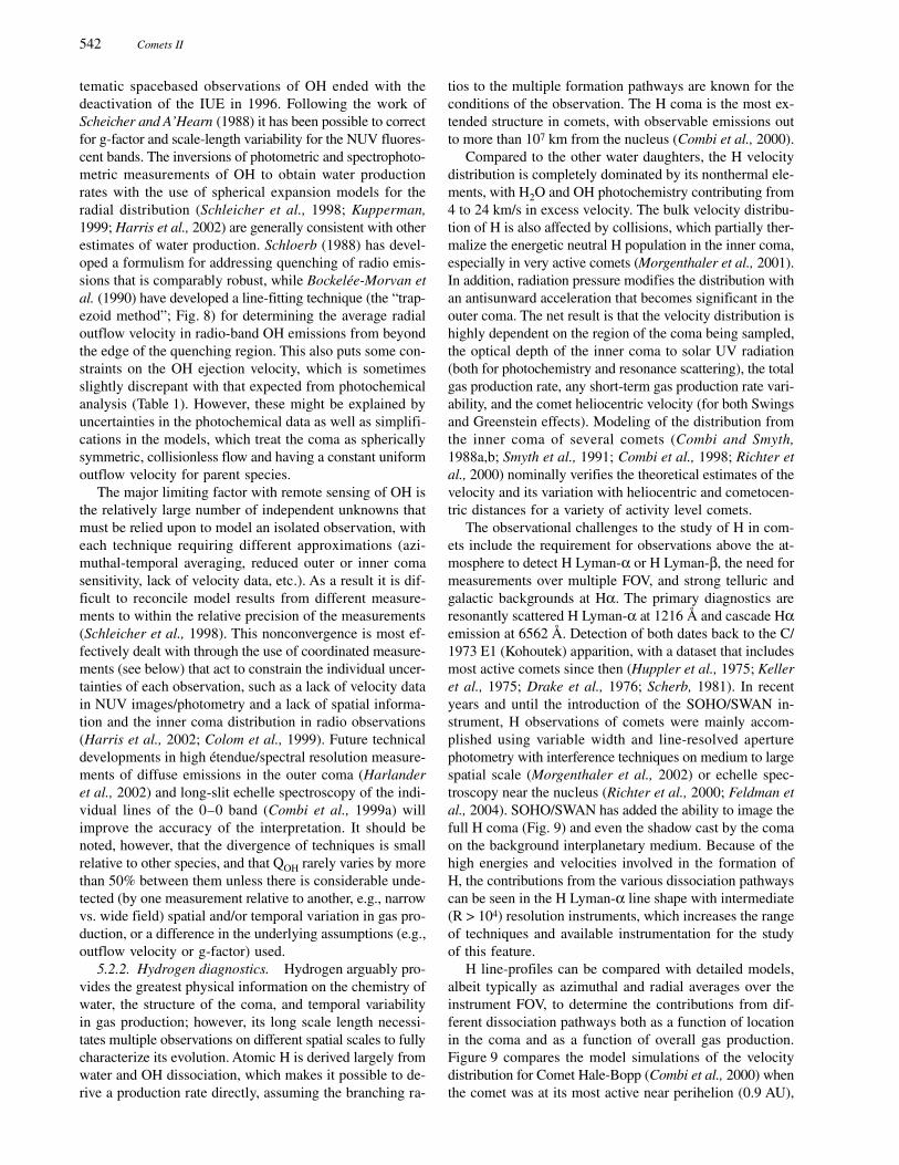
542 Comets II

tematic spacebased observations of OH ended with thedeactivation of the IUE in 1996. Following the work ofScheicher and A’Hearn (1988) it has been possible to correctfor g-factor and scale-length variability for the NUV fluores-cent bands. The inversions of photometric and spectrophoto-metric measurements of OH to obtain water productionrates with the use of spherical expansion models for theradial distribution (Schleicher et al., 1998; Kupperman,1999; Harris et al., 2002) are generally consistent with otherestimates of water production. Schloerb (1988) has devel-oped a formulism for addressing quenching of radio emis-sions that is comparably robust, while Bockelée-Morvan etal. (1990) have developed a line-fitting technique (the “trap-ezoid method”; Fig. 8) for determining the average radialoutflow velocity in radio-band OH emissions from beyondthe edge of the quenching region. This also puts some con-straints on the OH ejection velocity, which is sometimesslightly discrepant with that expected from photochemicalanalysis (Table 1). However, these might be explained byuncertainties in the photochemical data as well as simplifi-cations in the models, which treat the coma as sphericallysymmetric, collisionless flow and having a constant uniformoutflow velocity for parent species.

The major limiting factor with remote sensing of OH isthe relatively large number of independent unknowns thatmust be relied upon to model an isolated observation, witheach technique requiring different approximations (azi-muthal-temporal averaging, reduced outer or inner comasensitivity, lack of velocity data, etc.). As a result it is dif-ficult to reconcile model results from different measure-ments to within the relative precision of the measurements(Schleicher et al., 1998). This nonconvergence is most ef-fectively dealt with through the use of coordinated measure-ments (see below) that act to constrain the individual uncer-tainties of each observation, such as a lack of velocity datain NUV images/photometry and a lack of spatial informa-tion and the inner coma distribution in radio observations(Harris et al., 2002; Colom et al., 1999). Future technicaldevelopments in high étendue/spectral resolution measure-ments of diffuse emissions in the outer coma (Harlanderet al., 2002) and long-slit echelle spectroscopy of the indi-vidual lines of the 0–0 band (Combi et al., 1999a) willimprove the accuracy of the interpretation. It should benoted, however, that the divergence of techniques is smallrelative to other species, and that QOH rarely varies by morethan 50% between them unless there is considerable unde-tected (by one measurement relative to another, e.g., narrowvs. wide field) spatial and/or temporal variation in gas pro-duction, or a difference in the underlying assumptions (e.g.,outflow velocity or g-factor) used.

5.2.2. Hydrogen diagnostics. Hydrogen arguably pro-vides the greatest physical information on the chemistry ofwater, the structure of the coma, and temporal variabilityin gas production; however, its long scale length necessi-tates multiple observations on different spatial scales to fullycharacterize its evolution. Atomic H is derived largely fromwater and OH dissociation, which makes it possible to de-rive a production rate directly, assuming the branching ra-

tios to the multiple formation pathways are known for theconditions of the observation. The H coma is the most ex-tended structure in comets, with observable emissions outto more than 107 km from the nucleus (Combi et al., 2000).

Compared to the other water daughters, the H velocitydistribution is completely dominated by its nonthermal ele-ments, with H2O and OH photochemistry contributing from4 to 24 km/s in excess velocity. The bulk velocity distribu-tion of H is also affected by collisions, which partially ther-malize the energetic neutral H population in the inner coma,especially in very active comets (Morgenthaler et al., 2001).In addition, radiation pressure modifies the distribution withan antisunward acceleration that becomes significant in theouter coma. The net result is that the velocity distribution ishighly dependent on the region of the coma being sampled,the optical depth of the inner coma to solar UV radiation(both for photochemistry and resonance scattering), the totalgas production rate, any short-term gas production rate vari-ability, and the comet heliocentric velocity (for both Swingsand Greenstein effects). Modeling of the distribution fromthe inner coma of several comets (Combi and Smyth,1988a,b; Smyth et al., 1991; Combi et al., 1998; Richter etal., 2000) nominally verifies the theoretical estimates of thevelocity and its variation with heliocentric and cometocen-tric distances for a variety of activity level comets.

The observational challenges to the study of H in com-ets include the requirement for observations above the at-mosphere to detect H Lyman-α or H Lyman-β, the need formeasurements over multiple FOV, and strong telluric andgalactic backgrounds at Hα. The primary diagnostics areresonantly scattered H Lyman-α at 1216 Å and cascade Hαemission at 6562 Å. Detection of both dates back to the C/1973 E1 (Kohoutek) apparition, with a dataset that includesmost active comets since then (Huppler et al., 1975; Kelleret al., 1975; Drake et al., 1976; Scherb, 1981). In recentyears and until the introduction of the SOHO/SWAN in-strument, H observations of comets were mainly accom-plished using variable width and line-resolved aperturephotometry with interference techniques on medium to largespatial scale (Morgenthaler et al., 2002) or echelle spec-troscopy near the nucleus (Richter et al., 2000; Feldman etal., 2004). SOHO/SWAN has added the ability to image thefull H coma (Fig. 9) and even the shadow cast by the comaon the background interplanetary medium. Because of thehigh energies and velocities involved in the formation ofH, the contributions from the various dissociation pathwayscan be seen in the H Lyman-α line shape with intermediate(R > 104) resolution instruments, which increases the rangeof techniques and available instrumentation for the studyof this feature.

H line-profiles can be compared with detailed models,albeit typically as azimuthal and radial averages over theinstrument FOV, to determine the contributions from dif-ferent dissociation pathways both as a function of locationin the coma and as a function of overall gas production.Figure 9 compares the model simulations of the velocitydistribution for Comet Hale-Bopp (Combi et al., 2000) whenthe comet was at its most active near perihelion (0.9 AU),


and three months earlier (1.7 AU), when the production ratewas much lower and the dissociation rates much lower. Nearperihelion a large fraction of the highest-speed H atoms arethermalized to much lower velocities than at 1.7 AU wherethe distribution was not changed much. The effects of ther-malization are directly evident in the perihelion Hα line-profile measurements of Morgenthaler et al. (2002). Asdiscussed earlier, this slowing of the H atoms in Hale-Boppis matched by a corresponding increase in the outflow speedof the heavy species, to which the kinetic energy is beingtransferred. Both Harris et al. (2002) and Colom et al.(1999) see clear evidence of this effect in the velocity struc-ture of OH near Hale-Bopp’s perihelion. The shape of thecoma at perihelion, as shown in Fig. 9c and as observedwith the SWAN instrument on SOHO, is also sensitive tothe velocity distribution as first pointed out by Keller andMeier (1976).

The calculation of the water production rates (or anyspecies for that matter), from either fast species like H orslower heavier species like OH or water, is very sensitiveto our knowledge of the velocity distribution, unless the fullscale length is observed (see equation (26)). This compli-cation is substantially magnified by the multiple, radiallydependent components of the H velocity distribution andby the large spatial extent of the H coma. At present weare able to sample spectrally only small, discrete subsetsof the coma in the UV (H Lyman-α) or large azimuthallyand radially averaged areas at moderate signal to noise(Morgenthaler et al., 2002). Improvements in interferomet-ric instrument capabilities in the FUV (Stephan et al., 2001)and visible offer the promise of additional spatial informa-tion and increased spectral resolution for future comets.Other new diagnostics, including observations in the deepFUV (H Lyman-β) from FUSE (Feldman et al., 2002),measurements of Hβ emission from Comet C/1996 B2(Hyakutake) (Scherb et al., 1996), and the planned STE-REO (SOHO follow-up) mission, suggest a greater capa-bility to map the structure of the H coma in future comets.

5.2.3. O(1D) diagnostics. Oxygen in the metastable 1Dstate is a byproduct of H2O, OH, and CO photochemistrythat is produced at different rates across the coma. Relax-ation of O(1D) produces a single photon ~110 s after itsformation, meaning that its brightness inverts directly to itscombined parent production rate without any supplemen-tal knowledge of g-factors via equation (27) above. Onlythe various parent lifetimes and chemical branching ratiosare required to complete the inversion, and, if the full Ocoma is sampled, the lifetime dependence disappears aswell. Its short lifetime of the metastable state offers anadditional advantage, because the locations of formationand emission are nearly co-local. Thus, the radial distribu-tion of O(1D) is a radial map of the site of photochemistryin the coma that is useful for detailed modeling of chemi-cal rates, source distributions, and the relative density ratioof H2O and CO.

Observations of O(1D) do have significant complicationsas a proxy for H2O and OH photochemistry that are addres-sable to a large degree. Observationally, these complications

Fig. 9. Model for the SOHO SWAN observations of the HLyman-α coma of Comet 1995 O1 (Hale-Bopp); (a) and (b) showthe H-atom velocity distribution upon photochemical production(thin) and after Monte Carlo model calculation (thick) of thermal-ization in an expanding water-dominated coma. (a) Conditions onthe day of perihelion (April 1, 1997) when the comet was at aheliocentric distance of 0.91 AU and the water production rate was1.02 × 1031 s–1. (b) Conditions on January 1, 1997 when thesevalues were 1.75 AU and 2.2 × 1030 s–1 respectively. (c) Themodel-data comparison for the H coma at perihelion on April 1when collisional thermalization was the largest and the resultingcoma is the most distorted from spherical symmetry. The shapeof the coma is formed by the balance between solar radiationpressure acceleration and the velocity distribution function.

544 Comets II

include substantial telluric O(1D) nightglow, spectral sepa-ration of O I and nearby NH2 and H2O+ coma lines (seeFeldman et al., 2004), and the low contrast of the emissionover bright dust scattered continuum emission. Physicalcomplications include an unknown contribution from CO

photochemistry that can be partially correctable with obser-vations of C(1D) (see below) (Oliversen et al., 2002), un-certainty in the branching ratios from OH under differentlevels of solar activity (van Dishoeck et al., 1984; Huebneret al., 1992; Morgenthaler et al., 2001), UV opacity effectson chemical rates, and the role of collisional quenching andchemistry of O(1D) in the inner coma (Glinsky et al., 2003;Komitov, 1989). To compensate for the observational effects,O(1D) is now routinely observed using high-spectral-reso-lution (R > 15000) techniques including long-slit echellespectroscopy (Fink and Hicks, 1996), multiplexed echellespectroscopy (Fig. 10) (Anderson, 1999), interferometricdata cube imaging (Fig. 11), and aperture summed linemeasurements (Fig. 12). The recent detection of fluores-cence of metastable O I (D1-D1) by FUSE (Feldman et al.,2002) offers a potential new diagnostic that is comparableto the C(1D) line (see below).

As noted above, the integrated brightness of O(1D) isinvertable to a production rate with equation (27) and fromthere to QH2O from the branching ratios of OH and H2Ophotochemistry. The radial and azimuthal distribution of theemission traces both the expansion of the coma and the rateof collisional and chemical quenching in the inner coma.Because it maps directly to chemistry, O(1D) images alsoreveal extended sources and regions of increased velocity(Morgenthaler et al., 2002). The O(1D) outflow velocityretains the value of its parents (~1–2 km/s) plus fixed iso-tropic speed component of about 1.6 or 1.5 km/s from thephotochemical excess energy from H2O and OH, respec-tively. This requires high resolution (R < 105) to detect. Thiswas achieved for 1P/Halley in 1986, with a Fabry-Pérotinterferometer tuned to R = 1.9 × 105 (Fig. 12), although it

Fig. 10. Two types of multiport spectroscopy and their application to Comet Hale-Bopp are shown (from Morgenthaler et al., 2001).At left is a sample distribution using the Hydra spectrograph on the WIYN telescope. Here a set of 100 fibers are placed at pro-grammed positions over a 1° FOV with a minimum separation of 40 arcsec. The array design shown is optimized for the study ofradially distributed emission, with the individual fibers feeding a bench spectrograph mounted below the telescope pier. At center is aschematic of DensePak, a tight grouping of 100 fibers covering a region equal the minimum spacing in the Hydra array. At right is anexample of observation of O(1D) from Hale-Bopp using DensePak in the inner coma and Hydra for more remote locations.

Fig. 11. A single 1° field image slice of the O(1D) coma of Hale-Bopp is shown after subtraction of continuum. This image was ob-tained using the WHαM instrument at Kitt Peak (from Morgen-thaler et al., 2001). Overlaid is the location of fiber rings fromthe Hydra instrument using the array shown in Fig. 8.


required the averaging of a substantial FOV to obtain ac-ceptable s/n on the line-shape. The Halley profiles were fitsuccessfully using the Monte-Carlo particle trajectory modelof Combi et al. (1993) and were used to validate the model-predicted magnitude of expansion velocity and its increasewith increasing gas production (Smyth et al., 1995). Obser-vations of a similar resolution were made of the inner comaO(1D) distribution with a high-resolution echelle spectrom-eter of Comet C/1996 B2 (Hyakutake). These were also inagreement with model predictions for conditions interme-diate between the two Halley cases (Combi et al., 1999a).Continued development of very-high-resolution interfero-metric techniques and sensitive high-resolution echelle in-struments will make such observational programs routinefor comets of moderate to high activity, while the furtherdevelopment of FUSE band technology may provide a com-plementary diagnostic that will provide useful results forweaker comets.

5.2.4. Infrared and radio observations of H2O. A miss-ing key to the observational study of water dynamical andphotochemical evolution is measurement of the propertiesof the parent species. This has been historically difficult bothbecause of the lack of transitions in the FUV-visible bandand because of strong attenuation of IR and radio bandsby telluric water. Over the past two decades considerableprogress has been made in finding ways around the tellu-ric problem by moving to spacebased observatories or byobserving within the various windows where atmosphericabsorption is not so severe. Comets can sometimes be ob-served at large enough geocentric velocity in order to Dop-pler shift the cometary feature away from terrestrial absorp-tion features. These improvements offer considerable prom-ise that spacebased aperture photometry of water in theradio will become routine, while IR measurements (bothground- and spacebased) will contribute both the tempera-ture and radial distribution of water. Together they will fillan important observational niche in our study of coma ki-netics. The issue of observations of H2O, and parent mole-cules in general, is covered in detail in Bockelée-Morvanet al. (2004).

Unambiguous detection of water in the inner coma firstcame from 1P/Halley via the Kuiper Airborne Observatory(KAO) (Mumma et al., 1986) and the IKS instrument onthe Vega spacecraft (Combes et al., 1986), both of whichdirectly detected emission lines from the ν3 band near2.65 µm. In addition to providing a direct measurement ofH2O, the KAO data were used to derive both the nuclearspin temperature (Tspin) (Mumma et al., 1987) and the ro-tational temperature (Trot) (Bockelée-Morvan and Crovisier,1987) of the lines, which sample the formation history andthe current state of water in the coma respectively. The spintemperature derived from the ortho-para ratio on the dif-ferent detected lines of the ν3 band is set at the creation ofthe H2O molecule by either photochemistry or direct evapo-ration from ice on the nucleus and thus directly ties to thatevent. The results from 1P/Halley (Northo/Npara = 2.66 ± 0.13indicating Tspin = 32 K +5, –2) were consistent with the

Fig. 12. Aperture-summed O(1D) emission from 1P/Halley isdisplayed at the top showing the clean separation of comet andairglow O(1D) signatures from each other and cometary NH2

emission. These were obtained using a Fabry-Pérot interferom-eter in ring mode. Inspection of the comet and telluric line shapesshows the broadening in the Halley outflow. The lower panelsshow that this broadening is consistent with the magnitude ofcoma outflow predicted by model calculations to be broader atsmaller (middle panel) heliocentric distances and more narrow atlarger (bottom panel) distances (Smyth et al., 1995).

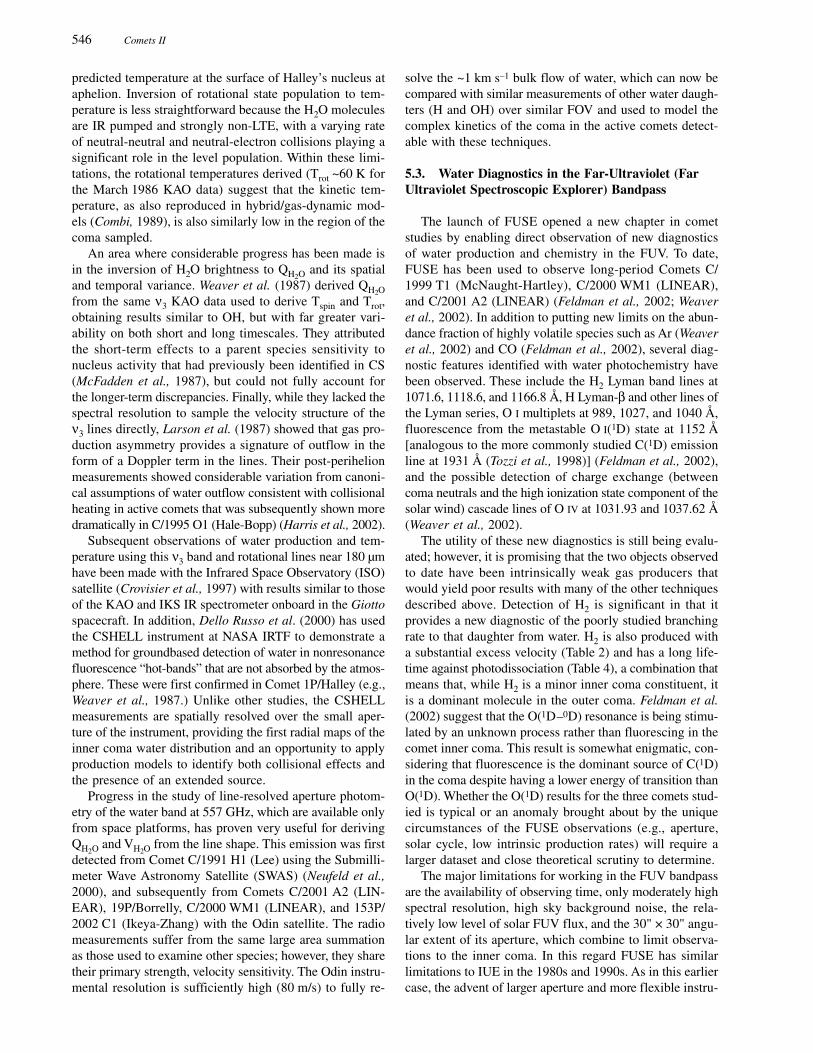
546 Comets II

predicted temperature at the surface of Halley’s nucleus ataphelion. Inversion of rotational state population to tem-perature is less straightforward because the H2O moleculesare IR pumped and strongly non-LTE, with a varying rateof neutral-neutral and neutral-electron collisions playing asignificant role in the level population. Within these limi-tations, the rotational temperatures derived (Trot ~60 K forthe March 1986 KAO data) suggest that the kinetic tem-perature, as also reproduced in hybrid/gas-dynamic mod-els (Combi, 1989), is also similarly low in the region of thecoma sampled.

An area where considerable progress has been made isin the inversion of H2O brightness to QH2O and its spatialand temporal variance. Weaver et al. (1987) derived QH2Ofrom the same ν3 KAO data used to derive Tspin and Trot,obtaining results similar to OH, but with far greater vari-ability on both short and long timescales. They attributedthe short-term effects to a parent species sensitivity tonucleus activity that had previously been identified in CS(McFadden et al., 1987), but could not fully account forthe longer-term discrepancies. Finally, while they lacked thespectral resolution to sample the velocity structure of theν3 lines directly, Larson et al. (1987) showed that gas pro-duction asymmetry provides a signature of outflow in theform of a Doppler term in the lines. Their post-perihelionmeasurements showed considerable variation from canoni-cal assumptions of water outflow consistent with collisionalheating in active comets that was subsequently shown moredramatically in C/1995 O1 (Hale-Bopp) (Harris et al., 2002).

Subsequent observations of water production and tem-perature using this ν3 band and rotational lines near 180 µmhave been made with the Infrared Space Observatory (ISO)satellite (Crovisier et al., 1997) with results similar to thoseof the KAO and IKS IR spectrometer onboard in the Giottospacecraft. In addition, Dello Russo et al. (2000) has usedthe CSHELL instrument at NASA IRTF to demonstrate amethod for groundbased detection of water in nonresonancefluorescence “hot-bands” that are not absorbed by the atmos-phere. These were first confirmed in Comet 1P/Halley (e.g.,Weaver et al., 1987.) Unlike other studies, the CSHELLmeasurements are spatially resolved over the small aper-ture of the instrument, providing the first radial maps of theinner coma water distribution and an opportunity to applyproduction models to identify both collisional effects andthe presence of an extended source.

Progress in the study of line-resolved aperture photom-etry of the water band at 557 GHz, which are available onlyfrom space platforms, has proven very useful for derivingQH2O and VH2O from the line shape. This emission was firstdetected from Comet C/1991 H1 (Lee) using the Submilli-meter Wave Astronomy Satellite (SWAS) (Neufeld et al.,2000), and subsequently from Comets C/2001 A2 (LIN-EAR), 19P/Borrelly, C/2000 WM1 (LINEAR), and 153P/2002 C1 (Ikeya-Zhang) with the Odin satellite. The radiomeasurements suffer from the same large area summationas those used to examine other species; however, they sharetheir primary strength, velocity sensitivity. The Odin instru-mental resolution is sufficiently high (80 m/s) to fully re-

solve the ~1 km s–1 bulk flow of water, which can now becompared with similar measurements of other water daugh-ters (H and OH) over similar FOV and used to model thecomplex kinetics of the coma in the active comets detect-able with these techniques.

5.3. Water Diagnostics in the Far-Ultraviolet (FarUltraviolet Spectroscopic Explorer) Bandpass

The launch of FUSE opened a new chapter in cometstudies by enabling direct observation of new diagnosticsof water production and chemistry in the FUV. To date,FUSE has been used to observe long-period Comets C/1999 T1 (McNaught-Hartley), C/2000 WM1 (LINEAR),and C/2001 A2 (LINEAR) (Feldman et al., 2002; Weaveret al., 2002). In addition to putting new limits on the abun-dance fraction of highly volatile species such as Ar (Weaveret al., 2002) and CO (Feldman et al., 2002), several diag-nostic features identified with water photochemistry havebeen observed. These include the H2 Lyman band lines at1071.6, 1118.6, and 1166.8 Å, H Lyman-β and other lines ofthe Lyman series, O I multiplets at 989, 1027, and 1040 Å,fluorescence from the metastable O I(1D) state at 1152 Å[analogous to the more commonly studied C(1D) emissionline at 1931 Å (Tozzi et al., 1998)] (Feldman et al., 2002),and the possible detection of charge exchange (betweencoma neutrals and the high ionization state component of thesolar wind) cascade lines of O IV at 1031.93 and 1037.62 Å(Weaver et al., 2002).

The utility of these new diagnostics is still being evalu-ated; however, it is promising that the two objects observedto date have been intrinsically weak gas producers thatwould yield poor results with many of the other techniquesdescribed above. Detection of H2 is significant in that itprovides a new diagnostic of the poorly studied branchingrate to that daughter from water. H2 is also produced witha substantial excess velocity (Table 2) and has a long life-time against photodissociation (Table 4), a combination thatmeans that, while H2 is a minor inner coma constituent, itis a dominant molecule in the outer coma. Feldman et al.(2002) suggest that the O(1D–0D) resonance is being stimu-lated by an unknown process rather than fluorescing in thecomet inner coma. This result is somewhat enigmatic, con-sidering that fluorescence is the dominant source of C(1D)in the coma despite having a lower energy of transition thanO(1D). Whether the O(1D) results for the three comets stud-ied is typical or an anomaly brought about by the uniquecircumstances of the FUSE observations (e.g., aperture,solar cycle, low intrinsic production rates) will require alarger dataset and close theoretical scrutiny to determine.

The major limitations for working in the FUV bandpassare the availability of observing time, only moderately highspectral resolution, high sky background noise, the rela-tively low level of solar FUV flux, and the 30" × 30" angu-lar extent of its aperture, which combine to limit observa-tions to the inner coma. In this regard FUSE has similarlimitations to IUE in the 1980s and 1990s. As in this earliercase, the advent of larger aperture and more flexible instru-


ments will improve our ability to monitor these importantnew features.

5.4. The Relationship of OtherComa Species to Water

Water is the dominant volatile component of comet nu-clei, and therefore its state and evolution are both relevantto developing an understanding of other coma species, someof which have reciprocal effects on the water coma. Theabove descriptions reveal several weaknesses in the diag-nostics suite used to determine the characteristics of thewater coma, and one technique to address this is to com-bine studies of water with other coma constituents that fillthese observational voids. The detailed physics of the othercoma species is dealt with in other chapters of this book,and our goal here is to illustrate only how a coordinatedobserving-modeling approach between them and water willincrease our understanding of each. While coordinatedobservations of multiple species provide benefits for under-standing many other properties of the coma, including itsthermal properties and the interaction of the solar wind, wewill briefly touch here on two examples (the velocity struc-ture of the inner coma and the role of secondary sourcesof water daughter species) where the above techniques pro-vide an incomplete picture and observational solutions us-ing other species have been identified.

5.4.1. Velocity structure. The low velocity of mostcoma constituents (in particular, H2O, OH, and O for water)requires extremely high spectral resolution (R > 105) tomeasure. Unfortunately, the most common technique used toachieve such high resolution in the visible and UV (echellespectroscopy) has a correspondingly small étendue thatsamples only small regions with fairly low sensitivity. Inter-ferometric techniques (Stephan et al., 2001; Watchorn et al.,2001; Morgenthaler et al., 2002) that co-add large FOV athigh spectral resolution in the visible and UV have consider-able future promise in this area; however, the most maturetechniques exist in the radio. Unfortunately, the primarywater diagnostic in the radio (OH at 18 cm) is stronglyquenched in the inner coma, which is its the most dynami-cally active region for active comets. To get around thisproblem it is possible to use other, less-quenched OH [e.g.,IR (Crovisier et al., 1997)] emission features or other spe-cies to study this region and combine the results to com-plete the dynamical picture. Several such features exist andare in common use to determine the velocity within ~103–104 km of the nucleus (Biver et al., 1999b). One commonlyobserved emission that is useful for such comparative workis the J = 1–0 line of HCN (Schloerb et al., 1987; Biver etal., 1999b), which is detectable close to the nucleus atsubkilometers per second velocity resolution and thereforeuseful in coordination with OH to measure velocity in theinner and outer coma. Models of the outflow (Combi, 1989)similar to those shown in Figs. 3–6 reproduced the secularvariation (with heliocentric distance) of the HCN line widthseen by Schloerb et al. (1987). Harris et al. (2002) com-bined published measurements of the outer coma OH ve-

locity (Colom et al., 1999) and inner coma HCN velocity(Biver et al., 1999a) with the radial distribution of emis-sion from OH to map out the acceleration across the comaof C/1995 O1 (Hale-Bopp). The magnitude and variationof these velocity measurements, both with distance fromthe nucleus and overall with heliocentric distance, are alsoin reasonable agreement with models for the expansion ofthe coma (Combi et al., 1999b), even for the extreme physi-cal state of Hale-Bopp.

5.4.2. Characterization secondary sources. Of the pri-mary neutral water species only H2O itself and OH haveno significant contribution from other sources. Of the oth-ers, O I has the largest nonwater component, in this casefrom a combination of CO and CO2. The precision of modelinterpretation of O(1D) will depend on the precision bywhich the CO- and H2O-derived components are separatedor by our knowledge of the CO/H2O ratio, which variessubstantially among comets and with heliocentric distance.The size of the CO/CO2 contribution can be dominant in theouter solar system, where water outgassing is suppressed,but even where water dominates, the addition of CO/CO2-derived O [particularly O(1D)] is significant. The role ofCO/CO2 is further complicated by the fact that the rate offormation of O(1D) differs between the two species and withrespect to both pathways in water. Indeed, O(1D), derivedfrom CO (as a daughter) and CO2 (as a granddaughter),most likely dominates over the OH contribution in the outercoma due to the longer lifetime of CO (Tozzi et al., 1998;Harris et al., 1999). This would be even further compli-cated by a substantial fraction of CO coming from an ex-tended source of another parent like H2CO (DiSanti et al.,2001). Moreover, the ratios of CO : CO2, CO/H2O, andCO2 : H2O vary substantially between comets, with no ob-vious predictive trend yet identified (Weaver et al., 1994;Feldman et al., 1997; see also Bockelée-Morvan et al.,2004). Thus, to account for the contribution of these spe-cies to the O(1D) brightness and spatial distribution, it isnecessary to study diagnostics of both CO and CO2 chem-istry. The most direct method is to study C(1D), the meta-stable analog to O(1D) that is formed in the same processfrom CO (Huebner et al., 1992; Tozzi et al., 1998). FromQ

C(1D) it is possible to separate the CO and OH contributions

directly over any simultaneously observed FOV.There are two diagnostics for C(1D): fluorescence from

the 1D state at 1931 Å and direct detection of the C(1D)decay at 9828/9850 Å. The former is accessible only fromspace and has typically been studied only over small FOV(Feldman et al., 1997), which limits its usefulness for a fullcoma correction. Direct observation of the NIR decay linesholds more promise, because it is both directly analogousto the O I visible line and observable from the ground. Thisfeature is faint compared to O(1D), has high backgroundcontamination, and falls near a telluric OH absorption. Ithas only been detected in two comets, first an unpublisheddetection from 1P/Halley by Münch et al. (1986), and morerecently from Fabry-Pérot interferometric observations ofC/1995 O1 Hale-Bopp (Oliversen et al., 2002). The Hale-Bopp detection provides the first quantitative estimates of

548 Comets II

the role of C(1D) in the inner and outer coma and identi-fies how future development of the interferometric tech-nique will improve our ability to study this diagnostic.

6. OUTSTANDING ISSUES AND FUTURESTUDIES OF COMA STRUCTURE

AND EXPANSION

There is currently no single diagnostic signature of wa-ter that provides a complete description of its spatial, ve-locity, temporal, and production rate evolution in the coma.Inferring such detail from any one observation thereforerequires either an estimate or approximation of the unknownquantities (usually from observed characteristics of earliercomets) or model derivation of them. As the quality of re-mote sensing data has improved, the limiting factor in in-terpretation has shifted from the instrumental regime to thedegree to which we know (1) underlying physical param-eters such as g-factors and rate constants; (2) internal fac-tors including quenching, temperature, solar wind densityand velocity, collision rates, optical depth, and source dis-tribution; (3) incoming solar spectral intensity in the UV;(4) parent species’ contributions and branching ratios; and(5) the two-dimensional and temporal structure of the comaand how it effects observations taken over different spatialscales or at different times.

To the extent that these parameters are known for eachcase, the modeling techniques discussed here each providea consistent picture of water evolution from the observa-tions. However, one effect of this shift is that the precisionof measurements now often greatly exceeds the accuracyof the inverted result (Schleicher et al., 1998). In many casesthe divergence between different methods stems more fromthe failure to fully account for this in the determination ofuncertainty than from the validity of the approach, and cangive the impression of nonconvergence when isolated ob-servations are compared directly. Another major effect isthe inversion or synthetic reproduction of data with spheri-cal and/or steady-state models. Not accounting for suchcomplicating effects can result in erroneously attributingfeatures in the data to those free parameters that are left inthe model. Finally, in the absence of simultaneous in situdata from multiple spacecraft, we are always left with theprojection of all information (spatial, velocity, and tempera-ture) along the line of sight that again can result in similarmisinterpretations.

A clear improvement of the model fits is obtained whenmultiple diagnostics with synergistic results and unknownsare combined, particularly if they are obtained nearly simul-taneously and can account for temporal and spatial vari-ances. For example, the combination of wide-field (produc-tion rate) and velocity-resolved (outflow and nonthermalcomponents) aperture photometry of a species with two-dimensional spatial imaging (parent-daughter scale lengths,azimuthal structure, propagating temporal activity changes)provides a set of reciprocal boundary values for the indi-vidual uncertainties in each observation. Where this ap-proach has been applied, it has significantly reduced the

allowed parameter space of the converged model for thecoma (Combi et al., 2000; Morgenthaler et al., 2001; Har-ris et al., 2002). The caveat to this is that the capability toperform the required observations is widely distributed andis typically organized only for high-profile apparitions (e.g.,1P/Halley, C/1995 O1 Hale-Bopp, C/1996 B2 Hyakutake).The results of these campaigns suggest that an improvementin our understanding of both the role of water in the comaand in the physical parameters that describe its evolutionwould result from a consistent organized effort targeting alarger sample of comets covering a wider range of activityand evolution.

Acknowledgments. M.R.C. acknowledges support from grantNAG5-13239 from the NASA Planetary Atmospheres program.

REFERENCES

A’Hearn M. F., Hoban S., Birch P. V., Bowers C., Martin R., andKlinglesmith D. A. III (1986) Cyanogen jets in Comet Halley.Nature, 324, 649–651.

Allen M., Delitsky M., Huntress W., Yung Y., and Ip W.-H. (1987)Evidence for methane and ammonia in the coma of Comet P/Halley. Astron. Astrophys., 187, 502–512.

Anderson C. M. (1999) Fiberoptically multiplexed medium resolu-tion spectroscopy from the WIYN telescope, singlet D neutraloxygen, NH2, and H2O+. Earth Moon Planets, 78, 99–104.

Bertaux J.-L. and Lallement R. (1984) Analysis of interplanetaryLyman-alpha line profile with a hydrogen absorption cell —Theory of the Doppler angular spectral scanning method.Astron. Astrophys., 140, 230–242.

Biver N., Bockelée-Morvan D., Colom P., Crovisier J., GermainB., Lellouch E., Davies J. K., Dent W. R. F., Moreno R.,Paubert G., Wink J., Despois D., Lis D. C., Mehringer D.,Benford D., Gardner M., Phillips T. G., Gunnarsson M.,Rickman H., Winnberg A., Bergman P., Johansson L. E. B.,and Rauer H. (1999a) Long-term evolution of the outgassingof Comet Hale-Bopp from radio observations. Earth MoonPlanets, 78, 5–11.

Biver N., Bockelée-Morvan D., Crovisier J., Davies J. K.,Matthews H. E., Wink J. E., Rauer H., Colom P., Dent W. R. F.,Despois D., Moreno R., Paubert G., Jewitt D., and Senay M.(1999b) Spectroscopic monitoring of Comet C/1996 B2 (Hya-kutake) with the JCMT and IRAM radio telescopes. Astron. J.,118, 1850–1872.

Biver N., Bockelée-Morvan D., Colom P., Crovsier J., Henry F.,Lellouch E., Winnberg A., Johansson L. E. B., Cunnarsson M.,Rickman H., Rantakyrö F., Davies J. K., Dent W. R. F., PaubertG., Moreno R., Wink J., Despois D., Benford D. J., Gardner M.,Lis D. C., Mehringer D., Phillips T. G., and Rauer H. (2002)The 1995–2002 long-term monitoring of Comet C/1995 O1(Hale-Bopp) at radio wavelength. Earth Moon Planets, 90, 5–14.

Bird G. A. (1994) Molecular Gas Dynamics and the Direct Simu-lation of Gas Flows. Clarendon, Oxford. 459 pp.

Bockelée-Morvan D. (1987) A model for the excitation of water incomets. Astron. Astrophys., 181, 169–181.

Bockelée-Morvan D. and Crovisier J. (1987) The role of water inthe thermal balance of the coma. In Proceedings of the Sym-posium on the Diversity and Similarity of Comets (E. J. Rolfeand B. Battrick, eds.), pp. 235–240. ESA SP-278, Noordwijk,The Netherlands.


Bockelée-Morvan D., Crovisier J., and Gerard E. (1990) Retriev-ing the coma gas expansion velocity in P/Halley, Wilson(1987 VII) and several other comets from the 18-cm OH lineshapes. Astron. Astrophys., 238, 382–400.

Bockelée-Morvan D., Crovisier J., Colom P., and Despois D.(1994) The rotational lines of methanol in Comets Austin1990 V and Levy 1990 XX. Astron. Astrophys., 287, 647–665.

Bockelée-Morvan D., Crovisier J., Mumma M. J., and WeaverH. A. (2004) The composition of cometary volatiles. In Com-ets II (M. C. Festou et al., eds.), this volume. Univ. of Arizona,Tucson.

Brooke T. Y., Tokunaga A. T., Weaver H. A., Crovisier J.,Bockelée-Morvan D., and Crisp D. (1996) Detection of acety-lene in the infrared spectrum of Comet Hyakutake. Nature, 383,606–608.

Brooke T. Y., Weaver H. A., Chin G., Bockelée-Morvan D., KimS. J., and Xu L.-H. (2003) Spectroscopy of Comet Hale-Boppin the infrared. Icarus, 166, 167–187.

Budzien S. A., Festou M. C., and Feldman P. D. (1994) Solar fluxvariability of cometary H2O and OH. Icarus, 107, 164–188.

Chin G. and Weaver H. A. (1984) Vibrational and rotational exci-tation of CO in comets. Nonequilibrium calculations. Astro-phys. J., 285, 858–869.

Cochran A. L. (1985) A re-evaluation of the Haser model scalelengths for comets. Astron. J., 90, 2609–2514.

Cochran A. L. and Schleicher D. G. (1993) Observational con-straints on the lifetime of cometary H2O. Icarus, 105, 235–253.

Colom P., Gerard E., Crovisier J., Bockelée-Morvan D., Biver N.and Rauer H. (1999) Observations of the OH radical in CometC/1995 O1 (Hale-Bopp) with the Nançay radio telescope.Earth Moon Planets, 78, 37–43.

Combes M., Moroz V., Crifo J.-F., Lamarre J. M., Charra J., SankoN. F., Soufflot A., Bibring J. P., Cazes S., Coron N., CrovisierJ., Emerich C., Encrenaz T., Gispert R., Grigoryev A. V., GuyotG., Krasnopolsky V. A., Nikolsky Yu. V., and Rocard F. (1986)Infrared sounding of Comet Halley from Vega 1. Nature, 321,266–268.

Combi M. R. (1987) Sources of cometary radicals and their jets —Gases or grains. Icarus, 71, 178–191.

Combi M. R. (1989) The outflow speed of the coma of Halley’scomet. Icarus, 81, 41–50.

Combi M. R. (1996) Time-dependent gas kinetics in tenuous plan-etary atmospheres: The cometary coma. Icarus, 123, 207–226.

Combi M. R. (2002) Hale-Bopp: What makes a big comet differ-ent. Coma dynamics: Observations and theory. Earth MoonPlanets, 89, 73–90.

Combi M. R. and Delsemme A. H. (1980) Neutral cometaryatmospheres. I. Average random walk model for dissociationin comets. Astrophys. J., 237, 633–641.

Combi M. R. and Fink U. (1993) P/Halley — Effects of time-dependent production rates on spatial emission profiles. Astro-phys. J., 409, 790–797.

Combi M. R. and Fink U. (1997) A critical study of molecularphotodissociation and CHON grain sources for cometary C.Astrophys. J., 484, 879–890.

Combi M. R. and Smyth W. H. (1988a) Monte Carlo particle tra-jectory models for neutral cometary gases. I. Models and equa-tions. Astrophys. J., 327, 1026–1043.

Combi M. R. and Smyth W. H. (1988b) Monte Carlo particle tra-jectory models for neutral cometary gases. II. The spatialmorphology of the Lyman-alpha coma. Astrophys. J., 327,1044–1059.

Combi M. R., Bos B. J., and Smyth W. H. (1993) The OH distri-bution in cometary atmospheres — A collisional Monte Carlomodel for heavy species. Astrophys. J., 408, 668–677.

Combi M. R., Brown M. E., Feldman P. D., Keller H. U., MeierR. R., and Smyth W. H. (1998) Hubble Space Telescope ul-traviolet imaging and high-resolution spectroscopy of waterphotodissociation products in Comet Hyakutake (C/1996 B2).Astrophys. J., 494, 816–821.

Combi M. R., Cochran A. L., Cochran W. D., Lambert D. L., andJohns-Krull C. M. (1999a) Observation and analysis of high-resolution optical line profiles in Comet Hyakutake (C/1996B2). Astrophys. J., 512, 961–968.

Combi M. R., Kabin K., DeZeeuw D. L., Gombosi T. I., andPowell K. G. (1999b) Dust-gas interrelations in comets: Obser-vations and theory. Earth Moon Planets, 79, 275–306.

Combi M. R., Reinard A. A., Bertaux J.-L., Quemerais E., andMäkinen T. (2000) SOHO/SWAN observations of the structureand evolution of the hydrogen Lyman-alpha: Coma of CometHale-Bopp (1995 O1). Icarus, 144, 191–202.

Cravens T. E., Kozyra J. U., Nagy A. F., Gombosi T. I., and KurtzM. (1987) Electron impact ionization in the vicinity of comets.J. Geophys. Res., 92, 7341–7353.

Crifo J.-F., Crovisier J., and Bockelée-Morvan D. (1989) Proposedwater velocity and temperature radial profiles appropriate tocomet Halley flyby conditions. Paper presented at the 121stColloquium of the International Astronomical Union, held inBamberg, Germany, April 24–28, 1989.

Crifo J.-F., Itkin A. L., and Rodionov A. V. (1995) The near-nucleus coma formed by interacting dusty gas jets effusingfrom a cometary nucleus: I. Icarus, 116, 77–112.

Crifo J.-F., Rodionov A. V., and Bockelée-Morvan D. (1999) Thedependence of the circumnuclear coma structure on the prop-erties of the nucleus. Icarus, 138, 85–106.

Crifo J.-F., Lukianov G. A., Rodionov A.V., Khanlarov G. O., andZakharov V. V. (2002) Comparison between Navier-Stokes anddirect Monte-Carlo simulations of the circumnuclear coma.I. Homogeneous, spherical source. Icarus, 156, 249–268.

Crifo J.-F., Loukianov G. A., Rodionov A. V., and Zakharov V. V.(2003) Navier-Stokes and direct Monte Carlo simulations ofthe circumnuclear coma II. Homogeneous, aspherical sources.Icarus, 163, 479–503.

Crifo J.-F., Kömle N. I., Fulle M., and Szegö K. (2004) Nucleus-coma structural relationships: Lessons from physical models.In Comets II (M. C. Festou et al., eds.), this volume. Univ. ofArizona, Tucson.

Crovisier J. (1984) The water molecule in comets: Fluorescencemechanisms and thermodynamics of the inner coma. Astron.Astrophys., 130, 361–372.

Crovisier J. (1989) The photodissociation of water in cometaryatmospheres. Astron. Astrophys., 213, 459–464.

Crovisier J., Leech K., Bockelée-Morvan D., Brooke T. Y., HannerM. S., Altieri B., Keller H. U., and Lellouch E. (1997) Thespectrum of Comet Hale-Bopp (C/1995 O1) observed with theinfrared space observatory at 2.9 astronomical units from theSun. Science, 275, 1904–1907.

Crovisier J., Colom P., Gérard E., Bockelée-Morvan D., andBourgois G. (2002) Observations at Nançay of the OH 18-cmlines in comets. The data base. Observations made from 1982to 1999. Astron. Astrophys., 393, 1053–1064.

Dello Russo N., Mumma M. J., DiSanti M. A., Magee-Sauer K.,Novak R., and Rettig T. W. (2000) Water production and re-lease in Comet C/1995 O1 Hale-Bopp. Icarus, 143, 324–337.

Delsemme A. H. and Miller D. C. (1971) The continuum of Comet

550 Comets II

Burnham (1960 II): The differentiation of a short period comet.Planet. Space Sci., 19, 1229–1257.

DiSanti M. A., Mumma M. J., Dello Russo N., and Magee-SauerK. (2001) Carbon monoxide production and excitation inComet C/1995 O1 (Hale-Bopp): Isolation of native and dis-tributed CO sources. Icarus, 153, 162–179.

Drake J. F., Jenkins E. B., Bertaux J.-L., Festou M., and KellerH. U. (1976) Lyman-alpha observations of Comet Kohoutek1973 XII with Copernicus. Astrophys. J., 209, 302–311.

Eberhardt P., Krankowsky D., Schulte W. , Dolder U., LämmerzahlP., Berthelier J. J., Woweries J., Stubbeman U., Hodges R. R.,Hoffman J. H., and Illiano J. M. (1987) The CO and N2 abun-dance in Comet P/Halley. Astron. Astrophys., 187, 481–484.

Eddington A. S. (1910) The envelopes of c 1908 (Morehouse).Mon. Not. R. Astron. Soc., 70, 442–458.

Fahr H. J. and Shizgal B. (1981) Modern exospheric theories andtheir observational relevance. Rev. Geophys., 21, 75–124.

Farnham T. L., Schleicher D. G., and A’Hearn M. F. (2000) TheHB narrowband comet filters: Standard stars and calibrations.Icarus, 147, 180–204.

Feldman P. D., Festou M. C., Tozzi G. P., and Weaver H. A. (1997)The CO2/CO abundance ratio in 1P/Halley and several othercomets observed by IUE and HST. Astrophys. J., 475, 829–834.

Feldman P. D., Weaver H. A., and Burgh E. B. (2002) Far Ultra-violet Spectroscopic Explorer observations of CO and H2 emis-sion in Comet C/2001 A2 (LINEAR). Astrophys. J. Lett., 576,L91–L94.

Feldman P. D., Cochran A. L., and Combi M. R. (2004) Spectro-scopic investigations of fragment species in the coma. In Com-ets II (M. C. Festou et al., eds.), this volume. Univ. of Arizona,Tucson.

Festou M. C. (1981a) The density distribution of neutral com-pounds in cometary atmospheres. I — Models and equations.Astron. Astrophys., 95, 69–79.

Festou M. C. (1981b) The density distribution of neutral com-pounds in cometary atmospheres. II — Production rate andlifetime of OH radicals in Comet Kobayashi-Berger-Milon/1975 IX/. Astron. Astrophys., 96, 52–57.

Festou M. C. (1999) On the existence of distributed sources incomet comae. Space Sci. Rev., 90, 53–67.

Festou M. C. and Feldman P. D. (1981) The forbidden oxygenlines in comets. Astron. Astrophys., 103, 154–159.

Fink U. and Hicks M. D. (1996). A survey of 39 comets usingCCD spectroscopy. Astrophys. J., 459, 729–743.

Fink U., Combi M. R., and DiSanti M. A. (1991) Comet P/Halley — Spatial distributions and scale lengths for C2, CN,NH2, and H2O. Astrophys. J., 383, 356–371.

Finson M. L. and Probstein R. F. (1968) A theory of dust comets.1. Model and equations. Astrophys. J., 154, 327–352.

Fokker A. D. (1953) Some notes on the fountain model of com-etary envelopes and streamers. Mem. Sci. Liége, Ser. 4, 13,241–259.

Glinski R. J., Harris W. M., Anderson C. M., and MorgenthalerJ. P. (2003) Oxygen/hydrogen chemistry in inner comae ofactive comets. In Formation of Cometary Material, 25th Meet-ing of the IAU, Joint Discussion 14, 22 July 2003, Sydney,Australia.

Gombosi T. I. (1994) Gaskinetic Theory. Cambridge Univ., Cam-bridge. 297 pp.

Gombosi T. I., Cravens T. E., and Nagy A. F. (1985) Time-de-pendent dusty gas dynamical flow near cometary nuclei. Astro-phys. J., 293, 328–341.

Gombosi T. I., Nagy A. F., and T. E. Cravens (1986) Dust andneutral gas modeling of the inner atmospheres of comets. Rev.Geophys., 24, 667–700.

Grün E., Hanner M. S., Peschke S. B., Müller T., Boehnhardt H.,Brooke T. Y., Campins H., Crovisier J., Delahodde C., Hein-richsen I., Keller H. U., Knacke R. F., Krüger H., Lamy P.,Leinert C., Lemke D., Lisse C. M., Müller M., Osip D. J., SolcM., Stickel M., Sykes M., Vanysek V., and Zarnecki J. (2001)Broadband infrared photometry of Comet Hale-Bopp withISOPHOT. Astron. Astrophys., 377, 1098–1118.

Häberli R., Combi M. R., Gombosi T. I., De Zeeuw D. L., andPowell K. G. (1997) Quantitative analysis of H2O+ coma im-ages using a multiscale MHD model with detailed ion chem-istry. Icarus, 130, 373–386.

Harlander J. M., Roesler F. L., Cardon J. G., Englert C. R., andConway R. R. (2002) Shimmer: A spatial heterodyne spec-trometer for remote sensing of Earth’s middle atmosphere.Applied Optics, 41, 1343–1352.

Harmon J. K., Ostro S. J., Benner L. A. M., Rosema K. D., JurgensR. F., Winkler R., Yeomans D. K., Choate D., Cormier R.,Giogini J. D., Mitchell D. L., Chodas P. W., Rose R., KelleyD., Slade M. A., and Thomas M. L. (1997) Radar detectionof the nucleus and coma of Comet Hyakutake (C/1996 B2).Science, 278, 1921–1924.

Harris W. M., Combi M. R., Honeycutt R. K., and MuellerB. E. A. (1997) Evidence for interacting gas flows and anextended volatile source distribution in the coma of Comet C/1996 B2 (Hyakutake). Science, 277, 676–681.

Harris W. M., Nordsieck K. H., Scherb F., and Mierkiewicz E. J.(1999) UV photopolarimetric imaging of C/1995 O1 (Hale-Bopp) with the Wide Field Imaging Survey Polarimeter(WISP). Earth Moon Planets, 78, 161–167.

Harris W. M., Scherb F., Mierkiewicz E. J., Oliversen R. J., andMorgenthaler J. P. (2002) Production, outflow velocity, andradial distribution of H2O and OH in the coma of Comet C/1995 O1 [Hale-Bopp] from wide field imaging of OH. Astro-phys. J., 578, 996–1008.

Haser L. (1957) Distribution d’intensite dans la tete d’une comete.Bull. Acad. R. de Belgique, Classe de Sci. 43(5), 740–750.

Hodges R. R. (1990) Monte Carlo simulation of nonadiabaticexpansion in cometary atmospheres: Halley. Icarus, 83, 410–433.

Huebner W. F. (1985) The photochemistry of comets. In ThePhotochemistry of Atmospheres: Earth, the Other Planets, andComets (J. S. Levine, ed.), pp. 437–481. Academic, Orlando.

Huebner W. F. and Carpenter C. W. (1979) Solar Photo RateCoefficients. Los Alamos Sci. Lab. Report LA-8085-MS, LosAlamos National Laboratory, Los Alamos, New Mexico.

Huebner W. F. and Keady J. J. (1983) Energy balance and photo-chemical processes in the inner coma. In Cometary Explora-tion, Vol. 1 (T. I. Gombosi, ed.), pp. 165–183. Central ResearchInstitute for Physics, Budapest, Hungary.

Huebner W. F., Keady J. J., and Lyon S. P. (1992) Solar photo ratesfor planetary atmospheres and atmospheric pollutant. Astro-phys. Space Sci., 195, 1–294.

Huppler D., Reynolds R. J., Roesler F. L., Scherb F., and TraugerJ. (1975) Observations of Comet Kohoutek /1973f/ with aground-based Fabry-Pérot spectrometer. Astrophys. J., 202,276–282.

Ip W.-H. (1983) On photochemical heating of cometary comae:The cases of H2O and CO-rich comets. Astrophys. J., 264,726–732.

Ip W.-H. (1989) Photochemical heating of cometary comae.


III. The radial variation of the expansion velocity of CN shellsin comet Halley. Astrophys. J., 346, 475–480.

Jackson W. M. (1976) Laboratory observations of the photochem-istry of parent molecules: A review. In The Study of Comets(B. Donn et al., eds.), pp. 679–704. NASA SP-393, Washing-ton, DC.

Jackson W. M. (1980) The lifetime of the OH radical in cometsat 1 AU. Icarus, 41, 147–152.

Jewitt D., Senay M., and Matthews H. (1996) Observations of car-bon monoxide in Comet Hale-Bopp. Science, 271, 1110–1113.

Kawakita H. and Watanabe J. (1998) NH2 and its parent moleculein the inner coma of Comet Hyakutake (C/1996 B2). Astrophys.J., 495, 946–950.

Kawakita H., Watanabe J., Ando H., Alki W., Fuse T., Honda S.,Izumiura H., Kajino T., Kambe E., Kawanaomoto S., NoguchiK., Okita K., Sadakane K., Sato B., Takada-Midai M., TakedaY., Usunda T., Watanabe E., and Yoshinda M. (2001) The spintemperature of NH3 in Comet C/1994 S4 (LINEAR). Science,294, 1089–1091.

Keller H. U. and Meier R. R. (1976) A cometary hydrogen modelfor arbitrary observational geometry. Astron. Astrophys., 52,273–281.

Keller H. U., Bohlin J. D., and Tousey R. (1975) High resolutionLyman alpha observations of Comet Kohoutek /1973f/ nearperihelion. Astron. Astrophys., 38, 413–416.

Kiselev N. N. and Velichko F. P. (1999) Aperture polarimetry andphotometry of Comet Hale-Bopp. Earth Moon Planets, 78,347–352.

Kitamura Y. (1986) Axisymmetric dusty gas jet in the inner comaof a comet. Icarus, 66, 241–257.

Kitamura Y., Ashihara O., and Yamamoto T. (1985) A model forthe hydrogen coma of a comet. Icarus, 61, 278–295.

Komitov B. (1989) The metastable oxygen O (1D) as a possiblesource of OH molecules in the cometary atmospheres. Adv.Space Res., 9, 177–179.

Körösmezey A. and Gombosi T. I. (1990) A time-dependent dustygas dynamic model of axisymmetric cometary jets. Icarus, 84,118–153.

Krasnopolsky V. A. and 34 colleagues (1986a) The VEGA-2 TKSexperiment — Some spectroscopic results for Comet Halley.Soviet Astron. Lett., 12(4), 259–262.

Krasnopolsky V. A. and 13 colleagues (1986b) Spectroscopicstudy of Comet Halley by the VEGA 2 three-channel spectrom-eter. Nature, 321, 269–271.

Kupperman D. G. (1999) Nonthermal atoms in planetary, satellite,and cometary atmospheres. Ph.D. thesis, The Johns HopkinsUniversity, Baltimore, Maryland.

Lämmerzahl P. and 11 colleagues (1987) Expansion velocity andtemperatures of gas and ions measured in the coma of CometP/Halley. Astron. Astrophys., 187, 169–173.

Lamy P. L. and Perrin J.-M. (1988) Optical properties of organicgrains — Implications for interplanetary and cometary dust.Icarus, 76, 100–109.

Larson H. P., Mumma M. J., and Weaver H. A. (1987) Kinematicproperties of the neutral gas outflow from Comet P/Halley.Astron. Astrophys., 187, 391–397.

Lecacheux, A., Biver N., Crovisier J., Bockelée-Morvan D., BaronP., Booth R. S., Encrenaz P., Florén H.-G., Frisk U., Hjalmar-son Å., Kwok S., Mattila K., Nordh L, Olberg M., OlofssonA. O. H., Rickman H., Sandqvist Aa., von Schéele F., SerraG., Torchinsky S., Volk K., and Winnberg A. (2003) Observa-tions of water in comets with Odin. Astron. Astrophys., 402,L55–L58.

Marconi M. L. and Mendis D. A. (1983) The atmosphere of adirty-clathrate cometary nucleus — two-phase, multifluidmodel. Astrophys. J., 273, 381–396.

Markiewicz W. J., Skorov Y. V., Keller H. U., and Kömle N. I.(1998) Evolution of ice surfaces within porous near-surfacelayers on cometary nuclei. Planet. Space Sci., 46, 357–366.

McFadden L. A., A’Hearn M. F., Edsall D. M., Feldman P. D.,Roettger E. E., and Butterworth P. S. (1987) Activity of CometP/Halley 23–25 March, 1986 — IUE observations. Astron.Astrophys., 187, 333–338.

Meier R., Eberhardt P., Krankowsky D., and Hodges R. R. (1993)The extended formaldehyde source in Comet P/Halley. Astron.Astrophys., 277, 677–690.

Mocknatsche D. O. (1938) Leningrad State Univ. Annals, Astron.Series Issue 4.

Morgenthaler J. P., Harris W. M., Scherb F., Anderson C. M.,Oliversen R. J., Doane N. E., Combi M. R., Marconi M. L.,and Smyth W. H. (2001) Large-aperture [O I] 6300 Å photom-etry of Comet Hale-Bopp: Implications for the photochemistryof OH. Astrophys. J., 563, 451–461.

Morgenthaler J. P., Harris W. M., Scherb F., and Doane N. E.(2002) Velocity resolved observations of H-α emission fromComet Hale-Bopp. Earth Moon Planets, 90, 77–87.

Mumma M. J., Weaver H. A., Larson H. P., Davis D. S., andWilliams M. (1986) Detection of water vapor in Halley’scomet. Science, 232, 1523–1528.

Mumma M. J., Weaver H. A., and Larson H. P. (1987) The ortho-para ratio of water vapor in Comet P/Halley. Astron. Astrophys.,187, 419–424.

Mumma M. J., McLean I. S., DiSanti M. A., Larkin J. E., DelloRusso N., Magee-Sauer K., Becklin E. E., Bida T., Chaffee F.,Conrad A. R., Figer D. F., Gilbert A. M., Graham J. R.,Levenson N. A., Novak R. E., Reuter D. C., Teplitz H. I.,Wilcox M. I., and Li-Hong X. (2001) A survey of organicvolatile species in Comet C/1999 H1 (Lee) using NIRSPEC atthe Keck Observatory. Astrophys. J., 546, 1183–1193.

Münch G., Hippelein H., Hessmann F., and Gredel R. (1986)Periodic Comet Halley (1982i). IAU Circular No. 4183.

Nee J. B. and Lee L. C. (1985) Photodissociation rates of OH,OD, and CN by the interstellar radiation field. Astrophys. J.,291, 202–206.

Neufeld D. A., Stauffer J. R., Bergin E. A., Kleiner S. C., PattenB. M., Wang Z., Ashby M. L. N., Chin G., Erickson N. R.,Goldsmith P. F., Harwit M., Howe J. E., Koch D. G., PlumeR., Schieder R., Snell R. L., Tolls V., Winnewisser G., ZhangY. F., and Melnick G. J. (2000) Submillimeter wave astronomysatellite observations of water vapor toward Comet C/1999 H1(Lee). Astrophys. J. Lett., 539, L151–L154.

O’Dell C. R., Robinson R. R., Krishna Swamy K. S., McCarthyP. J., and Spinrad H. (1988) C2 in Comet Halley: Evidence forits being third generation and resolution of the vibrational pop-ulation discrepancy. Astrophys. J., 334, 476–488.

Oliversen R. J., Doane N. E., Scherb F., Harris W. M., andMorgenthaler J. P. (2002) Measurements of C I emission fromComet Hale-Bopp. Astrophys. J., 581, 770–775.

Oppenheimer M. and Downey C. J. (1980) The effect of solar-cycle ultraviolet flux variations on cometary gas. Astrophys.J. Lett., 241, L123–L127.

Prialnik D., Benkhoff J., and Podolak M. (2004) Modeling thestructure and activity of comet nuclei. In Comets II (M. C.Festou et al., eds.), this volume. Univ. of Arizona, Tucson.

Richter K., Combi M. R., Keller H. U., and Meier R. R. (2000)Multiple scattering of Hydrogen Ly-alpha: Radiation in the

552 Comets II

coma of Comet Hyakutake (C/1996 B2). Astrophys. J., 531,599–611.

Rodgers S. D., Charnley S. B., Huebner W. F., and Boice D. C.(2004) Physical processes and chemical reactions in cometarycomae. In Comets II (M. C. Festou et al., eds.), this volume.Univ. of Arizona, Tucson.

Scherb F. (1981) Hydrogen production rates from ground-basedFabry-Pérot observations of Comet Kohoutek. Astrophys. J.,243, 644–650.

Scherb F., Roesler F. L., Tufte S., and Haffner M. (1996) Fabry-Pérot observations of [O I] 6300, Hα, Hβ and NH2 emissionsfrom Comet Hyakutake C/1996 B2. Bull. Am. Astron. Soc., 28,927.

Schleicher D. G. and A’Hearn M. F. (1982) OH fluorescence incomets — Fluorescence efficiency of the ultraviolet bands.Astrophys. J., 258, 864–877.

Schleicher D. G. and A’Hearn M. F. (1988) The fluorescence ofcometary OH. Astrophys. J., 331, 1058–1077.

Schleicher D. G. and Farnham T. L. (2004) Photometry and im-aging of the coma with narrowband filters. In Comets II (M. C.Festou et al., eds.), this volume. Univ. of Arizona, Tucson.

Schleicher D. G., Millis R. L., Thompson D. T., Birch P. V., MartinR. M., Tholen D. J., Piscitelli J. R., Lark N. L., and HammelH. B. (1990) Periodic variations in the activity of Comet P/Halley during the 1985/1986 apparition. Astron. J., 100, 896–912.

Schleicher D. G., Millis R. L., and Birch P. V. (1998) Narrowbandphotometry of Comet P/Halley: Variation with heliocentric dis-tance, season, and solar phase angle. Icarus, 132, 397–417.

Schloerb F. P. (1988) Collisional quenching of cometary emissionin the 18 centimeter OH transitions. Astrophys. J., 332, 524–530.

Schloerb F. P., Kinzel W. M., Swade D. H., and Irvine W. M.(1987) Observations of HCN in Comet P/Halley. Astron. Astro-phys., 187, 475–480.

Schloerb F. P., Devries C. H., Lovell A. J., Irvine W. M., SenayM., and Wootten H. A. (1999) Collisional quenching of OHradio emission from Comet Hale-Bopp. Earth Moon Planets,78, 45–51.

Schultz D., Li G. S. H., Scherb F., and Roesler F. L. (1993) TheO(1D) distribution of Comet Austin 1989c1 = 1990 V. Icarus,101, 95–107.

Shimizu M. (1976) The structure of cometary atmospheres. Astro-phys. Space Sci., 40, 149–155.

Skorov Y. V. and Rickman H. (1999) Gas flow and dust accelera-tion in a cometary Knudsen layer. Planet. Space Sci., 47, 935–949.

Skorov Y., Kömle N. I., Keller H. U., Kargle G., and MarkiewiczW. J. (2001) A model of heat and mass transfer in a porouscometary nucleus based on a kinetic treatment of mass flow.Icarus, 153, 180–196.

Slanger T. G and Black G. (1982) Photodissociation channels at1216 Å for H2O, NH3, and CH4. J. Chem. Phys., 77, 2432–2437.

Smyth W. H., Combi M. R., and Stewart A. I. F. (1991) Analysisof the Pioneer Venus Lyman-α image of the hydrogen comaof Comet P/Halley. Science, 253, 1008–1010.

Smyth W. H., Combi M. R., Roesler F. L., and Scherb F. (1995)Observations and analysis of O(1D) and NH2 line profiles forthe coma of Comet P/Halley. Astrophys. J., 440, 349–360.

Stephan S. G., Chakrabarti S., Vickers J., Cook T., and Cotton D.(2001) Interplanetary H Ly-α: Observations from a soundingrocket. Astrophys. J., 559, 491–500.

Stief L. J., Payne W. A., and Klemm R. B. (1975) A flash pho-tolysis-resonance fluoresccnce study of the formation of O(1D)in the photolysis of water and the reaction of O(1D) with H2,Ar, and He. J. Chem. Phys., 62, 4000–4008.

Tegler S. C., Burke L. F., Wyckoff S., Womack M., Fink U., andDiSanti M. (1992) NH3 and NH2 in the coma of CometBrorsen-Metcalf. Astrophys. J., 384, 292–297.

Tozzi G. P., Feldman P. D., and Festou M. C. (1998) Origin andproduction of C(1D) atoms in cometary comae. Astron. Astro-phys., 330, 753–763.

van Dishoeck E. F. and Dalgarno A. (1984) The dissociation ofOH and OD in comets by solar radiations. Icarus, 59, 305–313.

Wallace L. V. and Miller F. D. (1958) Isophote configurations formodel comets. Astron. J., 63, 213–219.

Wallis M. K. (1982) Dusty gas-dynamics in real comets. In Comets(L. L. Wilkening, ed.), pp. 357–369. Univ. of Arizona, Tucson.

Watchorn S., Roesler F. L., Harlander J. M., Jaehnig K. A.,Reynolds R. J., and Sanders W. T. (2001) Development of thespatial heterodyne spectrometer for VUV remote sensing ofthe interstellar medium. In UV/EUV and Visible Space Instru-mentation for Astronomy and Solar Physics (O. H. Siegmundet al., eds.), pp. 284–295. SPIE Proc. Vol. 4498, SPIE — TheInternational Society for Optical Engineering, Bellingham,Washington.

Weaver H. A., Mumma M. J., and Larson H. P. (1987) Infraredinvestigation of water in Comet P/Halley. Astron. Astrophys.,187, 411–418.

Weaver H. A., Feldman P. D., McPhate J. B., A’Hearn M. F.,Arpigny C., and Smith T. E. (1994) Detection of CO Cameronband emission in Comet P/Hartley 2 (1991 XV) with the Hub-ble Space Telescope. Astrophys. J., 422, 374–380.

Weaver H. A., Feldman P. D., A’Hearn M. F., Arpigny C., BrandtJ. C., and Stern S. A. (1999) Post-perihelion HST observationsof Comet Hale-Bopp (C/1995 O1). Icarus, 141, 1–12.

Weaver H. A., Feldman P. D., Combi M. R., Krasnopolsky V.,Lisse C. M., and Shemansky D. E. (2002) A search for argonand O VI in three comets using the Far Ultraviolet Spectro-scopic Explorer. Astrophys. J. Lett., 576, L95–L98.

Womack M., Festou M. C., and Stern S. A. (1997) The heliocen-tric evolution of key species in the distantly-active Comet C/1995 O1 (Hale-Bopp). Astron. J., 114, 2789–2795.

Wu C. Y. R. and Chen F. Z. (1993) Velocity distributions of hydro-gen atoms and hydroxyl radicals produced through solar pho-todissociation of water. J. Geophys. Res., 98, 7415–7435.

Wyckoff S., Tegler S., Wehinger P. A., Spinrad H., and BeltonM. J. S. (1988) Abundances in Comet Halley at the time of thespacecraft encounters. Astrophys. J., 325, 927–938.

Xie X. and Mumma M. J. (1996a) Monte Carlo simulation ofcometary atmospheres: Application to Comet P/Halley at thetime of the Giotto spacecraft encounter. I. Isotropic model.Astrophys. J., 464, 442–456.

Xie X. and Mumma M. J. (1996b) Monte Carlo simulation ofcometary atmospheres: Application to Comet P/Halley at thetime of the Giotto spacecraft encounter. II. Axisymmetricmodel. Astrophys. J., 464, 457–475.

Yamamota T. (1981) On the photochemical formation of CN, C2and C3 radicals in cometary comae. Moon and Planets, 24,453–463.

Yamamota T. (1985) Formation environment of cometary nucleiin the primordial solar nebula. Astron. Astrophys., 142, 31–36.

Gas Dynamics and Kinetics in the Cometary Coma: Theory … · Combi et al.: Gas Dynamics and...

Documents

Transcript of Gas Dynamics and Kinetics in the Cometary Coma: Theory … · Combi et al.: Gas Dynamics and...