Garch models without positivity constraints: exponential or log … · 2019-09-26 · Munich...
39
Munich Personal RePEc Archive Garch models without positivity constraints: exponential or log garch? Francq, Christian and Wintenberger, Olivier and Zakoian, Jean-Michel 16 September 2012 Online at https://mpra.ub.uni-muenchen.de/41373/ MPRA Paper No. 41373, posted 17 Sep 2012 13:31 UTC
Transcript of Garch models without positivity constraints: exponential or log … · 2019-09-26 · Munich...

Munich Personal RePEc Archive
Garch models without positivity
constraints: exponential or log garch?
Francq, Christian and Wintenberger, Olivier and Zakoian,
Jean-Michel
16 September 2012
Online at https://mpra.ub.uni-muenchen.de/41373/
MPRA Paper No. 41373, posted 17 Sep 2012 13:31 UTC

Garch models without positivity
constraints: exponential or log garch?
Christian Francq∗
BP 60149, 59653 Villeneuve d’Ascq cedex, France
e-mail: [email protected]
Olivier Wintenberger
Place du Maréchal de Lattre de Tassigny, 75775 PARIS Cedex 16, France
e-mail: [email protected]
and
Jean-Michel Zakoïan ∗
15 Boulevard Gabriel Peri, 92245 Malakoff Cedex, France
e-mail: [email protected]
Abstract: This paper studies the probabilistic properties and the esti-
mation of the asymmetric log-GARCH(p, q) model. In this model, the log-
volatility is written as a linear function of past values of the log-squared
observations, with coefficients depending on the sign of the observations,
and past log-volatility values. Conditions are obtained for the existence of
solutions and finiteness of their log-moments. We also study the tail prop-
erties of the solution. Under mild assumptions, we show that the quasi-
maximum likelihood estimation of the parameters is strongly consistent
and asymptotically normal. Simulations illustrating the theoretical results
and an application to real financial data are proposed.
Keywords and phrases: EGARCH, log-GARCH, Quasi-Maximum Like-
lihood, Strict stationarity, Tail index.
∗Christian Francq and Jean-Michel Zakoïan gratefully acknowledges financial support of
the ANR via the Project ECONOM&RISK (ANR 2010 blanc 1804 03).
1

C. Francq, O. Wintenberger and J-M. Zakoïan/Exponential or Log GARCH? 2
1. Preliminaries
Since their introduction by Engle (1982) and Bollerslev (1986), GARCH models
have attracted much attention and have been widely investigated in the liter-
ature. Many extensions have been suggested and, among them, the EGARCH
(Exponential GARCH) introduced and studied by Nelson (1991) is very popu-
lar. In this model, the log-volatility is expressed as a linear combination of its
past values and past values of the positive and negative parts of the innovations.
Two main reasons for the success of this formulation are that (i) it allows for
asymmetries in volatility (the so-called leverage effect: negative shocks tend to
have more impact on volatility than positive shocks of the same magnitude), and
(ii) it does not impose any positivity restrictions on the volatility coefficients.
Another class of GARCH-type models, which received less attention, seems
to share the same characteristics. The log-GARCH(p,q) model has been intro-
duced, in slightly different forms, by Geweke (1986), Pantula (1986) and Milhøj
(1987). For more recent works on this class of models, the reader is referred to
Sucarrat and Escribano (2010) and the references therein. The (asymmetric)
log-GARCH(p, q) model takes the form
ǫt = σtηt,
log σ2t = ω +
∑qi=1
(αi+1{ǫt−i>0} + αi−1{ǫt−i<0}
)log ǫ2t−i
+∑p
j=1 βj log σ2t−j
(1.1)
where σt > 0 and (ηt) is a sequence of independent and identically distributed
(iid) variables such that Eη0 = 0 and Eη20 = 1. The usual symmetric log-
GARCH corresponds to the case α+ = α−, with α+ = (α1+, . . . , αq+) and
α− = (α1−, . . . , αq−).
Interesting features of the log-GARCH specification are the following.
(a) Absence of positivity constraints. An advantage of modeling the
log-volatility rather than the volatility is that the vector θ = (ω,α+,α−,β)

C. Francq, O. Wintenberger and J-M. Zakoïan/Exponential or Log GARCH? 3
with β = (β1, . . . , βp) is not a priori subject to positivity constraints1. This
property seems particularly appealing when exogenous variables are included in
the volatility specification (see Sucarrat and Escribano, 2012).
(b) Asymmetries. Except when αi+ = αi− for all i, positive and negative
past values of ǫt have different impact on the current log-volatility, hence on the
current volatility. However, given that log ǫ2t−i can be positive or negative, the
usual leverage effect does not have a simple characterization, like αi+ < αi−
say. Other asymmetries could be introduced, for instance by replacing ω by∑q
i=1 αi+1{ǫt−i>0} + αi−1{ǫt−i<0}. The model would thus be stable by scaling,
which is not the case of Model (1.1) except in the symmetric case.
(c) The volatility is not bounded below. Contrary to standard GARCH
models and most of their extensions, there is no minimum value for the volatility.
The existence of such a bound can be problematic because, for instance in a
GARCH(1,1), the minimum value is determined by the intercept ω. On the other
hand, the unconditional variance is proportional to ω. Log-volatility models
allow to disentangle these two properties (minimum value and expected value
of the volatility).
(d) Small values can have persistent effects on volatility. In usual
GARCH models, a large value (in modulus) of the volatility will be followed by
other large values (through the coefficient β in the GARCH(1,1), with standard
notation). A sudden rise of returns (in module) will also be followed by large
volatility values if the coefficient α is not too small. We thus have persistence of
large returns and volatility. But small returns (in module) and small volatilities
are not persistent. In a period of large volatility, a sudden drop of the return due
to a small innovation, will not much alter the subsequent volatilities (because
1However, some desirable properties may determine the sign of coefficients. For instance,
the present volatility is generally thought of as an increasing function of its past values, which
entails βj > 0. The difference with standard GARCH models is that such constraints are not
required for the existence of the process and, thus, do not complicate estimation procedures.

C. Francq, O. Wintenberger and J-M. Zakoïan/Exponential or Log GARCH? 4
β is close to 1 in general). By contrast, as will illustrated in the sequel, the
log-GARCH provides persistence of large and small values.
(e) Power-invariance of the volatility specification. An interesting po-
tential property of time series models is their stability with respect to certain
transformations of the observations. Contemporaneous aggregation and tempo-
ral aggregation of GARCH models have, in particular, been studied by several
authors (see Drost and Nijman (1993)). On the other hand, the choice of a
power-transformation is an issue for the volatility specification. For instance,
the volatility can be expressed in terms of past squared values (as in the usual
GARCH) or in terms of past absolute values (as in the symmetric TGARCH)
but such specifications are incompatible. On the contrary, any power transfor-
mation |σt|s (for s 6= 0) of a log-GARCH volatility has a log-GARCH form (with
the same coefficients in θ, except the intercept ω which is multiplied by s/2).
The log-GARCH model has apparent similarities with the EGARCH(p, ℓ)
model defined by
ǫt = σtηt,
log σ2t = ω +
∑pj=1 βj log σ2
t−j +∑ℓ
k=1 γkη+t−k + δk|ηt−k|,
(1.2)
under the same assumptions on the sequence (ηt) as in Model (1.1). Indeed, these
models have in common the above properties (a), (b), (c) and (e). Concerning
the property in (d), and more generally the impact of shocks on the volatility
dynamics, Figure 1 illustrates the differences between the two models (and also
with the standard GARCH). The model coefficients have been chosen to ensure
the same long-term variances when the squared innovations are equal to 1.
Interestingly, a shock close to zero has a very persistent impact on the log-
GARCH volatility, contrary to the EGARCH and GARCH volatilities. However,
a sequence of shocks close to zero do impact the EGARCH volatility (but not
the GARCH volatility).
This article provides a probability and statistical study of the log-GARCH,
together with a comparison with the EGARCH. While the stationarity proper-

C. Francq, O. Wintenberger and J-M. Zakoïan/Exponential or Log GARCH? 5
0
2.5
3.5
4.5
5.5
σt2
ηt = 1 ηt = 1 ηt = 3 ηt = 1 ηt = 1
GARCH
EGARCH
Log−GARCH
0
01
23
45
σt2
η50 ≈ 0 η150 ≈ 0 η251 = 1 η351 = 1
GARCH
EGARCH
Log−GARCH
0
01
23
45
σt2
η50 = 1 η150 = 1 η201 ≈ 0 η251 = 1 η351 = 1
GARCH
EGARCH
Log−GARCH
Figure 1. Curves of the impact of shocks on volatility. The top-left graph shows that a largeshock has a (relatively) small impact on the log-GARCH, a large but transitory effect on theEGARCH, and a large and very persistent effect on the classical GARCH volatility. The top-right graph shows the effect of a sequence of tiny innovations: for the log-GARCH, contraryto the GARCH and EGARCH, the effect is persistent. The bottom graph shows that even onetiny innovation causes this persistence of small volatilities for the log-GARCH.
ties of the EGARCH are well-known, those of the asymmetric log-GARCH(p, q)
model (1.1) have not yet been established, to our knowledge. As for the quasi-
maximum likelihood estimator (QMLE), the consistency and asymptotic nor-
mality have only been proved in particular cases and under cumbersome assump-
tions for the EGARCH, and have not yet been established for the log-GARCH.
Finally, it seems important to compare the two classes of models on typical
financial series. The distinctive features of the two models may render each
formulation more adequate for certain types of series.
The remainder of the paper is organized as follows. Section 2 studies the exis-
tence of a solution to Model (1.1). Conditions for the existence of log-moments
are derived, and we characterize the leverage effect. Section 3 is devoted to
the tail properties of the solution. In Section 4, the strong consistency and the

C. Francq, O. Wintenberger and J-M. Zakoïan/Exponential or Log GARCH? 6
asymptotic normality of the QMLE are established under mild conditions. Sec-
tion 6 presents some numerical applications on simulated and real data. Proofs
are collected in Section 7. Section 8 concludes.
2. Stationarity, moments and asymmetries of the log-GARCH
We start by studying the existence of solutions to Model (1.1).
2.1. Strict stationarity
Let 0k denote a k-dimensional vector of zeroes, and let Ik denote the k-
dimensional identity matrix. Introducing the vectors
ǫ+t,q = (1{ǫt>0} log ǫ2t , . . . , 1{ǫt−q+1>0} log ǫ2t−q+1)
′ ∈ Rq,
ǫ−t,q = (1{ǫt<0} log ǫ2t , . . . , 1{ǫt−q+1<0} log ǫ2t−q+1)′ ∈ R
q,
zt = (ǫ+t,q, ǫ
−t,q, log σ2
t , . . . , log σ2t−p+1)
′ ∈ R2q+p,
bt =((ω + log η2
t )1{ηt>0},0′q−1, (ω + log η2
t )1{ηt<0},0′q−1, ω,0
′p−1
)′ ∈ R2q+p,
and the matrix
Ct =
1{ηt>0}α+ 1{ηt>0}α− 1{ηt>0}β
Iq−1 0q−1 0(q−1)×q 0(q−1)×p
1{ηt<0}α+ 1{ηt<0}α− 1{ηt<0}β
0(q−1)×q Iq−1 0q−1 0(q−1)×p
α+ α− β
0(p−1)×q 0(p−1)×q Ip−1 0p−1
, (2.1)
we rewrite Model (1.1) in matrix form as
zt = Ctzt−1 + bt. (2.2)
We have implicitly assumed p > 1 and q > 1 to write Ct and bt, but obvious
changes of notation can be employed when p ≤ 1 or q ≤ 1. Let γ(C) be the top

C. Francq, O. Wintenberger and J-M. Zakoïan/Exponential or Log GARCH? 7
Lyapunov exponent of the sequence C = {Ct, t ∈ Z},
γ(C) = limt→∞
1
tE (log ‖CtCt−1 . . .C1‖) = inf
t≥1
1
tE(log ‖CtCt−1 . . .C1‖).
The choice of the norm is obviously unimportant for the value of the top Lya-
punov exponent. However, in the sequel, the matrix norm will be assumed to
be multiplicative. Bougerol and Picard (1992a) showed that if an equation of
the form (2.2) with iid coefficients (Ct, bt) is irreducible2 and if E log+ ‖C0‖and E log+ ‖b0‖ are finite, γ(C) < 0 is the necessary and sufficient condition
for the existence of a stationary solution to (2.2). Bougerol and Picard (1992b)
showed that, for the univariate GARCH(p, q) model, there exists a representa-
tion of the form (2.2) with positive coefficients, and for which the necessary and
sufficient condition for the existence of a stationary GARCH model is γ(C) < 0.
The result can be extended to more general classes of GARCH models (see e.g.
Francq and Zakoïan, 2010a). The problem is more delicate with the log-GARCH
because the coefficients of (2.2) are not constrained to be positive. The follow-
ing result and Remark 2.1 below show that γ(C) < 0 is only sufficient. The
condition is however necessary under the mild additional assumption that (2.2)
is irreducible.
Theorem 2.1. Assume that E log+ | log η20 | < ∞. A sufficient condition for
the existence of a strictly stationary solution to the log-GARCH model (1.1) is
γ(C) < 0. When γ(C) < 0 there exists only one stationary solution, which is
non anticipative and ergodic.
Example 2.1 (The log-GARCH(1,1) case). In the case p = q = 1, omitting
subscripts, we have
CtCt−1 . . .C1 =
1{ηt>0}
1{ηt<0}
1
(α+ α− β
) t−1∏
i=1
(α+1{ηi>0} + α−1{ηi<0} + β
).
2See their Definition 2.3.

C. Francq, O. Wintenberger and J-M. Zakoïan/Exponential or Log GARCH? 8
Assume that E log+ | log η2t | <∞, which entails P (η0 = 0) = 0. Thus,
γ(C) = E log∣∣α+1{η0>0} + α−1{η0<0} + β
∣∣ = log |β + α+|a|β + α−|1−a,
where a = P (η0 > 0). The condition |α+ + β|a|α− + β|1−a < 1 thus guarantees
the existence of a stationary solution to the log-GARCH(1,1) model.
Example 2.2 (The symmetric case). In the case α+ = α− = α, one can
see directly from (1.1) that log σ2t satisfies an ARMA-type equation of the form
{1 −
r∑
i=1
(αi + βi)Bi
}log σ2
t = c+
q∑
i=1
αiBivt
where B denotes the backshift operator, vt = log η2t , r = max {p, q}, αi = 0
for i > q and βi = 0 for i > p. This equation is a standard ARMA(r, q)
equation under the moment condition E(log η2t )2 < ∞, but this assumption is
not needed. It is well known that this equation admits a non degenerated and
non anticipative stationary solution if and only if the roots of the AR polynomial
lie outside the unit circle.
We now show that this condition is equivalent to the condition γ(C) < 0 in
the case q = 1. Let P be the permutation matrix obtained by permuting the
first and second rows of I2+p. Note that Ct = C+1{ηt>0} + C−1{ηt<0} with
C− = PC+. Since α+ = α−, we have C+P = C+. Thus C+C− = C+P C+ =
C+C+ and ‖Ct · · ·C1‖ = ‖(C+)t‖. It follows that γ(C) = log ρ(C+). In view
of the companion form of C+, it can be seen that the condition ρ(C+) < 1 is
equivalent to the condition z − ∑ri=1(αi + βi)z
i = 0 ⇒ |z| > 1.
Remark 2.1 (The condition γ(C) < 0 is not necessary). Assume for
instance that p = q = 1 and α+ = α− = α. In that case γ(C) < 0 is equivalent
to |α + β| < 1. In addition, assume that η20 = 1 a.s. Then, when α + β 6= 1,
there exists a stationary solution to (1.1) defined by ǫt = exp(c/2)ηt, with
c = ω/(1 − α− β).

C. Francq, O. Wintenberger and J-M. Zakoïan/Exponential or Log GARCH? 9
2.2. Existence of log-moments
It is well known that for GARCH-type models, the strict stationarity condition
entails the existence of a moment of order s > 0 for |ǫt|. The following Lemma
shows that this is also the case for | log ǫ2t | in the log-GARCH model, when the
condition E log+ | log η20 | <∞ of Theorem 2.1 is slightly reinforced.
Proposition 2.1 (Existence of a fractional log-moment). Assume that
γ(C) < 0 and that E| log η20 |s0 < ∞ for some s0 > 0. Let ǫt be the strict
stationary solution of (1.1). There exists s > 0 such that E| log ǫ2t |s < ∞ and
E| log σ2t |s <∞.
In order to give conditions for the existence of higher-order moments, we
introduce some additional notation. Let ei be the i-th column of Ir, let σt,r =
(log σ2t , . . . , log σ2
t−r+1)′, and let the companion matrix
At =
µ1(ηt−1) . . . µr−1(ηt−r+1) µr(ηt−r)
Ir−1 0r−1
, (2.3)
where µi(ηt) = αi+1{ηt>0}+αi−1{ηt<0}+βi with the convention αi+ = αi− = 0
for i > p and βi = 0 for i > q. We have the Markovian representation
σt,r = Atσt−1,r + ut, (2.4)
where ut = ute1, with
ut = ω +
q∑
i=1
(αi+1{ηt−i>0} + αi−1{ηt−i<0}
)log η2
t−i.
The Kronecker matrix product is denoted by ⊗, and the spectral radius of a
square matrix M is denoted by ρ(M). For any (random) vector or matrix M ,
let Abs(M ) be the matrix, of same size as M , whose elements are the absolute
values of the corresponding elements of M .
Proposition 2.2 (Existence of log-moments). Let m be a positive integer.
Assume that γ(C) < 0 and that E| log η20 |m < ∞. Let A(m) = EAbs(A1)
⊗m
where At is defined by (2.3).

C. Francq, O. Wintenberger and J-M. Zakoïan/Exponential or Log GARCH? 10
• If m = 1 or r = 1, then ρ(A(m)) < 1 implies that the strict stationary
solution of (1.1) is such that E| log ǫ2t |m <∞ and E| log σ2t |m <∞.
• If ρ(C(m)) < 1, then E| log ǫ2t |m <∞ and E| log σ2t |m <∞.
Remark 2.2 (A sufficient condition for the existence of any log-mo-
ment). Let A(∞) = ess sup Abs(A1) be the essential supremum of Abs(A1)
term by term. Then, it follows from (7.2) in the proof that componentwise we
have
Abs(σt,r) ≤∞∑
ℓ=0
(A(∞))ℓAbs(ut−ℓ). (2.5)
Therefore, the condition
ρ(A(∞)) < 1 (2.6)
ensures the existence of E| log ǫ2t |m at any order m, provided γ(C) < 0 and
E| log η20 |m < ∞. Now in view of the companion form of the matrix A(∞) (see
e.g. Corollary 2.2 in Francq and Zakoïan, 2010a), (2.6) holds if and only if
r∑
i=1
|αi+ + βi| ∨ |αi− + βi| < 1. (2.7)
Example 2.3 (Log-GARCH(1,1) continued). In the case p = q = 1, we
have
At = α+1{ηt−1>0} + α−1{ηt−1<0} + β and A(m) = E (|A1|)m.
The conditions E| log η20 |m <∞ and
m∑
k=0
m
k
(a |α+|k + (1 − a) |α−|k
)|β|m−k
< 1
thus entail E| log ǫ2t |m <∞ for the log-GARCH(1,1) model.
Example 2.4 (Symmetric case continued). When α+ = α− = α, the
matrix At is no more random:
A(∞) = A(1) = Abs(A1) =
|α1 + β1| · · · |αr + βr|
Ir−1 0r−1
.

C. Francq, O. Wintenberger and J-M. Zakoïan/Exponential or Log GARCH? 11
In view of the companion form of this matrix we have ρ(A(1)
)< 1 if and only
ifr∑
i=1
|αi + βi| < 1.
The previous condition ensures E| log ǫ2t |m < ∞ for all m such that
E| log η20 |m <∞.
2.3. Leverage effect
A well-known stylized fact of financial markets is that negative shocks on the
returns impact future volatilities more importantly than positive shocks of the
same magnitude. Generally, this so-called leverage effect is measured by comput-
ing the covariance between the innovation (or the return) at time t− 1 and the
current volatility. In our framework, it is more convenient to evaluate the lever-
age effect through the covariance between ηt−1 and the current log-volatility.
We restrict our study to the case p = q = 1, omitting subscripts to simplify
notation.
Proposition 2.3 (Leverage effect in the log-GARCH(1,1) model). Con-
sider the log-GARCH(1,1) model under (2.6). Assume that the innovations ηt
are symmetrically distributed, E[| log η0|2] < ∞ and |β| + 12 (|α+| + |α−|) < 1.
Then
cov(ηt−1, log σ2t ) =
1
2(α+ − α−)
{E(|η0|)τ + E(|η0| log η2
0)}, (2.8)
where
τ = E log σ2t =
ω + 12 (α+ − α−)E(log η2
0)
1 − β − 12 (α+ + α−)
.
Thus, if the left hand side of (2.8) is negative the leverage effect is present:
past negative innovations tend to increase the log-volatility, and hence the
volatility, more than past positive innovations. However, the sign of the co-
variance is more complicated to determine than for other asymmetric models: it
C. Francq, O. Wintenberger and J-M. Zakoïan/Exponential or Log GARCH? 12
depends on all the GARCH coefficients, but also on the properties of the innova-
tions distribution. Interestingly, the leverage effect may hold with α+ > α−. Sim-
ple calculation shows that for the EGARCH(1,1) model, cov(ηt−1, log σ2t ) = γ1.
3. Tail properties of the log-GARCH
In this section, we investigate differences between the EGARCH and the log-
GARCH in terms of tail properties.
3.1. Existence of moments
We start by characterizing the existence of moments for the log-GARCH. The
following result is an extension of Theorem 1 in Bauwens et al., 2008, to the
asymmetric case (see also Theorem 2 in He et al., 2002 for the symmetric case
with p = q = 1):
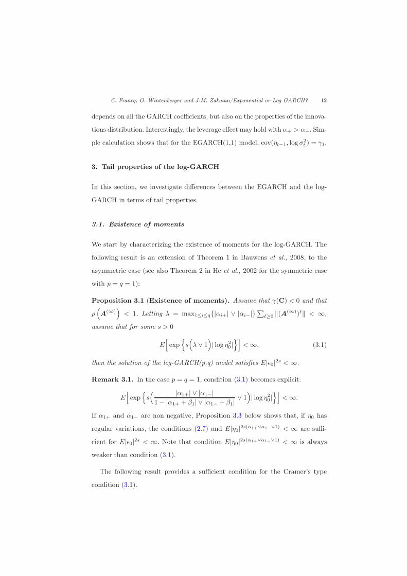
Proposition 3.1 (Existence of moments). Assume that γ(C) < 0 and that
ρ(A(∞)
)< 1. Letting λ = max1≤i≤q{|αi+| ∨ |αi−|}
∑ℓ≥0 ‖(A(∞))ℓ‖ < ∞,
assume that for some s > 0
E[exp
{s(λ ∨ 1
)| log η2
0 |}]
<∞, (3.1)
then the solution of the log-GARCH(p,q) model satisfies E|ǫ0|2s <∞.
Remark 3.1. In the case p = q = 1, condition (3.1) becomes explicit:
E[exp
{s( |α1+| ∨ |α1−|
1 − |α1+ + β1| ∨ |α1− + β1|∨ 1
)| log η2
0 |}]
<∞.
If α1+ and α1− are non negative, Proposition 3.3 below shows that, if η0 has
regular variations, the conditions (2.7) and E|η0|2s(α1+∨α1−∨1) < ∞ are suffi-
cient for E|ǫ0|2s < ∞. Note that condition E|η0|2s(α1+∨α1−∨1) < ∞ is always
weaker than condition (3.1).
The following result provides a sufficient condition for the Cramer’s type
condition (3.1).

C. Francq, O. Wintenberger and J-M. Zakoïan/Exponential or Log GARCH? 13
Proposition 3.2. If E(|η0|s) < ∞ for some s > 0 and η0 admits a den-
sity f around 0 such that f(y−1) = o(|y|δ) for δ < 1 when |y| → ∞ then
E exp(s1| log η20 |) <∞ for some s1 > 0.
For an explicit expression of the unconditional moments in the case of
symmetric log-GARCH(p, q) models, we refer the reader to Bauwens et al.
(2008).
3.2. Regular variation of the log-GARCH(1,1)
Under the assumptions of Proposition 2.3 we have an explicit expression of the
stationary solution. Thus it is possible to assert the regular variation proper-
ties of the log-GARCH model. Recall that L is a slowly varying function iff
L(xy)/L(x) → 1 as x → ∞ for any y > 0. A random variable X is said to be
regularly varying of index r > 0 if there exists a slowly varying function L and
p+ q = 1, p ∧ q ≥ 0 such that
P (X > x) ∼ px−rL(x) and P (X ≤ −x) ∼ qx−rL(x) x→ ∞.
The following proposition asserts the regular variation properties of the station-
ary solution of the log-GARCH(1,1) model.
Proposition 3.3 (Regular variation of the log-GARCH(1,1) model). Consider
the log-GARCH(1,1) model under (2.6) with α1+ ∧ α1− > 0. If (β1 + α1+) ∧(β1 + α1−) < 0, assume additionally that there exists c > 0 such that P (1/η >
t) ≤ cP (η > t) for all t ≥ 1.
• If η0 is regularly varying of index 2r > 0 then σ20 and ǫ0 are regularly
varying of index r/(α1+ ∨ α1−) and 2r/(α1+ ∨ α1− ∨ 1) respectively.
• If η0 has finite moments of order 2r > 0 then σ20 and ǫ0 have finite mo-
ments of order r/(α1+ ∨ α1−) and 2r/(α1+ ∨ α1− ∨ 1) respectively.

C. Francq, O. Wintenberger and J-M. Zakoïan/Exponential or Log GARCH? 14
The square root of the volatility σ0 can have heavier tails than the in-
novations when α1+ ∨ α1− > 1. Similarly, in the EGARCH(1,1) model the
observations can have a much heavier tail than the innovations. Moreover,
when the innovations are light tailed distributed (for instance exponentially
distributed), the EGARCH can exhibit regular variation properties. It is not
the case for the log-GARCH(1,1) model.
In this context of heavy tail, a natural way to deal with the dependence
structure is to study the multivariate regular variation of a trajectory. As the
innovations are independent, the dependence structure can only come from the
volatility process. However, it is also independent in the extremes. The following
is a straightforward application of Lemma 3.4 of Mikosch and Rezapour (2012).
Proposition 3.4 (Multivariate regular variation of the log-GARCH(1,1)
model). Assume the conditions of Proposition 3.3 satisfied. Then the sequence
(σ2t ) is regularly varying with index r/(α1+ ∨ α1−). The limit measure of the
vector Σ2d = (σ2
1 , . . . , σ2d)′ is given by the following limiting relation on the Borel
σ-field of (R ∪ {+∞})d/{0d}
P (x−1Σ2d ∈ ·)
P (σ2 > x)→ r
α1+ ∨ α1−
d∑
i=1
∫ ∞
1
y−r/(α1+∨α1−)−11{yei∈·}dy, x→ ∞.
where ei is the i-th unit vector in Rd and the convergence holds vaguely.
As for the innovations, the limiting measure above is concentrated on the
axes. Thus it is also the case for the log-GARCH(1,1) process and its extremes
values do not cluster. It is a drawback for modeling stock returns when clusters
of volatilities are stylized facts. This lack of clustering is also observed for the
EGARCH(1,1) model in Mikosch and Rezapour (2012), in contrast with the
GARCH(1,1) model, see Mikosch and Starica (2000).
We have seen that the extremal behavior of the log-GARCH model is similar
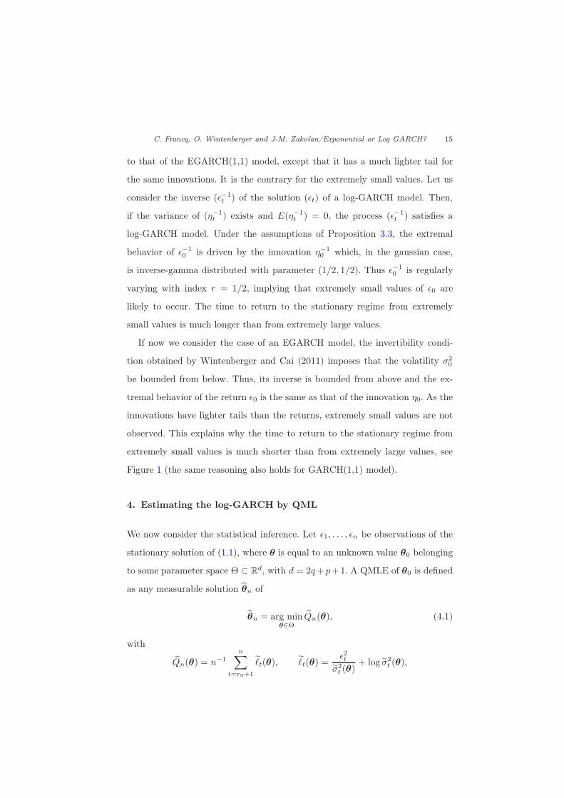
C. Francq, O. Wintenberger and J-M. Zakoïan/Exponential or Log GARCH? 15
to that of the EGARCH(1,1) model, except that it has a much lighter tail for
the same innovations. It is the contrary for the extremely small values. Let us
consider the inverse (ǫ−1t ) of the solution (ǫt) of a log-GARCH model. Then,
if the variance of (η−1t ) exists and E(η−1
t ) = 0, the process (ǫ−1t ) satisfies a
log-GARCH model. Under the assumptions of Proposition 3.3, the extremal
behavior of ǫ−10 is driven by the innovation η−1
0 which, in the gaussian case,
is inverse-gamma distributed with parameter (1/2, 1/2). Thus ǫ−10 is regularly
varying with index r = 1/2, implying that extremely small values of ǫ0 are
likely to occur. The time to return to the stationary regime from extremely
small values is much longer than from extremely large values.
If now we consider the case of an EGARCH model, the invertibility condi-
tion obtained by Wintenberger and Cai (2011) imposes that the volatility σ20
be bounded from below. Thus, its inverse is bounded from above and the ex-
tremal behavior of the return ǫ0 is the same as that of the innovation η0. As the
innovations have lighter tails than the returns, extremely small values are not
observed. This explains why the time to return to the stationary regime from
extremely small values is much shorter than from extremely large values, see
Figure 1 (the same reasoning also holds for GARCH(1,1) model).
4. Estimating the log-GARCH by QML
We now consider the statistical inference. Let ǫ1, . . . , ǫn be observations of the
stationary solution of (1.1), where θ is equal to an unknown value θ0 belonging
to some parameter space Θ ⊂ Rd, with d = 2q+p+1. A QMLE of θ0 is defined
as any measurable solution θ̂n of
θ̂n = arg minθ∈Θ
Q̃n(θ), (4.1)
with
Q̃n(θ) = n−1n∑
t=r0+1
ℓ̃t(θ), ℓ̃t(θ) =ǫ2t
σ̃2t (θ)
+ log σ̃2t (θ),
C. Francq, O. Wintenberger and J-M. Zakoïan/Exponential or Log GARCH? 16
where r0 is a fixed integer and log σ̃2t (θ) is recursively defined, for t = 1, 2, . . . , n,
by
log σ̃2t (θ) = ω +
q∑
i=1
(αi+1{ǫt−i>0} + αi−1{ǫt−i<0}
)log ǫ2t−i +
p∑
j=1
βj log σ̃2t−j(θ),
using positive initial values for ǫ20, . . . , ǫ21−q, σ̃
20(θ), . . . , , σ̃2
1−p(θ).
Remark 4.1 (On the choice of the initial values). The initial values can
be arbitrary positive numbers, for instance ǫ0 = · · · = ǫ1−q = σ̃0(θ) = · · · =
σ̃1−p(θ) =√
2 (for daily returns of stock market indices, in percentage, the
empirical variance is often close to 2). They can also depend on the parameter,
for instance ǫ0 = · · · = ǫ1−q = σ̃0(θ) = · · · = σ̃1−p(θ) = exp(ω/2). It is
also possible to take initial values depending on the observations, for instance
ǫ0 = · · · = ǫ1−q = σ̃0(θ) = · · · = σ̃1−p(θ) =√n−1
∑nt=1 ǫ
2t . It will be shown in
the sequel that the choice of r0 and of the initial values is unimportant for the
asymptotic behavior of the QMLE, provided r0 is fixed and there exists a real
random variable K independent of n such that
supθ∈Θ
∣∣log σ2t (θ) − log σ̃2
t (θ)∣∣ < K, a.s. for t = q − p+ 1, . . . , q, (4.2)
where σ2t (θ) is defined by (7.3) below. These conditions are supposed to hold in
the sequel.
Remark 4.2 (Our choice of the initial values). Even if the initial values do
not affect the asymptotic behavior of the QMLE, the finite sample value of θ̂n
is however quite sensitive to these values. Based on simulation experiments and
on illustrations on real data, for estimating log-GARCH(1,1) models we used
the empirical variance of the first 5 values (i.e. a week for daily data) as proxi
for the unknown value of σ21 . These initial values allow to compute σ̃2
t for t ≥ 2.
In order to attenuate the influence of the initial value without loosing too much
data, we chose r0 = 10.
Remark 4.3 (The empirical treatment of null returns). Under the as-
sumptions of Theorem 2.1, almost surely ǫ2t 6= 0. However, it may happen that

C. Francq, O. Wintenberger and J-M. Zakoïan/Exponential or Log GARCH? 17
some observations are equal to zero or are so close to zero that θ̂n cannot be
computed (the computation of the log ǫ2t ’s being required). To solve this poten-
tial problem, we imposed a lower bound for the |ǫt|’s. We took the lower bound
10−8, which is well inferior to a beep point, and we checked that nothing was
changed in the numerical illustrations presented here when this lower bound
was multiplied or divided by a factor of 100.
We now need to introduce some notation. For any θ ∈ Θ, let the polynomials
A+θ(z) =
∑qi=1 αi,+z
i, A−θ
(z) =∑q
i=1 αi,−zi and Bθ(z) = 1 − ∑p
j=1 βjzj. By
convention, A+θ(z) = 0 and A−
θ(z) = 0 if q = 0, and Bθ(z) = 1 if p = 0. We also
write C(θ0) instead of C to emphasize that the unknown parameter is θ0. The
following assumptions are used to show the strong consistency of the QMLE.
A1: θ0 ∈ Θ and Θ is compact.
A2: γ {C(θ0)} < 0 and ∀θ ∈ Θ, |Bθ(z)| = 0 ⇒ |z| > 1.
A3: The support of η0 contains at least two positive values and two negative
values, Eη20 = 1 and E| log η2
0 |s0 <∞ for some s0 > 0.
A4: If p > 0, A+θ0
(z) and A−θ0
(z) have no common root with Bθ0(z). More-
over A+θ0
(1) + A−θ0
(1) 6= 0 and |α0q+| + |α0q+| + |β0p| 6= 0.
A5: E∣∣log ǫ2t
∣∣ <∞.
Assumptions A1, A2 and A4 are similar to those required for the consistency
of the QMLE in standard GARCH models (see Berkes et al. 2003, Francq and
Zakoian, 2004). Assumption A3 precludes a mass at zero for the innovation,
and, for identifiability reasons, imposes non degeneracy of the positive and neg-
ative parts of η0. Note that, for other GARCH-type models, the absence of a
lower bound for the volatility can entail inconsistency of the QMLE (see Francq
and Zakoïan, 2010b). This is not the case for the log-GARCH under A5. Note
that this assumption can be replaced by the sufficient conditions given in Propo-
sition 2.2 (see also Examples 2.3 and 2.4).
Theorem 4.1 (Strong consistency of the QMLE). Let (θ̂n) be a sequence

C. Francq, O. Wintenberger and J-M. Zakoïan/Exponential or Log GARCH? 18
of QMLE satisfying (4.1), where the ǫt’s follow the asymmetric log-GARCH
model of parameter θ0. Under the assumptions (4.2) and A1-A5, almost surely
θ̂n → θ0 as n→ ∞.
Let us now study the asymptotic normality of the QMLE. We need the clas-
sical additional assumption:
A6: θ0 ∈◦
Θ and κ4 := E(η40) <∞.
Because the volatility σ2t is not bounded away from 0, we also need the following
non classical assumption.
A7: There exists s1 > 0 such that E exp(s1| log η20 |) <∞, and ρ(A(∞)) < 1.
The Cramer condition on | log η20 | in A7 is verified if ηt admits a density f
around 0 that does not explode too fast (see Proposition 3.2).
Let ∇Q = (∇1Q, . . . ,∇dQ)′ and HQ = (H1.Q′, . . . ,Hd.Q
′)′ be the vector
and matrix of the first-order and second-order partial derivatives of a function
Q : Θ → R.
Theorem 4.2 (Asymptotic normality of the QMLE). Under the assump-
tions of Theorem 4.1 and A6-A7, we have√n(θ̂n − θ0)
d→ N (0, (κ4 − 1)J−1)
as n→ ∞, where J = E[∇ log σ2t (θ0)∇ log σ2
t (θ0)′] is a positive definite matrix
andd→ denotes convergence in distribution.
It is worth noting that for the general EGARCH model, no similar results,
establishing the consistency and the asymptotic normality, exist. See however
Wintenberger and Cai (2011) for the EGARCH(1,1). The difficulty with the
EGARCH is to invert the volatility, that is to write σ2t (θ) as a well-defined
function of the past observables. In the log-GARCH model, invertibility reduces
to the standard assumption on Bθ given in A2.

C. Francq, O. Wintenberger and J-M. Zakoïan/Exponential or Log GARCH? 19
5. Asymmetric log-ACD model for duration data
The dynamics of duration between stock price changes has attracted much at-
tention in the econometrics literature. Engle and Russel (1997) proposed the
Autoregressive Conditional Duration (ACD) model, which assumes that the
duration between price changes has the dynamics of the square of a GARCH.
Bauwens and Giot (2000 and 2003) introduced logarithmic versions of the ACD,
that do not constrain the sign of the coefficients (see also Bauwens, Giot, Gram-
mig and Veredas (2004) and Allen, Chan, McAleer and Peiris (2008)). The asym-
metric ACD of Bauwens and Giot (2003) applies to pairs of observation (xi, yi),
where xi is the duration between two changes of the bid-ask quotes posted by a
market maker and yi is a variable indicating the direction of change of the mid
price defined as the average of the bid and ask prices (yi = 1 if the mid price
increased over duration xi, and yi = −1 otherwise). The asymmetric log-ACD
proposed by Bauwens and Giot (2003) can be written as
xi = ψizi,
logψi = ω +∑q
k=1
(αk+1{yi−k=1} + αk−1{yi−k=−1}
)log xi−k
+∑p
j=1 βj logψi−j ,
(5.1)
where (zi) is an iid sequence of positive variables with mean 1 (so that ψi can be
interpreted as the conditional mean of the duration xi). Note that ǫt :=√xtyt
follows the log-GARCH model (1.1), with ηt =√ztyt. Consequently, the results
of the present paper also apply to log-ACD models. In particular, the parameters
of (5.1) can be estimated by fitting model (1.1) on ǫt =√xtyt.
6. Numerical Applications
6.1. An application to exchange rates
We consider returns series of the daily exchange rates of the American Dollar
(USD), the Japanese Yen (JPY), the British Pound (BGP), the Swiss Franc

C. Francq, O. Wintenberger and J-M. Zakoïan/Exponential or Log GARCH? 20
Table 1
Log-GARCH(1,1) and EGARCH(1,1) models fitted by QMLE on daily returns of exchangerates. The estimated standard deviation are displayed into brackets.
Log-GARCH
ω̂ α̂+ α̂− β̂ Log-Lik.USD 0.024 (0.005) 0.027 (0.004) 0.016 (0.004) 0.971 (0.005) -0.104
JPY 0.051 (0.007) 0.037 (0.006) 0.042 (0.006) 0.952 (0.006) -0.354GBP 0.032 (0.006) 0.030 (0.005) 0.029 (0.005) 0.964 (0.006) 0.547
CHF 0.057 (0.012) 0.046 (0.008) 0.036 (0.007) 0.954 (0.008) 1.477CAD 0.021 (0.005) 0.025 (0.004) 0.017 (0.004) 0.969 (0.006) -0.170
EGARCH
ω̂ γ̂ δ̂ β̂ Log-Lik.USD -0.202 (0.030) -0.015 (0.014) 0.218 (0.031) 0.961 (0.010) -0.116JPY -0.152 (0.021) -0.061 (0.014) 0.171 (0.024) 0.970 (0.006) -0.334
GBP -0.447 (0.048) -0.029 (0.021) 0.420 (0.041) 0.913 (0.017) 0.503CHF -0.246 (0.046) -0.071 (0.022) 0.195 (0.035) 0.962 (0.009) 1.568
CAD -0.091 (0.017) -0.008 (0.010) 0.103 (0.019) 0.986 (0.005) -0.161
(CHF) and Canadian Dollar (CAD) with respect to the Euro. The observations
cover the period from January 5, 1999 to January 18, 2012, which corresponds
to 3344 observations. The data were obtained from the web site
http://www.ecb.int/stats/exchange/eurofxref/html/index.en.html.
Table 1 displays the estimated log-GARCH(1,1) and EGARCH(1,1) models
for each series. For all series, except the CHF, condition (2.7) ensuring the
existence of any log-moment is satisfied. Most of the estimated models present
asymmetries. However, the leverage effect is more visible in the EGARCH than
in the log-GARCH models. This is particularly apparent for the JPY model for
which γ̂ is clearly negative. For all models, the persistence parameter β is very
high. The last column shows that for the USD and the GBP, the log-GARCH has
a higher (quasi) log-likelihood than the EGARCH. The converse is true for the
three other assets. A study of the residuals, not reported here, is in accordance
with the better fit of one particular model for each series. This study confirms
that the models do not capture exactly the same empirical properties, and are
thus not perfectly substitutable.

C. Francq, O. Wintenberger and J-M. Zakoïan/Exponential or Log GARCH? 21
Table 2
Log-GARCH(1,1) models fitted on 5 simulations of a log-GARCH(1,1) model.
Iter ω̂ α̂+ α̂− β̂
1 0.025 (0.004) 0.028 (0.004) 0.018 (0.004) 0.968 (0.005)2 0.021 (0.003) 0.023 (0.003) 0.013 (0.003) 0.976 (0.004)3 0.026 (0.003) 0.028 (0.004) 0.017 (0.003) 0.969 (0.004)4 0.022 (0.003) 0.024 (0.004) 0.018 (0.003) 0.972 (0.004)5 0.024 (0.003) 0.028 (0.004) 0.014 (0.003) 0.974 (0.003)
Table 3
EGARCH(1,1) models fitted on 5 simulations of a log-GARCH(1,1) model.
Iter ω̂ γ̂ δ̂ β̂
1 -0.095 (0.016) -0.014 (0.009) 0.104 (0.017) 0.976 (0.006)2 -0.127 (0.018) 0.009 (0.010) 0.148 (0.021) 0.976 (0.007)3 -0.147 (0.018) 0.001 (0.010) 0.177 (0.022) 0.971 (0.007)4 -0.136 (0.019) -0.012 (0.010) 0.155 (0.022) 0.976 (0.007)5 -0.146 (0.019) -0.009 (0.010) 0.177 (0.023) 0.971 (0.007)
6.2. A Monte Carlo experiment
To evaluate the finite sample performance of the QML for the two models
we made the following numerical experiments. We first simulated the log-
GARCH(1,1) model, with n = 3344, ηt ∼ N (0, 1), and a parameter close to
those of Table 1, that is θ0 = (0.024, 0.027, 0.016, 0.971). Tables 2 and 3 display
the log-GARCH(1,1) and EGARCH(1,1) models fitted on these simulations. The
first table shows that the log-GARCH(1,1) is accurately estimated. In a second
time, we repeated the same experiments for simulations of an EGARCH(1,1)
model of parameter (ω0, γ0, δ0, β0) = (−0.204,−0.012, 0.227, 0.963). Tables 4
and 5 are the analogs of Tables 2 and 3 for the simulations of this EGARCH
model instead of the log-GARCH. Tables 5 indicates that the EGARCH are
satisfactorily estimated.

C. Francq, O. Wintenberger and J-M. Zakoïan/Exponential or Log GARCH? 22
Table 4
Log-GARCH(1,1) models fitted on 5 simulations of an EGARCH(1,1) model.
Iter ω̂ α̂+ α̂− β̂
1 0.039 (0.008) 0.071 (0.008) 0.052 (0.007) 0.874 (0.015)2 0.055 (0.006) 0.058 (0.007) 0.052 (0.006) 0.913 (0.010)3 0.052 (0.008) 0.070 (0.008) 0.060 (0.007) 0.873 (0.015)4 0.051 (0.008) 0.076 (0.008) 0.056 (0.007) 0.878 (0.014)5 0.056 (0.007) 0.061 (0.007) 0.060 (0.007) 0.896 (0.012)
Table 5
EGARCH(1,1) models fitted on 5 simulations of an EGARCH(1,1) model.
Iter ω̂ γ̂ δ̂ β̂
1 -0.220 (0.022) -0.024 (0.013) 0.235 (0.023) 0.950 (0.010)2 -0.196 (0.020) -0.029 (0.012) 0.219 (0.022) 0.961 (0.008)3 -0.222 (0.022) -0.005 (0.013) 0.241 (0.024) 0.947 (0.010)4 -0.227 (0.022) -0.025 (0.012) 0.248 (0.023) 0.950 (0.010)5 -0.209 (0.021) -0.003 (0.012) 0.234 (0.023) 0.955 (0.009)
7. Proofs
7.1. Proof of Theorem 2.1
Since the random variable ‖C0‖ is bounded, we have E log+ ‖C0‖ < ∞. The
moment condition on ηt entails that we also have E log+ ‖b0‖ < ∞. When
γ(C) < 0, Cauchy’s root test shows that, almost surely (a.s.), the series
zt = bt +
∞∑
n=0
CtCt−1 · · ·Ct−nbt−n−1 (7.1)
converges absolutely for all t and satisfies (2.2). A strictly stationary solution to
model (1.1) is then obtained as ǫt = exp{
12z2q+1,t
}ηt, where zi,t denotes the
i-th element of zt. This solution is non anticipative and ergodic, as a measurable
function of {ηu, u ≤ t}.We now prove that (7.1) is the unique nonanticipative solution of (2.2) when
γ(C) < 0. Let (z∗t ) be a strictly stationary process satisfying z∗
t = Ctz∗t−1 + bt.

C. Francq, O. Wintenberger and J-M. Zakoïan/Exponential or Log GARCH? 23
For all N ≥ 0,
z∗t = zt(N)+ Ct . . .Ct−Nz∗
t−N−1, zt(N) = bt +N∑
n=0
CtCt−1 · · ·Ct−nbt−n−1.
We then have
‖zt − z∗t ‖ ≤
∥∥∥∥∥
∞∑
n=N+1
CtCt−1 · · ·Ct−nbt−n−1
∥∥∥∥∥ + ‖Ct . . .Ct−N‖‖z∗t−N−1‖.
The first term in the right-hand side tends to 0 a.s. when N → ∞. The second
term tends to 0 in probability because γ(C) < 0 entails that ‖Ct . . .Ct−N‖ → 0
a.s. and the distribution of ‖z∗t−N−1‖ is independent of N by stationarity. We
have shown that zt − z∗t → 0 in probability when N → ∞. This quantity being
independent of N we have zt = z∗t a.s. for any t. ✷
7.2. Proof of Proposition 2.1
Let X be a random variable such that X > 0 a.s. and EXr < ∞ for
some r > 0. If E logX < 0, then there exists s > 0 such that EXs < 1
(see e.g. Lemma 2.3 in Berkes, Horváth and Kokoszka, 2003). Noting that
E ‖Ct · · ·C1‖ ≤ (E ‖C1‖)t < ∞ for all t, the previous result shows that when
γ(C) < 0 we have E‖Ck0· · ·C1‖s < 1 for some s > 0 and some k0 ≥ 1. One
can always assume that s < 1. In view of (7.1), the cr-inequality and stan-
dard arguments (see e.g. Corollary 2.3 in Francq and Zakoïan, 2010a) entail
that E‖zt‖s < ∞, provided E‖bt‖s < ∞, which holds true when s ≤ s0. The
conclusion follows. ✷
7.3. Proof of Proposition 2.2
By (2.4), componentwise we have
Abs(σt,r) ≤ Abs(ut) +
∞∑
ℓ=0
At,ℓAbs(ut−ℓ−1), At,ℓ :=
ℓ∏
j=0
Abs(At−j), (7.2)

C. Francq, O. Wintenberger and J-M. Zakoïan/Exponential or Log GARCH? 24
where each element of the series is defined a priori in [0,∞]. In view of the form
(2.3) of the matrices At, each element of
At,ℓAbs(ut−ℓ−1) = |ut−ℓ−1|ℓ∏
j=0
Abs(At−j)e1
is a sum of products of the form |ut−ℓ−1|∏k
j=0 |µℓj(ηt−ij
)| with 0 ≤ k ≤ ℓ and
0 ≤ i0 < · · · < ik ≤ ℓ + 1. To give more detail, consider for instance the case
r = 3. We then have
At,1Abs(ut−2) =
|µ1(ηt−1)||µ1(ηt−2)||ut−2| + |µ2(ηt−2)||ut−2||µ1(ηt−2)||ut−2|
|ut−2|
.
Noting that |ut−ℓ−1| is a function of ηt−ℓ−2 and its past values, we
obtain EAt,1Abs(ut−2) = EAbs(At)EAbs(At−1)EAbs(ut−2). More gen-
erally, it can be shown by induction on ℓ that the i-th element
of the vector At−1,ℓ−1Abs(ut−ℓ−1) is independent of the i-th element
of the first row of Abs(At). It follows that EAt,ℓAbs(ut−ℓ−1) =
EAbs(At)EAt−1,ℓ−1Abs(ut−ℓ−1). The property extends to r 6= 3. Therefore,
although the matrices involved in the product At,ℓAbs(ut−ℓ−1) are not inde-
pendent (in the case r > 1), we have
EAt,ℓAbs(ut−ℓ−1) =
ℓ∏
j=0
EAbs(At−j)EAbs(ut−ℓ−1)
=(A(1)
)ℓ+1
EAbs(u1).
In view of (7.2), the condition ρ(A(1)) < 1 then entails that EAbs(σt,r) is finite.
The case r = 1 is treated by noting that At,ℓAbs(ut−ℓ−1) is a product of
independent random variables.
To deal with the cases r 6= 1 and m 6= 1, we work with (2.2) instead of (2.4).
This Markovian representation has an higher dimension but involves indepen-
dent coefficients Ct. Define Ct,ℓ by replacing At−j by Ct−j in At,ℓ. We then

C. Francq, O. Wintenberger and J-M. Zakoïan/Exponential or Log GARCH? 25
have
EC⊗mt,ℓ Abs(bt−ℓ−1)
⊗m =(C(m)
)ℓ+1
EAbs(b1)⊗m.
For all m ≥ 1, let ‖M‖m = (E‖M‖m)1/m where ‖M‖ is the sum of the
absolute values of the elements of the matrix M . Using the elementary rela-
tions ‖M‖‖N‖ = ‖M ⊗ N‖ and E‖Abs(M)‖ = ‖EAbs(M )‖ for any ma-
trices M and N , the condition ρ(C(m)) < 1 entails E ‖Ct,ℓAbs(bt−ℓ−1)‖m=
‖EC⊗mt,ℓ Abs(bt−ℓ−1)
⊗m‖ → 0 at the exponential rate as ℓ→ ∞, and thus
‖Abs(zt)‖m ≤ ‖Abs(bt)‖m +
∞∑
ℓ=0
‖Ct,ℓAbs(bt−ℓ−1)‖m <∞,
which allows to conclude. ✷
7.4. Proof of Proposition 2.3
By the concavity of the logarithm function, the condition |α+ + β||α− + β| < 1
is satisfied. By Example 2.1 and the symmetry of the distribution of η0, the
existence of a strictly stationary solution process (ǫt) is thus guaranteed. By
2.3, this solution satisfies E| log ǫ2t | <∞. Let
at = (α+1{ηt>0} + α−1{ηt<0})ηt, bt = (α+1{ηt>0} + α−1{ηt<0})ηt log η2t .
We have
Eat = (α+ − α−)E(η01{η0>0}), Ebt = (α+ − α−)E(η0 log η201{η0>0}),
using the symmetry assumption for the second equality. Thus
cov(ηt−1, log(σ2t )) = E[at−1 log(σ2
t−1) + bt−1],
and the conclusion follows. ✷

C. Francq, O. Wintenberger and J-M. Zakoïan/Exponential or Log GARCH? 26
7.5. Proof of Proposition 3.1
By definition, | log(σ2t )| ≤ ‖σt,r‖ = ‖Abs(σt,r)‖. Then, we have
E|σ2t |s ≤ E {exp(s‖Abs(σt,r)‖)} =
∞∑
k=0
sk‖Abs(σt,r)‖kk
k!
≤∞∑
k=0
sk‖Abs(u0)‖kk
{∑∞ℓ=0 ‖(A(∞))ℓ‖
}k
k!
= E exp
{s‖Abs(u0)‖
∞∑
ℓ=0
‖(A(∞))ℓ‖},
where the last inequality comes from (2.5). By definition u0 = (u0, 0′r−1)
′ with
u0 = ω +
q∑
i=1
(αi+1η−i>0 + αi−1η−i<0) log η2−i.
Thus ‖Abs(u0)‖ ≤ |u0| ≤ |ω| + max1≤i≤q |αi+| ∨ |αi−|∑q
j=1 | log η2−j | and it
follows that
E|σ2t |s ≤ exp
{s|ω|
∞∑
ℓ=0
‖(A(∞))ℓ‖}
{E exp
(sλ| log η2
0 |)}q
<∞
under (3.1). ✷
7.6. Proof of Proposition 3.2
Without loss of generality assume that f exists on [−1, 1]. Then there exists
M > 0 such that f(1/y) ≤M |y|δ for all y ≥ 1 and we obtain
E exp(s1| log η20 |) ≤
∫
|x|<1
exp(2s1 log(1/x))f(x)dx +
∫exp(s1 log(x2))dPη(x)
≤ 2M
∫ ∞
1
y2(s1−1)+δdy + E(|η0|2s1 ).
The upper bound is finite for sufficiently small s1 and the result is proved. ✷

C. Francq, O. Wintenberger and J-M. Zakoïan/Exponential or Log GARCH? 27
7.7. Proof of Proposition 3.3
To prove the first assertion, note that if η0 is regularly varying of index 2r then η20
is regularly varying of index r. Thus u1 = ω+(α1+1{η0>0}+α1−1{η0<0}) log(η20)
is such that
P (eu0 > x) = P (η0 > 0)P(η20
α1+> xe−ω | η0 > 0
)
+P (η0 < 0)P(η20
α1−> xe−ω | η0 < 0
).
Then eu0 is also regularly varying with index r/(α1+)∧r/(α1−). An application
Lemma 3.3 in Mikosch and Rezapour (2012) yields the first assertion. The second
assertion follows easily by independence of η0 and σ0 with respective regularly
variation indexes r and r/(α1+ ∨ α1−). ✷
7.8. Proof of Theorem 4.1
We will use the following standard result (see e.g. Exercise 2.11 in Francq and
Zakoian, 2010a).
Lemma 7.1. Let (Xn) be a sequence of random variables. If supnE|Xn| <∞,
then almost surely n−1Xn → 0 as n → ∞. The almost sure convergence may
fail when supn E|Xn| = ∞. If the sequence (Xn) is bounded in probability, then
n−1Xn → 0 in probability.
Turning to the proof of Theorem 4.1, first note that A2, A3 and Proposi-
tion 2.1 ensure the a.s. absolute convergence of the series
log σ2t (θ) := B−1
θ(B)
{ω +
q∑
i=1
(αi+1{ǫt−i>0} + αi−1{ǫt−i<0}
)log ǫ2t−i
}. (7.3)
Let
Qn(θ) = n−1n∑
t=r0+1
ℓt(θ), ℓt(θ) =ǫ2t
σ2t (θ)
+ log σ2t (θ).
Using standard arguments, as in the proof of Theorem 2.1 in Francq and Za-
koian (2004) (hereafter FZ), the consistency is obtained by showing the following

C. Francq, O. Wintenberger and J-M. Zakoïan/Exponential or Log GARCH? 28
intermediate results
i) limn→∞
supθ∈Θ
|Qn(θ) − Q̃n(θ)| = 0 a.s.;
ii) if σ21(θ) = σ2
1(θ0) a.s. then θ = θ0;
iii) if θ 6= θ0 , Eℓt(θ) > Eℓt(θ0);
iv) any θ 6= θ0 has a neighborhood V (θ) such that
lim infn→∞
infθ∗∈V (θ)
Q̃n(θ∗) > Eℓt(θ0) a.s.
Because of the multiplicative form of the volatility, the step i) is more delicate
than in the standard GARCH case. In the case p = q = 1, we have
log σ2t (θ) − log σ̃2
t (θ) = βt−1{log σ2
1(θ) − log σ̃21(θ)
}, ∀t ≥ 1.
In the general case, as in FZ, using (4.2) one can show that for almost all
trajectories,
supθ∈Θ
∣∣log σ2t (θ) − log σ̃2
t (θ)∣∣ ≤ Kρt, (7.4)
where ρ ∈ (0, 1) and K > 0. When the initial values are chosen as suggested
by Remark 4.2, K is the realization of a random variable which is measurable
with respect to σ ({ηu, u ≤ 5}). First complete the proof of i) in the case p =
q = 1 and α+ = α−, for which the notation is more explicit. In view of the
multiplicative form of the volatility
σ2t (θ) = eβt−1 log σ2
1(θ)t−2∏
i=0
eβi{ω+α log ǫ2t−1−i}, (7.5)
we have
1
tlog
∣∣∣∣1
σ2t (θ)
− 1
σ̃2t (θ)
∣∣∣∣ =−1
t
t−2∑
i=0
βi{ω + α log ǫ2t−1−i
}
+1
tlog
∣∣∣e−βt−1 log σ21(θ) − e−βt−1 log σ̃2
1(θ)∣∣∣ .
Applying Lemma 7.1, the first term of the right-hand side of the equality tends
almost surely to zero because it is bounded by a variable of the form |Xt|/t,

C. Francq, O. Wintenberger and J-M. Zakoïan/Exponential or Log GARCH? 29
with E|Xt| <∞, under A5. The second term is equal to
1
tlog
∣∣∣{log σ2
1(θ) − log σ̃21(θ)
}βt−1e−βt−1x∗
∣∣∣ ,
where x∗ is between log σ21(θ) and log σ̃2
1(θ). This second term thus tends to
log |β| < 0 when t→ ∞. It follows that
supθ∈Θ
∣∣∣∣1
σ2t (θ)
− 1
σ̃2t (θ)
∣∣∣∣ ≤ Kρt, (7.6)
where K and ρ are as in (7.4). Now consider the general case. Iterating (1.1),
using the compactness of Θ and the second part of A2, we have
log σ2t (θ) =
t−1∑
i=1
ci(θ) + ci+(θ)1{ǫt−i>0} log ǫ2t−i + ci−(θ)1{ǫt−i<0} log ǫ2t−i
+
p∑
j=1
ct,j(θ) log σ2q+1−j(θ)
with
supθ∈Θ
max{|ci(θ)|, |ci+(θ)|, |ci−(θ)|, |ci,1(θ)|, . . . , |ci,p(θ)|} ≤ Kρi, ρ ∈ (0, 1).
(7.7)
We then obtain a multiplicative form for σ2t (θ) which generalizes (7.5), and
deduce that1
tlog
∣∣∣∣1
σ2t (θ)
− 1
σ̃2t (θ)
∣∣∣∣ = a1 + a2,
where
a1 =−1
t
t−1∑
i=1
ci(θ)+ ci+(θ)1{ǫt−i>0} log ǫ2t−i + ci−(θ)1{ǫt−i<0} log ǫ2t−i → 0 a.s.
in view of (7.7) and Lemma 7.1, and for x∗j ’s between log σ2q+1−j(θ) and
log σ̃2q+1−j(θ),
a2 =1
tlog
∣∣∣∣∣exp
{−
p∑
j=1
ct,j(θ) log σ2q+1−j(θ)
}− exp
{−
p∑
j=1
ct,j(θ) log σ̃2q+1−j(θ)
}∣∣∣∣∣
=1
tlog
∣∣∣∣∣−p∑
j=1
ct,j(θ){log σ
2q+1−j(θ)− log σ
2q+1−j(θ)
}exp
{−
p∑
k=1
ct,k(θ) log x∗
k
}∣∣∣∣∣
=1
tlog
∣∣∣∣∣−p∑
j=1
ct,j(θ)
∣∣∣∣∣ + o(1) a.s.

C. Francq, O. Wintenberger and J-M. Zakoïan/Exponential or Log GARCH? 30
using (4.2) and (7.7). Using again (4.2), it follows that lim supn→∞ a2 ≤ log ρ <
0. We conclude that (7.6) holds true in the general case. The proof of i) then
follows from (7.4)-(7.6), as in FZ.
To show ii), note that we have
Bθ(B) log σ2t (θ) = ω + A+
θ(B)1{ǫt>0} log ǫ2t + A−
θ(B)1{ǫt<0} log ǫ2t . (7.8)
If log σ21(θ) = log σ2
1(θ0) a.s., by stationarity we have log σ2t (θ) = log σ2
t (θ0) for
all t, and thus we have almost surely
{A+
θ(B)
Bθ(B)−
A+θ0
(B)
Bθ0(B)
}1{ǫt>0} log ǫ2t +
{A−
θ(B)
Bθ(B)−
A−θ0
(B)
Bθ0(B)
}1{ǫt<0} log ǫ2t
=ω0
Bθ0(1)
− ω
Bθ(1).
Denote by Rt any random variable which is measurable with respect to
σ ({ηu, u ≤ t}). If
A+θ
(B)
Bθ(B)6=
A+θ0
(B)
Bθ0(B)
orA−
θ(B)
Bθ(B)6=
A−θ0
(B)
Bθ0(B)
, (7.9)
there exists a non null (c+, c−)′ ∈ R2, such that
c+1{ηt>0} log ǫ2t + c−1{ηt<0} log ǫ2t +Rt−1 = 0 a.s.
This is equivalent to the two equations
(c+ log η2
t + c+ log σ2t +Rt−1
)1{ηt>0} = 0
and(c− log η2
t + c− log σ2t +Rt−1
)1{ηt<0} = 0.
Note that if an equation of the form a logx21{x>0} + b1{x>0} = 0 admits two
positive solutions then a = 0. This result, A3, and the independence between
ηt and (σ2t , Rt−1) imply that c+ = 0. Similarly we obtain c− = 0, which leads
to a contradiction. We conclude that (7.9) cannot hold true, and the conclusion
follows from A4.

C. Francq, O. Wintenberger and J-M. Zakoïan/Exponential or Log GARCH? 31
Since σ2t (θ) is not bounded away from zero, the beginning of the proof of iii)
slightly differs from that given by FZ in the standard GARCH case. In view of
(7.8), the second part of A2 and A5 entail that E| log σ2t (θ)| <∞ for all θ ∈ Θ.
It follows that Eℓ−t (θ) <∞ and E|ℓt(θ0)| <∞.
The rest of the proof of iii), as well as that of iv), are identical to those given
in FZ. ✷
7.9. Proof of Theorem 4.2
A Taylor expansion gives
∇iQn(θ̂n) −∇iQn(θ0) = Hi.Qn(θ̃n,i)(θ̂n − θ0) for all 1 ≤ i ≤ d,
where the θ̃n,i’s are such that ‖θ̃n,i−θ0‖ ≤ ‖θ̂n−θ0‖. As in Section 5 of Bardet
and Wintenberger (2009), the asymptotic normality is obtained by showing:
1. n1/2∇Qn(θ0) → N (0, (κ4 − 1)J),
2. ‖HQn(θ̃n) − J‖ converges a.s. to 0 for any sequence (θ̃n) converging a.s.
to θ0 and J is invertible,
3. n1/2‖∇Q̃n(θ̂n) −∇Qn(θ̂n)‖ converges a.s. to 0.
In order to prove the points 1-3 we will use the following Lemma
Lemma 7.2. Under the assumptions of Theorem 4.1 and A7, for any m > 0
there exists a neighborhood V of θ0 such that E[supV(σ2t /σ
2t (θ))m] < ∞ and
E[supV | log σ2t (θ)|m] <∞.
Proof. We have
log σ2t (θ0) − log σ2
t (θ) = ω0 − ω +
p∑
j=1
βj{log σ2t−j(θ0) − log σ2
t−j(θ)}
+Vθ0−θσt−1,r + A+θ0−θ
(B)1ηt>0 log η2t + A−
θ0−θ(B)1ηt<0 log η2
t
with σt,r = (log σ2t (θ0), . . . , log σ2
t−r+1(θ0))′,
Vθ = (α1+1{ηt−1>0}+α1−1{ηt−1<0}+β1, . . . , αr+1{ηt−r>0}+αr−1{ηt−r<0}+βr).

C. Francq, O. Wintenberger and J-M. Zakoïan/Exponential or Log GARCH? 32
Under A2, we then have
log σ2t (θ0) − log σ2
t (θ) = B−1θ
(B) {ω0 − ω + Vθ0−θσt−1,r
+(A+θ0−θ
(B)1ηt>0 log η2t + A−
θ0−θ(B)1ηt<0 log η2
t
}.
Under A7 the assumptions of Proposition 3.1 hold. From the proof of that
proposition, we thus have that E exp(δ‖Abs(σt,r)‖) is finite for some δ > 0.
Now, note that Vθ, A+θ(1) and A+
θ(1) are continuous functions
of θ. Choosing a sufficiently small neighborhood V of θ0, one can
make supV ‖Vθ0−θ‖, supV |A+θ0−θ
(1)| and supV |A+θ0−θ
(1)| arbitrarily small.
Thus E[exp(m supV ‖Vθ0−θσt,r‖)] and E[exp(m supV ‖(A+θ0−θ
(B)1ηt−1>0 +
A−θ0−θ
(B)1ηt−1<0) log(η2t−1)‖)] are finite for an appropriate choice of V depend-
ing on m. We conclude that E[exp
(m supV
∣∣log{σ2
t (θ0)/σ2t (θ)
}∣∣)] < ∞ and
the first assertion of the lemma is proved.
Consider now the second assertion. We have
supV
| log σ2t (θ)| ≤ | log σ2
t | + supV
| log(σ2t (θ0)/σ
2t (θ))|.
We have already shown that the second term admits a finite moment of order
m. So does the first term, under A7, by Remark 2.2. �
Now let us prove that the point 1. follows from the fact that ∇Qn(θ0) is a
martingale in L2. Indeed
∇Qn(θ0) = n−1n∑
t=r0+1
(1 − η2t )∇ log σ2
t (θ0).
As ηt is independent of log σ2t (θ0) and Eη2
t = 1 the Central Limit
Theorem for martingale differences applies whenever Q = (κ4 −1)E(∇ log σ2
t (θ0)∇ log σ2t (θ0)
′) exists. For any θ ∈◦
Θ, the random vector

C. Francq, O. Wintenberger and J-M. Zakoïan/Exponential or Log GARCH? 33
∇ log σ2t (θ) is the stationary solution of the equation
∇ log σ2t (θ) =
p∑
j=1
βj∇ log σ2t−j(θ) +
1
ǫ+t−1,q
ǫ−t−1,q
σ2t−1,p(θ)
, (7.10)
where σ2t,p(θ) = (log σ2
t (θ), . . . , log σ2t−p+1(θ))′.
Assumption A2 entails that ∇ log σ2t (θ) is a linear combination of ǫ+
t−i,q,
ǫ−t−i,q and log σ2t−i(θ) for i ≥ 1. Lemma 7.2 ensures that, for any m > 0,
there exists a neighborhood V of θ0 such that E[supV | log σ2t−i(θ)|m] < ∞.
By Remark 2.2, ǫ+t−i,q and ǫ−t−i,q admit moments of any order. Thus, for any
m > 0 there exists V such that E[supV ‖∇ logσ2t (θ)‖m] < ∞. In particular,
∇ log σ2t (θ0) admits moments of any order. Thus point 1. is proved.
Turning to point 2., we have
HQn(θ) = n−1n∑
t=r0+1
Hℓt(θ),
where
Hℓt(θ) =
(1 − η2
t σ2t (θ0)
σ2t (θ)
)H logσ2
t (θ) +η2
t σ2t (θ0)
σ2t (θ)
∇ log σ2t (θ)∇ log σ2
t (θ)′.
(7.11)
By Lemma 7.2, the term σ2t (θ0)/σ
2t (θ) admits moments of order as large as we
need uniformly on a well chosen neighborhood V of θ0. Let us prove that it is
also the case for H logσ2t (θ). Computation gives
H logσ2t (θ) =
p∑
j=1
βjH log σ2t−j(θ) +
0(2q+1)×d
∇′σ2t−1,p(θ)
+
0(2q+1)×d
∇′σ2t−1,p(θ)
′
.
From this relation and A2 we obtain
H log σ2t (θ) =
0(2q+1)×d
Bθ(B)−1∇′σ2t−1,p(θ)
+
0(2q+1)×d
Bθ(B)−1∇′σ2t−1,p(θ)
′
.
Thus H logσ2t (θ) belongs to C(V) and is integrable because we can always choose
V such that supV ‖∇′σ2t−1,p(θ)‖ ∈ Lm (see the proof of point 1. above).
C. Francq, O. Wintenberger and J-M. Zakoïan/Exponential or Log GARCH? 34
An application of the Cauchy-Schwarz inequality in the RHS term of (7.11)
yields the integrability of supV Hℓt(θ). The first assertion of point 2. is proved
by an application of the ergodic theorem on (Hℓt(θ)) in the Banach space C(V)
equipped with the supremum norm:
supV
‖HQn(θ) − E[Hℓ0(θ)]‖ → 0 a.s.
An application of Theorem 4.1 ensures that θ̂n belongs a.s. to V for sufficiently
large n. Thus
‖HQn(θ̂n)−E[Hℓ0(θ0)]‖ ≤ supV
‖HQn(θ)−E[Hℓ0(θ)]‖+‖E[Hℓ0(θ̂n)]−E[Hℓ0(θ0)]‖
converges a.s. to 0 by continuity of θ → E[Hℓ0(θ)] at θ0 as a consequence of a
dominating argument on V . The first assertion of point 2. is proved.
The matrix J is non invertible iff there exists a non null deterministic vector
λ = (λ0, λ1, . . . , λp+2q)′ such that λ′ ∇ log σ2
t (θ0) = 0 a.s. If the latter equality
holds, (7.10) entails (1, ǫ+t,q, ǫ
−t,q,σ
2t,p(θ0))λ = 0 a.s. By A3 and arguments
used for proving the point (ii) in the proof of Theorem 4.1, we deduce λp+1 =
λp+q+1 = 0. For the same reason if λ1 = · · · = λi = 0 then λp+2 = · · · =
λp+1+i = 0 and λp+q+2 = · · · = λp+q+1+i = 0 for 1 ≤ i ≤ p ∧ q. Thus as
λ 6= 0 there exists λk 6= 0 for 1 ≤ k ≤ q such that λj = 0 for j < k. Then,
log(σ2t−k) is a linear combination of (log(σ2
t−j))k<j≤q , (1{ǫt−j>0} log(ǫ2t−j))k<j≤p
and (1{ǫt−j<0} log(ǫ2t−j))k<j≤p. We thus find a log-GARCH(p′, q′) representation
with p′ < p and q′ < q, in contradiction with A4. Thus J is invertible.
From (7.10) and an equivalent representation for ∇ log σ̃2t (θ), we have
∇ log σ2t (θ) −∇ log σ̃2
t (θ) =
p∑
j=1
βj(∇ log σ2t−j(θ) −∇ log σ̃2
t−j(θ))
+
02q+1
σ2t−1,p(θ) − σ̃
2t−1,p(θ)

C. Francq, O. Wintenberger and J-M. Zakoïan/Exponential or Log GARCH? 35
where σ̃2t,p is defined as σ2
t,p. Thus, there exist continuous functions di and dt,i
defined on Θ such that
∇ log σ2t (θ) −∇ log σ̃2
t (θ) =
t−1∑
i=1
di(θ)(log σ2t−i(θ) − log σ̃2
t−i(θ))
+
p∑
j=1
dt,j(θ)∇ log σ2p+1−j(θ).
The sequences of functions (di), (di,j), 1 ≤ j ≤ p, satisfy the same uniform
rate of convergence as the functions ci, ci+, c1− and ci,j in (7.7). An appli-
cation of (7.4) yields to the existence of K > 0 and ρ ∈ (0, 1) such that
supΘ ‖∇ logσ2t (θ) − ∇ log σ̃2
t (θ)‖ ≤ Kρt, for almost all trajectories. Point 3.
follows easily and the asymptotic normality is proved. ✷
8. Conclusion
In this paper, we investigated the probabilistic properties of the log-
GARCH(p, q) model. We found sufficient conditions for the existence of moments
and log-moments of the strictly stationary solutions. We analyzed the depen-
dence structure through the leverage effect and the regular variation properties,
and we compared this structure with that of the EGARCH model.
As far as the estimation is concerned, it should be emphasized that the
log-GARCH model appears to be much more tractable than the EGARCH.
Indeed, we established the strong consistency and the asymptotic normality
of the QMLE under mild assumptions. For EGARCH models, such properties
have only been established for the first-order model and with strong invertibil-
ity constraints (see Wintenberger and Cai, 2011). By comparison with standard
GARCH, the log-GARCH model is not more difficult to handle: on the one
hand, the fact that the volatility is not bounded below requires an additional
log-moment assumption, but on the other hand the parameters are nor positively
constrained.

C. Francq, O. Wintenberger and J-M. Zakoïan/Exponential or Log GARCH? 36
A natural extension of this work, aiming at pursuing the comparison between
the two classes of models, would rely on statistical tests. By embedding the
log-GARCH model in a more general framework including the log-GARCH, it
should be possible to consider a LM test of the log-GARCH null assumption.
Another problem of interest would be to check validity of the estimated models.
We leave these issues for further investigation, viewing the results of this paper
as a first step in these directions.
References
Allen, D. , Chan, F., McAleer, M., and Peiris, S. (2008) Finite sample
properties of the QMLE for the log-ACD model: Application to Australian
stocks. Journal of Econometrics 147, 163–183.
Bardet, J.-M. and Wintenberger, O. (2009) Asymptotic normality of the
Quasi Maximum Likelihood Estimator for multidimensional causal pro-
cesses. Ann. Statist. 37, 2730–2759.
Bauwens, L. and Giot, P. (2000) The logarithmic ACD model: An appli-
cation to the bidask quote process of three NYSE stocks. Annales
D’Economie et de Statistique 60, 117–145.
Bauwens, L. and Giot, P. (2003) Asymmetric ACD models: introducing
price information in ACD models. Empirical Economics 28, 709–731.
Bauwens, L., Galli, F. and Giot, P. (2008) The moments of log-ACD mod-
els. QASS 2, 1–28.
Bauwens, L., Giot, P., Grammig, J. and Veredas, D. (2004) A compar-
ison of financial duration models via density forecast. International Jour-
nal of Forecasting 20, 589–604.
Berkes, I., Horváth, L. and Kokoszka, P. (2003) GARCH processes:
structure and estimation. Bernoulli 9, 201–227.
Bollerslev, T. (1986) Generalized autoregressive conditional heteroskedastic-

C. Francq, O. Wintenberger and J-M. Zakoïan/Exponential or Log GARCH? 37
ity. Journal of Econometrics 31, 307–327.
Bougerol, P. and Picard, N. (1992a) Strict stationarity of generalized au-
toregressive processes. Annals of Probability 20, 1714–1729.
Bougerol, P. and Picard, N. (1992b) Stationarity of GARCH processes and
of some nonnegative time series. Journal of Econometrics 52, 115–127.
Drost, F.C. and Nijman, T.E. (1993) Temporal Aggregation of GARCH
Processes. Econometrica 61, 909–927.
Engle, R.F. (1982) Autoregressive Conditional Heteroskedasticity with Esti-
mates of the Variance of U.K. Inflation. Econometrica 50, 987–1008.
Engle, R.F. and Russell, J.R. (1998) Autoregressive Conditional Duration:
A New Model for Irregularly Spaced Transaction Data. Econometrica 66,
1127–1162.
Francq, C. and Zakoïan, J-M. (2004) Maximum Likelihood Estimation of
Pure GARCH and ARMA-GARCH. Bernoulli 10, 605–637.
Francq, C. and Zakoïan, J-M. (2010a) GARCH Models : structure, statis-
tical inference and financial applications. John Wiley.
Francq, C. and Zakoïan, J-M. (2010b) Inconsistency of the MLE and infer-
ence based on weighted LS for LARCH models. Journal of Econometrics
159, 151–165.
Geweke, J. (1986) Modeling the Persistence of Conditional Variances: A Com-
ment. Econometric Review 5, 57–61.
He, C., Teräsvirta, T. and Malmsten, H. (2002) Moment structure of a
family of first-order exponential GARCH models. Econometric Theory 18,
868–885.
Mikosch, T. and Rezapour, M. (2012) Stochastic volatility models with
possible extremal clustering. Bernoulli To appear.
Mikosch, T. and Starica, C. (2000) Limit theory for the sample autocor-
relations and extremes of a GARCH (1,1) process. Ann. Statist. 28,
1427?1451.

C. Francq, O. Wintenberger and J-M. Zakoïan/Exponential or Log GARCH? 38
Milhøj, A. (1987) A Multiplicative Parameterization of ARCH Models. Work-
ing paper, Department of Statistics, University of Copenhagen.
Nelson D.B. (1991) Conditional Heteroskedasticity in Asset Returns : a New
Approach. Econometrica 59, 347–370.
Pantula, S.G. (1986) Modeling the Persistence of Conditional Variances: A
Comment. Econometric Review 5, 71–74.
Sucarrat, G. and Escribano, A. (2010) The Power Log-GARCH Model.
Working document, Economic Series 10-13, University Carlos III, Madrid.
Sucarrat, G. and Escribano, A. (2012) Automated Model Selection in Fi-
nance: General-to-Specific Modelling of the Mean and Volatility Specifi-
cations. Oxford Bulletin Of Economics And Statistics 74, 716–735.
Wintenberger, O. and Cai, S. (2011) Parametric inference and forecasting
in continuously invertible volatility models. Preprint arXiv:1106.4983v3.