Game Theory | Lecture 3morri/comp9514/lecture3.pdf · Game Theory | Lecture 3 9 Slide 17 ' & $ %...

COMP9514, 1998 Game Theory | Lecture 3 1

Slide 1

'

&

$

%

Maurice Pagnucco

Knowledge Systems Group

Department of Arti�cial Intelligence

School of Computer Science and Engineering

The University of New South Wales

NSW 2052, AUSTRALIA

[email protected]

Slide 2

'

&

$

%

Game Trees

Matrix games assume players choose strategy simultaneously without

knowledge of what other player is choosing

In real situations decisions made sequentially and information about

previous choices becomes available to players as situation develops

We shall introduce another way of modelling situations


Slide 3

'

&

$

%

Structure of Game Trees

A game tree is structured as follows:

Each node labelled by player making choice

Each branch labelled with particular choice (of action) made by

player

Each leaf node labelled with payo� to players (convention: payo� to

one of the players)

Chance events (e.g., roll of die, dealing of cards, . . . ) must also be

represented

In this case, node labelled Chance and branches labelled with

probability that Chance will come up with that choice

Slide 4

'

&

$

%

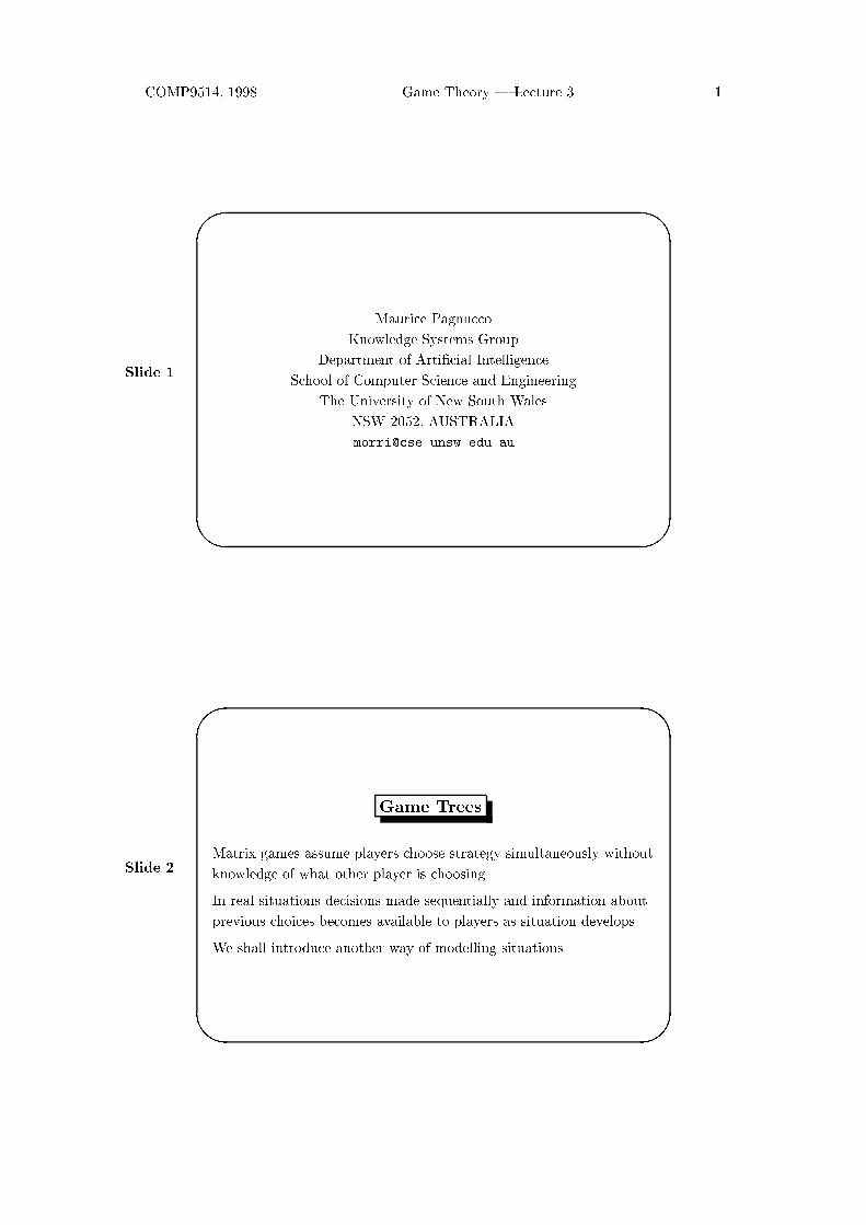
Example (Stra�n 1993, p. 38)

Two players start by putting $1 in the pot. Each player is dealt one

card from a deck of aces and kings. Player 2 must either bet $2 to

continue or drop their hand letting Player 1 win the pot. If Player 2

bets, Player 1 must either call by matching Player 1's bet or fold. If

Player 1 folds, Player 2 wins the pot. If Player 1 calls, the two

players compare cards with the higher card winning or the pot is

split evenly in the case of a draw


Slide 5

'

&

$

%

Chance

P2 P2 P2 P2

K,KK,A

A,K

A,A1/4

1/41/4

1/4

b b b bd d d d

(0,0) (-1,1) (3,-3) (-1,1)

(1,-1)

c f c f c f c f

(1,-1)(1,-1)(1,-1)P1 P1 P1P1

(-3,3) (-1,1) (0,0) (-1,1)

b = bet; d= dropc = call; f = fold

Slide 6

'

&

$

%

Information Sets

In some situations a player may not know where they are in the tree

(e.g., after the deal)

Nodes which represent the player's current situation given the

information at their disposal but are distinct in the tree due to

chance factors form an information set

Nodes in the same information set are linked via dotted lines

(sometimes in the literature circled in dotted regions)


Slide 7

'

&

$

%

Strategy in Game Tree

A strategy (action) in a game tree corresponds to a player's complete

description of choice to be made at any information set in the tree

Knowing strategies of players we can determine course of play

(except for Chance)

Knowing Chance's probabilities we can calculate expected payo�s

Mapping Game Tree to Game Matrix

1. label rows and columns of matrix with players' possible strategies

2. place expected payo�s in entries of matrix

However, number of strategies may be enormous!

Slide 8

'

&

$

%

Continuing Stra�n Example

Examine strategy where Player 2 bets only holding an Ace and

Player 1 calls only holding an Ace

Prob Hands (1, 2) Outcome Payo� (to 1)

1

4A, A 2b, 1c 0

1

4A, K 2d 1

1

4K, A 2b, 1f -1

1

4K, K 2d 1

Expected payof = 1

4:0 + 1

4:1 + 1

4:(�1) + 1

4:1 = 1

4

Game matrix:


Slide 9

'

&

$

%

Player 2 bets

Player 1 calls

Always A Only K Only Never

Always 0 � 1

4

5

41

A Only 1

4

1

41 1

K Only � 5

4� 1

2

1

41

Never -1 0 0 1

Slide 10

'

&

$

%

Games of Perfect Information

{ No nodes labelled Chance

{ Information sets all consist of a single code

Chance has no role in the game

Players know all preceding moves

Such games can be analysed by truncation (or tree pruning)


Slide 11

'

&

$

%

Truncation

Start at leaves of game tree.

For all leaves connected by branches to the same node one level

higher up in the tree select the value at that leaf representing the

best choice for the player labelling the node

Delete all leaves of this node and propagate the best value up to the

node

Continue this process all the way to the root of the tree

Slide 12

'

&

$

%

Example

Player 2

Player 1 Player 1

Player 2 Player 2 Player 2 Player 2

1 3 4 5 -1 2 3


Slide 13

'

&

$

%

Games of Perfect Information

Tree truncation is akin to (iterated) removal of dominated strategies

in matrix games to �nd a saddle point

This process will work for any two-person zero-sum games of perfect

information (just follow the truncation procedure)

Therefore, all two-person zero-sum games of perfect information have

a saddle point

(Zermelo 1912) In a �nite game of complete information one of the

two players has a strategy that can force a win no matter what the

other player does

Slide 14

'

&

$

%

Utility Theory

Where do the numbers come from?

How important are they?

How do we assign numbers to outcomes?

Utility theory: science of assigning numbers to particular outcomes so

as to re ect agent's underlying preferences


Slide 15

'

&

$

%

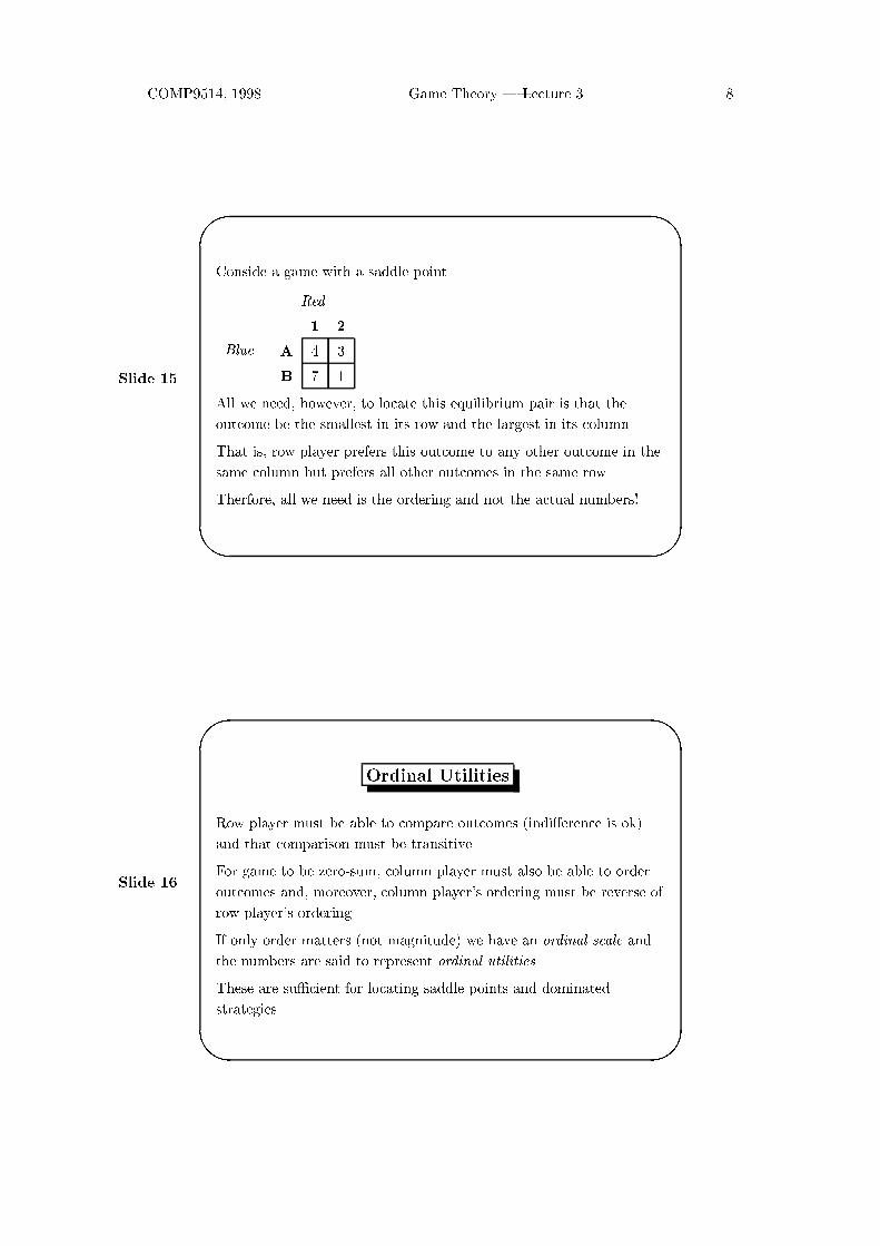
Conside a game with a saddle point

Red

Blue

1 2

A 4 3

B 7 1

All we need, however, to locate this equilibrium pair is that the

outcome be the smallest in its row and the largest in its column

That is, row player prefers this outcome to any other outcome in the

same column but prefers all other outcomes in the same row

Therfore, all we need is the ordering and not the actual numbers!

Slide 16

'

&

$

%

Ordinal Utilities

Row player must be able to compare outcomes (indi�erence is ok)

and that comparison must be transitive

For game to be zero-sum, column player must also be able to order

outcomes and, moreover, column player's ordering must be reverse of

row player's ordering

If only order matters (not magnitude) we have an ordinal scale and

the numbers are said to represent ordinal utilities

These are su�cient for locating saddle points and dominated

strategies


Slide 17

'

&

$

%

Cardinal Utilities

For mixed stratgies, however, we need to calculate ratios.

E.g., using Williams method:

Kershaw

Goldsen

f x Di�s Probs

a -2 4 -6 3

9

i 1 -2 3 6

9

Di�s -3 6

Probs 6

9

3

9

If ratios are important we have an interval (or cardinal) scale and the

numbers are said to be cardinal utilities

Slide 18

'

&

$

%

Ordinals to Cardinals

(von Neumann and Morgenstern)

Suppose an ordering

A < B < C

assign arbitrary numbers to A and C

A = 0; C = 100

Ask question: \is it preferable to have B for certain or a lottery

giving 50% chance of A and 50% chance of C?

If answer is to prefer B, then B is greater than mid-point (50%)

If answer is to prefer lottery, then B is less than mid-point (50%)

Continue using \binary chop"


Slide 19

'

&

$

%

(This is for the row player; for the column player, negate these values

for a zero-sum game.)

Cardinal utilities usually more di�cult to ascertain than ordinal ones

Need cardinal utilities for meaningful mixed-strategy solution! Why?

Slide 20

'

&

$

%

Observation: end points of cardinal utilities are arbitrary

How does this a�ect the choice of numbers?

Di�erent utility assignments represent the same cardinal preferences

as long as there is a positive linear transformation from one to the

other

Positive linear transformation: f(x) = m:x+ b with m > 0 (gradient)

Can transform cardinal utilities by such a function without \altering"

the information they contain


Slide 21

'

&

$

%

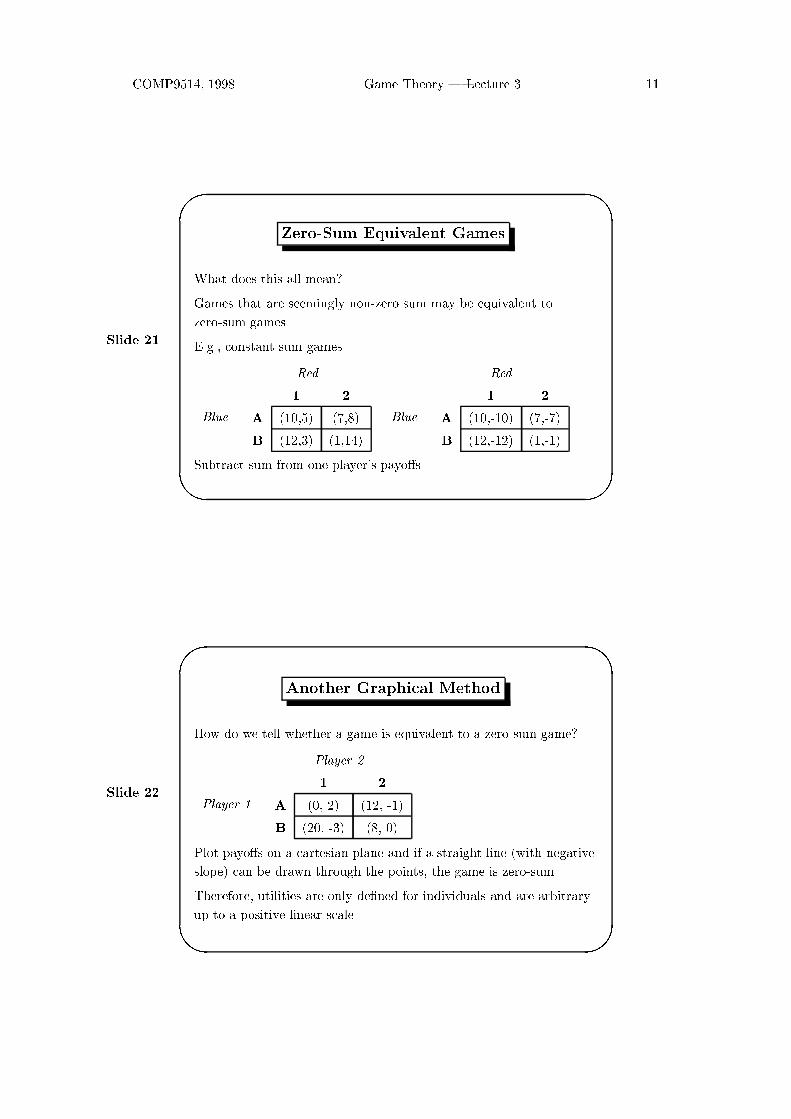
Zero-Sum Equivalent Games

What does this all mean?

Games that are seemingly non-zero sum may be equivalent to

zero-sum games

E.g., constant sum games

Red

Blue

1 2

A (10,5) (7,8)

B (12,3) (1,14)

Red

Blue

1 2

A (10,-10) (7,-7)

B (12,-12) (1,-1)

Subtract sum from one player's payo�s

Slide 22

'

&

$

%

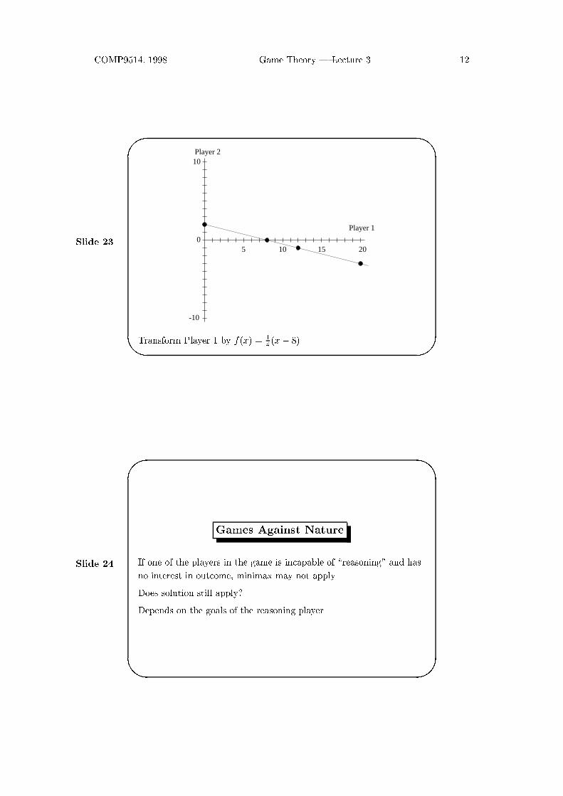
Another Graphical Method

How do we tell whether a game is equivalent to a zero-sum game?

Player 2

Player 1

1 2

A (0, 2) (12, -1)

B (20, -3) (8, 0)

Plot payo�s on a cartesian plane and if a straight line (with negative

slope) can be drawn through the points, the game is zero-sum

Therefore, utilities are only de�ned for individuals and are arbitrary

up to a positive linear scale


Slide 23

'

&

$

%

0

-10

Player 210

Player 1

5 10 15 20

Transform Player 1 by f(x) = 1

4(x � 8)

Slide 24

'

&

$

%

Games Against Nature

If one of the players in the game is incapable of \reasoning" and has

no interest in outcome, minimax may not apply

Does solution still apply?

Depends on the goals of the reasoning player


Slide 25

'

&

$

%

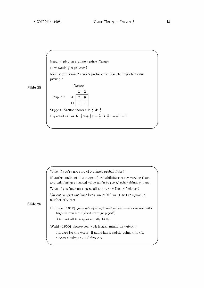
Imagine playing a game against Nature.

How would you proceed?

Idea: if you know Nature's probabilities use the expected value

principle

Nature

Player 1

1 2

A 2 0

B 1 1

Suppose Nature chooses 1: 2

32: 1

3

Expected values A: 2

3:2 + 1

3:0 = 2

3B: 2

3:1 + 1

3:1 = 1

Slide 26

'

&

$

%

What if you're not sure of Nature's probabilities?

If you're con�dent in a range of probabilities can try varying them

and calculating expected value again to see whether things change

What if you have no idea at all about how Nature behaves?

Various suggestions have been made; Milnor (1954) compared a

number of these:

Laplace (1812) principle of insu�cient reason | choose row with

highest sum (or highest average payo�)

Assumes all strategies equally likely

Wald (1950) choose row with largest minimum outcome

Prepare for the worst. If game has a saddle point, this will

choose strategy containing one


Slide 27

'

&

$

%

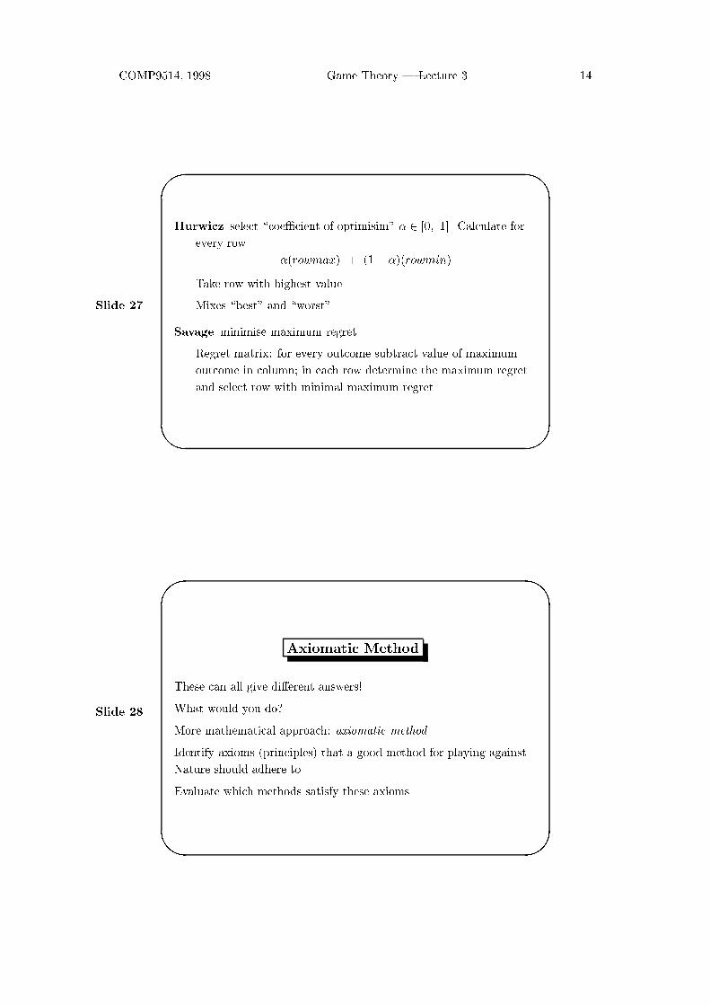
Hurwicz select \coe�cient of optimisim" � 2 [0; 1]. Calculate for

every row

�(rowmax) + (1� �)(rowmin)

Take row with highest value

Mixes \best" and \worst"

Savage minimise maximum regret

Regret matrix: for every outcome subtract value of maximum

outcome in column; in each row determine the maximum regret

and select row with minimal maximum regret

Slide 28

'

&

$

%

Axiomatic Method

These can all give di�erent answers!

What would you do?

More mathematical approach: axiomatic method

Identify axioms (principles) that a good method for playing against

Nature should adhere to

Evaluate which methods satisfy these axioms


Slide 29

'

&

$

%

Axioms

Milnor (1954) suggest the following.

1. ordering: all actions must be completely ordered

2. symmetry: ordering is independent of labelling of rows and

columns

3. strong domination: A is preferred to B if A strongly dominates B

4. linearity: ordering unchanged by linear transformation (all

multiplied by constant or constant added)

5. continuity: If A > B in a sequence of decision problems under

uncertainty, then B 6> A in limiting decision problem under

uncertainty

Slide 30

'

&

$

%

6. column duplication: adding an identical column does not change

ordering

7. column linearity: ordering not changed by adding constant to

column entries

8. row adjunction: ordering between old rows not changed by

adding new rows

9. convexity: If A; B indi�erent in ordering, then neither A nor B

preferred to 1

2A, 1

2B

10. special row adjunction: adding a weakly dominated action does

not change ordering of old actions


Slide 31

'

&

$

%

Comparison of Methods

Axiom Laplace Wald Hurwicz Savage

1. Ordering * * * *

2. Symmetry * * * *

3. Strong domination * * * *

4. Linearity X * * *

5. Continuity X X * X

6. Column duplication * * * {

7. Column linearity * { { *

8. Row adjunction { * * *

9. Convexity X * { *

10. Special row adjunction X X X *

Slide 32

'

&

$

%

(previous slide) * { characterise method; X { method satis�es this

No method satis�es all axioms

Milnor showed these axioms are incompatible!

That is, there can be no method that satisi�es all of them


Slide 33

'

&

$

%

Equilibrium Pair of Strategies

Pair of strategies where player unilaterally deviating from their

equilibrium strategy will worsen their expected payo�.

Minimax theorem implies equilibrium pair and minimax pair coincide

for zero-sum game.

Nash's theorem extends this to non-cooperative games (be they

zero-sum or nonzero-sum).

Slide 34

'

&

$

%

Nonzero-Sum Games

Each player has distinct payo�s which may not be reducible to a

zero-sum game

They may no longer be in direct con ict

They may bene�t from cooperation

Nash's Theorem: Any n-person, noncooperative game (zero-sum

or nonzero-sum) for which each player has a �nite number of pure

strategies has at least one equilibrium set of strategies


Slide 35

'

&

$

%

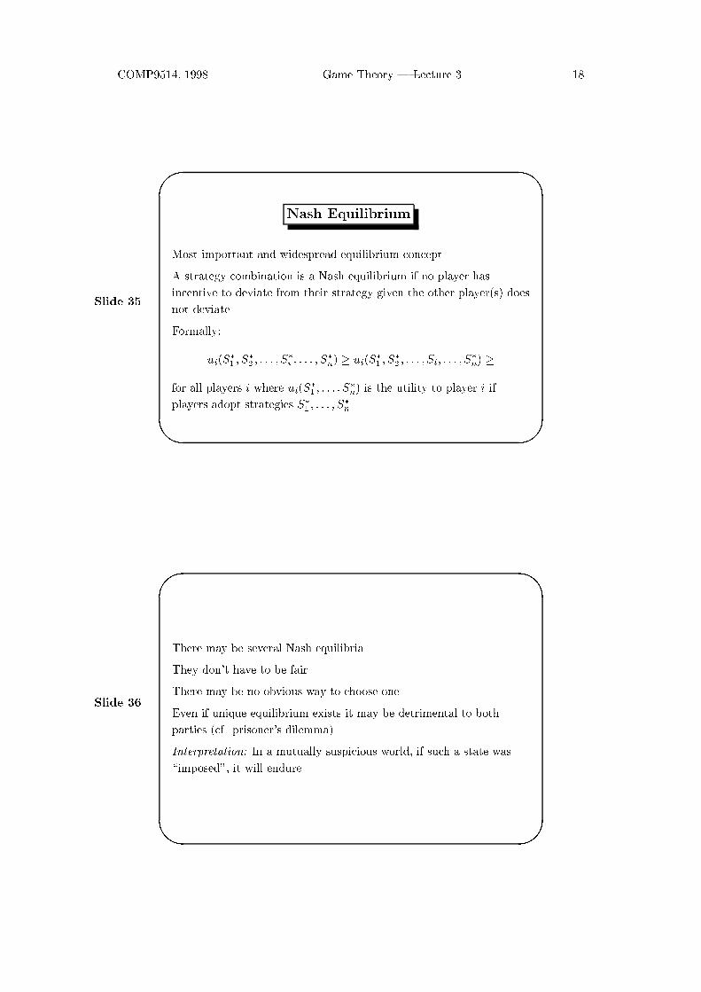
Nash Equilibrium

Most important and widespread equilibrium concept

A strategy combination is a Nash equilibrium if no player has

incentive to deviate from their strategy given the other player(s) does

not deviate

Formally:

ui(S�

1; S�

2; : : : ; S�

i; : : : ; S�

n) � ui(S

�

1; S�

2; : : : ; Si; : : : ; S

�

n) �

for all players i where ui(S�

1; : : : ; S�

n) is the utility to player i if

players adopt strategies S�

1; : : : ; S�

n.

Slide 36

'

&

$

%

There may be several Nash equilibria

They don't have to be fair

There may be no obvious way to choose one

Even if unique equilibrium exists it may be detrimental to both

parties (cf. prisoner's dilemma)

Interpretation: In a mutually suspicious world, if such a state was

\imposed", it will endure


Slide 37

'

&

$

%

Nash Equilibrium

Motivation: dominance implies a chain of reasoning: if Player 1 plays

X , Player 2 plays Y , hence Player 1 should play X 0, then Player 2

should try . . . , then Player 1 might . . .

The hope is that the procedure \zeros-in" on a unique strategy for

each player

Reason: looking for a stable state | equilibrium | where no player

would want to deviate

Slide 38

'

&

$

%

Finding Pure Strategy Nash Equilibria

In two player games:

{ for each strategy of opponent, underline own best reply

{ a cell with both entries underlined represents a (pure-strategy)

Nash Equilibrium

E.g., prisoner's dilemma

Player 2

Player 1

Loyal Fink

Loyal (-1, -1) (-3, 0)

Fink (0, -3) (-2, -2)

Fink Fink is a (pure-strategy) Nash Equilibrium

As in zero-sum games pure-strategy equilibria don't always exist

Therefore, look for mixed-strategy Nash Equilibria | next week


Slide 39

'

&

$

%

Pareto Optimality

De�nition: An outcome is Pareto optimal if there is no other

outcome which would give both players a higher payo� or would give

one player the same payo� and the other player a higher payo�.

Player 2

Player 1

Loyal Fink

Loyal (-1, -1)� (-3, 0)�

Fink (0, -3)� (-2, -2)

Pareto optimal points are on the north east boundary of the payo�

polygon

Slide 40

'

&

$

%

Payo� Polygon

Player 2

0

-1

-2

-3

-3 -2 -1

Player 1


Slide 41

'

&

$

%

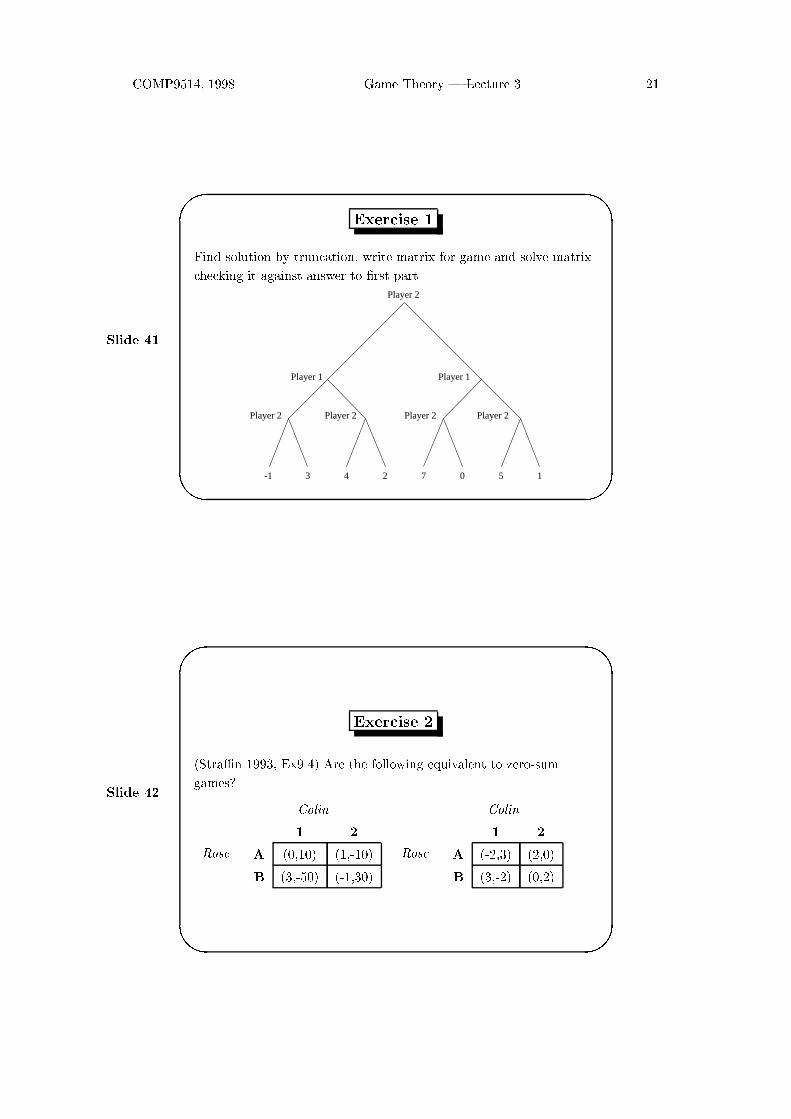
Exercise 1

Find solution by truncation, write matrix for game and solve matrix

checking it against answer to �rst part.

Player 2

Player 1 Player 1

Player 2 Player 2 Player 2 Player 2

-1 3 4 2 7 0 5 1

Slide 42

'

&

$

%

Exercise 2

(Stra�n 1993, Ex9.4) Are the following equivalent to zero-sum

games?

Colin

Rose

1 2

A (0,10) (1,-10)

B (3,-50) (-1,30)

Colin

Rose

1 2

A (-2,3) (2,0)

B (3,-2) (0,2)


Slide 43

'

&

$

%

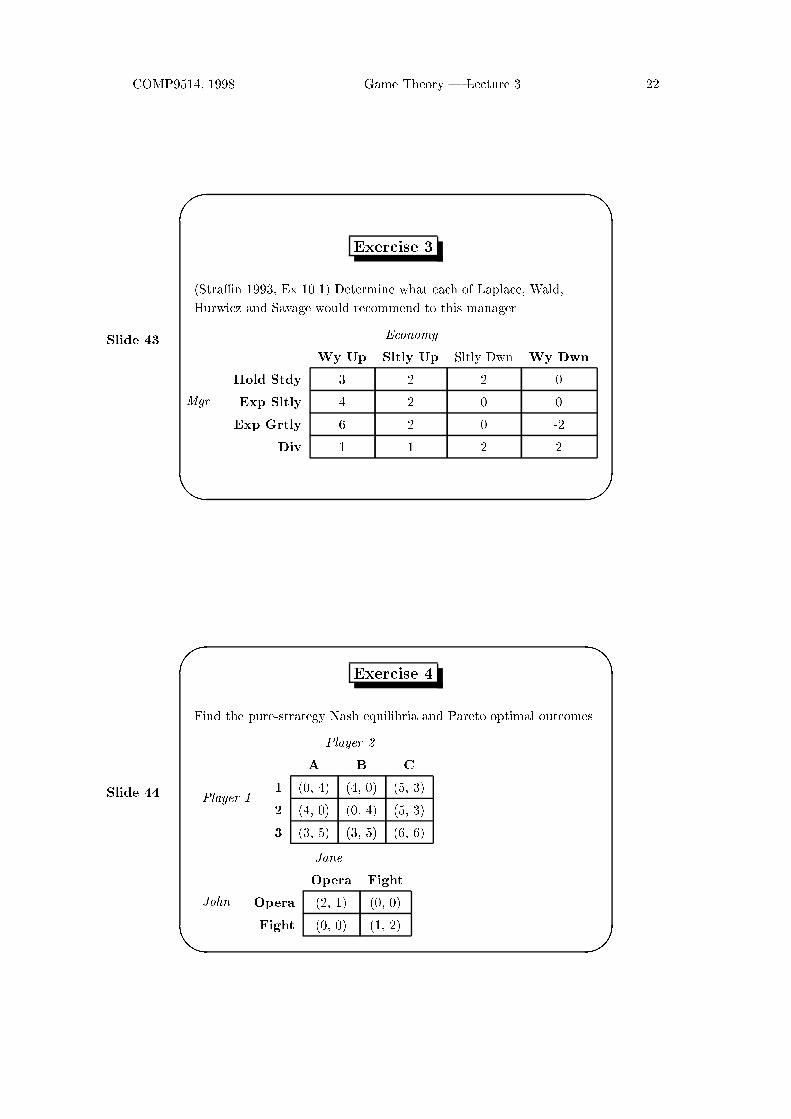
Exercise 3

(Stra�n 1993, Ex 10.1) Determine what each of Laplace, Wald,

Hurwicz and Savage would recommend to this manager.

Economy

Mgr

Wy Up Sltly Up Sltly Dwn Wy Dwn

Hold Stdy 3 2 2 0

Exp Sltly 4 2 0 0

Exp Grtly 6 2 0 -2

Div 1 1 2 2

Slide 44

'

&

$

%

Exercise 4

Find the pure-strategy Nash equilibria and Pareto optimal outcomes

Player 2

Player 1

A B C

1 (0, 4) (4, 0) (5, 3)

2 (4, 0) (0, 4) (5, 3)

3 (3, 5) (3, 5) (6, 6)

Jane

John

Opera Fight

Opera (2, 1) (0, 0)

Fight (0, 0) (1, 2)

Game Theory | Lecture 3morri/comp9514/lecture3.pdf · Game Theory | Lecture 3 9 Slide 17 ' & $ %...

Documents

Transcript of Game Theory | Lecture 3morri/comp9514/lecture3.pdf · Game Theory | Lecture 3 9 Slide 17 ' & $ %...