Game Theory:Dominance, Nash Equilibrium, Symmetry

Branislav L. SlantchevDepartment of Political Science, University of California – San Diego

June 3, 2005

Contents.

1 Elimination of Dominated Strategies 21.1 Strict Dominance in Pure Strategies . . . . . . . . . . . . . . . . . . . . . . . . . . . . 21.2 Weak Dominance . . . . . . . . . . . . . . . . . . . . . . . . . . . . . . . . . . . . . . . . 41.3 Strict Dominance and Mixed Strategies . . . . . . . . . . . . . . . . . . . . . . . . . . 5

2 Nash Equilibrium 82.1 Pure-Strategy Nash Equilibrium . . . . . . . . . . . . . . . . . . . . . . . . . . . . . . . 8

2.1.1 Diving Money . . . . . . . . . . . . . . . . . . . . . . . . . . . . . . . . . . . . . . 102.1.2 The Partnership Game . . . . . . . . . . . . . . . . . . . . . . . . . . . . . . . . 112.1.3 Modified Partnership Game . . . . . . . . . . . . . . . . . . . . . . . . . . . . . 12

2.2 Strict Nash Equilibrium . . . . . . . . . . . . . . . . . . . . . . . . . . . . . . . . . . . . 122.3 Mixed Strategy Nash Equilibrium . . . . . . . . . . . . . . . . . . . . . . . . . . . . . . 13

2.3.1 Battle of the Sexes . . . . . . . . . . . . . . . . . . . . . . . . . . . . . . . . . . . 152.4 Computing Nash Equilibria . . . . . . . . . . . . . . . . . . . . . . . . . . . . . . . . . 17

2.4.1 Myerson’s Card Game . . . . . . . . . . . . . . . . . . . . . . . . . . . . . . . . . 192.4.2 Another Simple Game . . . . . . . . . . . . . . . . . . . . . . . . . . . . . . . . 202.4.3 Choosing Numbers . . . . . . . . . . . . . . . . . . . . . . . . . . . . . . . . . . 212.4.4 Defending Territory . . . . . . . . . . . . . . . . . . . . . . . . . . . . . . . . . . 232.4.5 Choosing Two-Thirds of the Average . . . . . . . . . . . . . . . . . . . . . . . 242.4.6 Voting for Candidates . . . . . . . . . . . . . . . . . . . . . . . . . . . . . . . . 25

3 Symmetric Games 263.1 Heartless New Yorkers . . . . . . . . . . . . . . . . . . . . . . . . . . . . . . . . . . . . 273.2 Rock, Paper, Scissors . . . . . . . . . . . . . . . . . . . . . . . . . . . . . . . . . . . . . 28

4 Strictly Competitive Games 30

5 Five Interpretations of Mixed Strategies 315.1 Deliberate Randomization . . . . . . . . . . . . . . . . . . . . . . . . . . . . . . . . . . 315.2 Equilibrium as a Steady State . . . . . . . . . . . . . . . . . . . . . . . . . . . . . . . . 315.3 Pure Strategies in an Extended Game . . . . . . . . . . . . . . . . . . . . . . . . . . . 325.4 Pure Strategies in a Perturbed Game . . . . . . . . . . . . . . . . . . . . . . . . . . . . 325.5 Beliefs . . . . . . . . . . . . . . . . . . . . . . . . . . . . . . . . . . . . . . . . . . . . . . 32

6 The Fundamental Theorem (Nash, 1950) 32

1 Elimination of Dominated Strategies

1.1 Strict Dominance in Pure Strategies

In some games, a player’s strategy is superior to all other strategies regardless of what theother players do. This strategy then strictly dominates the other strategies. Consider thePrisoner’s Dilemma game in Fig. 1 (p. 2). Choosing D strictly dominates choosing C becauseit yields a better payoff regardless of what the other player chooses to do.

If one player is going to play D, then the other is better off by playing D as well. Also, if oneplayer is going to play C , then the other is better off by playing D again. For each prisoner,choosing D is always better than C regardless of what the other prisoner does. We say thatD strictly dominates C .

Prisoner 1

Prisoner 2C D

C 2,2 0,3D 3,0 1,1

Figure 1: Prisoner’s Dilemma.

Definition 1. In the strategic form game G, let s′i , s′′i ∈ Si be two strategies for player i.

Strategy s′i strictly dominates strategy s′′i if

ui(s′i , s−i) > ui(s′′i , s−i)

for every strategy profile s−i ∈ S−i.In words, a strategy s′i strictly dominates s′′i if for each feasible combination of the other

players’ strategies, i’s payoff from playing s′i is strictly greater than the payoff from playings′′i . Also, strategy s′′i is strictly dominated by s′i . In the PD game, Defect strictly dominatesCooperate, and Cooperate is strictly dominated by Defect.

Rational players never play strictly dominated strategies, because such strategies can neverbe best responses to any strategies of the other players. There is no belief that a rationalplayer can have about the behavior of other players such that it would be optimal to choose astrictly dominated strategy. Thus, in PD a rational player would never choose C . We can usethis concept to find solutions to some simple games. For example, since neither player willever choose C in PD, we can eliminate this strategy from the strategy space, which meansthat now both players only have one strategy left to them: D. The solution is now trivial: Itfollows that the only possible rational outcome is 〈D,D〉.

Because players would never choose strictly dominated strategies, eliminating them fromconsideration should not affect the analysis of the game because this fact should be evi-dent to all players in the game. In the PD example, eliminating strictly dominated strategiesresulted in a unique prediction for how the game is going to be played. The concept ismore general, however, because even in games with more strategies, eliminating a strictlydominated one may result in other strategies becoming strictly dominated in the game thatremains.

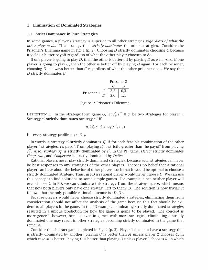
Consider the abstract game depicted in Fig. 2 (p. 3). Player 1 does not have a strategy thatis strictly dominated by another: playing U is better than M unless player 2 chooses C , inwhich caseM is better. Playing D is better than playing U unless player 2 chooses R, in which

2

case U is better. Finally, playing D instead of M is better unless player 2 chooses R, in whichcase M is better.

Player 1

Player 2L C R

U 4,3 5,1 6,2M 2,1 8,4 3,6D 5,9 9,6 2,8

Figure 2: A 3× 3 Example Game.

For player 2, on the other hand, strategy C is strictly dominated by strategy R. Notice thatwhatever player 1 chooses, player 2 is better off playing R than playing C : she gets 2 > 1if player 1 chooses U ; she gets 6 > 4 if player 1 chooses M ; and she gets 8 > 6 if player 1chooses D. Thus, a rational player 2 would never choose to play C when R is available. (Notehere that R neither dominates, nor is dominated by, L.) If player 1 knows that player 2 isrational, then player 1 would play the game as if it were the game depicted in Fig. 3 (p. 3).

Player 1

Player 2L R

U 4,3 6,2M 2,1 3,6D 5,9 2,8

Figure 3: The Reduced Example Game, Step I.

We examine player 1’s strategies again. We now see that U strictly dominates M becauseplayer 1 gets 4 > 2 if player 2 chooses L, and 6 > 3 if player 2 chooses R. Thus, a ra-tional player 1 would never choose M given that he knows player 2 is rational as well andconsequently will never play C . (Note that U neither dominates, nor is dominated by, D.)

If player 2 knows that player 1 is rational and knows that player 1 knows that she is alsorational, then player 2 would play the game as if it were the game depicted in Fig. 4 (p. 3).

Player 1

Player 2L R

U 4,3 6,2D 5,9 2,8

Figure 4: The Reduced Example Game, Step II.

We examine player 2’s strategies again and notice that L now strictly dominates R becauseplayer 2 would get 3 > 2 if player 1 chooses U , and 9 > 8 if player 1 chooses D. Thus, arational player 2 would never choose R given that she knows that player 1 is rational, etc.

If player 1 knows that player 2 is rational, etc., then he would play the game as if it werethe game depicted in Fig. 5 (p. 4).

But now, U is strictly dominated by D, so player 1 would never play U . Therefore, player1’s rational choice here is to play D. This means the outcome of this game will be 〈D,L〉,which yields player 1 a payoff of 5 and player 2 a payoff of 9.

The process described above is called iterated elimination of strictly dominated strate-gies. The solution of G is the equilibrium 〈D,L〉, and is sometimes called iterated-dominance

3

Player 1

Player 2L

U 4,3D 5,9

Figure 5: The Reduced Example Game, Step III.

equilibrium, or iterated-dominant strategy equilibrium. The game G is sometimes calleddominance-solvable.

Although the process is intuitively appealing (after all, rational players would never playstrictly dominated strategies), each step of elimination requires a further assumption aboutthe other player’s rationality. Recall that we started by assuming that player 1 knows thatplayer 2 is rational and so she would not play C . This allowed the elimination of M . Next,we had to assume that player 2 knows that player 1 is rational and that she also knows thatplayer 1 knows that she herself is rational as well. This allowed the elimination of R. Finally,we had to assume that player 1 knows that player 2 is rational and that he also knows thatplayer 2 knows that player 1 is rational and that player 2 also knows that player 1 knows thatplayer 2 is rational.

More generally, we want to be able to make this assumption for as many iterations as mightbe needed. That is, we must be able to assume not only that all players are rational, but alsothat all players know that all the players are rational, and that all the players know that allthe players know that all players are rational, and so on, ad infinitum. This assumption iscalled common knowledge and is usually made in game theory.

1.2 Weak Dominance

Rational players would never play strictly dominated strategies, and so eliminating theseshould not affect our analysis. There may be circumstances, however, where a strategy is“not worse” than another instead of being “always better” (as a strictly dominant one wouldbe). To define this concept, we introduce the idea of weakly dominated strategy.

Definition 2. In the strategic form game G, let s′i , s′′i ∈ Si be two strategies for player i.

Strategy s′i weakly dominates strategy s′′i if

ui(s′i , s−i) ≥ ui(s′′i , s−i)

for every strategy profile s−i ∈ S−i, and there exists at least one s−i such that the inequalityis strict.

In other words, s′i never does worse than s′′i , and sometimes does better. While iteratedelimination of strictly dominated strategies seems to rest on rather firm foundation (exceptfor the common knowledge requirement that might be a problem with more complicated situ-ations), eliminating weakly dominated strategies is more controversial because it is harder toargue that it should not affect analysis. The reason is that by definition, a weakly dominatedstrategy can be a best response for the player. Furthermore, there are technical difficultieswith eliminating weakly dominated strategies: the order of elimination can matter for theresult!

Consider the game in Fig. 6 (p. 5). Strategy D is strictly dominated by U , so if we removeit first, we are left with a game, in which L weakly dominates R. Eliminating R in turn results

4

Player 1

Player 2L R

U 3,2 2,2M 1,1 0,0D 0,0 1,1

Figure 6: The Kohlberg and Mertens Game.

in a game where U strictly dominates M , and so the prediction is 〈U,L〉. However, note thatM is strictly dominated by U in the original game as well. If we begin by eliminating M , thenR weakly dominates L in the resulting game. Eliminating L in turn results in a game whereU strictly dominates D, and so the prediction is 〈U,R〉. If we begin by eliminating M and Dat the same time, then we are left with a game where neither of the strategies for player 2weakly dominates the other. Thus, the order in which we eliminate the strictly dominatedstrategies for player 1 determines which of player 2’s weakly dominated strategies will geteliminated in the iterative process.

This dependence on the order of elimination does not arise if we only eliminated strictlydominated strategies. If we perform the iterative process until no strictly dominated strate-gies remain, the resulting game will be the same regardless of the order in which we performthe elimination. Eliminating strategies for other players can never cause a strictly dominatedstrategy to cease to be dominated but it can cause a weakly dominated strategy to cease be-ing dominated. Intuitively, you should see why the latter might be the case. For a strategy sito be weakly dominated, all that is required is that some other strategy s′i is as good as si forall strategies s−i and only better than si for one strategy of the opponent. If that particularstrategy gets eliminated, then si and s′i yield the same payoffs for all remaining strategies ofthe opponent, and neither weakly dominates the other.

1.3 Strict Dominance and Mixed Strategies

We now generalize the idea of dominance to mixed strategies. All that we have to do to decidewhether a pure strategy is dominated is to check whether there exists some mixed-strategythat is a better response to all pure strategies of the opponents.

Definition 3. In a strategic form game G with vNM preferences, the pure strategy si isstrictly dominated for player i if there exists a mixed strategy σi ∈ Σi such that

ui(σi, s−i) > ui(si, s−i) for every s−i ∈ S−i. (1)

The strategy si is weakly dominated if there exists a σi such that inequality (1) holds withweak inequality, and the inequality is strict for at least one s−i.

Note that when checking if a pure strategy is dominated by a mixed strategy, we onlyconsider pure strategies for the rest of the players. This is because for a given si, the strategyσi satisfies (1) for all pure strategies of the opponents if, and only if, it satisfies it for all mixedstrategies σ−i as well because player i’s payoff when his opponents play mixed strategies isa convex combination of his payoffs when they play pure strategies.

As a first example of a pure strategy dominated by a mixed strategy, consider our favoritecard game, whose strategic form, reproduced in Fig. 7 (p. 6), we have derived before. Consider

5

strategy s1 = Ff for player 1 and the mixed strategy σ1 = (0.5)[Rr] + (0.5)[Fr]. We nowhave:

u1(σ1,m) = (0.5)(0)+ (0.5)(0.5) = 0.25 > 0 = u1(s1,m)u1(σ1, p) = (0.5)(1)+ (0.5)(0) = 0.5 > 0 = u1(s1, p).

In other words, playing σ1 yields a higher expected payoff than s1 does against any possiblestrategy for player 2. Therefore, s1 is strictly dominated by σ1, and we should not expectplayer 1 to play s1. On the other hand, the strategy Fr only weakly dominates Ff becauseit yields a strictly better payoff against m but the same payoff against p. Eliminating weaklydominated strategies is much more controversial than eliminating strictly dominated ones(we shall see why in the homework).

Player 1

Player 2m p

Rr 0,0 1,−1Rf −0.5,0.5 1,−1Fr 0.5,−0.5 0,0Ff 0,0 0,0

Figure 7: The Strategic Form of the Myerson Card Game.

As an example of iterated elimination of strictly dominated strategies that can involvemixed strategies, consider the game in Fig. 8 (p. 6). None of the pure strategies for player 1strictly dominates any of his other strategies. Further, no mixed strategy for player 1 strictlydominates any of his pure strategies. This is easy to see: since U is a best response to C ,it cannot be dominated by any mixed strategy that assigns positive probability to D becausesuch a strategy would yield a strictly lower payoff against C . A similar argument establishesthat D cannot be dominated by any mixed strategy because D is a best response to R.

Player 1

Player 2L C R

U 2,3 3,0 0,1D 0,0 1,6 4,2

Figure 8: Another Game from Myerson (p. 58).

Further, none of the pure strategies strictly dominates any other strategy for player 2.Let’s see if we can find a mixed strategy for player 2 that would strictly dominate one of herpure strategies. Which pure strategy should we try to eliminate? It cannot be C because anymixture between L and R would involve a convex combination of 0 and 2 against D whichcan never exceed 6, which is what C would yield in this case. It cannot be L either because ityields 3 against U , and any mixture between C and R against U would yield at most 1. Hence,let’s try to eliminate R: one can imagine mixtures between L and C that would yield a payoffhigher than 1 against U and higher than 2 against D. One such mixture would be playingthem both with equal probability. The mixed strategy σ2 = (0.5)[L] + (0.5)[C] = (.5, .5,0)strictly dominates the pure strategy R. To see this, note that

u2(σ2, U) = (0.5)(3)+ (0.5)(0) = 1.5 > 1 = u2(R,U)u2(σ2,D) = (0.5)(0)+ (0.5)(6) = 3 > 2 = u2(R,D).

6

We can therefore eliminate R, which produces the game in Fig. 9 (p. 7).

Player 1

Player 2L C

U 2,3 3,0D 0,0 1,6

Figure 9: The Game from Fig. 8 (p. 6) after Elimination of R.

In this game, strategy U strictly dominates D because 2 > 0 against L and 3 > 1 againstC . Therefore, because player 1 knows that player 2 is rational and would never choose R, hecan eliminate D from his own choice set. But now player 2’s choice is also simple becausein the resulting game L strictly dominates C because 3 > 0. She therefore eliminates thisstrategy from her choice set. The iterated elimination of strictly dominated strategies leadsto a unique prediction as to what rational players should do in this game: 〈U,L〉.

The following several remarks are useful observations about the relationship between dom-inance and mixed strategies. Each is easily verifiable by example.

Remark 1. A mixed strategy that assigns positive probability to a dominated pure strategyis itself dominated (by any other mixed strategy that assigns less probability to the dominatedpure strategy).

Remark 2. A mixed strategy may be strictly dominated even though it assigns positiveprobability only to pure strategies that are not even weakly dominated.

Player 1

Player 2L R

U 1,3 −2,0M −2,0 1,3D 0,1 0,1

Figure 10: Mixed Strategy Dominated by a Pure Strategy.

Consider the example in Fig. 10 (p. 7). Playing U and M with probability 1/2 each givesplayer 1 an expected payoff of −1/2 regardless of what player 2 does. This is strictly domi-nated by the pure strategy D, which gives him a payoff of 0, even though neither U nor M is(even weakly) dominated.

Remark 3. A strategy not strictly dominated by any other pure strategy may be strictlydominated by a mixed strategy.

Player 1

Player 2L R

U 1,3 1,0M 4,0 0,3D 0,1 3,1

Figure 11: Pure Strategy Dominated by a Mixed Strategy.

7

Consider the example in Fig. 11 (p. 7). Playing U is not strictly dominated by either M or Dand gives player 1 a payoff of 1 regardless of what player 2 does. This is strictly dominatedby the mixed strategy in which player 1 chooses M and D with probability 1/2 each, whichwould yield 2 if player 2 chooses L and 3/2 if player 2 chooses R, and so it would yield atleast 3/2 > 1 regardless of what player 2 does.

The iterated elimination of strictly dominated strategies is quite intuitive but it has a veryimportant drawback. Even though the dominant strategy equilibrium is unique if it exists,for most games that we wish to analyze, all strategies (or too many of them) will surviveiterated elimination, and there will be no such equilibrium. Thus, this solution concept willleave many games “unsolvable” in the sense that we shall not be able predict how rationalplayers will play them. In contrast, the concept of Nash equilibrium, to which we turn now,has the advantage that it exists in a very broad class of games.

2 Nash Equilibrium

2.1 Pure-Strategy Nash Equilibrium

Rational players think about actions that the other players might take. In other words, playersform beliefs about one another’s behavior. For example, in the BoS game, if the man believedthe woman would go to the ballet, it would be prudent for him to go to the ballet as well.Conversely, if he believed that the woman would go to the fight, it is probably best if he wentto the fight as well. So, to maximize his payoff, he would select the strategy that yields thegreatest expected payoff given his belief. Such a strategy is called a best response (or bestreply).

Definition 4. Suppose player i has some belief s−i ∈ S−i about the strategies played by theother players. Player i’s strategy si ∈ Si is a best response if

ui(si, s−i) ≥ ui(s′i , s−i) for every s′i ∈ Si.

We now define the best response correspondence), BRi(s−i), as the set of best responsesplayer i has to s−i. It is important to note that the best response correspondence is set-valued. That is, there may be more than one best response for any given belief of player i. Ifthe other players stick to s−i, then player i can do no better than using any of the strategiesin the set BRi(s−i). In the BoS game, the set consists of a single member: BRm(F) = {F} andBRm(B) = {B}. Thus, here the players have a single optimal strategy for every belief. In othergames, like the one in Fig. 12 (p. 8), BRi(s−i) can contain more than one strategy.

Player 1

Player 2L C R

U 2,2 1,4 4,4M 3,3 1,0 1,5D 1,1 0,5 2,3

Figure 12: The Best Response Game.

In this game, BR1(L) = {M}, BR1(C) = {U,M}, and BR1(R) = {U}. Also, BR2(U) = {C,R},BR2(M) = {R}, and BR2(D) = {C}. You should get used to thinking of the best response cor-respondence as a set of strategies, one for each combination of the other players’ strategies.

8

(This is why we enclose the values of the correspondence in braces even when there is onlyone element.)

We can now use the concept of best responses to define Nash equilibrium: a Nash equi-librium is a strategy profile such that each player’s strategy is a best response to the otherplayers’ strategies:

Definition 5 (Nash Equilibrium). The strategy profile (s∗i , s∗−i) ∈ S is a pure-strategy Nash

equilibrium if, and only if, s∗i ∈ BRi(s∗−i) for each player i ∈ I .An equivalent useful way of defining Nash equilibrium is in terms of the payoffs players

receive from various strategy profiles.

Definition 6. The strategy profile (s∗i , s∗−i) is a pure-strategy Nash equilibrium if, and only

if, ui(s∗i , s∗−i) ≥ ui(si, s∗−i) for each player i ∈ I and each si ∈ Si.

That is, for every player i and every strategy si of that player, (s∗i , s∗−i) is at least as good

as the profile (si, s∗−i) in which player i chooses si and every other player chooses s∗−i. In aNash equilibrium, no player i has an incentive to choose a different strategy when everyoneelse plays the strategies prescribed by the equilibrium. It is quite important to understandthat a strategy profile is a Nash equilibrium if no player has incentive to deviate fromhis strategy given that the other players do not deviate. When examining a strategy for acandidate to be part of a Nash equilibrium (strategy profile), we always hold the strategies ofall other players constant.1

To understand the definition of Nash equilibrium a little better, suppose there is someplayer i, for whom si is not a best response to s−i. Then, there exists some s′i such thatui(s′i , s−i) > ui(si, s−i). Then this (at least one) player has an incentive to deviate from thetheory’s prediction and these strategies are not Nash equilibrium.

Another important thing to keep in mind: Nash equilibrium is a strategy profile. Findinga solution to a game involves finding strategy profiles that meet certain rationality require-ments. In strict dominance we required that neither of the player’s strategies in equilibriumis strictly dominated. In Nash equilibrium, we require that each player’s strategy is a bestresponse to the strategies of the other players.

The Prisoners’ Dilemma. By examining all four possible strategy profiles, we see that (D,D)is the unique Nash equilibrium (NE). It is NE because (a) given that player 2 chooses D, thenplayer 1 can do no better than chose D himself (1 > 0); and (b) given that player 1 choosesD, player 2 can do no better than choose D himself. No other strategy profile is NE:

• (C,C) is not NE because if player 2 chooses C , then player 1 can profitably deviate bychoosing D (3 > 2). Although this is enough to establish the claim, also note that theprofile is not NE for another sufficient reason: if player 1 chooses C , then player 2 canprofitably deviate by playing D instead. (Note that it is enough to show that one playercan deviate profitably for a profile to be eliminated.)

• (C,D) is not NE because if player 2 chooses D, then player 1 can get a better payoff bychoosing D as well.

1There are several ways to motivate Nash equilibrium. Osborne offers the idea of social convention andGibbons justifies it on the basis of self-enforcing predictions. Each has its merits and there are others (e.g.steady state in an evolutionary game). You should become familiar with these.

9

• (D,C) is not NE because if player 1 chooses D, then player 2 can get a better payoff bychoosing D as well.

Since this exhausts all possible strategy profiles, (D,D) is the unique Nash equilibrium ofthe game. It is no coincidence that the Nash equilibrium is the same as the strict dominanceequilibrium we found before. In fact, as you will have to prove in your homework, a playerwill never use a strictly dominated strategy in a Nash equilibrium. Further, if a game isdominance solvable, then its solution is the unique Nash equilibrium.

How do we use best responses to find Nash equilibria? We proceed in two steps: First, wedetermine the best responses of each player, and second, we find the strategy profiles wherestrategies are best responses to each other.

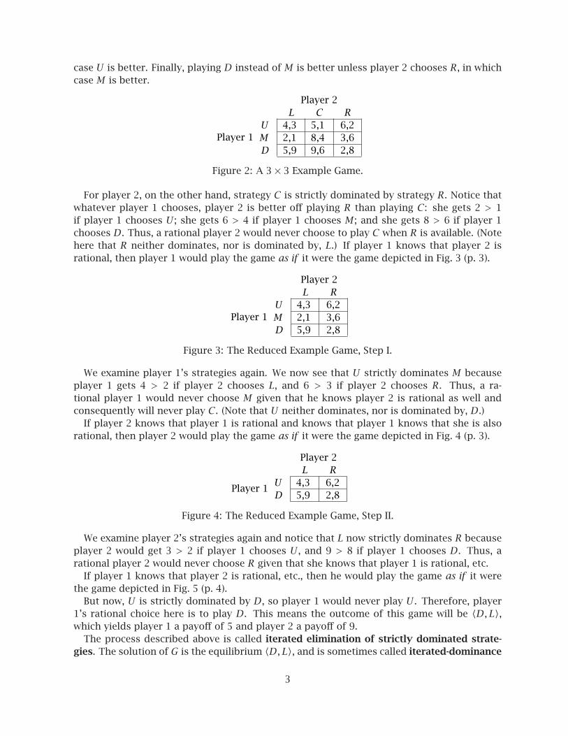
For example, consider again the game in Fig. 12 (p. 8). We have already determined the bestresponses for both players, so we only need to find the profiles where each is best responseto the other. An easy way to do this in the bi-matrix is by going through the list of bestresponses and marking the payoffs with a ’*’ for the relevant player where a profile involvesa best response. Thus, we mark player 1’s payoffs in (U,C), (U,R), (M,L), and (M,C). Wealso mark player 2’s payoffs in (U,C), (U,R), (M,R), and (D,C). This yields the matrix inFig. 13 (p. 10).

Player 1

Player 2L C R

U 2,2 1*,4* 4*,4*M 3*,3 1*,0 1,5*D 1,1 0,5* 2,3

Figure 13: The Best Response Game Marked.

There are two profiles with stars for both players, (U,C) and (U,R), which means theseprofiles meet the requirements for NE. Thus, we conclude this game has two pure-strategyNash equilibria.

2.1.1 Diving Money

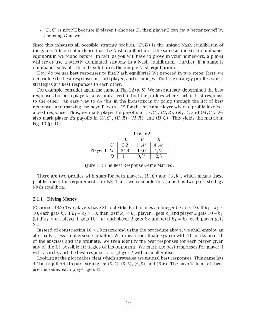
(Osborne, 38.2) Two players have $1 to divide. Each names an integer 0 ≤ k ≤ 10. If k1+k2 ≤10, each gets ki. If k1+k2 > 10, then (a) if k1 < k2, player 1 gets k1 and player 2 gets 10−k1;(b) if k1 > k2, player 1 gets 10 − k2 and player 2 gets k2; and (c) if k1 = k2, each player gets$5.

Instead of constructing 10× 10 matrix and using the procedure above, we shall employ analternative, less cumbersome notation. We draw a coordinate system with 11 marks on eachof the abscissa and the ordinate. We then identify the best responses for each player givenany of the 11 possible strategies of his opponent. We mark the best responses for player 1with a circle, and the best responses for player 2 with a smaller disc.

Looking at the plot makes clear which strategies are mutual best responses. This game has4 Nash equilibria in pure strategies: (5,5), (5,6), (6,5), and (6,6). The payoffs in all of theseare the same: each player gets $5.

10

s2

s10 1 2 3 4 5 6 7 8 9 10

0

1

2

3

4

5

6

7

8

9

10

�

�

�

�

�

�

�

�

�

�

�

�

�

�

�

�

�

�

�

��

� �

�

�

�

�� � � � � �

� � � � �

� � � �

� � �

� �

� �

� �

�

�

�

Figure 14: Best Responses in the Dividing Money Game.

2.1.2 The Partnership Game

There is a firm with two partners. The firm’s profit depends on the effort each partner ex-pends on the job and is given by p = 4(x+y+cxy), where x is the amount of effort expendedby partner 1 and y is the amount of effort expended by partner 2. Assume that x,y ∈ [0,4].The value c ∈ [0, 1/4] measures how complementary the tasks of the partners are. Partner1 incurs a personal cost x2 of expending effort, and partner 2 incurs cost y2. Each partnerselects the level of his effort independently of the other, and both do so simultaneously. Eachpartner seeks to maximize their share of the firm’s profit (which is split equally) net of thecost of effort. That is, the payoff function for partner 1 is u1(x,y) = p/2− x2, and that forpartner 2 is u2(x,y) = p/2−y2.

The strategy spaces here are continuous and we cannot construct a payoff matrix. (Math-ematically, S1 = S2 = [0,4] and �S = [0,4] × [0,4].) We can, however, analyze this gameusing best response functions. Let y represent some belief partner 1 has about the otherpartner’s effort. In this case, partner 1’s payoff will be 2(x + y + cxy) − x2. We need tomaximize this expression with respect to x (recall that we are holding partner’s two strategyconstant and trying to find the optimal response for partner 1 to that strategy). Taking thederivative yields 2 + 2cy − 2x. Setting the derivative to 0 and solving for x yields the bestresponse BR1(y) = {1+cy}. Going through the equivalent calculations for the other partneryields his best response function BR2(x) = {1+ cx}.

We are now looking for a strategy profile (x∗, y∗) such that x∗ = BR1(y∗) and y∗ =BR2(x∗). (We can use equalities here because the best response functions produce singlevalues!) To find this profile, we solve the system of equations:

x∗ = 1+ cy∗y∗ = 1+ cx∗.

The solution is x∗ = y∗ = 1/(1− c). Thus, this game has a unique Nash equilibrium in pure

11

strategies, in which both partners expend 1/(1− c) worth of effort.

2.1.3 Modified Partnership Game

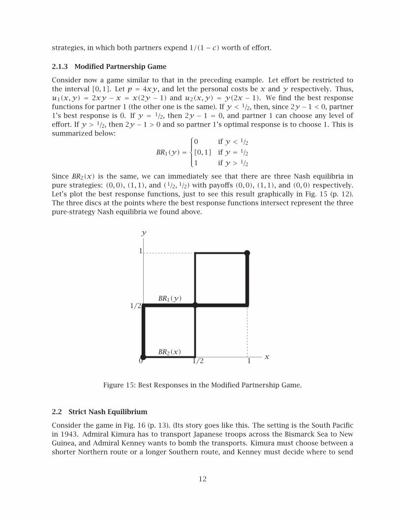
Consider now a game similar to that in the preceding example. Let effort be restricted tothe interval [0,1]. Let p = 4xy , and let the personal costs be x and y respectively. Thus,u1(x,y) = 2xy − x = x(2y − 1) and u2(x,y) = y(2x − 1). We find the best responsefunctions for partner 1 (the other one is the same). If y < 1/2, then, since 2y −1 < 0, partner1’s best response is 0. If y = 1/2, then 2y − 1 = 0, and partner 1 can choose any level ofeffort. If y > 1/2, then 2y − 1 > 0 and so partner 1’s optimal response is to choose 1. This issummarized below:

BR1(y) =

⎧⎪⎪⎨⎪⎪⎩

0 if y < 1/2[0,1] if y = 1/21 if y > 1/2

Since BR2(x) is the same, we can immediately see that there are three Nash equilibria inpure strategies: (0,0), (1,1), and (1/2, 1/2) with payoffs (0,0), (1,1), and (0,0) respectively.Let’s plot the best response functions, just to see this result graphically in Fig. 15 (p. 12).The three discs at the points where the best response functions intersect represent the threepure-strategy Nash equilibria we found above.

y

x0 1

1

1/2

1/2

�

�

�

BR1(y)

BR2(x)

Figure 15: Best Responses in the Modified Partnership Game.

2.2 Strict Nash Equilibrium

Consider the game in Fig. 16 (p. 13). (Its story goes like this. The setting is the South Pacificin 1943. Admiral Kimura has to transport Japanese troops across the Bismarck Sea to NewGuinea, and Admiral Kenney wants to bomb the transports. Kimura must choose between ashorter Northern route or a longer Southern route, and Kenney must decide where to send

12

his planes to look for the transports. If Kenney sends the plans to the wrong route, he canrecall them, but the number of days of bombing is reduced.)

Kenney

KimuraN S

N 2,-2 2,-2S 1,-1 3,-3

Figure 16: The Battle of Bismarck Sea.

This game has a unique Nash equilibrium, in which both choose the northern route, (N,N).Note, however, that if Kenney plays N, then Kimura is indifferent between N and S (becausethe advantage of the shorter route is offset by the disadvantage of longer bombing raids).Still, the strategy profile (N,N) meets the requirements of NE. This equilibrium is not strict.

More generally, an equilibrium is strict if, and only if, each player has a unique best re-sponse to the other players’ strategies:

Definition 7. A strategy profile (s∗i , s∗−i) is a strict Nash equilibrium if for every player i,

ui(s∗i , s∗−i) > ui(si, s

∗−i) for every strategy si ≠ s∗i .

The difference from the original definition of NE is only in the strict inequality sign.

2.3 Mixed Strategy Nash Equilibrium

The most common example of a game with no Nash equilibrium in pure strategies is Match-ing Pennies, which is given in Fig. 17 (p. 13).

Player 1

Player 2H T

H 1,−1 −1,1T −1,1 1,−1

Figure 17: Matching Pennies.

This is a strictly competitive (zero-sum) situation, in which the gain for one player is theloss of the other.2 This game has no Nash equilibrium in pure strategies. Let’s considermixed strategies.

We first extend the idea of best responses to mixed strategies: Let BRi(σ−i) denote playeri’s best response correspondence when the others play σ−i. The definition of Nash equilib-rium is analogous to the pure-strategy case:

Definition 8. A mixed strategy profile σ∗ is a mixed-strategy Nash equilibrium if, andonly if, σ∗i ∈ BRi(σ∗−i).

As before, a strategy profile is a Nash equilibrium whenever all players’ strategies are bestresponses to each other. For a mixed strategy to be a best response, it must put positiveprobabilities only on pure strategies that are best responses. Mixed strategy equilibria, likepure strategy equilibria, never use dominated strategies.

2It is these zero-sum games that von Neumann and Morgenstern studied and found solutions for. However,Nash’s solution can be used in non-zero-sum games, and is thus far more general and useful.

13

Turning now to Matching Pennies, let σ1 = (p,1 − p) denote a mixed strategy for player1 where he chooses H with probability p, and T with probability 1 − p. Similarly, let σ2 =(q,1− q) denote a mixed strategy for player 2 where she chooses H with probability q, andT with probability 1− q. We now derive the best response correspondence for player 1 as afunction of player 2’s mixed strategy.

Player 1’s expected payoffs from his pure strategies given player 2’s mixed strategy are:

u1(H,σ2) = (1)q + (−1)(1− q) = 2q − 1

u1(T ,σ2) = (−1)q + (1)(1− q) = 1− 2q.

Playing H is a best response if, and only if:

u1(H,σ2) ≥ u1(T ,σ2)2q − 1 ≥ 1− 2q

q ≥ 1/2.

Analogously, T is a best response if, and only if, q ≤ 1/2. Thus, player 1 should choose p = 1if q ≥ 0.5 and p = 0 if q ≤ 0.5. Note now that whenever q = 0.5, player 1 is indifferentbetween his two pure strategies: choosing either one yields the same expected payoff of 0.Thus, both strategies are best responses, which implies that any mixed strategy that includesboth of them in its support is a best response as well. Again, the reason is that if the player isgetting the same expected payoff from his two pure strategies, he will get the same expectedpayoff from any mixed strategy whose support they are.

Analogous calculations yield the best response correspondence for player 2 as a functionof σ1. Putting these together yields:

BR1(q) =

⎧⎪⎪⎨⎪⎪⎩

0 if q < 1/2[0,1] if q = 1/21 if q > 1/2

BR2(p) =

⎧⎪⎪⎨⎪⎪⎩

0 if p > 1/2[0,1] if p = 1/21 if p < 1/2

The graphical representation of the best response correspondences is in Fig. 18 (p. 15). Theonly place where the randomizing strategies are best responses to each other is at the in-tersection point, where each player randomizes between the two strategies with probability1/2. Thus, the Matching Pennies game has a unique Nash equilibrium in mixed strategies⟨σ∗1 , σ

∗2

⟩, where σ∗1 = (1/2, 1/2), and σ∗2 = (1/2, 1/2). That is, where p = q = 0.5.

As before, the alternative definition of Nash equilibrium is in terms of the payoff functions.We require that no player can do better by using any other strategy than the one he uses in theequilibrium mixed strategy profile given that all other players stick to their mixed strategies.In other words, the player’s expected payoff of the MSNE profile is at least as good as theexpected payoff of using any other strategy.

Definition 9. A mixed strategy profile σ∗ is a mixed-strategy Nash equilibrium if, for allplayers i,

ui(σ∗i , σ∗−i) ≥ ui(si, σ∗−i) for all si ∈ Si.

Since expected utilities are linear in the probabilities, if a player uses a non-degenerate mixedstrategy in a Nash equilibrium, then he must be indifferent between all pure strategies towhich he assigns positive probability. This is why we only need to check for a profitable purestrategy deviation. (Note that this differs from Osborne’s definition, which involves checkingagainst profitable mixed strategy deviations.)

14

q

p0 1

1

1/2

1/2 �BR1(q)

BR2(p)

Figure 18: Best Responses in Matching Pennies.

2.3.1 Battle of the Sexes

We now analyze the Battle of the Sexes game, reproduced in Fig. 19 (p. 15).

Player 1

Player 2F B

F 2,1 0,0B 0,0 1,2

Figure 19: Battle of the Sexes.

As a first step, we plot each player’s expected payoff from each of the pure strategies asa function of the other player’s mixed strategy. Let p denote the probability that player 1chooses F , and let q denote the probability that player 2 chooses F . Player 1’s expectedpayoff from F is then 2q+0(1−q) = 2q, and his payoff from B is 0q+1(1−q) = 1−q. Since2q = 1− q whenever q = 1/3, the two lines intersect there.

Looking at the plot in Fig. 20 (p. 16) makes it obvious that for any q < 1/3, player 1 has aunique best response in playing the pure strategy B, for q > 1/3, his best response is againunique and it is the pure strategy F , while at q = 1/3, he is indifferent between his two purestrategies, which also implies he will be indifferent between any mixing of them. Thus, wecan specify player 1’s best response (in terms of p):

BR1(q) =

⎧⎪⎪⎨⎪⎪⎩

0 if q < 1/3[0,1] if q = 1/31 if q > 1/3

We now do the same for the expected payoffs of player 2’s pure strategies as a function ofplayer 1’s mixed strategy. Her expected payoff from F is 1p+ 0(1−p) = p and her expected

15

u1(·)

q0 1

2

1/3

1

u1(F, q)

u1(B, q)��

��

��

��

��

��

��

��

����������������

Figure 20: Player 1 Expected Payoffs as a Function of the Player 2s Mixed Strategy.

payoff from B is 0p + 2(1 − p) = 2(1 − p). Noting that p = 2(1 − p) whenever p = 2/3, weshould expect that the plots of her expected payoffs from the pure strategies will intersectat p = 2/3. Indeed, Fig. 21 (p. 16) shows that this is the case.

u2(·)

p0 1

2

2/3

1

u2(p, F)

u2(p, B)

����������������

��

��

��

��

��

��

��

��

Figure 21: Player 2’s Expected Payoffs as a Function of Player 1’s Mixed Strategy.

Looking at the plot reveals that player 2 strictly prefers playing B whenever p < 2/3, strictlyprefers playing F whenever p > 2/3, and is indifferent between the two (and any mixture of

16

them) whenever p = 2/3. This allows us to specify her best response (in terms of q):

BR2(p) =

⎧⎪⎪⎨⎪⎪⎩

0 if p < 2/3[0,1] if p = 2/31 if p > 2/3

q

p0 1

1

2/3

1/3 �

�

�

BR1(q)

BR2(p)

Figure 22: Best Responses in Battle of the Sexes.

Having derived the best response correspondences, we can plot them in the p × q space,which is done in Fig. 22 (p. 17). The best response correspondences intersect in three places,which means there are three mixed strategy profiles in which the two strategies are bestresponses of each other. Two of them are in pure-strategies: the degenerate mixed strategyprofiles 〈1,1〉 and 〈0,0〉. In addition, there is one mixed-strategy equilibrium,

⟨(2/3[F], 1/3[B]) , (1/3[F], 2/3[B])

⟩.

In the mixed strategy equilibrium, each outcome occurs with positive probability. To cal-culate the corresponding probability, multiply the equilibrium probabilities of each playerchoosing the relevant action. This yields Pr(F, F) = 2/3 × 1/3 = 2/9, Pr(B, B) = 1/3 × 2/3 = 2/9,Pr(F, B) = 2/3 × 2/3 = 4/9, and Pr(B, F) = 1/3 × 1/3 = 1/9. Thus, player 1 and player 2will meet with probability 4/9 and fail to coordinate with probability 5/9. Obviously, theseprobabilities have to sum up to 1. Both players’ expected payoff from this equilibrium is(2)2/9+ (1)2/9 = 2/3.

2.4 Computing Nash Equilibria

Remember that a mixed strategy σi is a best response to σ−i if, and only if, every purestrategy in the support of σi is itself a best response to σ−i. Otherwise player i would beable to improve his payoff by shifting probability away from any pure strategy that is not abest response to any that is.

17

This further implies that in a mixed strategy Nash equilibrium, where σ∗i is a best responseto σ∗−i for all players i, all pure strategies in the support of σ∗i yield the same payoff whenplayed against σ∗−i, and no other strategy yields a strictly higher payoff. We now use theseremarks to characterize mixed strategy equilibria.

Remark 4. In any finite game, for every player i and a mixed strategy profile σ ,

ui(σ) =∑

si∈Siσi(si)ui(si, σ−i).

That is, the player’s payoff to the mixed strategy profile is the weighted average of hisexpected payoffs to all mixed strategy profiles where he plays every one of his pure strategieswith a probability specified by his mixed strategy σi.

For example, returning to the BoS game, consider the strategy profile (1/4, 1/3). Player 1’sexpected payoff from this strategy profile is:

u1(1/4, 1/3) = (1/4)u1(F, 1/3)+ (3/4)u1(B, 1/3)= (1/4) [(2)1/3+ (0)2/3]+ (3/4) [(0)1/3+ (1)2/3]= 2/3

The property in Remark 4 allows us to check whether a mixed strategy profile is an equi-librium by examining each player’s expected payoffs to his pure strategies only. (Recall thatthe definition of MSNE I gave you is actually stated in precisely these terms.)

Proposition 1. For any finite game, a mixed strategy profile σ∗ is a mixed strategy Nashequilibrium if, and only if, for each player i

1. ui(si, σ∗−i) = ui(sj, σ∗−i) for all si, sj ∈ supp(σ∗i )

2. ui(si, σ∗−i) ≥ ui(sk,σ∗−i) for all si ∈ supp(σ∗i ) and all sk ∉ supp(σ∗i ).

That is, the strategy profile σ∗ is a MSNE if for every player, the payoff from any purestrategy in the support of his mixed strategy is the same, and at least as good as the payofffrom any pure strategy not in the support of his mixed strategy when all other players playtheir MSNE mixed strategies. In other words, if a player is randomizing in equilibrium, hemust be indifferent among all pure strategies in the support of his mixed strategy. It iseasy to see why this must be the case by supposing that it must not. If he player is notindifferent, then there is at least one pure strategy in the support of his mixed strategy thatyields a payoff strictly higher than some other pure strategy that is also in the support. Ifthe player deviates to a mixed strategy that puts a higher probability on the pure strategythat yields a higher payoff, he will strictly increase his expected payoff, and thus the originalmixed strategy cannot be optimal; i.e. it cannot be a strategy he uses in equilibrium.

Clearly, a Nash equilibrium that involves mixed strategies cannot be strict because if aplayer is willing to randomize in equilibrium, then he must have more than one best response.In other words, strict Nash equilibria are always in pure strategies.

We also have a very useful result analogous to the one that states that no player usesa strictly dominated strategy in equilibrium. That is, a dominated strategy is never a bestresponse to any combination of mixed strategies of the other players.

Proposition 2. A strictly dominated strategy is not used with positive probability in anymixed strategy equilibrium.

18

Proof. Let si be a pure strategy that is strictly dominated by the mixed strategy σi, andlet σ−i be the other players’ mixed strategies. Player i’s expected payoff from his mixedstrategy is ui(σi, σ−i) and his expected payoff from his pure strategy is ui(si, σ−i). Theexpected payoffs are weighted averages of the payoffs from ui(·, s−i), for all s−i ∈ S−i withthe weights assigned by σ−i (that is, the weights are the probabilities with which differentprofiles occur). But since si is strictly dominated by σi, it follows that ui(σi, s−i) > ui(si, s−i)for all s−i ∈ S−i.

This means that when we are looking for mixed strategy equilibria, we can eliminate fromconsideration all strictly dominated strategies. It is important to note that, as in the caseof pure strategies, we cannot eliminate weakly dominated strategies from consideration whenfinding mixed strategy equilibria (because a weakly dominated strategy can be used withpositive probability in a MSNE).

2.4.1 Myerson’s Card Game

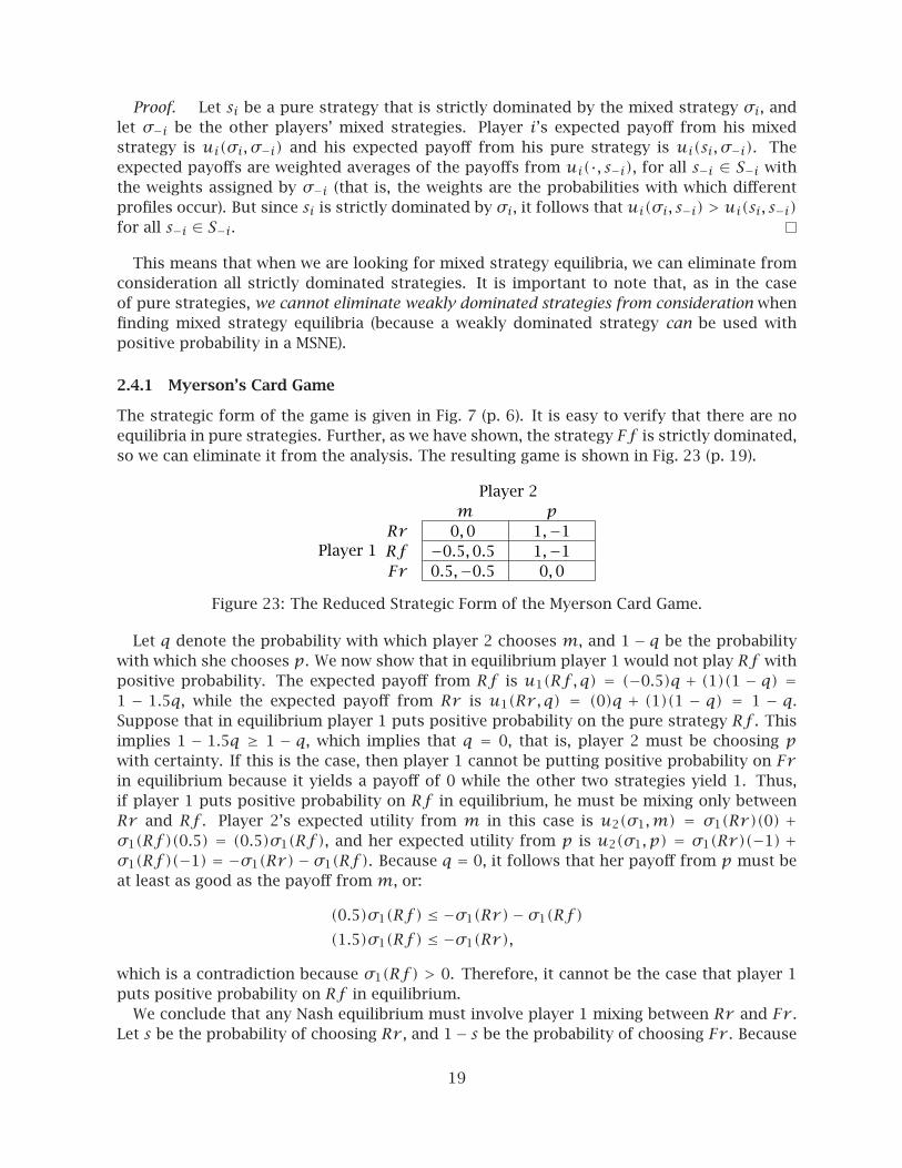
The strategic form of the game is given in Fig. 7 (p. 6). It is easy to verify that there are noequilibria in pure strategies. Further, as we have shown, the strategy Ff is strictly dominated,so we can eliminate it from the analysis. The resulting game is shown in Fig. 23 (p. 19).

Player 1

Player 2m p

Rr 0,0 1,−1Rf −0.5,0.5 1,−1Fr 0.5,−0.5 0,0

Figure 23: The Reduced Strategic Form of the Myerson Card Game.

Let q denote the probability with which player 2 chooses m, and 1 − q be the probabilitywith which she chooses p. We now show that in equilibrium player 1 would not play Rf withpositive probability. The expected payoff from Rf is u1(Rf , q) = (−0.5)q + (1)(1 − q) =1 − 1.5q, while the expected payoff from Rr is u1(Rr , q) = (0)q + (1)(1 − q) = 1 − q.Suppose that in equilibrium player 1 puts positive probability on the pure strategy Rf . Thisimplies 1 − 1.5q ≥ 1 − q, which implies that q = 0, that is, player 2 must be choosing pwith certainty. If this is the case, then player 1 cannot be putting positive probability on Frin equilibrium because it yields a payoff of 0 while the other two strategies yield 1. Thus,if player 1 puts positive probability on Rf in equilibrium, he must be mixing only betweenRr and Rf . Player 2’s expected utility from m in this case is u2(σ1,m) = σ1(Rr)(0) +σ1(Rf)(0.5) = (0.5)σ1(Rf), and her expected utility from p is u2(σ1, p) = σ1(Rr)(−1) +σ1(Rf)(−1) = −σ1(Rr)− σ1(Rf). Because q = 0, it follows that her payoff from p must beat least as good as the payoff from m, or:

(0.5)σ1(Rf) ≤ −σ1(Rr)− σ1(Rf)(1.5)σ1(Rf) ≤ −σ1(Rr),

which is a contradiction because σ1(Rf) > 0. Therefore, it cannot be the case that player 1puts positive probability on Rf in equilibrium.

We conclude that any Nash equilibrium must involve player 1 mixing between Rr and Fr .Let s be the probability of choosing Rr , and 1− s be the probability of choosing Fr . Because

19

player 1 is willing to mix, the expected payoffs from the two pure strategies must be equal.Thus, (0)q+ (1)(1−q) = (0.5)q+ (0)(1−q), which implies that q = 2/3. Since player 2 mustbe willing to randomize as well, her expected payoffs from the pure strategies must also beequal. Thus, (0)s+(−0.5)(1−s) = (−1)s+(0)(1−s), which implies that s = 1/3. We concludethat the unique mixed strategy Nash equilibrium of the card game is

⟨(1/3[Rr], 2/3[Fr]) ,

(2/3[m], 1/3[p]

)⟩.

That is, player 1 raises for sure if he has a red (winning) card, and raises with probability1/3 if he has a black (losing) card. Player 2 meets with probability 2/3 when she sees player 1raise in equilibrium. The expected utility payoff in this unique equilibrium for player 1 is:

(0.5) [2/3(2)+ 1/3(1)]+ (0.5) [1/3 (2/3(−2)+ 1/3(1))+ 2/3(−1)] = 1/3,

and the expected payoff for player 2, computed analogously, is −1/3. If you are risk-neutral,you should only agree to take player 2’s role if offered a pre-play bribe of at least $0.34because you expect to lose $0.33.

2.4.2 Another Simple Game

To illustrate the algorithm for solving strategic form games, we now go through a detailedexample using the game from Myerson, p. 101, reproduced in Fig. 24 (p. 20). The algorithmfor finding all Nash equilibria involves (a) checking for solutions in pure strategies, and (b)checking for solutions in mixed strategies. Step (b) is usually the more complicated one,especially when there are many pure strategies to consider. You will need to make variousguesses, use insights from dominance arguments, and utilize the remarks about optimalmixed strategies here.

Player 1

Player 2L M R

U 7,2 2,7 3,6D 2,7 7,2 4,5

Figure 24: A Strategic Form Game.

We begin by looking for pure-strategy equilibria. U is only a best response to L, but thebest response to U is M . There is no pure-strategy equilibrium involving player 1 choosingU . On the other hand, D is a best response to both M and R. However, only L is a bestresponse to D. Therefore, there is no pure-strategy equilibrium with player 1 choosing Dfor sure. This means that any equilibrium must involve a mixed strategy for player 1 withsupp(σ1) = {U,D}.

Turning now to player 2’s strategy, we note that there can be no equilibrium with player2 choosing a pure strategy either. This is because player 1 has a unique best response toeach of her three strategies, but we have just seen that player 1 must be randomizing inequilibrium.

We now have to make various guesses about the support of player 2’s strategy. We knowthat it must include at least two of her pure strategies, and perhaps all three. There are fourpossibilities to try.

20

• supp(σ2) = {L,M,R}. Since player 2 is willing to mix, she must be indifferent betweenher pure strategies, and therefore:

2σ1(U)+ 7σ1(D) = 7σ1(U)+ 2σ1(D) = 6σ1(U)+ 5σ1(D).

We require that the mixture is a valid probability distribution, or σ1(U)+ σ1(D) = 1.

Note now that 2σ1(U)+ 7σ1(D) = 7σ1(U)+ 2σ1(D)⇒ σ1(U) = σ1(D) = 0.5. However,7σ1(U) + 2σ1(D) = 6σ1(U) + 5σ1(D) ⇒ σ1(U) = 3σ1(D), a contradiction. Therefore,there can be no equilibrium that includes all three of player 2’s strategies in the supportof her mixed strategy.

• supp(σ2) = {M,R}. Since player 1 is willing to mix, it must be the case that 2σ2(M) +3σ2(R) = 7σ2(M)+4σ2(R)⇒ 0 = 5σ2(M)+σ2(R), which is clearly impossible becauseboth σ2(M) > 0 and σ2(R) > 0. Hence, there can be no equilibrium where player 2’ssupport consists of M and R.

• supp(σ2) = {L,M}. Because player 1 is willing to mix, it follows that 7σ2(L)+2σ2(M) =2σ2(L)+ 7σ2(M)⇒ σ2(L) = σ2(M) = 0.5. Further, because player 2 is willing to mix, itfollows that 2σ1(U)+ 7σ1(D) = 7σ1(U)+ 2σ1(D)⇒ σ1(U) = σ1(D) = 0.5.

So far so good. We now check for profitable deviations. If player 1 is choosing eachstrategy with positive probability, then choosing R would yield player 2 an expectedpayoff of (0.5)(6) + (0.5)(5) = 5.5. Thus must be worse than any of the strategies inthe support of her mixed strategy, so let’s check M . Her expected payoff from M is(0.5)(7) + (0.5)(2) = 5. That is, the strategy to which she assigns positive probabilityyields an expected payoff strictly higher than any of the strategies in the support of hermixed strategy. Therefore, this cannot be an equilibrium either.

• supp(σ2) = {L,R}. Since player 1 is willing to mix, it follows that 7σ2(L) + 3σ2(R) =2σ2(L) + 4σ2(R) ⇒ 5σ2(L) = σ2(R), which in turn implies σ2(L) = 1/6, and σ2(R) =5/6. Further, since player 2 is willing to mix, it follows that 2σ1(U)+7σ1(D) = 6σ1(U)+5σ1(D)⇒ σ1(D) = 2σ1(U), which in turn implies σ1(U) = 1/3, and σ1(D) = 2/3.

Can player 2 do better by choosing M? Her expected payoff would be (1/3)(7) +(2/3)(2) = 11/3. Any of the pure strategies in the support of her mixed strategyyields an expected payoff of (1/3)(2) + (2/3)(7) = (1/3)(6) + (2/3)(5) = 16/3, whichis strictly better. Therefore, the mixed strategy profile:

⟨(σ1(U) = 1/3, σ1(D) = 2/3) , (σ2(L) = 1/6, σ2(R) = 5/6)

⟩

is the unique Nash equilibrium of this game. The expected equilibrium payoffs are 11/3for player 1 and 16/3 for player 2.

This exhaustive search for equilibria may become impractical when the games becomelarger (either more players or more strategies per player). There are programs, like the lateRichard McKelvey’s Gambit, that can search for solutions to many games.

2.4.3 Choosing Numbers

Players 1 and 2 each choose a positive integer up to K. Thus, the strategy spaces are both{1,2, . . . , K}. If the players choose the same number then player 2 pays $1 to player 1,

21

otherwise no payment is made. Each player’s preferences are represented by his expectedmonetary payoff. The claim3 is that the game has a mixed strategy Nash equilibrium inwhich each player chooses each positive integer with equal probability.

It is easy to see that this game has no equilibrium in pure strategies: If the strategy profilespecifies the same numbers, then player 2 can profitably deviate to any other number; ifthe strategy profile specifies different numbers, then player 1 can profitably deviate to thenumber that player 2 is naming. However, this is a finite game, and so Nash’s Theorem tellsus there must be an equilibrium. Thus, we know we should be looking for one in mixedstrategies.

The problem here is that there is an infinite number of potential mixtures we have toconsider. We attack this problem methodically by looking at types of mixtures instead ofindividual ones. One focal mixture is where each number is chosen with the same probability.Since there are K numbers, this probability is 1/K.

We now apply Proposition 1. Since all strategies are in the support of this mixed strategy,it is sufficient to show that each strategy of each player results in the same expected payoff.(That is, we only use the first part of the proposition.) Player 1’s expected payoff from eachpure strategy is 1/K(1)+ (1− 1/K) (0) = 1/K because player 2 chooses the same number withprobability 1/K and a different number with the complementary probability. Similarly, player2’s expected payoff is 1/K(−1) + (1− 1/K) (0) = −1/K. Thus, this strategy profile is a mixedstrategy Nash equilibrium.

Is this the only MSNE? Let (σ∗1 , σ∗2 ) be a MSNE where σ∗i (k) is the probability that player

i’s mixed strategy assigns to the integer k. Given that player 2 uses σ∗2 , player 1’s expectedpayoff to choosing the number k is σ∗2 (k). From Proposition 1, if σ∗1 (k) > 0, then σ∗2 (k) ≥σ∗2 (j) for all numbers j. That is, if player 1 assigns positive probability to choosing somenumber k, then the equilibrium probability with which player 2 is choosing this numbermust be at least as great as the probability of any other number. If this were not the case,it would mean that there exists some number m ≠ k which player 2 chooses with a higherprobability in equilibrium. But in that case, player 1’s equilibrium strategy would be strictlydominated by the strategy that chooses m with a higher probability (because it would yieldplayer 1 a higher expected payoff). Therefore, the mixed strategy σ∗1 could not be optimal, acontradiction.

Since σ∗2 (j) > 0 for at least some j, it follows that σ∗2 (k) > 0. That is, because player2 must choose some number, she must assign a strictly positive probability to at least onenumber from the set. But because the equilibrium probability of choosing k must be at leastas high as the probability of any other number, the probability of k must be strictly positive.

We conclude that in equilibrium, if player 1 assigns positive probability to some arbitrarynumber k, then player 2 must do so as well.

Now, player 2’s expected payoff if she chooses k is −σ∗1 (k), and since σ∗2 (k) > 0, it mustbe the case that σ∗1 (k) ≤ σ∗1 (j) for all j. This follows from Proposition 1. To see this,note that if this did not hold, it would mean that player 1 is choosing some number mwith a strictly lower probability in equilibrium. However, in this case player 2 could dostrictly better by switching to a strategy that picks m because the expected payoff wouldimprove (the numbers are less likely to match). But this contradicts the optimality of player2’s equilibrium strategy σ∗2 .

3It is not clear how you get to this claim. This is the part of game theory that often requires some inspiredguesswork and is usually the hardest part. Once you have an idea about an equilibrium, you can check whetherthe profile is one. There is usually no mechanical way of finding an equilibrium.

22

What is the largest equilibrium probability with which k is chosen by player 1? We knowthat it cannot exceed the probability assigned to any other number. Because there are Knumbers, this means that it cannot exceed 1/K. To see this, note that if there was somenumber to which the assigned probability was strictly greater than 1/K, then there must besome other number with a probability strictly smaller than 1/K, and then σ∗1 (k) would haveto be no greater than that smaller probability. We conclude that σ∗1 (k) ≤ 1/K.

We have now shown that if in equilibrium player 1 assigns positive probability to somearbitrary number k, it follows that this probability cannot exceed 1/K. Hence, the equilibriumprobability of choosing any number to which player 1 assigns positive probability cannotexceed 1/K.

But this now implies that player 1 must assign 1/K to each number and mix over all availablenumbers. Suppose not, which would mean that player 1 is mixing over n < K numbers. Fromthe proof above, we know that he cannot assign more than 1/K probability to each of thesen numbers. But because his strategy must be a valid probability distribution, the individualprobabilities must sum up to 1. In this case, the sum up to n/K < 1 because n < K. The onlyway to meet the requirement would be to assign at least one of the numbers a strictly largerprobability, a contradiction. Therefore, σ∗1 (k) = 1/K for all k.

A symmetric argument establishes the result for player 2. We conclude that there are noother mixed strategy Nash equilibria in this game.

2.4.4 Defending Territory

General A is defending territory accessible by 2 mountain passes against General B. GeneralA has 3 divisions at his disposal and B has 2. Each must allocate divisions between the twopasses. A wins the pass if he allocates at least as many divisions to it as B does. A successfullydefends his territory if he wins at both passes.

General A has four strategies at his disposal, depending on the number of divisions heallocates to each pass: SA = {(3,0), (2,1), (1,2), (0,3)}. General B has three strategies he canuse: SB = {(2,0), (1,1), (0,2)}. We construct the payoff matrix as shown in Fig. 25 (p. 23).

General A

General B(2,0) (1,1) (0,2)

(3,0) 1,−1 −1,1 −1,1(2,1) 1,−1 1,−1 −1,1(1,2) −1,1 1,−1 1,−1(0,3) −1,1 −1,1 1,−1

Figure 25: Defending Territory.

This is a strictly competitive game, which (not surprisingly) has no pure strategy Nashequilibrium. Thus, we shall be looking for MSNE. Denote a mixed strategy of General A by(p1, p2, p3, p4), and a mixed strategy of General B by (q1, q2, q3).

First, suppose that in equilibrium q2 > 0. Since General A’s expected payoff from hisstrategies (3,0) and (0,3) are both less than any of the other two strategies, it follows thatin such an equilibrium p1 = p4 = 0. In this case, General B’s expected payoff to his strategy(1,1) is then −1. However, either one of the other two available strategies would yield ahigher expected payoff. Therefore, q2 > 0 cannot occur in equilibrium.

23

Given that in any equilibrium q2 = 0, what probabilities would B assign to the other twostrategies in equilibrium? Since q2 = 0, it follows that q3 = 1 − q1. General A’s expectedpayoff to (3,0) and (2,1) is 2q1 − 1, and the payoff to (1,2) and (0,3) is 1− 2q1. If q1 < 1/2,then in any equilibrium p1 = p2 = 0. In this case, B has a unique best response, whichis (2,0), which implies that in equilibrium q1 = 1. But if this is the case, then either ofA’s strategies (3,0) or (2,1) yields a higher payoff than any of the other two, contradictingp1 = p2 = 0. Thus, q < 1/2 cannot occur in equilibrium. Similarly, q1 > 1/2 cannot occur inequilibrium. This leaves q1 = q3 = 1/2 to consider.

If q1 = q3 = 1/2, then General A’s expected payoffs to all his strategies are equal. Wenow have to check whether General B’s payoffs from this profile meet the requirements ofProposition 1. That is, we have to check whether the payoffs from (2,0) and (0,2) are thesame, and whether this payoff is at least as good as the one to (1,1). The first condition is:

−p1 − p2 + p3 + p4 = p1 + p2 − p3 − p4

p1 + p2 = p3 + p4 = 1/2

General B’s expected payoff to (2,0) and (0,2) is then 0, so the first condition is met. Notenow that since p1 +p2 +p3 +p4 = 1, we have 1− (p1 +p4) = p2 +p3. The second conditionis:

p1 − p2 − p3 + p4 ≤ 0

p1 + p4 ≤ p2 + p3

p1 + p4 ≤ 1− (p1 + p4)p1 + p4 ≤ 1/2

Thus, we conclude that the set of mixed strategy Nash equilibria in this game is the set ofstrategy profiles:

((p1, 1/2− p1, 1/2− p4, p4

),(

1/2,0, 1/2))

where p1 + p4 ≤ 1/2.

2.4.5 Choosing Two-Thirds of the Average

(Osborne, 34.1) Each of 3 players announces an integer from 1 to K. If the three integers aredifferent, the one whose integer is closest to 2/3 of the average of the three wins $1. If two ormore integers are the same, $1 is split equally between the people whose integers are closestto 2/3 of the average.

Formally, N = {1,2,3}, Si = {1,2, . . . , K}, and �S = S1 × S2 × S3. There are K3 differentstrategy profiles to examine, so instead we analyze types of profiles.

Suppose all three players announce the same number k ≥ 2. Then 2/3 of the average is 2/3k,and each gets $1/3. Suppose now one of the players deviates to k− 1. Now 2/3 of the averageis 2/3k − 2/9. We now wish to show that the player with k − 1 is closer to the new 2/3 of theaverage than the two whose integers where k:

2/3k− 2/9− (k− 1) < k− (2/3k− 2/9)k > 5/6

Since k ≥ 2, the inequality is always true. Therefore, the player with k− 1 is closer, and thushe can get the entire $1. We conclude that for any k ≥ 2, the profile (k, k, k) cannot be a Nashequilibrium.

24

The strategy profile (1,1,1), on the other hand, is NE. (Note that the above inequality worksjust fine for k = 1. However, since we cannot choose 0 as the integer, it is not possible toundercut the other two players with a smaller number.)

We now consider an strategy profile where not all three integers are the same. First con-sider a profile, in which one player names a highest integer. Denote an arbitrary such profileby (k∗, k1, k2), where k∗ is the highest integer and k1 ≥ k2. Two thirds of the averagefor this profile is a = 2/9(k∗ + k1 + k2). If k1 > a, then k∗ is further from a than k1,and therefore k∗ does not win anything. If k1 < a, then the difference between k∗ and a isk∗−a = 7/9k∗− 2/9k1− 2/9k2. The difference between k1 and a is a−k1 = 2/9k∗− 7/9k1+ 2/9k2.The difference between the two is then 5/9k∗+ 5/9k1− 4/9k2 > 0, and so k1 is closer to a. Thusk∗ does not win and the player who offers it is better off by deviating to k1 and sharing theprize. Thus, no profile in which one player names a highest integer can be Nash equilibrium.

Consider now a profile in which two players name highest integers. Denote this profile by(k∗, k∗, k) with k∗ > k. Then a = 4/9k∗ + 2/9k. The midpoint of the difference between k∗and k is 1/2(k∗ + k) > a. Therefore, k is closer to a and wins the entire $1. Either of the twoother players can deviate by switching to k and thus share the prize. Thus, no such profilecan be Nash equilibrium.

This exhausts all possible strategy profiles. We conclude that this game has a unique Nashequilibrium, in which all three players announce the integer 1.

2.4.6 Voting for Candidates

(Osborne, 34.2) There are n voters, of which k support candidate A and m = n − k supportcandidate B. Each voter can either vote for his preferred candidate or abstain. Each voter getsa payoff of 2 if his preferred candidate wins, 1 if the candidates tie, and 0 if his candidateloses. If the citizen votes, he pays a cost c ∈ (0,1).

(a) What is the game with m = k = 1?

(b) Find the pure-strategy Nash equilibria for k =m.

(c) Find the pure-strategy Nash equilibria for k < m.

We tackle each part in turn:

(a) Let’s draw the bi-matrix for the two voters who can either (V)ote or (A)bstain. This isdepicted in Fig. 26 (p. 25).

A Supporter

B SupporterV A

V 1− c,1− c 2− c,0A 0,2− c 1,1

Figure 26: The Election Game with Two Voters.

Since 0 < c < 1, this game is exactly like the Prisoners’ Dilemma: both citizens vote andthe candidates tie.

(b) Here, we need to consider several cases. (Keep in mind that each candidate has an equalnumber of supporters.) Let nA ≤ k denote the number of citizens who vote for A and

25

let nB ≤ m denote the number of citizens who vote for B. We restrict our attention tothe case where nA ≥ nB (the other case is symmetric, so there is no need to analyzeit separately). We now have to consider several different outcomes with correspondingclasses of strategy profiles: (1) the candidates tie with either (a) all k citizens voting forA or (b) some of them abstaining; (2) some candidate wins either (a) by one vote or (b)by two or more votes. Thus, we have four cases to consider:

(a) nA = nB = k: Any voting supporter who deviates by abstaining causes his can-didate to lose the election and receives a payoff of 0 < 1 − c. Thus, no votingsupporter wants to deviate. This profile is a Nash equilibrium.

(b) nA = nB < k: Any abstaining supporter who deviates by voting causes his candi-date to win the election and receives a payoff of 2 − c > 1. Thus, an abstainingsupporter wants to deviate. This profile is not Nash equilibrium.

(c) nA = nB +1 or nB = nA+1: Any abstaining supporter of the losing candidate whodeviates by voting causes his candidate to tie and increases his payoff from 0 to1− c. These profiles are not Nash equilibria.

(d) nA ≥ nB+2 or nB ≥ nA+2: Any supporter of the winning candidate who switchesfrom voting to abstaining can increase his payoff from 2 − c to 2. Thus, theseprofiles cannot be Nash equilibria.

Therefore, this game has a unique Nash equilibrium, in which everybody votes and thecandidates tie.

(c) Let’s apply very similar logic to this part as well:

(a) nA = nB ≤ k: Any supporter of B who switches from abstaining to voting causesB to win and improves his payoff from 1 to 2− c. Such a profile cannot be a Nashequilibrium.

(b) nA = nB + 1 and nB = nA + 1, with nA < k: Any supporter of the losing candidatecan switch from abstaining to voting and cause his candidate to tie, increasing hispayoff from 0 to 1− c. Such a profile cannot be a Nash equilibrium.

(c) nA = k and nB = k + 1: Any supporter of A can switch from voting to abstainingand save the cost of voting for a losing candidate, improving his payoff from −cto 0. Such a profile cannot be a Nash equilibrium.

(d) nA ≥ nB + 2 or nB ≥ nA + 2: Any supporter of the winning candidate can switchfrom voting to abstaining and improve his payoff from 2 − c to 2. Such a profilecannot be a Nash equilibrium.

Thus, when k < m, the game has no Nash equilibrium (in pure strategies).

3 Symmetric Games

A useful class of normal form games can be applied in the study of interactions which in-volve anonymous players. Since the analyst cannot distinguish between the player, it followsthat they have the same strategy sets (otherwise the analyst could tell them apart from thedifferent strategies they have available). These games are most often used for 2 player inter-actions.

26

Definition 10. A two-player normal form game is symmetric if the players’ sets of strate-gies are the same and their payoff functions are such that

u1(s1, s2) = u2(s2, s1) for every (s1, s2) ∈ S.

That is, player 1’s payoff from a profile in which he chooses strategy s1 and his opponentchooses s2 is the same as player 2’s payoff from a profile, in which he chooses s1 and player1 chooses s2. Note that these do not really have to be equal, it just has to be the case thatthe outcomes are ordered the same way for each player. (Thus, we’re not doing interpersonalcomparisons.) Once we have the same ordinal ranking, we can always rescale the appropriateutility function to give the same numbers as the other. Therefore, we continue using theequality but while keeping in mind that it does not have to hold. A generic example, as inFig. 27 (p. 27) might help. You can probably already see that Prisoners’ Dilemma and Stag

A BA w,w x,yB y,x z, z

Figure 27: The Symmetric Game.

Hunt are symmetric while BoS is not. We now define a special solution concept:

Definition 11. A strategy profile (s∗1 , s∗2 ) is a symmetric Nash equilibrium if it is a Nash

equilibrium and s∗1 = s∗2 .

Thus, in a symmetric Nash equilibrium, all players choose the same strategy in equilib-rium. For example, consider the game in Fig. 28 (p. 27). It has three Nash equilibria in purestrategies: (A,A), (C,A), and (A,C). Only (A,A) is symmetric.

A B CA 1,1 2,1 4,1B 1,2 5,5 3,6C 1,4 6,3 0,0

Figure 28: Another Symmetric Game.

Let’s analyze several games where looking for symmetric Nash equilibria make sense.

3.1 Heartless New Yorkers

A pedestrian is hit by a taxi (happens quite a bit in NYC). There are n people in the vicinityof the accident, and each of them has a cell phone. The injured pedestrian is unconsciousand requires immediate medical attention, which will be forthcoming if at least one of the npeople calls for help. Simultaneously and independently each of the n bystanders decideswhether to call for help or not. Each bystander obtains v units of utility if the injuredperson receives help. Those who call pay a personal cost of c < v . If no one calls, eachbystander receives a utility of 0. Find the symmetric Nash equilibrium of this game. What isthe probability no one calls for help in equilibrium?

We begin by noting that there is no symmetric Nash equilibrium in pure strategies: If nobystander calls for help, then one of them can do so and receive a strictly higher payoff of

27

v − c > 0. If all call for help, then any one can deviate by not calling and receive a strictlyhigher payoff v > v−c. (Note that there are n asymmetric Nash equilibria in pure strategies:the profiles, where exactly one bystander calls for help and none of the others does, are allNash equilibria. However, the point of the game is that these bystanders are anonymous anddo not know each other. Thus, it makes sense to look for a symmetric equilibrium.)

Thus, the symmetric equilibrium, if one exists, should be in mixed strategies. Let p bethe probability that a person does not call for help. Consider bystander i’s payoff of thismixed strategy profile. If each of the other n− 1 bystanders does not call for help, help willnot arrive with probability pn−1, which means that it will be called (by at least one of thesebystanders) with probability 1− pn−1.

What is i to do? His payoff is [pn−1(0) + (1 − pn−1)v] = (1 − pn−1)v if he does not call,and v − c if he does. From Proposition 1, we must find p such that the payoffs from his twopure strategies are the same:

(1− pn−1)v = v − cpn−1 = c/v

p∗ = (c/v)1n−1

Thus, when all other bystanders play p = p∗, i is indifferent between calling and not calling.This means he can choose any mixture of the two, and in particular, he can choose p∗ as well.Thus, the symmetric mixed strategy Nash equilibrium is the profile where each bystandercalls with probability 1− p∗.

To answer the second question, we compute the probability which equals:

p∗n = (c/v)

nn−1

Since n/(n− 1) is decreasing in n, and because c/v < 1, it follows that the probability thatnobody calls is increasing in n. The unfortunate (but rational) result is that as the number ofbystanders goes up, the probability that someone will call for help goes down.4 Intuitively,the reason for this is that while person i’s payoff to calling remains the same regardless ofthe number of bystanders, the payoff to not calling increases as that number goes up, sohe becomes less likely to call. This is not surprising. What is surprising, however, is thatas the size of the group increases, the probability that at least one person will call for helpdecreases.

3.2 Rock, Paper, Scissors

Two kids play this well-known game. On the count of three, each player simultaneouslyforms his hand into the shape of either a rock, a piece of paper, or a pair of scissors. If bothpick the same shape, the game ends in a tie. Otherwise, one player wins and the other losesaccording to the following rule: rock beats scissors, scissors beats paper, and paper beatsrock. Each obtains a payoff of 1 if he wins, −1 if he loses, and 0 if he ties. Find the Nashequilibria.

We start by the writing down the normal form of this game as shown in Fig. 29 (p. 29).

4There is an infamous case of this dynamic in action: the murder of Kitty Genovese in New York City in1964, with 38 neighbors looking on without calling the police.

28

Player 1

Player 2R P S

R 0,0 −1,1 1,−1P 1,−1 0,0 −1,1S −1,1 1,−1 0,0

Figure 29: Rock, Paper, Scissors.

It is immediately obvious that this game has no Nash equilibrium in pure strategies: Theplayer who loses or ties can always switch to another strategy and win. This game is sym-metric and we shall look for symmetric mixed strategy equilibria first.

Let p,q, and 1−p−q be the probability that a player chooses R, P , and S respectively. Wefirst argue that we must look only at completely mixed strategies (that is, mixed strategiesthat put positive probability on every available pure strategy). Suppose not, and so p1 = 0in some (possibly asymmetric) MSNE. If player 1 never chooses R, then playing P is strictlydominated by S for player 2, and so he will play either R or S. However, if player 2 neverchooses P , then S is strictly dominated by R for player 1, and so player 1 will choose either Ror P in equilibrium. However, since player 1 never chooses R, it follows that he must chooseP with probability 1. But in this case player 2’s optimal strategy will be to play S, to whicheither R or S are better choices than P . Therefore, p1 = 0 cannot occur in equilibrium. Similararguments establish that in any equilibrium, any strategy must be completely mixed.

We now look for a symmetric equilibrium. Player 1’s payoff from R is p(0)+ q(−1)+ (1−p−q)(1) = 1−p−2q. His payoff from P is 2p+q−1. His payoff from S is q−p. In a MSNE,the payoffs from all three pure strategies must be the same, and so

1− p − 2q = 2p + q − 1 = q − pSolving these equalities yields p = q = 1/3. Thus, whenever player 2 plays the three purestrategies with equal probability, player 1 is indifferent between his pure strategies, andso can play any mixture. In particular, he can play the same mixture as player 2, whichwould leave player 2 indifferent among his pure strategies. This verifies the first condition inProposition 1. Because these strategies are completely mixed, we are done. The symmetricNash equilibrium is (1/3, 1/3, 1/3).

Is this the only MSNE? We already know that any mixed strategy profile must consist onlyof completely mixed strategies in equilibrium. Arguing in a way similar to that for thepure strategies, we can show that there can be no equilibrium in which players put differ-ent weights on their pure strategies.

Generally, you should check for MSNE in all combinations. That is, you should checkwhether there are equilibria, in which one player chooses a pure strategy and the other mixes;equilibria, in which both mix; and equilibria in which neither mixes. Note that the mixturesneed not be over the entire strategy spaces, which means you should check every possiblesubset.

Thus, in a 2×2 two-player game, each player has three possible choices: two in pure strate-gies and one that mixes between them. This yields 9 total combinations to check. Similarly,in a 3 × 3 two-player game, each player has 7 choices: three pure strategies, one completelymixed, and three partially mixed. This means that we must examine 49 combinations! (Youcan see how this can quickly get out of hand.) Note that in this case, you must check bothconditions of Proposition 1.

29

4 Strictly Competitive Games

This is a special class of games that is not studied any more as much as it used to be.Nevertheless, it is important to know about them because (a) the results are not difficult, and(b) the results will be useful in later parts of the course.

A strictly competitive game is a two-player game where players have strictly opposed rank-ings over the outcomes. A good example is Matching Pennies. That is, when comparingvarious strategy profiles, whenever one player’s payoff increases, the other player’s payoffdecreases. Thus, there is no room for coordination or compromise. More formally,

Definition 12. A two-player strictly competitive game is a two-player game with the prop-erty that, for every two strategy profiles, s, s′ ∈ S,

u1(s) > u1(s′)� u2(s) < u2(s′).

A special case of strictly competitive games are the zero-sum games where the sum of thetwo players’ payoffs is zero (e.g. Matching Pennies).

Player 1

Player 2L R

U 3,2 0,4D 6,1 1,3

Figure 30: A Strictly Competitive Game.

Consider the (non-zero-sum) strictly competitive game in Fig. 30 (p. 30). What is the worst-case scenario that player 1 could ever face? This is the case where player 2 chooses R, whichyields a smaller payoff to player 1 whether he chooses U or D (he gets 0 < 3 if he chooses Uand 1 < 6 if he chooses D).

More generally, the worst payoff that player i can get when he plays the (possibly mixed)strategy σi is defined by

wi(σi) ≡ minsj∈Sj

ui(si, sj).

Which means that we look at all strategies available to player j to find the one that givesplayer i the smallest possible payoff if he plays σi. In other words, if player i chooses σi, heis guaranteed to receive a payoff of at least wi(σi). This is the smallest payoff that player 2can hold player 1 to given player 1’s strategy. A security strategy gives player i the best ofthe worst. That is, it solves maxσi∈Σi wi(σi):

Definition 13. A strategy σi ∈ Σi for player i is called a security strategy if it solves theexpression

maxσi∈Σi

minsj∈Sj

ui(σi, sj),

which also represents player i’s security payoff.

Returning to our example in Fig. 30 (p. 30), player 1’s security strategy is D because giventhat player 2 is minimizing player 1’s payoff by playing R, player 1 can maximize it by choos-ing D (because 1 > 0). Similarly, player 1 can hold player 2 to at most 3 by playing D, towhich player 2’s best response is R.

Although there is no general relationship between security strategies and equilibriumstrategies, an important exception exists for strictly competitive games.

30

Proposition 3. If a strictly competitive game has a Nash equilibrium, (σ∗1 , σ∗2 ), then σ∗1 is

a security strategy for player 1 and σ∗2 is a security strategy for player 2.

Note that in our example, the unique Nash equilibrium is (D,R), which consists of theexact security strategies we found for both players.

If we look at Matching Pennies, we note that w1(H) = −1 when s2 = T , and w1(T) = −1when s2 = H. On the other hand w1(1/2) = 0, and so player 1’s security strategy is to mixbetween his two actions with equal probability. A symmetric argument establishes the sameresult for the other player. Again, the unique Nash equilibrium of this game is in securitystrategies.

5 Five Interpretations of Mixed Strategies

See Osborne and Rubinstein’s A Course in Game Theory, pp. 37-44 for a more detailed treat-ment of this subject. Here, I only sketch several substantive justifications for mixed strate-gies.

5.1 Deliberate Randomization

The notion of mixed strategy might seem somewhat contrived and counter-intuitive. One(naıve) view is that playing a mixed strategy means that the player deliberately introducesrandomness into his behavior. That is, a player who uses a mixed strategy commits to arandomization device which yields the various pure strategies with the probabilities specifiedby the mixed strategy. After all players have committed in this way, their randomizationdevices are operated, which produces the strategy profile. Each player then consults hisrandomization device and implements the pure strategy that it tells him to. This producesthe outcome for the game.

This interpretation makes sense for games where players try to outguess each other (e.g.strictly competitive games, poker, and tax audits). However, it has two problems.

First, the notion of mixed strategy equilibrium does not capture the players’ motivationto introduce randomness into their behavior. This is usually done in order to influence thebehavior of other players. We shall rectify some of this once we start working with extensiveform games, in which players move can sequentially.

Second, and perhaps more troubling, in equilibrium a player is indifferent between hismixed strategy and any other mixture of the strategies in the support of his equilibriummixed strategies. His equilibrium mixed strategy is only one of many strategies that yield thesame expected payoff given the other players’ equilibrium behavior.

5.2 Equilibrium as a Steady State

Osborne (and others) introduce Nash equilibrium as a steady state in an environment inwhich players act repeatedly and ignore any strategic link that may exist between successiveinteractions. In this sense, a mixed strategy represents information that players have aboutpast interactions. For example, if 80% of past play by player 1 involved choosing strategy Aand 20% involved choosing strategy B, then these frequencies form the beliefs each playercan form about the future behavior of other players when they are in the role of player1. Thus, the corresponding belief will be that player 1 plays A with probability .8 and B

31

with probability .2. In equilibrium, the frequencies will remain constant over time, and eachplayer’s strategy is optimal given the steady state beliefs.

5.3 Pure Strategies in an Extended Game

Before a player selects an action, he may receive a private signal on which he can base hisaction. Most importantly, the player may not consciously link the signal with his action (e.g. aplayer may be in a particular mood which made him choose one strategy over another). Thissort of thing will appear random to the other players if they (a) perceive the factors affectingthe choice as irrelevant, or (b) find it too difficult or costly to determine the relationship.

The problem with this interpretation is that it is hard to accept the notion that playersdeliberately make choices depending on factors that do not affect the payoffs. However,since in a mixed strategy equilibrium a player is indifferent among his pure strategies in thesupport of the mixed strategy, it may make sense to pick one because of mood. (There areother criticisms of this interpretation, see O&R.)

5.4 Pure Strategies in a Perturbed Game

Harsanyi introduced another interpretation of mixed strategies, according to which a gameis a frequently occurring situation, in which players’ preferences are subject to small randomperturbations. Like in the previous section, random factors are introduced, but here they af-fect the payoffs. Each player observes his own preferences but not that of other players. Themixed strategy equilibrium is a summary of the frequencies with which the players choosetheir actions over time.

Establishing this result requires knowledge of Bayesian Games, which we shall obtain laterin the course. Harsanyi’s result is so elegant because even if no player makes any effort touse his pure strategies with the required probabilities, the random variations in the payofffunctions induce each player to choose the pure strategies with the right frequencies. Theequilibrium behavior of other players is such that a player who chooses the uniquely opti-mal pure strategy for each realization of his payoff function chooses his actions with thefrequencies required by his equilibrium mixed strategy.

5.5 Beliefs

Other authors prefer to interpret mixed strategies as beliefs. That is, the mixed strategyprofile is a profile of beliefs, in which each player’s mixed strategy is the common belief ofall other players about this player’s strategies. Here, each player chooses a single strategy,not a mixed one. An equilibrium is a steady state of beliefs, not actions. This interpretationis the one we used when we defined MSNE in terms of best responses. The problem here isthat each player chooses an action that is a best response to equilibrium beliefs. The set ofthese best responses includes every strategy in the support of the equilibrium mixed strategy(a problem similar to the one in the first interpretation).

6 The Fundamental Theorem (Nash, 1950)

Since this theorem is such a central result in game theory, we shall present a somewhatmore formal version of it, along with a sketch of the proof. A finite game is a game withfinite number of players and a finite strategy space. The following theorem due to John Nash

32

(1950) establishes a very useful result which guarantees that the Nash equilibrium conceptprovides a solution for every finite game.

Theorem 1. Every finite game has at least one mixed strategy equilibrium.

Recall that a pure strategy is a degenerate mixed strategy. This theorem does not assert theexistence of an equilibrium with non-degenerate mixing. In other words, every finite gamewill have at least one equilibrium, in pure or mixed strategies.

The proof requires the idea of best response correspondences we discussed. However, itis moderately technical in the sense that it requires the knowledge of continuity propertiesof correspondences and some set theory. I will give the outline of the proof here but youshould read Gibbons pp. 45-48 for some additional insight.

Proof. Recall that player i’s best response correspondence BRi(σ−i) maps each strategyprofile σ to a set of mixed strategies that maximize player i’s payoff when the other playersplay σ−i. Let ri = BRi(σ) for all σ ∈ Σ denote player i’s best reaction correspondence. Thatis, it is the set of best responses for all possible mixed strategy profiles. Define r : Σ ⇒ Σ tobe the Cartesian product of the ri. (That is, r is the set of all possible combinations of theplayers best responses.) A fixed point of r is a strategy profile σ∗ ∈ r(σ∗) such that, foreach player, σ∗i ∈ ri(σ∗). In other words, a fixed point of r is a Nash equilibrium.

The second step involves showing that r actually has a fixed point. Kakutani’s fixed pointtheorem establishes four conditions that together are sufficient for r to have a fixed point:

1. Σ is compact,5 convex,6 nonempty subset of a finite-dimensional Euclidean space;7

2. r(σ) is nonempty for all σ ;

3. r(σ) is convex for all σ ;

4. r is upper hemi-continuous.8

We must now show that Σ and r meet the requirements of Kakutani’s theorem. Since Σi is asimplex of dimension #Si − 1 (that is, the number of pure strategies player i has less 1), it iscompact, convex, and nonempty. Since the payoff functions are continuous and defined oncompact sets, they attain maxima, which means r(σ) is nonempty for all σ . To see the thirdcase, note that if σ ′ ∈ r(σ) and σ ′′ ∈ r(σ) are both best response profiles, then for eachplayer i and α ∈ (0,1),

ui(ασ ′i + (1−α)σ ′′i , σ−i) = αui(σ ′i , σ−i)+ (1−α)ui(σ ′′i , σ−i),

that is, if both σ ′i and σ ′′i are best responses for player i to σ−i, then so is their weightedaverage. Thus, the third condition is satisfied. The fourth condition requires sequences butthe intuition is that if it were violated, then at least one player will have a mixed strategy

5Any sequence in Σ has a subsequence that converges to a point in Σ. Alternatively, a compact set is closedand bounded.

6Σ is convex if every convex combination of any two points in the set is also in the set.7For our purposes, the Euclidean space is the same as Rn, i.e. the set of n-tuples of real numbers.8A correspondence is upper-hemicontinuous at x0 if every sequence in which r(x) → x0 has a limit which

lies in the image set of x0. That is, if (σn, σn) → (σ , σ ) with σn ∈ r(σn), then σ ∈ r(σ). This condition isalso sometimes referred to as r(·) having a closed graph.

33

that yields a payoff that is strictly better than the one in the best response correspondence,a contradiction.

Thus, all conditions of Kakutani’s fixed point theorem are satisfied, and the best reactioncorrespondence has a fixed point. Hence, every finite game has at least one Nash equilibrium.

Somewhat stronger results have been obtained for other types of games (e.g. games withuncountable number of actions). Generally, if the strategy spaces and payoff functions arewell-behaved (that is, strategy sets are nonempty compact subset of a metric space, andpayoff functions are continuous), then Nash equilibrium exists. Most often, some games maynot have a Nash equilibrium because the payoff functions are discontinuous (and so the bestreply correspondences may actually be empty).

Note that some of the games we have analyzed so far do not meet the requirements of theproof (e.g. games with continuous strategy spaces), yet they have Nash equilibria. This meansthat Nash’s Theorem provides sufficient, but not necessary, conditions for the existence ofequilibrium. There are many games that do not satisfy the conditions of the Theorem butthat have Nash equilibrium solutions.

Now that existence has been established, we want to be able to characterize the equilibriumset. Ideally, we want to have a unique solution, but as we shall see, this is a rare occurrencewhich happens only under very strong and special conditions. Most games we consider willhave more than one equilibrium. In addition, in many games the set of equilibria itself ishard to characterize.

34