Game Theory at Work - WUR
160
Game Theory at Work: OR models and algorithms to solve multi-actor heterogeneous decision problems
Transcript of Game Theory at Work - WUR

Game Theory at Work:OR models and algorithms to solve multi-actor
heterogeneous decision problems


Game Theory at Work:OR models and algorithms to solve multi-actor
heterogeneous decision problems
M. Elena Saiz
Proefschriftter verkrijging van de graad van doctor
op gezag van de rector magnificusvan Wageningen Universiteit,
Prof. dr. M.J. Kropff,in het openbaar te verdedigenop woensdag 24 oktober 2007
des namiddags te half twee in de Aula

Game Theory at Work: OR models and algorithms to solve multi-actor heterogeneousdecision problemsPhD thesis Wageningen Universiteit - with references - with summaries in English,Dutch and SpanishSaiz M. E., 2007ISBN: 978-90-8504-769-8

Promotor: Prof. ir. A.J.M. BeulensHoogleraar Toegepaste Informatiekunde
Prof. dr. ir. J.G.A.J. van der VorstHoogleraar Logistiek en Operationele Research
Co-promotor: Dr. E.M.T. HendrixUniversitair Hoofddocent bij de LeerstoelgroepOperationele Research en Logistiek
Samenstelling promotiecommissie:
Prof. dr. F. Plastria Vrije Universiteit BrusselProf. dr. J. Puerto Albandoz Universidad de SevillaProf. dr. A.M.A. van Deemen Radboud Universiteit NijmegenProf. dr. E.C. van Ierland Wageningen Universiteit
Dit onderzoek is uitgevoerd binnen de Mansholt Graduate School of Social Sciences.


Abstract
The objective of this thesis is to explore the potential of combining Game Theory (GT)models with Operations Research (OR) modelling. This includes development of algorithmsto solve these complex OR models for different empirical situations. The challenge is to getGT“at work”by applying such models and techniques to practical cases. Four different caseswith a challenge on the development of algorithms are studied.A first case illustrates a multiple coalition formation game in which membership rules anddifferent transfer schemes are described. Given the GT model and the OR model, the goalis to develop methods for checking stability of coalition structures. A new mathemati-cal programming formulation, crucial for the development of the algorithms, is elaborated.Available data is used to determine which stable coalitions appear and which procedures(transfer schemes) can be used to make coalitions stable. Also the influence of membershiprules (whether actors are free to become a member) is investigated. Main conclusion is thattransfer schemes are useful to be implemented to obtain stable coalitions. Moreover, differentmembership rules, e.g. veto or majority voting of current members, generate different resultswith and without transfer schemes.A second case studies a model of coalition formation in politics with n parties trying to forma government. Given the number of parties n and policy dimension m (number of items),computational algorithms are developed to compute all possible majority coalitions and pref-erences of parties over those coalitions. Application to Dutch data and theoretical examplesleads to testing of hypotheses with surprising results with respect to coalition formation suchas: being a first mover is not necessarily advantageous, being less flexible is not necessarilyadvantageous, forming a minimal winning coalition is not necessarily advantageous.A third case describes a two-stage location-quantity game where n > 2 firms are competingon m > 2 markets. The space where the firms can locate are nodes on a network. Analyticalsolutions for the supplying decisions and properties for determining the number of suppliersto each market are derived. In finding the equilibria, a complete enumeration algorithm anda local search algorithm are used. Two cases are elaborated to illustrate the procedures andthe analytical results.The last case deals with a competitive facility location problem in which the concept ofStackelberg leader-follower problem is applied. The follower problem and leader problem areglobal optimisation problems. Branch-and-Bound (B&B) algorithms that guarantee to findthe optimum of both problems are designed.Key words: Game theory, operations research, optimisation methods, algorithms.


Preface
By doing a PhD abroad, one is confronted with the culture etiquettes. As Spaniard, I triedto explain that we have sun but also snow; that we do not always take a “siesta” but a longlunch-break and keep working until 6, 7 or 8 p.m., we have central heating and we have thebeautiful letter “n”, without “her” what would happen with “manana”. . . ? We do not makeappointments with friends, we just simply call and meet later the same day or “manana”, wedo not have so many rules leading to “if-then”behaviour, we do not have a birthday calendarin the toilet, we just remember or forget the birthdays, but it is well accepted by friends.Yes, we are very good with jokes but we do not always speak so loud . . . only when we aremore than two.
Everything started in Sevilla. At the beginning of the summer of 2001 I moved to Sevillato start my PhD studies at the department of Statistics and Operations Research. There,the Professor of the group assigned Rafael Blanquero as my supervisor. Thanks to RafaI became enthousiastic about the PhD, and thanks to Rafa I came to Wageningen. Rafa,without you today would not have been possible.
I would like to thank my promoters Prof. ir. Adrie J.M. Beulens, Prof. dr. ir. JackG.A.J. van der Vorst and my daily supervisor and co-promotor Dr. Eligius M.T. Hendrix.Adrie and Jack, first of all thanks for all the support, assistance, encouragement, criticismand philosophical questions during our meetings. I have learnt a lot from them, as yousurely know. Adrie, thanks for all your active, positive, productive comments, and foralways having a smile for everything. Jack, what can I say, since you arrived to our groupeverything changed . . . to be better. Already in our first meeting I was impressed. At thatmoment I was already in my second year of PhD without any research question and anyproposal, just going on here and there. You are the responsible on getting funds for the finaltwo years of this adventure. You taught me lot of things during the meetings. For both,thanks for all the thinking on what is this thesis about, what are the research questions andfor all the input on my“researcher” education. Eligius, thank you for your patient, guidance,thanks for all the thinkings, ideas, support, encouragement, jokes, we spent many manyhours discussing the research. If I have to evaluate you as a supervisor, for me you are thebest. I will be back to you later, as family.
I would like now to thank to the whole team of Operationele Research en Logistiek: Frits,thanks for asking now and then how I am doing; Theo, now Real Madrid is doing betterwith the Dutch players ehh; Joke and Karin, the girls, it was always funny to have some girlsgossiping; Niels, we know how to respect and share the bad and good PhD mood, I hopeyou will have a successful career; the newcomer Jelena or Enna, she introduced a nice drinktradition on Fridays. And finally Ria, you were always so positive, kind, and a smile in themorning, thank you, I know that the bottles of wine were not the reason :-)
And during the last years I would also like to thank the team of Toegepaste Infor-

matekunde: Kees, Rob, Gert Jan, Ayalew, Dik, Mark, Yuan, Sebastiaan, Gerard, Jan, Kees,Sjoukje, Huub, Maarten and again . . . Ria. I also want to express my gratitude to Paul vanBeek for his helpful comments and interest in my research.
People from the Leeuwenborch: Ekko was responsible to bring me here to Wageningen.Then I met the whole STACO team. Thanks to all of you, you were always very supportiveand new ideas were on the table at all of the meetings. Thanks to Juan Carlos, the Mexicanpart of the team. Thanks to Rob, Hans-Peter and Michael, clever and wise people.
I would like to express my gratitude to Agnieszka and Annelies, I really enjoyed to worktogether with you, it was a pleasure. I wish you all the best in your new positions. Andmany thanks for introducing me to Ad. I want to express my gratitude to Jose Fernandezand Blas Pelegrın; research via e-mail is difficult but not impossible. Thanks for all theinput-output of our common research.
Thanks are also extended to colleagues from the Social Sciences Department: to Amberand Janneke, I have always enjoyed a lot our coffee breaks outside; to Lan Ge, for sharingpre-conference nervios and post-talk fun, and for the years in here; to Morteza, my squashpartner the first years. I would like to thank all people from Environmental Economics andNatural Resources Group and the Mansholt team. I should also mention the secretaries ofthe Leeuwenborch.
Specific gratitude goes to De Bongerd. I have all of the members in my heart. Thanksa lot for helping me to get rid of the stress or whatever I had in my head: Rob (2 Rob“os”),Henry, Rene, Wendy, John . . . but special words go to Ellen and Ingi. Ellen, thanks forall the very nice moments/talks doing step, indoor biking or whatever out of sports. Sorryfor missing a lot during my last PhD year . . . Ingi, thanks for being the one to start anongelofelijk-party-team with Ellen, you and me, thanks for the laughs together, the chats,the kinderen, the gezellige momentjes and thanks for being always there and for your support,enthusiasm and ideas about all the weird things I was doing. I must say thank to you foryou being as you are. To both and all the team of the Bonderd, thanks for making many ofmy stuff easier.
I must also say thanks to Joanna. Last years were very gezellig, I had a lot of fun andI would never forget your 2006 birthday party. I would like to express my gratitude to theRural corner of the Leeuwenborch. Jan Douwe, siempre has conseguido sacarme una sonrisa,gracias (todavıa me debes una cerveza). Special thanks goes to Kei and Gustavo for sharingPhD up and downs, gracias por todo vuestro apoyo. A big word of thanks goes to Petra. Ihad a great time with you talking in Spanutch (siempre curiosa sobre el significado/raız demuchas palabras), biking and discussing life issues. Ans and Cees, many thanks for takingcare of the PhD team. I will never forget you and your gezellig parties. Ans, thanks givingus advice on the layout of our books. I would like to thank all the good friends I have metduring my years in Wageningen, specially to Adolf, Olga, Toni, Marga, (Francesca)2, Axel,Andre, Ada y la ultima en llegar, Noa “Ribera del Duero”. I also wish to thank to Nelly forkeeping my neck connecting my head and back.
I would like to thank Costanza, when she was living in Wageningen everything wasdifferent. I am glad that we met and we had/have many talks and discussions about life,thanks for sharing that with me. “Jenny” Co, “Il Sasha piu adattato, zio felice, tranne nellapioggia. Un grande bacio e noi manchiamo a voi” :-O . Lola, Paul and Joek (het hondje),what can I say . . . I do not have enough pages to say how important you are in my life,not only in Wageningen. Thanks for all your support and for the many many many goodmoments we have had. Thanks for sharing your friendship, for cheering me up when I needed.It maybe helped the jamon and chorizo for Paultje :-). Out of jokes, I love you and you willbe always on my heart and my life. Special thanks goes to Lola. I had great time with you,thank you for your humor, your encourage, for sharing the good and the bad on our PhD

roken-punt-moments. And thanks for all the help. Gracias por todo, “Jenny” galleguina,eres muy grande.
I would like to thank all my friends in Spain: Laurita, Clara “caminera”, Elvis, Jelen“gemela”, Corita, Marta “logrono”, Marta “mingo”, Ana, Marıa, Fran, Avel y Marta,Valen,Yolanda, Almu y Sara, Mercedes y Elenita, Esperanza y Lina. Thank you for all the supportand emails. Os quiero muchısimo, gracias por todo vuestro apoyo, por mantenerme al dıade vuestras cositas. Un besazo enorme.
Gracias Eligius. I do not know how to express all my gratitude to you; thank you forbeing you, for taking me at your place when I came to Wageningen, for all the support, forall the mathematics and algorithmic ideas, for all the encouragement, for all the fun and thevery nice talks while sharing the wine from Spain, for all the personal chats we had, for all theunderstanding, for all the gezellig during the travels to Spain by car, in summary, THANKS.As I always said, thanks for being my family, my father and . . .mother in Wageningen. Youare great.
Finally I would like to thank to my family. Gracias Mama y Papa, Papa y Mama, graciasa mis hermanitos (Javier-Javi y Antonio-Tono). Gracias a todos, sin vosotros habrıa sidoimposible hacer esto. Ha sido muy duro estar lejos de vosotros, pero ha merecido la pena, yasabeis, personalmente. Miles, millones, no existe el numero para decir GRACIAS por todovuestro apoyo en mis objetivos, por todas vuestras visitas, por vuestras llamadas telefonicas,POR ESTAR AHI. Gracias al resto de mi familia, pero tambien tengo que decir gracias a miqueridita tıa y a mi prima favorita, gracias por todo vuestro apoyo, yes, lo he sentido muydentro de mi corazon. Y a Sasha, mi perrito, gracias por compartir conmigo los ultimos anosen Wageningen. Esta tesis va dirigida a todos vosotros . . . pero tengo que hacer una mencionespecial a alguien que estoy segura vais a respetar.
Esta tesis va dirigida especialmente a ti, abuelita, te conozco perfectamente y se quehabrıas sido la primera en coger un avion y estar aquı conmigo hoy, disfrutando como nuncade esta parafernalia, hablando spanglish, aunque no tuvieras ni idea de ingles, tu sabes,hablando espanol bien alto, claro y, por supuesto, despacio . . . que estos guiris no se enterande otra forma ehh!? Y ademas habrıas sido la reina de la fiesta, como siempre. Un beso alcielo desde la loca Tierra. Tu nieta.
(English translation: this thesis is specially dedicated to my grandma, I know you per-fectly and I know that you would have been the first, taking a plane and being in here withme, enjoying as never this paraphernalia, talking Spanglish by you know, talking Spanishtoo loud, clear and, of course, slow . . . these guiris do not understand in another way ehh!?Furthermore, you would have been the queen of the party, as always. One big kiss to thesky from the crazy Earth. Your granddaughter.)


CONTENTS
1 General Introduction 1
1.1 Introduction . . . . . . . . . . . . . . . . . . . . . . . . . . . . . . . . . . . . 1
1.2 Game Theory Introduction . . . . . . . . . . . . . . . . . . . . . . . . . . . . 4
1.3 Operations Research . . . . . . . . . . . . . . . . . . . . . . . . . . . . . . . . 6
1.4 Research Objective and Questions . . . . . . . . . . . . . . . . . . . . . . . . 10
1.5 Research Approach and Outline of the Thesis . . . . . . . . . . . . . . . . . . 12
2 On the Computation of Stability in Multiple Coalition Formation Games 17
2.1 Introduction . . . . . . . . . . . . . . . . . . . . . . . . . . . . . . . . . . . . 18
2.2 Game Theoretic Background: Definitions and Concepts . . . . . . . . . . . . 19
2.3 Mathematical Programming Notation and Stability Check . . . . . . . . . . 22
2.4 Description of the Algorithm . . . . . . . . . . . . . . . . . . . . . . . . . . . 28
2.5 Illustration of the Algorithm . . . . . . . . . . . . . . . . . . . . . . . . . . . 30
2.6 Conclusions . . . . . . . . . . . . . . . . . . . . . . . . . . . . . . . . . . . . . 36
3 On Computing Negotiation Positions and Preferences in a Spatial CoalitionModel 37
3.1 Introduction . . . . . . . . . . . . . . . . . . . . . . . . . . . . . . . . . . . . 38
3.2 Algorithms for the Different Procedures . . . . . . . . . . . . . . . . . . . . . 44
3.3 Hypothesis Testing . . . . . . . . . . . . . . . . . . . . . . . . . . . . . . . . 50
3.4 Conclusions . . . . . . . . . . . . . . . . . . . . . . . . . . . . . . . . . . . . . 58
4 Methods for Computing Nash Equilibria of a Location-Quantity Game 61
4.1 Introduction . . . . . . . . . . . . . . . . . . . . . . . . . . . . . . . . . . . . 62
4.2 Location-Quantity Game: Problem Formulation . . . . . . . . . . . . . . . . 63
4.3 Methods for Computing Nash Quantities and Nash Locations . . . . . . . . . 72
4.4 Numerical Illustration . . . . . . . . . . . . . . . . . . . . . . . . . . . . . . . 76
4.5 Conclusions . . . . . . . . . . . . . . . . . . . . . . . . . . . . . . . . . . . . . 82
5 On a Branch-and-Bound Approach for a Huff-like Stackelberg Location Problem 85
5.1 Introduction . . . . . . . . . . . . . . . . . . . . . . . . . . . . . . . . . . . . 86
5.2 Description of the Problem . . . . . . . . . . . . . . . . . . . . . . . . . . . . 87
5.3 A Branch-and-Bound Algorithm for the Medianoid (follower) Problem . . . . 89
i

ii Contents
5.4 A Branch-and-Bound Algorithm for the Leader Problem . . . . . . . . . . . 95
5.5 Numerical Examples . . . . . . . . . . . . . . . . . . . . . . . . . . . . . . . . 97
5.6 Conclusions and Future Work . . . . . . . . . . . . . . . . . . . . . . . . . . 104
6 General Discussion and Conclusions 107
6.1 Introduction . . . . . . . . . . . . . . . . . . . . . . . . . . . . . . . . . . . . 107
6.2 Brief Outline of the Research . . . . . . . . . . . . . . . . . . . . . . . . . . . 107
6.3 Main Conclusions and Research Questions . . . . . . . . . . . . . . . . . . . 108
6.4 Discussion of the Research . . . . . . . . . . . . . . . . . . . . . . . . . . . . 112
Bibliography 117
Summary 123
Samenvatting 127
Resumen 133
List of Publications 139
Curriculum Vitae 141

CHAPTER 1
General Introduction
1.1 Introduction
“The work of managers, of scientists, of engineers, of lawyers – the work that steers the
course of society and its economic and governmental organizations – is largely work
of making decisions and solving problems. It is work of choosing issues that require
attention, setting goals, finding or designing suitable courses of action, and evaluating
and choosing among alternative actions. The first three of these activities – fixing
agendas, setting goals, and designing actions – are usually called problem solving;
the last, evaluating and choosing, is usually called decision making. Nothing is more
important for the well-being of society than that this work be performed effectively,
that we address successfully the many problems requiring attention at the national level
(the budget and trade deficits, AIDS, national security, the mitigation of earthquake
damage), at the level of business organizations (product improvement, efficiency of
production, choice of investments), and at the level of our individual lives (choosing a
career or a school, buying a house).”
(Simon et al. (1986), p.19 )
Decision making is present in daily life. Governments, organizations, workers are confrontedeveryday with different decision problems and with the need to address and resolve theseproblems. The moment we wake up everyday we start making decisions and try to dothings the best way or as good as possible given the decision making situation. Often onetries to maximise a kind of utility in order to reach an objective. Some decisions can bemade automatically, that is, the decision maker has been confronted with a similar problemmany times and has learned to arrive at a solution using a predefined algorithm (solutionmethod). These are called programmed decisions. Other decisions can be characterised asnon-programmed and less structured, also called unstructured decisions. That means thatthe decision maker has to cope with unusual and less structured situations in which decisionsare made based on information or intuition. Decision making takes place when a need fora decision is recognized. Based on it a problem is delineated and solution alternatives aregenerated. The alternatives are evaluated based on the objective to generate a ranking onpreference order of alternatives. Based on the evaluation and identification of expected risks,consequences and values of each alternative, one can select the best-favourable alternativerelated to the objective of the decision maker.
Keen and Scott-Morton (1978) identified five different approaches of decision making:

2 Game Theory at Work
• A Rational way of decision making, in which the manager is completely informed,knows all the alternatives and can make an optimal choice (’objective rational-ity’);
• A satisfycing way of decision making, in which a decision alternative is soughtthat satisfies all participants (’bounded rationality’);
• A organisational procedures way of decision making, which sees decisions as theoutput of standard operating procedures invoked by organisational subunits;
• A political way of decision making, in which a decision is seen as a result ofnegotiations between actors; power and influence determine the outcome of anygiven decision;
• A individual differences way of decision making, which presupposes a very im-portant role for the character of the individual, and in which personality andstyle are of great importance.
In van der Vorst (2000) the satisfycing approach is emphasised as the most relevant:
“The rational way of decision making could be used for the reordering of standard
products; and the political way of decision making could be used when selecting another
supplier. But in general, a mix of the mentioned approaches is applied when making
a decision (Benders et al. (1983)). According to Simon (1976) ’most human decision
making, whether individual or organisational, is concerned with the discovery and
selection of satisfactory alternatives; only in exceptional cases is it concerned with the
discovery and selection of optimal alternatives’. Because of this bounded rationality
the choice in most decision making situations is for satisfycing decisions.”
(van der Vorst (2000), p.58)
In many decision situations the decision problem can be decomposed into components thatare to be dealt with in parallel and/or subsequently. In other words, decision makers face thedecision problem in a simultaneous or in a step-by-step way. Decision situations may alsoinvolve more than one decision maker, which leads to a competing or cooperating situation.For example, when a supermarket has to decide about where to locate and other competingsupermarkets already exist or plan to locate at the same area. Or if a political party does nothave a majority in the government, negotiations with other parties can take place in order toform a majority government. Decisions have in common that all are made in order to solveproblems. Unfortunately, not all problems are easily solved without modelling approachesand the development of associated solvers (computational algorithms).
We focus on decision making problems following the rational way of decision. Withinthe context of decision making processes, it is well accepted (Simon (1976), Keen and Scott-Morton (1978) and van der Vorst (2000)) to use Model Based Decision Support Systems(MBDSS) with associated solvers for models incorporated. These models are then meantto help to generate decision alternatives and/or to evaluate consequences of decision alter-natives. In this thesis we focus on a special class of optimisation models and algorithms(solvers) that can play an important role in such MBDSS. Models are made to representthe decision situation under study. Solvers are developed that allow the modeller to obtainefficiently and effectively optimal solutions for models developed. These “optimal” solutionscan be of great value in practical decision situations. In the remainder of this thesis, we usethe term “optimal” in the sense just described.
We hypothesise that Game Theory may have modelling merits to contribute to decisionmaking situations where decision makers have competing or cooperating objectives, underthe assumption that the decision makers are rational and they act in their best own interest.Game Theory is a key element for studying decision making problems involving two or moredecision makers. It provides concepts and applies mathematical models for selecting an opti-mal strategy considering the strategy of the others. In daily life, one can observe cooperation

General Introduction 3
in the form of club membership, alliances between companies and countries (sky alliance,NATO, EU) on all levels. Part of the cooperation incentives is economic; the signatories ofa coalition consider membership a win-win situation over non membership. Such incentivesdrive horizontal and vertical cooperation in supply chains and club formation between organ-isations and countries. One can also observe competitive situations, for example when twoor more chains are trying to get more market share from a common area and they competeon prices. Competition not only takes place in business, also games like tennis or chess arecompetitive.
Many real world decision problems need more elaboration than just optimizing only onevariable (e.g. time) or only one decision maker objective. Not only the number of decisionmakers plays a role, many problems involve decisions at many levels, over several periods oron a planning horizon. The objective is to guarantee to have an optimum. One could tryto handle it with a hierarchical approach, solving each subproblem at each level, in somecases, using the information obtained from the decisions made in earlier subproblems. Whenmore than one decision maker is involved, Game Theory gives us modelling techniques todo so. Game theory models are often applied to situations with few or symmetric multipledecision makers, which limits its modelling power. It is well accepted in literature that itis impossible to completely represent the real world in models. The real world and decisionsituations are too complex. Therefore, we aim at Game Theory models that are able tobetter represent or are able to represent more important features of an types of relationshipsof the real world. So we are trying to minimise the gap between our modelling requirementsand models actually built. In addition, we aim to develop solvers for these enhanced GameTheory models.
Results and models in Game Theory can be found in literature. These results are oftendue to basic models with two actors leading to analytical solutions or alternatively to moreactors that are all assumed to be the same; symmetric players. In this thesis we extend thesemodels by studying cooperative or competitive decision situations in the observable world:building new models in Game Theory and reformulating into Operations Research modelsto study cases with more than two heterogeneous actors. In this case, one has to applyand develop new Operations Research techniques, that is, modelling optimisation problemsand developing algorithms to solve them. Therefore, in order to compute the solutions it isrequired first to build new or to use existing Game Theory models for multi-actor coopera-tion; second to develop and reformulate these models using Operations Research techniques;and third to develop new algorithms for solving the models using sets of equalities, linearoptimisation, nonlinear optimisation, combinatorial optimisation, etc. If we look at relevantliterature and especially also at case descriptions in different areas such as environmentaldecisions, supply chain management decisions and political games, we find decision supportrequirements and decision situations that may benefit from a modelling approach using GameTheory models because of their modelling capabilities (e.g. to represent competing decisionmakers). As a consequence, it is of scientific and practical importance to research the valueof Game Theory models and associated solvers.
The objective of this thesis is to explore the potential of combining Game Theory mod-els with mathematical modelling and solve these complex Operations Research models bydeveloping algorithms in different empirical situations. The idea is to contribute filling thegap between theory and practice developing Operations Research models and algorithms forGame Theory models describing Decision Making problems. The challenge is to get GameTheory “at work” by applying such models and techniques to practical cases. This providesinsight into which concepts of Game Theory are practically applicable for which type ofcases, and on the other hand, get insight in the use of mathematical programming modelsand algorithms to reach the target.

4 Game Theory at Work
We first give a small overview on relevant Game Theory (GT) concepts and models inSection 1.2 and Operations Research (OR) techniques in Section 1.3. Section 1.4 specifiesthe objective of this thesis and the research questions. Section 1.5 elaborates the objective ofthe study and how the questions are investigated together with a brief outline of the thesis.
1.2 Game Theory IntroductionIn von Neumann and Morgenstern (1944) a clear introduction to what constitutes a game isgiven:
“First, one must distinguish between the abstract concept of a game, and the individualplays of that game. The game is simply the totality of the rules which describe it. Everyparticular instance at which the game is played – in a particular way – from beginningto end, is a play.
Second, the corresponding distinction should be made for the moves, which are thecomponent elements of the game. A move is the occasion of a choice between variousalternatives, to be made either by one of the players, or by some device subject tochance, under conditions precisely prescribed by the rules of the game. The move isnothing but this abstract ’occasion’, with the attendant details of description, – i.e. acomponent of the game. The specific alternative chosen in a concrete instance – i.e. ina concrete play – is the choice. Thus the moves are related to the choices in the sameway as the game is to the play. The game consists of a sequence of moves, and the playof a sequence of choices.
Finally, the rules of the game should not be confused with the strategies of the players.
Exact definitions will be given consequently, but the distinction which we stress must
be clear from the start. Each player selects his strategy – i.e. the general principles
governing his choices – freely. While any particular strategy may be good or bad –
provided that these concepts can be interpreted in an exact sense (...) – it is within the
player’s discretion to use or to reject it. The rules of the game, however, are absolute
commands. If they are ever infringed, then the whole transaction by definition ceases
to be the game described by those rules. In many cases it is even physically impossible
to violate them.”
(von Neumann and Morgenstern (1944), p. 49)
In this section, GT is briefly introduced and related to the focus of this thesis. For a moreprofound elaboration, interested readers are referred to other more specific texts on GT suchas Myerson (1991) or Shubik (1984). GT Models are games, which are basically definedby: number of players, set of available strategies, outcomes and payoffs associated with theoutcomes. GT concepts define the characteristics of the games. GT concepts give the detailsof the elements of the game (e.g. player, strategy, utility), details about the informationavailable to the players (e.g. complete, perfect), or how players choose their strategies (e.g.simultaneous) and other characteristics of the game like communication rules. Next, theseand some others GT concepts are introduced.
A game can be defined as a mathematical representation of a conflict situation. Theoutcome depends on mutual interaction between two or more rational individuals, calledplayers. A player can be defined as a decision maker in a decision problem: a person, agroup, an animal, or whatever entity. Depending on the number of players, games can beclassified as a two-person game, three-person game, and in general a N-person game, N > 2.
Games have rules specifying the actions the player can take, the information the playerhas available and the consequences of the decisions. Consequences usually are not only forthe player itself but also for the other players, which leads to a cooperative or to a competitive

General Introduction 5
situation. For example, in a tennis game, the objective is not only to hit the ball back to theother player but to hit it back in a way the other player cannot return it, which also dependson where the opponent is placed. A game must also include payoffs or utilities (profits of theplayers), i.e., the reward one gets. Set of alternatives is used to describe the different actionsor strategies among which a given player can choose on the feasible space of the game, asquoted from von Neumann and Morgenstern (1944), a move is the occasion of a choice, thespecific alternative chosen is the choice. A strategy defines a set of moves (choices) a playerwill follow in a game. The strategy set is the set of strategies all players have chosen.
There is a distinction between games with complete and games with incomplete informa-tion depending on the information the players have about the parameters of the game. Ingames with complete information, players have full information about the strategies and util-ity functions of the other players. In incomplete information games, players may or may notknow some information (strategies, payoffs or preferences) about the other players. Gamescan also be divided into games with perfect and imperfect information depending on theinformation the players have about the past behaviour. In games with perfect information,players have full information about the actions that have already taken place.
According to how players choose their strategies, there is a distinction between simultaneous-move games and sequential-move games. In simultaneous games, players choose their strate-gies simultaneously, in ignorance of the strategies of the others. Players must predict whatthe opponents will do. A game can also be defined as a simultaneous game when decisionsare not taken at the same moment but moves are in ignorance of what the rest of playersare doing. In sequential games, players make decisions in sequential order.
Based on the gains or losses by the players, there are zero-sum games and non-zero sumgames. The most common situation is to apply these games for two players. Zero-sum gamesare conflict/competitive situations; the gain of a player (set of players) is the loss of the otherplayer (set of players), i.e. the total benefits for the players, for every combination of theavailable strategies, sum to zero. In non-zero sum games, aggregate payoffs are differentfrom zero. Furthermore, non-zero sum games are not strictly competitive games.
Depending on the communication rules, distinction is made between non-cooperative andcooperative games. In non-cooperative games, players are unable to make enforceable agree-ments outside of those specified by the game. Any cooperation must be self-enforcing. Incooperative games, players can make enforceable agreements and form clubs before choosingtheir actions. Competition is between clubs and not between individuals.
Another distinction is between symmetric games or asymmetric games. In a symmetricgame, independently of the player who is playing a particular strategy, a player earns thesame payoff when she chooses the same strategy/action against her competitors. Otherwise,a game is called asymmetric. In games, players can be homogeneous or heterogeneous. Theoutcomes for heterogeneous players are not the same if they play the same strategy.
According to the rules of coalition negotiation, two different games can be outlined de-pending on whether or not the players are allowed to make utility side payments as anincentive for the members. If side-payments are allowed, a game is called Transferable Util-ity Game, otherwise it is called Non-Transferable Utility Game.
Another concept is that of externalities, positive or negative. A game with externali-ties occurs when a decision made by a player causes an effect in terms of benefits (positiveexternalities) or costs (negative externalities) to third parties (other players). Examplesare pollution (negative externalities) or public goods (positive externalities). Positive ex-ternalities are related to the free-rider problem. A free-rider gets the benefits from positiveexternalities but does not contribute to its costs.
In this thesis we use two main solution concepts in GT. One is the Nash equilibrium.Nash (1951) introduced the concept in which no player can be better off by following another

6 Game Theory at Work
strategy while the others remain unchanged. A Nash equilibrium is a set of strategies forthe players such that no player has an incentive to unilaterally deviate from her strategy. Atequilibrium, each player is using the strategy that is the best reply to the strategies chosenby the other players.
Definition 1. Nash Equilibrium: A Nash equilibrium is a profile of strategy choices such
that every strategy of the players is a best reply to the strategies chosen by the other players.
In a Nash equilibrium, no player has any incentive to deviate unilaterally from it.
The definition of Nash equilibrium using the concept of best responses is as follows:
Definition 2. The strategy profile (s∗1, . . . , s∗i , . . . , s∗n) ∈ S is a Nash equilibrium if for each
i ∈ N :
s∗i ∈ arg maxsi∈Si
(πi(s∗1, . . . , si, . . . , s
∗n))
where Si denotes the set of all possible strategies for player i and πi the utility function.
We also consider the classical concept of stability of coalitions introduced for cartel coali-tion formation (one coalition) by d’Aspremont et al. (1983), which is in fact close to theNash equilibrium concept. A coalition is stable if, on the one hand, for a member of thecoalition there is no incentive to free-ride (internal stability) and on the other hand, for anon-member there is no incentive to take part of the coalition (external stability).
Two GT models are relevant in this study. The first is due to the French economistAugustin Cournot, the Cournot competition model (Cournot (1838)). It originally describesa competitive model between firms producing a homogeneous product. Firms compete si-multaneously on quantities, choosing how much to deliver to markets. The objective of eachfirm is to maximise profit. The game belongs to the class of imperfect information. Thesecond relevant model was proposed by the German economist Heinrich Freiherr von Stack-elberg, the Stackelberg competition model (Stackelberg (1934)). It models behaviour of twocompeting players called the leader-follower. The leader player moves first and chooses astrategy, then the follower moves sequentially, knowing the decisions taken by the leader.This game belongs to the class of perfect information games.
In this thesis, we use most of the concepts outlined above in four different cases. In twoof the cases, more than one decision needs to be made, that is, decisions are made in a so-called two-level decision game. At each stage or level of decision, all the players make theirdecisions simultaneously. In these cases, we use the GT concept subgame perfect equilibrium,which means that at every stage/step a Nash equilibrium is computed.
In Section 1.5.1, an outline of the relevant concepts we use through this thesis is given.
1.3 Operations ResearchMost of the decisions that we make in daily life have a goal: optimising a set of variables,where variables mean characteristics defining a problem. Operations Research has beendefined in many books and articles. In Hillier and Lieberman (1986) a complete descriptionof what OR is given.

General Introduction 7
“Operations Research is concerned with optimal decision making in, and modelling of,deterministic and probabilistic systems that originate from real life. These applications,which occur in government, business, engineering, economics, and the natural andsocial sciences, are largely characterized by the need to allocate limited resources. Inthese situations, considerable insight can be obtained from scientific analysis such asthat provided by operations research. The contribution from the operations researchapproach stems primarily from:
1. Structuring the real life situation into a mathematical model, abstracting the es-sential elements so that a solution relevant to the decision maker’s objectives can besought. This involves looking at the problem in the context of the entire system.2. Exploring the structure of such solutions and developing systematic procedures forobtaining them.3. Developing a solution, including the mathematical theory, if necessary, that yields anoptimal value of the system measure of desirability (or possibly comparing alternativecourses of action by evaluating their measure).”
(Hillier and Lieberman (1986), p. 6)
Thus, first step in modelling using OR is the formulation of the objective and specification ofthe decision variables of the problem. Based on the objective and decision variables identified,a model can be constructed as a mathematical representation of the problem. Conditions onthe decision variables, like relationships between variables and bounds, define what it is calledconstraints of the problem. Constraints are defined by using mathematical equations and/orinequalities. All the points satisfying the constraints define what it is called the feasible area.The objective function is defined from the objective of the problem. The idea is to optimisethe objective function, maximising or minimising, subject to the constraints (if they exist).The objective function together with the constraints define the mathematical programmingmodel, also known as optimisation problem. The next step is to solve the model finding anoptimal solution. A solution for the optimisation problem satisfies the constraints (so-calleda feasible solution) and gives a numerical value to each of the decision variables. An optimalsolution is feasible and represents the most desirable value for the objective of the problem.It can happen that a problem has no optimal solution, only one or an infinite number. Mostof the cases, in order to solve an optimisation problem an algorithm is required. OR models(or optimisation models) and optimisation algorithms are described next.
1.3.1 Operations Research Models
In the process of decision making situations, mathematical techniques can be used. Asintroduced before, decision variables may be restricted by conditions like bounds or relationswith other variables, this is called a constrained optimisation problem. When there are noconstraints the problem is called unconstrained optimisation problem. Thus, a first basic wayon modelling a decision problem is considering the restrictions on the decision variables. Forexample, in the tennis game the feasible area where one is allowed to play has limits.
When a problem has been defined as constrained or unconstrained, more characteristicscan be used in modelling it. The decision variables of the problem may be continuous ordiscrete. In a linear programming problem (LP), the objective and the constraints are linearfunctions and the decision variables are continuous. When at least one of the constraints orthe objective function are non-linear, the problem is called a nonlinear optimisation problem(NLP). Within nonlinear optimisation problems, one can distinguish between smooth (whenderivatives exists for all the functions in the model) and non-smooth (not all the functionshave derivatives defined at all the points). More distinctions are: unconstrained NLP opti-misation, a NLP problem without constraints; quadratic programming in which the objective

8 Game Theory at Work
function have quadratic terms and the constraints are linear equalities and inequalities; con-vex programming, where the objective function is convex and constraints form a convex set;separable programming implies that the objective and the constraints are separable functions(a function where each term involves just a single variable, so that the function is separableinto a sum of functions of individual variables. (Hillier and Lieberman (1986)); non-convexprogramming refers to nonlinear programming problems not satisfying the assumptions ofconvex programming; or fractional programming dealing with the optimisation of an ob-jective function having the form of a fraction (or ratio). In general, several local minima(maxima if it is a maximisation problem) may exist. Global Optimisation aims at finding asolution which is guaranteed to be the global optimum within a predefined accuracy.
If decisions are hierarchically structured, the problem can be modelled by multi-leveloptimisation programming, which are hierarchical optimisation problems. If the number oflevels is two, the problem is called a Bilevel optimisation problem. In bilevel optimisationproblems, the mathematical programming problem contains an optimisation problem in theconstraints. Bilevel optimisation problems are close to the Stackelberg problem from GameTheory (Colson et al. (2005)).
Now consider that the decision variables are discrete, that is, variables are restricted tovalues specified by a discrete set. If all the variables are required to take integer values,then the problem is modelled by Integer Programming (IP). If in addition the objective andconstraints are linear the problem belongs to the class of Integer Linear Programming (ILP)problems. When the problem has integer variables and continuous variables, the problemis called a Mixed Integer Optimization Problem (MIP). A problem involving combinatorialchoices is called a Combinatorial Optimisation Problem.
Linear or non-linear, continuous or discrete, decision making problems may also involvea time horizon space. When decisions need to be made over several periods, the problem ismodelled by a multi-period problem. Otherwise, the problem is called a static programmingproblem. In Section 1.5.1 an outline of OR models relevant for the research in this thesis isgiven.
1.3.2 Operations Research Algorithms
An algorithm is a step-by-step procedure for solving a problem. It is usual that an algorithmrepeats several steps over and over again until the desired result is obtained. In that sense,algorithms are iterative processes. Consider a group of friends. A member knows a gossipbut she wants to keep it as exactly as possible, not running and inflating from mouth tomouth. Algorithm 1.1 shows a possible algorithm to solve the problem.
Algorithm 1.1 : Gossiping1Funct Gossiping1(set of friends,gossip)
1. List := set of friends2. while List is not empty3. x := Take a friend from List4. Tell the gossip5. Get the promise to not say anything6. Delete x from List7. OUTPUT: Desired objective

General Introduction 9
When writing algorithms, two questions arise: do the procedures reach the desired solutionand at what computational cost? As defined in Hendrix (2007), efficiency is the effort thealgorithm needs to be successful. Several efficiency indicators appear in literature. Usualindicators are the number of function evaluations and memory requirements necessary toreach the optimum. Another question is related to effectiveness: does the algorithm findwhat we want? Algorithm 1.1 is effective (assuming that they will keep the promise) but isit efficient? Algorithm 1.2 shows another possibility for solving the problem.
Algorithm 1.2 : Gossiping2Funct Gossiping2(set of friends,gossip)
1. Make an appointment with the set of friends2. Tell the gossip3. Get the promise to not say anything4. List := set of friends - set of friends showed up5. while List is not empty6. x := Take a friend from List7. Tell the gossip8. Get the promise to not say anything9. Delete x from List
10. OUTPUT: Desired objective
It can be seen that Algorithm 1.2 is not only effective but it is more efficient thanAlgorithm 1.1. In general, algorithms have an initialization step setting up the parametersto start iterations, iterative step performing the operations, and optimality test or stoppingrule checking if the current solution is the optimal. Now the focus will be on algorithmssolving the OR models outlined in Section 1.3.1.
The simplex algorithm (Dantzig (1963)) became a popular method for solving LP prob-lems. There are variants of the simplex algorithms like the upper bound technique, the dualsimplex method or parametric programming. Karmarkar (1984) introduced an interior pointmethod for solving LPs. This algorithm is a polynomial time algorithm which is superior (intheory) to exponential time algorithms, like the simplex method.
Dynamic Programming is a tool that allows solving problems by using recursive calls tosubproblems with the same structure and smaller size. Dynamic Programming models canbe formulated when decisions have to be made in a sequence and are interrelated. Each stageinfluences the decision at the next stage. A recursive relation exists identifying the optimalsolution of stage n given the optimal solution for stage (n+1). Thus, the solution procedureconsists of solving first the last stage and then recursively going backwards.
Combinatorial Optimisation Problems, Integer Programming (IP) and Integer LinearProgramming (ILP) problems are not easy to solve. In many cases there exists an expo-nential explosion on the size of the problem increasing the computational difficulty. Dealingwith these problems by enumeration can be computationally very expensive depending onthe number of variables and structure of the problem. A possible algorithm for solving ILPproblems uses LP methods by doing what is called LP-relaxation. However, this methoddoes not always find the optimal solution (Schrijver (1998)). New algorithms are necessary.An often used technique for solving ILP problems is the Branch-and-Bound method. Incontrast with a total enumeration method, the Branch-and-Bound approach uses a partialenumeration. Branch-and-Bound is also used to solve most of the Combinatorial Optimisa-tion problems. An alternative to Branch-and-Bound methods are the Cutting Plane methods(Gomory (1958)). There also exists many heuristic algorithms for solving combinatorial op-

10 Game Theory at Work
timisation problems where solutions may be not optimal but satisfactory.
In contrast with LP problems, for NLP Problems no single based-algorithm exists thatwill solve the problem. Sometimes one can derive explicit solutions based on analysis of firstorder optimality conditions. Traditionally this is called analytically solving. Algorithms havebeen developed to solve individual problems like the ones described in the former section.For these models, many different Search Algorithms have been developed during the lastdecades, procedures like Golden Section search, Penalty Approach, Steepest Ascent (descentif minimising) or Global Optimisation Methods. Branch-and-Bound methods are also usedto solve GO models. For solving convex nonlinear models, available methods are for example,interior point methods or ellipsoid methods. One of the procedures applied in this thesis isbased on Sequential Quadratic Programming (SQP) (Boggs and Tolle (1996)).
Multilevel programming optimisation problems can be solved by LP, ILP, Combinatorial,Dynamic or NLP techniques depending on the characteristics of the model. In Section 1.5.1,the methods used in this thesis are outlined.
1.4 Research Objective and QuestionsGT not only gives analytical results (theorems) but can also be applied to numerical casesto derive tendencies for multi-actor cooperation in different circumstances. The challengein this thesis is to build GT models based on GT concepts to describe economic incentivesfor multi-actor heterogeneous situations. First of all, one has to translate GT models intoMathematical Programming models. After that, for solving these models, algorithms haveto be developed using OR techniques. Therefore, the focus of the study is on supportingthe process of building models to represent decision situations and developing techniques tosolve these models. Summarising and being more explicit, Figure 1.1 shows the conceptualmodel of the thesis research.
Information from the decision problem is used to select which GT concepts are necessaryand applicable. From the GT concepts and the decision problem, one can build a GT model.Based on the GT model and from the objective(s) defined within the decision problem, amathematical programming model (optimisation model) is formalised. One should try tocode the problem in an appropriate way. With the mathematical definition of the model,algorithms are developed and used to interact with the decision problem. Interaction ofalgorithms and problem definition is made by testing and validating results according to theobjectives. The challenge is to build GT and OR models and the development of algorithmsfor solving decision situations with multiple, heterogeneous and asymmetric actors.
With this conceptual model, the research objective is specified: to develop or con-tribute to the development of usable GT models and OR methods to solve them in practicalsituations. In other words, assess the capability of GT to describe economic incentives forcomplex decision problems involving multiple actors. In order to do this, there is a need todevelop optimisation models and algorithms to implement analytical concepts and modelsfrom Cooperative/Non-Cooperative Game Theory and Competitive models such that theyare applicable to numerical cases in economic literature.
With respect to the scientific relevance, it is necessary to distinguish between its method-ological and theoretical gains. First of all, as explained above, the thesis aims to develop aset of methodological tools which allows us to do numerical analyses. Moreover, the thesisaims to construct a conceptual model that combines GT, OR and Social Sciences. This isof interest for all scientists involved in the field of research and, of course, specifically thoseinvolved in the study of GT models and OR techniques. The research aims to provide a

General Introduction 11
OptimisationModel
(OR Models)
OptimisationModel
(OR Models)
OptimisationModel
(OR Models)
GT ConceptsGT ConceptsGT Concepts
Algorithms (OR Methods)
Algorithms(OR Methods) Algorithms
(OR Methods)
GT ModelsGT ModelsGT Models
Decision P
roblem D
omain
Decision P
roblem D
omain
Decision P
roblem D
omain
Figure 1.1. Conceptual Model of Thesis Research.
useful contribution to at least the following areas of related concern:
• Building optimisation (OR) models based on GT concepts/models
• Developing OR techniques as tools to solve optimisation (OR) models based on GTconcepts/models with multiple heterogeneous actors
• Cases of cooperation and competition are used to show the applicability of the GTmodels and the OR techniques
We hypothesise that GT concepts and models might provide us with a valuable contribu-tion for supporting decision makers provided that we can make OR models and algorithmsto solve these models. We can translate these aims and hypothesis in the following researchquestions:
1. How do we formulate GT models for decision making situations with multiple hetero-geneous actors using GT concepts? How can we contribute to that modelling?
2. If we have GT based models: What appropriate coding can be used to translate aspecific GT model into a mathematical programming optimisation problem such thatit can be solved?
3. Which solution methods can be developed to solve these models?
4. How do the outcomes aid to analyse the decision makers problem? or What is thecontribution of the new outcomes to the decision makers problem?
The following describes how we deal with these questions.

12 Game Theory at Work
1.5 Research Approach and Outline of the ThesisGovernments (countries), Companies, Markets (oligopoly, duopoly, bilateral monopoly, andso on) lend themselves to game-theoretic analyses because the fate of each participant de-pends on the actions taken by the other participant or participants. Methods are developedto deal with finite strategy approaches (enumeration) and continuous decision problems basedon GT concepts.
1.5.1 Research Design: Selection of CasesThe conceptual model explained above connects GT concepts and models with OR modelsand algorithms. In illustrating the conceptual model, we use case study research. We areinterested in cases covering some or all of the following characteristics:
1. Empirical studies involving cooperation and/or competition between the different play-ers (actors)
2. Empirical studies in which more than two players are heterogeneous and asymmetric
3. Transferable Utility games and/or Non-Transferable Utility games
4. Multi-level decision problems. That is, best solutions are found by making severaldecisions at different stages, optimizing each of the sub-problems
5. Games with externalities (positive or negative), free-rider problems
6. Considering the possibility of different rules of coalition formation
7. Using concepts as Nash equilibria and stability analysis of coalitions
8. Different procedures on coalition formation
The starting points for each of the cases are from sources based on literature review.To illustrate cooperative/non-cooperative GT concepts/models we looked for models with achallenge on algorithmic development. In particular, for Chapter 2, we take the model fromEyckmans and Finus (2003a) where multiple coalition formation is considered. In the paperof Eyckmans and Finus (2003a), a case with six players was studied by doing calculation moreor less by hand. However, larger games require to develop algorithms to solve it. In Chapter3, we use the model from de Ridder and Rusinowska (2005) to apply two different proceduresof coalition formation and to test several hypotheses. The model is multidimensional andwith more than two heterogeneous players resulting into a computational challenge whenusing real data. One can illustrate the model in few dimensions and few players as was donein de Ridder and Rusinowska (2005). In order to apply the model to real data, it is necessaryto develop OR methods.
To illustrate competition models, we looked for cases involving competition on locationand competition on location and quantity (see e.g. Drezner and Hamacher (2004) and Nickeland Puerto (2005) for an overview on location theory). Chapter 4 is based on the model ofSarkar et al. (1997), a competitive game based on location-quantity decisions. They considersymmetric and fixed-entry at the markets, that is, all the firms (players) will enter the market.When considering asymmetric players and free-entry at the markets, algorithms for gettingequilibria at quantities and locations are needed. Finally, Chapter 5 is based on the work ofDrezner and Drezner (1998) with a follower and leader competing on facility location. Theproblem is a global optimisation problem and it has been solved for the follower problem inliterature. However, as far as we know, the leader-follower problem has not been addressedwith global optimisation methods giving a guarantee on finding the global optimum for the

General Introduction 13
leader. In summary, the objective is to contribute to these models extending the researcheither on the GT models and reformulation to OR models or the OR methods.
Solution methods are developed in order to find the most favourable solution to theobjective defined by the players. OR involves the construction of mathematical models.Models are a collection of mathematical relationships representing aspects of the situationunder study. We use concepts from GT to build models of the decision situation and applytechniques of OR to generate algorithms to obtain the optimal solution(s). Figure 1.2 rep-resents how the conceptual model is combined with the case studies applied in this thesis.
Figure 1.2. Conceptual model and case studies
From the conceptual model of the thesis research in Figure 1.1 and the characteristics of theresearch showed on Figure 1.2, an overview of the applied cases is shown in Tables 1.1, 1.2and 1.3.
1.5.2 Outline of the Thesis
Chapter 2 describes and studies a multiple coalition formation game. Particular attentionis paid to the analysis of the stability of coalitions under different membership rules. Theidea is to analyse stability of multiple agreements based on the classical stability conceptdeveloped for cartel stability (see d’Aspremont et al. (1983)). Cartel stability restricts coali-tion formation to only one agreement. When multiple coalition formation is considered, thestability concept is more complex: for a signatory there should be no incentives to leave itscoalition to join another one. Consequences of membership rules are modelled and studied.
Chapter 3 focuses on a model described in de Ridder and Rusinowska (2005) of multidi-mensional coalition formation in politics. In the model, a government consists of a majoritycoalition and a policy supported by this coalition. There are n parties trying to form a gov-ernment. A formed government has a policy agreement represented in a m-multidimensionalEuclidean policy space R
m. The complexity increases with the number of parties n and

14 Game Theory at Work
Table 1.1. GT concepts used in this thesis
Chapter 2 Chapter 3 Chapter 4 Chapter 5Complete information X X X XIncomplete informationPerfect information X XImperfect information X XSimultaneous moves X X XSequential moves X XZero sum XNon-zero sum X X XCooperative X XNon-cooperative X X X XAsymmetric players X X X XSymmetric playersHeterogeneous players X X X XHomogeneous playersTransferable Utility XNon-transferable Utility X X XExternalities XNon externalities X X XTwo-level decision making X XStackelberg XCournot X
Table 1.2. OR models used in this thesis
Chapter 2 Chapter 3 Chapter 4 Chapter 5UnconstrainedConstrained X X X XContinuous X X X XDiscrete X X XNLP X X X XCombinatorial Optimisation X XStatic X X X XDynamicConvex Optimization X X XGO XBilevel X
Table 1.3. OR algorithms used in this thesis
Chapter 2 Chapter 3 Chapter 4 Chapter 5Enumeration Algorithms X XBranch-and-Bound XAnalytical Solutions X XPenalty approach XNLP via SQP∗ X∗ In Case 2 we use an external nonlinear optimisation algorithm using a Sequential Quadratic Pro-gramming (SQP) method.
the dimension of the policy spaces m. Given the number of parties n and policy dimen-sion m, computational methods are necessary to compute all possible winning coalitions andpreferences of parties over those (if many) coalitions. Furthermore, two ways of forming agovernment are considered: step-by-step and simultaneously.

General Introduction 15
Chapter 4 describes a competitive quantity-location “a la Cournot” two-level game be-tween n > 2 heterogeneous firms and m > 2 markets. It extends the studies in Sarkar et al.(1997) and Rhim et al. (2003). The location space is a network, where the nodes are con-sidered as possible locations for the firms. The number of firms entering the markets is notknown in advance (as in Rhim et al. (2003)). A difference with Rhim et al. (2003) is thatwe consider asymmetric costs (firm-specific). Another difference is the procedure on how tofind the equilibrium of the game. We consider not only the possibility the supplier to leavea market but also the possibility to move its facility to another location. Doing so, a firmhas to re-think the quantity decision on how much to supply to which markets.
Chapter 5 describes a location decision of a new facility for two competing chains followingthe Stackelberg concept. It is a planar facility location problem where attractiveness toconsumers depends on their distance to the location of the facility. The demand quantitiesare assumed to be known and fixed. There are two competitors (chains). First, the leadermakes a decision on where to locate its facility in the plane. Second, the follower makes adecision with full knowledge of the decision of the leader. The objective of the leader is tomaximize its market share after the entrance of the follower. The follower problem has beenstudied under deterministic consumer behaviour in Drezner (1994), Plastria (1997), usingattraction functions of gravity type, and in Plastria and Carrizosa (2004) using differentkinds of attraction functions.
Finally in Chapter 6, focus is on what the cases teach us with respect to the questionsof applicability of methods; which methods can be applied in which situation. Resultsare reported between the existing theory and application of such a theory by developingOR methods and GT models to implement. The chapter includes answers to the researchquestions, discussions about the research, its limitations and further research.


CHAPTER 2
On the Computation of Stability inMultiple Coalition Formation
Games
Chapter based on article: Saiz, M.E., Hendrix, E.M.T. and Olieman, N. (2006), On the computa-
tion of stability in multiple coalition formation games, Computational Economics, 28 (3), 251-275.
Abstract
In non-cooperative models of coalition formation, players have to decide whether or not toparticipate in a coalition (alliance). Game theoretic analyses of the formation of alliancesin games with externalities, stress the difficulties in designing self-enforcing treaties becauseof free-riding. The presence of a strong free-rider incentive prevents most alliances of be-ing stable and/or effective. This paper focuses on computing stability in a game on multiplecoalition formation with membership rules and different transfer schemes. A new mathemat-ical programming notation for game theory concepts is outlined. To compute stability, thenew notation is used for implementation into computer coding. Implementation and com-putation aspects are discussed. Numerical illustration of the algorithm shows that stabilityvaries with the applied membership rules and transfer schemes. An application of coalitionformation to International Environmental Agreements (IEAs) is provided.
18 Game Theory at Work
2.1 Introduction
In daily life we observe cooperation in the form of club membership, alliances betweencompanies and countries (sky alliance, NATO, EU) on all levels. Part of the incentives iseconomic; the signatories of the coalition consider membership a win-win situation over nonmembership. Recently in game theory the incentives for alliance or coalition formation isstudied by modelling interaction of possible counterparts by coalition formation games (seee.g. Morasch (2000), Thoron (2000)). The research in this paper was inspired by negotiationsat international level to cope with environmental problems, such as climate change.
Environmental problems have been the focus of negotiations at international level inthe last decades. Using financial means to abate greenhouse gas emissions domesticallyby individual countries is inefficient from a cost perspective; some countries can abate morecheaply than others. This gives an economic drive to cooperate in the reduction of greenhousegas emissions. The cooperation of countries and regions, such as observed in the Kyotoprotocol, is based on many political aspects. Concepts from economy and game theoryprovide means for analysing whether economic incentives exist to form coalitions. The sizeof the coalition formed affects the size of the benefits that result from cooperation. The largerthe number of participating countries the larger the benefits. Furthermore, countries outsideof the agreement are going to benefit and it gives for some countries an strong incentive tofree riding (externalities for nonmembers).
We analyse stability of multiple agreements based on the classical stability concept de-veloped for cartel stability (see d’Aspremont et al. (1983)): A coalition is stable if, on theone hand, for a signatory there is no incentive to free-ride (internal stability) and on theother hand, for a non-signatory there is no incentive to take part in the coalition (externalstability). Internal-External stability restricts coalition formation to only one agreement,i.e., countries have only one option to join a coalition. When multiple coalition formationis considered, the stability concept is more complex: for a signatory there should be noincentives to leave its coalition to join another one. Other features of coalition formationgames are the membership rules. A difference between the rules of coalition formation lies inwhat can happen to the membership of a coalition once it has been formed: Can an existingcoalition break apart, admit new members, or merge with other coalitions? (Topic is studiedin Yi and Shin (1995)).
If countries are free to decide not only whether or not to be part of a coalition but alsowhich coalition to join, there is generally more than one coalition at the equilibrium. Thisresult is found in literature on coalition formation of economic coalitions, such as Ray andVohra (1997) and (1999), Bloch (1995) and (1996), Yi and Shin (1995) and Yi (1997). Thesestudies describe formation of multiple coalitions under different notions of stability and rules.Ray and Vohra (1997) and (1999) assume the “equilibrium binding agreement” rule whichmeans that coalitions are allowed to break up into smaller sub-coalitions only. Bloch (1995)and (1996) consider an infinite horizon game and a coalition is formed only if all prospectivemembers agree to form the coalition (coalition unanimity). Yi and Shin (1995) consider the“open membership” rule in which non signatories can join an existing coalition even withoutthe consensus of the existing members. Yi (1997) examines endogenous coalition formationamong symmetric players and analyses the stability of the grand coalition under differentmembership rules (open membership, coalition unanimity, equilibrium binding agreements).As a result, different rules of coalition formation lead to different predictions about stablecoalition structures (Carraro and Marchiori (2003)). In our study, three different membershiprules are used: open membership, exclusive membership with majority vote and exclusivemembership with unanimity vote.
Finally, to enlarge the size of coalitions it is natural to propose economic transfers to

On the Computation of Stability in Multiple Coalition Formation Games 19
compensate those countries that may lose by signing the environmental agreement. Trans-fers can be paid from the gains of enlarging the coalition. Eyckmans and Finus (2003b)and (2003a) assume only transfers within coalitions where the surplus of a coalition fromcooperation is allocated according to a proportional sharing rule applying to a numericalcase with 6 regions. Botteon and Carraro (1997) analyse a cartel game (only one possiblecoalition) with 5 asymmetric world regions. In their study, payoffs, incentives to free-ride andincentives to broaden a stable coalition are computed for two different burden-sharing rulesbased on the Nash bargaining concept and the Shapley value concept. They use transfersfor non-members to broaden a coalition. Transfers are only applied to “pre-transfers” stablecoalitions. Bosello et al. (2003) and (2001) compare four burden-sharing criteria, the oneimplicit in the Kyoto protocol and three additional ones in a model with the world dividedinto 6 regions (203 coalition structures). This study shows that transfers can help broadeninga given internally stable coalition.
The current paper describes the above developments and facilitates studying multiplecoalition formation among players in a game. Particular attention is paid to the analysisof the stability of coalitions under different membership rules. The case of Eyckmans andFinus (2003a), is used for validation purposes to check the final implementation. Results ofapplying the suggested approach to the data described in Finus et al. (2005), gave new insightinto economic incentives for coalition formation with respect to CO2 emission reduction thatare reported in Finus et al. (2004b). Our main contribution is the description of an algorithmto perform stability analysis of coalition structures in a multiple coalition formation gamewith different transfer schemes. An illustration of the algorithm is shown for a model with12 players (more than four million of coalition structures). Furthermore, we do not onlyapply transfers to “pre-transfers” stable or internally stable coalition structures like Boselloet al. (2003) and (2001) do. The possibility to stabilize a coalition structure is studied.
This paper is organized as follows: in Section 2.2 a description of the definitions ofstability in an open and exclusive membership game is given. In Section 2.3, a translation intomathematical programming notation of the concepts is elaborated. Moreover, the concept ofneighbourhood is introduced for this formulation. In Section 2.4, the implementation usedto compute stable coalitions in the game is discussed. In Section 2.5, results on stabilityanalysis for a case with 12 players is shown. Conclusions can be found in Section 2.6.
2.2 Game Theoretic Background: Definitions and ConceptsCoalition games are part of Cooperative Game Theory where two or more players can coop-erate to reach their goals. A coalition structure is a partition of the set of players N . Basicassumptions in situations where coalition games are applied are: the existence of bindingagreements and the possibility of transferable payments between players. In this paper wefocus on coalition formation in a two-level game. At the first level, players make a decisionabout cooperation with other players and form one or more coalitions; at the second level, anon-cooperative game is played given the coalition structure formed at the first level.
2.2.1 Definitions and Concepts
Let N = {1, . . . , n} be the set of players in the coalition game. Within coalition games onecan distinguish between Single Coalition Games (Cartel Games), in which only one coalitioncan emerge, and Multiple Coalition Games, in which more than one coalition can be formed.

20 Game Theory at Work
The Cartel Game (see e.g. Yi (1997)) assumes the existence of at most one coalition.Members of the coalition are called signatories and all other players non participating arecalled singletons or non-signatories. On the first level of this game, two membership strategiesare available:
• strategy σj = 0: means player j is a non-signatory,
• strategy σj = 1: means player j is a signatory
In the Multiple Coalition Game, players decide on the first level one of the followingstrategies: to be member of a non-trivial coalition, (signatories); or can form a singletoncoalition (non-signatories). Several coalitions may exist and players can choose which coali-tion to join. The Multiple Coalition Game has a larger membership strategy set than theCartel Game.
We introduce formally the concept of a coalition structure c = {κ1, . . . , κi, . . . , κm} asa collection of coalitions κi of one or more players, with m the total number of coalitions incoalition structure c. In other words, a coalition structure c = {κ1, . . . , κm} is a partition ofthe set of players, N , where a particular coalition is denoted by κi, i ∈ {1, . . . , m}, κi∩κj = ∅for all i �= j, ∪κi = N .
A coalition with only one player j, |κj | = 1, is called a singleton and the coalitionwhere all players participate, κ1 = N , is called the Grand Coalition. The two level gameis defined as follows:
• Player j ∈ N decides in which coalition κi to participate (i ∈ {1, . . . , m})• At the second level, the coalitions are considered as a set of players who decide on their
common strategy, such that the aggregate payoff (from now on called net benefit) ofa coalition is maximized.
The input for level 2 is defined by coalition structure c = {κ1, . . . , κm}. The net benefitfunctions of level 2 for each coalition κi in the coalition structure c are defined by
NBci (q) =
∑
j∈κi
ϕj(q)
where ϕj(q) is the individual payoff for player j for strategy vector1 q. The Nash equilibriumprofile strategy at the second level, q∗(c) depending on structure c, leads to an output of level2 being a net benefit vector that can be translated into values of the payoffs of the individualplayers j ∈ N possibly after applying transfers between the members of a coalition. Whenleaving out transfers, the payoff vector only depends on the output c of level 1 in the followingway:
Π(c) = vector of payoff values following (2.1a)
from level 2 under coalition structure c
1Some general remarks about syntax conventions in this paper: An underscore under a variabledepicts a vector, such as x. The ith element of the vector x is denoted as xi.

On the Computation of Stability in Multiple Coalition Formation Games 21
Πj(c) = ϕj(q∗(c)) payoff of player j (2.1b)
based on optimal strategy vector q∗(c)
In the case of transfers, the individual payoff Πj players receive is defined by a transferscheme:
Πj(c) = ϕj(q∗(c)) + ξj ,
∑
j∈κ
ξj = 0 ∀κ ∈ c (2.2)
where ξj > 0 means to receive a transfer and ξj < 0 means to pay a transfer. In the casesillustrated in Section 2.5, several alternative transfers schemes are used to establish valuesof Πj(c).
If the optimal strategy in the second stage is determined by a coalition structure c, thenthe entire coalition formation game reduces to one single stage.
2.2.2 Stability ConceptsIn a single coalition game (Cartel Game), a distinction can be made between internallyand externally stable (see Ray and Vohra (1997) and (1999), Finus et al. (2006) and (2005),Olieman and Hendrix (2005)). Internally stable means that there is no player in the coalitionwith the incentive to leave and become a singleton. Externally stable means, that there isno singleton player with the incentive to enter the coalition. In the Multiple Coalition Gamewe have more than one coalition and we have to be more careful defining stability.
We use the concept of Inter-Coalition stability (see Carraro (1999)). This concept meansfor a structure c∗ that there is no player belonging to a coalition κk ∈ c∗ which would bebetter off by leaving the coalition to join another non-singleton coalition κt ∈ c∗, t �= k.
Definition 3. Stability in a Multiple Coalition Game:
• Internal Stability: no cooperating player j ∈ κk would be better off by leaving coali-
tion κk ∈ c∗ to form a singleton κm+1;
• External Stability: no singleton player j would be better off by joining any coalition
κt ∈ c∗;
• Inter-coalition Stability: no player belonging to κk ∈ c∗, |κk| > 1, would be better
off by leaving κk to join another coalition κt ∈ c∗.
A coalition is called stable if it is as well internally stable, externally stable as inter-coalitionally stable. Note the following:
• A coalition structure without singletons is externally stable.
• In the definition of external stability we include the possibility that a singleton can joinanother singleton, that is, coalition κt ∈ c∗ in the definition above can be a coalitionwith only one player.

22 Game Theory at Work
• In the definition of inter-coalition stability we assume that coalition κk ∈ c∗ has morethan one player, that is, it is not a singleton.
In order to check stable coalition structures, we use stability concepts that capture thenotion of open and exclusive membership (majority and unanimity voting):
Open Membership Game
The term Open Membership is used to indicate that for the current members of coalition κt,any other player is allowed to enter it.
Exclusive Membership Game
The exclusive membership in the single coalition game (Cartel Game) implies there is anadditional condition to external stability: a non-coalition player is only allowed to join theexisting coalition if the payoff for the existing coalition members will not decrease. In thatcase the members of the coalition will decide that the new member is allowed to join thecoalition. If not, they will exclude the new member from the coalition.
Specifically one can consider two types of voting rules:
1. Majority Voting : if a player has an incentive to join coalition κt we have to check if thecurrent members are better or worse off. If more than 50% are in favor of accession,then the candidate is accepted and the original coalition structure is not stable. Weassume that if 1 is in favor and 1 against then accession is not accepted. The conceptdoes not change when the 50% rule is changed to any other rule such as 66% or 75%.
2. Unanimity Voting : only if all coalition members are in favor of accession, then thecandidate is allowed to enter. That is, if there is one player against (veto), thenaccession is denied.
The introduced concepts are elaborated further in the following section such that it ispossible to compute whether coalition structures are stable for heterogeneous cases.
2.3 Mathematical Programming Notation and Stability CheckImplementation requires exact representation of concepts into computer coding. First thecoding of the coalition structures is described. Then the idea of neighbourhoods is introducedto represent in an exact way the alternatives that players have on the first level. This isfollowed by a description of the stability checks.
2.3.1 Mathematical Programming Representation of Coalition StructuresFor representing a coalition structure we now introduce the so-called“Eyckmans notation”(see Eyckmans and Finus (2003a)). The coalition structure in this notation is expressed asa string or vector of numbers (c) indicating the number of the coalition to which a playerbelongs. A “1” indicates that a player is part of coalition “1”; a “2” indicates that a player ispart of coalition “2”; and so on until the maximum number of possible coalitions “m = n”.For example for six players:

On the Computation of Stability in Multiple Coalition Formation Games 23
c = [1, 2, 2, 3, 4, 2] ⇒ c = {{1}, {2, 3, 6}, {4}, {5}} with
|κ1| = 1, κ1 = {1},|κ2| = 3, κ2 = {2, 3, 6}|κ3| = 1, κ3 = {4}|κ4| = 1, κ4 = {5}
That is: player j = 1 (called “1”) is a singleton, κ1 and |κ1| = 1, players j = 2, 3, 6form a coalition called “2”, κ2 and |κ2| = 3, and players j = 4 and j = 5, called “3” and “4”respectively, κ3, κ4; |κ3| = 1, |κ4| = 1, are singletons. In this notation, the same coalitioncan be represented by:
c = [2, 1, 1, 3, 4, 1]
However, it is convenient if a coalition vector is represented uniquely. The idea is totranslate alternative representations by re-assigning values to the elements of c in in-creasing order. The Grand Coalition, cGC = {κ1}, |κ1| = n, in vector notation is rep-resented by cGC = [1, 1, . . . , 1] and the coalition structure with only singleton members,cS = {κ1, κ2, . . . , κn}, |κj | = 1, for all j, in set notation, is given by cS = [1, 2, . . . , n] invector notation.
The total number L of all possible coalition structures is not known analytically, but canbe derived numerically. A unique index function that maps c into {1, . . . , l, . . . , L} to num-ber the coalition structures is not straightforward either. However, the generated coalitionstructures in the (ordered) string notation defines an ordered list of numbers consisting of ndigits. This gives the possibility to find a particular structure from the list by bisection in(at most) 2 log L + 1 steps. The number of multiple coalition structures derived numericallyis2:
n : 6 7 8 9 10 12
L : 203 877 4140 21147 115975 4213597
One can determine all optimal payoff values Πj(cl) following (2.1) for all possible coalitionstructures cl, l = 1, . . . , L. As a result, we obtain a large L×n payoff matrix Π of optimalpayoff values for every individual player j when coalition structure l applies. The matrix canbe used to study decisions on level 1.
2.3.2 Neighbourhood of Coalition Structures
Because of the different alternatives a player has in the multiple coalition game, we introducesome new concepts that are useful in the study of stability of coalition structures. In theCartel Game (single coalition game) a player j has only one alternative action, either leaveor stay in the coalition. Let ml be the number of coalitions in coalition structure cl. In themultiple coalition game, inside a coalition structure cl = {κ1, . . . , κml}, each player j usuallyhas more than one alternative:
2These numbers of partitions of a set of n elements are called Bell numbers Bn (Berge (1968)):B0 = B1 = 1, Bn+1 =
∑nk=0 Ck
nBk

24 Game Theory at Work
Case of a non-singleton coalition: Let player j be a member of a non-singleton coalitionκi, i ∈ {1, . . . , ml} in the coalition structure cl. Player j has two possible alternativesto staying in the coalition κi: one alternative is to leave coalition κi to become asingleton forming a new coalition, κml+1, |κml+1| = 1; the other alternative is to leavecoalition κi to join another coalition κt, t ∈ {1, . . . , ml}\{i}.
Case of a singleton coalition: Now, suppose j forms a singleton coalition by itself κi,|κi| = 1. Player j has “only” one alternative: to join another coalition κt, t ∈{1, . . . , ml}\{i}.
The number of possible alternatives depends on the number of coalitions in the coalitionstructure. If there is more than one coalition κt, t ∈ {1, . . . , ml} in the coalition structure cl,then a player can join any other coalition except its current coalition, i.e. ml − 1 coalitionsand ml possibilities if it is a singleton.
Given a coalition structure cl, players can decide (strategy, level 1) on leaving a coalitionand entering another. Here the stability definitions of the following section play a role. It isimportant to note that the deviation strategy of one player, while the others do not changetheir strategy, leads to a so-called neighbour coalition structure.
For the check of stability we need all the neighbours of cl. The exact number of neighboursis not easy to identify in the multiple coalition game, in contrast to the cartel formationgame. Let cl be a coalition structure, k(j) be the number of the coalition which j belongsto and let κk(j) be that coalition. The neighbour coalition structures are represented by
cneig(j,t)l , j ∈ N , t ∈ νlj , with νlj the possible deviation index set of player j in structure cl
defined as follows:
• If coalition κk(j) is formed by a singleton player j, |κk(j)| = 1, then the neighboursgenerated by player j are defined by the possible alternatives in the strategy set:
νlj = {1, 2, . . . , ml}\{k(j)} and |νlj | = ml − 1 (2.3a)
• If j is non-singleton, |κk(j)| > 1, the possible alternatives in the strategy set are givenby:
νlj = {1, 2, . . . , ml + 1}\{k(j)} and |νlj | = ml (2.3b)
as j can also choose to proceed alone.Note that each neighbour of the Grand Coalition corresponds to a Cartel Coalition
Structure: a coalition formed by n−1 players and only one non-signatory player, a singleton.
Example 1. Let cl = [1, 1, 2, 2, 3, 4, 3, 3, 2, 1, 1, 2] be a coalition structure in string notation.For non-singleton player 1 the possible deviation index set is:
k(1) = 1, νl1 = {2, 3, 4, 5}and corresponding neighbour coalition structures are:
cneig(1,2) = [2, 1, 2, 2, 3, 4, 3, 3, 2, 1, 1, 2] = [1, 2, 1, 1, 3, 4, 3, 3, 1, 2, 2, 1]
cneig(1,3) = [3, 1, 2, 2, 3, 4, 3, 3, 2, 1, 1, 2] = [1, 2, 3, 3, 1, 4, 1, 1, 3, 2, 2, 3]
cneig(1,4) = [4, 1, 2, 2, 3, 4, 3, 3, 2, 1, 1, 2] = [1, 2, 3, 3, 4, 1, 4, 4, 3, 2, 2, 3]
cneig(1,5) = [5, 1, 2, 2, 3, 4, 3, 3, 2, 1, 1, 2] =↑
[1, 2, 3, 3, 4, 5, 4, 4, 3, 2, 2, 3]
which aftertranslatingbecomes

On the Computation of Stability in Multiple Coalition Formation Games 25
For singleton player 6 the possible deviation index set is:
k(6) = 4, νl6 = {1, 2, 3}
and corresponding neighbour coalition structures are:
cneig(6,1) = [1, 1, 2, 2, 3, 1, 3, 3, 2, 1, 1, 2]
cneig(6,2) = [1, 1, 2, 2, 3, 2, 3, 3, 2, 1, 1, 2]
cneig(6,3) = [1, 1, 2, 2, 3, 3, 3, 3, 2, 1, 1, 2]
which do not require translation.
The neighbourhood of a coalition structure is defined by all the alternatives of allplayers. Due to overlap of (translated) neighbours, we only have an upper bound of the totalnumber of neighbours of cl; it is not bigger than
∑j |νlj |
In the following section, we leave out the sub-index l and we only write c to denote acoalition structure, m for the total number of coalitions in c and νj for the deviation indexset of a player j.
2.3.3 Mathematical Programming Notation for Stability ChecksLet us first summarise the notation introduced so far:
• N = {1, . . . , n}: set of players;
• c = {κ1, . . . , κm}: coalition structure in set notation; c = [κ1, . . . , κm] in vector(string) notation;
• m: number of coalitions in coalition structure c.
• κi: coalition inside coalition structure c with one or more members, i ∈ {1, . . . , m},m ≤ n;
• k(j): current coalition number of player j;
• κk(j): coalition inside coalition structure c to which player j belongs;
• νj : set of alternative strategies of player j in coalition structure c;
Example 2. Consider coalition:
c∗ = [1, 1, 1↑
player 3
, 1, 2, 3, 2, 4, 1, 2, 3, 5]
A player, for instance player three, has six possible strategies and deviation set: ν3 ={2, 3, 4, 5, 6} . The first possible strategy is to stay in its current coalition 1; the strate-gies two to five are to leave the current coalition and join coalition number i, i ∈ {2, 3, 4, 5}which is a subset of ν3; the last possible strategy, number six, is to leave the current coali-tion and form a coalition number 6 to become a singleton; depending on what is the mostfavourable option. In the situation that none of the 12 players in c∗ has the incentive tochange the current situation, the coalition structure is defined stable.

26 Game Theory at Work
This implies the following criterion for determining the stability of a coalition: StabilityCriterion: if the payoff for each player in the current situation is higher than the payoff inall of the neighbour alternatives, then coalition structure c∗ is stable.
Example 3. The stability criterion and the deviation index set ν3, imply the coalition struc-ture, with respect to player 3,
c∗ = [1, 1, 1, 2, 3, 2, 4, 1, 2, 3, 5]
has to be compared with
• cneig(3,2) = [1, 1,2, 2, 3, 2, 4, 1, 2, 3, 5] player 3 enters coalition 2
• cneig(3,3) = [1, 1,3, 2, 3, 2, 4, 1, 2, 3, 5] player 3 enters coalition 3
• cneig(3,4) = [1, 1,4, 2, 3, 2, 4, 1, 2, 3, 5] player 3 enters coalition 4
• cneig(3,5) = [1, 1,5, 2, 3, 2, 4, 1, 2, 3, 5] player 3 enters coalition 5(=m)
• cneig(3,6) = [1, 1,6, 2, 3, 2, 4, 1, 2, 3, 5] player 3 forms coalition 6(=m+1)
The following can happen:
• If option cneig(3,t) does not result into a higher payoff for player 3, then player 3 willnot enter coalition t, for all t ∈ v3,
There is no incentive to change anything as far as player 3 is concerned. The same appliesto other players, where the player has possibly a different number of alternatives. If for eachother player deviation will not result in a higher payoff, then it will not leave the coalition.Therefore: if in all of these cases the alternatives of the player does not give an expectedimprovement, no action will be taken and thus coalition structure c∗ is stable.
Open Membership Stability:
In this section the Mathematical Programming Notation for checking stability of c∗ ={κ1, . . . , κm} is described. Let t ∈ νj be an index indicating the possible coalitions thatj can join and cneig(j,t), the possible neighbour coalition structure arising from coalitionstructure c∗ as a result of player j changing its status and forming coalition t (singleton) orjoining another coalition t.
Consider player j changing its strategy from k(j) to t ∈ νj . This results into neighbourcoalition structure:
1. If j is a singleton
cneig(j,t) = {κ1, κ2, . . . , κt ∪ {j}, . . . , κm−1}2. If j is a non-singleton
• either join other coalition κt
cneig(j,t) = {κ1, κ2, . . . , κt ∪ {j}, . . . , κk(j)\{j}, . . . , κm}• or form a singleton κm+1
cneig(j,t) = {κ1, κ2, . . . , κt, . . . , κk(j)\{j}, . . . , κm+1}
with

On the Computation of Stability in Multiple Coalition Formation Games 27
κm+1 = {j}Coalition structure c∗ is defined:
internally stable in the open membership game if:
Πj(c∗) ≥ Πj(c
neig(j,m+1))
for all j ∈ N with |κk(j)| > 1
(2.4)
externally stable in the open membership game if:
Πj(c∗) ≥ Πj(c
neig(j,t))
for t ∈ νj and j ∈ N with |κk(j)| = 1(2.5)
inter-coalitionally stable in the open membership game if:
Πj(c∗) ≥ Πj(c
neig(j,t))
for j ∈ N with |κk(j)| > 1,t ∈ νj\{m + 1} with |κt| ≥ 1
(2.6)
Exclusive Membership Stability:
In the multiple coalition game this rule depends on testing either external stability or inter-coalition stability. Consider player j wants to change its strategy from k(j) to t ∈ νj
• Internal Stability : in the exclusive membership game is still defined by equation (2.4).
• External Stability : Player j forms a singleton coalition by itself |κk(j)| = 1. If thereis any member p in κt (unanimity) such that its payoff decreases, then player j is notallowed to join coalition κt.
• Inter-coalition Stability : Player j is a member of a non-trivial coalition, |κk(j)| > 1. Ifthere is any member p in κt (unanimity) such that its payoff decreases, then player jis not allowed to join coalition κt.
The concept of majority voting in mathematical programming notation, requires introductionof a new binary variable yes/no symbol, δp, that tells us whether the current player in aneighbour coalition structure is against or in favour of another player entering:
For p ∈ κt :
{δp = 1 , if Πp(c
∗) > Πp(cneig(j,t)) (against)
δp = 0 otherwise.(2.7)
and the majority is against when:
∑p∈κt
δp ≥ |κt|/2
Table 2.1 defines more specifically the external and inter-coalitional stability of a coalitionStructure c∗ in the exclusive membership game.

28 Game Theory at Work
Table 2.1. External and Inter-coalition stability definition
External Stability Inter-coalition stability
if for all j with |κk(j)| = 1, t ∈ νj if for all j with |κk(j)| > 1, t ∈ νj
No voting rule
Πj(c∗) ≥ Πj(cneig(j,t)) Πj(c∗) ≥ Πj(cneig(j,t))Majority if for all j with |κk(j)| = 1, t ∈ νj if for all j with |κk(j)| > 1, t ∈ νj
Voting Πj(c∗) < Πj(cneig(j,t)) Πj(c∗) < Πj(cneig(j,t))
Rule and∑
p∈κtδp ≥ |κt|/2 and
∑p∈κt
δp ≥ |κt|/2
Unanimity if for all j with |κk(j)| = 1, t ∈ νj if for all j with |κk(j)| > 1, t ∈ νj
Voting Πj(c∗) < Πj(cneig(j,t)) Πj(c∗) < Πj(cneig(j,t))
Rule and ∃p ∈ κt such that δp = 1 and ∃p ∈ κt such that δp = 1
The challenge is now to create a procedure to find for the first level game, where coalitionformation takes place, stable coalition structures. Consequently, on the second strategydecisions level, for each structure the equilibrium of that level has to be determined. Such aprocedure is outlined in the next section.
2.4 Description of the AlgorithmThe mathematical programming formulation has been used to implement an algorithm forcomputing stability in a multiple coalition game. The larger the number of players is, thelarger the number of coalition structures we must consider. As a consequence, the bigger thematrix with all necessary data to test stable coalition structures will be. For each coalitionstructure we determine:
• integer index for coalition structure.
• coalition structure in vector notation.
• payoff vector for each player in each coalition structure.
• three indicators 0-1 for internal, inter-coalition and external stability of the coalitionstructure (0 = non-stable; 1 = stable).
The algorithm consists of four steps. Steps 1 and 3 of the algorithm are case specific, thefirst step is the input data and the third step depends on the strategy at the second level ofthe game. To illustrate the algorithm, a two-level CO2 emission game (as introduced in Finuset al. (2006)) is used. The players are world regions each with a particular benefit and coststructure on the abatement of CO2 emissions. On the first level they decide simultaneouslyon their membership in a coalition; on the second level coalitions choose their abatementstrategies. This choice depends on the coalition structure appearing on the first level.
The formulation starts by representing the abatement levels by a vector q. Let N be theset of regions and j ∈ N represent the region index. Let qj be the individual abatementof region j, Bj(·) the benefit function from global abatement,
∑nj=1 qj , and ACj(·) the
abatement costs function from individual abatement qj . The abatement decision on the

On the Computation of Stability in Multiple Coalition Formation Games 29
second level is based on the following payoff function:
ϕj(q) = Bj(
n∑
j=1
qj) − ACj(qj) (2.8)
The complete algorithm consists of the following:
STEP 1 Settings: Region specific parameter values, used in calculation of the payoffs.Such parameters concern data about benefits, costs, abatement, payoff, emissions andconcentration. We refer to Section 2.5.1 where values of this parameters are introduced.
STEP 2 Generate: In this step we generate all possible coalition structures in vectornotation and save in matrix structure. To sort the structures, the string code is usedas an integer index.
STEP 3 Abatement : calculate the optimal payoff for all possible coalition structures. Thestrategies are continuous decisions, q, on abatement, reduction of emissions from amaximum level emax
j , 0 ≤ qj ≤ emaxj . The payoff for an individual region j in a
coalition structure c is given by eq. (2.8), ϕj(q) = Bj(∑n
r=1 qr)−ACj(qj). Regions ina coalition decide on abatement to maximise
NBi(q) =∑
j∈κi
ϕj(q) =∑
j∈κi
[Bj(
n∑
r=1
qr) − ACj(qj)
](2.9)
The payoff ϕj of region j and thus the aggregate net benefit NBci of coalition i in
coalition structure c, not only depends on its own strategy but also on those in otherworld regions. The game may now be seen as a positive externality game: payoff inregion j increases with abatement in region p. Regions belonging to the same coalitionmaximize the aggregate net benefit of their coalition.
maxqj
j∈κi
NBi(q), i = 1, . . . , m (2.10)
The optimum is found by solving the set of equalities determined by the first orderconditions:
∂NBi(q)
∂qj= 0 j ∈ κi , i = 1, . . . m
if the optimum is interior with respect to 0 ≤ qj ≤ emaxj .
The equilibrium abatement strategy vector q∗ for coalition structure c is derived as aNash equilibrium between coalitions. The outcome of this step consists of a payoff ma-trix Π which contains all individual payoffs Πj(cl) for all possible coalition structures,cl:
Π =
⎡
⎢⎢⎣
Π1
Π2
. . .ΠL
⎤
⎥⎥⎦ =
⎡
⎢⎢⎣
Π1(c1) . . . Πj(c1) . . . Πn(c1)Π1(c2) . . . Πj(c2) . . . Πn(c2). . .Π1(cL) . . . Πj(cL) . . . Πn(cL)
⎤
⎥⎥⎦ (2.11)
STEP 4 Stability : main procedure. Now we proceed to look for those coalitions whichare stable, that is, internally, inter-coalitionally and externally stable. The notationintroduced in the last sections helps us in the implementation of this procedure. The

30 Game Theory at Work
algorithm checks stability as follows: for each structure cl and for each region j look toneighbourhood, c
neig(j,t)l , t ∈ νlj , and compare Πj(cl) with Πj(c
neig(j,t)l ) for all t ∈ νlj .
2.5 Illustration of the AlgorithmEyckmans and Finus (2003a) elaborate a case in a CO2 emission game with multiple coali-tions for 6 regions. This results in 203 possible coalition structures. For validation purposesof our algorithm the matrix with all possible payoffs (step 3, 2.11) has been used as inputfor checking stability in step 4. Cases applied are with and without transfers. Only in theexclusive membership game stable coalitions appear. With our implementation the numberof stable, internally, inter-coalitionally and externally stable coalition structures are exactlythe same as in their study either in the open, exclusive majority or exclusive unanimity.
A 12 region case based on data from a cartel game is shown in Olieman and Hendrix(2005). In this game a number of 4 thousand coalitions has been checked. This case isextended here to allow multiple coalition formation. This requires the determination ofmore than 4 million coalition structures. The source of the data can be found in Finus et al.(2005) and Dellink et al. (2003). They set up an empirical model, the so-called STAbility ofCOalition model, STACO. For emissions in 2010 they choose the value of the DICE model(see Nordhaus (1994)), which amounts to 11.96 gigatons CO2. In Saiz et al. (2004) thedata of that study are used to derive results for a 6, 8 and 10 region case. The regionsdistinguished in these studies are: USA (USA), Japan (JPN), European Union (EEC), otherOECD countries (OOE), Eastern European countries (EET), former Soviet Union (FSU),energy exporting countries (EEX), China (CHN), India (IND), dynamic Asian economies(DAE), Brazil (BRA) and “rest of the world” (ROW) (see Finus et al. (2006) and (2005)).The algorithm checks the existence of stable coalition structures in cases without transfersand with four different transfer schemes.
2.5.1 Parameters of the Payoff FunctionWith respect to the parameter values of the payoff function, the analysis of Finus et al. (2005)is used. It starts in 2010 and covers a time period of 100 years in order to capture the long-run effects of the global warming problem. Benefits are expressed in the form of discountedreduced damages due to accumulated abatement over the entire period, q =
∑2110t=2011 qt.
They come to B(q) = 37.40q where allocation of global benefits from reduced environmentaldamages to the various world regions is based on the assumption:
Bj(q) = sjB(q) (2.12)
where sj is the share of region j.
For the Abatement Cost Function, they assume an annual abatement cost function of theshape:
ACjt(qjt) =1
3αj(qjt)
3 +1
2βj(qjt)
2
where simply qjt is taken as qj/100 assuming stationary strategies (qj,2011 = . . . = qj,2110). Inthe model, abatement means emission reduction with respect to (business-as-usual-scenario)-emissions. A total initial emission of 11.96 gigatons is allocated to the 12 regions. The total

On the Computation of Stability in Multiple Coalition Formation Games 31
abatement cost for region j is the discounted sum over t = 2011, . . . , 2110 leading to
ACj(qj) = 43.1ACjt(qjt) (2.13)
Table 2.2. Parameters of STACO model for eqs. ACj and Bja
Regions Emissions Share of global Abatement cost Abatement costin 2010 benefits parameter parameter
j Ej,2010 (Gigatons) sj αj βj
1 USA 2.416 0.2263 0.0005 0.003982 JPN 0.557 0.1725 0.0155 0.181603 EEC 1.399 0.236 0.0024 0.015034 OOE 0.621 0.0345 0.0083 05 EET 0.519 0.013 0.0079 0.004866 FSU 1.003 0.0675 0.0023 0.000427 EEX 1.219 0.030 0.0032 0.030298 CHN 2.356 0.062 0.00007 0.002399 IND 0.639 0.050 0.0015 0.0078710 DAE 0.405 0.0249 0.0047 0.0377411 BRA 0.128 0.0153 0.5612 0.8497412 ROW 0.698 0.068 0.0021 0.00805WORLD
∑=11.96
∑sj=1
a Eqs 2.12, 2.13
Table 2.2 shows parameter values about:
• Share of total of Emissions in 2010 in Gigatons, Ej,2010
• Share of Global Benefits, sj . The sum is equal to 1.
• Abatement cost parameter αj
• Abatement cost parameter βj
that are used in the 12 region case.
2.5.2 STACO Analysis without Transfer SchemesThe payoff for the regions is defined as in eq. (2.1), Πj(c) = ϕj(q
∗(c)). This payoff isused to compute the matrix (2.11). A Fortran implementation of the algorithm generatesthe 4.213.597 possible coalition structures and performs the stability checks as outlined onSection 2.3.3. Table 2.3 depicts the number of stable structures classified towards the differentdefinitions of stability. Only in the exclusive membership game where members can apply aveto for other regions not to enter, stable structures appear.
The stable coalition structures and their corresponding monetary values are listed inTable 2.43 and are interpreted further in Finus et al. (2004b). The results on payoff, callednet benefit here, can be used to analyse the economic incentive for coalitions to appear. Onecan observe for example that the gains from cooperation are large comparing the “grandcoalition” with the “all singletons” coalition. However, neither the “old” and “new” Kyotocoalition structures are stable. The “largest” coalition structure in the multiple coalitiongame can achieve less in terms of Net Benefit and in terms of Global Emission Reductionthan the “old” and “new” Kyoto coalition structure. USA and Japan are not members of any
3Coalition structures in tables are in a short notation, i.e, with only the regions in a coalition.

32 Game Theory at Work
Table 2.3. Number of stable coalition structures based on stability definitions. STACOModel without transfers
OM a EM-MV b EM-UV c
Stable 0 0 8Internally Stable 98 98 98Intercoalitionally Stable 7 1,834,950 3,922,082Externally Stable 988,476 1,619,763 2,681,807a Open Membership Gameb Exclusive Membership Game, Majority Voting Rulec Exclusive Membership Game, Unanimity Voting Rule
stable coalition and for Brazil the incentive to cooperate is bigger. In reality there may bemany other reasons for coalitions to be formed. The model only predicts economic viablepossibilities for coalition formation.
Table 2.4. Stable Coalition Structures STACO Model, case without transfersb Annual
Coalition Structure a Net EmissionOM1 EM-MV2 EM-UV3 Benefit Reduction
grand coalition n n n 6,031 21.4old Kyoto coalition: {USA,JPN,EEC,OOE,EET,FSU} n n n 3,140 8.9new Kyoto coalition : {JPN,EEC,OOE,EET,FSU} n n n 2,692 6.9{OOE,IND,BRA},{FSU,ROW},{EEX,CHN} n n y 2,452 5.8{FSU,BRA,ROW},{OOE,IND},{EEX,CHN} n n y 2,451 5.8{OOE,IND,BRA},{FSU,ROW},{CHN,DAE} n n y 2,415 5.7{FSU,BRA,ROW},{OOE,IND},{CHN,DAE} n n y 2,414 5.7{OOE,IND,BRA},{FSU,ROW},{EEX,DAE} n n y 2,263 5.4{FSU,BRA,ROW},{OOE,IND},{EEX,DAE} n n y 2,262 5.4{FSU,BRA,ROW},{OOE,DAE}{EEX,IND} n n y 2,261 5.4{FSU,BRA,ROW},{OOE,EEX},{IND,DAE} n n y 2,255 5.3all singletons n n n 1,960 4.61 Open Membership Game
2 Exclusive Membership Game, Majority Voting Rule
3 Exclusive Membership Game, Unanimity Voting Rule
a Net Benefit expressed in billion US dollar over 100 years
b Global Emission Reduction expressed in percentage from emissions as listed in Table 2.2 over 100 years
y = stable, n = not stable
2.5.3 STACO Analysis applying Transfer Schemes
The payoff function in case of transfers for a region j has already been introduced in Section2.2.1, eq. (2.2). Transfers, ξj , are only paid between coalition members and
∑j∈κk(j)
ξj = 0.
Let cS be the singleton coalition structure, cS = [1, 2, . . . , 12] in vector notation or cS ={κ1, κ2, . . . , κ12} in set notation and c a coalition structure. Transfers for a region j incoalition κk(j) in coalition structure c are assumed to be of the following form:
ξj = ϕj(q∗(cS)) − ϕj(q
∗(c)) + λj
∑
p∈κk(j)
[ϕp(q∗(c)) − ϕp(q
∗(cS))]
(2.14)

On the Computation of Stability in Multiple Coalition Formation Games 33
where 0 ≤ λj ≤ 1,∑
j∈κk(j)λj = 1 are weights in the following sense: to each region a
portion of the gain from cooperation is given. The gains from cooperation are measuredas the difference between the Net Benefit in the coalition κk(j) in coalition structure c andthe Net Benefit of coalition κk(j) in the all singletons coalition structure, cS . The largerthis weight, the higher the share is which a coalition member receives from the gains fromcooperation. Using Πj(c) for the payoff with transfers and Πj(c) for the payoff withouttranslates (2.14) into
Πj(c) = Πj(cS) + λj(c)
∑
p∈κk(j)
[Πp(c) − Πp(c
S)]
(2.15)
Table 2.5. Weights of four transfers schemes λj(cGC) a
Regions Equal Sharing Population Gross Domestic Ability to PayProducts
1|κi|
POPj∑p∈κk(j)
POPp
GDPj∑p∈κk(j)
GDPp
[GDPj/POPj]−1
∑p∈κk(j)
[GDPp/POPp]−1
(1) (2) (3) (4)USA 8.3 4.8 27.0 0.5JPN 8.3 1.9 17.0 0.3EEC 8.3 5.8 29.2 0.6OOE 8.3 2.2 5.8 1.1EET 8.3 1.9 1.2 4.4FSU 8.3 4.5 1.5 8.2EEX 8.3 24.9 5.0 14.8CHN 8.3 20.9 3.1 18.5IND 8.3 17.8 1.4 37.0DAE 8.3 3.2 3.0 3.2BRA 8.3 3.0 2.4 3.6ROW 8.3 9.1 3.4 7.8Total 100 100 100 100a All figures are expressed as a percentage and rounded to the first digit. Base data for computations
are taken from Altamirano-Cabrera and Finus (2006).
Table 2.5 summarise the weights for the grand coalition, cGC = [1, 1, . . . , 1], cGC = {κ1},for the four different transfer schemes we consider. For any other coalition cl , weights λj(c)are given by λj(c) = λj(c
GC)/∑
t∈κk(j)λj(c
GC).
We only briefly comment on the four rules and refer the reader for a more comprehensivemotivation to Finus et al. (2004b). “Equal Sharing” implies that each participant receivesthe same weight. Given the fact that regions are very heterogeneous in many respects,it is of course debatable whether equal sharing really implies equal and “fair” treatment.The transfer scheme “Population” acknowledges that all people should benefit equally fromcooperation: “one man one vote”. Evidently, energy exporting countries (EEX), China(CHN) and India (IND) receive high shares since many people live in these regions. Thetransfer scheme “Gross Domestic Product” belongs to the so-called sovereignty rules becausethey more or less preserve the current status of wealth. (GDP=The monetary value of all thegoods and services produced by an economy over a specified period. This is an indicator ofthe economic health of a country). Hence, USA, Japan (JPN) and the European Union (EU)receive high shares. “Ability to Pay”allocates the gains from cooperation inversely to welfare(measured as GDP) per capita. Hence, this rule may be seen as a vehicle of development aid

34 Game Theory at Work
through environmental policy. Again, those regions that receive high shares are also thosethat are the beneficiaries under the transfer scheme “Population”.
Table 2.6 depicts the number of stable structures classified towards the different defini-tions of stability. With transfer schemes stable coalition structures appear when an exclusivemembership game is applied with either a majority voting rule or unanimity voting rule.
Table 2.6. Number of stable coalition structures based on stability rules. STACO Modelwith transfersTransfer Scheme Stability OM a EM-MV b EM-UV c
Stable 0 7 7Internally Stable 902 902 902
Gross Domestic Product Inter-coalitionally Stable 11 83,993 84,044Externally Stable 920,685 1,539,538 1,540,709
Stable 0 1 1Internally Stable 240 240 240
Per Capita Inter-coalitionally Stable 7 52,434 52,472Externally Stable 878,795 2,032,892 2,033,430
Stable 0 0 0Internally Stable 227 227 227
Equal Sharing Inter-coalitionally Stable 4 43,716 43,716Externally Stable 868,952 1,927,135 1,927,139
Stable 0 0 0Internally Stable 96 96 96
Ability to Pay Inter-coalitionally Stable 6 35,613 35,638Externally Stable 872,778 2,318,912 2,319,735
a Open Membership Game
b Exclusive Membership Game, Majority Voting Rule
c Exclusive Membership Game, Unanimity Voting Rule
Running the algorithms for different transfer schemes implies generating the correspond-ing Π matrices (as in 2.11). Table 2.6 summarises the results of the STACO model withthe transfer schemes used. Table 2.7 shows the stable coalition structures. Stable coalitionstructures are “better” in the sense of net benefit and global emission reduction. Moreover,transfer schemes make possible coalitions structures stable with coalition members as USAand Japan which were not coalition members in the no transfer case. It also appears thatthe transfer scheme “Gross Domestic Product” is more profitable than the others. Moreeconomic interpretation can be found in Finus et al. (2004b).
Results show that transfer schemes are useful to be implemented. Computation withmembership rules generate different results with and without transfer schemes. In the caseswithout transfers, the algorithm only found stability when an exclusive membership gamewith unanimity voting rule is applied. This result is different when transfers are applied;either majority and unanimity voting are sufficient to stabilise coalition structures. Withrespect to the number of stable coalition structures, there are some transfer schemes which donot generate stable coalition structures. Transfer schemes are anyway interesting in terms ofnet benefit and global emission reduction. Furthermore, some of the regions considered thatare “not interested” in cooperation without transfer schemes, became interested in forminga coalition when transfers appear.
2.5.4 Implementation AspectsAll results are obtained using a simple processor Pentium IV. The implementation proceduresare written in Matlab. The main program, run.m, calls sequentially the other subprograms,

On the Computation of Stability in Multiple Coalition Formation Games 35
Table 2.7. Stable Coalition Structures STACO Model, case with transfersb Annual
Coalition Structure a Net EmissionOM1 EM-MV2 EM-UV3 Benefit Reduction
grand coalition n n n 6,031 21.4old Kyoto coalition: {USA,JPN,EEC,OOE,EET,FSU} n n n 3,140 8.9new Kyoto coalition: {JPN,EEC,OOE,EET,FSU} n n n 2,692 6.9
Gross Domestic Product{USA,DAE,BRA},{JPN,EET},{EEC,CHN},{OOE,EEX} n y y 3,278 8.1{USA,CHN},{JPN,EET},{EEC,DAE},{OOE,EEX} n y y 3,249 8.0{USA,DAE},{JPN,EET},{EEC,CHN},{OOE,EEX} n y y 3,249 8.0{USA,OOE,EEX},{EEC,DAE,BRA},{JPN,EET},{CHN,ROW} n y y 2,992 7.3{USA,DAE,BRA},{EEC,OOE,EEX},{JPN,EET},{CHN,ROW} n y y 2,980 7.2{USA,OOE,EEX},{EEC,DAE},{JPN,EET},{CHN,ROW} n y y 2,973 7.2{USA,DAE},{JPN,EET},{EEC,OOE},{CHN,ROW} n y y 2,951 7.2
Per Capita{USA,EEC},{OOE,FSU},{EET,ROW},{CHN,IND} n y y 2,795 6.9
Equal SharingThere are no coalition structures stable
Ability to PayThere are no coalition structures stable
all singletons - - - 1,960 4.61 Open Membership Game
2 Exclusive Membership Game, Majority Voting Rule
3 Exclusive Membership Game, Unanimity Voting Rule
a Net Benefit expressed in billion US dollar over 100 years
b Global Emission Reduction expressed in percentage from emissions as listed in Table 2.2 over 100 years
y = stable, n = not stable
representing each one part of the algorithm. The subprograms are:
• step 1 of the algorithm: settings
• step 2 of the algorithm: generate
• step 3 of the algorithm: abatement
• step 4 of the algorithm: stability
The original Matlab code was translated to Fortran code with the aim to speed-up calculationand improve memory use. The total CPU times obtained with the Fortran code are displayedin Table 2.8. The table shows the development of the total number of coalition structuresand the time to process them when the number of regions increases from 6 to 12.
Table 2.8. CPU Times of data processing with increasing size of the caseCases StaCo Model a 6 regions 8 regions 10 regions 12 regions
Total Number ofCoalition Structures 203 4.140 115.975 4.213.597
CPU Times Per Case (Seconds)OM 1 0,001 0,453 27,594 1.894,641
MV 2a 0,016 0,500 29,312 1.987,078EM 2
UV 2b 0,016 0,484 28,516 1.953,750a (Finus et al. 2005)1 Open Membership 2 Exclusive Membership2a EM Majority Voting 2b EM Unanimity Voting

36 Game Theory at Work
2.6 ConclusionsThe concept of the multiple coalition game as outlined in among others Carraro (1999),Eyckmans and Finus (2003a), Ray and Vohra (1997) and (1999), has been reformulated in amathematical programming language. The new vector notation and neighbourhood notationallows implementation in an algorithmic context.
We showed that the implementation provides the feasibility to study a multiple coalitiongame with 12 asymmetric regions. We compute more than 4 million coalition structures andcompared the data handling for stability purposes within 1.950 seconds (approx. 1/2 hour).To validate the algorithm, the case of Eyckmans and Finus (2003a) has been implementedand the algorithm generates the same result as found in their study with 6 regions.
The research in this paper shows that the mathematical re-definition of existing conceptsand efficient Fortran coding, generates relevant results for a relative large case. To ourknowledge, empirical results for comparable cases were not reported before in the theory ofcoalition formation.
Finally, based on earlier studies and results applying the STACO model (Altamirano-Cabrera and Finus (2006), Finus et al. (2005), Olieman and Hendrix (2005)), this papershows in a numerical study that the number of stable coalition structures in a multiplecoalition game is bigger than in a cartel game and preferable if we are measuring in termsof either Net Benefit or Global Emission Reduction.

CHAPTER 3
On Computing NegotiationPositions and Preferences in a
Spatial Coalition Model
Chapter based on: de Ridder A., Rusinowska A., Saiz M.E. and Hendrix E.M.T. (2007), Coali-
tion formation: the role of procedure and policy flexibility. Submitted and Saiz, M.E., Hendrix,
E.M.T., de Ridder, A. and Rusinowska,A. (2007), On the computation of Negotiation Positions and
Preferences in a Spatial Coalition Model, Mansholt Working Paper WMP
Abstract
Negotiations to form a coalition in politics appear in any parliamentary democracy. Manystudies on literature deal with coalition formation games. Starting point of this paper isbased on a model on political coalition formation. In this model, two different proceduresof coalition formation between political parties are considered. In the first approach, a step-by-step procedure is used and new members are added one-by-one. In the second approach,a simultaneous procedure is applied in which members in a coalition decide and negotiatesimultaneously. Furthermore, when the players are political parties, many different decisionvariables play a role in the game. A government is defined as consisting of a majoritycoalition and a policy supported by this coalition. Because of the different party positionson different topics, a multidimensional decision space is considered in which each party has anideal position and the coalition policy is formed. When considering multidimensional spaceand a large number of parties, computational methods become an important tool to findwhich stable government(s) is(are) in equilibrium. We analyse and develop computationalalgorithms for both procedures. Different cases in political games are used to illustrate themethods and data is used to test hypotheses on coalition formation.

38 Game Theory at Work
3.1 IntroductionThe topic of coalition formation is widely studied in literature. This paper focuses on a modeldescribed in de Ridder and Rusinowska (2005) of multidimensional coalition formation inpolitics. In the model, a government consists of a majority coalition and a policy supportedby this coalition. There are n parties trying to form a government. A formed governmenthas a policy agreement represented in a m-multidimensional Euclidean policy space R
m. Thecomplexity increases with the number of parties n and the dimension of the policy spaces m.Given the number of parties n and policy dimension m, computational methods are necessaryto compute all possible winning coalitions and preferences of parties over those (if many)coalitions. Furthermore, two ways of forming a government are considered: step-by-step andsimultaneously. Each procedure requires a specific algorithm.
In de Ridder et al. (2007) the model is used to show that procedure plays an importantrole in reaching a coalition agreement and that political parties do not necessarily benefitfrom being a first-mover. Moreover, that study shows that a decrease in a party’s flexibilitycan be beneficial in coalition negotiations. Hypotheses on power sharing tactics are alsoinvestigated. In the current paper, we develop methods to study the two dynamical aspectsof coalition formation (procedure and policy flexibility) and report on the findings for testinghypotheses by analysing the formal model and deducing implications from this model basedon real-life data. The computational aspects of both the model and the empirical test arediscussed.
In Section 3.1.1, the model is embedded in literature on application of Game Theory inpolitical coalition formation. In Section 3.1.2, theoretical backgrounds about the multidi-mensional spatial coalition formation model are outlined. In Section 3.1.3, the proceduresto form a coalition and complexity of both are introduced. In Section 3.2, the algorithmsfor two different procedures of coalition formation are described. In Section 3.3, hypothesesare formulated and checked based on Dutch political data. Finally, conclusions are drawn inSection 3.4.
3.1.1 Game Theory in Political Coalition FormationIn multi-party democracies, political parties have to form coalitions to achieve majoritygovernments. As a part of coalition negotiations, coalition members bargain and agreeon a package of policy agreements, the coalition agreement (see Timmermans (2003) for anextensive discussion on coalition agreements). In 63% of the coalition formations in Western-Europe studied by Muller and Strøm (2003), such coalition agreements were reached (ine.g. Austria, Ireland, Belgium, and The Netherlands). In order to reach such a coalitionagreement, parties in the coalition will have to make compromises as each party has its ownideal policy. Only by adjusting their policy positions, parties can reach the compromiseneeded for the coalition agreement.
An important subject is the procedure used to reach a coalition. Roughly speaking, twodifferent ways of coalition formation can be discerned: a step-by-step or hierarchical proce-dure versus a simultaneous or non-hierarchical procedure (Laver and Schofield (1990)). Thestep-by-step approach sees coalition formation as a process in which the group incrementallyforms: new members are added gradually. An alternative approach is to negotiate imme-diately with all the members of the coalition, as in a simultaneous procedure. In spite ofthese two different procedures which are recognized in the literature and which both occurin real life coalition formation, little attention has been paid to the consequences of theseprocedures for the result of coalition formation. Some earlier theoretical results show thatprocedure plays an important role in coalition formation and that, except for some special

On Computing Negotiation Positions and Preferences in a Spatial Coalition Model 39
situation, different procedures lead to different results (de Ridder and Rusinowska (2005)).The special conditions require that the ideal positions of the players are really close, which isunrealistic in a political setting. The model introduced in de Ridder and Rusinowska (2005)is positioned among spatial coalition models (based on Downs (1957), see e.g. Grofman(1982); Laver and Shepsle (1996)) and has been applied to alliance formation between firms.
The field of research of formal coalition models is large and extensive, see, amongstothers, Axelrod (1970), Vries (1999), Martin and Stevenson (2001), Grofman (1982), Laverand Shepsle (1996), van Deemen (1989), von Neumann and Morgenstern (1944), and Warwick(1998). So far, most of those studies have focused on why coalition form and, based on that,which parties will cooperate. Arguments for coalition formation were found in power, policy,or institutional arguments. However, the strategy and process of coalition formation havebeen ignored in the literature (Laver and Schofield (1990): how will coalitions be formed,and, what is the best strategy for a party during the process of coalition formation? Also,from a more formal theoretical point of view, several authors have pointed at this lack ofdynamics in the models (Arnold and Schwalbe (2002); Tohme and Sandholm (1999); vanDeemen (1997)). It seems unnatural to analyse coalition formation with a static approach,since coalition formation is clearly dynamic in nature: for example, parties need a few weeks,sometimes months, to reach a coalition agreement, different procedures are used to form acoalition, and parties move their positions to be able to compromise. The suggestion thatprocess plays a role in coalition formation - and should thus be included as an explanatoryvariable - is strengthened by earlier research (Austen-Smith and Banks (1988); Baron (1993);Bloch (1996); Brams et al. (2005); de Ridder and Rusinowska (2005)). This earlier researchhas not evolved towards a coherent and empirically verified stream of research, and, moreover,the role of procedure has been ignored.
3.1.2 The Model
We deal with the following model of spatial coalition formation, considered in de Ridder andRusinowska (2005). There are n players, here political parties, which try to form a majoritycoalition S and to decide about a policy of the coalition xS hereafter called the coalitionposition. This coalition position is the formal representation of the policy agreement of acoalition. Party i ∈ N , where N denotes the set of all parties, has a weight wi > 0, which isbased on the number of seats in parliament party i possesses.
Each party i may choose a policy position xi from an m-multidimensional Euclideanpolicy space R
m, m ≥ 1. A distance between two positions xi = (xi1, ..., xim) and xj =(xj1, ..., xjm) is given by
d(xi, xj) =
√√√√m∑
k=1
(xik − xjk)2. (3.1)
Parties have a certain amount of flexibility on the policy positions, i.e., they have theirpreferences defined in R
m. Each player i ∈ N is assumed to have an ideal position x∗i ∈ R
m,which is the most preferred position of party i, and a maneuvering space, an equivalent ofthe policy horizon by Warwick (2000), which consists of all positions acceptable to party i.The model assumes the maneuvering space to be a ball in R
m. Mi denotes the maneuveringspace of party i with middle point x∗
i and radius ri, i.e.,
Mi = {y ∈ Rm | d(x∗
i , y) ≤ ri}. (3.2)

40 Game Theory at Work
The maneuvering space of a party is then the set of policy positions with distances from theideal position of the party not greater than the radius. Of course, some positions are morepreferred to a party than others. Preferences of a party on positions are expressed by thefollowing rule: the closer a position is to the ideal position of a party, the more preferredthis position is to the party.
Given coalition S ⊆ N and the ideal positions x∗i for i ∈ S, all parties of the potential
coalition S have to agree on a coalition position for S. We consider two alternative proceduresfor forming a coalition and choosing a coalition position for that coalition. Although theprocedures differ from each other, there are two common assumptions for these procedures.First of all, it is assumed that no party will agree on a position which does not belongto its maneuvering space as these positions are unacceptable for a party. In other words,the necessary condition for a coalition S to be formed is a non-empty intersection of themaneuvering spaces of all members of S (we call this a feasible coalition), i.e.,
⋂
i∈S
Mi �= ∅,
and of course, the position xS of the formed coalition S must belong to this intersection asthere has to be commonality in positions, i.e.,
xS ∈⋂
i∈S
Mi.
A similar assumption is adopted in the policy-horizon model: ’With horizons, there aredefinite limits to the willingness of parties to compromise on policy in order to participatein government; beyond those limits, parties would prefer to remain in opposition’ (Warwick,2000, 39).
An illustration of the model in a three-party, two dimensional example is given in Figure3.1. Based on the preferences rule, the valuation (loss) of a party i when a winning coalition
−6 −4 −2 0 2 4 6 80
2
4
6
8
10
12
x1*
x2*
x3*
M1
M2
M3
Figure 3.1. Illustration of the model.

On Computing Negotiation Positions and Preferences in a Spatial Coalition Model 41
S is formed, denoted by ΠSi , is defined as follows:
ΠSi (xS) = d(x∗
i , xS) (3.3)
In Section 3.1.3, both procedures are outlined.
3.1.3 Coalition Formation ProcessNow, our approach takes a different course from the one adopted by Warwick. To find asolution to the basic coalition formation model, we consider and compare two procedures:a step-by-step procedure and a simultaneous procedure. These two procedures coincidewith the distinction in political science literature between hierarchical and non-hierarchicalcoalition formation (Laver and Schofield (1990)). So far, spatial coalition theories have mostoften neglected the different procedure of forming a coalition (as in Grofman (1982) whostudies one procedure, but see Brams et al. (2005), and Bloch (1996) who do consider theconsequences of different procedures). In de Ridder and Rusinowska (2005), it has formallybeen proven that it matters which procedure is adopted, and also that there is no procedurewhich is always better.
The first kind of procedure, the hierarchical view, sees ‘ ... coalition building as a processin which actors with similar policy preferences first get together in some sort of provisionalalliance and, only after this has been done ..., do they cast around for other coalition partners,adding these until the formation criterion is satisfied’ (Laver and Schofield (1990), p. 140).The proto-coalition model of Grofman (1982) is such a hierarchical model. In the model wepresent here, the step-by-step procedure is a hierarchical procedure. Although it is difficultto look behind the often closed doors of coalition negotiations, e.g. Ireland, Belgium, andDenmark have known instances of this step-by-step approach (Muller and Strøm (2003)).
In the step-by-step procedure, the first step is that two parties (e.g. party 1 and 2)negotiate. These two will reach an agreement if their maneuvering spaces overlap and hencea first coalition position x{1,2} is agreed on. This coalition position is determined by choosinga position in the intersection of their maneuvering spaces and taking the weights of the playersinto account. That is, a big party can pull the coalition position more towards its ideal. Tobe more precise, when determining x{1,2}, first, parties 1 and 2 each choose a position (calledthe negotiation position) in the intersection of the maneuvering spaces such that the distanceof that position to the ideal point of the party is minimal. These negotiation positions aredenoted with x1 and x2. The coalition position x{1,2} is the gravity center (a weightedaverage) of the negotiation positions.
Now, a third party (3) joins the negotiations. Players 1 and 2 operate as proto-coalition{1,2}, and an agreement with 3 is only reached if the maneuvering spaces of 1, 2, and 3overlap. If so, coalition {1, 2, 3} with position x{{1,2},3} is formed, which is the gravitycenter of the negotiation positions of the proto-coalition {1, 2} and party 3. This processcontinues with adding new parties until a majority coalition S with position xS has beenreached, where S denotes an order, a set of parties, that indicates the sequence that leads tocoalition S. In de Ridder and Rusinowska (2005), it has been proven that this step-by-stepprocedure leads to a unique and Pareto efficient solution. Hence, one coalition position isreached such that there is no other position in the intersection of the maneuvering spacesthat is more preferred by all members of the coalition. An illustration of the step-by-stepprocedure of forming a three-party coalition is given in Figure 3.2.
Second, we also find a non-hierarchial approach which considers coalition formation asa one-step procedure. Laver and Shepsle (1996) generalize political coalition formation as

42 Game Theory at Work
−4 −2 0 2 4 6 8−8
−6
−4
−2
0
2
4
6
x1*
x2*
x{1,2}
x3*
x∼2
x∼1
x{1,2},3}
x∼3
Figure 3.2. The step-by-step procedure.
a process in which one party proposes a particular cabinet, which can be vetoed by all itsmembers. In such a case, there are no proto-coalitions which form intermediate steps beforea definitive coalition is reached. Non-hierarchical coalition formation is a process in whichall the parties of a coalition sit round the table to negotiate simultaneously. In the overviewof coalition formation in Western-Europe, Muller and Strøm (2003) report many instancesof such a way of bargaining.
In our model, the simultaneous procedure looks as follows. If parties 1, 2, and 3 formcoalition {1, 2, 3}, their coalition position is x{1,2,3}. A coalition forms if maneuvering spacesof all three parties overlap. The coalition position will be in the intersection of their threemaneuvering spaces and will depend on the weights of the players. The position x{1,2,3}is the gravity center of the negotiation positions of all parties in question. More general,the simultaneous procedure of forming a majority coalition S results in a position xS of thecoalition. Again, it has also been proven that this procedure leads to a unique and Paretooptimal solution (de Ridder and Rusinowska (2005)). An illustration of the simultaneousprocedure of forming a three-party coalition is given in Figure 3.3.
Beware that although both the step-by-step procedure and the simultaneous procedurecan study a coalition with for instance parties 1, 2, and 3, their respective outcomes areusually different 1. According to the step-by-step procedure, coalition {1, 2, 3} can form inthree different ways: first a bilateral agreement with two parties and then the third party1, 2 or 3 respectively joins. The simultaneous procedure predicts just one way of formingthe coalition: all negotiate together. Hence, in spite of a cooperation between the samethree parties, four different paths to form a coalition and four different coalition positionsare discerned: x{{1,2},3}, x{{1,3},2}, x{{2,3},1}, and x{1,2,3}.
Calculations have shown that the number of different paths and coalition positions canincrease dramatically. In a coalition game with ten parties, 210−11 = 1013 different 10-partycoalitions are possible. However, when taking different procedures into account, 4932045different step-by-step coalitions can be discerned plus 1013 simultaneously formed coalitions.
1When the ideal positions of two parties starting the coalition formation process belong to theintersection of the maneuvering spaces of the three parties, the step-by-step procedure with the givenparties’ order of forming a coalition, and the simultaneous procedure lead to the same position forthe coalition.
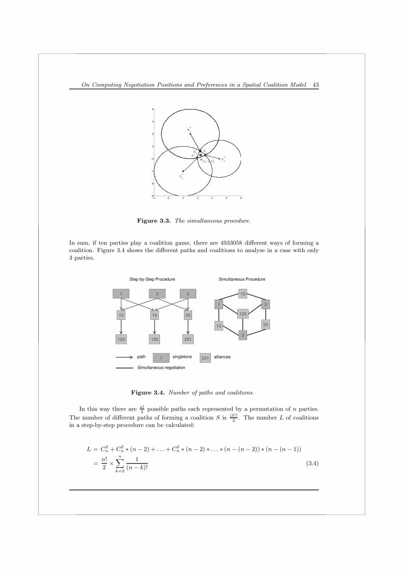
On Computing Negotiation Positions and Preferences in a Spatial Coalition Model 43
−4 −2 0 2 4 6 8−8
−6
−4
−2
0
2
4
6
x1*
x2*
x3*
x{1,2,3}
x∼2x∼
1x∼3
Figure 3.3. The simultaneous procedure.
In sum, if ten parties play a coalition game, there are 4933058 different ways of forming acoalition. Figure 3.4 shows the different paths and coalitions to analyse in a case with only3 parties.
Figure 3.4. Number of paths and coalitions.
In this way there are n!2
possible paths each represented by a permutation of n parties.
The number of different paths of forming a coalition S is |S|!2
. The number L of coalitionsin a step-by-step procedure can be calculated:
L = C2n + C2
n ∗ (n − 2) + . . . + C2n ∗ (n − 2) ∗ . . . ∗ (n − (n − 2)) ∗ (n − (n − 1))
=n!
2×
n∑
k=2
1
(n − k)!(3.4)

44 Game Theory at Work
Compared to the step-by-step procedure, the simultaneous procedure has only one pathto be followed. It models the situation where |S| parties are sitting together to come to anagreement. Besides the grand coalition, there are many possible partial-coalitions. The moreparties, the more possible coalitions can be formed. The number K of possible coalitions isgiven by:
K = C2n + C3
n + . . . + Cnn =
n∑
k=2
Ckn = 2n − (n + 1) (3.5)
Table 3.1 shows how complexity increases with the number of players (parties) in bothprocedures.
Table 3.1. Number of coalitions following different procedures.
step-by-step simultaneousNumber of parties Possible paths Number of Coalitions Number of Coalitions
2 1 1 13 3 6 44 12 30 115 60 160 266 360 975 577 2520 6846 1208 20160 54796 2479 181440 493200 50210 1814400 4932045 1013
Disregarding some special conditions, the two procedures usually lead to different po-sitions for the coalition and consequently different appreciations by the coalition members.Given the distance between the ideal position of a party and the coalition position, partieswill have a preference ranking over the different positions of the coalitions, over the differentcoalitions, and hence over the procedures to reach them. The closer a coalition agreement isto the ideal position of a party, the more this party will prefer this coalition agreement. Inthis way, we show that parties should not only form preferences over coalitions, but shouldalso take the procedure into consideration. In conclusion, the procedure of coalition forma-tion should be a strategic resource in coalition formation and should play a role in coalitionnegotiations similar to the composition of the coalition.
3.2 Algorithms for the Different Procedures
The coalition compromise differs for each different path in the step-by-step procedure. Ac-cording to the all-coalition-path configuration, one can calculate the agreement points ofall coalitions and corresponding valuations by following the procedure described in the nextsection. An index l is used to distinguish coalition. A coalition S in a step-by-step formationis an ordered subset of N . A coalition S in a simultaneous formation is a subset of N . Table3.2 summarises the notation used.

On Computing Negotiation Positions and Preferences in a Spatial Coalition Model 45
Table 3.2. Notation.
N Set of partiesi, j Index of partiesL Total number of coalitionsl coalition indexx∗
i Ideal position for party iSl A coalition, |Sl| ≥ 2, Sl ⊆ NxS
i Negotiation position of party i when coalition S is formedxS Compromise coalition position of S
xS∪{i}S Negotiation position of a coalition S when party i joins
3.2.1 Forming a Coalition Step-by-StepConsider two parties, i and j, forming a coalition S = {i, j}. By proposition 3.1 in de Ridderand Rusinowska (2005), the negotiation positions for the two parties are calculated as follows.The negotiation position for party i is: if rj < d(xi, xj),
xSi = x∗
j + rj × x∗i − x∗
j
d(x∗i , x∗
j )(3.6)
otherwise,xS
i = x∗i (3.7)
where the negotiation position of j is given by switching i and j in (3.6) and (3.7). Once theparties have defined their negotiation positions, the compromise position is calculated by
xS =wi × xS
i + wj × xSj
wi + wj(3.8)
Let S be a coalition with p members, p ≥ 1. The compromise position of the coalition isxS. If party i joins the coalition, both, the coalition S and the party i have to choose newnegotiation positions: X
S∪{i}S and x
S∪{i}i respectively. Next step is to agree on a compromise
coalition position XS∪{i}. To choose the new negotiation positions, the problem to solve is:
xS∪{i}i = arg min
z∈⋂j∈S∪{i} Mj
d(x∗i , z) (3.9)
xS∪{i}S = arg min
z∈⋂j∈S∪{i} Mj
d(XS , z) (3.10)
The compromise position for the new coalition S ∪ {i} is calculated as follows:
xS∪{i} =wi × x
S∪{i}i + X
S∪{i}S ×∑j∈S wj∑
j∈S wj + wi(3.11)
Based on the model by de Ridder and Rusinowska (2005) we introduce a procedureto determine the compromise (agreement) points and valuations of all coalitions at eachpossible path. In this procedure, (see Algorithm 3.1) first the negotiation positions and
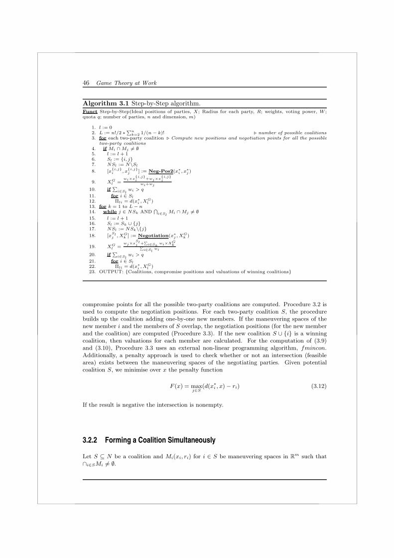
46 Game Theory at Work
Algorithm 3.1 Step-by-Step algorithm.Funct Step-by-Step(Ideal positions of parties, X; Radius for each party, R; weights, voting power, W ;quota q; number of parties, n and dimension, m)
1. l := 02. L := n!/2 ∗∑n
k=2 1/(n − k)! � number of possible coalitions3. for each two-party coalition � Compute new positions and negotiation points for all the possible
two-party coalitions4. if Mi ∩ Mj �= ∅5. l := l + 16. Sl := {i, j}7. NSl := N\Sl
8. [x{i,j}i , x
{i,j}j ] := Neg-Pos2(x∗
i , x∗j )
9. XGl =
wi×x{i,j}i +wj×x
{i,j}j
wi+wj
10. if∑
i∈Slwi > q
11. for i ∈ Sl
12. Πli = d(x∗i , XG
l )13. for k = 1 to L − n14. while j ∈ NSk AND
⋂i∈Sl
Mi ∩ Mj �= ∅15. l := l + 116. Sl := Sk ∪ {j}17. NSl := NSk\{j}18. [x
Slj , XG
k ] := Negotiation(x∗j , XG
k )
19. XGl =
wj×xSlj +
∑i∈Sk
wi×XGk∑
i∈Slwi
20. if∑
i∈Slwi > q
21. for i ∈ Sl
22. Πli = d(x∗i , XG
l )23. OUTPUT: {Coalitions, compromise positions and valuations of winning coalitions}
compromise points for all the possible two-party coalitions are computed. Procedure 3.2 isused to compute the negotiation positions. For each two-party coalition S, the procedurebuilds up the coalition adding one-by-one new members. If the maneuvering spaces of thenew member i and the members of S overlap, the negotiation positions (for the new memberand the coalition) are computed (Procedure 3.3). If the new coalition S ∪ {i} is a winningcoalition, then valuations for each member are calculated. For the computation of (3.9)and (3.10), Procedure 3.3 uses an external non-linear programming algorithm, fmincon.Additionally, a penalty approach is used to check whether or not an intersection (feasiblearea) exists between the maneuvering spaces of the negotiating parties. Given potentialcoalition S, we minimise over x the penalty function
F (x) = maxj∈S
(d(x∗i , x) − ri) (3.12)
If the result is negative the intersection is nonempty.
3.2.2 Forming a Coalition Simultaneously
Let S ⊆ N be a coalition and Mi(xi, ri) for i ∈ S be maneuvering spaces in Rm such that
∩i∈SMi �= ∅.

On Computing Negotiation Positions and Preferences in a Spatial Coalition Model 47
Algorithm 3.2 Computes negotiation positions for parties and coalition position.Funct Neg-Pos2(Ideal positions for each of the two parties: x∗
i , x∗j )
1. New position for party i2. if rj < d(xi, xj)
3. x{i,j}i = x∗
j + rj × x∗i −x∗
j
d(x∗i ,x∗
j )
4. else
5. x{i,j}i = x∗
i6. New position for party j7. if ri < d(xi, xj)
8. x{i,j}j = x∗
i + ri × x∗j−x∗
i
d(x∗i ,x∗
j )else
9. x{i,j}j = x∗
j
10. OUTPUT: {New positions for the parties and coalition position: x{i,j}i , x
{i,j}j }
Algorithm 3.3 Computes new negotiation positions for coalition and new member(party).Funct Negotiation(Ideal position for the new member i, x∗
i , of the new coalition S ∪ {i} and com-promise position of coalition S, XS)
1. objfun=objective function; objcon=objective constraints;x0=starting point2. if Mi ∩
⋂j∈S Mj �= ∅
3. xS∪{i}i = Fmincon(objfun, objcon, x0, x∗
i )
4. XS∪{i}S = Fmincon(objfun, objcon, x0, XS)
5. OUTPUT: {New negotiation positions for party i and coalition S}
1. Each party i ∈ S chooses the negotiation position xSi :
xSi = arg min
z∈⋂j∈S Mj
d(x∗i , z) (3.13)
2. Coalition position xS is chosen as gravity center of positions xSi with weights wi:
xS =
∑j∈S wjx
Sj∑
j∈S wj(3.14)
Algorithm 3.4 is the main procedure when coalitions are formed simultaneously. It com-putes the winning coalitions, its coalition positions and valuation-preferences for the parties.First, it generates all possible coalitions based on 0 − 1 notation: 0 means the party is nota member; 1 means the party is a member of the coalition. If the coalition is winning andthe maneuvering spaces of the members overlap, the algorithm calls a second procedure (Al-gorithm 3.5) to compute the negotiation positions of the members. Algorithm 3.5 uses anexternal non-linear programming algorithm to calculate the positions. Back in the main al-gorithm, the coalition position and valuations are computed in order to generate a preferenceorder.

48 Game Theory at Work
Algorithm 3.4 Simultaneous algorithm.Funct Simult(Ideal positions of parties, x∗; Radius for each party, r; weights, voting power, w; quotaq; number of parties, n and dimension, m)
1. number of possible coalitions: L := 2n − (n + 1)2. for k = 1 to L � Compute new positions and negotiation points for all the feasible coalitions3. Generate coalition Sk
4. if∑
i∈Skwk > q and
⋂i∈Sk
Mi �= ∅5. for i ∈ Sk
6. xSki := Neg-Sim(x∗)
7. XGk =
∑i∈Sk
wi×xSki∑
i∈Skwi
8. Πki = d(x∗i , XG
k )9. OUTPUT: {Coalitions, new party and negotiation positions for the simultaneous procedure}
Algorithm 3.5 Procedure to compute new negotiation positions for members incoalition S.Funct Neg-Sim(Ideal position for the party i, x∗
i )
1. objfun=objective function; objcon=objective constraints;x0=starting point2. xS
i = Fmincon(objfun, objcon, x0)3. OUTPUT: {New negotiation positions for party i}
3.2.3 Numerical Illustration
We provide an example here to illustrate how the algorithms and model work. This exampleuses the Dutch election result of 2003 (Klingemann et al. (2006)). As input for the model,we need ideal policy positions of Dutch parties, and a weight and a radius for each politicalparty. The ideal policy positions are derived from a data set with policy positions of Dutchpolitical parties on 56 dimensions from 1998 and 2003 (Klingemann et al. (2006)). Becausethe model is working with spherical maneuvering spaces based on distance calculations, thedata is all scaled between 0 and 10. The weight of the parties is determined by the amountof seats each party had in parliament (total of 150 seats). The radii that model the flexibilityof the parties is relatively arbitrary for illustrative purposes and leave a degree of freedomfor our analysis. In reality, each party has its own radius which is dependent on the specificsituation and which might be subject to change. In this case we have used similar radii forall parties. The names of the parties are the following:
CDA - Christian Democrats (Christen Democratisch Appel)CU - Christian Union (Christen Unie)D66 - Democrats 66 (Democraten ’66)GRL - Green Left (Groen Links)LPF - List Pim Fortuyn (Lijst Pim Fortuyn)PvdA - Labor Party (Partij van de Arbeid)SP - Socialist Party (Socialistische Partij)VVD - People’s Party for Freedom and Democracy
(Volkspartij voor Vrijheid en Democratie)
Note that the SGP (Political Reformed Party) is not included in this table, as it wasnot included in the dataset from Klingemann et al. (2006) (in Klingemann et al. (2006),Appendix IV, is explained that the election program for the collection of data was missing).
As output of the model, we only consider coalition positions of majority coalitions ofparties that have an overlap of their maneuvering spaces given their ideal policy positions,

On Computing Negotiation Positions and Preferences in a Spatial Coalition Model 49
Table 3.3. Data for 2003.
PartiesCDA CU D66 GRL LPF PvdA SP VVD
Radius 30 30 30 30 30 30 30 30Weight 44 3 6 8 8 42 9 28
i.e. of feasible winning coalitions. As said earlier, the biggest party gets the initiative forcoalition formation in The Netherlands. In 2003, this was the CDA. The majority coalitionswith overlapping maneuvering spaces containing CDA are included in Table 3.4. For eachcoalition reached with a certain procedure, the distance between the coalition position andthe ideal position of the party are calculated. The {PvdA, CDA} coalition leads to the samecoalition position with both procedures as no third party joins here. However, for a coalitionbetween CDA, PvdA, and LPF (e.g. {{CDA, PvdA}, LPF} and {CDA, PvdA, LPF})procedure plays a role as different procedures lead to different distances. More generally,we see in all the calculations done for this paper that procedure really makes a difference:different procedures lead to different results.
Table 3.4. Distances from ideal points for 2003 example.
Step-by-Step ProcedureCoalition Seats Distance
CU D66 GRL PvdA SP VVD LPF CDA{CDA, PvdA} 86 - - - 20.52 - - - 20.07{{CDA, PvdA}, SP} 95 - - - 24.92 29.39 - - 26.92{{CDA,PvdA},LPF} 94 - - - 25.45 - - 29.24 23.69{{CDA, SP}, P vdA} 95 - - - 26.04 29.42 - - 25.97{{CDA,LPF},PvdA} 94 - - - 25.38 - - 29.15 23.86
Simultaneous ProcedureCU D66 GRL PvdA SP VVD LPF CDA
{CDA, PvdA} 86 - - - 20.52 - - - 20.07{CDA, PvdA, SP} 95 - - - 26.01 29.00 - - 26.47{CDA,PvdA,LPF} 94 - - - 25.31 - - 28.62 24.59
Based on these distances, the preferences of the players can be calculated. The closer thecoalition position to the ideal position of a party, the more the party will prefer this coalitionand the procedure. Table 3.5 reports this. As an example, CDA’s most favorite option is tocooperate with PvdA. If CDA would cooperate with PvdA and SP, then the best procedurefor CDA would be to negotiate first with SP alone. The step-by-step procedure with SPjoining as last is CDA’s least preferred procedure for this coalition. Note that we do notconsider preferences of the parties not participating in the coalition.
In reality, the coalition that formed was {CDA, VVD, D66}. Although it is not the aimof this paper to predict which coalitions have occurred, we can explain why this coalition didnot appear in the results. According to the model and, in particular, the adopted input, thiscoalition would not be viable. That means that the adopted radii did not lead to an overlapof the parties’ maneuvering spaces; the {CDA, VVD, D66} coalition is less acceptable thanthe coalitions that appear in the table.

50 Game Theory at Work
Table 3.5. Preference order for 2003.
Step-by-Step ProcedureCoalition Seats Preference order
CU D66 GRL PvdA SP VVD LPF CDA{CDA, PvdA} 86 - - - 1 - - - 1{{CDA, PvdA}, SP} 95 - - - 2 2 - - 7{{CDA, PvdA}, LPF} 94 - - - 5 - - 3 2{{CDA, SP}, P vdA} 95 - - - 7 3 - - 5{{CDA, LPF}, P vdA} 94 - - - 4 - - 2 3
Simultaneous ProcedureCU D66 GRL PvdA SP VVD LPF CDA
{CDA, PvdA} 86 - - - 1 - - - 1{CDA, PvdA, SP} 95 - - - 6 1 - - 6{CDA, PvdA, LPF} 94 - - - 3 - - 1 4
3.3 Hypothesis TestingThe described model and introduced computational method was used in de Ridder et al.(2007) to do an extensive study to test hypotheses derived from intuition with the aid ofDutch data. The rest of this paper reports on the findings. First we formulate the hypothesesand the Dutch situation as a platform of analysis. After that we point wise discuss the resultsthat can be found in de Ridder et al. (2007).
3.3.1 Procedure: Hypothesis on First MoverEmpirical observations of how coalitions form show that procedures are in some countriesstandard and formalized in laws (e.g. Belgium, Finland, Luxembourg, and The Netherlands,Muller and Strøm (2003)). That diminishes the opportunity for parties to use procedure as astrategic means during the coalition process. An important observation is that many multi-party democracies have the (unwritten) law that the party that came out of the electionsas the largest gets the initiative (from a head of state) for forming a coalition. Examplesof countries in which this (more or less frequently) happens are The Netherlands, Sweden,Finland, Austria, Belgium, and Luxembourg (Muller and Strøm (2003)). The idea behindthis is that these initiative taking parties are supposed to lead the negotiations and tohave an advantage in the bargaining situation. The earlier a party is involved in coalitionnegotiations, the more this party is able to pull the negotiations towards its own ideas. Inthis way, this party can determine and influence the negotiations more and can get advantageout of it. This brings us to the first hypothesis: Being a first-mover in coalition negotiationsis advantageous.
3.3.2 Flexibility HypothesisThe second innovation of our model, is the flexibility during negotiations we attribute partiesvia maneuvering spaces. In the literature of coalition formation models, it has most oftenbeen assumed that political parties have a fixed position in policy space (Grofman (1982);Vries (1999)). However, more scholars begin to acknowledge the importance of studying thedynamics of party competition (Laver (2005); Timmermans (2003), van der Brug (1999)):‘...positions are not frozen or fixed; parties move in the policy space in different directionsover time’ (Timmermans (2003), p. 9). Here, we concentrate on dynamics of policy positions

On Computing Negotiation Positions and Preferences in a Spatial Coalition Model 51
not with vote maximizing as goal (as e.g. Budge (1994); Enelow and Hinich (1984); Laver(2005)), but dynamics due to coalition formation.
The idea is that in order to form a coalition, political parties will move their policyposition, but only to a certain limit (Warwick (2000)) as formalized by the maneuveringspace. Coalition formation implies making a coalition agreement: a compromise betweenthe members of a coalition on the ideological course of the coalition, consisting of a positionfor the coalition. As a consequence, parties participating in a coalition need to adjust theirposition in order to reach such an agreement (also see Martin and Vanberg (2004)). It is notlikely that parties will cooperate with a party which has opposing policy ideals. We thereforeassume parties will only be willing to compromise if they can stay within their maneuveringspace of acceptable positions.
The question now rises what is mostly in a party’s interest: a big or small maneuveringspace? When forming a two-party coalition, the answer is straightforward: being less flexibleis never disadvantageous. If a coalition consists of only two parties, the more flexible party ofthe two will be forced to move its position more than the other. One can speak of a zero-sumsituation: what one wins, is lost by the other.
Nonetheless, when forming a k-party coalition, for k ≥ 3, the answer is less easy. In-tuitively, one would consider that staying closer to a party’s ideal position is also better inmulti-party coalitions. Hence, a decrease in flexibility would always be in a party’s advan-tage. However, this is less easy to analyse due to the amount of players involved. Therefore,we use the data and theoretical results to study whether the following (second) hypothesisholds: Being less flexible in coalition negotiations is more advantageous.
3.3.3 Sharing Power: Hypothesis on Minimal Winning
As a final point, we study the role of sharing power. Coalition formation has long beenconsidered as a combination of achieving power, and simultaneously sharing this power withcoalition partners. Coalition formation is therefore a delicate balance between on the onehand getting this power by compromising into the coalition, and on the other hand, forming acoalition which gives a party relatively the best power. In this tradition, the minimal winning(von Neumann and Morgenstern (1944)) and minimum size theory (Riker (1962)) have beenformulated. Minimal winning coalitions are coalitions that contain enough members to bewinning, but are not oversized. Minimal winning coalitions cannot miss any member withoutbecoming losing. Minimum size coalitions contain enough weight to be winning, but not morethan that.
In line with this, one could reason that oversized coalitions imply sharing power with morepartners and hence compromising with more partners than necessary. The chance is biggerthat a coalition position will be reached which is farther from a party’s ideal position. Lessmembers in a coalition make it easier to reach an agreement which is closer to a party’s idealpoint. Hence hypothesis 3a: Being in a smaller (winning) coalition is more advantageousthan being in an oversized coalition.
In a similar way, we can argue that forming a coalition with a stronger partner is notadvantageous, since the stronger party may ‘pull’ the position of a formed coalition moretowards it’s own ideal position. Hence we propose hypothesis 3b: Increase of a party’s weightis disadvantageous for its coalition partners.

52 Game Theory at Work
3.3.4 Dutch Situation and DataIn The Netherlands, coalition governments are the standard, considering that the Dutchmulti-party democracy only has had coalition governments since 1945 (Muller and Strøm(2003)). Also, The Netherlands has a tradition of majority coalitions. Furthermore, two ofthe issues we highlight - procedures and flexibility - are important. Concerning procedures,the process of coalition formation is by far the longest in Western Europe with an averageof 70.6 days. This could denote an important role for procedures. The first mover issue isrelevant as it is characteristic for the Dutch coalition practice that the biggest party gets theinitiative to form a coalition. Concerning flexibility, coalition agreements play an importantrole in coalition negotiations: each cabinet agrees on such a document as the course of actionduring their period of government. Data however show different ideal policy positions ofDutch parties (e.g. Vries (1999); van der Brug (1999)) which implies compromises and henceflexibility of parties. As explained in Section 3.2, the radii that model the flexibility of theparties is relatively arbitrary for illustrative purposes and leave a degree of freedom for ouranalysis. Due to the lack of empirical data on this aspect, we have taken two different waysto determine the radius: a radius similar for each party and a radius different for each party,randomly generated. In the case (as in the case of Section 3.2) in which we have used similarradii for all parties, the radii have been determined by optimizing the case such that enough,but not too many, instances were found which could help us investigate the hypotheses.
To run the model with real-life multidimensional data, one needs computational algo-rithms. We have performed calculations with the model using data from Dutch politics, and,moreover, we present some theoretical results. Both the empirical and theoretical calcula-tions provide some counter-intuitive situations which show that certain expectations do notalways hold. Also, we illustrate that certain traditions in real-life coalition formation are notnecessarily advantageous.
During the paper, we study which strategic moves are advantageous for a potentialcoalition member. Advantageous is defined in terms of preference of a party over a coalitionand the path to reach this coalition. This is measured by taking the distance from the idealposition of the party to the position of the coalition compromise. The closer the coalitionposition, the better. The policy-distance effect on government composition, meaning thatthe incentive of a party to join a parliamentary coalition government decreases with thedistance between the policy position and the position of the government, was elaborated andtested in particular by Warwick (1998).
3.3.5 Results on ProcedureTwo different procedures of coalition formation, leading to different coalition positions, areunder study. The research question is whether being a first-mover is always advantageousfor a party in coalition negotiations, as in real-life the biggest party, after elections, is mostoften rewarded with the initiative for coalition negotiations.
In the 2003 case presented in Section 3.2, we indeed saw that for the LPF being the firstmover was advantageous. When comparing the LPF’s preference on the two step-by-stepprocedures it is involved in, it prefers {{CDA, LPF}, PvdA} over {{CDA, PvdA}, LPF}.So, it prefers being a first mover over being a late mover. A small counter example can befound due to the PvdA that in the same coalition prefers to step in later. The data of 1998and Table 3.6 show a stronger counter example, as can be observed from Table 3.7.
In the 1998 case, PvdA was the biggest party and had to take the initiative in coalitionnegotiations. For the three party coalition {PvdA, SP, CDA}, two step-by-step and onesimultaneous procedures were considered as PvdA always had to be a first mover. In the two

On Computing Negotiation Positions and Preferences in a Spatial Coalition Model 53
Table 3.6. Weights and radius 45 for 1998 data
PartiesGRL SP PvdA D66 VVD CDA
Radius 45 45 45 45 45 45Seats 11 5 45 14 38 29
Table 3.7. Preference order for 1998 data
Step-by-Step Procedure
Coalition Seats Preference orderGRL SP PvdA D66 VVD CDA
{{PvdA, SP}, CDA} 79 - 8 3 - - 2{{PvdA, D66}, CDA} 88 - - 5 7 - 4{{PvdA, CDA}, SP} 79 - 4 1 - - 7{{PvdA, CDA}, D66} 88 - - 2 4 - 8{{{PvdA, SP}, D66}, CDA} 93 - 5 10 9 - 6{{{PvdA, SP}, CDA}, D66} 93 - 1 7 8 - 9{{{PvdA, D66}, SP}, CDA} 93 - 9 11 5 - 6{{{PvdA, D66}, CDA}, SP} 93 - 7 8 1 - 10{{{PvdA, CDA}, SP}, D66} 93 - 2 6 8 - 9{{{PvdA, CDA}, D66}, SP} 93 - 7 5 2 - 10
Simultaneous Procedure
GRL SP PvdA D66 VVD CDA{PvdA, SP, CDA} 79 - 3 4 - - 1{PvdA, CDA, D66} 88 - - 9 3 - 3{PvdA, D66, SP, CDA} 93 - 6 12 6 - 5
step-by-step procedures, CDA would be better off being a late instead of a first mover. Let i denote the preference relation of party i. For this coalition, the preference order of CDAis as follows: {PvdA, SP, CDA} CDA {{PvdA, SP}, CDA} CDA {{ PvdA, CDA}, SP}.This also holds for SP, which in case of step-by-step formation rather joins as last memberin the negotiations.
We can therefore conclude that hypothesis 1 does not hold:
Result 1: Being a first mover is not always advantageous.
3.3.6 Results on FlexibilityAs a second major point, focus is on policy flexibility of parties. One of the central assump-tions of the model is that parties have maneuvering spaces which reflect their flexibility todeviate from their ideal positions. No party will accept a coalition position which lies out-side its maneuvering space. This assumption is similar to the one made in a policy-horizonmodel by Warwick (2000), (2005a), (2005b)). We study the hypothesis Being less flexible incoalition negotiations is more advantageous.
A search in the data did not provide a counter example to this hypothesis. It wasfound that a decrease in a party’s flexibility always seems to be in the party’s advantage.In other words, the intuition which was provided earlier holds. As seen more easy in two-party coalitions, less flexibility always leads to a more advantageous coalition agreement for

54 Game Theory at Work
a party. Although we did not find a counter-example in the Dutch data, we did come upwith a one-dimensional theoretical example which shows that being less flexible can be adisadvantage.
Example 1. We consider a three-party example, in which parties 1 and 2 have the sameweight, while the weight of party 3 is twice as big as the weight of party 1 and 2, i.e.
N = {1, 2, 3}, w1 = w2, w3 = 2w2
The situation is illustrated in Figure 3.5. Since this is a one-dimensional example, the idealpositions x∗
1, x∗2 and x∗
3 are points (denoted in Figure 3.5 by squares) on a line, while themaneuvering spaces M1, M2 and M3 are intervals (denoted in Figure 3.5 by two-headedarrows). We have
x∗1 = 0, x∗
2 = 4, x∗3 = −2
All parties are assumed to be equally flexible and their radii are equal to
r1 = r2 = r3 = 6
Hence, the maneuvering spaces are
M1 = [−6, 6], M2 = [−2, 10], M3 = [−8, 4]
and their intersections (also two-headed arrows)
M1 ∩ M3 = [−6, 4], M1 ∩ M2 = [−2, 6]
M2 ∩ M3 = M1 ∩ M2 ∩ M3 = [−2, 4] �= ∅.
−10 −8 −6 −4 −2 0 2 4 6 8 10 12
M3
M2
M1
M2∩ M
3 M1∩ M
2∩ M
3
M1∩ M
3
M1∩ M
2
x1*x
3* x
2*
Figure 3.5. Counter-example “being less flexible can be a disadvantage”. Ideal points(squares) and maneuvering spaces (two-headed arrows)
Since M1 ∩ M2 ∩ M3 �= ∅, the necessary condition for coalition {1, 2, 3} to be formed issatisfied. Let us consider the step-by-step procedure of forming coalition {1, 2, 3}, in whichfirst parties 1 and 2 form a coalition {1, 2}, and then party 3 joins. The steps of the procedure
are explained in Section 3.2. The negotiation positions x{1,2}1 and x
{1,2}2 of parties 1 and 2 are
equal to their ideal positions, because the ideal points lie in the intersection of the maneuveringspaces, i.e.
x{1,2}1 = 0 = x∗
1, x{1,2}2 = 4 = x∗
2
Since the weights of parties 1 and 2 are the same and the coalition position is the gravity

On Computing Negotiation Positions and Preferences in a Spatial Coalition Model 55
center of the negotiation positions, we get
x{1,2} = 2 ∈ M3
Next, party 3 joins proto-coalition {1, 2}. Because x∗3 and x{1,2} lie in the intersection of the
maneuvering spaces, the negotiation positions of party 3 and proto-coalition {1, 2} are equalto x∗
3 = −2 and x{1,2} = 2, respectively. Since the weight of party 3 is equal to the weight of{1, 2}, we get
x{{1,2},3} = 0 = x∗1
Hence, the step-by-step procedure of forming {{1, 2}, 3}, in which first parties 1 and 2 forma coalition, and then party 3 joins, leads to the coalition position x{{1,2},3} which is the bestpossible position for party 1.
Next, let us assume that party 1 becomes less flexible, that is, its new radius decreases tor′1 = 3. All remaining components of the example are unchanged. Then,
M ′1 = [−3, 3], M ′
1 ∩ M2 = M ′1 ∩ M2 ∩ M3 = [−2, 3]
We consider the same step-by-step procedure of forming {1, 2, 3} with the new radius r′1 = 3.
The new negotiation position y{1,2}1 of party 1 is the same as before (equals x
{1,2}1 ), since its
ideal point lies in the intersection of the maneuvering spaces. However, the new negotiationposition y
{1,2}2 of party 2 is different, i.e.
y{1,2}1 = x∗
1 = 0, y{1,2}2 = 3.
The new position y{1,2}, as the gravity center of y{1,2}1 and y
{1,2}2 with equal weights w1 = w2,
is now
y{1,2} =3
2∈ M3
The new coalition position y{{1,2},3}, as the gravity center of the negotiation positions y{1,2}and x∗
3 = −2, with equal weights for {1, 2} and party 3, is now
y{{1,2},3} = −1
4
Hence, the step-by-step procedure of forming {{1, 2}, 3}, in which first parties 1 and 2 forma coalition, and then party 3 joins, results now in the coalition position y{{1,2},3} which isworse for party 1 than the coalition position x{{1,2},3}, for the case where party 1 is moreflexible, i.e.
x{{1,2},3} 1 y{{1,2},3}
This means that becoming less flexible made party 1 worse off.
To conclude, although the data have shown that less flexibility always seems to be advan-tageous to a party, a theoretical counter example has illustrated how a decrease in flexibilitycan be a disadvantage for a party. Hence:
Result 2: When forming a k-party coalition, for k ≥ 3, being less flexible is usually advan-tageous, but can theoretically be a disadvantage.
3.3.7 Results on Sharing PowerAdditionally, we study a minor point: the role of sharing power. The question here is whetherstriving for a coalition in which a party gets the best relative power position is always ad-

56 Game Theory at Work
vantageous. Earlier empirical results confirm the role of power-sharing motives of parties(Martin and Stevenson (2001)), but do not show that oversized can be an advantage forcoalition members (cf. Volden and Carrubba (2004) who explain when oversized coalitionsoccur). Sub-issues here are the minimal winning argument (von Neumann and Morgenstern(1944)) and the influence of weight. The minimal winning argument states that only coali-tions will form that have enough members to be winning, but not more than that. But isa minimal winning coalition necessarily advantageous for a party? Or, more general, is asmaller coalition necessarily more advantageous than an oversized coalition?
We have found many counter-examples in Dutch data which show that the hypothesisdoes not always hold. We consider Dutch data after the 1998 elections (see Table 3.6). Here,we change the radii for the parties and let the radius be different for different parties. We getan instance as shown in Table 3.8. Table 3.9 shows the preference order for this case. Notethat under the step by step as well as simultaneous procedure, PvdA finds the non-minimalwinning coalition formed by PvdA, VVD and D66 more attractive than the minimal winningcoalition {PvdA, VVD}.
Table 3.8. Weights and different radii for 1998
PartiesGRL SP PvdA D66 VVD CDA
Radius 45 55 25 65 85 45Seats 11 5 45 14 38 29
Concluding, we get the following result.
Result 3a: Forming a minimal winning coalition is not always advantageous.
Table 3.9. Preference order with different radii for 1998
Step-by-Step ProcedureCoalition Seats Preference order
GRL SP PvdA D66 VVD CDA{PvdA, V V D} 83 - - 3 - 1 -{{PvdA, SP}, V V D} 88 - 4 12 - 5 -{{PvdA, D66}, V V D} 97 - 10 1 11 6 -{{PvdA, V V D}, SP} 88 - 8 7 - 4 -{{PvdA, V V D}, D66} 97 - 11 2 10 2 -{{{PvdA, SP},D66}, V V D} 102 - 1 8 1 12 -{{{PvdA, SP}, V V D}, D66} 102 - 2 11 2 10 -{{{PvdA, D66}, SP}, V V D} 102 - 6 5 5 12 -{{{PvdA, D66}, V V D}, SP} 102 - 9 4 7 11 -{{{PvdA, V V D}, SP},D66} 102 - 5 7 4 9 -{{{PvdA, V V D}, D66}, SP} 102 - 9 6 6 7 -
Simultaneous ProcedureGRL SP PvdA D66 VVD CDA
{PvdA, V V D} 83 - - 3 - 1 -{PvdA, SP, V V D} 88 - 7 10 - 3 -{PvdA, D66, V V D} 97 - 11 2 8 2 -{PvdA, SP, D66, V V D} 102 - 3 9 3 8 -
Concerning weight, we like to consider the consequence the weight of a party (number ofseats in parliament) has for its coalitional partners. The last research question is then: Doesan increase of a party’s weight imply a disadvantage for its coalition partners?

On Computing Negotiation Positions and Preferences in a Spatial Coalition Model 57
In a similar way, we can argue that forming a coalition with a stronger partner is notadvantageous, since the stronger party may ‘pull’ the position of a formed coalition moretowards it’s own ideal position. Hence we propose hypothesis 3b: Increase of a party’s weightis disadvantageous for its coalition partners.
One can show that forming a two-party coalition with a stronger party is never advanta-geous to the coalition partner. The intuition is that in such a ‘zero-sum’ situation, the largerparty will always be able to pull the coalition position to its own position, further away fromits partner. Nevertheless, it does not necessarily hold when forming a larger coalition. Wecan illustrate this with the following theoretical example.
Example 2. We consider the same situation as in Example 1 with party 1 being less flexible,i.e.,
N = {1, 2, 3}, x∗1 = 0, x∗
2 = 4, x∗3 = −2
r′1 = 3, r2 = r3 = 6, w1 = w2, w3 = 2w2
M ′1 = [−3, 3], M2 = [−2, 10], M3 = [−8, 4]
M ′1 ∩ M2 = M ′
1 ∩ M2 ∩ M3 = [−2, 3]
As calculated in Example 1, the coalition position y{{1,2},3} results from the step-by-stepprocedure of forming {{1, 2}, 3}, in which first parties 1 and 2 form a coalition, and thenparty 3 joins, is equal to y{{1,2},3} = − 1
4. Next, let us assume that the weight of party 1
increases: it is twice as big as the weight of party 2 and the same as the weight of party 3,i.e.,
w′1 = 2w2 = w3
The remaining components of the model remain unchanged. We consider the same step-by-step procedure of forming {{1, 2}, 3}. The new negotiation positions z
{1,2}1 , z
{1,2}2 , and
coalition positions z{1,2}, z{{1,2},3} are now the following:
z{1,2}1 = x∗
1 = 0, z{1,2}2 = 3, z{1,2} = 1 ∈ M3
z{{1,2},3} = −1
5
Comparing the distance between coalition position y{{1,2},3} and the ideal point x∗2 of party 2
and the distance between the new coalition position z{{1,2},3} and x∗2, one can conclude that
z{{1,2},3} 2 y{{1,2},3}
It means that an increase of the weight of party 1 makes party 2 better off.
This gives the following result.
Result 3b: When forming a k-party coalition, for k ≥ 3, an increase of a party’s weightmay be an advantage for its coalition partner.
In order to show a pure effect of an increase of a party’s weight in Example 2, some-what artificially we have increased the weight of party 1, keeping all remaining elementsunchanged. This is of course not what happens in a parliament, since elections (usually)preceding coalition formation fix the weights of the parties. However, it can be used byparties defining a coalition formation strategy before elections. For example, in its campaigna party may be less negative with respect to another party whose bigger size might be ben-eficial. Nevertheless, although we believe that this result is mainly of a theoretical nature,we have also constructed an instance using the data. Consider the case of Table 3.8 that

58 Game Theory at Work
presents the 1998 data with varying flexibility for the parties taking the real number of seats.The distance of the ideal of D66 to the compromise of coalition {{{PvdA, SP}, D66}, V V D}is 52.25. Let us now hypothetically assume that SP increases its weight by 30, while theother parties keep their original weights. Now the distance of the ideal of D66 to the coali-tion position becomes 51.53. This means its position improves due to an increase of anotherparty.
3.4 Conclusions
In spite of the many unwritten laws and traditions during coalition formation in countries asItaly, Luxembourg, The Netherlands, Belgium, and Ireland, political parties should be awareof the important role of the process of coalition formation. In this paper, we have shown howseveral aspects of this coalition process play an important role for the result of the coalitionnegotiations. We use a formal model of coalition formation which considers political partiesas players with ideal policy positions and maneuvering spaces denoting their flexibility todeviate from their ideal points. The output of the model is a set of feasible coalitions, whichhave a majority and whose members’ maneuvering spaces overlap. The model describeswhich coalition position will be reached by the members given the procedure adopted. Thecomplexity of the model increases with the number of players (parties) and policy dimension.
To generate coalitions from political data, algorithms have been presented. We haveintroduced computational algorithms for the different procedures. The algorithms computeall winning coalitions and preferences of parties over those coalitions. Furthermore, thealgorithms are used to test different hypotheses.
The analysis in de Ridder et al. (2007) focused on three aspects of coalition formation andformulated hypotheses: procedure, flexibility, and power sharing. The following questionswhich political parties may (and should) take into account when forming a coalition wereunder study: Does procedure of coalition negotiations matter? Is it more advantageous tobe a first-mover in the coalition process? Is it better to be more or less flexible in coalitionformation? Should we invite more parties to join to a (minimal) winning coalition or is itbetter to stay with the existing one(s)? Is it better to form a coalition with a stronger partyor rather with a smaller one? Applying the algorithms to Dutch data and using theoreticalresults, we have arrived at several (counter-)examples. These counter-examples have shownthe importance of the process and give important implications for political parties involvedin coalition formation. Also, these results have implications for future coalition research.
From the output of the applied methods the following can be observed. First, procedurematters. When forming a coalition, political parties should be aware of the important roleprocedure plays in determining the result of the coalition. The calculations have shown thatprocedure partly determines which coalition point is agreed on. However, earlier research hasanalyzed that there is not one procedure which is always best (de Ridder and Rusinowska(2005)).
Related to procedure, being a first mover is not necessarily advantageous. This resultis also surprising in the sense that in many countries (e.g. The Netherlands, Belgium,Luxembourg, and Austria) the tradition is that the largest party can start the negotiationsand determines who will negotiate first. Being involved early in the process is consideredan advantage. However, from the model it appeared that this is not always the case. Therationale here is that, by studying coalition compromises the other coalition partners willreach without a party (assuming complete information), this party can estimate whether thiscompromise is close to its ideal position. If it is, it may pay to join later. If the compromise

On Computing Negotiation Positions and Preferences in a Spatial Coalition Model 59
is not close, it may be better for the party to join earlier in the process.With respect to flexibility, being less flexible is not necessarily advantageous. In the
data, we have found that being less flexible results in a (pre-)coalition compromise which iscloser to a party’s position. So, being less flexible pays off. Nevertheless, we have presenteda theoretical three-party counter-example in which being less flexible is a disadvantage. Inthis example, the first mover’s ideal position was somewhere between the ideal position ofthe remaining two parties. Although being less flexible gave a better pre-coalition outcome,the final coalition position was worse for the party than the coalition position with the partybeing more flexible.
Related to power sharing theories (as minimal winning theory), computations show thatforming a minimal winning coalition is not necessarily advantageous. Moreover, forming acoalition with a stronger party is not necessarily disadvantageous. So, it might pay off toshare power with more and stronger parties than predicted by power sharing theory. Toexplain this counter-intuitive finding, for the minimal winning case it holds that new partiesmay determine a final coalition outcome closer to a party’s ideal position, although thisdepends on the ideal positions of the new parties. For the stronger partner case, a strongerparty joining usually moves the pre-coalition compromise further from a party’s own idealposition. However, a strong party may determine a final coalition position which is closer toa party’s position. In that case, a strong partner may be beneficial to cooperate with.
Game theoretic models like the coalition formation model allows analysis only for fewplayer situations. The developed computational methods allow empirical testing of hypothe-ses using huge data sets with many players. We have provided theoretical examples andempirical cases which confirm the thesis that the coalition process matters. We aim toreach the agenda of coalition research with this message. Due to the focus on making andillustrating this message, we have neglected other aspects of the research. We suggest forfuture research to investigate how to empirically determine a party’s flexibility, developmentof more dynamic coalition models, and empirical analyses of more countries.


CHAPTER 4
Methods for Computing NashEquilibria of a Location-Quantity
Game
Chapter based on article: Saiz, M.E., Hendrix, E.M.T.(2007), Methods for computing Nash
equilibria of a location-quantity game, Accepted by Computers & Operations Research
in Press: doi:10.1016/j.cor.2007.02.022
Abstract
A two stage model is described where firms take decisions on where to locate their facility andon how much to supply to which market. In such models in literature, typically the marketprice reacts linearly on supply. Often two competing suppliers are assumed or several thatare homogeneous, i.e. their cost structure is assumed to be identical. The focus of thispaper is on developing methods to compute equilibria of the model where more than twosuppliers are competing that each have their own cost structure, i.e. they are heterogeneous.Analytical results are presented with respect to optimality conditions for the Nash equilibriain the two stages. Based on these analytical results, an enumeration algorithm and a localsearch algorithm are developed to find equilibria. Numerical cases are used to illustrate theresults and the viability of the algorithms. The methods find an improvement of a resultreported in literature.

62 Game Theory at Work
4.1 Introduction
Many studies in literature describe a so-called non-cooperative game where competing firmsdecide on production locations and supply quantities to markets. To make a game theoreticanalysis tractable, often a limited number of suppliers are considered, or alternatively homo-geneous firms and markets are assumed. We focus on situations where companies can be aswell similar as not similar. In supply chains, farm cooperatives, etc., many decisions appearin which preferences cannot be assumed to be homogeneous. Also symmetric behaviour,finite strategy set or a two or few actors setting are strong assumptions in literature. De-cisions are influenced by differences on prices or cost (“player” depending) between actorsand between the location of the facilities. Our focus is on constructing solution methodsfor games in which players are: asymmetric, heterogeneous and facing multiple decisions inseveral stages.
Different competitive location models are available in the literature, see for instancethe survey papers Eiselt and Laporte (1996), Eiselt et al. (1993), Plastria (2001) and thereferences therein. They vary in the ingredients which form the model. For instance, thelocation space may be the plane, a network or a discrete set.
In Cournot (1838) the idea of a Cournot oligopoly equilibrium was introduced, wheretwo firms compete on the same market. Due to price reaction of the market on the totalquantity offered, a price equilibrium appears. Hotelling (1929), added the idea of having afreedom in choice of location, where the possible location area is a simple line in betweenthe markets. A generally applicable concept is that of a Nash equilibrium, Nash (1951),which is defined by the situation where none of the firms (players) is better off by changingits current (equilibrium) strategy. Because choice of location is usually prior to decision onquantities, in the model under consideration, this concept is applied to a supply chain studywhere two nested levels of decisions are at stake: that of supply quantity and location choice.The corresponding solution concept adopted is that of a subgame perfect Nash equilibrium,(Selten (1975)).
The basis of the model has been introduced by Bulow et al. (1985) who consider a gamewith 2 markets and 2 firms. Later, Farrell and Shapiro (1990) studied a game on quantitydecisions with one market and n firms where decisions are simultaneous and products arehomogeneous. Labbe and Hakimi (1991) consider a two-stage location-quantity simultaneousgame with m markets and 2 firms with linear demand. Sarkar et al. (1997) extend theseresults considering a 2-stage static and simultaneous game with m markets and n firms ina network. They only consider a case with a fixed number of firms entering in the market,i.e., the quantities offered by each firm in all markets are strictly positive. Rhim et al.(2003) extend the work in Sarkar et al. (1997) by considering free entry (simultaneous andsequential) with symmetric cost (site specific) and capacity limitations. Their setting is a 3-stage game with m markets and n firms with production capacity and quantity decisions, andfinal stage is the location choice in a network. Recently, Dorta-Gonzalez et al. (2004) applythe Stackelberg equilibrium in a two-stage non-cooperative Cournot game with location andquantity choice with n markets located at the vertices of a network and r firms. They usethe Nash equilibrium concept in the location stage. In all of these studies, cases applied aresmall, most are symmetric, and no computational experience is reported.
This paper extends the studies in Sarkar et al. (1997) and Rhim et al. (2003). A two-stage location-quantity game with m markets and n firms is described. The location spaceis a network, where the nodes are considered as possible locations for the firms. Free entry ispossible as in Rhim et al. (2003), i.e., the number of firms entering the markets is not knownin advance, but in our case costs are asymmetric (firm-specific). We provide conditions forthe supplying decisions (second-stage of the game). Moreover, as firms will be affected by

Methods for Computing Nash Equilibria of a Location-Quantity Game 63
the timing and level of entry on the market, properties on how to determine the size of themarket are derived. Another difference with the study of Rhim et al. (2003) is the procedureon how to find the equilibrium of the game. We consider not only the possibility of leavinga market but also the possibility of that the supplier moves its facility to another location.Doing so, a firm has to re-think the quantity decision on how much to supply to whichmarkets. By applying the method in the cases of Sarkar et al. (1997), a mistake is found inthe outcome given in their study. Their reported possible equilibrium appears to be wrong asis shown in Section 4.4. Moreover, a sequential analysis is followed in this paper. It appearsthat starting with the cheapest firm, one can successively arrive at the size of each of themarkets. When market sizes are determined, the optimum quantities each supplier deliversto each markets they enter can be computed.
In Section 4.2, a model is outlined consisting of a non-cooperative game where quantitydecisions and location decisions take place. Furthermore, theoretical results concerning theoptimum decisions in these models are derived. In Section 4.3, methods for computing theNash equilibria on quantity-location decisions and for computing the size of a market aredescribed. A complete enumeration algorithm and a local search procedure are outlined.Numerical illustrations of model and methods can be found in Section 4.4. Finally, Section4.5 discusses the conclusions.
4.2 Location-Quantity Game: Problem FormulationThe model describes a two-stage non-cooperative game. In the first stage of the game, firmstake a simultaneous decision about where to locate a supplying facility in a network, i.e.,each firm chooses a location-strategy without knowledge of the strategy chosen by the otherfirms. In the second stage of the game, firms decide about the quantity to be produced atthese facilities and how much to supply to each market.
The model on quantity decisions and location choice is described by the following no-tation. Firms are denoted by an index i ∈ N = {1, . . . , n} and markets are denoted by anindex h ∈ M = {1, . . . , m} each demanding a quantity of a good, depending on its price. Ingame theory, usually a linear price reaction model is assumed. We will follow this tradition.The demand is fulfilled by the supply of a quantity Qih from the facility of firm i to marketh. The location xi of the facility of firm i determines its marginal production cost ci(xi).The regional dispersion effect comes in when every market appears to be situated at onelocation and, an important assumption, each supply firm can open a facility at only one ofthe locations. The relations are formalised as follows.
Let G = (V, E) be an undirected graph with V and E as its sets of nodes and edgesrespectively, |V | = m. Given two nodes vi, vj ∈ V , d(vi, vj) is the length of a shortest (withrespect to the sum of edge lengths) path on G connecting vi and vj . There are m marketslocated each at one node on the network ; there are n firms that open a facility each atone node with n ≤ m. Let xi ∈ V = {v1, . . . , vm} be the location decision by firm i onthe network. The cost of establishing a facility by firm i at xi is w(xi) ≥ 0. The quantitydecision matrix Q for all firms and all markets is given by:
Q =
⎛
⎜⎜⎜⎜⎝
Q11 . . . Q1h . . . Q1m
. . . . . . . . . . . .Qi1 . . . Qih . . . Qim
. . . . . . . . . . . .Qn1 . . . Qnh . . . Qnm
⎞
⎟⎟⎟⎟⎠

64 Game Theory at Work
where the sum of a row indicates the quantity supply by firm i over all markets h ∈{1, . . . , m}, si =
∑mh=1 Qih and the sum of a column indicates the quantity supplied by
all firms i ∈ {1, . . . , n} to market h, qh =∑n
i=1 Qih. The price ph(qh) at market h isassumed to depend on the quantity according to the relation:
ph(qh) = max{0, αh − βhqh}, qh ≥ 0 (4.1)
with price parameters αh ≥ 0, βh > 0. Notice that αh is the price when quantity offered iszero, and βh is the price reaction parameter of the inverse demand function. The price atmarket h depends on the quantity decision of all firms that supply to market h.
The n firms interact over two stages. In the first stage, firms simultaneously choose thelocations of their facilities, xi, i = 1, . . . , n, vector X = (x1, . . . , xn) gives the location of thefirms. In the second stage, depending on the location decisions xi, firms choose quantitiesQih to be supplied to markets, which results in the quantity decision matrix Q. The profitfirm i wants to maximise is denoted by πi(xi, Q). A strategy for firm i at market h, [xi, Qih],comprises a choice of xi for stage 1 and a choice of Qih for stage 2; a strategy [xi, Qi·], forall markets, where Qi· denotes the row vector (Qi1, . . . , Qim).
The game is solved backwards. First the second stage is solved. Firm i chooses optimallythe vector of quantities Qi· = (Qi1, . . . , Qim), based on what the others deliver and dependingon the chosen location xi:
Q∗i· = arg max
Qi·πi(xi, Q
∗(X)) (4.2)
The game can be considered a one stage problem when matrix Q∗ is defined for each locationvector X. Now firm i chooses a location strategy x∗
i such that:
x∗i = arg max
xi
πi(xi, Q∗(X))
The unit transportation cost between the location xi of the facility of firm i and location vh
of market h, is represented by tih = T (d(xi, vh)), where T is concave and increasing in thedistance1. The total cost of the location and supply decision of firm i is given by:
TCi(xi, Qi·) =m∑
h=1
tihQih + ci(xi)si + w(xi)
=m∑
h=1
tihQih + ci(xi)m∑
h=1
Qih + w(xi)
=m∑
h=1
(tih + ci(xi))Qih + w(xi)
For the convenience of notation we represent the total unit cost of firm i at market h by
TCuih = tih + ci(xi).
1This assumption also appears on the studies of Lederer and Thisse (1990), Labbe and Hakimi(1991), Sarkar et al. (1997) among others

Methods for Computing Nash Equilibria of a Location-Quantity Game 65
Profit is denoted by πi and defined as:
πi(xi, Q) =m∑
h=1
ph(qh)Qih − TCi(xi, Qi·) (4.3)
Price at market h is given by equation (4.1). Firms determine quantities for the markets tomaximize profit. Substituting the price relation of the markets into (4.3) gives
πi(xi, Q) =m∑
h=1
max
[αh − βh
n∑
j=1
Qjh, 0
]Qih − TCi(xi, Qi·) (4.4)
Table 4.1 summarises the notation used.
Table 4.1. Notation
N, M Set of firms and markets, respectivelyxi Location of firm ivh Location of market hQih Quantity supply by firm i at market hQi· = (Qi1, . . . , Qim) Quantity decision vector for firm isi =
∑h∈M Qih Total quantity supplied by firm i
qh =∑
i∈N Qih Total quantity supply at market hαh, βh Price parametersph(qh) = max{0, αh − βhqh}, qh ≥ 0 Price at market htih = T (d(xi, vh)) Unit transportation costw(xi) Cost of establishing a centre at xi
ci(xi) Marginal production costTCuih = tih + ci(xi) Total unit costTCi(xi, Qi·) Total cost of location and supplyπi(xi, Q) Profit for firm i depending on location and quantities
In Section 4.2.1, properties are given of the equilibrium prices and quantities dependingon the location decision of the firms. Section 4.2.2 describes the criterion for selecting optimallocation decisions, X∗, based on the optimal quantity decisions, Q∗(X).
4.2.1 Quantity Decision
The Nash equilibrium is the solution concept used in the quantity-stage of the game. From(4.2), the Nash elements of the Q matrix can be determined by an iterative process. Nashequilibrium quantities shipped by firm i to market h follow from the first order conditionoptimising (4.4) over Qih:
Q∗ih = max
{0,
αh − βh
∑nj=1,j �=i Q∗
jh − tih − ci(xi)
2βh
}(4.5)
This means that the equilibrium quantity Q∗ih can be either 0 or positive. In the remaining
we will study for which firms the quantity Q∗ih is positive and derive the exact quantity.
First, we distinguish for each market h between two groups: Ah with firms delivering to h,

66 Game Theory at Work
Q∗ih > 0; and Ah = N\Ah with firms not delivering to h, Q∗
ih = 0.
{Q∗
ih > 0 for i ∈ Ah
Q∗ih = 0 for i ∈ Ah
Proposition 1 provides the equilibrium quantity for each firm i ∈ Ah.
Proposition 1. Let Ah be the set of firms which supply market h, |Ah| = kh. The positive
equilibrium quantities are given by
Q∗ih =
αh − kh(ci(xi) + tih) +∑
j∈Ah\{i}(cj(xj) + tj)
(kh + 1)βh(4.6)
with Q∗ih > 0 ∀i ∈ Ah. Q∗
ih depends on production and transportation cost of the active
suppliers.
Proof. From equation (4.5) follows for i ∈ Ah
Q∗ih =
αh − tih − ci(xi)
2βh− 1
2
∑
j∈Ah\{i}Q∗
jh (4.7)
Let aih = (αh − tih − ci(xi)) / (2βh), then (4.7) can be written as
Q∗ih = aih − 1
2
∑
j∈Ah\{i}Q∗
jh
In vector notation
⎛
⎜⎜⎜⎜⎜⎜⎜⎜⎜⎜⎝
Q∗1h
. . .
Q∗ih
. . .
Q∗khh
⎞
⎟⎟⎟⎟⎟⎟⎟⎟⎟⎟⎠
=
⎛
⎜⎜⎜⎜⎜⎜⎜⎜⎜⎜⎝
a1h
. . .
aih
. . .
akhh
⎞
⎟⎟⎟⎟⎟⎟⎟⎟⎟⎟⎠
− 1
2
[1kh
1′kh
− I]
⎛
⎜⎜⎜⎜⎜⎜⎜⎜⎜⎜⎝
Q∗1h
. . .
Q∗ih
. . .
Q∗khh
⎞
⎟⎟⎟⎟⎟⎟⎟⎟⎟⎟⎠
Q∗h
= ah − 1
2
[1kh
1′kh
− I]Q∗
h
where 1khis the all ones vector and I is the kh × kh unit matrix. By linear algebra,
IQ∗h
= ah − 1
2
(1kh
1kh
′ − I)
Q∗h

Methods for Computing Nash Equilibria of a Location-Quantity Game 67
ah =1
2
[1kh
1′kh
+ I]Q∗
h
then, Q∗h
can be written as
Q∗h
= B−1ah (4.8)
where B is the kh × kh matrix
B =1
2
[1kh
1′kh
+ I]
having the following form,
B =
⎛
⎜⎜⎜⎜⎜⎜⎜⎜⎜⎜⎜⎜⎜⎜⎜⎜⎝
1 . . . 1/2 . . . 1/2
. . . . . . . . . . . . . . .
. . . . . . . . . 1/2 . . .
1/2 . . . 1 . . . 1/2
. . . 1/2 . . . . . . . . .
. . . . . . . . . . . . . . .
1/2 . . . 1/2 . . . 1
⎞
⎟⎟⎟⎟⎟⎟⎟⎟⎟⎟⎟⎟⎟⎟⎟⎟⎠
The inverse matrix can be derived to be,
B−1 = 2
(I − 1
kh + 11kh
1′kh
)
B−1 = 2
⎛
⎜⎜⎜⎜⎜⎜⎜⎜⎜⎜⎜⎜⎜⎜⎜⎜⎝
kh/kh + 1 . . . −1/kh + 1 . . . −1/kh + 1
. . . . . . . . . . . . . . .
. . . . . . . . . −1/kh + 1 . . .
−1/kh + 1 . . . kh/kh + 1 . . . −1/kh + 1
. . . −1/kh + 1 . . . . . . . . .
. . . . . . . . . . . . . . .
−1/kh + 1 . . . −1/kh + 1 . . . kh/kh + 1
⎞
⎟⎟⎟⎟⎟⎟⎟⎟⎟⎟⎟⎟⎟⎟⎟⎟⎠

68 Game Theory at Work
The equivalence of equations (4.5) and (4.6) for each market h now follows from (4.8):
Q∗h
= B−1ah = 2
[I − 1
kh + 11kh
1′kh
]ah =
= 2
⎛
⎜⎜⎜⎜⎜⎜⎜⎜⎜⎜⎜⎜⎜⎜⎜⎜⎝
kh/kh + 1 . . . −1/kh + 1 . . . −1/kh + 1
. . . . . . . . . . . . . . .
. . . . . . . . . −1/kh + 1 . . .
−1/kh + 1 . . . kh/kh + 1 . . . −1/kh + 1
. . . −1/kh + 1 . . . . . . . . .
. . . . . . . . . . . . . . .
−1/kh + 1 . . . −1/kh + 1 . . . kh/kh + 1
⎞
⎟⎟⎟⎟⎟⎟⎟⎟⎟⎟⎟⎟⎟⎟⎟⎟⎠
⎛
⎜⎜⎜⎜⎜⎜⎜⎜⎜⎜⎝
a1h
. . .
aih
. . .
akhh
⎞
⎟⎟⎟⎟⎟⎟⎟⎟⎟⎟⎠
and for each firm i we obtain:
Q∗ih =
2kh
kh + 1aih − 2
kh + 1
∑
j∈Ah\{i}ajh
=2kh
kh + 1
αh − tih − ci(xi)
2βh− 2
kh + 1
∑
j∈Ah\{i}
αh − (tjh + cj(xj))
2βh
=2khαh − 2kh(tih + ci(xi))
2(kh + 1)βh− (kh − 1)αh
(kh + 1)βh+
∑
j∈Ah\{i}
tjh + cj(xj)
(kh + 1)βh
=αh − kh(tih + ci(xi)) +
∑j∈Ah\{i}(tjh + cj(xj))
(kh + 1)βh
which corresponds to equation (4.6).
Consequently, the total quantity supplied to market h is:
q∗h =∑
j∈Ah
Q∗jh =
1
(kh + 1)βh
⎛
⎝khαh −∑
j∈Ah
(cj(xj) + tjh)
⎞
⎠ (4.9)
which means that higher average marginal cost and transportation costs decrease the totalquantity supplied. The optimal price at each market can now be derived by substituting(4.9) into (4.1):
p∗h =
1
kh + 1
⎛
⎝αh +∑
j∈Ah
(cj(xj) + tjh)
⎞
⎠ (4.10)
Optimal prices at each market proportionally rise with average marginal cost and transporta-

Methods for Computing Nash Equilibria of a Location-Quantity Game 69
tion cost over the firms supplying the market. Higher costs leads to a higher equilibriumprice and lower costs leads to higher quantity supplied.
In order to have any delivery at market h in (4.9) a necessary condition is that ∃j ∈ Nsuch that TCujh < αh. From Proposition 1 also follows the result for the symmetric case.
Theorem 1. Let unitary costs be symmetric (the same) for all the suppliers at market h.
If unitary costs are lower than αh, all the suppliers will enter the market.
Proof. Let the n firms entering the market have the same cost, TCu1h = TCu2h = . . . =
TCunh = Cuh and Cuh < αh, the optimal quantity and price can be derived from equation
(4.6) and (4.10),
Q∗ih =
αh − nTCuih +∑n
j=1,j �=i TCujh
(n + 1)βh=
αh − Cuh
(n + 1)βh> 0
and
p∗h = αh − βhqh = αh − βhn
αh − Cuh
(n + 1)βh=
αh + nCuh
n + 1
Corollary 2. Let unitary costs be symmetric (the same) for all the suppliers at market h.
If unitary costs are higher than αh, no suppliers will enter the market.
From Proposition 1 can also be derived when a firm would be interested to enter marketh, given that a set of firms Ah is already delivering.
Proposition 2. Let Ah be a set of firms supplying market h. A firm i is interested in
supplying market h if TCuih < p∗h.
Proof. Follows from the partial derivative of πi with respect to Q∗ih for Q∗
ih = 0.
Proposition 3. In the optimum Q∗, ∀i ∈ Ah, TCuih < p∗h.
Proof. From equation (4.10) the equilibrium price is
p∗h =
1
kh + 1
⎛
⎝αh +∑
j∈Ah
(cj(xj) + tjh)
⎞
⎠ =1
kh + 1
⎛
⎝αh +∑
j∈Ah
TCujh
⎞
⎠

70 Game Theory at Work
From equation (4.6) equilibrium quantities are given by
Q∗ih =
αh − kh(ci(xi) + tih) +∑
j∈Ah\{i}(cj(xj) + tj)
(kh + 1)βh
=αh − khTCuih +
∑j∈Ah\{i} TCujh + TCuih − TCuih
(kh + 1)βh
=αh − (kh + 1)TCuih +
∑j∈Ah\{i} TCujh + TCuih
(kh + 1)βh
=αh − (kh + 1)TCuih +
∑j∈Ah
TCujh
(kh + 1)βh
=αh +
∑j∈Ah
TCujh
(kh + 1)βh− (kh + 1)TCuih
(kh + 1)βh
=p∗
h
βh− TCuih
βh=
p∗h − TCuih
βh
From equation (4.6), at equilibrium Q∗ih > 0 ∀i ∈ Ah, (p∗
h − TCuih) /βh > 0 such that
p∗h > TCuih.
Consequently, for i ∈ Ah
ci(xi) + tih <1
|Ah| + 1
⎛
⎝αh +∑
j∈Ah
[cj(xj) + tjh]
⎞
⎠
For all j /∈ Ah, Q∗jh = 0 and
cj(xj) + tjh ≥ 1
|Ah| + 1
⎛
⎝αh +∑
i∈Ah
[ci(xi) + tih]
⎞
⎠
Proposition 4. The relation between the firm with the highest total unit costs in the active
set, i ∈ Ah, with any firm j ∈ Ah which is not entering the market is
TCuih <αh +
∑r∈Ah
TCurh
|Ah| + 1≤ TCujh
Proof. The first inequality follows from TCuih < ph and is satisfied by any firm in the active
set Ah. The last inequality is satisfied by any firm j ∈ Ah following from TCujh ≥ ph.
Proposition 4 shows that
maxi∈Ah
TCuih < ph ≤ minj∈Ah
TCujh
This is used in the algorithms in Section 4.3 to determine the number of active firms |Ah|.
Methods for Computing Nash Equilibria of a Location-Quantity Game 71
Firms are ordered on the basis of total unit costs, such that TCu(1)h ≤ TCu(2)h ≤ . . . ≤TCu(n)h. The rule that is used is the following
1. Initialise p = α, |A| = 0.
2. while TCu(k) < p, (k) enters the market and the price is updated.
More details of the algorithms are given in Section 4.3.
Let Mi be the set of markets in which firm i is active, Mi = {h ∈ M |i ∈ Ah}. The totalquantity supplied by each firm is
si =∑
h∈Mi
Q∗ih =
∑
h∈Mi
αh − kh(ci(xi) + tih) +∑
j∈Ah\{i}(cj(xj) + tjh)
(kh + 1)βh
Total cost for each firm is
TCi =∑
h∈Mi
(ci(xi) + tih)αh +
∑j∈Ah\{i}(cj(xj) + tjh) − kh(ci(xi) + tih)
(kh + 1)βh+ w(xi)
Using (4.6) and (4.9), the final payoff for each firm given location vector X is:
πi(X) =∑
h∈Mi
(p∗h − (ci(xi) + tih)Q∗
ih − w(xi)
=∑
h∈Mi
[αh +
∑j∈Ah
(cj(xj) + tjh) − (kh + 1)(ci(xi) + tih)]2
(kh + 1)2βh− w(xi)
=∑
h∈Mi
[αh +
∑j∈Ah\{i}(cj(xj) + tjh) − n(ci(xi) + tih)
]2
(kh + 1)2βh− w(xi)
=∑
h∈Mi
βh(Q∗ih)2 − w(xi)
Concluding, the optimum Q∗ih, q∗h and p∗
h in equation (4.6), (4.9) and (4.10), respectively, isa Nash Equilibrium for the competitive second stage of the game given location vector X.
4.2.2 Location Decision
Given the optima of the second stage, focus is on the first stage of the game. Considering theequilibrium supply quantity choice in the second stage, Q∗(X), each firm i maximizes theprofit function πi by selecting a location on the network. Firms locate at one of the nodes ofthe network. We assume that several firms can be located at the same site. At equilibrium,no other location decision is better off for each firm.
The strategy X∗ = (x∗1, . . . , x
∗n) is a Nash Equilibrium if for each firm i, x∗
i is the bestresponse to the strategies specified by the n − 1 other firms:
πi(x∗i , Q
∗(X∗)) ≥ πi(xi, Q∗(X)) with X = (x∗
1, . . . , xi, . . . , x∗n) ∀ xi

72 Game Theory at Work
for every feasible strategy xi. That is, x∗i solves
maxxi
πi(xi, Q∗(X))
The method and algorithms used to select optimal locations and quantities for the firms aredescribed in Section 4.3.
4.3 Methods for Computing Nash Quantities and Nash LocationsThe results of Section 4.2 can be used to find equilibria of the two level game. A procedureis described that solves the quantity game given a location configuration. This procedurecan be used in algorithms to find equilibria for the location decision. The idea is to do aglobal search to find all Nash equilibria.
Global search methods include complete (enumerative) search strategies and stochasticsearch algorithms (e.g., pure random search and multistart, see Hendrix (2007)).
First, we describe an algorithm that systematically enumerates all location possibilities,for which equilibrium quantities are computed. After that, it tries to detect which locationvectors correspond to a Nash equilibrium by checking whether it is better for a firm torelocate its facility. Notice that all mn location configurations are generated. This is calleda full enumeration.
Second, a multistart algorithm based on an application of Teitz and Bart location-allocation heuristic is described (see Teitz and Bart (1968))2. Efficiency and effectivenessare discussed in comparison to the complete enumeration algorithm.
Algorithm 4.1 Algorithm for searching Nash equilibria.Funct MAIN(Number of firms n; number of markets m; parameters α and β ; distance matrixd(vi, vj); marginal costs ci(xi), opening costs w(xi))
1. all possible locations: L← mn
2. Generate location matrix with rows Xl iteratively3. for each location l4. Q∗
l := Quantity(Xl)5. Π∗
l := Profit(Xl, Q∗l )
6. E∗ := Equilibria(Π∗)7. OUTPUT: {Nash equilibria of the non-cooperative game}
The enumeration algorithm is sketched in“Algorithm for searching equilibria”(Algorithm4.1) which calls iteratively to a subroutine called Quantity. This procedure computes theNash equilibrium quantities for each location vector based on the size of the market andequilibrium price (line 4 in Algorithm 4.1). Once the optimal quantities have been deter-mined, the subroutine called Profit computes the profit for the firms at all the possiblelocation vectors based on Nash quantities (line 5). The output is the profit (payoff) ma-trix Π. Finally, a subroutine determining the Nash equilibria on location decisions, calledEquilibria (line 6), is described.
Procedure Quantity for computing Nash equilibrium on QuantitiesProcedure Quantity is called by Algorithm 4.1 for each of the possible location vectors for
2We thank an anonymous referee for inviting us to consider this algorithm

Methods for Computing Nash Equilibria of a Location-Quantity Game 73
the suppliers. Every time the procedure is called, total unit costs are computed for eachfirm at each market and ordered, TCu(1)h, . . . , TCu(n)h (Sort in line 3). Results derived inSection 4.2.1 are applied to compute optimal quantities. The computation generates theseby the following two procedures:
Algorithm 4.2 Quantity(X) : Procedure to compute Nash equilibrium quantities,Q∗.Funct Quantity(location vector X and global variables)
1. for h ∈M2. TCu·h := t·h + c(X) � Total unit cost3. STCu·h := Sort(TCu·h) � Order the firms on total unit costs4. [kh, ph] := SizeMarket(STCu·h, αh, kh, ph, Ah)5. Q∗
·h := OptQ(STCu·h, ph, αh, βh, kh, Ah)6. OUTPUT: {Nash equilibrium Quantity decisions: Q∗}
1. Procedure SizeMarket (Algorithm 4.3): this procedure determines the size of theactive set Ah (Proposition 4) and the equilibrium price p∗
h;
2. Procedure OptQ (Algorithm 4.4): this procedure computes optimal quantities for firmsentering the market h. From equation (4.6) (Proposition 1) and depending on theasymmetry of the firms, the method finds the optimal quantities for the active firms.
Algorithm 4.3 SizeMarket(TC, α, k, p, A): Procedure to determine the size k ofmarket h and equilibrium price p.Funct SizeMarket(Total unitary costs TC, α)
1. p := α � Initial price at the market2. k := 0 � Initial size of the market3. while k ≤ n and TCk+1 < p4. k := k + 1
5. p :=α+
∑kj=1 TCj
(k+1)
6. OUTPUT: {Size and price of market h: k, p; and active set, A}
Algorithm 4.4 OptQ(TC, p, α, β, k, A): Procedure to compute the optimal quantitiesfor firms at market h.Funct OptQ(Total unitary costs TC,price at market, p, parameters α, β and size of the market, k,active set, A)
1. if k == 02. Q := 0 ∀i3. else4. for i ∈ A
5. Qi :=α−(k+1)TCi+
∑kj=1 TCj
(k+1)β
6. for i ∈ A = N\A7. Qi := 08. OUTPUT: {Optimal quantities: Q∗}
Algorithm Location StageIn the location-stage, the problem is to maximize profit by selecting a node where to locate

74 Game Theory at Work
the facility in the network. Given n supplier firms and m markets, the feasible set X hasL = mn elements. A Nash equilibrium can be identified for the first stage game by testingeach element of X in the following way. Consider location vector Xl = (xl1, . . . , xli, . . . , xln).Note that it is possible that xli = xlj for i �= j ∈ N . For each firm, one should test whetherfirm i located at xli is better off leaving its current location choosing another, xki ∈ V withk �= l and k ≤ L. For this, one should check the profit of the firm at another locationconfiguration which is in the so-called neighbourhood of Xl. The concept of neighbourhoodin this context has been introduced in Saiz et al. (2006). This step generates a set ofpossible configurations where only firm i has a different location with respect to Xl (step 4in Algorithm 4.5). The firm knows that its decision could generate changes in the quantitychoice by the other supplier firms. If none of the other locations is profitable for firm i, thisfirm is so-called “at equilibrium” with respect to its current location decision, xli. As valuesof n and m are given in the input of the algorithm, the set of feasible locations is finite andthe search process stops with an optimum, equilibrium, if it exists.
If firm i finds a location xki ∈ V, xki �= xli, in which it is better off than at xli, thenlocation vector Xl = (xl1, . . . , xli, . . . , xln) is not at equilibrium. Firm i will prefer to moveand to locate its facility at xki. The procedure follows with another possible vector locationwith all the possible deviations, i.e. from its neighbourhood. If no firm j improves by movingto another site from xlj (∀j ∈ N), then Xl is at equilibrium. The procedure proceeds checkingall possible location vectors one by one whether or not it is a Nash equilibrium. In this way,all Nash equilibria (if many) are found by the complete enumeration algorithm.
Algorithm 4.5 Equilibria(Π) : Procedure to compute all the equilibria in the game.
Funct Equilibria(Profit Matrix, Π(1 . . . L, 1 . . . n), for all location configurations in X(1 . . . L, 1 . . . n)and all firms)
1. for each location configuration l2. whether location vector Xl is at equilibrium: Eq := TRUE3. while i ≤ n and Eq is TRUE4. ε := set of neighbour configurations w.r.t. Xl for firm i5. s := 16. while s <= m− 1 and Eq is TRUE7. alt := ε(s) alt is an alternative location8. a := index for neighbour configuration, a ∈ {1, . . . , L}9. if Π(l, i) ≥ Π(a, i)
10. s := s + 1;11. else12. Eq := FALSE;13. OUTPUT: {Set of Equilibria}
Algorithm Multistart
The basic idea of the multistart methods is to do a local search procedure given a randomstarting point. Algorithm 4.6 is based on Teitz and Bart location-allocation heuristic inTeitz and Bart (1968). A random location vector is generated and it is used as the inputin the local search of Algorithm 4.7. Algorithm 4.7 starts with the randomly generated lo-cation and “walks” to an equilibrium if it exists. The idea of the local search algorithm isas follows. From the original random location, the algorithm selects from its neighbourhoodthe most motivated firm to move, that is, the algorithm compares for all firms the payoffat the original location with the payoff at the neighbour. Notice that each firm has m − 1alternatives, such that each location vector has n × (m − 1) neighbours. The algorithm

Methods for Computing Nash Equilibria of a Location-Quantity Game 75
Algorithm 4.6 MultiStart(max, maxiter) : Multistart computing equilibria.Funct MultiStart(max, maxiter, maximum number of random configurations to generate and max-imum number of iterations in the Local Search procedure (in case of no equilibrium))
1. for numiter = 1 to max2. Generate random location vector configuration Xr
3. X∗ := LocalSearch(Xr , maxiter)4. OUTPUT: {Set of Equilibria}
moves to that location vector from its neighbourhood, where one of the firms has the biggestgain. It proceeds from the “original” location vector until an equilibrium is found. At eachiteration (location vector) quantities and payoffs have to be computed, which means thatthe number of (quantity) functions evaluations is n × (m − 1). In contrast with the com-plete enumeration algorithm, it is not known whether or not all equilibria (if many) are found.
Algorithm 4.7 LocalSearch(Xr, maxiter) : Local Search to compute equilibria inthe game given a starting location vector Xr.Funct LocalSearch(Location vector Xr)
1. iter := 02. while not Eq AND iter ≤ maxiter3. iter := iter + 14. Q∗(Xr) := Quantity(Xr) � Compute Q∗ for Xr
5. Πbest := Profit(Xr , Q∗(Xr)) � Compute Π∗ for Xr
6. for i = 1 to n7. for j = 1 to m− 18. Xa := neighbour w.r.t alternative j for firm i;9. Compute Q∗ for neighbour
10. Q∗(Xa) := Quantity(Xa)11. Compute Π∗ for neighbour12. Πa := Profit(Xa, Q∗(Xa))13. Pmj := [Πa(i) −Πbest]14. IMPi := maxj{Pmj}15. gain := maxi{IMPi}16. if gain < 017. Equilibrium found. Exit.18. else19. Xr := neighbour location vector Xa corresponding to gain20. OUTPUT: {Equilibrium}
Effectiveness and EfficiencyTwo questions: do the procedures reach the Nash equilibria and at what computational cost?As defined in Hendrix (2007), efficiency is the effort the algorithm needs to be successful.Several efficiency indicators appear in literature. Usual indicators are the number of functionevaluations necessary to reach the optimum and memory requirements. Effectiveness: doesthe algorithm find what we want? Two targets can be distinguished in this paper:
• To discover all Nash equilibria
• To detect at least one (or a number k) of equilibria
The enumeration aims at finding all equilibria. A local search aims at finding one equilibriumgiven a starting point. The enumeration algorithm generates L = mn location vectors forwhich the quantity (and profit) are evaluated and stored. The number of comparisons within

76 Game Theory at Work
the Π matrix has an upper bound of L × n × (m − 1). The multistart also attempts to findall equilibria. The number of equilibria that are generated (possibly many times) is max, aparameter set by the user, and coincides with the number of local searches. The number ofiterations for each local search has to be measured empirically. At each iteration n× (m−1)evaluations are performed of the quantity routine.
In Section 4.4, we will measure for some illustrative examples which equilibria are foundagainst what computational costs.
4.4 Numerical IllustrationTwo cases are elaborated to illustrate the procedures and the analytical results. The firstcase is taken from in Sarkar et al. (1997) with n = 3 firms and m = 6 markets. A mistake inthe output in Sarkar et al. (1997) is found when the algorithms outlined in the last sectionare applied. In their study an extra location vector is obtained as equilibrium. In Section4.4.1 we show why this location vector can not be an equilibrium. The second numericalexample consists of 4 different cases. It is used to show the viability of the algorithm whenbigger and more sophisticated cases are applied. This is illustrated in Section 4.4.2.
4.4.1 Network with 6 Markets and 3 FirmsThe location decisions are represented by the node of the market in which firms are located(for example, (1, 2, 1) means firms one and three are located at the same node of market 1 andfirm two at market 2, see Figure 4.1). Market locations are denoted by vh, h = {1, . . . , 6}.
Figure 4.1. Network for Example 1.
In this example, T (d(xi, vh)) = d(xi, vh) for all xi, vh ∈ V . At each of the verticesh, marginal cost are ci(xi) = 10 and βh = 1. Sarkar et al. (1997) describe four differentconfigurations for parameter α = (α1, . . . , α6). The algorithms described in Section 4.3 arecoded in Fortran and applied to each of the cases.
At equilibrium, for each configuration α a location vector and all its permutations areNash equilibria, because all ci have the same value. Table 4.2 shows the location vectors atequilibrium for each configuration of α and Table 4.3 shows the number of entrants at eachof the markets (size of the markets) and the corresponding payoffs.
Only in the case of the last α-configuration there is no firm supplying market number 6.In all other cases, all firms supply all markets. This shows that Sarkar et al. (1997) choose

Methods for Computing Nash Equilibria of a Location-Quantity Game 77
Table 4.2. Location equilibria for example 1.
Configuration α Corresponding Nash location X∗(50, 50, 400, 400, 50, 250) (3, 4, 6),(3, 6, 4),(4, 3, 6),(4, 6, 3),(6, 3, 4),(6, 4, 3)(50, 50, 500, 500, 40, 50) (3, 3, 4),(3, 4, 3),(4, 3, 3)(50, 500, 50, 50, 500, 50) (6, 6, 6)(1000, 1000, 1000, 1000, 1000, 0) (6, 6, 6)
Table 4.3. Size of markets and profits of firms for the equilibria.
Configuration Location equilibria No. of entrants |Ah| Profitα x∗
l v1 v2 v3 v4 v5 v6 f1 f2 f3
1 (3, 4, 6) 3 3 3 3 3 3 22392 22392 223882 (3, 3, 4) 3 3 3 3 3 3 29895 29895 299013 (6, 6, 6) 3 3 3 3 3 3 29733 29733 297334 (6, 6, 6) 3 3 3 3 3 0 303200 303200 303200
relatively easy configurations; they did not have to determine the number of active firms.For the first α-configuration and all the equilibria, the maximum total unit costs for a firmis maxi∈N TCuih = maxi∈N [ci(xi) + tih] = 20 (ci(xi) = 10 ∀i ∈ N , maxi∈N tih = 10) andminh∈M [(αh +
∑i∈N TCuih)/(n + 1)] = 22.5, then from Proposition 4 all firms will supply
all markets:
maxh∈M
maxi∈N
TCuih = 20 < 22.5 = minh∈M
αh +∑
i∈N TCuih
n + 1
The same applies for the second and third α-configurations,
maxh∈M
maxi∈N
TCuih = 20 < 23.75 = minh∈M
αh +∑
i∈N TCuih
n + 1
maxh∈M
maxi∈N
TCuih = 15 < 20 = minh∈M
αh +∑
i∈N TCuih
n + 1
For the last α-configuration and markets 1 to 5,
maxh∈M
maxi∈N
TCuih = 15 < 261.25 = minh∈{1...,5}
αh +∑
i∈N TCuih
n + 1
In case of market 6, no firm will supply since from Proposition 2, firm i (∀i) is notinterested in supplying market 6 since TCui6 = 10 ∀i, and the initial price at market 6 isp6 = α6 = 0, such that TCui6 > p6.
For the second α-configuration, Sarkar et al. (1997) describe an additional stable locationfor the firms, namely (3, 4, 4) and its corresponding permutations. Our algorithm does notfind that location vector as equilibrium. This can be seen as follows. Consider the profitsfor the firms locating at (3, 4, 4):
Firm 1 �−→ 29926Firm 2 �−→ 29880Firm 3 �−→ 29880
A firm is in Nash equilibrium if it does not have an incentive to move to another location.Consider firm 2 and suppose the others do not change location. Five possible strategies

78 Game Theory at Work
should be evaluated to determine a possible improvement of the profit. Evaluation of π2 forx2 ∈ {v1, . . . , v6} results in Table 4.4.
Table 4.4. Firm 2 profits for each location while firm 1 and 3 are fixed.
Equilibrium in Sarkar et al. (1997) Alternatives for firm 2Location (3, 4, 4) (3, 1, 4) (3, 2, 4) (3, 3, 4) (3, 5, 4) (3, 6, 4)Profit firm 2 29880 27585 28251 29895 28214 29368
One can observe that firm 2 is better off changing strategy by moving to market 3. Thismeans that (3, 4, 4) is not an equilibrium as wrongly concluded in Sarkar et al. (1997).
A check was made running the local search algorithm with this “wrong” equilibria asstarting point. After two iterations equilibrium location vector (3, 3, 4) was reached. Twoiterations lead to 2 × n × (m − 1) = 36 (quantity) function evaluations.
The complete enumeration calls the quantity routine 63 = 216 times and stores all payoffsin a matrix of 216 × 3. Furthermore, many comparisons are made in the global do − loop.
The multistart algorithm has been run for 60 random generated starting location config-urations for the cases. Depending of the starting location, the algorithm “walks” to one ofthe equilibria in table 4.2. Table 4.5 shows average, standard deviation and the best numberof iterations of the local search procedure for the different α values. The last column oftable 4.5 shows the average and standard deviation for the number of (quantity) functionevaluations.
Table 4.5. Multistart algorithm. Number of iterations and function evaluations for thedifferent α-configurations (Cases from Sarkar et al. (1997))
Configuration α Avg (SD) Best Nr of iterations Function evaluations Avg (SD)(50, 50, 400, 400, 50, 250) 3.83(1.10) 1 57.50(16.47)(50, 50, 500, 500, 40, 50) 3.45(0.74) 2 51.75(11.10)(50, 500, 50, 50, 500, 50) 3.63(0.58) 2 54.50(8.65)(1000, 1000, 1000, 1000, 1000, 0) 3.47(0.67) 1 52.00(10.05)
The number of function evaluations depends on the number of neighbours. For eachneighbour a function evaluation is computed. Notice that different location configurationslead to the same neighbour. For example, location configurations (2, 6, 4) and (1, 5, 4) haveas a neighbour (1, 6, 4) for firm 1 and 2 respectively, which means that if these vectorsare starting location configurations, the (quantity) function evaluation for (1, 6, 4) is calleddouble. This means that the same location vector is repeatedly evaluated several times. Intheory, one does not know whether all equilibria have been detected. For this example, thealgorithm did find all of them. Table 4.6 shows the number of times each equilibrium isfound for the different α-configurations. The unique equilibrium (6, 6, 6) for the last twoα-configurations was found at each of the 60 repetitions.
4.4.2 Network with 15 Markets and 5 Firms
For the illustration of the viability of the algorithms, data are generated for 15 markets andfour cases have been studied with 5, 4, 3 and 2 firms, respectively. Figure 4.2 shows thenetwork and table 4.7 shows the location points of the markets.

Methods for Computing Nash Equilibria of a Location-Quantity Game 79
Table 4.6. Multistart algorithm. Times equilibria are found for the differentα-configurations (Cases from Sarkar et al. (1997))
Equilibria and number of times is foundα = (50, 50, 400, 400, 50, 250) (3, 4, 6) (3, 6, 4) (4, 3, 6) (4, 6, 3) (6, 3, 4) (6, 4, 3)Nr. of repetitions 8 10 3 10 13 16α = (50, 50, 500, 500, 40, 50) (3, 3, 4) (3, 4, 3) (4, 3, 3)Nr. of repetitions 21 18 21
0 1 2 3 4 5 6 7 8 9 101
2
3
4
5
6
7
8
9
10
4
5
8
6
13
1
11
10
3
7
2
14
15
12
9
Figure 4.2. Network for Example 2.
Table 4.7. Location of 15 markets randomly generated.v1 v2 v3 v4 v5 v6 v7 v8(
4.15374.1195
) (3.05007.4457
) (8.74372.6795
) (0.15014.3992
) (7.67959.3338
) (9.70846.8333
) (9.90082.1256
) (7.88868.3924
)
v9 v10 v11 v12 v13 v14 v15(4.38666.2878
) (4.98311.3377
) (2.13962.0713
) (6.43496.0720
) (3.20046.2989
) (9.60103.7048
) (7.26635.7515
)
The input parameters α, β, w at each market are given in Table 4.8. Table 4.17 (AppendixA) shows the distance matrix d(vi, vj)). Marginal costs, ci(vj), are detailed in Table 4.18(Appendix A).
Table 4.8. Parameters α, β, w.
Values for each of the marketsParameter v1 v2 v3 v4 v5 v6 v7 v8 v9 v10 v11 v12 v13 v14 v15
α 976 615 804 743 946 881 728 509 911 722 808 896 961 869 588β 3 5 5 3 5 1 2 5 1 1 2 1 4 2 1w 145 216 252 206 228 142 176 257 236 192 214 259 111 221 110
When the case with 5 firms is considered, the enumeration algorithm found one equilib-rium in location: (1, 10, 9, 10, 2). Table 4.9 shows the total unit costs when firms are locatedat equilibrium, table 4.10 shows the Nash quantity matrix, table 4.11 shows the number of

80 Game Theory at Work
entrants at each market and table 4.12 the corresponding payoffs for the firms. The enu-meration requires the quantity evaluation for L = 155 = 759375 possible location vectors.
Table 4.9. Total Unit Costs for the firms at each market (TCUih). Case 15 markets, 5firms - Nash location (1, 10, 9, 10, 2).
Marketsv1 v2 v3 v4 v5 v6 v7 v8 v9 v10 v11 v12 v13 v14 v15
x∗1 113 116.5 117.8 117.0 119.3 119.2 119.1 118.7 115.2 115.9 115.9 116.01 115.4 118.5 116.5
x∗2 237.9 241.4 239 240.7 243.4 242.3 240 242.6 240 235 237.9 240 240.3 240.2 240
x∗3 309.2 308.8 312.7 311.6 311.5 312.4 313.9 311.1 307 312 311.8 309.06 308.2 312.8 309.9
x∗4 257.9 261.4 259 260.7 263.4 262.3 260 262.6 260 255 257.9 260 260.3 260.2 260
x∗5 113.5 110 117.4 114.2 115 116.7 118.7 114.9 111.8 116.4 115.5 113.7 111.2 117.5 114.5
Table 4.10. Quantity Matrix - Supply from each firm to each market. Case 15 markets, 5firms - Nash location (1, 10, 9, 10, 2).
Marketsv1 v2 v3 v4 v5 v6 v7 v8 v9 v10 v11 v12 v13 v14 v15
f1 73.9 30.5 37.9 59.4 42.8 203.1 87.0 25.5 209.0 173.0 95.6 206.4 54.3 100.6 147.3f2 32.3 5.5 13.7 18.1 17.9 80.0 26.6 0.7 84.2 53.9 34.6 82.5 23.1 39.8 23.8f3 8.5 0 0 0 4.3 9.9 0 0 17.2 0 0 13.4 6.1 3.4 0f4 25.6 1.5 9.7 11.5 13.9 60.0 16.6 0 64.2 33.9 25.6 62.5 18.1 29.8 3.8f5 73.7 31.8 38.0 60.3 43.6 205.6 87.2 26.3 212.4 172.5 95.8 208.8 55.4 101.1 149.3
Table 4.11. Number of entrants for each market. Case 15 markets, 5 firms - Nashlocation (1, 10, 9, 10, 2).
v1 v2 v3 v4 v5 v6 v7 v8 v9 v10 v11 v12 v13 v14 v15
5 4 4 4 5 5 4 3 5 4 4 5 5 5 4
Table 4.12. Profit for each firm. Case 15 markets, 5 firms - Nash location (1, 10, 9, 10, 2).
f1 f2 f3 f4 f5
295653.69 39470.23 818.54 21239.80 301487.76
Following Proposition 4, markets v1, v5, v6, v9, v12, v13 and v14 satisfy
maxi∈N
TCuih <αh +
∑i∈N TCuih
n + 1(h = 1, 3, 5, 6, 9, 12, 13, 14)
For markets v2, v3, v4, v7, v10, v11 and v15:
maxi∈N
TCuih <αh +
∑i∈N TCuih − max(TCuih)
n(h = 2, 3, 4, 7, 10, 11, 15)
And for market v8:
maxi∈N
TCuih <αh +
∑i∈N TCuih − Max1 − Max2
n − 1(h = 8)

Methods for Computing Nash Equilibria of a Location-Quantity Game 81
where Max1 and Max2 are given by
Max1 = maxi∈N
(TCuih)
Max2 = maxi∈N\{Max1}
(TCuih)
Tables 4.13 and 4.14 show the equilibrium in location, number of entrants and profit for caseswith 4, 3 and 2 firms. Finally, table 4.15 shows the computational CPU times for the fourcases and the increase in complexity when the number of firms goes from 2 to 5. Algorithmshave been implemented in Fortran and run on a core-duo Pentium IV processor.
Table 4.13. Equilibrium location and profit for each firm. Case 15 markets and 4,3,2(respectively) supplier firms.
Supplier firms Equilibrium Profitf1 f2 f4 f5 1 3 7 8 311846.92 319044.00 12580.02 45953.31
f1 f2 f4 4 14 9 379668.31 362520.90 30005.05f3 f5 8 4 663895.26 62272.21
Table 4.14. Number of entrants at each market. Case 15 markets and 4,3,2 (respectively)supplier firms.
Case v1 v2 v3 v4 v5 v6 v7 v8 v9 v10 v11 v12 v13 v14 v15
4 suppliers 4 3 4 4 4 4 4 3 4 4 4 4 4 4 33 suppliers 3 3 3 3 3 3 3 2 3 3 3 3 3 3 22 suppliers 2 2 2 2 2 2 2 1 2 2 2 2 2 2 2
Table 4.15. Complexity. CPU times in seconds.
Number of markets Number of firms Cases evaluated CPU Time15 5 759375 58.1093815 4 50625 2.70312515 3 3375 0.171875015 2 225 1.5625000E-02
The local search algorithm has been run with 60 random generated starting locationsfor the cases with 15 markets and 5, 4, 3 and 2 supplier firms. The unique equilibrium atall cases is found by the local search algorithm. Table 4.16 shows the average and standarddeviation of the number of iterations and function evaluations.
Table 4.16. Multi-start algorithm. Number of iterations and function evaluations. Caseswith 15 markets and 5,4,3,2 (respectively) supplier firms.)
Nr. of firms Avg (SD) Best Nr of iterations Nr of function evaluations. Avg (SD)5 {f1, f2, f3, f4, f5} 5.67(0.57) 4 396.67(39.74)4 {f1, f2, f4, f5} 4.75(0.50) 3 266.00(28.23)3 {f1, f2, f4} 3.80(0.40) 3 159.60(16.80)2 {f3, f5} 2.87(0.34) 2 80.27(9.52)
The number of iterations increases with the number of firms considered.

82 Game Theory at Work
4.5 ConclusionsA competitive location and quantity“a la Cournot” game has been described in this paper tostudy the oligopolistic competition between n > 2 heterogeneous firms. Firms have to decidewhere to locate a facility and then decide on how much to supply to all or some of m > 2spatially separated markets from these facilities. The following results were derived withrespect to the optimal supply decisions where we are dealing with possibly heterogeneousfirms:
• A necessary condition to have any delivery to a market
• Analytic expression of the equilibrium quantities of the firms that supply to a market
• Necessary condition for a firm to supply to a market
• Based on the former, a new procedure has been developed to identify those firms thatare supplying to a market, the active set, which determines the size of the market
Based on these results algorithms are designed to find Nash equilibria of the game. Theresults and algorithms are illustrated numerically. By using the algorithms as a systematiccomputation instrument to cases reported in literature, a mistake was detected in Sarkaret al. (1997). In that paper a solution is given that appears not to be an equilibrium of themodel. Furthermore, tests on larger generated instances show the viability of the approach.

Methods for Computing Nash Equilibria of a Location-Quantity Game 83
Appendix A: Input Data for Example TwoDistance matrix d(vi, vj) and marginal costs ci(vj) are given in Table 4.17 and Table 4.18,respectively.
Table 4.17. Distance Matrix. Case 15 markets, 5 firms.
⎛
⎜⎜⎜⎜⎜⎜⎜⎜⎜⎜⎜⎜⎜⎜⎜⎜⎜⎜⎜⎜⎜⎜⎜⎝
v1 v2 v3 v4 v5 v6 v7 v8 v9 v10 v11 v12 v13 v14 v15
v1 0v2 3.50 0v3 4.81 7.43 0v4 4.01 4.21 8.76 0v5 6.29 5.00 6.74 9.01 0v6 6.18 6.69 4.26 9.86 3.22 0v7 6.08 8.67 1.28 10.01 7.54 4.71 0v8 5.68 4.93 5.78 8.71 0.96 2.40 6.58 0v9 2.18 1.77 5.66 4.64 4.49 5.35 6.91 4.09 0v10 2.90 6.41 3.99 5.72 8.44 7.25 4.98 7.63 4.99 0v11 2.87 5.45 6.63 3.06 9.13 8.94 7.76 8.54 4.78 2.94 0v12 3.00 3.65 4.10 6.50 3.49 3.36 5.25 2.74 2.06 4.95 5.87 0v13 2.38 1.16 6.62 3.59 5.41 6.53 7.89 5.13 1.19 5.27 4.36 3.24 0v14 5.46 7.54 1.34 9.48 5.95 3.13 1.61 4.99 5.82 5.19 7.64 3.95 6.91 0v15 3.51 4.54 3.41 7.24 3.61 2.67 4.48 2.71 2.93 4.97 6.31 0.89 4.10 3.10 0
⎞
⎟⎟⎟⎟⎟⎟⎟⎟⎟⎟⎟⎟⎟⎟⎟⎟⎟⎟⎟⎟⎟⎟⎟⎠
Table 4.18. Marginal Production Costs for each firm (depending on location) ci(vj). Case15 markets, 5 firms.
Possible locations for firmsv1 v2 v3 v4 v5 v6 v7 v8 v9 v10 v11 v12 v13 v14 v15
f1 113 772 501 939 519 477 862 573 282 705 855 117 713 441 849f2 553 739 486 374 270 274 714 372 488 235 728 440 874 869 634f3 547 910 840 681 836 694 408 361 307 581 755 378 855 611 433f4 733 592 500 725 659 816 462 570 693 255 982 344 327 889 764f5 223 110 905 279 369 695 356 522 158 990 625 481 564 400 490


CHAPTER 5
On a Branch-and-Bound Approachfor a Huff-like Stackelberg Location
ProblemChapter based on article: Saiz, M.E., Fernandez, J., Hendrix, E.M.T. and Pelegrın, B. (2007), On
a Branch-and-Bound approach for a Huff-like Stackelberg location problem, submitted. Mansholt
Working Paper MWP-37, Wageningen
AbstractModelling the location decision of two competing firms that intend to build a new facilityin a planar market can be done by a Huff-like Stackelberg location problem. In a Huff-likemodel, the market share captured by a firm is given by a gravity model determined bydistance calculations to facilities. In a Stackelberg model, the leader is the firm that locatesfirst and takes into account the actions of the competing chain (follower) locating a newfacility after the leader. The follower problem is known to be a hard global optimisationproblem. The leader problem is even harder, since the leader has to decide on location giventhe optimal action of the follower. So far, in literature only heuristic approaches have beentested to solve the leader problem.
Our research question is to solve the leader problem rigorously in the sense of havinga guarantee on the reached accuracy. To answer this question, we develop a Branch-and-Bound approach. Essentially, the bounding is based on the zero sum concept: what is gainfor one chain is loss for the other. We also discuss several ways of creating bounds for theunderlying (follower) sub-problems, and show their performance for numerical cases.

86 Game Theory at Work
5.1 Introduction
Many factors must be taken into account when locating a new facility which provides goodsor a service to the customers of a given area. One of the most important points is theexistence of competitors in the market providing the same goods or service. When no othercompetitor exists, the facility to be located will have the monopoly of the market in thatarea. However, if in the area there already exist other facilities offering the same goods, thenthe new facility will have to compete for the market.
Many competitive location models are available in the literature, see for instance thesurvey papers (Eiselt and Laporte 1996, Eiselt et al. 1993, Plastria 2001) and the referencestherein. They vary in the ingredients which form the model. For instance, the location spacemay be the plane, a network or a discrete set. We may want to locate just one or morethan one new facility. The competition may be static, which means that the competitors arealready in the market and the owner of the new facility knows their characteristics, or withforesight, in which the competitors are not in the market yet but they will be soon after thenew facility enters. In this case it is necessary to make decisions with foresight about thiscompetition, leading to a Stackelberg-type model (competition model in which a leader firmmoves first and then the follower firm moves sequentially). Demand is usually supposed tobe concentrated in a discrete set of points, called demand points.
The patronising behaviour of the customers must also be taken into account, since themarket captured by the facilities depends on it. In some models customers select among thefacilities in a deterministic way, i.e, the full demand of the customer is served by the facilityto which he/she is attracted most. In other cases, the customer splits his/her demand amongmore than one facility, leading to probabilistic patronising behaviour. On the other hand, itis also necessary to specify what the attraction (or utility) function of a customer towardsa given facility is. Usually, the attraction function depends on the distance between thecustomer and the facility, as well as on other characteristics of the facility which determineits quality.
In this paper, we consider a planar facility location problem with foresight, having proba-bilistic consumer behaviour, based on an attraction function depending on both the locationsand the qualities of the facilities to be located. The demand quantities are assumed to beknown and fixed. For the current study, also the quality values of the new facilities to belocated are assumed to be given. There are two competitors (chains). First, the leader makesa decision on where to locate its facility in the plane (the location of the facility is consideredthe variable of the problem). Second, the follower makes a decision with full knowledge ofthe decision of the leader. The objective of the leader is to maximize its market share afterthe entrance of the follower.
The follower problem has been studied under deterministic customer behaviour in (Drezner1994) and (Plastria 1997), using attraction functions of gravity type, and in (Plastria andCarrizosa 2004) using different kinds of attraction functions. For probabilistic customer be-haviour, the problem has been studied in (Drezner and Drezner 1994), where the locationproblem is solved for a wide range of quality values (see also (Drezner and Drezner 2004)).
However, due to its difficulty, the literature on the leader problem is rather scarce. Toour knowledge, the leader problem with deterministic behaviour on the plane has only beenaddressed in (Drezner and Drezner 1982) and (Bhadury et al. 2003), and with probabilisticbehaviour only in (Drezner and Drezner 1998), where three heuristics are described for avariant of the model considered in this paper. The question addressed in this paper iswhether the leader problem can be solved up to a guaranteed accuracy. We will show in thecurrent paper that one can make use of the zero-sum perspective to construct a Branch-and-Bound method that achieves that aim.

On a Branch-and-Bound Approach for a Huff-like Stackelberg Location Problem 87
In Section 5.2, the notation is introduced and both the leader and the follower problemare formulated. In Section 5.3 and 5.4, a detailed description of the Branch-and-Boundalgorithms to solve the follower and leader problem (respectively) is given. The algorithmsare illustrated by instances in Section 5.5 and the efficiency is investigated for differentparameter settings. Conclusions and future work are discussed in Section 5.6.
5.2 Description of the Problem
The following notation will be used throughout:
Indicesi index of demand points, i = 1, . . . , nj index of existing facilities, j = 1, . . . , m (the first k of those m facilities,
0 ≤ k ≤ m, belong to the leader chain, and the rest to the follower)l index for the new facilities, l = 1, 2
Variables
xl = (xl1, xl2) location of the leader (l = 1) and follower (l = 2)
Dataαl quality of the leader (l = 1) and follower (l = 2)pi location of the i-th demand pointwi demand (or buying power) at pi
qj location of the j-th existing facilitydij distance between pi and qj
aj quality of facility jg(·) a positive non-decreasing functionaj/g(dij) attraction that i feels for facility jS location space where the leader and the follower will locate the new
facility
Miscellaneousδil distance between pi and xl, l = 1, 2αl/g(δil) attraction that i feels for new facility lMl(x1, x2) market capture by the leader (l = 1) and follower (l = 2)
The best location in attraction models is usually situated in the convex hull of the demandpoints. In this paper we consider as the feasible location space S a rectangle enclosing thatconvex hull. Notice that M1(x1, x2) + M2(x1, x2) =
∑ni=1 wi. This ‘zero-sum’ character
of the model is essential in the method used to solve it. In the model, the market sharecaptured by the leader chain after the leader locates in x1 and the follower in x2 is
M1(x1, x2) =n∑
i=1
ωi
α1
g(δi1)+
k∑
j=1
aj
g(dij)
α1
g(δi1)+
α2
g(δi2)+
m∑
j=1
aj
g(dij)

88 Game Theory at Work
and the corresponding market share captured by the follower chain is
M2(x1, x2) =
n∑
i=1
ωi
α2
g(δi2)+
m∑
j=k+1
aj
g(dij)
α1
g(δi1)+
α2
g(δi2)+
m∑
j=1
aj
g(dij)
(5.1)
Given x1, problem (FP (x1)) of the follower is the so-called (1|x1)-medianoid problem intro-duced by (Hakimi 1983)
maxx2∈S
{G(x2) = M2(x1, x2)} (5.2)
Since M1(x1, x2) + M2(x1, x2) =∑n
i=1 wi, (FP (x1)) in (5.2) is equivalent to
minx2∈S
M1(x1, x2) (5.3)
Let x∗2(x1) represent an optimal solution of (FP (x1)). Problem (LP ) for the leader is the
(1|1)-centroid problem (see (Hakimi 1983))
maxx1∈S
{F (x1) = M1(x1, x∗2(x1))} (5.4)
In (Drezner and Drezner 2004) and (Fernandez et al. 2007), procedures are given tomaximize the market share captured by a given chain when the facility locations of thecompetitors are fixed as in problem (FP (x1)). As studied by (Fernandez et al. 2007), we aredealing with a Global Optimization problem; see Figure 5.1, which shows the multimodalbehaviour of problem (FP (x1)).
Figure 5.1. Plot of the objective function of a follower problem.
In the solution procedure that we have designed to cope with the leader problem, weare also interested in solving a similar problem to that of the follower, in which the leaderwants to locate a new facility at x1, given the location and the quality of all the facilities ofthe competitor (the follower). In this case, the leader has to solve a medianoid problem inwhich the roles of leader and follower are interchanged. We will call this problem a reversemedianoid problem.
The leader problem (LP ) is much more difficult to solve than the follower problem. Tothe extent of our knowledge, the leader problem with probabilistic behaviour on the plane

On a Branch-and-Bound Approach for a Huff-like Stackelberg Location Problem 89
has only been addressed in (Drezner and Drezner 1998), where heuristic procedures werepresented for a similar version of the problem considered here. Among others, they ap-plied variants of multistart and grid search to generate solutions of the leader and followerproblems. In Section 5.3, a Branch-and-Bound algorithm for the medianoid (follower) andreverse medianoid problems with four different ways of obtaining an upper bound are intro-duced. In Section 5.4, a Branch-and-Bound algorithm for the (1|1)-centroid problem (leader)is described.
5.3 A Branch-and-Bound Algorithm for the Medianoid (follower)Problem
In the medianoid problem (FP (x1)), the follower wants to locate a new facility, knowing thelocation and the quality of all the facilities of the competitor (the leader). Next we describethe details of the algorithm for the follower problem. For the reverse medianoid problem ofthe leader, the algorithm is similar.
The basic idea in B&B methods consists of a recursive decomposition of the originalproblem into smaller disjoint subproblems until the solution is found. The method avoidsvisiting those subproblems which are known not to contain a solution. B&B methods can becharacterized by four rules: Branching, Selection, Bounding, and Elimination (see (Ibaraki1976, Mitten 1970)). For problems where the solution is determined with a desired accuracy,a Termination rule has to be incorporated. The method works as follows. The initial set C1 =S is subsequently partitioned in more and more refined subsets (branching) over which upperand lower bounds of the objective function are determined (bounding). In a maximizationproblem, subsets with upper bounds lower than the best lower bound are eliminated forsubsequent partitions (pruning), since these subsets cannot contain the maximum. At everyiteration, the B&B method has a list Λ of subsets Ck of C1. The method stops when the listis empty. For every subset Ck in Λ, upper bounds zkU of the objective function on Ck aredetermined. Moreover, a global lower bound zL is updated. Next, we give a more detaileddescription of the steps of the algorithm.
5.3.1 The Algorithm
To take both the medianoid and the reverse medianoid problems into account, we will denoteby M the objective function of the problem at hand and by C its feasible set. The B&Bmethod is described in Algorithm 5.1. Its output is the best point found during the processand its corresponding function value. The best point is guaranteed to differ less than εf
in function value from the optimal solution of the problem (by considering the differencebetween lower and upper bounds).
5.3.2 Branching Rule
The branching rule applied uses rectangles and new rectangles are generated by bisectinga subset C over its longest edge. Two variants are implemented. Either we start with theinitial rectangle S, or we start with an initial partition of it into rectangles such that noneof the demand points is interior with respect to a rectangle. As will be outlined, this mayimprove the upper bounding applied, but on the other hand may generate more partitionsets than strictly necessary.

90 Game Theory at Work
Algorithm 5.1 : Branch-and-Bound algorithm for the (reverse) medianoid problem.Funct B&B(M, x, C, εf )
1. Λ := ∅2. C1 := C3. Determine an upper bound z1U on C1
4. Compute y1:=midpoint(C1), BestPoint := y1
5. Determine lower bound: z1 := M(y1), zL := z1
6. Put C1 on list Λ, r := 17. while ( Λ �= ∅ )8. Take a subset C (selection rule) from list Λ and bisect into Cr+1 and Cr+2
9. for t := r + 1 to r + 210. Determine upper bound ztU
11. if ztU > zL + εf
12. Compute yt:=midpoint(Ct) and zt := M(yt)13. if zt > zL
14. zL := zt, BestPoint := yt and remove all Cr from Λ with zrU < zL
15. if ztU > zL + εf
16. save Ct in Λ17. r := r + 218. endwhile19. OUTPUT: {BestPoint, zL}
5.3.3 Selection RuleThe selection rule is important in the sense of efficiency measured by computational timeand memory requirements. Within selection rules, one can find: depth-first-search, breadth-first-search and best-bound-search. In Section 5.5.1 the effect on efficiency of those rules ismeasured.
5.3.4 Lower BoundThe classical lower bound is obtained as the best objective value at a finite set of feasiblesolutions {x1
2, . . . , xr2}
zL = max{G(x12), . . . , G(xr
2)}.A good initial lower bound can be obtained by applying the (local search) Weiszfeld-likealgorithm described in (Drezner and Drezner 1994) from 20 or 50 starting random points.We simply use the best objective function value found at the evaluated points.
5.3.5 Upper Bounds for the Follower Problem (FP (x1))
The idea of the upper bound is to overestimate M2 over a rectangle C. The market sharecaptured by the follower (eq. 5.1) can be rewritten as
M2(x1, x2) =n∑
i=1
ωi
1 +1
α2
(m∑
j=k+1
aj
g(dij)
)g(δi2)
1 +1
α2
(α1
g(δi1)+
m∑
j=1
aj
g(dij)
)g(δi2)
. (5.5)
Introducing

On a Branch-and-Bound Approach for a Huff-like Stackelberg Location Problem 91
hi =1
α2
m∑
j=k+1
aj
g(dij)
ki =1
α2
(α1
g(δi1)+
m∑
j=1
aj
g(dij)
)
and defining
fi(g(δi2)) =1 + hig(δi2)
1 + kig(δi2)(5.6)
equation (5.5) becomes
M2(x1, x2) =n∑
i=1
ωifi(g(δi2)).
An upper bound for M2 is
M2(x1, x2) =
n∑
i=1
ωiUBi(C)
where UBi(C) is an overestimation of fi(g(δi2)) over rectangle C. Notice that hi < ki
and fi is monotonously decreasing in g(δi2) with a limit of hiki
.
We now describe various possible variants of the upper bounding. We will also evaluatenumerically which bound is sharper than the others. The first upper bound is simply basedon underestimating distance. The second and third upper bounds exploit the D.C. structureof the objective function. The fourth upper bound builds a convex overestimating functionbased on the third one.
Upper Bound 1
A first upper bound for fi(g(δi2)) over a rectangle C is calculated in the following way.For demand point pi, the distance to the follower x2 when x2 ∈ C is underestimated byassuming that x2 delivers from the complete rectangle C. In this way the market share ofthe demand point for the follower is overestimated. The demand points within rectangle Chave a distance Δi(C) = 0 from C. For demand points out of rectangle C, pi /∈ C, theshortest distance Δi(C) of pi to the rectangle is calculated. An upper bound UB1
i (C) forfi(g(δi2)) over rectangle C for demand point pi is given by
UB1i (C) =
1 + hig(Δi(C))
1 + kig(Δi(C))(5.7)
where Δi(C) is the distance from demand point pi to rectangle C, Δi(C) = minx∈C d(x, pi).The distance Δi(C) can be determined as follows. Rectangle C is defined by two points:lower-left point L = (L1, L2) and upper-right point U = (U1, U2). The shortest distancefrom demand point pi to the rectangle C = [L, U ] can be computed by:

92 Game Theory at Work
Δi1 = max{L1 − pi1, pi1 − U1, 0}Δi2 = max{L2 − pi2, pi2 − U2, 0} (5.8)
Δi =√
Δ2i1 + Δ2
i2
Summarising,
Δi(C) =
{0 if pi ∈ C√
Δ2i1 + Δ2
i2 if pi /∈ C(5.9)
This distance calculation is easily extendible to higher dimensions. A similar descriptionis used in (Plastria 1992). Equation (5.9) underestimates the distance from demand point pi
to facilities in C. Since the new facility is only located at one point within the rectangle, weobtain an overestimation (upper bound) of the market capture of the new facility (fi(g(δi2))is decreasing in δi2).
Upper Bound 2
The second upper bound is more sophisticated and it is based on convexity of the functions fi
and g. From now on, we will use the convex function g(δi2) =√
δ2i2 + K2
i that was suggestedin (Drezner and Drezner 1997), where Ki is a constant representing demand agglomeration.Equation (5.6) can be seen as a composition of functions fi and g. We will define an upperbound by using D.C. decomposition. A d.c. decomposition of a function s defined on aconvex C ⊂ R
n can be expressed, for all x ∈ C, in the form
s(x) = s1(x) − s2(x)
where s1 and s2 are convex functions on C. The following lemma is adapted from Lemma1 in (Tuy et al. 1995). Let f ′
+(x) be the right derivative of f(x), x ∈ R.
Lemma 3. Let g(δ(x)) be a convex function on a convex and compact subset C ⊂ R2 such
that g(δ(x)) ≥ 0 for all x ∈ C. If f : R+ �→ R is a convex nonincreasing function such that
f ′+(0) > −∞, then f(g(δ(x))) is a d.c. function in C and can be expressed as:
f(g(δ(x))) = b(x) − Rg(δ(x)) (5.10)
where b(x) = f(g(δ(x))) + Rg(δ(x)) is a convex function for each positive constant R
satisfying R ≥ |f ′+(0)|.
By using Lemma 3 we can obtain a d.c. decomposition for each fi. In particular, ifg(δi2) =
√δ2
i2 + K2i , a d.c. decomposition for fi(g(δi2)) is defined by
fi(g(δi2)) = bi(x) − Rig(δi2) = bi(x) − Ri
√δ2
i2 + K2i (5.11)
where bi(x) = fi(g(δi2))+Ri
√δ2
i2 + K2i and Ri = ki−hi. Market capture for the follower
can be expressed by

On a Branch-and-Bound Approach for a Huff-like Stackelberg Location Problem 93
G(x) = M2(x1, x) =
n∑
i=1
ωifi(g(δi2)) =
n∑
i=1
ωi
[bi(x) − Ri
√δ2
i2 + K2i
]
=
n∑
i=1
ωi
{1 + hi
√δ2
i2 + K2i
1 + ki
√δ2
i2 + K2i
+ (ki − hi)√
δ2i2 + K2
i
}
−n∑
i=1
ωi(ki − hi)√
δ2i2 + K2
i .
Let δ2i (x) = (‖x − pi‖2)
2 be the squared Euclidean distance between x and demand pointpi and V (C) be the set of vertices v of rectangle C. An upper bound is defined as
UB = maxv∈V (C)
{n∑
i=1
ωi
{1 + hi
√δ2
i (v) + K2i
1 + ki
√δ2
i (v) + K2i
+ (ki − hi)√
δ2i (v) + K2
i
}}
−minx∈C
{n∑
i=1
ωi(ki − hi)√
δ2i2 + K2
i
}(5.12)
UB is a valid upper bound of M2 over C. To facilitate computation, one can underesti-
mate minx∈C
{∑ni=1 ωi(ki − hi)
√δ2
i2 + K2i
}by∑n
i=1 ωi(ki −hi)√
Δ2i (C) + K2
i . Then, UB2
is defined as
UB2(C) = maxv∈V (C)
{n∑
i=1
ωi
{1 + hi
√δ2
i (v) + K2i
1 + ki
√δ2
i (v) + K2i
+ (ki − hi)√
δ2i (v) + K2
i
}}
−n∑
i=1
ωi(ki − hi)√
Δ2i (C) + K2
i (5.13)
Upper Bound 3
For the ease of notation, let zi(x) = g(δi2). In this way, G(x) = M2(x1, x) can be written as
G(x) = M2(x1, x) =
n∑
i=1
ωifi(zi(x)) =
n∑
i=1
ωi1 + hizi(x)
1 + kizi(x)
Let x0 be the centre of rectangle C and z0i = zi(x
0). According to Taylor’s theorem thereexist g(Δi) ≤ zi such that
G(x) = G(x0) +n∑
i=1
ωi
[hi − ki
(1 + kiz0i )2
(zi(x) − z0i ) +
ki(ki − hi)
(1 + kizi)3(zi(x) − z0
i )2]
The first bounding operation is based on replacing zi by g(Δi),

94 Game Theory at Work
G(x) ≤ G(x0) +
n∑
i=1
ωi
[hi − ki
(1 + kiz0i )2
(zi(x) − z0i ) +
ki(ki − hi)
(1 + kig(Δi))3(zi(x) − z0
i )2]
By introducing
ri = wiki − hi
(1 + kiz0i )2
si = wiki(ki − hi)
(1 + kig(Δi))3
ti = ri + 2siz0i
and rearranging terms we obtain
G(x) ≤ G(x0) +
n∑
i=1
(riz0i + si(z
0i )2) −
n∑
i=1
tizi(x) +
n∑
i=1
sizi(x)2 (5.14)
Although zi is convex, the function in the right part of (5.14) is not. However, it isclearly a D.C. function. Let V (C) be the set of vertices v of rectangle C. Then, one canoverestimate (5.14) by taking
UB = Const1 − minx∈C
n∑
i=1
tizi(x) + maxv∈V (C)
n∑
i=1
sizi(v)2
where Const1 = G(x0) +∑n
i=1(riz0i + si(z
0i )2). As with upper bound UB2, one can
underestimate minx∈C
∑ni=1 tizi(x) by
∑ni=1 tig(Δi(C)). Then, UB3 is defined as
UB3(C) = Const1 −n∑
i=1
tig(Δi(C)) + maxv∈V (C)
n∑
i=1
sizi(v)2 (5.15)
Upper Bound 4
In this section, a convex overestimation ΓC(x) of G(x) over a rectangle C is derived startingfrom (5.14). One can linearly overestimate the term −tizi(x) due to convexity of functionzi(x) as follows
zi(x) ≥ z0i + ∇z0
i (x − x0)
Substitution gives
G(x) ≤ G(x0) +
n∑
i=1
(riz0i + si(z
0i )2) −
n∑
i=1
tiz0i −
n∑
i=1
ti∇z0i (x − x0) +
n∑
i=1
sizi(x)2
= G(x0) −n∑
i=1
si(z0i )2 −
n∑
i=1
ti∇z0i (x − x0) +
n∑
i=1
sizi(x)2 = ΓC(x)

On a Branch-and-Bound Approach for a Huff-like Stackelberg Location Problem 95
Function ΓC(x) is convex. An upper bound over rectangle C, UB4(C), can be expressed by
UB4(C) = Const2 + maxv∈V (C)
{n∑
i=1
sizi(v)2 −n∑
i=1
ti∇z0i (v − x0)
}(5.16)
where Const2 = G(x0) −∑ni=1 si(z
0i )2.
5.4 A Branch-and-Bound Algorithm for the Leader ProblemIn this section, a new method based on Branch-and-Bound is formulated to generate asolution of the (1|1)-centroid problem. The final outcome is guaranteed to differ less infunction value than a preset accuracy εl from the optimum solution. Next, we introduce thealgorithm and its ingredients.
5.4.1 The AlgorithmThe branching and selection rules used were the same as in Algorithm 5.1. The output ofthe B&B method (see Algorithm 5.2) is again the best point found during the process andits corresponding function value, which differs less than εl from the optimum value of theproblem.
Algorithm 5.2 : Branch-and-Bound algorithm for Leader problem.Funct B&BLeader(εl, εf )
1. Λ := ∅2. C1 = S3. Compute x1
1:=midpoint(C1), BestPoint := x11
4. Solve the problem for the follower: {x12, z} := B&B(M2, x1
1, C1, εf )
5. Determine an upper bound z1U1 on C1 solving a reverse medianoid problem: {y, z1U
1 } :=B&B(M1, x1
2, C1, εl)6. Determine lower bound: z1 := F (x1
1) = M1(x11, x1
2), zL := z1
7. Put C1 on list Λ , r := 18. while ( Λ �= ∅ )9. Take a subset C (selection rule) from list Λ and bisect into Cr+1 and Cr+2
10. for t := r + 1 to r + 211. Compute xt
1:=midpoint(Ct)12. Solve the problem for the follower: {xt
2, z} := B&B(M2, xt1, C1, εf )
13. Determine upper bound ztU1 solving a reverse medianoid problem: {y, ztU
1 } :=B&B(M1, xt
2, Ct, εl)14. if ztU
1 > zL + εl
15. Determine zt := F (xt1) = M1(xt
1, xt2)
16. if zt > zL
17. zL := zt, BestPoint := xt1, and remove all Cr from Λ with zrU
1 < zL
18. if ztU1 > zL + εl
19. save Ct in Λ20. r := r + 221. endwhile22. OUTPUT: {BestPoint, zL}

96 Game Theory at Work
5.4.2 Lower Bound
The classical lower bound is obtained as the best objective value at a finite set of feasiblesolutions {x1
1, . . . , xr1} for the leader problem,
zL = max{F (x11), . . . , F (xr
1)}
One can follow the objective function value F (xp1) of the iterates, or alternatively define an
initial lower bound zL based on running another algorithm that generates a good approximatesolution.
5.4.3 Upper Bounds
Let C ⊆ R2 denote a subset of the search region of (LP ), and assume that x2 is given.
An upper bound of F (x1) over C can be obtained by having the leader solve the reversemedianoid problem.
Lemma 4. UB(C, x2) = maxx1∈C M1(x1, x2) is an upper bound of F (x1) over C.
Proof. According to (5.3), F (x1) = M1(x1, x∗2(x1)) ≤ M1(x1, x2) such that
maxx1∈C
F (x1) ≤ maxx1∈C
M1(x1, x2) = UB(C, x2).
Given a finite set {x12, . . . , x
r2} of feasible solutions for the follower, then
min{UB(C, x12), . . . , UB(C, xr
2)}
is an upper bound of F (x1) over C.
For a specific rectangle C, the choice of x2 for the upper bound calculation is done asfollows. We take xC=midpont(C) as the midpoint of the rectangle. Now one solves (FP (xC))obtaining x2. An upper bound is determined by solving the problem
ub1(C) = UB(C, x2) = maxx1∈C
{M1(x1, x2)} (5.17)
Another easy possibility is to set x2 equal to x1 (that is, to assume co-location). In thatway, one obtains the following upper bound.
Lemma 5. ub2(C) = UB(C, x1) = maxx1∈C M1(x1, x1) is an upper bound of F (x1) over C.
In the next two sections, we use numerical cases to illustrate the outcomes and efficiencyof the algorithm.

On a Branch-and-Bound Approach for a Huff-like Stackelberg Location Problem 97
5.5 Numerical ExamplesThe effectiveness and efficiency of the algorithms are investigated with the aid of numericalcases. In a first case, we experiment with algorithm settings (variants of the algorithm)and study the performance. In the following cases, the performance is studied with a goodalgorithm setting. The effectiveness question concerns the algorithms and several ways ofupper bounding. Performance indicators of the efficiency are the number of iterations usedby the algorithms and the memory requirement. In general, Branch-and-Bound algorithmsdeliver a guarantee of detecting the global optimum up to a pre-set accuracy, but the costof the memory requirement may be high if the dimension is going up or the accuracy isincreasing, see e.g. (Casado et al. 2007). In the first study, we will vary carefully the selectionrule and the accuracy and inspect values of the performance indicators and effectiveness ofthe different bounds. Moreover, we evaluate a variant where an initial partition is generatedto improve bound number 4. The second case is an illustration from literature. In thelast case, we generate many instances at random where the size of the problem is varied tovalidate the viability of the approach with increasing number of demand points and existingfacilities.
5.5.1 Case I, Varying Algorithm SettingThis case has been generated randomly with n = 10 demand points, m = 4 existing facilitiesand a varying number k of those facilities belonging to the leader’s chain, k = 0, . . . , 4. Thegenerated demand points can be found in Appendix 5.6. The other parameters are chosenas follows:
• buying power: wi = 100, i = 1, . . . , 10
• quality of existing facilities: aj = 5.5, j = 1, . . . , 4
• quality of new facilities: αl = 5, l = 1, 2
• g(dij) =√
(qj1 − pi1)2 + (qj2 − pi2)2 + (10−5)2, i = 1, . . . , 10, j = 1, . . . , 4
• g(δil) =√
(xl1 − pi1)2 + (xl2 − pi2)2 + (10−5)2, l = 1, 2
• accuracy for leader and follower: εl = εf = 10−2
The resulting optimal locations are shown in Table 5.1, which also gives the market cap-ture of both chains, when the number k of existing facilities of the leader chain is increasing.One can observe a characteristic of the model, where leader and follower tend to co-locatewhen the number of existing facilities of the leader is low. In fact, the follower by locating atthe same position, mitigates the effect of the relatively newcomer in the market who is goingto compete for market capture. Notice also that when the leader is dominant in the market(it owns k = 3 of the m = 4 existing facilities, or all of them, k = 4) then the leader suffers adecrease in market share after the location of the two new facilities (see the negative valuesin the last line of Table 5.1). This is because in those cases the follower increases its marketshare more than the leader.
Figure 5.2 illustrates how the algorithm proceeds. It gives: location of the demand points(squares); location of the existing facilities (triangle up, belongs to the follower, triangledown, belongs to the leader); the optimum for the locations of leader (diamond) and thefollower (circle) and the final partition of the search space for the leader for the cases whenthe number of existing facilities of the leader are k = 1 and k = 3. Each of the boxes hasbeen evaluated and it has been proven by bounding that the optimum location of the leadercannot be there.

98 Game Theory at Work
Table 5.1. Optimal locations and market capture for different number of leader facilities,k = 0, . . . , 4. Parameter z∗
l = market capture for the leader after locating facility, Mbl
before; locations and market captures are rounded to two decimals.
k = 0 k = 1 k = 2 k = 3 k = 4
Leader
(2.443.97
) (5.030.69
) (5.334.34
) (5.334.34
) (5.030.69
)
Optimal Location
Follower
(2.443.97
) (5.030.69
) (1.414.65
) (1.753.79
) (1.753.79
)
Market Leader 186.29 367.87 497.70 611.07 773.44Capture Follower 813.71 632.13 502.30 388.93 226.56z∗
l − Mbl
(gain or loss for the leader) 186.29 100.67 14.17 -72.46 -226.56
0 1 2 3 4 5 6 7 80
1
2
3
4
5
6
7
0 1 2 3 4 5 6 7 80
1
2
3
4
5
6
7
Figure 5.2. Generated partition by the algorithm. Cases with k = 1 (left) and k = 3 (right)
Table 5.2. Efficiency base case algorithm. Iterations. Upper bound UB1 in Algorithm 5.1,selection rule: breadth-first-search in both algorithms.
Medianoid problemsLeader problem Follower M. problems Reverse M. problems
k Max Avg Max Avg
0 1325 503 308.62 3645 215.481 1017 427 313.98 3107 248.092 1161 545 439.71 2709 166.133 209 501 447.42 2421 296.954 131 675 515.11 1009 190.15
In Tables 5.2 and 5.3 we focus on the efficiency of the algorithm and the different waysof bounding. Table 5.2 concerns the base case, where only UB1 is used as upper boundin Algorithm 1, and breadth-first-search is used as selection rule in both Algorithms 1 and2. It shows the number of iterations for the leader problem and the maximum and averagenumber of iterations for Algorithm 5.1 when it is called at each iteration of Algorithm 5.2to solve the corresponding (reverse) medianoid problems. First of all, one can observe fromthe number of iterations, that it is relatively easier for the algorithm to detect what is the

On a Branch-and-Bound Approach for a Huff-like Stackelberg Location Problem 99
global optimum for the leader when it has already many existing facilities. The intuitionis as follows. When the leader is a newcomer, it has many options to gain market captureby going close to existing facilities of the competitor; there are many local optima. Theresult is that it is harder for the algorithm (requires more splitting) to verify that an alreadyfound location is the best one. Typically, this is easier when the leader has already severalfacilities. The global optimum is far more pronounced and defined by staying away fromits own facilities. Accordingly, the number of iterations required for solving the followermedianoid problems increases with k.
In Table 5.3, we focus on the effectiveness of the upper bounds of Algorithm 5.1. Ateach iteration, it computes the four upper bounds described in Section 5.3.5 and choosesthe minimum of the upper bounds. In all the cases, upper bounds UB1 and UB4 wereused. Upper bounds UB2 and UB3 which are based on the d.c. concept appeared not to beefficient since they were never lower than UB1 or UB4. Observing the computations duringthe process, we found that UB4 mainly improves the bounding of UB1 when the partitionsets get small. In this way, it contributes to speeding up the algorithm compared to onlyusing UB1. As in the previous table, the first two columns of Table 5.3 give the maximum andaverage number of iterations for Algorithm 5.1 when it is called at each iteration of Algorithm5.2 to solve the corresponding (reverse) medianoid problems . The next four columns showthe maximum and average number of iterations that the bounds UB1 and UB4 were the onesgiving the minimum upper bound when solving the medianoid problems, whereas the lastfour columns give similar values when solving the reverse medianoid problems. ComparingTables 5.2 and 5.3 we can see that the use of the both bounds reduces the number of iterationsrequired for solving the corresponding (reverse) medianoid problems.
Table 5.3. Number of iterations and upper bounds used. Selection rule:breadth-first-search in both algorithms.
Upper bounds usedIterations Follower medianoid Reverse medianoid
Follower med. Reverse med. problems problemsproblems problems UB1 UB4 UB1 UB4
k Max Avg Max Avg Max Avg Max Avg Max Avg Max Avg
0 497 295.70 3645 218.32 479 278.62 49 17.08 3645 208.39 695 9.931 411 302.16 3107 241.31 392 280.92 40 21.24 3107 222.89 1471 18.422 527 414.59 2709 164.11 496 390.28 58 24.31 2709 160.59 241 3.523 467 410.79 2421 291.36 418 367.99 60 42.80 2398 275.37 328 15.994 571 471.90 1009 190.91 495 412.98 91 58.92 1009 184.93 172 5.98
In a next computational analysis we vary two rules of the algorithm. First of all, wecompare the efficiency of the selection rule changing from breadth-first-search to best-bound-search, i.e., the rectangle with the lowest value of zL is selected to be split next in Step 8of Algorithm 5.1 and Step 9 of Algorithm 5.2. Secondly, we evaluate the performance wheninitially a partition is generated such that none of the demand points is interior as illustratedin Figure 5.3. The idea is that the upper bounds UB4 get sharper.
Comparing Tables 5.2 and 5.4, one can observe that Algorithm 5.1 clearly improves overthe thousands of problems solved with the selection rule best-bound-search. Algorithm 5.2for the leader problem does not always improve for this particular case. For the algorithmvariant where the best upper bound is used, comparison of Tables 5.3 and 5.5 confirms thatbest-bound-search is better for Algorithm 5.1 than breadth-first-search.

100 Game Theory at Work
0 1 2 3 4 5 6 7 80
1
2
3
4
5
6
7
Figure 5.3. Initial partition generated for the follower medianoid.
Table 5.4. Efficiency changing to best bound selection. Iterations. Upper bound UB1 inAlgorithm 5.1, selection rule: best-bound-search in both algorithms
Medianoid problemsLeader problem Follower M. problems Reverse M. problems
k Max Avg Max Avg
0 689 613 184.25 2945 115.701 675 497 241.24 2893 71.212 1739 539 299.91 2519 58.593 463 401 362.57 8363 120.874 85 561 434.12 3871 140.64
Table 5.5. Efficiency, best upper bound used, selection rule: best-bound-search.
Upper bounds usedIterations Follower medianoid Reverse medianoid
Follower med. Reverse med. problems problemsproblems problems UB1 UB4 UB1 UB4
k Max Avg Max Avg Max Avg Max Avg Max Avg Max Avg
No initial partition0 589 184.13 2943 116.72 537 163.97 81 20.16 2943 105.41 234 11.311 479 209.67 2891 70.07 466 192.50 54 17.17 2891 64.05 80 6.022 389 249.43 2517 50.95 325 226.04 76 23.39 2517 49.36 106 1.593 277 236.35 8363 116.47 233 214.83 44 21.52 8363 112.45 221 4.024 471 282.69 3871 141.90 390 249.48 84 33.20 3871 138.23 29 3.67
With initial partition0 495 308.14 2856 146.22 473 269.90 101 38.24 2856 134.96 233 11.261 517 356.47 2938 76.81 415 297.37 115 59.10 2938 70.88 80 5.932 707 492.82 2578 53.54 617 407.77 148 85.05 2578 51.94 77 1.603 525 443.36 8363 126.74 480 392.15 79 51.21 8363 123.50 221 3.244 647 455.16 3871 143.81 525 391.40 142 63.76 3871 137.94 30 5.87

On a Branch-and-Bound Approach for a Huff-like Stackelberg Location Problem 101
Comparing efficiency between generating an initial partition or not, Table 5.5 shows thatthe case “No initial partition” is better for the medianoid problems. This effect is less for thereverse medianoid problems, because for this problem Algorithm 5.1 is applied to smallerrectangles.
We now focus on the memory requirement as performance indicator. As said, Branch-and-Bound algorithms are usually hindered by huge search trees that need to be storedin memory. This part of complexity usually increases rapidly with dimension and withaccuracy. Table 5.6 shows the memory requirements when the best of the four upper boundsis used. Selection rule applied is best-bound-search for both algorithms and the accuraciesare εl = 0.01 and εf = 0.01. The second column shows the number of rectangles requiredby Algorithm 5.2 as the maximum number stored during the iterations. In the columns 3to 6 the maximum and average number (over the solved problems) are given of memoryrequirement for the medianoid and reverse medianoid problems, respectively.
Table 5.6. Memory requirement. The best of upper bounds is used, selection rule:best-bound-search and εl = 0.01 and εf = 0.01.
Leader Follower med. Reverse med.problem problems problems
k No. Rec. Max Avg Max Avg
0 15 22 9.92 26 7.431 20 15 11.84 24 6.232 23 30 13.04 27 5.083 17 15 14.00 26 9.104 5 22 14.56 22 8.38
Table 5.7. Efficiency when accuracy is increasing. Case with k = 4. Selection rule:best-bound-search. For the follower (Follower M.) and reverse medianoid (Reverse M.)problems, numbers are on average.
Accuracy of the leader.εl
0.01 0.001 0.0001
Accuracy of the medianoid and reverse medianoid problems.εf
0.01 0.001 0.0001 0.001 0.0001 0.0001
Leader 85 95 95 143 151 219Iterations Follower M. 282.69 314.6 416.54 305.10 397.19 386.20
Reverse M. 141.90 433.55 1186.64 296.20 784.34 549.65
Leader 5 6 6 8 9 9Memory Req. Follower M. 14.56 15.54 18.6 15.36 18.38 18.26
Reverse M. 8.38 11.21 14.44 9.02 12.01 9.71
One can observe that the memory requirement of the Branch-and-Bound approach forthese continuous location problems is not dramatic for the used accuracy; there are nevermore than 30 subsets in the storage tree. Is this still the case if we increase accuracy? Noticethat to have valid upper and lower bounds of the leader problem, the follower problem(giving lower bounds) and reverse medianoid (giving upper bounds) should be solved with

102 Game Theory at Work
an accuracy that is at least as tight as that of the leader problem. We evaluate the numberof iterations as well as the memory requirement if the accuracy is tightened for the casewhere the number of existing facilities is taken as k = 4. The results in Table 5.7 show thatthe number of iterations of the algorithms increases less than linear with the used accuracyin terms of 1/ε. The memory requirement hardly goes up, showing that the best boundselection rule is efficient.
Given the evaluations of different variants of the algorithm on this case, in the next caseswe apply a best-bound selection rule, the best upper bound at each iteration and no initialpartitioning of the domain is generated.
0 2 4 6 8 100
1
2
3
4
5
6
7
8
9
10
0 2 4 6 8 100
1
2
3
4
5
6
7
8
9
10
Figure 5.4. Generated partition by the algorithm. Case from Drezner and Drezner (1998):k = 1 (left), k = 3 (right)
5.5.2 Case II From LiteratureIn the second case where n = 16 and m = 6, data have been taken from (Drezner andDrezner 1998). In that paper, the existing facilities all belong to other chains different fromthe leader or follower. Thus, to adjust the data to our model, we have assigned the firstk existing facilities to the leader and the rest to the follower. The data is different fromrandomly generated examples, as many points are situated along co-ordinate lines as can beobserved from Figure 5.4. The exact location of demand points and other facilities can befound in Appendix 5.6. Table 5.8 shows the results of the algorithm for k = 0, . . . , m. Theoptimal locations and resulting market capture for both chains are given.
One can observe the co-location effect when the number of existing facilities of the leaderis low. Notice that this effect can also be observed when the leader is a newcomer with lessfacilities than the follower. Co-location of the new facilities does not occur when the followeris a newcomer, albeit co-location occurs with an existing facility of the competitor. Figure5.4 gives an impression of the final partition generated by the Branch-and-Bound algorithmfor the leader (cases with k = 1 and k = 3), together with the locations of demand points,existing facilities and new facilities.
Table 5.9 shows the number of iterations and the use of the 4 upper bounds. As in CaseI, only upper bounds UB1 and UB4 were used.
Finally, Table 5.10 shows the memory requirements for Case II. The second column showsthe maximum number of rectangles stored during the iterations by Algorithm 5.2. Columns3 to 6 show the maximum and average number of rectangles stored for the follower medianoidand reverse medianoid, respectively.

On a Branch-and-Bound Approach for a Huff-like Stackelberg Location Problem 103
Table 5.8. Optimal locations Case II, market capture and number of iterations for bothchains. Parameter z∗
l = market capture after locating facility, Mbl before; locations andmarket captures are rounded to two decimals.
k = 0 k = 1 k = 2 k = 3 k = 4 k = 5 k = 6
Optimal Leader
(1.991.99
) (1.991.99
) (1.991.99
) (1.991.99
) (2.002.00
) (2.002.00
) (2.002.00
)
location
Follower
(1.991.99
) (1.991.99
) (1.991.99
) (3.005.00
) (3.005.00
) (3.005.00
) (3.004.99
)
Market Leader 203.36 368.82 455.09 661.24 872.68 1037.21 1087.25Capture Follower 1143.14 977.68 891.41 685.26 473.82 309.29 259.25z∗l −Mbl
(gain or loss) 203.36 157.31 129.67 48.31 -140.26 -234.34 -259.25
Table 5.9. Number of iterations when the best of the 4 upper bounds are considered.Selection rule: best-bound-search in Algorithm 5.1 and Algorithm 5.2.
Upper bounds usedIterations Follower medianoid Reverse medianoid
Follower med. Reverse med. problems problemsIterations problems problems UB1 UB4 UB1 UB4
k Leader Max Avg Max Avg Max Avg Max Avg Max Avg Max Avg0 1417 913 450.32 4633 165.23 839 413.93 119 36.39 4633 128.21 2107 37.021 1127 297 232.14 1517 54.40 288 222.85 25 9.29 1517 48.00 121 6.402 715 277 217.93 2001 82.97 269 209.05 19 8.88 2001 81.62 117 1.353 249 261 174.36 1513 118.04 243 160.58 20 13.78 1513 107.06 315 10.984 177 239 183.17 573 83.25 214 153.96 33 29.21 573 75.65 103 7.605 181 249 190.83 405 63.19 219 155.67 38 35.16 405 59.58 37 3.616 125 389 248.33 557 61.77 345 215.78 44 32.55 557 56.76 29 5.01
Table 5.10. Memory requirement Case II. Max number of stored rectangles.
Leader Follower M. Reverse M.k Problem Max. Avg. Max. Avg.0 22 29 18.32 27 9.801 24 12 11.15 26 6.112 16 11 10.92 28 6.183 10 12 11.16 28 7.154 10 12 11.77 17 6.585 10 12 12.00 21 6.146 10 15 12.73 22 6.45
5.5.3 Case III, Varying Problem SizeIn this section, numerical results of the evaluation of the Algorithms 5.1 and 5.2 are discussed.The wider question is whether the algorithms are able to solve larger problems in reasonabletime. To study the performance of the algorithms, we have generated different types ofproblems, varying the number n of demand points, the number m of existing facilities andthe number k of facilities belonging to the leader chain. For every type of setting, tenproblems were randomly generated. The settings are defined by choosing:
• n = 20, 30, . . . , 110
• m = 5, 10, 15
• k = [m/2]

104 Game Theory at Work
For each n, m-combination parameter values of ten problems were uniformly chosen withinthe following intervals:
• pi, qj ∈ ([0, 10], [0, 10]), i = 1, . . . , n, j = 1, . . . , m
• wi ∈ [1, 10], i = 1, . . . , n
• aj ∈ [0.5, 5], j = 1, . . . , m
0
100
200
300
400
500
600
700
800
900
1000
20 30 40 50 60 70 80 90 100 110
Number of Iterations
m=5m=10
m=15
Follower
m=5
m=10
m=15
Leader
Number of Demand Points
0
5
10
15
20
25
30
20 30 40 50 60 70 80 90 100 110
m=5
m=10 m=15
Follower
m=5
m=10
m=15 Leader
Number of Stored Rectangles
Number of Demand Points
Figure 5.5. Average number of iterations and memory requirement (rectangles) over 10random cases varying number of demand points n = 20, . . . , 110, existing facilitiesm = 5, 10, 15 and k = m/2. Selection rule: best-bound-search and εl = εf = 0.01.
From Figure 5.5, one can observe that an increasing number of demand points does notmake the problem more complex in terms of the memory requirement for the Branch-and-Bound. The leader problem neither needs more iterations. The follower problem however,needs more iterations on average to reach the predefined accuracy. The experiment suggeststhat no exponential effort is required to solve the problems with increasing number of demandpoints. This confirms the viability of the approach.
5.6 Conclusions and Future WorkIn this paper, we described a competitive Huff-like Stackelberg location model for marketshare maximization. There are two competitors (chains); first the leader locates and thenthe follower makes a decision with full knowledge of choices of the leader. We consider com-petition with foresight and probabilistic behaviour. Attraction of a customer is dependingon the location and the quality of the facility. The location of the leader facility is the vari-able of the problem. The problem is known to be a Global Optimization problem. In orderto solve it, we have constructed a Branch-and-Bound algorithm for the follower problemand for the leader problem. The Branch-and-Bound algorithms guarantee a global optimumwithin a given accuracy (gap between lower and upper bound). The introduced bound ofthe leader problem is based on the zero sum concept where gain of one chain is loss for itscompetitor. We have developed and compared four different upper bounds for the algorithmof the (reverse) medianoid problem.
The algorithms were illustrated with several cases. In a first case, the algorithm settingsand performance were studied. The selection rule and accuracy were varied to study theperformance and effectiveness of the different bounds. A variant where an initial partition isgenerated was also studied. In a second case taken from literature, good algorithm settings

On a Branch-and-Bound Approach for a Huff-like Stackelberg Location Problem 105
from the first case were used. In the last case, many instances were generated at randomwhere the size and the number of existing facilities is varied to validate the viability of theapproach.
Looking at effectiveness, one can observe the co-location behaviour of the optimum strat-egy as one can expect. Also the difficulty on multimodal behaviour is reflected when measur-ing the efficiency as the number of iterations to solve the problem up to desired accuracy ε.Efficiency has been measured computationally. Comparing bounds and several variants withrespect to selection rule and generating an initial partition to improve bounds, we found thefollowing. More sophisticated bounds are not necessarily more effective than simple boundsbased on distance comparison over the complete run of the algorithm. One can best focuson measuring the quality of the bound during the run and take the sharpest one. For theselection rule, the focus on the best bound (most promising) selection of the next subset tobe split has the tendency to result in minimum effort on number of function evaluations.However, one always has to keep in mind that a depth first search may lead to less memoryrequirement of a Branch-and-Bound algorithm. Where memory requirement is usually aproblem for higher dimensions, it is not necessarily a focus point for the location problem intwo dimensional space.
Future research will include the quality of the leader and follower as variables of theproblem.

106 Game Theory at Work
Appendix A: Test Problems
Table 5.11. Locations and distances from demand points to facilitiesDemand points 1 2 3 4 5 6 7 8 9 10
X axis 2,44 5,33 0,57 5,03 4,66 5,72 5,41 1,75 4,93 5,45Facility Y axis 3,97 4,34 5,27 0,69 5,75 0,25 1,65 3,79 1,44 3,59
1 2 5 1,12 3,40 1,45 5,27 2,76 6,04 4,78 1,24 4,61 3,722 3 2 2,05 3,30 4,07 2,42 4,10 3,24 2,43 2,18 2,01 2,923 1 3 1,73 4,53 2,31 4,65 4,58 5,47 4,61 1,09 4,23 4,494 5 4 2,56 0,47 4,61 3,31 1,79 3,82 2,39 3,25 2,56 0,61
Appendix B: Input Data for Example from (Drezner and Drezner(1998))
Table 5.12. Distances from demand points to facilitiesDemand Points
Fac. 1 2 3 4 5 6 7 8 9 10 11 12 13 14 15 161 1.82 0.36 1.06 4.81 2.48 0.85 2.82 4.85 5.32 7.22 5.94 3.09 1.53 4.02 4.44 3.402 1.03 2.66 2.42 2.66 2.94 1.75 1.03 3.14 2.73 4.68 3.50 0.51 1.50 1.50 1.86 2.583 1.00 2.86 2.41 2.28 2.72 1.90 0.63 2.72 2.61 4.67 3.22 0.45 1.84 1.26 1.84 3.004 2.81 4.80 3.98 0.28 3.56 3.81 1.81 1.22 1.81 3.98 1.44 1.97 3.88 1.13 1.97 4.725 3.64 5.59 4.92 1.12 4.61 4.61 2.69 2.06 1.12 3.04 0.50 2.50 4.50 1.50 1.80 4.926 4.90 6.58 6.31 3.20 6.36 5.71 4.18 4.18 1.36 0.92 2.11 3.50 5.24 2.77 2.11 4.80
Table 5.13. Location and buying power for demand points and location and attractivenessfor existing facilities
Facility points Demand pointsNumber q1 q2 aj Number p1 p2 wi.
1 2.7 6.8 7 1 3 5 163.82 3.9 4.5 3 2 3 7 28.83 3.6 4.2 7 3 2 6 39.04 3.2 2.2 10 4 3 2 77.45 4.0 1.5 7 5 1 5 42.06 6.1 1.2 3 6 3 6 107.0
7 3 4 64.58 2 2 250.69 5 2 101.410 7 1 57.611 4 1 132.012 4 4 77.613 4 6 29.614 4 3 67.515 5 3 50.716 6 6 57.0

CHAPTER 6
General Discussion and Conclusions
6.1 IntroductionThis chapter evaluates and discusses the research done in this thesis. In Section 6.2 a briefoutline of the thesis is given. Section 6.3 presents the main conclusions by answering theresearch questions outlined on Chapter 1. The discussion is presented in Section 6.4, wherecontributions of this study, its limitations and suggestions for future research are discussed.
6.2 Brief Outline of the ResearchThe objective of this thesis was to develop or contribute to the development of usable GTmodels and OR methods to solve them in practical situations. For different cases, GT modelswere built from GT concepts and translated into mathematical programming models. Theresearch aimed to provide a useful contribution to:
• Building optimisation models from GT concepts/models
• Developing OR techniques as tools to solve optimisation models based on GT con-cepts/models with multiple heterogeneous actors
• To apply the developed techniques on cases of cooperation and competition to showthe applicability of the GT concepts/models, OR models/techniques.
We hypothesised that GT concepts and models might provide us with a valuable contributionfor supporting decision makers provided that we can make OR models and algorithms tosolve these models. In order to achieve the objective, aims and hypothesis of this thesis fourresearch questions were addressed:
1. How do we formulate GT models for decision making situations with multiple hetero-geneous actors using GT concepts? How can we contribute to that modelling?
2. If we have GT based models: What appropriate coding can be used to translate aspecific GT model into a mathematical programming optimisation problem such thatit can be solved?
3. Which solution methods can be developed to solve these models?
4. How do the outcomes aid to analyse the decision makers problem? or What is thecontribution of the new outcomes to the decision makers problem?

108 Game Theory at Work
In daily life, situations described by cooperative games can be observed in the formof alliances between companies, coalition formation in the parliament or club membership,among others. In this thesis we have studied two types of coalition formation. Chapter2 describes and studies a multiple coalition formation game with membership rules anddifferent transfer schemes. Furthermore, externalities were also an ingredient of the game.The chapter focuses on the computation of stability when the players are heterogeneous andasymmetric. GT concepts were translated into a new mathematical programming notationwhich allowed the implementation in an algorithmic context. Application of the method hasbeen done in a case on International Environmental Agreements. The second type of coalitionformation was studied in Chapter 3 which describes a cartel formation game, where only onecoalition can be formed. The model was introduced in de Ridder and Rusinowska (2005).There are n parties trying to form a majority government and to agree on a policy agreementrepresented in a m-multidimensional Euclidean policy space R
m. It was shown how thecomplexity increases with the number of parties n and the dimension of the policy spaces m.Computational methods were developed for two different procedures of coalition formation:sequential and simultaneous. The methods compute all possible winning coalitions andpreferences of parties over those (if many) coalitions. The developed OR methods providedthe ability to study several hypotheses.
In daily life not only cooperation can be observed; competition takes place betweencompanies, in the parliament and between clubs. In this thesis we studied competition intwo chapters. Chapter 4 describes competition on quantity and location. The game describesdecision on two levels and the interaction between n > 2 heterogeneous firms. There arem > 2 markets to be served. The game studied in Sarkar et al. (1997) and Rhim et al.(2003) was extended by considering asymmetric costs (firm-specific). Another differencewith the study of Rhim et al. (2003) is the procedure on how to find the equilibrium of thegame. Algorithms were designed and illustrated numerically. Chapter 5 studies a Stackelberg(leader-follower) competitive facility location situation. There are two competitors (chains).First the leader makes a decision on where to locate its facility in the plane. Second, thefollower makes a decision with full knowledge of the decision of the leader. The objectiveof the leader is to maximize its market share considering that the follower will react to herdecision. Thus, the leader must anticipate the decision of the follower. Table 6.1 shows anoverview of the cases applied.
6.3 Main Conclusions and Research QuestionsIn this section, the main conclusions are presented by answering the research questionsformulated in Section 6.2 (see also Chapter 1). How the cases contribute to insight in theresearch questions is described.
Answer to the Research Question 1
• How do we formulate GT models for decision making situations with multiple hetero-geneous actors using GT concepts? How can we contribute to that modelling?
It is interesting for science and, in particular for algorithm developers, to try to handle largedatasets and make GT more applied and bring it closer to applications. In Chapter 1, Section1.5.1, the main characteristics of the cases were described. Within these characteristics,ingredients for modelling decision making situations with multiple heterogeneous actors wereincluded. The contribution of this study on the modelling aspect is due to reformulating

General Discussion and Conclusions 109
Table 6.1. Overview of the cases applied.
ConceptualModelPhases
Chapter 2 Chapter 3 Chapter 4 Chapter 5
GT Con-cept
Nash, stability,multiple coalitionformation, trans-ferable utility
Single coalitionformation, prefer-ence orders
Cournot, Nash,competition
Stackelberg, com-petition
GT Model Eyckmans and Fi-nus (2003a), two-level game
de Ridder andRusinowska(2005), politicalgame
Sarkar et al.(1997), location-quantity, two-levelgame
Drezner andDrezner (1998),competitive loca-tion
OR Model Continuous opti-misation at onelevel, discrete lo-cation
NLP with inequal-ities
Generalised exist-ing model, NLP
Global optimisa-tion, continuouslocation
Algorithm FOC quadraticfunction, enu-meration, codinglarge matrices
Penalty approach,iterative algo-rithm, standardNLP
Analysis, proper-ties of continuousequilibria, enu-meration, localsearch, multistart
Continuous opti-misation, Branch-and-Bound
models in order to be able to handle large datasets. In the following, the main contributionsof this study on the modelling are outlined.
In Chapter 2, we used a GT model for a multiple coalition formation game from Eyckmansand Finus (2003a). Contribution in the modelling was done by introducing a large numberof heterogeneous players and modelling different side payments. The GT model is based onthe GT concepts of Nash equilibrium, stability and transferable utility.
In Chapter 3, a single coalition formation model from de Ridder and Rusinowska (2005)was used. There are n players (political parties), which try to form a majority coalition andto decide about a policy of the coalition. This coalition position is the formal representationof the policy agreement of a coalition. Each player has a weight which is based on the numberof seats in parliament. The model implies two procedures on coalition formation: sequentialand simultaneous. Players are heterogeneous and asymmetric. For both procedures, allwinning coalitions and preference orders over these coalitions were generated.
In Chapter 4, a two-stage location-quantity game with m markets and n firms wasdescribed. The location space is a network, where the nodes are considered as possiblelocations for the firms. We extend the study of Sarkar et al. (1997) and Rhim et al. (2003).Free entry is possible as in Rhim et al. (2003). Moreover, we allow asymmetric costs (firm-specific). Another difference with the study of Rhim et al. (2003) is the procedure on how tofind the equilibrium of the game. We consider not only the possibility for a suplier to leavea market, but also the possibility to move its facility to another location. Doing so, a firmhas to re-think the quantity decision on how much to supply to which markets.
In Chapter 5, the model is based on a Stackelberg zero-sum game, which models thecase discussed in Drezner and Drezner (1998) as a zero-sum leader-follower competitivelocation problem. The problem considered is a planar facility location with foresight, havingprobabilistic consumer behaviour, based on an attraction function depending on the locationsof the facilities to be located. We reformulated the model in an exact way.

110 Game Theory at Work
In summary, the different decision making problems studied were modelled with the aidof the above mentioned GT concepts/models. Contribution was most significant in Chapter2 and Chapter 4 adding additional characteristics to cases taken from literature. In general,asymmetric, heterogeneous and multi-actor situations on the decision making problems arethe basis for all the cases applied.
Answer to the Research Question 2
• If we have GT based models: What appropriate coding can be used to translate aspecific GT model into a mathematical programming optimisation problem such thatit can be solved?
As explained above, we consider GT concepts/models as a challenge to be applied on large,asymmetric, heterogeneous, multi-actor cases. In order to develop OR methods/algorithmsfor solving decision making problems, one needs to translate the model formulation from GTinto mathematical programming optimisation models. Contribution on the reformulation ofGT models into OR models is described below.
In Chapter 2, concepts from GT related to the case were translated into a new mathe-matical programming notation. This new mathematical programming notation was used fordeveloping a constrained, continuous (in abatement) NLP model. In modelling the equilib-ria, stability of coalitions, a combinatorial optimisation is used. The research in Chapter 2shows how by mathematically redefining concepts, computer coding has been facilitated thatmade it possible to generate relevant results for huge cases. The resulting model was usedin further studies (Finus et al. (2006), Altamirano-Cabrera and Finus (2006), Finus et al.(2005), Weikard et al. (2006) and Altamirano-Cabrera et al. (2005)).
In Chapter 3, a mathematical programming model from de Ridder and Rusinowska (2005)was re-written and used for developing a continuous and constrained NLP model. Themodel involves also a discrete space when considering the fixed number of possible coalitions.The model considers both static and dynamic aspects with respect to the two differentprocedures under consideration: simultaneous and dynamic processes of coalition formation.The formulated model and coding made the application of the model possible using real andmultidimensional data.
In Chapter 4, a two-stage model on location and quantity decisions was described. Vari-ants from the original model were introduced, and therefore an exact formulation was neces-sary to introduce a constrained NLP model. The model is continuous on quantity decisions,and discrete on location decisions. Conditions for the supplying decisions (second-stage ofthe game) were provided. Moreover, as firms will be affected by the timing and level of entryon the market, properties on how to determine the size of the market were derived.
In Chapter 5, a new mathematical programming re-formulation for a Stackelberg (leader-follower) problem is derived. The leader-follower problem described belongs to a constrained,global optimisation (GO) problem. The formulation using OR models designed the way onhow to solve the problem with global optimisation methods on two levels.
Answering this question, the “coding into mathematical programming notation”becomesan important factor and results in a crucial contribution for the next steps of the conceptualmodel outlined in Chapter 1 (see also Figure 6.1). It helped to get insight on how to solvethe decision problems faced in the different cases.
Answer to the Research Question 3
• Which solution methods can be developed to solve these models?

General Discussion and Conclusions 111
A significant contribution of this thesis is due to the development of algorithms for solving de-cision making problems modelled by GT concepts and reformulated as OR models. The firsttwo questions answered the modelling and reformulation of the models. The reformulationstep is crucial for the development of algorithms.
Chapter 2 shows that the implementation provides the feasibility to study a multiplecoalition game with a large number of asymmetric and heterogeneous players. Challengewas the development of algorithms for getting stable coalition structures. The mathematicalprogramming coding described above was used to build an OR method for implementationinto computer coding. Analytical solutions were derived for optimal abatement levels foreach coalition structure. A complete enumeration algorithm was developed. The algorithmwas able to compute stable coalition structures in a multiple coalition game for a modelwith 12 players (regions), leading to more than four million of coalition structures to bechecked for stability. Implementation and computational aspects were outlined and resultswere shown.
In Chapter 3, two different procedures were developed. The first approach is a dynamicprocedure, a step-by-step process of coalition formation. The second approach is a staticprocedure, a simultaneous process on negotiations. The challenge is to apply the methodsin multidimensional decision space, multi-actor cases. In doing so, algorithms became anecessary tool in order to apply the model to cases with real data. Algorithms were developedto generate all winning coalitions and preference orders. The algorithms used an externalprocedure for the determination of the output based on sequential quadratic programming(SQP) methods. Moreover, a penalty approach was used to determine whether or not feasiblenegotiation spaces intersect between the negotiating parties (the players of the game).
In Chapter 4, based on the continuous model on quantity decisions, analytical results wereused to develop an algorithm to get the equilibrium on quantities. The model is discrete whenconsidering location decisions, two different methods were developed to find the equilibriain locations: a complete enumeration algorithm and a local search procedure. The completeenumeration algorithm aims to find all Nash equilibria of the game. In contrast to thecomplete enumeration algorithm, for the local search algorithm it is not known whether ornot all equilibria (if many) are found. The results and algorithms were illustrated numerically.
The problem in Chapter 5, to our knowledge, was only addressed in Drezner and Drezner(1998), where three heuristics are described for a variant of the model considered in thischapter. The question was whether the leader problem can be solved up to a guaranteedaccuracy. The branch-and-bound algorithms guarantee a global optimum within a givenaccuracy (gap between lower and upper bound). Thus, branch-and-bound algorithms for thefollower problem and for the leader problem were developed. Moreover, four different upperbounds for the algorithm of the medianoid problem (follower) were developed and compared.
In answering this question, an important contribution was done with the help of thecoding step. Algorithms were developed for each of the problems covered in this research.Algorithms were based on enumeration methods, iterative approaches, analytical solutions,SQP methods, penalty approach and GO methods. From the cases applied, different chal-lenges inspired the development of the algorithms: application to huge cases, asymmetry,heterogeneity or global optimisation methods.
Answer to the Research Question 4
• How do the outcomes aid to analyse the decision makers problem? or What is thecontribution of the new outcomes to the decision makers problem?

112 Game Theory at Work
The research questions followed the conceptual model of the thesis. GT concepts/modelswere reformulated into OR models to help in the development of OR algorithms. The lastresearch question is answered by looking at the output of the algorithms.
Numerical results from Chapter 2 showed that, in the environmental game applied, exclu-sive membership with a unanimity voting rule leads to more stability than open membership.By applying transfer schemes the number of stable coalition structures was bigger but not asmuch as one could expect. Comparing with earlier studies and results applying the STACOmodel (Finus et al. (2006), Altamirano-Cabrera and Finus (2006), Weikard et al. (2006) andAltamirano-Cabrera et al. (2005), Finus et al. (2005), Olieman and Hendrix (2005)), Chapter2 showed in a numerical study that the number of stable coalition structures in a multiplecoalition game is bigger than in a cartel game and preferable if we are measuring in termsof either Net Benefit or Global Emission Reduction.
In Chapter 3, methods were developed to study two dynamical aspects of coalition for-mation (procedure and policy flexibility) and to report on the findings for testing hypothesesby analysing the formal model and deducing implications from this model based on real data.The analysis in de Ridder et al. (2007) focused on three aspects of coalition formation andformulated hypotheses: procedure, flexibility, and power sharing. By applying the developedalgorithms to Dutch data and theoretical examples, several questions/hypotheses were testedand gave implications for political parties involved in coalition formation.
Algorithms developed in Chapter 4 were compared and both effectiveness and efficiencywere studied. We found analytically a necessary condition to have delivery to a market,an analytic expression of the equilibrium quantities and necessary condition for the firmsthat supply to a market. Furthermore, by using the algorithms as a systematic compu-tation instrument to cases reported in literature, a mistake was detected in Sarkar et al.(1997). In that paper a solution is given that appears not to be an equilibrium of the model.Furthermore, tests on larger generated instances showed the viability of the approach.
In Chapter 5, GO techniques for solving the leader and the follower problem were il-lustrated with several cases. In a first case, the algorithm performance and effectivenessof the different bounds were studied by varying the selection rule and accuracy. A variantwhere an initial partition is generated was also studied. A good algorithm setting from thefirst case was used to get computational results. With the optimal settings, many instanceswere generated at random where the size and the number of existing facilities is varied tovalidate the viability of the approach. The difficulty on multimodal behaviour is reflectedwhen measuring the efficiency as the number of iterations to solve the problem up to desiredaccuracy ε. Efficiency has been measured computationally.
In summary, the idea is that outcomes of the developed algorithms aim to help decisionmakers and analysts to get insight into a decision situation: what are optimal or betterdecisions. Two of the chapters contributed on aiding researches when real data are used(Chapters 2 and 3). Chapters 4 and 5 were illustrated with randomly generated data. Fromthe outcomes and different approaches, different conclusions and discussions on the decisionproblems can be made. Moreover, conclusions and discussions about the results help to getmore insight on further research and new questions.
6.4 Discussion of the Research
This section is organised as follows. Section 6.4.1 discusses the contribution of the study tothe existing literature. Section 6.4.2 indicates the limitations of the research.

General Discussion and Conclusions 113
6.4.1 Contributions of this StudyThe research done in this thesis studies cooperative and competitive games. This sectionmakes also a contribution to the answers on the research questions, where the main findingsof the study were outlined. The first two cases, Chapter 2 and Chapter 3, were based oncoalition formation. We will first discuss the contribution to coalition formation games andthe contribution made on OR techniques. To remind to the reader, Chapter 2 applies a gameon simultaneous multiple coalition formation, with heterogeneous and asymmetric players,four different transfers schemes and externalities; Chapter 3 applies a game on cartel (single)coalition formation, with heterogeneous and asymmetric players, multidimensional decisionspace and two different procedures on forming a coalition (sequential and simultaneously).
In Chapter 2, a significant contribution has been made by representing a multiple coali-tion formation game with a mathematical programming notation, which helped to introducethe concept of neighbourhood of coalition structures in an exact way. This new mathemati-cal notation was very useful for doing stability checks when heterogeneous, asymmetric andmore than 2 actors are interacting in a cooperative game in which more than one coalitionis allowed to form. For stability checks, an enumeration algorithm was developed to checkthe equilibrium or all equilibria (if many) of the game based on analytical solutions for anNLP problem on abatement. An application on an International Environmental Agreementproblem was studied. This application implies more than 4 million coalition structures to beanalysed. Validation of the techniques was made by applying a small case from literature.The approach helped other researches in developing new ideas and publications within thescientific-research world. An important and valuable contribution to the STACO projectwas made. Many papers were developed using the coding and methods for getting economicincentives on environmental issues (see Saiz et al. (2006), Finus et al. (2006), Altamirano-Cabrera and Finus (2006), Finus et al. (2005), Weikard et al. (2006) and Altamirano-Cabreraet al. (2005)).
An extensive literature can be found on political coalition models. Most of the studiesfocus on which parties will form a coalition. However, little research has been done on theprocedures to form a coalition (Laver and Schofield (1990): how will coalitions be formed,and, what is the best strategy for a party during the process of coalition formation? InChapter 3, two different procedures were considered and methods for each procedure weredeveloped. The methods allow the applicability to real data on high dimensions with het-erogeneous players. Real-data and theoretical cases were used not only to obtain winningcoalitions and preferences of parties over these coalitions and procedures, they also con-tributed on testing hypotheses. From the hypotheses, we found: that being a first mover isnot always advantageous; when forming a k-party coalition, for k ≥ 3, being less flexible isusually advantageous, but can theoretically be a disadvantage; forming a minimal winningcoalition is not always advantageous; and when forming a k-party coalition, for k ≥ 3, anincrease of a party’s weight may be an advantage for its coalition partner
Next we discuss the contribution done to competitive games and OR techniques. Compet-itive games were studied on Chapter 4 and Chapter 5. Competitive location is an ingredientfor both chapters, in a discrete and continuous setting (respectively). In particular, quan-tity competition “a la Cournot”, with asymmetric costs, n > 2 firms, m > 2 markets andfree-entry was applied in Chapter 4. In Chapter 5, a Stackelberg leader-follower game withprobabilistic behaviour of the customers was studied. We first dicuss Chapter 4 and thenChapter 5.
Many studies can be found in literature describing a so-called location-quantity game.Most of the studies assume symmetric behaviour or a finite strategy set or two or few playersor there is no free-entry, that is, all the firms will enter the market. In Chapter 4, a game fromliterature was extended. Free-entry is possible and costs are asymmetric (firm-specific). Two
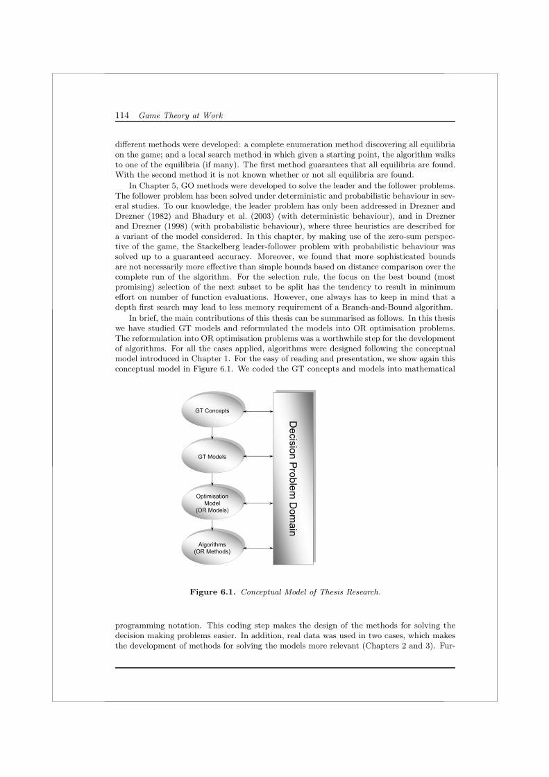
114 Game Theory at Work
different methods were developed: a complete enumeration method discovering all equilibriaon the game; and a local search method in which given a starting point, the algorithm walksto one of the equilibria (if many). The first method guarantees that all equilibria are found.With the second method it is not known whether or not all equilibria are found.
In Chapter 5, GO methods were developed to solve the leader and the follower problems.The follower problem has been solved under deterministic and probabilistic behaviour in sev-eral studies. To our knowledge, the leader problem has only been addressed in Drezner andDrezner (1982) and Bhadury et al. (2003) (with deterministic behaviour), and in Dreznerand Drezner (1998) (with probabilistic behaviour), where three heuristics are described fora variant of the model considered. In this chapter, by making use of the zero-sum perspec-tive of the game, the Stackelberg leader-follower problem with probabilistic behaviour wassolved up to a guaranteed accuracy. Moreover, we found that more sophisticated boundsare not necessarily more effective than simple bounds based on distance comparison over thecomplete run of the algorithm. For the selection rule, the focus on the best bound (mostpromising) selection of the next subset to be split has the tendency to result in minimumeffort on number of function evaluations. However, one always has to keep in mind that adepth first search may lead to less memory requirement of a Branch-and-Bound algorithm.
In brief, the main contributions of this thesis can be summarised as follows. In this thesiswe have studied GT models and reformulated the models into OR optimisation problems.The reformulation into OR optimisation problems was a worthwhile step for the developmentof algorithms. For all the cases applied, algorithms were designed following the conceptualmodel introduced in Chapter 1. For the easy of reading and presentation, we show again thisconceptual model in Figure 6.1. We coded the GT concepts and models into mathematical
OptimisationModel
(OR Models)
OptimisationModel
(OR Models)
OptimisationModel
(OR Models)
GT ConceptsGT ConceptsGT Concepts
Algorithms (OR Methods)
Algorithms(OR Methods) Algorithms
(OR Methods)
GT ModelsGT ModelsGT Models
Decision P
roblem D
omain
Decision P
roblem D
omain
Decision P
roblem D
omain
Figure 6.1. Conceptual Model of Thesis Research.
programming notation. This coding step makes the design of the methods for solving thedecision making problems easier. In addition, real data was used in two cases, which makesthe development of methods for solving the models more relevant (Chapters 2 and 3). Fur-

General Discussion and Conclusions 115
thermore, in one case we extended the GT model incorporating new ingredients (Chapter4). In another case, we have solved the model using GO techniques (Chapter 5).
6.4.2 Limitations of the Research and Suggestions for Further Research
In the scientific world, every study has its limitations and findings must be considered withinboundaries. However, looking at the optimistic part of limitations, boundaries are the nextstep on research. Of course, this research also had limitations and boundaries. Main rec-ommendation is that other cases could be studied in which other GT concepts, models, ORmodels and OR algorithms are applied. This study should be seen as a first step in makingGT more applicable to larger, more complex decision problems. The cases applied have spe-cific characteristics which guided us in the selection of specific GT models, OR models andalgorithms. First of all, Tables 1.1, 1.2 and 1.3 (Chapter 1) show the GT concepts/modelsand OR models/algorithms illustrated in this thesis. These are the first boundaries of theresearch. In the outline given, within decision making problems, less attention is given tobounded rationality. Further research can be directed to consider bounded rationality in deci-sion making problems. With respect to GT, we did not study incomplete information games.Research on cases with large number of players on incomplete information games are of in-terest. Further research could be done on the development of GT models, on the coding ofthese GT models into OR models and on the development of new OR methods/algorithms.It will contribute to further insight on GT concepts/models and OR models/techniques.When considering the OR models and algorithms used in this research, the models and algo-rithms developed in this study were based on the characteristic of the cases. Further researchincludes the study of the performance of the developed algorithms in comparison to otheralgorithms from OR. Next, limitations of the research are described by chapters.
In Chapter 2, further research could be done by studying a case in which multiple devia-tion is considered. In this chapter, stability is checked when only one player can deviate fromher strategy. If we consider multiple deviation, more than one player can deviate from theirstrategies. It will lead to more insights on GT as well as on OR formulation of models andalgorithms. Another limitation of the study is related to the algorithms. The developmentof new algorithms for this specific case could improve the performance of the enumerationmethod. If multiple deviation is considered, future research could study either to update thealgorithm developed or to develop new algorithms.
With respect to Chapter 3, one of the main limitations is the flexibility of the players(parties). To remain, the flexibility of a party (player) was defined by the radii of the maneu-vering space of the party, which consists of all acceptable positions. The maneuvering spacesare defined as a m-multidimensional Euclidean policy space. The flexibility of the playerswas selected for testing the formulated hypotheses. More research and theory developmentcould be done in order to derive a good setting for the flexibility of players in political games.A further step in selecting the flexibility data for the parties would make the output morerealistic. It is also interesting for further research to study the application of existing or newstability concepts of hedonic games.
Chapter 4 considers a game on location and quantity in a discrete location model. Themethods and cases consider the location on a node of a network. More research could bedone by considering that location is also possible at the edges. The question is if the multi-actor heterogeneous, free-entry and simultaneous location-quantity game can be reformulatedand coded. Challenge is the development of new algorithms for the characteristics of thegame. Moreover, the enumeration algorithm guarantees to find all the equilibria of the game,as in Chapter 1. Future research could also investigate the development of more efficient

116 Game Theory at Work
algorithms with the guarantee of finding all the equilibria.In Chapter 5, the quality (or size) of the facilities were assumed to be input data for
the model. An interesting way of further research is the development of new GO methodswhen considering the quality as another variable to be optimised. Within the settings ofthe problem of this research, it has been proven that more sophisticated bounds are notmore efficient. The question is if this still holds when applying the algorithms with otherways of branching. Another interesting way of looking at the problem is related to thebounding. Further research could focus on the development of more efficient bounds. WithinStackelberg (leader-follower) facility location games, another challenge for further research isto investigate new GO methods when more than two chains are competing (leader-followers).

BIBLIOGRAPHY
Altamirano-Cabrera, J. C. and Finus, M.: 2006, Permit trading and stability of internationalclimate agreements, Journal of Applied Economics IX (1), 19–48.
Altamirano-Cabrera, J., Finus, M. and Dellink, R.: 2005, Do abatement quotas lead to moresuccessful climate coalitions, Technical report, Working Paper in Economics 383. (HagenUniversity).
Arnold, T. and Schwalbe, U.: 2002, Dynamic coalition formation and the core, Journal ofEconomic Behaviour and Organization 40, 363–380.
Austen-Smith, D. and Banks, J.: 1988, Elections, coalitions and legislative outcomes, TheAmerican Political Science Review 82, 405–422.
Axelrod, R.: 1970, Conflict of interest, a theory of divergent goals with applications to politics,Chicago: Marham.
Baron, D.: 1993, Government formation and endogenous parties, The American PoliticalScience Review 87(1), 34–47.
Benders, J., Beulens, A. and van Nunen, J.: 1983, Groot Vademecum voor Bezuiniging en Be-sparing, De Toorts-Haarlem/Van der Wolk Publicaties-Laren NH
”chapter Operations
Research optimaliseert activiteiten, pp. 5.01–5.18.
Berge, C.: 1968, Principes de combinatoire.
Bhadury, J., Eiselt, H. and Jamarillo, J.: 2003, An alternating heuristic for medianoid andcentroid problems in the plane, Computers and Operations Research 30, 553–565.
Bloch, F.: 1995, Endogenous structures of association in oligopolies, Rand J. Econ. 26, 537–556.
Bloch, F.: 1996, Sequential formation of coalitions in games with externalities and fixedpayoff division, Games and Economic Behavior 14(1), 90–123.
Boggs, P. T. and Tolle, J. W.: 1996, Sequential quadratic programming, Acta Numerica4, 1–51.
Bosello, F., Carraro, C. and Buchner, B.: 2003, Equity, development, and climate changecontrol, Journal of the European Economic Association 1(2-3), 601–611(11).
Botteon, M. and Carraro, C.: 1997, International Environmental Negotiations: StrategicPolicy Issues, E. Elgar: Cheltenham, chapter Burden-Sharing and Coalition Stabilityin Environmental Negotiations with Asymmetric Countries, pp. ch. 3:26–55.
117

118 Game Theory at Work
Brams, S., Jones, M. and Kilgour, M.: 2005, Forming stable coalitions: The process matters.,Public Choice 125(1-2), 67–94.
Budge, I.: 1994, A new spatial theory of party competition: Uncertainty, ideology and policyequilibria viewed comparatively and temporally, British Journal of Political Science24(4), 443–467.
Bulow, J. I., Geanakoplos, J. D. and Klemperer, P. D.: 1985, Multimarket oligopoly: Strate-gic substitutes and complements, Journal of Political Economy 93(3), 488–511.
Carraro, C.: 1999, International Environmental Agreements on Climate Change, KluwerAcademic Publishers, Dordrecht, chapter The Structure of International Agreementson Climate Change.
Carraro, C., Bosello, F., Buchner, B. and Raggi, D.: 2001, Can equity enhance efficiency?lessons from the kyoto protocol, Technical report, FEEM Working Paper No. 49.2001.
Carraro, C. and Marchiori, C.: 2003, The Endogenous Formation of Economic Coalitions,E. Elgar: Cheltenham, chapter Stable Coalitions.
Casado, L. G., Hendrix, E. M. T. and Garcıa, I.: 2007, Infeasibility spheres for findingrobust solutions of blending problems with quadratic constraints, Journal of GlobalOptimization, doi: 10.1007/s10898-007-9157-x .
Colson, B., Marcotte, P. and Savard, G.: 2005, Bilevel programming: A survey, A QuarterlyJournal of Operations Research 3 (2), 87–107.
Cournot, A.: 1838, Recherches sur les Principes Mathematiques de la Theorie des Richesses(Englishedition, Researches into the Mathematical Principles of the Theory of Wealth,N.Bacon (ed.), 1897), Macmillan, New York.
Dantzig, G.: 1963, Linear Programming and Extensions, Princeton University Press, Prince-ton, New Jersey.
d’Aspremont, C., Jacquemin, A., Gabszewicz, J. J. and Weymark, J. A.: 1983, On thestability of collusive price leadership, Canadian Journal of Economics 16(1), 17–25.
de Ridder, A. and Rusinowska, A.: 2005, Different sequences of alliance formation, Technicalreport, Working paper series on Research in Relationship Management. RRM-2005-13-STR, Radboud University Nijmegen.
de Ridder, A., Rusinowska, A., Saiz, M. E. and Hendrix, E. M. T.: 2007, Coalition formation:the role of procedure and policy flexibility, Submitted .
Dellink, R. B., Altamirano-Cabrera, J. C., Finus, M., Ekko C. van Ierland, A. R. andWeikard, H. P.: 2003, Empirical background paper of the staco model, Technical report,mimeo, Wageningen University.
Dorta-Gonzalez, P., Santos-Penate, D. R. and Suarez-Vega, R.: 2004, Cournot oligopolisticcompetition in spatially separated markets: The stackelberg equilibrium, Ann. Reg. Sci.38 (3), 499 – 511.
Downs, A.: 1957, An economic theory of democracy, New York: Harper and Row Publishers.
Drezner, T.: 1994, Locating a single new facility among existing unequally attractive facili-ties., Journal Regional Science 34(2), 237–252.
Drezner, T. and Drezner, Z.: 1982, Competitive location strategies for two facilities, RegionalScience and Urban Economics 12, 485–493.
Drezner, T. and Drezner, Z.: 1994, Optimal continuous location of a retail facility, facilityattractiveness and market share: an interactive model, Journal of Retailing 70, 49–64.

Bibliography 119
Drezner, T. and Drezner, Z.: 1997, Replacing continuous demand with discrete demand ina competitive location model, Naval Research Logistics 44, 81–95.
Drezner, T. and Drezner, Z.: 1998, Facility location in anticipation of future competition,Location Science 6, 155–173.
Drezner, T. and Drezner, Z.: 2004, Finding the optimal solution to the huff based competitivelocation model, Computational Management Science 1, 193–208.
Drezner, Z. and Hamacher, H. W.: 2004, Facility Location: Applications and Theory,Springer Verlag.
Eiselt, H. and Laporte, G.: 1996, Sequential location problems, European Journal of Opera-tional Research 96, 217–231.
Eiselt, H., Laporte, G. and Thisse, J.-F.: 1993, Competitive location models: a frameworkand bibliography, Transportation Science 27, 44–54.
Enelow, J. and Hinich, M.: 1984, The spatial theory of voting. An introduction, Cambridge:Cambridge University Press.
Eyckmans, J. and Finus, M.: 2003a, Coalition formation in a global warming game: Howthe design of protocols affects the success of environmental treaty-making, Technicalreport, CLIMNEG WP 56.
Eyckmans, J. and Finus, M.: 2003b, New roads to international environmental agreements:The case of global warming, Technical report, FEEM Working Paper No. 88.2003.
Farrell, J. and Shapiro, C.: 1990, Horizontal mergers: An equilibrium analysis, Amer.Econom. Rev. 80(1), 107–26.
Fernandez, J., Pelegrın, B., Plastria, F. and Toth, B.: 2007, Solving a huff-like competitivelocation and design model for profit maximization in the plane, European Journal ofOperational Research 179, 1274–1287.
Finus, M., Altamirano-Cabrera, J. C. and van Ierland, E. C.: 2005, The effect of membershiprules and voting schemes on the success of international climate agreements, PublicChoice 125, 97–127.
Finus, M., Saiz, M. E. and Hendrix, E. M.: 2004b, An empirical test of new develpments incoalition theory for the design of international environmental agreements, Technical re-port, Mansholt Working Paper (Wageningen Universiteit). submitted to Environmental& Resource Economics.
Finus, M., van Ierland, E. and Dellink, R.: 2006, Stability of climate coalitions in a cartelformation game, Economics of Governance 7, 271–291.
Gomory, R. E.: 1958, Outline of an algorithm for integer solutions to linear programs,Bulletin of the American Mathematical Society 64, 275–278.
Grofman, B.: 1982, A dynamic model of protocoalition formation in ideological n-space,Behavioral Science 27(1), 77–90.
Hakimi, S.: 1983, On locating new facilities in a competitive environment, European Journalof Operational Research 12, 29–35.
Hendrix, E. M. T.: 2007, On the goodness of global optimisation algorithms, an introductioninto investigating algorithms, in A. Torn and J.Zilinskas (eds), Models and Algorithmsfor Global Optimization, Springer, New York, pp. 225–248.
Hillier, F. S. and Lieberman, G. J.: 1986, Introduction to Operations Research, McGraw-HillScience.

120 Game Theory at Work
Hotelling, H.: 1929, Stability on competition, The Economic Journal 39, 41–57.
Ibaraki, T.: 1976, Theoretical comparisons of search strategies in branch and bound algo-rithms, Int. J. Comput. Inform. Sci. 5, 315–344.
Karmarkar, N.: 1984, A new polynomial time algorithm for linear programming, Combina-torica 4, 373–395.
Keen, P. and Scott-Morton, M.: 1978, Decision Support Systems, an Organisational Per-spective, Addison Westley.
Klingemann, H.-D., Volkens, A., Bara, J. and Budge, I. (eds): 2006, Mapping Policy Pref-erences II: Estimates for Parties, Electors and Governments in Central and EasternEurope, European Union and OECD 1990-2003, Oxford: Oxford University Press.
Labbe, M. and Hakimi, S. L.: 1991, Market and locational equilibrium for two competitors,Operations Research 39(5).
Laver, M.: 2005, Policy and the dynamics of political competition, American Political ScienceReview 99(2), 263–281.
Laver, M. and Schofield, N.: 1990, Multiparty government: The politics of coalition in Europe,Oxford: Oxford University Press.
Laver, M. and Shepsle, K.: 1996, Coalitions and cabinet government, American PoliticalScience Review 84(3), 873–890.
Lederer, P. and Thisse, J.: 1990, Competitive location on networks under delivered pricing,Operations Research Letters 9, 140–153.
Martin, L. and Stevenson, R.: 2001, Government formation in parliamentary democracies,American Journal of Political Science 45(1), 33–50.
Martin, L. and Vanberg, G.: 2004, Policing the bargain: coalition government and parlia-mentary scrutiny, American Journal of Political Science 48(1), 13–27.
Mitten, L. G.: 1970, Branch and bound methods: general formulation and properties, Op-erations Research 18, 24–34.
Morasch, K.: 2000, Strategic alliances as stackelberg cartels - concept and equilibrium al-liance structure., International Journal of Industrial Organization 18(2), 257–282.
Muller, W. and Strøm, K.: 2003, Coalition governments in Western Europe, Oxford: OxfordUniversity Press.
Myerson, R.: 1991, Game Theory: Analysis of Conflict, Harvard University Press, Cam-bridge.
Nash, J.: 1951, Non-cooperative games, Annals of Mathematics 54, 298–95.
Nickel, S. and Puerto, J.: 2005, Location Theory. A Unified Approach, Springer.
Nordhaus, W. D.: 1994, Managing the Global Commons, Ed. MIT Press, Cambridge, MA.
Olieman, N. J. and Hendrix, E. M.: 2005, Stability likelihood of coalitions in a two-stagecartel game: An estimation method, forthcoming in European Journal of OperationalResearch .
Plastria, F.: 1992, Gbsss, the generalized big square small square method for planar singlefacility location, European Journal of Operational Research 62, 163–74.
Plastria, F.: 1997, Profit maximising single competitive facility location in the plane, Studiesin Locational Analysis 11, 115–126.

Bibliography 121
Plastria, F.: 2001, Static competitive facility location: an overview of optimisation ap-proaches, European Journal of Operational Research 129, 461–470.
Plastria, F. and Carrizosa, E.: 2004, Optimal location and design of a competitive facility,Mathematical Programming 100, 247–265.
Ray, D. and Vohra, R.: 1997, Equilibrium binding agreements, Journal of Economic Theory73, 30–78.
Ray, D. and Vohra, R.: 1999, A theory of endogenous coalition structures, Games andEconomic Behavior 26, 286–336.
Rhim, H., Ho, T. H. and Karmarkar, U. S.: 2003, Competitive location, production, andmarket selection, European Journal of Operational Research 149 (1), 211–228.
Riker, W.: 1962, The theory of political coalitions, Yale University Press.
Sarkar, J., Gupta, B. and Pal, D.: 1997, Location equilibrium for cournot oligopoly inspatially separated markets, Journal of Regional Science 37 (2), 195–212.
Schrijver, A.: 1998, Theory of Linear and Integer Programming, John Wiley & Sons, NewYork.
Selten, R.: 1975, Reexamination of the perfectness concept for equilibrium points in exten-sivegames, International Journal of Game Theory 4, 25–55.
Shubik, M.: 1984, Game Theory in the Social Sciences: Concepts and Solutions, MIT Press.Cambridge, MA.
Simon, H.: 1976, Administrative behaviour, a study of decision making processes in admin-istrative organisations, New York/London.
Simon, H. A., Dantzig, G. B., Hogarth, R., Piott, C. R., Raiffa, H., Schelling, T. C., Shepsle,K. A., Thaier, R., Tversky, A. and Winter, S.: 1986, Research Briefings 1986, NationalAcademy Press, Washington, DC., chapter Report of the Research Briefing Panel onDecision Making and Problem Solving, pp. 17–36.
Saiz, M. E., Hendrix, E. M. T. and Olieman, N. J.: 2006, On the computation of stabilityin multiple coalition formation games, Computational Economics 28 (3), 251–275.
Saiz, M. E., Olieman, N. J., Hendrix, E. M. and Finus, M.: 2004, Determination of stablestructures in a multiple coalition game, Technical report, Mansholt Working Paper(Wageningen Universiteit).
Stackelberg, H. V.: 1934, Marktform und Gleichgewicht, Vienna: Julius Springer.
Teitz, M. and Bart, P.: 1968, Heuristic methods for estimating the generalized vertex medianof a weighted graph, Operations Research 16, 955–961.
Thoron, S.: 2000, Interaction and Market Structure, Springer Verlag, chapter Market orga-nization: Noncooperative models of coalition formation, pp. 207 – 223.
Timmermans, A.: 2003, High politics in the low countries. An empirical study of coalitionagreements in Belgium and The Netherlands, Aldershot: Ashgate.
Tohme, F. and Sandholm, T.: 1999, Coalition formation processes with relief revision amongbounded rational self-interested agents, Journal of Logic and Computation 9, 793–816.
Tuy, H., Al-Khayyal, F. and Zhou, F.: 1995, A d.c. optimization method for single facilitylocation problems, Journal of Global Optimization 7, 209–227.
van Deemen, A.: 1989, Dominant players and minimum size coalitions, European Journal ofPolitical Research 17, 313–332.

122 Game Theory at Work
van Deemen, A.: 1997, Coalition formation and social choice, Boston: Kluwer AcademicPublisher.
van der Brug, W.: 1999, Voters’ perceptions and party dynamics, Party Politics 5(2), 147–169.
van der Vorst, J. G.: 2000, Effective Food Supply Chains; generating, modelling and evalu-ating supply chain scenarios, PhD thesis, Wageningen Universiteit.
Volden, C. and Carrubba, C.: 2004, The formation of oversized coalitions in parliamentarydemocracies, American Journal of Political Science 48(3), 521–537.
von Neumann, J. and Morgenstern, O.: 1944, Theory of Games and Economic Behavior,Princeton: Princeton University Press.
Vries, M. D.: 1999, Governing with your closest neighbour: An assessment of spatial coalitionformation theories, Enschede: Print Partners Ipskamp.
Warwick, P.: 1998, Policy distance and parliamentary government, Legislative Studies Quar-terly 23(3), 319–345.
Warwick, P.: 2000, Policy horizons in west european parliamentary systems, European Jour-nal of Political Research 38, 37–61.
Warwick, P.: 2005a, When far apart becomes too far apart: Evidence for a threshold effectin coalition formation, British Journal of Political Science 35, 383–401.
Warwick, P.: 2005b, Do policy horizons structure the formation of parliamentary govern-ments?: The evidence from an expert survey, American Journal of Political Science49(2), 373–387.
Weikard, H., Finus, M. and Altamirano-Cabrera, J.: 2006, The impact of surplus sharing onthe stability of international climate agreements, Oxford Economic Papers 58, 209–232.
Yi, S.-S.: 1997, Stable coalition structures with externalities, Games and Economic Behavior20, 201–237.
Yi, S.-S. and Shin, H.: 1995, Endogenous formation of coalitions in oligopoly, DartmouthCollege Department of Economics WP No. 95-2, 537–556.

SummaryDecision making is present in daily life. A decision making problem appears when there is aneed to take a decision. Most of the decisions have a goal; a set of variables, characteristicsdefining a problem, that need to be optimised. A decision problem can be formulated andmodelled using Game Theory (GT) and Operations Research (OR) methods. Based on themodel, solution alternatives are generated and evaluated in order to obtain a preference orderof the alternatives based on the objective of the decision maker. Decision situations may alsoinvolve multiple decision makers, leading to cooperative and/or competitive decision makingsituations.
GT may have modelling merits to contribute to decision making situations where decisionmakers have competing or cooperating objectives, under the assumption that the decisionmakers are rational and they act in their best own interest. GT models are often appliedto situations with few or symmetric multiple decision makers, which limits its modellingpower. Results in existing literature are often attributable to basic models with only twoactors leading to analytical solutions or alternatively to more actors that are all assumed tobe the same; symmetric players. In this thesis we contribute to cooperative or competitivedecision situations by building new or existing GT models and by reformulating those intoOR models to study cases with more than two heterogeneous actors. To solve those decisionmaking problems, one has to apply and develop new OR techniques by developing models andalgorithms. Looking at relevant literature, decision situations like environmental decisions,supply chains decisions and political games are of interest for research.
The research objective of this thesis is to develop or contribute to the development ofusable GT models and OR methods to solve decision making problems in practical situations.We modelled those problems with new or existing GT models for multiple, asymmetric andheterogeneous actors in cooperative/non-cooperative and competitive decision situations.The GT models are reformulated using OR techniques and new OR algorithms are developedfor obtaining the optimal solutions for the models.
We hypothesised that GT concepts and models might provide us with a valuable contri-bution for supporting decision makers provided that we can make OR models and algorithmsto solve these models. In order to achieve the objective of this thesis four research questionsare addressed:
1. How do we formulate GT models for decision making situations with multiple hetero-geneous actors using GT concepts? How can we contribute to that modelling?
2. If we have GT based models: What appropriate coding can be used to translate aspecific GT model into a mathematical programming optimisation problem such thatit can be solved?
3. Which solution methods can be developed to solve these models?

124 Game Theory at Work
4. How do the outcomes aid to analyse the decision makers problem? or What is thecontribution of the new outcomes to the decision makers problem?
In answering the research questions, four different cases are used. In all the cases, new orexisting GT models are developed and reformulated into OR optimisation models and ORalgorithms for solving these models. The starting points for each of the cases are from sourcesbased on literature review. To illustrate cooperative/non-cooperative GT concepts/modelswe looked for models with a challenge on algorithmic development. Two types of coalitionformation are considered: multiple coalition formation and single (cartel) coalition formation(Chapter 2 and Chapter 3). To illustrate competition models, we looked for cases involvingcompetition on location and competition on location and quantity (Chapter 4 and Chapter5). The objective is to contribute to these models extending the research either on the GTmodels and reformulation to OR models or the OR methods.
Chapter 2 describes a multiple coalition formation game in which membership rules anddifferent transfer schemes are described. Open membership rule is used to indicate thatfor the current members of a coalition, any other player is allowed to enter it. Exclusivemembership rule implies that a non-member is only allowed to join the existing coalitionif the payoff (outcome) for the existing coalition members will not decrease, only in thatcase the members of the existing coalition will allow the new member to join them. Ifnot, they will exclude her. The study also considers two types of voting rules: MajorityVoting, where the majority of the members of the coalition have the decision on yes/no tothe new coalition potential partner and Unanimity Voting, when one coalition member candisapprove when a new member wants to join. Moreover, four different transfer schemesare used, namely: “Equal Sharing”, “Population”, “Gross Domestic Product” and “Ability toPay”. Given the GT model and the OR model, the goal is to develop methods for checkingstability of coalition structures. For the check of stability we need all the neighbours of eachcoalition structure. Neighbours in a coalition structure for each player are determined bythe single deviation from players to other coalitions or players deviating and being alone,that means becoming a singleton player. The exact number of neighbours is not easy toidentify. The larger the number of players is, the larger the number of coalition structuresand as a consequence, the bigger the matrix with all necessary data to test stable coalitionstructures. A new mathematical programming formulation, crucial for the development ofthe algorithms, is elaborated. Available data is used to determine which stable coalitionsappear and which procedures can be used to make coalitions stable. A case study on theKyoto negotiation process is applied to check the algorithms. Main conclusions are thattransfer schemes are useful to be implemented and computation with membership rulesgenerate different results with and without transfer schemes. In the cases without transfers,the algorithm only found stability when an exclusive membership game with unanimityvoting rule is applied. This result is different when transfers are applied; either majorityand unanimity voting are sufficient to stabilise coalition structures. With respect to thenumber of stable coalition structures, there are some transfer schemes which do not generatestable coalition structures. Transfer schemes are anyway interesting in terms of net benefitand global emission reduction. Furthermore, some of the regions considered that are “notinterested” in cooperation without transfer schemes, became interested in forming a coalitionwhen transfers appear. Furthermore, the resulting model was used in further studies (Finuset al. (2006), Altamirano-Cabrera and Finus (2006), Finus et al. (2005), Weikard et al. (2006)and Altamirano-Cabrera et al. (2005)).
Chapter 3 studies a model of multidimensional coalition formation in politics. Thereare n parties trying to form a government. A formed government has a policy agreementrepresented in a m-multidimensional Euclidean policy space R
m. The complexity increaseswith the number of parties n and the dimension of the policy spaces m. Given the number

Summary 125
of parties n and policy dimension m, computational methods are necessary to compute allpossible winning coalitions and preferences of parties over those coalitions. Furthermore, twoways of forming a government are considered: step-by-step and simultaneously. Proceduresdiffer from each other, but they have in common that no party will agree on a position whichdoes not belong to its maneuvering space as these positions are unacceptable for a party.In other words, the position of the formed coalition must belong to the intersection of themaneuvering spaces of the potential coalition. Calculations show that the number of differentpaths and coalition positions in the step-by-step procedure can increase dramatically. Forcomputing the output of the model, computational methods are necessary and algorithms forthe different procedures are introduced. The algorithms determine the compromise (coalitionposition) points of all winning coalitions as well as preference order based on distances toideal points. The developed algorithms use an external procedure for the determination of theoutput based on sequential quadratic programming (SQP) methods. Moreover, a penaltyapproach is developed to determine whether or not feasible negotiation spaces intersectbetween the negotiating parties (the players of the game). The analysis in de Ridder et al.(2007) focused on three aspects of coalition formation and formulated hypotheses: procedure,flexibility, and power sharing. By applying the developed algorithms to Dutch data andtheoretical examples, several hypotheses are tested and implications for political partiesinvolved in coalition formation are given.
Chapter 4 describes a competitive two-stage location-quantity game with m > 2 marketsand n > 2 firms. In the first stage of the game location decisions by firms are taken; in thesecond stage, firms decide about quantities to supply at each of the markets. At each step,decisions are simultaneous. The location space is discrete, in particular is a network wherethe nodes are considered as the possible locations. Free entry is possible, the number offirms entering the markets is not known in advance; and costs are asymmetric, firm-specific.Analytical solutions for the supplying decisions and properties for determining the size of themarket are derived. The computation of the optimum quantities to supply (equilibrium) ispossible when market sizes are determined. In finding the equilibria on location, a completeenumeration algorithm and a local search algorithm are used. The complete enumerationalgorithm guarantees that all the equilibria of the game are found. The local search algorithmaims at finding one equilibrium given a starting point. Two cases are elaborated to illustratethe procedures and the analytical results. The first case is taken from literature with n = 3firms and m = 6 markets. The second numerical example consists of 4 different cases. It isused to show the viability of the algorithms when bigger and more sophisticated cases areapplied. Furthermore, by using the algorithms as a systematic computation instrument tocases reported in literature, a mistake is detected in Sarkar et al. (1997). In that paper asolution is given that appears not to be an equilibrium of the model.
Chapter 5 deals with a competitive facility location problem in which the concept ofStackelberg leader-follower problem is applied. There is a leader chain who wants to locatea facility and a follower chain taking the location decision after the leader. The marketshare captured by a firm is given by a gravity model determined by distance calculations tofacilities. The follower problem, is known to be a hard global optimisation problem. Theleader problem is even harder, since the leader has to decide on location given the optimalaction of the follower. So far, in literature only heuristic approaches have been tested to solvethe leader problem. Branch-and-Bound (B&B) algorithms for the leader and the followerare designed. The B&B algorithm for the leader has to solve two follower problems: one forsolving (and anticipating) the optimal location of the follower (already a GO problem) andthe second one for obtaining an upper bound for her own B&B algorithm (GO problem). Forthe B&B algorithm for the follower problem, four different upper bounds are derived. Thealgorithm evaluates and chooses the best of the four upper bounds. The branching rule uses

126 Game Theory at Work
rectangles and new rectangles are generated by bisecting a rectangle over its longest edge.Moreover, two variants are implemented and compared: starting with an initial rectanglecontaining the feasible area, and starting with an initial partition into rectangles. It isoutlined that, although generating an initial partition improves the upper bounding applied,it generates more partition sets than strictly necessary. Furthermore, two selection rulesare compared: breadth-first-search and best-bound-search. The effect on efficiency of thoserules is measured. The effectiveness and efficiency of the algorithms are investigated withthe aid of numerical cases. As main conclusion, it is found that more sophisticated boundsare not necessarily more effective than simple bounds based on distance comparison over thecomplete run of the algorithm. One can best focus on measuring the quality of the boundduring the run and take the sharpest one. For the selection rule, the focus on the bestbound (most promising) selection of the next subset to be split has the tendency to resultin minimum effort on number of function evaluations. As memory requirement is usually aproblem for higher dimensions, it is not necessarily a focus point for the location problem intwo dimensional space.
By answering the research questions, the main conclusions of this study are outlined.Within the research of this study, GT has been a useful tool for modelling decision mak-ing situations when multiple, asymmetric and heterogeneous decision makers are involved.Contribution to GT models is most significant in Chapter 2 and Chapter 4 by adding ad-ditional characteristics to cases taken from literature. An important factor in this thesis iswhat is called “coding into mathematical programming notation”; it has a relevant contri-bution on the development of algorithms to solve the decision making problems. From thecases studied, different challenges inspired the development of the algorithms: applicationto huge cases, asymmetry, heterogeneity and multiple actors. Algorithms are developed foreach of the problems covered in this research; algorithms are based on enumeration methods,iterative approaches, analytical solutions, SQP methods, penalty approach and GO methods.
In brief, the main contributions of this thesis can be summarised as follows. In this thesiswe have studied GT models and reformulated the models into OR optimisation problems.The reformulation into OR optimisation problems is a worthwhile step for the developmentof algorithms. Furthermore, in this research, both real-life data and randomly generateddata are used. For all the cases applied, algorithms are designed following the conceptualmodel introduced in Chapter 1. The idea is that outcomes of the developed algorithms aimto help decision makers and analysts to get insight into a decision situation. Two of thecases contributed on aiding researches when real data are used (Chapters 2 and 3). Modelsand methods in Chapters 4 and 5 are illustrated with randomly generated data.
This study should be seen as a first step in making GT more applicable to larger, morecomplex decision problems. The cases applied have specific characteristics which guided usin the selection of specific GT models, OR models and algorithms. Within decision makingproblems, we have focused on rational behaviour of decision makers. Further research couldbe done by considering bounded rationality in decision making problems. With respectto GT, incomplete information games have not been studied. It is of interest to do moreresearch on cases with large number of players on incomplete information games and howto contribute on the development of GT models, on the coding of these GT models into ORmodels and on the development of new OR methods/algorithms. When considering the ORmodels and algorithms, the models and algorithms developed in this study are focused onthe characteristic of the cases. Further research includes the study of the performance ofthe developed algorithms in comparison to other algorithms from OR. In summary, thereexist new challenges on developing Operations Research models and algorithms to get GameTheory at work.

SamenvattingHet nemen van beslissingen is een dagelijkse bezigheid. Vaak is er sprake van een te op-timaliseren doelstelling en diverse variabelen die het probleem karakteriseren. Een besliss-ingsprobleem kan worden geformuleerd en gemodelleerd met behulp van speltheorie en Op-erations Research methoden. Beslissingsalternatieven worden gegenereerd en geevalueerd,zodat een preferentievolgorde van de alternatieven ontstaat, gebaseerd op de doelstelling vande besluitvormer. Beslissingsituaties kunnen ook meerdere beslissers bevatten die samen-werking of competitie nastreven.
Speltheorie heeft de potentie om bij te dragen aan beslissingssituaties waarbij de be-langhebbenden samenvallende of conflicterende doelstellingen hebben, zolang wordt aan-genomen dat de besluitvormers rationeel handelen voor hun eigen bestwil. Gewoonlijkwordt speltheorie toegepast om situaties te beschrijven met een beperkt aantal identiekebesluitvormers. Dit beperkt de kracht van de analyse. In de bestaande literatuur zien wevaak basale modellen met slechts twee actoren, zodat analytische oplossingen kunnen wordeafgeleid. Als alternatief zien we situaties met meerder identieke actoren beschreven. Ditproefschrift draagt bij aan de modellering van samenwerkende en conflicterende beslissingsi-tuaties door het bouwen van bestaande of nieuwe speltheoretische modellen en door hetomzetten daarvan naar OR modellen om cases met meer dan twee heterogene actoren tebestuderen. Om deze problemen op te lossen worden nieuwe OR technieken ontwikkelddoor het uitwerken van modellen en algoritmen. Gebaseerd op de literatuur, zijn besliss-ingsituaties met milieubeslissingen, met betrekking to ”supply chainsen in politieke situatiesinteressant.
De doelstelling van dit proefschrift is om bij te dragen aan de ontwikkeling van bruik-bare speltheoretische modellen en OR methoden om praktische beslissingssituaties op telossen. Daartoe werden nieuwe en bestaande speltheoretische modellen ontwikkeld voor hetbeschrijven van beslissingssituaties met asymmetrische, heterogene actoren die wel of nietsamenwerken en conflicterende doelstellingen hebben. De modellen zijn omgezet met behulpvan OR methoden en nieuwe algoritmen zijn ontwikkeld om optimale resultaten voor demodellen af te leiden. De hypothese is dat speltheoretische concepten en modellen zoudenkunnen bijdragen aan het ondersteunen van besluitvormers indien we in staat zijn om ORmodellen en algoritmen te maken die bijdragen aan de oplossing ervan. Om de doelstellingte bewerkstelligen worden vier onderzoeksvragen geformuleerd en uitgewerkt:
1. Hoe kunnen we speltheoretische modellen ontwikkelen voor beslissingsituaties metmeerdere heterogene actoren vanuit speltheoretische concepten? Hoe kunnen we bij-dragen aan de modellering?
2. Als we eenmaal modellen hebben gebaseerd op speltheorie, welke codering kan wordengebruikt om een speltheoretisch model om te zetten naar een wiskundig optimaliser-
128 Game Theory at Work
ingprobleem zodat het kan worden opgelost?
3. Welke technieken kunnen worden toegepast om dit soort problemen op te lossen?
4. Hoe dragen de uitkomsten bij aan het analyseren van het beslissingprobleem? Wat isde bijdrage van de nieuwe uitkomsten aan het begrijpen van het beslissingprobleem?
Voor het beantwoorden van de onderzoeksvragen worden vier cases uitgewerkt. In elkecase wordt een nieuw of bestaand speltheoretisch model uitgewerkt en omgezet naar eenOR optimaliseringprobleem. Algoritmen worden ontwikkeld om het probleem op te lossen.Elke case is gebaseerd op een literatuuronderzoek. Om cooperatieve versus non-cooperatievespeltheorie te illustreren zochten we naar modellen met een uitdaging op algoritmisch gebied.Twee typen coalitievorming zijn onderzocht: vorming van meervoudige coalities en vormingvan een enkelvoudige (kartel) coalitie (hoofdstukken 2 en 3). Voor de illustratie van com-petitieve modellen richtte de aandacht zich op concurrentie tussen aanbieders op het gebiedvan locatie en concurrentie met betrekking tot aangeboden hoeveelheid en locatie (hoofd-stukken 4 en 5). De doelstelling is om bij te dragen aan het onderzoek door de ontwikkelingvan speltheoretische modellen, de vertaling richting OR modellen en het bijdragen aan deoplossingmethode.
Hoofdstuk 2 beschrijft een spel van coalitievorming met verschillende lidmaatschapregelsen verschillende herverdelingregels. Een open lidmaatschap”betekent dat de huidige ledenhet goed vinden dat een andere actor lid wordt. Een exclusief lidmaatschap”regel betekentdat een aspirant lid alleen lid kan worden van de coalitie als het voordeel (baten) voor dehuidige leden er niet op achteruit gaat. Binnen dit kader bekijkt de studie twee stemproce-dures: meerderheid stemming, waarbij de meerderheid van de huidige leden beslist om eennieuw lid wel of niet toe te laten en unanimiteit, waarbij een lid voldoende is om lidmaatschapvan een aspirant lid te blokkeren door middel van een veto. Verder worden vier verschil-lende schema’s gebruikt om de baten te (her)verdelen, namelijk: ”gelijk delen”. ”bevolking”,”GDPen ”koopkracht”. Gegeven het speltheoretisch model en de vertaling daarvan naareen OR probleem, is de uitdaging om methoden te ontwikkelen die de stabiliteit van eencoalitie testen. Voor deze test is het nodig om van een coalitiestructuur alle aanpalende ofbuur-coalitiestructuren te kennen. Zo’n buur wordt bepaald doordat een van de spelers haarstrategie verandert; of een lid van een coalitie gaat naar een andere coalitie of gaat alleenverder; of een speler die nog geen lid is wordt lid van een coalitie. Het precieze aantal burenis niet eenvoudig te bepalen. Hoe meer spelers, hoe groter het aantal coalitiestructuren enhoe groter de matrix die alle nodige informatie bevat om stabiliteit te testen. Een nieuwemathematisch besliskundige formulering is uitgewerkt voor het ontwikkelen van algoritmen.Beschikbare gegevens zijn gebruikt om na te gaan welke coalitiestructuren stabiel zijn enwelke procedures de stabiliteit kunnen bevorderen. Een case over het Kyoto onderhandel-ingproces is gebruikt om algoritmen te testen. Belangrijkste conclusies zijn dat het nuttigkan zijn om herverdelingschema’s te implementeren en dat berekeningen met verschillendelidmaatschapregels verschillende resultaten geven voor verschillende herverdelingschema’s.In gevallen zonder herverdeling, vond het algoritme alleen stabiele coalities als een exclusieflidmaatschapregel bestaat met veto stemming. Als herverdeling wordt geıntroduceerd kun-nen coalities ook stabiel worden bij meerderheid stemming. Als wordt gekeken naar hetaantal stabiele coalities kan worden opgemerkt dat er herverdelingschema’s zijn die geenenkele stabiele coalitie geven. Herverdelingschema’s zijn altijd van belang als we kijken naarde totale baten en globale emissiereductie. Bovendien blijken sommige regio’s die zonderherverdeling niet geınteresseerd zijn in samenwerking wel geınteresseerd om tot een coali-tie toe te treden wanneer er wel herverdelingschema’s bestaan. De ontwikkelde methodiekis toegepast in verdere studies, zoals (Finus et al. (2006), Altamirano-Cabrera and Finus(2006), Finus et al. (2005), Weikard et al. (2006) and Altamirano-Cabrera et al. (2005).

Samenvatting 129
Hoofdstuk 3 beschrijft een model over meerdimensionale coalitievorming in de politiek.Er zijn n partijen die proberen te komen tot een coalitieregering. De gevormde regeringheeft een politieke agenda (overeenkomst) die gerepresenteerd wordt door een punt in eenm-meerdimensionale Euclidische politieke ruimte. De complexiteit van de analyse neemt toemet het aantal partijen n en de dimensie m van de politieke ruimte. Rekenmethoden zijnnodig om alle mogelijke meerderheidcoalities te bepalen en de preferenties van de partijen overde coalities. Twee mogelijke procedures voor het vormen van een coalitie worden bestudeerd:een stap-voor-stap procedure en een simultane procedure. Onafhankelijk van de procedure zaleen partij niet tot een overeenkomst komen als die niet ligt binnen haar spelingruimte. Metandere woorden, een overeenkomst van een gevormde coalitie moet liggen in de doorsnede vande spelingruimten van de partijen die behoren tot de coalitie. Berekeningen hebben laten ziendat het aantal mogelijke paden om tot coalities te komen en de bijbehorende overeenkomstendrastisch kan toenemen met het aantal partijen. Om de uitkomst van het model te bepalenzijn rekenmethoden nodig; algoritmen voor de verschillende procedures zijn uitgewerkt. Dealgoritmen bepalen de compromis overeenkomsten van alle meerderheidcoalities zowel alsde preferentie van de verschillende partijen gebaseerd op de afstand van de overeenkomsttot hun ideale politieke agenda. De ontwikkelde algoritmen gebruiken een externe routinegebaseerd op sequentiele kwadratische programmering (SQP). Verder is een boetefunctieaanpak uitgewerkt om te bepalen of de onderhandelende partijen wel onderhandelingruimtehebben bestaande uit de doorsnede van de spelingruimten. De analyse in de Ridder et al.(2007) concentreert zich op drie aspecten t.a.v. coalitievorming en test daar hypothesenover: de procedure, de flexibiliteit en het delen van macht. Door de ontwikkelde algoritmentoe te passen op gegevens uit de Nederlandse politiek en op theoretische voorbeelden zijn dehypothesen getest en consequenties voor partijen betrokken bij een onderhandeling wordengegeven.
Hoofdstuk 4 beschrijft een competitief spel bestaande uit twee fasen besluitvorming: lo-catie beslissing en hoeveelheid beslissing, waarin n>2 bedrijven concurreren op m>2 mark-ten. In de eerste fase van het spel nemen de bedrijven een beslissing t.a.v vestiging op eenlocatie. In de tweede fase besluiten ze de hoeveelheid die ze aanbieden op de markten. Inbeide fasen worden de beslissingen simultaan genomen. De vestigingruimte is discreet, waar-bij de potentiele locaties bestaan uit knopen in een netwerk. De bedrijven zijn vrij om eenmarkt te bevoorraden, zodat men niet van te voren weet hoeveel bedrijven een markt zullenbenaderen. De kosten zijn bedrijfafhankelijk, dus asymmetrisch. Voor het vinden van eenevenwicht t.a.v. de vestigingbeslissing zijn een aftelalgoritme en een lokale zoekprocedureontwikkeld. Het aftelalgoritme vindt alle mogelijke evenwichten. De lokale zoekprocedurevindt een evenwicht vanuit een startconfiguratie. Twee cases zijn uitgewerkt om de proce-dures en analytische resultaten te illustreren. De eerste case uit de literatuur beschrijft eeninstantie met n = 3 bedrijven en m = 6 markten. Het tweede numerieke voorbeeld bevat4 instanties met toenemende grootte. Het laat zien dat problemen van toenemende groottekunnen worden aangepakt met de ontwikkelde procedures. Gebruik van de algoritmen optestcases uit de literatuur leidde tot de ontdekking van een fout in Sarkar et al. (1997). Eengepresenteerde oplossing van een model in het artikel blijkt geen evenwicht te zijn.
Hoofdstuk 5 behandelt een competitief vestigingprobleem waarin het Stackelberg conceptvan de leider-volger wordt toegepast. Een leider winkelketen vestigt eerst een filiaal en eenvolgketen opent vervolgens een vestiging. Het marktaandeel dat een keten verovert wordtbeschreven door een zwaartepunt model gebaseerd op de afstanden tussen vestigingen enklanten. Het is bekend uit de literatuur dat het vinden van de beste locatie voor de volgketeneen moeilijk globaal optimaliseringprobleem (GO) is. Het probleem van de leider is echternog moeilijker, daar die rekening moet houden met de optimale locatie van de volger. Voorzover we weten werd het leiderprobleem in de literatuur alleen met heuristische methoden

130 Game Theory at Work
aangepakt. In dit proefschrift worden Branch-and-Bound (B&B) algoritmen voor het leider-en volgprobleem ontworpen. Het algoritme voor de leider vereist in elke iteratie dat tweevolgproblemen worden opgelost: een voor het bepalen van de optimale locatie voor de volgeren een voor het bepalen van een bovengrens voor de leider, beide GO problemen. Voorhet B&B algoritme voor het volgprobleem zijn vier verschillende bovengrenzen (bounds)ontworpen. Het algoritme berekent de waarden ervan in elke iteratie en gebruikt de strakstegrens. Het vertakken (branching) naar subproblemen werkt met rechthoeken die gesplitstworden over de langste zijde. Twee strategieen zijn uitgeprobeerd. Een waarbij de rechthoekvan het toegelaten gebied als startgebied wordt genomen en een waarbij deze rechthoek alis gepartitioneerd naar sub-rechthoeken. De studie laat zien dat hoewel de initiele partitiede waarden van de grenzen verbetert, het algoritme niet in efficientie wint, omdat teveelsub-rechthoeken worden geprobeerd. Twee keuzeregels zijn vergeleken voor de keuze van derechthoek die wordt bekeken: zoeken in de breedte en prioriteit voor de beste grens. Deefficientie is gemeten voor beide regels. Effectiviteit en efficiency is nagegaan met behulpvan numerieke instanties. Een belangrijke conclusie is dat verfijnde grenzen niet noodzakelijkbetere resultaten geven dan een eenvoudige grens die gebaseerd is op het onderschatten vanafstand tussen klant en filiaal. Het beste is om de scherpste grens te nemen gedurendehet verloop van het algoritme. Voor de keuzeregel van de volgende rechthoek die wordtgesplitst heeft focus op de beste grens de neiging om het minst aantal iteraties te vereisen.Gewoonlijk is voor dit soort algoritmen het geheugenbeslag een probleem wanneer toegepastin hogere dimensies. Voor het locatieprobleem is dit minder het geval omdat het zich in detweedimensionale ruimte afspeelt.
Voor de belangrijkste conclusies richten we ons op de onderzoeksvragen. De studielaat zien dat speltheorie een handig hulpmiddel kan zijn voor het modelleren van besliss-ingsituaties met meerdere asymmetrische en heterogene belanghebbenden. De bijdrage aanspeltheoretische modellen is belangrijk in hoofdstukken 2 en 4, waarbij nieuwe aspecten aanbestaande modellen zijn toegevoegd. Een belangrijke factor in dit proefschrift is wat genoemdwordt de ”codering van modellen in mathematische programmering taalı.e. het vertalen naarwiskundige optimaliseringproblemen. Dit is met name relevant voor het ontwikkelen vanalgoritmen om beslissingproblemen op te lossen. De bestudeerde cases bevatten diverse in-teressante aspecten voor de ontwikkeling van algoritmen: toepassing van grote instanties,asymmetrie, heterogeniteit en meerdere actoren. Algoritmen zijn ontwikkeld voor elk prob-leem dat in deze studie is aangepakt. De algoritmen zijn gebaseerd op volledige aftelling,iteratieve methoden, analytische oplossingen, SQP methoden, boetefunctie aanpakken englobale optimalisering.
De belangrijkste bijdragen van dit proefschrift kunnen als volgt worden samengevat.In dit proefschrift zijn diverse speltheoretische modellen bestudeerd en vertaald naar ORoptimaliseringmodellen. Het herformuleren van modellen naar optimaliseringproblemen iseen nuttige stap voor het ontwikkelen van algoritmen. Gegevens in dit onderzoek komen uitde praktijk of zijn random gegenereerd. Voor elke casus zijn algoritmen ontwikkeld volgenshet conceptuele model in hoofdstuk 1. Het doel van de uitkomsten van de algoritmen isdat ze de besluitvormers helpen om inzicht te krijgen in een beslissingsituatie. Twee caseshielpen onderzoekers voor het uitwerken van gegevens uit de praktijk (hoofdstukken 2 en3). De modellen en methoden in hoofdstukken 4 en 5 worden met name geıllustreerd doorrandom gegenereerde gegevens.
Deze studie kan gezien worden als een eerste stap om speltheorie toepasbaar te makenvoor grotere en complexere beslissingproblemen. De bestudeerde cases gaven aanleiding totselectie van specifieke speltheoretische modellen, OR modellen en algoritmen. Binnen detheorie van de beslissingproblemen hebben we ons gericht op het rationeel handelen vanactoren. Verder onderzoek kan worden gedaan op het gebied van begrensde rationaliteit

Samenvatting 131
in beslissingsituaties. Met betrekking tot speltheorie zijn modellen met onvolledige infor-matie niet bestudeerd. Het kan interessant zijn om onderzoek te doen naar gevallen meteen groot aantal spelers (actoren) die geen volledige informatie hebben en te bestuderen hoedit soort modellen gecodeerd kunnen worden in OR modellen die nieuwe typen OR algorit-men/methoden vereisen. De modellen en methoden die ontwikkeld zijn in dit proefschriftzijn toegespitst op de karakteristieken van de bestudeerde cases. Verder onderzoek bevatde bestudering van de prestatie van de ontwikkelde algoritmen in vergelijking tot anderealgoritmen uit de OR. Samengevat bestaan er verdere uitdagingen in de ontwikkeling vanOperations Research modellen en methoden om speltheorie aan het werk”te krijgen.

ResumenEl proceso de la toma de decisiones (teorıa de la decision) esta presente en la vida diaria.Inherente a la toma de decisiones es la necesidad de elegir entre diferentes alternativas. Lamayorıa de las decisiones tienen una meta u objetivo, y se toman en base a un conjunto devariables que definen un problema y que necesitan ser optimizadas. Los problemas de tomade decisiones pueden ser formulados y modelados usando la Teorıa de Juegos (TJ) y metodosde Investigacion Operativa (IO). En base al modelo, se generan soluciones alternativas queson evaluadas para obtener un orden de preferencia dependiendo del objetivo del agenteresponsable de tomar la decision (agente o jugador mas adelante). La toma de decisionespuede involucrar a mas de un agente, lo cual genera problemas cooperativos y/o competitivos.
Por lo tanto, la TJ es una herramienta muy valiosa a la hora de modelar problemas dedecisiones en los cuales los objetivos de los jugadores son de tipo cooperativo o competitivo,y donde los jugadores actuan de forma racional y en su propio interes. En ocasiones la TJes usada para modelar juegos en los que el numero de jugadores es reducido o los juegosson simetricos, lo que limita su potencial de modelado. En la literatura existente se puedenencontrar resultados en modelos basicos con solo 2 jugadores en los que se obtienen solucionesanalıticas, y/o modelos con mas jugadores asumiendo simetrıa. Esta tesis contribuye a laTJ mediante la construccion de nuevos modelos o el uso de los ya existentes con mas de dosjugadores heterogeneos y mediante la construccion o reformulacion en modelos de IO. Paraobtener una solucion a dichos modelos es necesaria la aplicacion y el desarrollo de nuevastecnicas de IO mediante la construccion de modelos y algoritmos. Con base a una revisionde la literatura existente, se pueden encontrar diferentes e interesantes areas de investigacioncomo: medio-ambiente, cadenas de suministro y juegos polıticos (formacion de coaliciones,gobiernos).
Por lo tanto, El objetivo de esta tesis es desarrollar o contribuir al desarrollo de modelosde TJ y metodos de IO para resolver casos aplicados dentro de la teorıa de la decision.Por ello, se han modelado diferentes problemas con nuevos o existentes modelos de TJ conmultiples jugadores, asimetricos y heterogeneos en juegos cooperativos/no-cooperativos ycompetitivos. Por otro lado, se reformulan o traducen dichos modelos de TJ usando tecnicasde IO, y a su vez se desarrollan nuevos algoritmos de IO para poder obtener las solucionesoptimas a los modelos.
Se parte de la hipotesis de que los conceptos y modelos de la TJ tienen un gran potenciala la hora de contribuir a la teorıa de decision una vez que es posible desarrollar modelos yalgoritmos de IO. Para alcanzar el objetivo de esta Tesis, se han planteado cuatro preguntasde investigacion:
1. Como se pueden formular modelos de TJ para problemas de toma de decisiones conmultiples jugadores heterogeneos usando conceptos de TJ? Como se puede contribuira esos modelos?

134 Game Theory at Work
2. Si esos modelos de TJ estan disponibles: Que metodo de codificacion se puede usar paratraducir/trasladar esos modelos de TJ a problemas de optimizacion de programacionmatematica de manera que se pueda obtener una o varias soluciones?
3. Que metodos de solucion se pueden construir para solucionar esos problemas?
4. De que manera las soluciones pueden ayudar al analisis de esos problemas? o Comocontribuyen las soluciones al analisis de los problemas de toma de decisiones?
Para responder a estas preguntas, se utilizan cuatro casos diferentes. En todos los ca-sos, se han desarrollado nuevos o existentes modelos de TJ, dichos modelos son traduci-dos/formulados en modelos de optimizacion de IO y se desarrollan nuevos algoritmos paraobtener las soluciones. El punto de arranque para cada uno de los casos esta basado enuna revision de la literatura existente. Los casos/capıtulos se han elegido para plantearun reto al desarrollo de nuevos algoritmos en los que se usan conceptos/modelos de la TJcooperativa/no-cooperativa. Por una parte, se consideran dos casos diferentes de formacionde coaliciones: formacion de coaliciones multiple y simple (cartel) (Capıtulos 2 y 3, respec-tivamente). Por otra parte, tambien se consideran dos modelos de localizacion competitiva(Capıtulos 4 y 5), y uno de ellos ademas considera competicion en cantidad a ofrecer almercado (Capıtulo 4). El objetivo es contribuir a esos modelos extendiendo la investigacionya sea en los modelos de la TJ y traduciendolos en modelos de IO o en los metodos de IO.
El capıtulo 2 describe un juego cooperativo “multi-actor” en el que se permite la co-existencia de varias coaliciones y se describen diferentes reglas de admision y transferenciasde utilidad. Se usa el termino Open membership para indicar que los miembros de unacoalicion permiten que cualquier otro jugador no miembro decida unirse a ella. El terminoExclusive membership implica que solo se permite a un jugador que no es parte de la coalicionunirse a ella y solo si la ganancia (beneficio) no disminuye para los actuales miembros de lacoalicion. En este capıtulo tambien se consideran dos diferentes reglas de votacion: Majorityvoting rule (regla de votacion por mayorıa), en cuyo caso es necesario el voto de la mayorıade los socios para tomar una decision “si/no” a la entrada de un nuevo miembro; y Unanimityvoting rule (regla de votacion por unanimidad) en la que un solo socio de la coalicion puedevetar la entrada de un nuevo miembro. Ademas, se consideran cuatro esquemas diferentes detransferencia de utilidad: “Equal Sharing”(“division equitativa”),“Population”(“Poblacion”),“Gross Domestic Product” (“Producto Interior Bruto”) y “Ability to Pay” (“Disposicion aPagar”). Basado en el modelo de TJ e IO, el objetivo es desarrollar metodos para poderobtener que estructuras de coalicion son estables. Para poder comprobar si una estructura decoalicion es estable o no es necesario compararla con, lo que se denomina, sus “vecinos”. Los“vecinos” de una estructura de coalicion estan representados por las posibles desviaciones dela estructura de coalicion por parte de cada uno de los jugadores a otras coaliciones. Tambiense considera como “vecino” el caso en el que el jugador decide ser independiente y formarsu propia coalicion. Es decir, vecinos son aquellas estructuras de coalicion definidas por lasposibilidades que tiene cada jugador de“mudarse”de coalicion. El numero exacto de“vecinos”no es facil de identificar. Cuanto mayor sea el numero de jugadores, mayor es el numerode posibles estructuras de coalicion y como consecuencia mayor es la matriz con todos losdatos necesarios para obtener y comprobar que coaliciones son estables. Un paso importanteen este estudio fue el desarrollo de una nueva formulacion del modelo de programacionmatematica. Por otra parte, se usa la disponibilidad de datos numericos para determinar quecoaliciones son estables y que procedimientos pueden ser usados para estabilizar coaliciones.Para comprobar el funcionamiento de los algoritmos desarrollados se usa como caso de estudioel protocolo de Kyoto. Las principales conclusiones extraıdas de este trabajo son: que el usode esquemas de transferencia de utilidad tiene un gran potencial para estabilizar coaliciones;que la aplicacion de diferentes reglas de admision genera diferentes resultados, se tengan en

Resumen 135
cuenta o no transferencias de utilidad. En los casos en los que no existen transferencias,el algoritmo unicamente detecta estabilidad si el juego usa como reglas la “admision conexcepciones” y la “votacion por unanimidad”. Este resultado es diferente cuando se usantransferencias de utilidad; en este caso, tanto la “votacion por mayorıa” como la “votacionpor unanimidad” son suficientes para encontrar coaliciones estables. Con respecto al numerode estructuras de coalicion estables, existen algunos esquemas de transferencia de utilidadque no estabilizan o generan coaliciones estables. En cualquier caso, se puede considerar quela aplicacion de esquemas de transferencia de utilidad son de gran utilidad si se considera elresultado obtenido en terminos de beneficio y reduccion de emisiones. Ademas, se puede vercomo algunas de las “regiones” (jugadores) no interesados en cooperar cambian de opinionen el momento que las transferencias forman parte del juego. El modelo desarrollado en esteestudio sirve como base para otros artıculos dentro del mismo proyecto (vease Finus et al.(2006), Altamirano-Cabrera and Finus (2006), Finus et al. (2005), Weikard et al. (2006) andAltamirano-Cabrera et al. (2005)).
En el capıtulo 3 se estudia un modelo de formacion de coaliciones en polıtica. Se consi-deran n partidos polıticos en la mesa de negociaciones para intentar formar gobierno. En elmomento que se forma un gobierno, se considera que se ha llegado a un acuerdo polıtico quees representado en un espacio Euclıdeo m-multidimensional R
m. La complejidad es mayorcuanto mayor es el numero n de partidos polıticos y mayor es la dimension m de los espacioseuclıdeos que contienen el area de negociacion de cada partido. Dado el numero de partidosn y la dimension polıtica m, se necesitan metodos computacionales para calcular todas lasposibles coaliciones ganadoras y preferencias de los partidos sobre esas coaliciones. Apartede eso, en el capıtulo se consideran dos formas posibles a la hora de negociar para formargobierno: “paso-a-paso” (secuencial) y “simultaneamente”. Estos dos procedimientos difierenuno del otro pero tienen en comun que ningun partido llegara a un acuerdo polıtico que nopertenece a su area de negociacion ya que dicho acuerdo es inaceptable para el partido. Enotras palabras, el acuerdo polıtico de un posible gobierno (posicion en el espacio euclıdeo)debe pertenecer a la interseccion de las areas de negociacion de los partidos pertenecientesa dicha coalicion potencial. Los calculos demuestran que en el procedimiento secuencial elnumero de posibles rutas para alcanzar una coalicion ganadora y por tanto, el numero deposibles gobiernos, puede incrementar de forma drastica. Para calcular la solucion del modeloson necesarios metodos computacionales y, por lo tanto, el desarrollo de nuevos algoritmospara cada uno de los procedimientos. Los algoritmos determinan el compromiso (posicion delacuerdo polıtico) de todas las posibles coaliciones ganadoras y el orden de preferencia de lospartidos polıticos basado en las distancias del acuerdo alcanzado a las posiciones ideales delos partidos. Los algoritmos elaborados usan un procedimiento externo para la determinacionde la solucion basado en metodos de programacion cuadratica secuencial (SQP). Ademas,se desarrolla una tecnica “penalti” para determinar si existe interseccion entre los espaciosfactibles de negociacion (areas de negociacion) de los partidos que negocian para formarun posible gobierno. El analisis realizado en de Ridder et al. (2007) esta enfocado en tresaspectos de formacion de coaliciones y se formulan varias hipotesis: sobre procedimiento,flexibilidad y poder. En este estudio, se comprueban las hipotesis mediante la aplicacion delos algoritmos introducidos a datos reales de partidos polıticos en Holanda, y mediante laaplicacion a ejemplos teoricos; ademas se extraen implicaciones para los partidos polıticos.
En el capıtulos 4 se describe un juego de dos etapas competitivo con m > 2 mercadosy n > 2 empresas. En la primera etapa del juego, las empresas toman decisiones sobrelocalizacion; en la segunda etapa, las empresas deciden las cantidades a suministrar en cadamercado. En cada etapa, las decisiones se toman simultaneamente. El espacio de localizaciones discreto, en particular se trata de una red en la que se considera que los nodos de la red sonlas posibles localizaciones de las empresas (siendo tambien la localizacion de los mercados).

136 Game Theory at Work
Se considera libertad de entrada, es decir, el numero de empresas que entran al mercado noes conocido de antemano; tambien se considera que los costes son asimetricos, especıficospara cada empresa. En este estudio se derivan soluciones analıticas para las cantidadesa suministrar y propiedades para determinar el tamano de los mercados. El calculo de lascantidades optimas a suministrar (el equilibrio) es posible una vez que se determina el tamanodel mercado (definido por el numero de empresas que entran). Para encontrar el equilibrio enlocalizacion, se desarrollan dos metodos diferentes: por un lado se desarrolla un algoritmo deenumeracion completa; y, por otro lado, un procedimiento de busqueda local. El algoritmo deenumeracion completa asegura que se encuentran todos los posibles equilibrios del juego. Elprocedimiento de busqueda local se centra en encontrar un equilibrio dado un punto inicial.Con el fin de comprobar como funcionan los algoritmos se han elaborado dos casos. El primercaso se ha tomado de otro estudio preliminar en literatura con n = 3 empresas y m = 6mercados. El segundo estudio numerico consiste de 4 casos diferentes. Este segundo estudioes usado para mostrar la viabilidad de los algoritmos cuando se consideran mas sofisticadasaplicaciones. Ademas, mediante el uso de los algoritmos como instrumento computacionalsistematico a casos presentados en la literatura existente se detecta un error en Sarkar et al.(1997). En este artıculo una de las soluciones dadas no es un equilibrio del modelo.
En el capıtulo 5 se describe un problema de localizacion competitiva en el que se utilizael concepto de Stackelberg, lıder-seguidor. En este modelo existe dos cadenas de suministro,la del lıder, que desea abrir un nuevo centro y debe decidir sobre su localizacion, y la delseguidor, que debe tomar su decision despues del lıder. La cuota de mercado captada por lascadenas viene dada por un modelo gravitacional que depende de las distancias a los centros.Es conocido que el problema del seguidor es un complicado problema de optimizacion global.El problema del lıder es incluso mas complicado ya que el lıder tiene que decidir dondelocalizar el nuevo centro anticipandose a la solucion optima que tomara el seguidor. Hasta elmomento, en la literatura existente unicamente se han desarrollado tecnicas heurısticas parasolucionar el problema del lıder. En este capıtulo se desarrollan algoritmos de ramificacion yacotacion (B&B). El algoritmo (B&B) para el lıder debe resolver dos problemas como el delseguidor: el primero para calcular (y de esta manera anticiparse a) la localizacion optima delseguidor (problema de optimizacion global) y el segundo para obtener una cota superior parael problema del lıder (otro problema de optimizacion global). Con respecto al algoritmo B&Bpara el problema del seguidor se han derivado cuatro cotas superiores diferentes. El algoritmoevalua y elige la mejor de las cuatro cotas superiores. La regla de ramificacion usa rectangulosy se generan nuevos rectangulos dividiendo el rectangulo original mediante la biseccion en eleje de mas anchura. Ademas, se han implementado y comparado dos variaciones: la primeraconsiste en comenzar con un rectangulo inicial que contiene el area factible; la segundaconsiste en comenzar con una particion inicial en rectangulos. En el capıtulo se indica quela idea de generar una particion inicial mejora la acotacion, pero genera mas particionesque las estrictamente necesarias. Adicionalmente se han comparado dos tipos de criteriosde seleccion: seleccionar el ultimo rectangulo generado, “depth first search”, y seleccionar elrectangulo con la mejor cota, “best bound search”. A continuacion, se mide la eficiencia deambos criterios. La efectividad y la eficiencia de los algoritmos son investigadas con la ayudade estudios computacionales. Como principal conclusion se ha comprobado que, teniendoen cuenta la ejecucion completa del algoritmo, cotas mas sofisticadas no son necesariamentemas efectivas que cotas mas simples basadas en distancias. Es mejor centrarse en medir lacalidad de la cota durante la ejecucion del algoritmo y elegir la mas ajustada. Con respectoal criterio de seleccion, seleccionar como candidato a la division al rectangulo con la mejorcota (el mas prometedor, “best bound search”) tiende a resultar en un mınimo esfuerzo en elnumero de evaluaciones de funciones. Sin embargo, la regla de seleccion “depth first search”podrıa suponer menos requisitos de memoria. Debido a que los requisitos de memoria suelen

Resumen 137
ser un problema en grandes dimensiones, no es necesariamente un punto importante para elproblema de localizacion en espacios de dos dimensiones.
Las principales conclusiones de este estudio se obtuvieron respondiendo a las cuestionesde investigacion. Dentro del ambito de investigacion de este estudio, los modelos de TJhan sido herramientas valiosas para modelar problemas de toma de decisiones involucrandomultiples jugadores, asimetricos y heterogeneos. La contribucion dentro de los modelos deTJ es mas significativa en los capıtulo 2 y 4 puesto que anaden caracterısticas adicionales acasos observados en la literatura existente. Un factor importante de este estudio es lo que seha llamado “la codificacion en notacion de programacion matematica”; y que contribuye demanera importante al desarrollo de algoritmos para generar soluciones en problemas de tomade decisiones. Con respecto a los casos estudiados, diferentes retos inspiraron el desarrollo delos algoritmos: aplicacion a grandes casos, asimetrıa, heterogeneidad y multiples jugadores.Para cada uno de los problemas se introducen e implementan algoritmos; estos estan basadosen metodos de enumeracion, metodos iterativos, soluciones analıticas, metodos SQP, tecnicade funciones “penalti” y metodos de optimizacion global.
Brevemente, las principales contribuciones de este estudio se pueden resumir como sigue.En esta Tesis se han estudiado modelos de TJ y reformulado dichos modelos en problemasde optimizacion de IO. Este procedimiento de reformular problemas de TJ en problemas deoptimizacion de IO es un paso muy importante para el desarrollo de los algoritmos. Porotra parte, en este estudio de investigacion, se han usado tanto datos reales como datosgenerados de forma aleatoria. En todos los casos aplicados, los algoritmos son disenadossiguiendo el modelo conceptual introducido en el capıtulo 1. La idea es que los resultadosde los algoritmos implementados tienen como fin proporcionar elementos a los tomadores dedecisiones y analistas para comprender el problema de “la toma de decision”. Mientras quedos de los casos estudiados contribuyen a ese fin mediante el uso de datos reales (capıtulos 2y 3), los modelos y metodos en los capıtulos 4 and 5 son ilustrados con datos generados demanera aleatoria.
Este estudio deberıa ser visto como un primer paso para hacer que la TJ sea mas aplicadaa problemas de teorıa de decision de mayor dimension, mas complejos. Los casos aplicadoscontienen caracterısticas especıficas que sirven de guıa para la seleccion de modelos especıficosde TJ, modelos de IO y algoritmos. Dentro de los problemas de toma de decisiones, el estudiose ha centrado en el comportamiento racional del tomador de decisiones. Una posible lıneafutura de investigacion consiste en considerar racionalidad acotada en los problemas de tomade decisiones. Con respecto a la TJ, no se han estudiado juegos de informacion incompleta.Serıa de interes enfocar la futura investigacion en casos de juegos de informacion incompletacon un gran numero de jugadores y estudiar como contribuir tanto en el desarrollo de modelosde TJ y en la codificacion de estos modelos de TJ en modelos de IO, ası como en el desarrollode nuevos metodos/algoritmos de IO. Con respecto a los modelos de IO y algoritmos, eldesarrollo de los modelos y los algoritmos en este estudio se ha basado en las caracterısticasde los casos aplicados. Una futura investigacion puede incluir el estudio del rendimiento delos algoritmos desarrollados en comparacion con otros algoritmos de IO. En resumen, todavıaexisten nuevos retos en la elaboracion de modelos y algoritmos en Investigacion Operativapara poner la Teorıa de Juegos en practica.


List of PublicationsPublications and Papers submitted to international journals
Saiz, M.E., Fernandez, J., Hendrix, E.M.T. and Pelegrın, B. (2007), On a Branch-and-Bound approach for a Huff-like Stackelberg location problem, Submitted
de Ridder A., Rusinowska A., Saiz M.E. and Hendrix E.M.T. (2006), Coalition formation:the role of procedure and policy flexibility. Submitted
Saiz, M.E., Hendrix, E.M.T.(2006), Methods for computing Nash equilibria of a location-quantity game. Computers & Operations Research, in Press: doi: 10.1016/ j.cor.2007.02.022
Saiz, M.E., Hendrix, E.M.T. and Olieman, N. (2006), On the computation of stability inmultiple coalition formation games. Computational Economics 28(3): 251-275
Finus, M., Saız, M.E. and Hendrix, E.M.T. (2004), An empirical test of new developmentsin coalition theory for the design of international environmental agreements. Submitted toEnvironmental & Resource Economics
Working Papers
Saiz, M.E., Hendrix, E.M.T., de Ridder, A. and Rusinowska,A. (2007), On the computationof Negotiation Positions and Preferences in a Spatial Coalition Model. Mansholt WorkingPaper MWP, Wageningen
Saiz, M.E., Fernandez, J., Hendrix, E.M.T. and Pelegrın, B. (2007), On a Branch-and-Boundapproach for a Huff-like Stackelberg location problem. Mansholt Working Paper MWP-37,Wageningen
Saiz, M.E., Hendrix, E.M.T. (2006), Methods for computing Nash equilibria of a location-quantity game. Mansholt Working paper MWP-30, Wageningen
Saiz, M.E., Hendrix, E.M.T. and Olieman N.O. (2004), Determination of stable coalitions ina CO2 emission game. Mansholt Working paper MWP-12, Wageningen
Finus, M., Saiz, M.E., Hendrix, E.M.T. (2004), An empirical test of new developments incoalition theory for the design of international environmental agreements. Mansholt Work-ing paper MWP-14, Wageningen
139

International conferences
Saiz, M.E., Fernandez, J., Hendrix, E.M.T. and Pelegrın, B. (2007), On a Branch-and-Bound approach for a Huff-like Stackelberg location problem. EURO XXII 2007. July 8-11,Prague (Czech Republic)
Saiz, M.E., de Ridder A., Hendrix E.M.T., Rusinowska A. (2006), On the Computation ofStability and Negotiation Positions in a Spatial Coalition Model. Operations Research 2006(OR2006). September 6-8, Karlsruhe (Germany)
Saiz, M.E., Hendrix E.M.T. (2005), Computing Stability in Coalition Formation with Het-erogeneous Players. First Spain Italy Netherlands Meeting on Game Theory (SING1). June24-26, Maastricht (The Netherlands)
Saiz, M.E., Hendrix E.M.T. (2004), Horizontal Cooperation Incentives in Oligopoly SupplyChains. International Conference Operations Research 2004 (GOR/NGB). September 1-3,Tilburg (The Netherlands)
Saiz, M.E., Hendrix, E.M.T.(2003), Determination of stable coalitions in a CO2 emissiongame. International Symposium on Mathematical Programming (ISMP 2003). August 18-22, Copenhagen (Denmark)
National conferences
Saiz, M.E., Hendrix E.M.T. (2004), Facility-Pricing Location Game. Twenty-ninth Con-ference on the Mathematics of Operations Research (LNMB). January 13-15, Lunteren (TheNetherlands)
Blanquero, R., Carrizosa, E., Saiz, M.E. (2003), Optimizacion Global en la Estimacionde Maxima Verosimilitud con Datos Censurados. 27 Congreso Nacional de Estadıstica eInvestigacion Operativa (SEIO) (ISBN 84-8409-955-5). April 2003, Lleida (Spain)

Curriculum VitaeM. Elena Saiz was born in Madrid on May 31, 1973 (officially). In 1999 she graduated inMathematics at the Universidad Complutense de Madrid. From 1999 she was employed atGetronics, and later on at Endesa, as a System Manager, being responsible of databases(Oracle), applications (SAP, Siebel) and operating systems (UNIX, Linux, Windows). Aftergetting experience in ICT, she realized that her real vocation is in research. In 2000 shestarted working in Madrid as a teacher in a Secondary School (CEF) and in 2001 she movedto Sevilla to start her PhD studies. She combined her PhD studies at the Universidad deSevilla (Spain) (Sept 2001-Dec 2002) with work at Getronics.
In 2003 she was appointed at Wageningen Universiteit as a guest researcher with agrant from WIMEK for 6 months within the project “STAbility of COalitions”in cooperationwith Environmental Economics and Natural Resources Group and Hagen Universitat. Afterthat, she was granted with a Marie Curie Host Fellowship within the “Marie Curie TrainingSite Mansholt Institute, Consumer-oriented Chains” which made possible for her to receivecourse training at Wageningen Universiteit. From August 2004 she was a junior researcherwithin the Operations Research and Logistics Group doing her PhD. In her research she gotexperience with applying several optimization algorithms: enumeration, penalty approach,branch and bound, multistart and local search.
From November 2007 she will be appointed as a Post-doc at the NSM Decision Lab ofthe Radboud Universiteit Nijmegen to conduct research in the field of social choice theoryand cooperative game theory, including coalition formation theory. The research objective isto set up an extensive database to test the empirical performance of social choice theoreticand game theoretic models of collective decision making and coalition formation.
141

Annex to statement M. Elena Sáiz Mansholt Graduate School of Social Sciences (MG3S) Completed Training and Supervision Plan Name of the course Department/Institute Year ECTS* Courses: Writing and presenting a scientific paper Mansholt Graduate School of
Social Sciences (MG3S) 2003 1.4
Time Planning and Project Management Wageningen Graduate Schools
2005 1.4
Mansholt Introduction course MG3S 2003 1.4 Advanced Operations Research PhD Course University of
Sevilla 2002 14
Advanced Statistics PhD Course University of Sevilla
2002 14
Combinatorial Optimization I LNMB 2004 6.3 Combinatorial Optimization II LNMB 2004 6.3 Operations Research and Logistics Operations Research and
Logistics Group 2004 6
Presentations at conferences: 3 Mansholt Multidisciplinary Seminar MG3S 2007
ISMP Copenhagen, Denmark 2003 LNMB Conference, Lunteren, the Netherlands
2004
GOR/NGB, Tilburg, the Netherlands 2004
First Spain‐Italy‐Netherlands Meeting on Game Theory, Maastricht, the Netherlands
2004
GOR/ÖGOR/SVOR, Karlsruhe, Germany 2006
EURO XXII, Prague, Czech Republic 2007
Total (minimum 30 ECTS) 55 * One ECTS on average is equivalent to 28 hours of course work LNMB stands for Landelijk Netwerk Mathematische Besliskunde ISMP stands for International Symposium on Mathematical Programming GOR stands for Gesellschaft für Operations Research ÖGOR stands for Österreichische Gesellschaft für Operations Research SVOR stands for Schweizerische Vereinigung für Operations Research NGB stands for Nederlands Genootschap voor Besliskunde