Galaxies: Structure, Dynamics, and...

Elliptical Galaxies (III) /Dark Matter Halos

Galaxies: Structure, Dynamics, and Evolution

Layout of the Course

Sep 9: Review: Galaxies and CosmologySep 16: No Class — Science DaySep 23: Review: Disk Galaxies and Galaxy Formation BasicsSep 30: Disk Galaxies (II)Oct 7: Disk Galaxies (III)Oct 14: No ClassOct 21: Review: Elliptical Galaxies, Vlasov/Jeans EquationsOct 28: Elliptical Galaxies (I)Nov 4: Elliptical Galaxies (II)Nov 11: Elliptical Galaxies (III) / Dark Matter HalosNov 18: Large Scale StructureNov 25: Analysis of Galaxy Stellar PopulationsDec 2: Lessons from Large Galaxy Samples at z<0.2Dec 9: Evolution of Galaxies with RedshiftDec 16: Galaxy Evolution at z>1.5 / Review for Final ExamJan 13: Final Exam

this lecture

First, let’s review the important material from last week

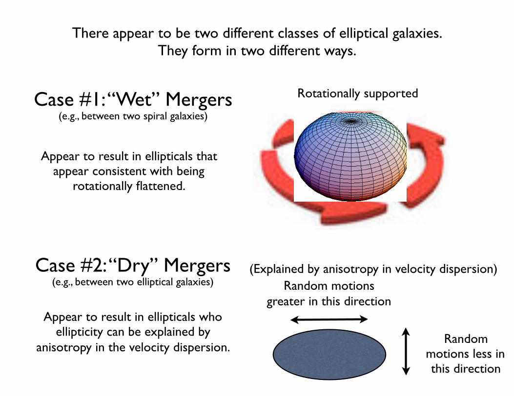
There appear to be two different classes of elliptical galaxies.They form in two different ways.

Case #1: “Wet” Mergers

Galaxy(with gas)

Galaxy(with gas)

(tends to occur more frequently for lower mass galaxies, when galaxy evolution less

advanced)

Case #2: “Dry” Mergers

Galaxy(without gas)

Galaxy(without gas)

(frequently occurs after many previous mergers, when the mass is higher)(e.g., between two elliptical galaxies)

(e.g., between two spiral galaxies)



Case #2: “Dry” Mergers(e.g., between two elliptical galaxies)


Appear to result in ellipticals that appear consistent with being

rotationally flattened.

Appear to result in ellipticals who ellipticity can be explained by

anisotropy in the velocity dispersion.

Random motions greater in this direction

Random motions less in this direction

Rotationally supported

(Explained by anisotropy in velocity dispersion)



Case #2: “Dry” Mergers(e.g., between two elliptical galaxies)


Appear to result in ellipticals that appear consistent with being

rotationally flattened.

Appear to result in ellipticals who ellipticity can be explained by

anisotropy in the velocity dispersion.

Lower Luminosity

Higher Luminosity Definition of Break radius

I( r) = Ib2(" -# )/$ (rb/r)

# [1+(r/rb)$ ](# -" )/$

rb = break radius where power-lawchanges slope and Ib is the surface brightness at the break

This is a five(!) parameter fit:" is the outer power-law slope# is the inner power law slope

$ defines the sharpness of thetransition

Break radius vs. Absolute magnitude

Shape of Ellipticals:

• Ellipticals are defined by En, where n=10!,

and !=1-b/a is the ellipticity.

• Note this is not intrinsic, it is observer

dependent!


• 3-D shapes – are ellipticals predominantly:

– Oblate: A=B>C (a flying saucer)

– Prolate: A>B=C (a cigar)

– Triaxial A>B>C (a football)

– Note A,B,C are intrinsic axis radii

• Want to derive intrinsic axial ratios from observed

– Can deproject and average over all possible observing angles to do

this

– Find that galaxies are mildly triaxial:

• A:B:C ~ 1:0.95:0.65 (with some dispersion ~0.2)

– Triaxiality is also supported by observations of isophotal twists in

some galaxies (would not see these if oblate or prolate)

Definition of Break radius

I( r) = Ib2(" -# )/$ (rb/r)

# [1+(r/rb)$ ](# -" )/$

rb = break radius where power-lawchanges slope and Ib is the surface brightness at the break

This is a five(!) parameter fit:" is the outer power-law slope# is the inner power law slope

$ defines the sharpness of thetransition

Break radius vs. Absolute magnitude


• Ellipticals are defined by En, where n=10!,

and !=1-b/a is the ellipticity.

• Note this is not intrinsic, it is observer

dependent!


• 3-D shapes – are ellipticals predominantly:

– Oblate: A=B>C (a flying saucer)

– Prolate: A>B=C (a cigar)

– Triaxial A>B>C (a football)

– Note A,B,C are intrinsic axis radii

• Want to derive intrinsic axial ratios from observed

– Can deproject and average over all possible observing angles to do

this

– Find that galaxies are mildly triaxial:

• A:B:C ~ 1:0.95:0.65 (with some dispersion ~0.2)

– Triaxiality is also supported by observations of isophotal twists in

some galaxies (would not see these if oblate or prolate)

No core in center of elliptical

Core in center of elliptical

Disky Isophotes

Boxy Isophotes

NOW new material for this week

Why do Elliptical Galaxies Look So Similar?

Why do Elliptical Galaxies All Look So Much Alike?

i.e., why do their surface brightness profiles approximately satisfya de-Vaucouleur law?

As we have seen from the first few lectures, there is a huge freedom in constructing collisionless systems that are in

equilibrium.

So, these profiles must arise in some other way!

Violent Relaxation

One way to set up the equilibrium phase-space structure in elliptical galaxies is through violent relaxation!

Under normal conditions, for equilibrium systems, we would expect minimal changes in phase space structure of galaxies

However, what would happen if there was a collision between two galaxies?

In this case, individual stars would experience a rapidly changing gravitational potential.

How would the time-varying gravitational potential affect individual particles?Violent Relaxation II

Particle gaines energy

Particle looses energy

No Relaxation

time

Individual particles can gain or lose energy (due to the changing potential)

Credit: van den Bosch

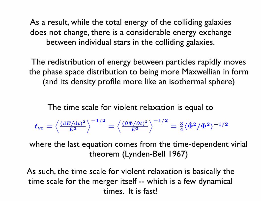
As a result, while the total energy of the colliding galaxies does not change, there is a considerable energy exchange

between individual stars in the colliding galaxies.

The redistribution of energy between particles rapidly moves the phase space distribution to being more Maxwellian in form

(and its density profile more like an isothermal sphere)

The time scale for violent relaxation is equal to

Violent Relaxation IIIA few remarks regarding Violent Relaxation:

• During the collapse of a collisionless system the CBE is still valid, i.e., thefine-grained DF does not evolve (df/dt = 0). However, unlike for a‘steady-state’ system, ∂f/∂t = 0.

• A time-varying potential does not guarantee violent relaxation. One canconstruct oscillating models that exhibit no tendency to relax: although theenergies of the individual particles change as function of time, the relativedistribution of energies is invariant (cf. Sridhar 1989).

Although fairly artificial, this demonstrates that violent relaxation requiresboth a time-varying potential and mixing to occur simultaneous.

• The time-scale for violent relaxation is

tvr =!

(dE/dt)2

E2

"−1/2=

!(∂Φ/∂t)2

E2

"−1/2= 3

4⟨Φ2/Φ2⟩−1/2

where the last step follows from the time-dependent virial theorem (seeLynden-Bell 1967).

Note that tvr is thus of the order of the time-scale on which the potentialchanges by its own amount, which is basically the collapse time. ◃ therelaxation mechanism is very fast. Hence the name ‘violent relaxation’

where the last equation comes from the time-dependent virial theorem (Lynden-Bell 1967)

As such, the time scale for violent relaxation is basically the time scale for the merger itself -- which is a few dynamical

times. It is fast!

The redistribution of energy between particles proceeds in such a way as to be independent of the mass of stars in

galaxies (since it only occurs due to time variations in the potential).

It therefore very different from what happens during collisional relaxation where there is a dependence on the

mass of the colliding stars (e.g., as in globular clusters where the most massive stars tend to collect in the center).

Let us consider one concrete example of a system undergoing violent relaxation

One such system is a cloud of particles that start out locally at rest.

How does this system evolve with time?

Gravity will cause this cloud of particles to collapse onto the center of the cloud...

This problem was initially considered by van Albada while working in Groningen (1982)

OutlineRange of timescales

Two-body relaxation timeViolent relaxationDynamical friction

Piet van der Kruit, Kapteyn Astronomical Institute Galactic dynamics: Timescales

How does such a system evolve with time?

van Albada (1982)

Here is a short movie illustrating such a collapsing cloud:

Note that the flow is initially very uniform and ordered! After collapse, individual stars have a wide range of

velocities and energies!

How does this re-distribution of energy look for this collapsing cloud?

20-3-12see http://www.strw.leidenuniv.nl/˜ franx/college/galaxies12 12-c02-5

Furthermore, such distributions are also naturally triax-ial.

Interestingly, mergers also produce profiles which are


rather similar. This is maybe not too surprising (theprofiles are already a bit similar at the start) - and ap-parently there is enough violent relaxation during themerger to smooth things out. Here are the profilesas derived by Hopkins et al (2008) from a large set ofmerger simulations

Intrinsic correlations

We have seen that ellipticals can be scaled up anddown as far as the equilibrium laws are concerned. In

Initial Distribution

At intermediate time

At late time

(energy)

# of stars

Remarkably, it was found that the final density profile of the equilibrium system that formed from the collapsing cloud

followed a R1/4 law.

densityinitial

after collapse

R1/4 relation

What is the final density profile for this collapsing cloud?

Such density distributions that result from such a collapse are also naturally triaxial in form.








Here are projections of the density distribution of stars in the xy, xz, and yz planes.

Additional smoothing out of the phase space distribution is provided by the process of phase mixing:Phase Mixing I

Consider circular motion in a disk with Vc(R) = V0 = constant. Thefrequency of a circular orbit at radius R is then

ω = 1T

= V0

2πR

Thus, points in the disk that are initially close will separate according to

∆φ(t) = ∆!

V0

Rt"

= 2π∆ωt

We thus see that the timescale on which the points are mixed over theiraccessible volume in phase-space is of the order of

tmix ≃ 1∆ω

where due to differences in the oscillation frequencies for different stars in a collisionless system, stars spread out to

more completely fill phase space.








What about the merger between two galaxies?

Amazingly, one finds very similar density profiles to what one finds for the collapsing clouds. Here are some results

from Hopkins et al. (2008):

These merging galaxies also largely follow R1/4 density profiles.

surface brightness

What about the merger between two galaxies?

Amazingly, one finds very similar density profiles to what one finds for the collapsing clouds. Here are some results

from Hopkins et al. (2008):

These merging galaxies also largely follow R1/4 density profiles.








surface brightness

surface brightness

Intrinsic Correlations between Galaxy Properties


reality, they span a relatively narrow range in proper-ties. The figure below shows the distribution.

The figure on the top right shows the relation betweenabsolute magnitude and velocity dispersion. This isthe Faber Jackson relation, the equivalent of the Tully-Fisher relation for spirals.


The other figures show the additional relations betweensize (Re), surface brightness (< µe >), and velocitydispersion (σ). If we combine these 3 properties op-timally, we find a very tight relation (at the bottomright).

R ∝ σ1.4µ−0.9e

This relation is called the Fundamental Plane (thereis not too much fundamental about it). It is muchtighter than the Faber Jackson relation. What causessuch a relation ?

Origin of the Fundamental Plane

The fundamental plane can best be understood as arelation between the mass-to-light ratio and the massof the galaxy. Use the fundamental plane to removethe “light” term in the mass-to-light ratio:

M

L∝

M

R2eµe

∝

M

R−1.1e σ1.5R2

e

∝

M

M0.75R0.15e

∝

∝ M0.25R−0.15e

Here we used M ∝ Reσ2 . We see that the mass-to-light ratio is a function of mass (and a tiny bit ofeffective radius). This is probably due to the stellarpopulations in early-type galaxies: the metallicity, andpossibly the age of the galaxies are a function of itsmass. If so, one would automatically expect that themass-to-light ratio is a function of the mass.

Some people also think that more aspects play a rolethan just the stellar populations. It could be, for ex-ample, that the profiles of the galaxies vary systemat-ically with mass - so that the simple equations which

Strong correlations are observed between the masses, sizes, and velocity dispersions of elliptical galaxies.

average surface brightness

half-light radius

i.e., radius containing half of the

light

As we noted earlier, such correlations would not need to be present for a generic collisionless system and tell us something fundamental

about the formation of galaxies themselves.






R ∝ σ1.4µ−0.9e




M

L∝

M

R2eµe

∝

M

R−1.1e σ1.5R2

e

∝

M

M0.75R0.15e

∝

∝ M0.25R−0.15e




absolute magnitude inside the half-light radius

velocity dispersion








R ∝ σ1.4µ−0.9e




M

L∝

M

R2eµe

∝

M

R−1.1e σ1.5R2

e

∝

M

M0.75R0.15e

∝

∝ M0.25R−0.15e




velocity dispersion

average surface brightness







R ∝ σ1.4µ−0.9e




M

L∝

M

R2eµe

∝

M

R−1.1e σ1.5R2

e

∝

M

M0.75R0.15e

∝

∝ M0.25R−0.15e




half-light radius

velocity dispersion

Notice how much tighter the relationship can become

if one combines the quantities in the appropriate

fashion!


These correlations are such that galaxies populate a fundamental plane in these parameters, so that if you know two of the following three

variables for a galaxy, you can determine the third.






R ∝ σ1.4µ−0.9e




M

L∝

M

R2eµe

∝

M

R−1.1e σ1.5R2

e

∝

M

M0.75R0.15e

∝

∝ M0.25R−0.15e



where R is the size (radius), σ is the velocity dispersion, and μ is the galaxy surface brightness.

The properties of galaxies occupy a two dimensional plane in the three dimensional parameter space.

Fundamental Plane (3-D)

Here is an illustration of such a two-dimensional surface embedded in a

three-dimensional space.

How shall we interpret this fundamental plane relation?

Let us interpret in terms of the mass to light ratio of galaxies:

M

L=

M

µeRe2

µe ~ σ1.5 Re-1.1

=M

σ1.5 Re-1.1 Re2

M ~ σ2 Re

M0.75 ~ σ1.5 Re0.75

=M

M0.75 Re-0.75Re-1.1 Re2= M0.25Re-0.15

From virial relation:

The fundamental plane relation implies that the mass-to-light ratio scales as M0.25 Re-0.15.

It is unclear what causes this mass dependence. It could be due to the stellar populations (i.e., that the baryonic component in massive

galaxies have higher mass-to-light ratios) or due to dark matter playing a larger dynamical role in more massive galaxies

What about Baryonic Gas in Ellipticals? Do they have any?

Yes -- lots of hot ionized gas!

Luminosity of the hot ionized gas scales

approximately as the optical luminosity

squared!

Hot ionized gas appears to originate partially from mass

loss from AGB stars.

Heating is from SNe and movement of stars through

gas

Total gas mass ranges from 109 to 1011

solar masses

Hot Gas in Ellipticals

  LX goes as LB1.6-2.3

(empirical relation)   ρ goes as r-3/2

  Mgas~ 109–1011M

  Origin of hot gas   Reservoir   External   Internal:

  Mass return from AGB stars ~1.5 x 1011Myr-1L

-1

  Heated by Sne (what kind?), thermal motion of stars at 200-300 km s-1

Radial distribution

What about Baryonic Gas in Ellipticals? Do they have any?

Occasionally there is cool gas

However, most of the time it is outside the center of a gas.

It is expected to be rare, since elliptical galaxies do notundergo much star formation.

Dark Matter Halos

Dark Matter Halos

Two Key Steps in Galaxy Formation

1. Gravitational Collapse2. Cooling of Baryons to Center

Form of the Collapsed Dark Matter Halo(step #1 in galaxy formation process) can have an

important impact on the structure and properties of galaxies...

Let’s derive the key relations between the mass, radius, and velocity dispersion in halos

When a halo collapses -- how does ρhalo compare to ρcritical ?

Theory of Dark Matter Halos

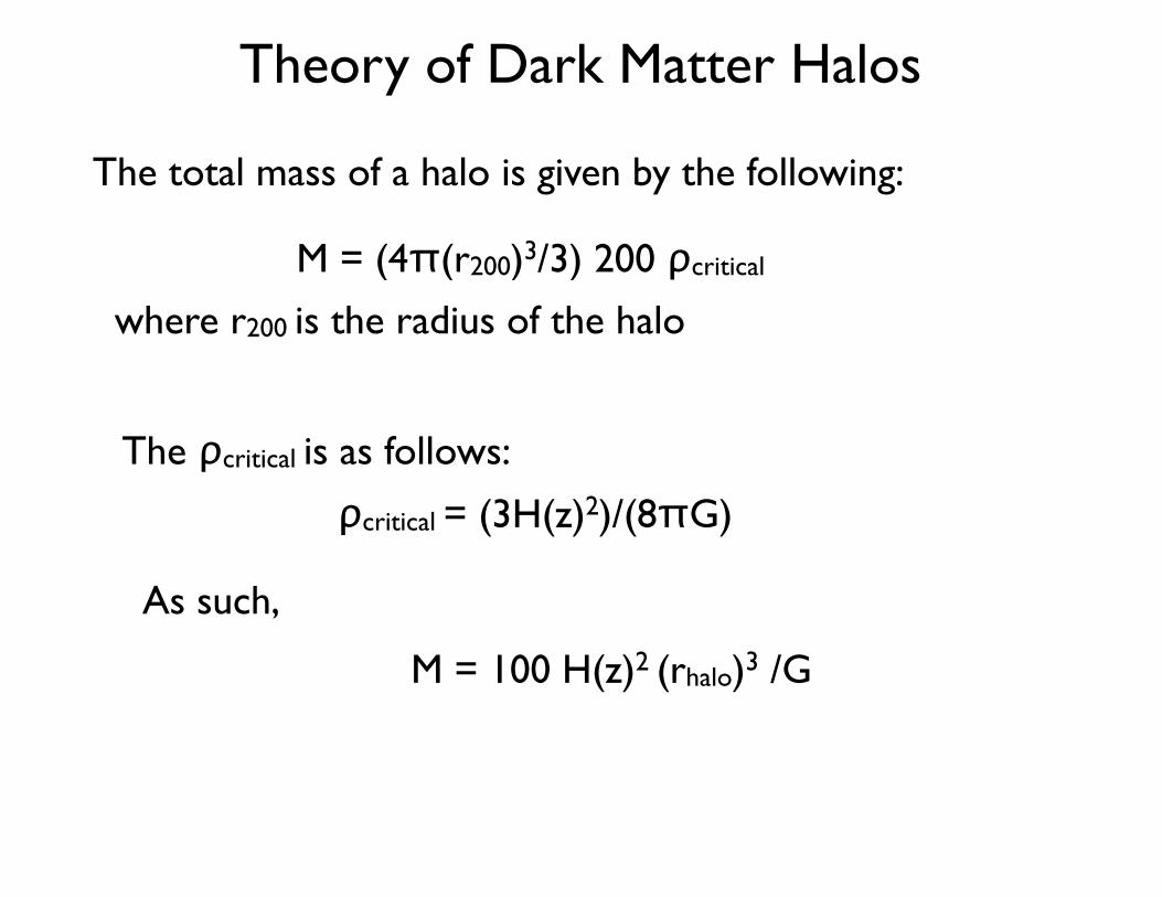
M = (4π(r200)3/3) 200 ρcritical


The total mass of a halo is given by the following:

ρcritical = (3H(z)2)/(8πG)

The ρcritical is as follows:

As such,

M = 100 H(z)2 (rhalo)3 /G

where r200 is the radius of the halo


(V200)2 = GM/r200

From the virial relationship:

One can write expressions for the mass and radius of the haloin terms of the circular velocity and the Hubble constant:

M = (V200)3 / 10GH(z)

r200 = V200/10H(z)

The Hubble “constant” H(z) increases towards higher redshifts, effectively scaling as (1+z)3/2 at very high redshifts.

Halos of a given mass are more compact at high redshift.

Navarro-Frenk-White Density Profiles


4. Structure of Dark Matter halos

Obviously, we cannot observe the dark matter halosdirectly - but we can measure the total density profilesof clusters, and we can check in our simulations whatwe expect for dark matter halos.

4.1 Theory of halo collapse

We define a halo as a region in which the density islarger than 200 times the critical density ρcr. This def-inition serves well to describe the collapsed part of thehalo.Hence the mass M is given by

M =4π

3r3

200200ρcr

Since the critical density is given by

ρcr(z) =3H2(z)

8πG

we find

M =100r3

200H2(z)

G

Hence the halo mass and the size are uniquely related -and the relation changes as a function of redshift.The virial velocity of the halo is the circular velocity atthe virial radius

V 2

200 =GM

r200


Hence the halo mass, virial radius, and virial velocityare related by

M =V 3

200

10GH(z)

r200 =V200

10H(z)

The Hubble constant H(z) increases with lookbacktime. Hence at higher redshift, the size of a halo of agiven mass is smaller than the size of a halo with thesame mass at low redshift. Halos are more compactand denser at high redshift, which is exactly what weexpect, as the density of the universe is higher at highredshift (by (1 + z)3).Simulations show that the density profiles of halos arewell approximated by a Navarro Frenk White profile(1997):

ρ(r) =ρs

(r/rs)(1 + r/rs)2

where ρs and rs are scaling parameters. Hence at verysmall radii (r < rs), ρ ∝ r−1, and at large radii (r >rs) ρ ∝ r−3. At rs, the slope of the density profilebends over.We define a concentration parameter c by c = r200/rs.It is easy to show that

ρs =200

3ρcr(z)

c3

ln(1 + c) − c/(1 + c)

Hence the profile of the halo is completely determinedby the mass M (or equivalently, the radius r200), andthe concentration paramater c.

Simulations show that collapsed halos approximately have the following density profile:

where rs and ρs are some scaling parameters.

At small radii (r < rs), the density profile ρ scales approximately as r−1

and at large radii (r > rs), the density profile ρ scales approximately as r−3

At r ~ rs, the density profile ρ changes slope


Simulations show that the concentration index is stronglycorrelated with the mass and the redshift. Approxi-mately

c ∝

M−1/9

M∗

(1 + z)−1

where M∗ is the charateristic halo mass at a givenmass (similar to the Schechter L∗ for the luminosityfunction of galaxies, and z is the redshift of the halo.

Hence low mass halos have higher concentration.

The figures below shows the fits to halos from simula-tions


Here are some examples of the density profiles from simulations:

SCDM = standard cold dark matter

(no dark energy)

ΛCDM = cold dark matter with

dark energy

rs



c ∝

M−1/9

M∗

(1 + z)−1




13-4-12see http://www.strw.leidenuniv.nl/˜ franx/college/galaxies12 12-c04-4Here are some examples of the density profiles from simulations:

SCDM = standard cold dark matter

(no dark energy)

ΛCDM = cold dark matter with

dark energy


Define concentration parameter c = r200 / rs


4. Structure of Dark Matter halos

Obviously, we cannot observe the dark matter halosdirectly - but we can measure the total density profilesof clusters, and we can check in our simulations whatwe expect for dark matter halos.

4.1 Theory of halo collapse

We define a halo as a region in which the density islarger than 200 times the critical density ρcr. This def-inition serves well to describe the collapsed part of thehalo.Hence the mass M is given by

M =4π

3r3

200200ρcr

Since the critical density is given by

ρcr(z) =3H2(z)

8πG

we find

M =100r3

200H2(z)

G

Hence the halo mass and the size are uniquely related -and the relation changes as a function of redshift.The virial velocity of the halo is the circular velocity atthe virial radius

V 2

200 =GM

r200


Hence the halo mass, virial radius, and virial velocityare related by

M =V 3

200

10GH(z)

r200 =V200

10H(z)

The Hubble constant H(z) increases with lookbacktime. Hence at higher redshift, the size of a halo of agiven mass is smaller than the size of a halo with thesame mass at low redshift. Halos are more compactand denser at high redshift, which is exactly what weexpect, as the density of the universe is higher at highredshift (by (1 + z)3).Simulations show that the density profiles of halos arewell approximated by a Navarro Frenk White profile(1997):

ρ(r) =ρs

(r/rs)(1 + r/rs)2

where ρs and rs are scaling parameters. Hence at verysmall radii (r < rs), ρ ∝ r−1, and at large radii (r >rs) ρ ∝ r−3. At rs, the slope of the density profilebends over.We define a concentration parameter c by c = r200/rs.It is easy to show that

ρs =200

3ρcr(z)

c3

ln(1 + c) − c/(1 + c)

Hence the profile of the halo is completely determinedby the mass M (or equivalently, the radius r200), andthe concentration paramater c.

Requiring the total mass in the halo is equal to 200 ρcrit(z) (4π/3 (r200)3), one can show that

so that the density profile of a halo is completely determined by its mass and concentration parameter c.


From simulations, one finds that the concentration parameter c for a halo is closely related to its formation redshift:



c ∝

M−1/9

M∗

(1 + z)−1





Lower mass halos have higher concentration parameters.

Navarro-Frenk-White Density Profiles4 J. C. Munoz-Cuartas et al.

has a smoothing effect, not all unrelaxed haloes have a highρrms. In order to circumvent these problems, we combine thevalue of ρrms with the xoff parameter, defined as the distancebetween the most bound particle (used as the center for thedensity profile) and the center of mass of the halo, in unitsof the virial radius. This offset is a measure for the extentto which the halo is relaxed: relaxed haloes in equilibriumwill have a smooth, radially symmetric density distribution,and thus an offset that is virtually equal to zero. Unrelaxedhaloes, such as those that have only recently experienceda major merger, are likely to reveal a strongly asymmetricmass distribution, and thus a relatively large xoff . Althoughsome unrelaxed haloes may have a small xoff , the advan-tage of this parameter over, for example, the actual virialratio, 2T/V , as a function of radius (e.g. Maccio, Murante& Bonometto 2003), is that the former is trivial to evaluate.Following Maccio et al. (2007), we split our halo sample intounrelaxed and relaxed haloes. The latter are defined as thehaloes with ρrms < 0.5 and xoff < 0.07. About 70% of thehaloes in our sample qualify as relaxed haloes at z = 0.

To check for the effect of changing the definition of re-laxed haloes, we have computed the median concentration(as shown in the next section) using different values of xoff .Changing the value of this parameter by 25% (above andbelow 0.07) induces changes no larger than 5% in the me-dian concentration of dark matter haloes. We conclude thatchoosing xoff = 0.07 our results are robust enough againstvariations in the definition of relaxed population of haloes.In what follows we will just present results for haloes whichqualify as relaxed.

3 CONCENTRATION: MASS AND REDSHIFT

DEPENDENCE

In figure 1 we show the median cvir−Mvir relation for relaxedhaloes in our sample at different redshifts. Haloes have beenbinned in mass bins of 0.4 dex width, the median concentra-tion in each bin has been computed taking into account theerror associated to the concentration value (see 2.1.1, andM08). In our mass range the cvir−Mvir relation is well fittedby a single power law at almost all redshifts. Only for z = 2we see an indication that the linearity of the relation in logspace seems to break, in agreement with recent findings byKlypin et al. (2010).

The best fitting power law can be written as:

log(c) = a(z) log(Mvir/[h−1 M⊙]) + b(z) (5)

The fitting parameters a(z) and b(z) are functions ofredshift as shown in figure 2. The evolution of a and b canbe itself fitted with two simple formulas that allow to recon-struct the cvir −Mvir relation at any redshifts:

a(z) = wz −m (6)

b(z) =α

(z + γ)+

β(z + γ)2

(7)

Where the additional (constant) fitting parameters havebeen set equal to: w = 0.029, m = 0.097, α = −110.001,β = 2469.720 and γ = 16.885. Figure 3 shows the recon-struction of the cvir−Mvir relation for different mass bins asa function of redshift using the approach described above. Itshows that our (double) fitting formulas are able to recover

0.5

0.6

0.7

0.8

0.9

1

1.1

1.2

10 10.5 11 11.5 12 12.5 13 13.5 14 14.5 15

log 1

0(c v

ir)

log10(Mvir[M⊙ h-1])

z=0.00z=0.23z=0.38z=0.56z=0.80z=1.12z=1.59z=2.00

Figure 1. Mass and redshift dependence of the concentrationparameter. The points show the median of the concentration ascomputed from the simulations, averaged for each mass bin. Linesshow their respective linear fitting to eq. 5.

the original values of the halo concentration with a precisionof 5%, for the whole range of masses and redshifts inspected.It has been shown by Trenti et al. (2010) that using Nvir be-tween 100 and 400 particles is enough to get good estimatesfor the properties of halos, nevertheless in order to look forsystematics we re-computed cvir varying the minimum num-ber of particle inside Rvir, using 200, 500 and 1000 particles.No appreciable differences (less than 2%) were found in ourresults for the median. We also checked that our results donot change notably by changing the definition of “relaxed”haloes (i.e. changing the cut in xoff or ρrms).

It is interesting to compare our results with M08, whichshares some of the simulations presented in this work. Ourresults for the cvir −Mvir relation at z = 0 are slightly dif-ferent to those presented in M08: we found a = −0.097 andb = 2.155, while M08 found a = −0.094 and b = 2.099.The difference is less than 3%, and it is mainly due to lowmass haloes. In this work we included three new simulations,B30, B90 and B3002. Two of these (B30 and B90) increasethe statistics of our halo catalogs at the low mass end, pro-viding a better determination of the cvir −Mvir relation forM ≈ 1011h−1 M⊙. We are confident that the inclusion thosenew simulations led to an improvement over the results ofprevious works.

3.1 Understanding the concentration evolution

We want now to explore in more detail the physical mecha-nism driving the mass and redshift dependence of the con-centration parameter, this understanding could take us to abetter interpretation of the time evolution of the dark mat-ter density profile. As cvir is defined as the ratio between Rvir

and rs we will look at the time evolution of those quantitiesfor different halo masses, and try to see if we can extractsome physical insights about the evolution of cvir.

c⃝ 2010 RAS, MNRAS 000, 1–11

Munoz-Cuartas et al. 2010

Let’s also look at the rotational curves:



c ∝

M−1/9

M∗

(1 + z)−1





Does this make sense in terms of

V2 ~ GM(R)/R ?

Collapsed Halos: Comparison with the Observations

First -- we look at the structure of the dark matter halofor very massive collapsed halo (M ~ 1014 - 1015 Msolar)

i.e., as appropriate for galaxy clusters


4.2 Comparison to observations

The easiest test to make, is to compare the densityprofiles of clusters to those of the simulations (theNFW profiles, and variants).

Below we show the comparison of mass profiles derivedfrom X-ray data to those of NFW profiles:

It is remarkable how good the fit is, and the concen-tration index is well within the limits expected for theclusters.

Another (simpler) way to do this, is by looking at thedistribution of the galaxies within the clusters. Again,a good fit is found:


Radial Profile

Halos of Galaxy Clusters: Comparison against the Observations

Mass / M200

Radius / r200

Information from x-ray profiles

Mass Profile comes assuming hydrostatic equilibirum

Pressure gradient balancesgravitational forces!

XMM Newton Data of 10 Clusters









Do the 10 clusters from previous page fit the

theoretical concentration vs. mass relationship?

Cluster Mass

Concentration



c ∝

M−1/9

M∗

(1 + z)−1






We can also use the apparent surface

density of galaxies within clusters vs.

radius to probe the density profile.















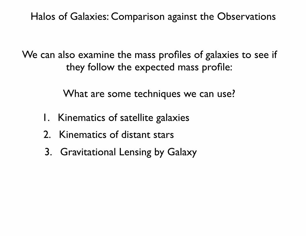
Halos of Galaxies: Comparison against the Observations

We can also examine the mass profiles of galaxies to see ifthey follow the expected mass profile:

1. Kinematics of satellite galaxies

2. Kinematics of distant stars

3. Gravitational Lensing by Galaxy

What are some techniques we can use?

Kinematics of Satellite Galaxies:13-4-12see http://www.strw.leidenuniv.nl/˜ franx/college/galaxies12 12-c04-7

Halo Structure of galaxies

For galaxies, it is much harder to measure the darkmatter halo structure. Gas velocity curves do not ex-tend far enough. Just as an exercise, estimate the virialradius of a galaxy like our own Milky Way. Just as-sume that V200 = 150km/s. For r200 we would derive150/(10 ∗ 70) Mpc = 210 kpc, very much beyond thesizes of (gas) disks.

Hence we need different tracers to estimate the massesand mass profiles. Options are:

• 1. kinematics of satellite galaxies

• 2. kinematics of very distant stars

• 3. deflection of light

Below we show some examples.

1) Satellites. The SDSS project has measured a largenumber of velocities of galaxies. Some of these galax-ies are close together on the sky, and sometimes, thesegalaxies are bound. Usually, a galaxy has only 1 satel-lite galaxy with a measured velocity. To still allow themeasurement of a signal, we combine all the satellitegalaxy-main galaxy pair. We restrict the main galaxiesto those galaxies with similar luminosity.

By careful analysis, the velocity dispersion of the satel-lite system can be measured. Prada et al (2003) foundthis results:


The results are very nicely described by an NFW pro-file.

2. Kinematics of very distant stars. This method ismost easily applied to our own galaxy (but studies ofexternal galaxies are coming !). A very recent exampleis shown below (Xue et al. 2008):

One method is to take advantage of the satellite companions found around galaxies in the nearby local universe as

a probe of kinematics.

Unfortunately, one only tends to find one such satellite galaxy per central

galaxy (with a measured velocity along the line of sight), so it is not possible to

make a reliable measurement using individual galaxies.

To make progress, one needs to treat these galaxies as orbitting around

some “composite average” galaxy.

Prada et al. 2003

Velocity

Radius (kpc)

Data

Results are in good agreement with an NFW profile

NFW

Most easily applied to our own galaxy.

Kinematics of Distant Stars


The authors were able to measure the velocity disper-sion to 60kpc. This is a record - but still much smallerthan the virial radius r200 which is at the level of 200kpc.

3. Gravitational deflection of light. This method relieson the bending of light through gravity. A beautifulexample is when the galaxy produces an Einstein ringof a source behind it.


In this case, two galaxies are located nearly preciselybehind another. The mass inside the ring is well de-termined. However, this method does not extend tovery large radii - one would have to analyze the weakerdeflections. This is possible, but much harder.

An example is shown below (van Uitert et al 2011, AA534, 14). In this case, the shapes of many backgroundgalaxies are averaged together. The measured γ isthe average elongation of background galaxies. Thisis mostly due to the weak gravitational lensing by theforeground galaxy. The measured signal can be com-pared to the theoretical expectation.

One use of this method shown below (Xue et al. 2008)

Applied to 60 kpc! (which is nevertheless smaller than 200 kpc:

which is approximately the halo radius)

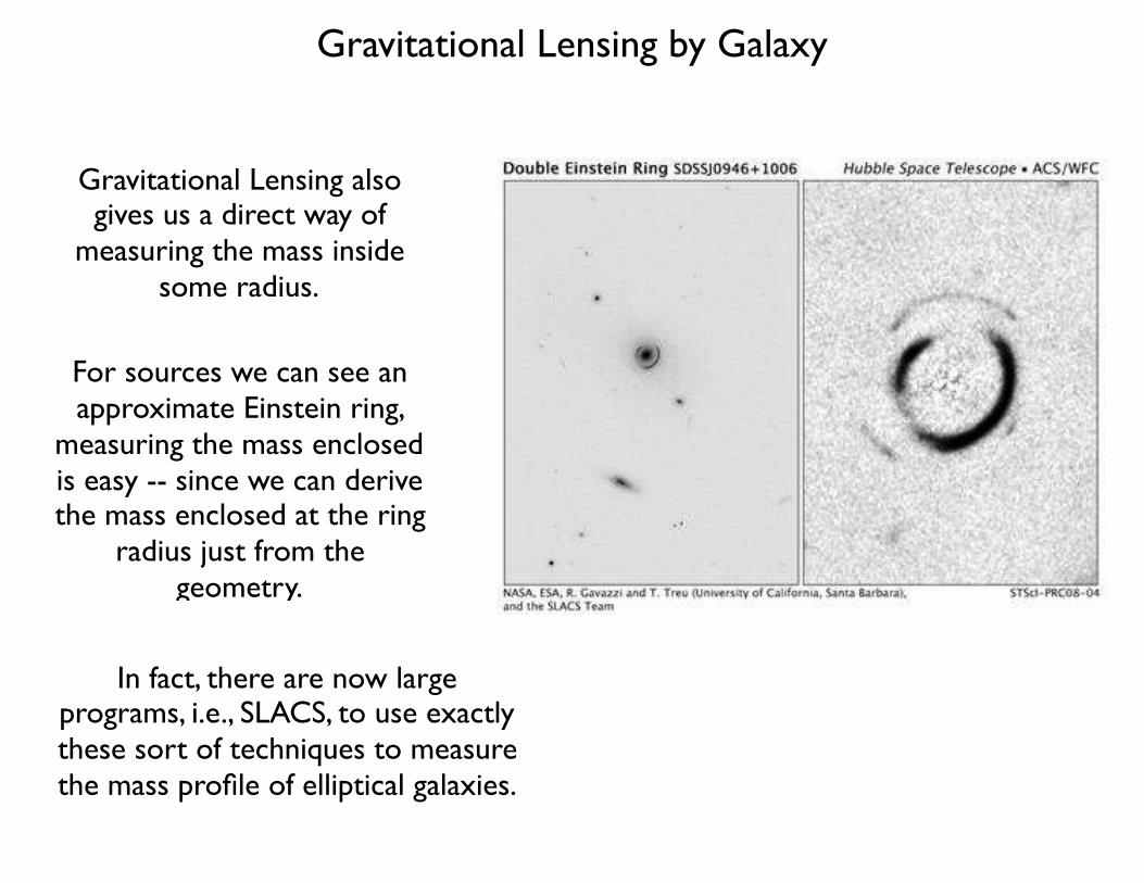
Gravitational Lensing also gives us a direct way of

measuring the mass inside some radius.

Gravitational Lensing by Galaxy


The authors were able to measure the velocity disper-sion to 60kpc. This is a record - but still much smallerthan the virial radius r200 which is at the level of 200kpc.

3. Gravitational deflection of light. This method relieson the bending of light through gravity. A beautifulexample is when the galaxy produces an Einstein ringof a source behind it.


In this case, two galaxies are located nearly preciselybehind another. The mass inside the ring is well de-termined. However, this method does not extend tovery large radii - one would have to analyze the weakerdeflections. This is possible, but much harder.

An example is shown below (van Uitert et al 2011, AA534, 14). In this case, the shapes of many backgroundgalaxies are averaged together. The measured γ isthe average elongation of background galaxies. Thisis mostly due to the weak gravitational lensing by theforeground galaxy. The measured signal can be com-pared to the theoretical expectation.

For sources we can see an approximate Einstein ring,

measuring the mass enclosed is easy -- since we can derive the mass enclosed at the ring

radius just from the geometry.

In fact, there are now large programs, i.e., SLACS, to use exactly these sort of techniques to measure the mass profile of elliptical galaxies.

The Sloan Lens ACS Survey (SLACS)

Cols: T. Treu (UCSB), L. Koopmans (Kapteyn),A. Bolton (CfA), S. Burles (MIT), L. Moustakas (JPL)

Spectroscopic selection (spurious emission lines), then HST follow-up imaging for confirmation and for accurate modeling

R. Gavazzi, SBastro07, 3




SLACS sample

Despite some success in this regard, it is not always easy to find

large numbers of galaxies with Einstein rings.


An alternate technique is to measure the average impact of

gravitational lensing of the shapes of galaxies.

Impact of gravitational lensing is to introduce subtle change in the shape of galaxies on average (so

elongated along an angle tangential to the galaxy)

13-4-12see http://www.strw.leidenuniv.nl/˜ franx/college/galaxies12 12-c04-11 13-4-12see http://www.strw.leidenuniv.nl/˜ franx/college/galaxies12 12-c04-12

Problems with dark matter halos and realgalaxies

Generally, two problems exist: some galaxies may haverather large central cores (larger than expected in theNFW profiles), and the dark matter halos in the simu-lations have too many “sub-halos”.

• Cores

Low surface brightness galaxies have rotation curveswhich rise slowly. This is unexpected for galaxies withNFW halos. Naray et al 2007 (arxiv: 0712.0860) showthis result:

Fits with NFW profiles are hard. The rise of the rota-tion curve is too slow:

By looking at many foreground galaxies and determining the average change in shape of many background galaxies, we can measure the mass profile of the galaxy.

van Uitert et al. 2011

Such averaging is required because

background galaxies have random shapes

and orientations.

However, averaging over enough galaxies, one can overcome the

random component.

Challenges / Issues with our standard model for the collapsed dark matter halos

Cores of Halos

What can we infer about the cores of dark matter halos from the observations?

Where should we look?

Almost all collapsed halos have baryons cooling and falling towards their centers. These baryons will change the mass

profile of the original collapsed halo.

V(R)2 R / G ~ M(R) ~ MDARK(R) + MCOOL(R)

Basically, we have the following situation:

To obtain best constraints on MDARK(R), we need MCOOL(R) to be as small as possible.

Cores of Halos

For which galaxies would we expect the halos to be the least affected by the baryons cooling to the centers?

For which galaxies, will MCOOL(R) be the smallest?

spinning moderate speed spinning fast

after cooling after cooling

intermediate size,more dense disk galaxy

large, lower density galaxy disk

higher surface brightness lower surface brightness

Here are two galaxies where the baryonic component hasdifferent angular momentum. For which case, can we get a

cleaner look at the dark matter halo?




• Cores






• Cores






• Cores



Cores of Halos

What would infer about the mass profile of a halo where the circular velocity appears to rise linearly with radius?

Using the relation M = V(R)2 R / G,

we would infer that M ∝ R3 or ρ ~ independent of radius

But for NFW, we would expect ρ ∝ r−1 at small radii

Galaxies: Structure, Dynamics, and...

Documents

Transcript of Galaxies: Structure, Dynamics, and...