Antranik A. Siranosian1

e-mail: aasiranosian@gmail.com

Miroslav Krstic

Andrey Smyshlyaev

Department of Mechanical and

Aerospace Engineering,

University of California, San Diego,

La Jolla, CA 92093

Matt BementLos Alamos National Laboratory,

Los Alamos, NM 87545

Gain Scheduling-InspiredBoundary Control for NonlinearPartial Differential EquationsWe present a control design method for nonlinear partial differential equations (PDEs)based on a combination of gain scheduling and backstepping theory for linear PDEs. Abenchmark first-order hyperbolic system with an in-domain nonlinearity is consideredfirst. For this system a nonlinear feedback law, based on gain scheduling, is derived ex-plicitly, and a proof of local exponential stability, with an estimate of the region of attrac-tion, is presented for the closed-loop system. Control designs (without proofs) are thenpresented for a string PDE and a shear beam PDE, both with Kelvin–Voigt (KV) damp-ing and free-end nonlinearities of a potentially destabilizing kind. String and beam simu-lation results illustrate the merits of the gain scheduling approach over the linearizationbased design. [DOI: 10.1115/1.4004065]

Keywords: gain scheduling, PDE backstepping, boundary control, nonlinear control,stabilization, motion planning, hyperbolic PDEs, wave equation, string, beam

1 Introduction

The stabilization of nonlinear partial differential equations(PDEs) is an important area in control design motivated by real-world applications in the areas of thermal, reaction, fluid, structural,and plasma systems. Several control design methods for PDEs havebeen reported in the literature. We discuss only those that are rela-tively broadly applicable rather than being for a single specificPDE. Finite-dimensional backstepping methods were used for thedesign of stabilizing boundary controllers for spatially discretizedparabolic PDEs in Refs. [1–3]. Statistical-based model reductiontechniques were presented in Refs. [4–6]. Nonlinear model reduc-tion and input–output feedback linearization for quasilinear first-order hyperbolic and parabolic systems were presented in Ref. [7].Passivity based exponentially stabilizing control design and a flat-ness based approach for trajectory generation for flexible structureswere presented in Ref. [8]. Feedforward and feedback controllersbased on formal power series parameterization and summationmethods for stabilization and tracking for nonlinear PDEs were pre-sented in Ref. [9]. A gain scheduling approach for nonlinear PDEsin Ref. [10] used a linearization based approach, where controllerswere designed for the finite-dimensional approximation of the sys-tem linearized about a family of operating points. An approach forfull state feedback linearization for a broad class of nonlinear para-bolic partial integro-differential equations (PIDEs) was presented inRefs. [11,12], where the nonlinear feedback operators are con-structed using Volterra series in the spatial variable.

This paper presents a gain scheduling inspired control designfor nonlinear PDEs based on the backstepping approach for linearPDEs. Gain scheduling [13–22] is a technique that replaces a fullynonlinear control design (such as, for example, backstepping orforwarding, which yield global stability) with the design of a fam-ily of linear controllers that are implemented according to a sched-uling signal. It requires linearizing the plant about a family ofoperating points (for example, see Refs. [18,23,24]) or the formu-lation of the model in a quasi-linear parameter varying (LPV)form (for example, see Refs. [18,21]), such that linear control

tools can be applied. PDE backstepping [25] is an approach forthe design of boundary controllers for infinite dimensional PDEmodels without discretization or model reduction. As a form ofmodel reference control for infinite dimensional systems, statetransformations relating a closed-loop system to a target systemare used to design stabilizing controllers.

Here the design of a stabilizing controller begins by writing thePDE model in a form to which gain scheduling techniques apply.Once in the appropriate form, gain scheduled PDE backsteppingtransformations—similar to standard PDE backstepping transfor-mations in structure, but employing state-dependent transforma-tion gains—are used to relate the nonlinear PDE model to a targetsystem. Unlike typical gain scheduled controllers, where eitherthe controller or its parameters are scheduled, the resulting con-trollers in this work are applied as nonlinear controllers (linearcontrollers with “continuously scheduled” state-dependent param-eters). While not as powerful as the exactly linearizing nonlinearPDE backstepping boundary controllers in Refs. [11,12], gainscheduling controllers are a simpler and much more manageabledesign alternative for the challenging problem of nonlinear PDEcontrol, with performance advantages over linearization baseddesigns. Note that this work does not pursue the proof of existenceand uniqueness of solutions for the PDEs considered, and the con-trol designs are done assuming unique solutions exist.

We first present an explicit gain scheduling based control designfor a benchmark first-order hyperbolic PDE with a boundary-value-dependent in-domain nonlinearity, which is an extension of theresult in Ref. [26]. For this benchmark system we present a detailedanalysis of local exponential stability, with an estimate of the regionof attraction. Even for this relatively simple nonlinear PDE system,the analysis is quite complex and highlights the issues that onewould face in performing a stability analysis for more complex non-linear PDEs with gain scheduling controllers. These issues includethe construction of Lyapunov functionals using nonlinear backstep-ping transformations, the bounding of nonlinear terms left uncom-pensated in the gain scheduling approach, and perhaps most impor-tantly, the choice of system norms and the derivation of stabilityestimates and regions of attraction in high enough Sobolev norms tocapture the effect of nonlinear perturbations in the stability analysis.

We then turn our attention to some relevant basic mechanicalPDE systems—the string and shear beam PDEs with Kelvin–Voigt damping and boundary-displacement-dependent free-end

1Corresponding author.Contributed by the Dynamic Systems Division of ASME for publication in the

JOURNAL OF DYNAMIC SYSTEMS, MEASUREMENT, AND CONTROL. Manuscript receivedDecember 12, 2008; final manuscript received February 26, 2011; published onlineAugust 1, 2011. Assoc. Michael A. Demetriou.

Journal of Dynamic Systems, Measurement, and Control SEPTEMBER 2011, Vol. 133 / 051007-1Copyright VC 2011 by ASME

Downloaded 03 Aug 2011 to 137.110.37.145. Redistribution subject to ASME license or copyright; see http://www.asme.org/terms/Terms_Use.cfm

nonlinearities. These designs are the extensions of results for thestring [27–30] and shear beam [29–32]. The merits of thesedesigns are highlighted by simulation. Motivation for these sys-tems comes from shake table control and from atomic force mi-croscopy. In a particular shake table control problem, the tableprovides boundary actuation to a structure in order to impart adesired reference trajectory at some point near its free-end, whichpossibly exhibits nonlinear behavior. In atomic force microscopy,the base of a cantilevered beam is actuated to stabilize a probe atits free-end, which interacts nonlinearly with the sample surface.

This work introduces a completely new framework for PDEbackstepping designs, though the designs do employ past resultsfor linear PDEs. This new approach allows for the design ofexplicit nonlinear controllers for PDEs, rather than controllersgiven in the form of a nonlinear Volterra series, as in Refs. [11,12]. Also, the analysis techniques introduced for the nonlinearhyperbolic PDE are far beyond those previously employed inbackstepping designs for linear PDEs.

The paper is organized as follows. Section 2 presents the gainscheduling based control design for a benchmark first-orderhyperbolic PDE with boundary-value-dependent in-domain nonli-nearity, and the proof of stability for the resulting closed-loop sys-tem. Sections 3 and 4 present the control design and simulationresults for a string with Kelvin–Voigt damping and boundary-dis-placement-dependent free-end nonlinearity. Section 5 presents thecontrol design for the shear beam with Kelvin–Voigt damping andboundary-displacement-dependent free-end nonlinearity. Section6 presents simulation results for the Timoshenko beam with Kel-vin–Voigt damping and boundary-displacement-dependent free-end nonlinearity, based on the shear beam designs of Sec. 5.

2 Gain Scheduling Design for a Benchmark

First-Order Hyperbolic PDE

Consider the first-order hyperbolic PDE with a boundary-value-dependent in-domain nonlinearity

utðx; tÞ ¼ uxðx; tÞ þ gðuð0; tÞÞebðuð0;tÞÞxuð0; tÞ (1)

where uðx; tÞ is the state of the system on the domain 0 � x � 1 attime 0 � t <1, with initial condition u0ðxÞ ¼ uðx; 0Þ. Control isapplied at x ¼ 1 through the boundary condition uð1; tÞ. The func-tions bð�Þ and gð�Þ are arbitrary continuously differentiable func-tions. The nonlinearity gðuð0; tÞÞebðuð0;tÞÞxuð0; tÞ—which corre-sponds to an effect called “recirculation” in chemical tubularreactors—destabilizes the origin of the open-loop system (1),uð1; tÞ ¼ 0, therefore some form of control is needed to stabilizethe equilibrium u � 0.

Though the gain scheduling design can be developed (andproved) for a much broader class of PDEs (not only first-orderhyperbolic but also parabolic and second-order hyperbolic), andwhere nonlinearities include dependence on the full state uðx; tÞ,rather than on uð0; tÞ only, Eq. (1) is used as a benchmark problembecause all the steps of the analysis can be completed by explicitcalculations.

The following steps are taken for the gain scheduling basedPDE backstepping design. First, the nonlinearity is written in thequasilinear parameter varying form �f ð�Þuð�Þ. Following gainscheduling techniques �f ð�Þ is considered to be a constant �f , thenPDE backstepping techniques are used to find transformationsrelating the plant to a target system. Having found the transforma-tions, �f is replaced by �f ð�Þ, and a gain scheduling based nonlinearcontroller is found using PDE backstepping techniques. Whenwork has already been done for a system with constant �f , i.e., alinear force, then �f ð�Þ can simply be substituted for �f in thoseresults.

For the current problem, the nonlinearity gðuð0; tÞÞebðuð0;tÞÞx

uð0; tÞ is already in the LPV form, with �f ð�Þ ¼ gð�Þebð�Þx. Moti-

vated by Ref. [26, example 2.1] where b and g are constant, thiswork introduces the backstepping transformations

wðx; tÞ ¼ uðx; tÞ �ðx

0

k x; y; uð0; tÞð Þuðy; tÞ dy (2)

uðx; tÞ ¼ wðx; tÞ þðx

0

l x; y;wð0; tÞð Þwðy; tÞ dy (3)

where in the present problem with bðuð0; tÞÞ and gðuð0; tÞÞ, theboundary-value-dependent gains are given by

k x; y; uð0; tÞð Þ ¼ �gðuð0; tÞÞeðgðuð0;tÞÞþbðuð0;tÞÞÞðx�yÞ (4)

l x; y;wð0; tÞð Þ ¼ �gðwð0; tÞÞebðwð0;tÞÞðx�yÞ (5)

where wðx; tÞ is assumed to be sufficiently smooth and is the stateof a first-order hyperbolic target system on the domain 0 � x � 1at time 0 � t <1, with initial condition w0ðxÞ ¼ wðx; 0Þ. Thegain (4) was found by setting b ¼ bðuð0; tÞÞ and g ¼ gðuð0; tÞÞ inthe results of Ref. [26, example 2.1], while Eq. (5) was found fol-lowing the general gain scheduled PDE backstepping design steps,i.e., assume b, g constant and find lðx; yÞ using PDE backsteppingtools, then substitute bð�Þ, gð�Þ. Similar to Ref. [26, example 2.1],the boundary controller is chosen as

uð1; tÞ ¼ �ð1

0

g uð0; tÞð Þeðg uð0;tÞð Þþb uð0;tÞð ÞÞð1�yÞuðy; tÞ dy : (6)

When b and g are constants the closed-loop system is equivalentto the exponentially stable target system wtðx; tÞ ¼ wxðx; tÞ,wð1; tÞ ¼ 0, whereas for general bð�Þ and gð�Þ the target system is

wtðx; tÞ ¼ wxðx; tÞ � wxð0; tÞðx

0

l3 x; y;wð0; tÞð Þwðy; tÞ dy (7)

wð1; tÞ ¼ 0 (8)

where l3 x; y;wð0; tÞð Þ denotes the partial derivative ofl x; y;wð0; tÞð Þ with respect to wð0; tÞ, which for this particularproblem is given by

l3 x; y;wð0; tÞð Þ ¼ � g wð0; tÞð Þb0 wð0; tÞð Þðx� yÞ þ g0 wð0; tÞð Þ½ �� ebðwð0;tÞÞðx�yÞ (9)

The main result of this section is that the gain scheduling basednonlinear controller is locally exponentially stabilizing withrespect to the appropriate norm. In the context of gain scheduling,the “continuously scheduled” controller is locally exponentiallystabilizing independent of the magnitude of the rate of change ofthe scheduling signal uð0; tÞ. Note that this work is done withfunctions in H1 space.

Definition 2.1. Let CðtÞ denote the norm of the state of adynamic system at time t. The equilibrium at the origin is said tobe locally exponentially stable if there exist positive constants M,m, and c such that for all initial states such that C0 < c, the fol-lowing holds:

CðtÞ � MC0e�mt ; 8t � 0 (10)

Theorem 2.1. Consider the closed-loop system consisting of theplant Eq. (1) and the boundary controller Eq. (6), and let

XðtÞ ¼ uð0; tÞ2 þ uðtÞk k2 þ uxðtÞk k2(11)

denote its norm with respect to x at time t. The equilibrium u � 0of the closed-loop system is locally exponentially stable.

051007-2 / Vol. 133, SEPTEMBER 2011 Transactions of the ASME

Downloaded 03 Aug 2011 to 137.110.37.145. Redistribution subject to ASME license or copyright; see http://www.asme.org/terms/Terms_Use.cfm

2.1 Proof of Theorem 2.1. The proof of Theorem 2.1requires finding the stability properties of the equilibrium w � 0of the target system (7) and (8), then relating those properties tothe closed-loop system (1) and (6) in the u-variable. First, resultsfor the transformations and norms relating the systems are pre-sented. Next a Lyapunov analysis is done to determine the stabil-ity of the equilibrium w � 0 of the target system. The proof iscompleted by relating the results of the Lyapunov analysis in thew-variable to the u-variable using the system norms and thetransformations.

The transformations u7!w and w 7!u given by Eqs. (2)–(5) areconsistent (one is the inverse of the other). This is shown byconsidering the partial derivative with respect to x of Eq. (2)with gain Eq. (4), which can be written as u0ðx; tÞ ¼ bðuð0; tÞÞuðx; tÞ þ w0ðx; tÞ � b uð0; tÞð Þ þ g uð0; tÞð Þ½ �wðx; tÞ and can beviewed as a linear ordinary differential equation (ODE) in x with so-lution given by Eqs. (3) and (5). Also, the partial derivative withrespect to x of Eq. (3), with gain Eq. (5) can be written as w0ðx; tÞ ¼g wð0; tÞð Þ þ b wð0; tÞð Þ½ �wðx; tÞ þ uðx; tÞ0 � b uð0; tÞð Þuðx; tÞ, which

can be viewed as a linear ODE in x with solution given by Eqs. (2)and (4). This establishes the direct and inverse transformations areconsistent. The following lemma establishes that the direct transfor-mation and its inverse relate the plant and target system PDEs underconsideration.

Lemma 2.1. Let the functions uðx; tÞ and wðx; tÞ be related byEqs. (2)–(5). The function uðx; tÞ satisfies the nonlinear system (1)with boundary control (6) if and only if the function wðx; tÞ satis-fies the target system (7) and (8).

Proof. Substituting Eq. (3) into Eq. (1) and grouping termsgives

0 ¼ utðx; tÞ � uxðx; tÞ � gðuð0; tÞÞebðuð0;tÞÞxuð0; tÞ

¼ wtðx; tÞ � wxðx; tÞ þ wxð0; tÞðx

0

l3 x; y;wð0; tÞð Þwðy; tÞ dy (12a)

�ðx

0

lx x; y;wð0; tÞð Þ þ ly x; y;wð0; tÞð Þ� �

wðy; tÞ dy (12b)

� l x; 0;wð0; tÞð Þ þ gðwð0; tÞÞebðwð0;tÞÞxn o

wð0; tÞ (12c)

The expression in Eq. (12a) is satisfied by Eq. (7), and the bracedexpressions in Eqs. (12b) and (12c) are equal to zero given theinverse gain kernel Eq. (5). Substituting Eq. (3) into Eq. (6) gives

wð1; tÞ ¼ð1

0

�lð1; y;wð0; tÞÞ � kð1; y;wð0; tÞÞ

�ð1

y

kð1; n;wð0; tÞÞlðn; y;wð0; tÞÞ dn

�wðy; tÞ dy (13)

which is zero given Eqs. (4) and (5).Lemma 2.2. Consider the target system (7) and (8), with the

Lyapunov function candidate

VðtÞ ¼ð1

0

ð1þ xÞw2ðx; tÞ dxþð1

0

ð1þ xÞw2xðx; tÞ dx (14)

There exists a positive constant V such that if V0 � V then

_VðtÞ � � 1

4VðtÞ ; 8t � 0 (15)

Proof. The temporal derivative of Eq. (14) is

_VðtÞ ¼ 2

ð1

0

ð1þ xÞwðx; tÞwtðx; tÞ dx

þ 2

ð1

0

ð1þ xÞwxðx; tÞwxtðx; tÞ dx (16)

where wtðx; tÞ is given in Eq. (7), and the wxðx; tÞ -system is givenby

wxtðx; tÞ ¼ wxxðx; tÞ � wxð0; tÞl3 x; x;wð0; tÞð Þwðx; tÞ

� wxð0; tÞðx

0

l13 x; y;wð0; tÞð Þwðy; tÞ dy (17)

wxð1; tÞ ¼ wxð0; tÞð1

0

l3 1; y;wð0; tÞð Þwðy; tÞ dy (18)

with Eq. (17) found by taking the partial derivative with respect tox of Eq. (7), and Eq. (18) found by evaluating Eq. (7) at x ¼ 1with wtð1; tÞ ¼ 0 from Eq. (8), where l13 x; y;wð0; tÞð Þ is used todenote the partial derivative of l3 x; y;wð0; tÞð Þ with respect to x.Using Eqs. (7) and (17) to substitute for wtðx; tÞ and wxtðx; tÞ, Eq.(16) can be written as

_VðtÞ ¼ 2

ð1

0

ð1þ xÞwðx; tÞ wxðx; tÞ � wxð0; tÞðx

0

l3 x; y;wð0; tÞð Þwðy; tÞ dy

� �dx

þ 2

ð1

0

ð1þ xÞwxðx; tÞ wxxðx; tÞ � wxð0; tÞl3 x; x;wð0; tÞð Þwðx; tÞ � wxð0; tÞðx

0

l13 x; y;wð0; tÞð Þwðy; tÞ dy

� �dx

¼ w2ð1; tÞ � w2ð0; tÞ � jjðwðtÞjj2 þ w2xð1; tÞ � w2

xð0; tÞ � jjðwxðtÞjj2

� 2wxð0; tÞð1

0

ð1þ xÞwðx; tÞðx

0

l3 x; y;wð0; tÞð Þwðy; tÞ dy dx

� 2wxð0; tÞð1

0

ð1þ xÞwxðx; tÞl3 x; x;wð0; tÞð Þwðx; tÞ dx

� 2wxð0; tÞð1

0

ð1þ xÞwxðx; tÞðx

0

l13 x; y;wð0; tÞð Þwðy; tÞ dy dx (19)

where integration by parts was used to resolve the integralsÐ 1

0ð1þ xÞwðx; tÞwxðx; tÞ dx and

Ð 1

0ð1þ xÞwxðx; tÞwxxðx; tÞ dx. Using

Eqs. (8) and (18) to substitute for wð1; tÞ and wxð1; tÞ and takingthe absolute value of the sign-indefinite terms, Eq. (19) can bebounded by

_VðtÞ � �w2ð0; tÞ � w2xð0; tÞ � jjwðtÞjj

2 � jjwxðtÞjj2 (20a)

þ 2 wxð0; tÞð1

0

l3 1; y;wð0; tÞð Þwðy; tÞ dy

� �2

(20b)

Journal of Dynamic Systems, Measurement, and Control SEPTEMBER 2011, Vol. 133 / 051007-3

Downloaded 03 Aug 2011 to 137.110.37.145. Redistribution subject to ASME license or copyright; see http://www.asme.org/terms/Terms_Use.cfm

þ 2 wxð0; tÞð1

0

ð1þ xÞwðx; tÞðx

0

l3 x; y;wð0; tÞð Þwðy; tÞ dy dx

��������

(20c)

þ 2 wxð0; tÞð1

0

ð1þ xÞl3 x; x;wð0; tÞð Þwðx; tÞwxðx; tÞ dx

�������� (20d)

þ2 wxð0; tÞð1

0

ð1þ xÞwxðx; tÞðx

0

l13 x; y;wð0; tÞð Þwðy; tÞ dy dx

��������

(20e)

Given that bð�Þ and gð�Þ are continuously differentiable functions,the term in Eq. (20b) can be bounded in the form

2 wxð0; tÞð1

0

l3 1; y;wð0; tÞð Þwðy; tÞ dy

� �2

� 2w2xð0; tÞ a1 þ a1 jwð0; tÞjð Þ½ �2jjwðtÞjj2 (21)

the term in Eq. (20c) can be bounded in the form

2 wxð0; tÞð1

0

ð1þ xÞwðx; tÞðx

0

l3 x; y;wð0; tÞð Þwðy; tÞ dy dx

��������

� 1

4w2

xð0; tÞ þ 16 a1 þ a1 jwð0; tÞjð Þ½ �2 wðtÞk k4(22)

the term in Eq. (20d) can be bounded in the form

2 wxð0; tÞð1

0

ð1þ xÞl3 x; x;wð0; tÞð Þwðx; tÞwxðx; tÞ dx

��������

� 1

4w2

xð0; tÞ þ 16 a2 þ a2 jwð0; tÞjð Þ½ �2 wxðtÞk k4(23)

and the term in Eq. (20e) can be bounded in the form

2 wxð0; tÞð1

0

ð1þ xÞwxðx; tÞðx

0

l13 x; y;wð0; tÞð Þwðy; tÞ dy dx

��������

� 1

4w2

xð0; tÞ þ 16 a3 þ a3 jwð0; tÞjð Þ½ �2 wxðtÞk k4(24)

where ai, i ¼ 1; 2; 3 are positive constants defined as

a1 ¼ g0ð0Þj je bð0Þj j þ gð0Þj j b0ð0Þj je bð0Þj j

a2 ¼ g0ð0Þj j

a3 ¼ g0ð0Þj j bð0Þj je bð0Þj j þ gð0Þj j bð0Þj j b0ð0Þj je bð0Þj j

and aið�Þ are class K1 functions chosen as

a1ðjwð0; tÞjÞ � g0ðwð0; tÞÞj je bðwð0;tÞÞj j

þ gðwð0; tÞÞj j b0ðwð0; tÞÞj je bðwð0;tÞÞj j � a1

a2ðjwð0; tÞjÞ � g0ðwð0; tÞÞj j � a2

a3ðjwð0; tÞjÞ � g0ðwð0; tÞÞj j bðwð0; tÞÞj je bðwð0;tÞÞj j

þ gðwð0; tÞÞj j bðwð0; tÞÞj j b0ðwð0; tÞÞj je bðwð0;tÞÞj j � a3

Using the bounds in Eqs. (21)–(24), the Agmon inequalitybound wð0; tÞj j � wxðtÞk k �

ffiffiffiffiffiffiffiffiffiVðtÞ

p, and defining the class K1

functions

b1

ffiffiffiffiVp �

¼ a1 þ a1

ffiffiffiffiVp �h i2

V

b2

ffiffiffiffiVp �

¼ a2 þ a2

ffiffiffiffiVp �h i2

þ a3 þ a3

ffiffiffiffiVp �h i2

� �V

the inequality in Eq. (20) can be bounded by

_VðtÞ � �w2ð0; tÞ � 1

4� 2b1

ffiffiffiffiffiffiffiffiffiVðtÞ

p �� �w2

xð0; tÞ

� 1� 16b1

ffiffiffiffiffiffiffiffiffiVðtÞ

p �n ojjwðtÞjj2 � 1� 16b2

ffiffiffiffiffiffiffiffiffiVðtÞ

p �n o� jjwxðtÞjj2 (25)

Then for

V0 � V ¼ min b�11

1

8

� �2

; b�11

1

32

� �2

; b�12

1

32

� �2( )

the expression in Eq. (25) can be bounded by

_VðtÞ � � 1

2wðtÞk k2 þ wxðtÞk k2

�� � 1

4VðtÞ (26)

Given that the transformations between plant and target systemare consistent, along with the results of Lemma 2.1 shows the ex-istence of transformations relating the closed-loop system (1) and(6) and the target system (7) and (8).

The transformations will now be used to relate the Lyapunovfunction to the norm of the target system denoted by

WðtÞ ¼ wðtÞk k2 þ wxðtÞk k2(27)

and then to the norm Eq. (11) of the closed-loop system. Note thatthe Lyapunov function Eq. (14) is upper and lower bounded by

WðtÞ � VðtÞ � 2WðtÞ (28)

which can be seen by considering the quantity ð1þ xÞ in Eq. (14),and setting x to zero to produce the lower bound and one to pro-duce the upper bound in Eq. (28). Stability of the equilibriumw � 0 of the target system can now be stated having related thetarget system norm to the Lyapunov function. Equation (26) inLemma 2.2 implies

VðtÞ � V0e�t=4 ; 8t � 0 (29)

Then from Eqs. (28) and (29), WðtÞ � VðtÞ � V0e�t=4 � 2W0e�t=4

for W0 � V0, therefore, the equilibrium w � 0 of the target system(7) and (8) is locally exponentially stable.

Lemma 2.3. There exist class K1 functions dð�Þ and qð�Þ suchthat

WðtÞ � d XðtÞð Þ (30)

and

XðtÞ � q WðtÞð Þ (31)

Proof. The inequality in Eq. (30) is established as follows. Theterms wðtÞk k2

and wxðtÞk k2in Eq. (27) can be bounded by:

wðtÞk k2 � uðtÞk k2 þ max0�y�x�1

k x; y; uð0; tÞð Þj j2 uðtÞk k2(32)

and

wxðtÞk k2 � uxðtÞk k2 þ max0�x�1

k x; x; uð0; tÞð Þj j2 uðtÞk k2

þ max0�y�x�1

kx x; y; uð0; tÞð Þj j2 uðtÞk k2(33)

Using Eqs. (32) and (33), and given that bð�Þ and gð�Þ are continu-ously differentiable, Eq. (27) can be bounded by

051007-4 / Vol. 133, SEPTEMBER 2011 Transactions of the ASME

Downloaded 03 Aug 2011 to 137.110.37.145. Redistribution subject to ASME license or copyright; see http://www.asme.org/terms/Terms_Use.cfm

WðtÞ ¼ wðtÞk k2 þ wxðtÞk k2 � 1þ max0�y�x�1

k x; y; uð0; tÞð Þj j2 þ max0�x�1

k x; x;uð0; tÞð Þj j2 þ max0�y�x�1

kx x; y;uð0; tÞð Þj j2� �

uðtÞk k2 þ uxðtÞk k2

� 1þ g uð0; tÞð Þ2e2 g uð0;tÞð Þj jþ b uð0;tÞð Þj jð Þ þ gðuð0; tÞÞ2 þ gðuð0; tÞÞ2ðjgðuð0; tÞÞj þ jbðuð0; tÞÞjÞ2e2ð g uð0;tÞð Þj jþ b uð0;tÞð Þj jÞ �

uðtÞk k2 þ uxðtÞk k2

� 1þ a4 þ a4 uð0; tÞj jð Þð Þ uðtÞk k2 þ uxðtÞk k2(34)

where the positive constant a4 is defined as

a4 ¼ gð0Þ2e2ð gð0Þj jþ bð0Þj jÞ þ gð0Þ2

þ gð0Þ2 gð0Þj j þ bð0Þj jð Þ2e2ð gð0Þj jþ bð0Þj jÞ (35)

and a4ð�Þ is a class K1 function chosen as

a4 uð0; tÞj jð Þ � gðuð0; tÞÞ2e2ð gðuð0;tÞÞj jþ bðuð0;tÞÞj jÞ þ gðuð0; tÞÞ2

þ gðuð0; tÞÞ2 gðuð0; tÞÞj jðþ bðuð0; tÞÞj jÞ2e2ð gðuð0;tÞÞj jþ bðuð0;tÞÞj jÞ � a4 (36)

Then Eq. (34) can be bounded by

WðtÞ � 1þ a4 þ a4 uð0; tÞj jð Þð Þ uðtÞk k2 þ uxðtÞk k2 �

� 1þ a4 þ a4

ffiffiffiffiffiffiffiffiffiXðtÞ

p � �XðtÞ ¼ d XðtÞð Þ (37)

The inequality in Eq. (31) is established as follows. The termsuðtÞk k2

and uxðtÞk k2in Eq. (11) can be bounded by:

uðtÞk k2 � wðtÞk k2 þ max0�y�x�1

l x; y;wð0; tÞð Þj j2 wðtÞk k2(38)

and

uxðtÞk k2 � wxðtÞk k2 þ max0�x�1

l x; x;wð0; tÞð Þj j2 wðtÞk k2

þ max0�y�x�1

lx x; y;wð0; tÞð Þj j2 wðtÞk k2(39)

Using Eqs. (38) and (39), the bound uð0; tÞ ¼ wð0; tÞ � wxðtÞk k,and given that bð�Þ and gð�Þ are continuously differentiable func-tions, Eq. (11) can be bounded by

XðtÞ ¼ uð0; tÞ2 þ uðtÞk k2 þ uxðtÞk k2

� wxðtÞk k2 þ 1þ max0�y�x�1

l x; y;wð0; tÞð Þj j2 þ max0�x�1

l x; x;wð0; tÞð Þj j2�

þ max0�y�x�1

lx x; y;wð0; tÞð Þj j2�

wðtÞk k2 þ wxðtÞk k2

� 1þ g wð0; tÞð Þ2e2 b wð0;tÞð Þj j þ g wð0; tÞð Þ2 þ g wð0; tÞð Þ2b wð0; tÞð Þ2e2 b wð0;tÞð Þj j �

wðtÞk k2 þ 2 wxðtÞk k2

� 1þ a5 þ a5 wð0; tÞj jð Þð Þ wðtÞk k2 þ 2 wxðtÞk k2(40)

where the positive constant a5 is defined as

a5 ¼ gð0Þ2e2 bð0Þj j þ gð0Þ2 þ gð0Þ2bð0Þ2e2 bð0Þj j (41)

and a5ð�Þ is a class K1 function chosen as

a5 jwð0; tÞjð Þ � gðwð0; tÞÞ2e2 bðwð0;tÞÞj j þ gðwð0; tÞÞ2

þ gðwð0; tÞÞ2bðwð0; tÞÞ2e2 bðwð0;tÞÞj j � a5 (42)

Then Eq. (40) can be bounded by

XðtÞ � 2þ a5 þ a5 jwð0; tÞjð Þð Þ wðtÞk k2 þ wxðtÞk k2 �

� 2þ a5 þ a5

ffiffiffiffiffiffiffiffiffiWðtÞ

p � �WðtÞ ¼ q WðtÞð Þ (43)

The proof of Theorem 2.1 is completed next. Letx ¼ d�1 V=2ð Þ. Restricting the plant initial condition to X0 � ximplies that V0 � 2W0 � 2d X0ð Þ � 2d xð Þ ¼ V. Then based onthe preceding discussion the norm XðtÞ of the closed-loop systemcan be bounded by

XðtÞ � q WðtÞð Þ� qðVðtÞÞ

� q V0e�t=4 �

� q 2W0e�t=4 �

� q 2d X0ð Þe�t=4 �

(44)

Given that q and d are continuous and have a linear growth at theorigin, an exponential stability estimate in the form Eq. (10) isachieved for XðtÞ.

3 Application to a String PDE

This section presents only the application of the gain schedulingbased PDE backstepping techniques of Sec. 2 to the control designfor a string with Kelvin–Voigt damping and boundary-displace-ment-dependent free-end nonlinearity. No theoretical results orstability analysis for a closed-loop system are presented here, butthey can be pursued using the tools developed in Sec. 2.1. Condi-tions under which the results of this section would hold locally,proposed based on the results of Theorem 2.1, are summarized atthe end of this section. The merits of the designs in this sectionare illustrated by simulation in Sec. 4.

Consider the string model given by

euttðx; tÞ ¼ 1þ d@

@t

� �uxxðx; tÞ (45)

uxð0; tÞ ¼ f u 0; tð Þð Þ (46)

where uðx; tÞ denotes the displacement with initial conditionsu0ðxÞ ¼ uðx; 0Þ and _u0ðxÞ ¼ utðx; 0Þ, d is the Kelvin–Voigt damp-ing coefficient, and e is the inverse of the nondimensional stiff-ness. The string is actuated at x ¼ 1 through the force boundaryinput uxð1; tÞ. The boundary-displacement-dependent functionf ð�Þ, representing a free-end nonlinearity, is an arbitrary continu-ously differentiable function with f ð0Þ ¼ 0. Depending on thesign of f 0 u 0; tð Þð Þ ¼ df u 0; tð Þð Þ=duð0; tÞ the nonlinear force can

Journal of Dynamic Systems, Measurement, and Control SEPTEMBER 2011, Vol. 133 / 051007-5

Downloaded 03 Aug 2011 to 137.110.37.145. Redistribution subject to ASME license or copyright; see http://www.asme.org/terms/Terms_Use.cfm

have either positive stiffness f 0 > 0ð Þ, or negative stiffnessf 0 < 0ð Þ, i.e., “antistiffness,” which is destabilizing. This work

will consider systems with f 0 < 0 (at least locally), where controlis required to stabilize the equilibrium u � 0 of the closed-loop sys-tem. A gain scheduling based PDE backstepping design is chosen inhopes of improving on linearization based results, both in the transientresponse and in the range of stability with respect to initial conditions.

Given that f ðuð0; tÞÞ is continuously differentiable andf 0ð Þ ¼ 0, f ð�Þ can be written in the necessary LPV form�f uð0; tÞð Þuð0; tÞ, where the nonlinearity can be given explicitly,modeled, or approximated such that uð0; tÞ can be factored out.The results in Ref. [27, Sec. 3] are for an undamped stringðd ¼ 0Þ with e ¼ 1, and linear destabilizing force, i.e., constant �f .The presence of KV damping and nonunity e in this problem donot change the design compared to Ref. [27, Sec. 3]. The gainscheduling based backstepping transformations are then Eqs. (2)and (3), where in the present problem with �f uð0; tÞð Þ the bound-ary-displacement-dependent gains are given by

k x; y; uð0; tÞð Þ ¼ �f uð0; tÞð Þ � c0½ �e��f ðuð0;tÞÞðx�yÞ (47)

l x; y;wð0; tÞð Þ ¼ �f wð0; tÞð Þ � c0½ �e�c0ðx�yÞ (48)

where wðx; tÞ is the state of a target system given by a wave equa-tion with KV damping on the domain 0 � x � 1 at time0 � t <1 with initial conditions w0ðxÞ ¼ wðx; 0Þ,_wxðxÞ ¼ wtðx; 0Þ. The constant c0 > 0 is a design parameter of the

target system. Similar to Ref. [27] the boundary controller is cho-sen as

uxð1; tÞ¼ �f uð0; tÞð Þ�c0½ �uð1; tÞ

� �f uð0; tÞð Þ �f uð0; tÞð Þ� c0½ �ð1

0

e��f uð0;tÞð Þ 1�yð Þuðy; tÞdy

� c1utð1; tÞþc1�f uð0; tÞð Þ�c0½ �

ð1

0

e��f uð0;tÞð Þ 1�yð Þutðy; tÞdy

(49)

where c1 > 0 is a second design parameter of the target system.Here Eqs. (47)–(49) were found by substituting �f ¼ �f ðuð0; tÞÞ intoRef. [27], Eqs. (6), (7), and (4), respectively (to be exact, �q:f(u(0,t), c1 : c0 and c2 : c1). When �f is constant, the closed-loop system (45), (46), and (49) is equivalent to the exponentiallystable target system [27–34]

ewttðx; tÞ ¼ 1þ d@

@t

� �wxxðx; tÞ (50)

wxð0; tÞ ¼ c0wð0; tÞ (51)

wxð1; tÞ ¼ �c1wtð1; tÞ (52)

For general �f �ð Þ the target system is

ewttðx; tÞ¼ 1þd@

@t

� �wxxðx; tÞ

�2ewtð0; tÞðx

0

l3 x;y;wð0; tÞð Þwtðy; tÞdy

� eðx

0

wtð0; tÞ2l33 x;y;wð0; tÞð Þþwttð0; tÞl3 x;y;wð0; tÞð Þh i

�wðy; tÞdy

(53)

with boundary conditions (51) and (52), where l3 x; y;wð0; tÞð Þdenotes the partial derivative of lðx; y;wð0; tÞÞ with respect towð0; tÞ and l33 x; y;wð0; tÞð Þ denotes the second partial derivativeof lðx; y;wð0; tÞÞ with respect to wð0; tÞ, which for this particularproblem are given by

l3 x; y;wð0; tÞð Þ ¼ �f 0 wð0; tÞð Þe�c0ðx�yÞ (54)

l33 x; y;wð0; tÞð Þ ¼ �f 00 wð0; tÞð Þe�c0ðx�yÞ (55)

The motion planning and tracking results of Refs. [29,30],which were developed only for �f � 0, can also be extended toEqs. (45) and (46) using gain scheduling techniques. The resultsfor general �f ð�Þ are found following the design techniques in Refs.[29,30] but with transformations (2), (3), (47), and (48). Themotion planning reference solution is

urðx; tÞ ¼ wrðx; tÞ þ �f wrð0; tÞð Þ � c0½ �ðx

0

e�c0 x�yð Þwrðy; tÞ dy (56)

where wrðx; tÞ is the reference solution for Eqs. (50) and (51),which for the tip displacement reference trajectory

urð0; tÞ ¼ Au sin xutð Þ (57)

is given by Ref. [29,30]

wrðx; tÞ ¼Au

2

�ebðxuÞx sinðxutþ bðxuÞxÞ þ e�bðxuÞx sinðxut� bðxuÞxÞ

� c0Au

2

�cðxuÞ

�ebðxuÞx cosðxutþ bðxuÞxÞ � e�bðxuÞx cosðxut� bðxuÞxÞ

�cðxuÞ�

ebðxuÞx sinðxutþ bðxuÞxÞ�e�bðxuÞx sinðxut� bðxuÞxÞ �

(58)

which generates the reference trajectory wrð0; tÞ ¼ Au sinðxutÞ fora desired amplitude Au and frequency xu. The functions bð�Þ,bð�Þ, cð�Þ, and cð�Þ are defined as

bðnÞ ¼ nffiffiep

ffiffiffiffiffiffiffiffiffiffiffiffiffiffiffiffiffiffiffiffiffiffiffiffiffiffiffiffiffiffiffiffiffiffiffiffiffiffiffiffiffiffiffiffiffiffiffiffi1þ n2d2p

þ 1

2 1þ n2d2ð Þ

s(59)

bðnÞ ¼ nffiffiep

ffiffiffiffiffiffiffiffiffiffiffiffiffiffiffiffiffiffiffiffiffiffiffiffiffiffiffiffiffiffiffiffiffiffiffiffiffiffiffiffiffiffiffiffiffiffiffiffi1þ n2d2p

� 1

2 1þ n2d2ð Þ

s(60)

cðnÞ ¼ 1

nffiffiep

ffiffiffiffiffiffiffiffiffiffiffiffiffiffiffiffiffiffiffiffiffiffiffiffiffiffiffiffiffiffiffiffiffiffiffiffiffiffiffiffiffiffiffiffiffiffiffiffi1þ n2d2p

þ 1

2

s(61)

051007-6 / Vol. 133, SEPTEMBER 2011 Transactions of the ASME

Downloaded 03 Aug 2011 to 137.110.37.145. Redistribution subject to ASME license or copyright; see http://www.asme.org/terms/Terms_Use.cfm

cðnÞ ¼ 1

nffiffiep

ffiffiffiffiffiffiffiffiffiffiffiffiffiffiffiffiffiffiffiffiffiffiffiffiffiffiffiffiffiffiffiffiffiffiffiffiffiffiffiffiffiffiffiffiffiffiffiffi1þ n2d2p

� 1

2

s(62)

The force boundary input for motion planning is

urxð1; tÞ ¼ wr

xð1; tÞ þ �f wrð0; tÞð Þ � c0½ �wrð1; tÞ

� c0�f wrð0; tÞð Þ � c0½ �

ð1

0

e�c0 1�yð Þwrðy; tÞ dy (63)

and the tracking boundary controller is

uxð1; tÞ ¼ �f uð0; tÞð Þ � c0½ �uð1; tÞ

� �f uð0; tÞð Þ �f uð0; tÞð Þ � c0½ �ð1

0

e��f uð0;tÞð Þ 1�yð Þuðy; tÞ dy

� c1utð1; tÞ

þ c1�f uð0; tÞð Þ � c0½ �

ð1

0

e��f uð0;tÞð Þ 1�yð Þutðy; tÞ dy

þ wrxð1; tÞ þ c1wr

t ð1; tÞ(64)

The string boundary controllers (49) and (64) require slope/force actuation at the base but can also be written in a form thatrequires displacement actuation. When combined with full stateobservers [27,28], the output-feedback controllers require sensingof the free-end displacement and velocity.

Following the results of Theorem 2.1, the initial conditionsu0ðxÞ, _u0ðxÞ, u0ðxÞ � ur

0ðxÞ, and _u0ðxÞ � _ur0ðxÞ, along with the ref-

erence trajectory urð0; tÞ should be sufficiently small in the appro-priate norms for the nonlinear controllers (49), and (64) to beexponentially stabilizing and for the reference solution (56) tohold. Such restrictions would seem to confine the operation to alinear region of f ð�Þ. Indeed, the advantage of using the nonlineargain scheduled controls is impossible to quantify using the con-servative analysis tools of Sec. 2.1. The advantage of gain sched-uling based control over linearization based control is illustratedby simulations.

4 Simulations for the String

Simulations are done for the string (45), (46) with the stabiliz-ing boundary controller (49) and tracking controller (64). The spa-tial and temporal step sizes are Dx ¼ 1

100and Dt ¼ 1

100, respec-

tively, the string parameters are d ¼ 0:08 and e ¼ 5, and thecontroller parameters are c0 ¼ 10 and c1 ¼ 0:99

ffiffiffi5p

. Figure 1compares the softening nonlinearity f uð0; tÞð Þ ¼ � 1

200uð0; tÞ

�þ 2uð0; tÞð Þ3� used in simulations and its linear approximationf 0ð0Þuð0; tÞ. The boundary-displacement-dependent interactionforce has a weak linear region near the origin, which is then domi-nated by the cubic nonlinearity. The linear approximation aboutthe origin underestimates the interaction force, i.e.,

jf 0ð0Þuð0; tÞj � jf uð0; tÞð Þj for all uð0; tÞ. In fact, any linearapproximation would eventually underestimate a superlinear non-linearity, which tend to be the most difficult to compensate for.

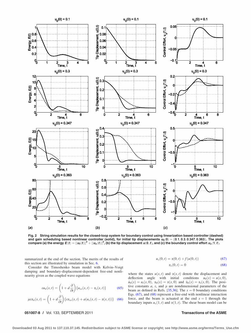
Figure 2 compares the “energy” EðtÞ ¼ jjutðtÞjj2 þ jjuxðtÞjj2, tipdisplacement uð0; tÞ, and boundary control effort uxð1; tÞ of theclosed-loop system for the linearization based controller and thegain scheduling based nonlinear controller. The string is initial-ized with zero initial velocity and the initial displacement profileu0ðxÞ ¼ u0ð0Þ 1� xð Þ for the initial tip displacementsu0ð0Þ ¼ 0:1; 0:3; 0:347; 0:363f g. For sufficiently small initialconditions u0ð0Þ ¼ 0:1ð Þ, which lie in the linear region of theinteraction force, both cases perform equally well. For intermedi-ate initial conditions u0ð0Þ ¼ 0:3ð Þ both cases stabilize the stringwith the gain scheduling based nonlinear controller achieving animproved transient response and slightly quicker settling time.When u0ð0Þ ¼ 0:347, which is the largest initial condition forwhich the linearization based controller stabilizes the origin, thegain scheduling based nonlinear controller clearly outperforms thelinearization based controller in both transient response and set-tling time. When u0ð0Þ ¼ 0:363, which is the largest initial condi-tion for which the gain scheduling based nonlinear controller sta-bilizes the origin, the linearization based controller can no longerstabilize the origin while the gain scheduling based nonlinear con-troller must work hard to keep the nonlinearity from pulling thetip away from the origin. The simulations show that—for a nonli-nearity where the linearization underestimates the force—the gainscheduled based nonlinear controller outperforms the linearizationbased controller when the tip begins to operate in a sufficientlystrong region of the nonlinear interaction force. The transientenergy of the closed-loop system with gain scheduling based non-linear control tends to be higher because of the increased controleffort required for improved performance.

Figure 3 compares the performance of the linearization basedcontroller and gain scheduling based nonlinear controller, whenthe goal is to generate and track the reference trajectoryurð0; tÞ ¼ 0:3 sin pt. The string is initialized with zero initial con-ditions. The gain scheduling based nonlinear controller is able togenerate and track the sinusoid, with a small negative error inthe mean. The negative error in the mean is caused by uð0; tÞinteracting most with the nonlinearity through a negative peakof the sinusoid first. This is confirmed by simulations withurð0; tÞ ¼ �0:3 sin pt where the tip displacement interacts mostwith the nonlinearity through a positive peak of the sinusoid first,and the resulting error in the mean is positive. The negative meancauses a stronger interaction force for the negative peaks, whichin turn causes phase tracking errors between them and the positivepeaks. Conversely, the negative mean causes a weaker interactionforce for the positive peaks, which allows for better tracking frompositive to negative peaks. The plot also shows how the lineariza-tion based controller begins to generate and track the referencetrajectory with the same error in the mean, but ultimately cannotcompensate for the destabilizing force caused by increased inter-action with the negative peaks. As with the stabilization simula-tions, the controllers have comparable performance for smallreference amplitudes and the gain scheduled controller outper-forms the linearization based controller when the amplitudeincreases, and neither controller can stabilize the reference trajec-tory when the reference amplitude is too large.

5 Application to the Shear Beam PDE

This section presents only the application of the gain schedulingbased PDE backstepping techniques of Sec. 2 to the control designfor the shear beam with Kelvin–Voigt damping and boundary-dis-placement-dependent free-end nonlinearity. No theoretical resultsor stability analysis for a closed-loop system are presented here,but they can be pursued using the tools developed in Sec. 2.1.Conditions under which the results of this section would holdlocally, proposed based on the results of Theorem 2.1, are

Fig. 1 Comparison of the nonlinearity f uð0; tÞð Þ used in thestring simulations, and its linear approximation f 0ð0Þuð0; tÞ.

Journal of Dynamic Systems, Measurement, and Control SEPTEMBER 2011, Vol. 133 / 051007-7

Downloaded 03 Aug 2011 to 137.110.37.145. Redistribution subject to ASME license or copyright; see http://www.asme.org/terms/Terms_Use.cfm

summarized at the end of the section. The merits of the results ofthis section are illustrated by simulation in Sec. 6.

Consider the Timoshenko beam model with Kelvin–Voigtdamping and boundary-displacement-dependent free-end nonli-nearity given as the coupled wave equations

euttðx; tÞ ¼ 1þ d@

@t

� �uxxðx; tÞ � axðx; tÞf g (65)

leattðx; tÞ ¼ 1þ d@

@t

� �eaxxðx; tÞ þ a uxðx; tÞ � aðx; tÞð Þf g (66)

uxð0; tÞ ¼ að0; tÞ þ f u 0; tð Þð Þ (67)

axð0; tÞ ¼ 0 (68)

where the states uðx; tÞ and aðx; tÞ denote the displacement anddeflection angle with initial conditions u0ðxÞ ¼ uðx; 0Þ,_u0ðxÞ ¼ utðx; 0Þ, a0ðxÞ ¼ aðx; 0Þ and _a0ðxÞ ¼ atðx; 0Þ. The posi-tive constants a, e, and l are nondimensional parameters of thebeam as defined in Refs. [35,36]. The x ¼ 0 boundary conditionsEqs. (67), and (68) represent a free-end with nonlinear interactionforce, and the beam is actuated at the end x ¼ 1 through theboundary inputs uxð1; tÞ and að1; tÞ. The shear beam model can be

Fig. 2 String simulation results for the closed-loop system for boundary control using linearization based controller (dashed)and gain scheduling based nonlinear controller (solid), for initial tip displacements u0ð0Þ ¼ 0:1;0:3;0:347; 0:363f g. The plotscompare (a) the energy EðtÞ ¼ jjut ðtÞjj2 þ jjux ðtÞjj2, (b) the tip displacement uð0; tÞ, and (c) the boundary control effort ux ð1; tÞ.

051007-8 / Vol. 133, SEPTEMBER 2011 Transactions of the ASME

Downloaded 03 Aug 2011 to 137.110.37.145. Redistribution subject to ASME license or copyright; see http://www.asme.org/terms/Terms_Use.cfm

written as a singular perturbation ðl ¼ 0Þ of the Timoshenkobeam model, and is given by

euttðx; tÞ ¼ 1þ d@

@t

� �uxxðx; tÞ � axðx; tÞf g (69)

0 ¼ eaxxðx; tÞ þ a uxðx; tÞ � aðx; tÞð Þ (70)

with boundary conditions (67) and (68) and boundary inputsuxð1; tÞ, að1; tÞ. As with the string, f ð�Þ is considered to be destabi-lizing, and a gain scheduling based PDE backstepping design ischosen to stabilize u � 0, a � 0.

The results in Ref. [31, Sec. 3] are for an undamped ðd ¼ 0Þshear beam with linear destabilizing force, i.e., constant �f . Thepresence of KV damping in this problem does not change thedesign, and the gain scheduling based backstepping transforma-tions are Eqs. (2) and (3), where for the present problem with�f ðuð0; tÞÞ the boundary-displacement-dependent gains satisfy thepartial integro-differential equations

kxx x; y; uð0; tÞð Þ ¼ kyy x; y; uð0; tÞð Þ þ b2k x; y; uð0; tÞð Þ

þ b3

ðx

y

k x; n; uð0; tÞð Þ sinh b n� yð Þð Þ dn

� b3 sinh b x� yð Þð Þ(71)

k x; x; uð0; tÞð Þ ¼ � b2

2xþ �f uð0; tÞð Þ � c0 (72)

ky x; 0; uð0; tÞð Þ ¼ �b2 cosh bxð Þ þ b2

ðx

0

k x; y; uð0; tÞð Þ cosh byð Þ dy

þ �f uð0; tÞð Þk x; 0; uð0; tÞð Þ(73)

and

lxx x; y;wð0; tÞð Þ ¼ lyy x; y;wð0; tÞð Þ � b2l x; y;wð0; tÞð Þ

� b3

ðx

y

l x; n;wð0; tÞð Þ sinh b n� yð Þð Þ dn

� b3 sinh b x� yð Þð Þ(74)

l x; x;wð0; tÞð Þ ¼ � b2

2xþ �f wð0; tÞð Þ � c0 (75)

ly x; 0;wð0; tÞð Þ ¼ �b2 cosh bxð Þ þ c0l x; 0;wð0; tÞð Þ (76)

Here Eqs. (71)–(73) were found by substituting �q � �f ð�Þ in Eq.(3.9), of Ref. [31], while Eqs. (74)–(76) were found using gainscheduling based PDE backstepping techniques. Note that Eqs.(71)–(73), Eqs. (74)–(76) are families of PIDEs in independentvariables ðx; yÞ, and parametrized by uð0; tÞ, wð0; tÞ. For eachmeasured uð0; tÞ, wð0; tÞ the PIDEs are solved and their solutionssubstituted appropriately. Given that kðx; y; uð0; tÞÞ andlðx; y;wð0; tÞÞ are implemented ‘continuously,’ then an alternativeto numerically solving their respective PIDEs is to approximatethe functions by the explicit first step of a symbolic recursion[31]. The first step of the recursion for the shear beam gainsgives k0 x; y; uð0; tÞð Þ ¼ Pðx; y; uð0; tÞÞ and l0 x; y;wð0; tÞð Þ¼ Pðx; y;wð0; tÞÞ, where Pðx; y; nÞ ¼ �ðb=2Þ � sinh bðx� yÞð Þþ½by cosh bðx� yÞð Þ� þ �f nð Þ � c0. Similar to Ref. [31, Sec. 3] thelocally stabilizing boundary controllers are chosen as

uxð1; tÞ ¼ k 1; 1; uð0; tÞð Þuð1; tÞ þð1

0

kx 1; y; uð0; tÞð Þuðy; tÞ dy

� c1utð1; tÞ þ c1

ð1

0

k 1; y; uð0; tÞð Þutðy; tÞ dy

(77)

að1; tÞ ¼ b sinhðbÞuð0; tÞ � b2

ð1

0

cosh bð1� yÞð Þuðy; tÞ dy (78)

The boundary controller Eq. (77) was found by making substitu-tions, similar to those made for the string, into Eq. 3.7 of Ref. [31]while Eq. (78) is carried over from Refs. [31–34]. Numericalresults in Ref. [34] show comparable performance of the boundarycontrollers when applied with the first step approximationk0 x; y; uð0; tÞð Þ or with the numerical solution of Eqs. (71)–(73)Similar to the string, when �f is constant the closed-loop systemEqs. (67)–(78) is equivalent to the exponentially stable target sys-tem Eqs. (50)–(52), and for general �f ð�Þ the target system is Eqs.(51)–(53) with lðx; y;wð0; tÞÞ given by the numerical solution ofEqs. (74)–(76), or approximated by l0 x; y;wð0; tÞð Þ.

The motion planning and tracking results of Refs. [29,30] canalso be extended to Eqs. (67)–(70) using gain scheduling techni-ques. As with the string, previous motion planning and trackingresults were developed only for �f � 0. Results for general �f ð�Þ arefound following the techniques in Refs. [29,30] but with the trans-formations Eqs. (2), (3), (71)–(73), and (74)–(76) The gain sched-uling based backstepping transformations for motion planning andtracking are

wðx; tÞ ¼ uðx; tÞ þ rðx; tÞ �ðx

0

kðx; y; uð0; tÞÞuðy; tÞ dy (79)

uðx; tÞ ¼ wðx; tÞ � rðx; tÞ þðx

0

lðx; y;wð0; tÞÞ wðy; tÞ � rðy; tÞ½ � dy

(80)

where kðx; y; uð0; tÞÞ and lðx; y;wð0; tÞÞ are given by Eqs. (71)–(73) and (74)–(76), and rðx; tÞ is the state of an auxiliary systemgoverned by a second-order parabolic PDE forced by arð0; tÞ. Themotion planning reference solutions are

urðx; tÞ ¼ wrðx; tÞ � rðx; tÞ

þðx

0

l x; y;wrð0; tÞð Þ wrðy; tÞ � rðy; tÞ½ � dy (81)

arðx; tÞ ¼ coshðbxÞarð0; tÞ þ b sinhðbxÞurð0; tÞ

� b2

ðx

0

cosh bðx� yÞð Þurðy; tÞ dy (82)

where for the tip displacement and deflection angle reference tra-jectories Eq. (57) and

Fig. 3 String simulation results comparing the tip displace-ment uð0; tÞ and reference trajectory ur ð0; tÞ when boundarycontrol is applied with linearization based control and gainscheduling based nonlinear control.

Journal of Dynamic Systems, Measurement, and Control SEPTEMBER 2011, Vol. 133 / 051007-9

Downloaded 03 Aug 2011 to 137.110.37.145. Redistribution subject to ASME license or copyright; see http://www.asme.org/terms/Terms_Use.cfm

arð0; tÞ ¼ Aa sin xatð Þ (83)

wrðx; tÞ is given by Eq. (58), and rðx; tÞ is

rðx; tÞ ¼ Aa f1ðxÞ �ðx

0

f1ðx� yÞ/ðyÞ dy

� �sinðxatÞ

þ Aa f2ðxÞ �ðx

0

f2ðx� yÞ/ðyÞ dy

� �cosðxatÞ (84)

with

f1ðxÞ ¼ cðxaÞ sin bðxaÞxð Þ coshðbðxaÞxÞþ cðxaÞ cos bðxaÞxð Þ sinhðbðxaÞxÞ (85)

f2ðxÞ ¼ �cðxaÞ cos bðxaÞxð Þ sinhðbðxaÞxÞþ cðxaÞ sin bðxaÞxð Þ coshðbðxaÞxÞ (86)

/ðxÞ ¼ �b sinhðbxÞ þ b

ðx

0

k x; y; uð0; tÞð Þ sinhðbyÞ dy (87)

where bðxaÞ, bðxaÞ, cðxaÞ, cðxaÞ are given in Eqs. (59)–(62) Theboundary inputs for motion planning are

urxð1; tÞ ¼ wr

xð1; tÞ � rxð1; tÞ þ l 1; 1;wrð0; tÞð Þ wrð1; tÞ � rð1; tÞ½ �

þð1

0

lx 1; y;wrð0; tÞð Þ wrðy; tÞ � rðy; tÞ½ � dy

(88)

arð1; tÞ ¼ coshðbÞarð0; tÞ þ b sinhðbÞurð0; tÞ

� b2

ð1

0

cosh bð1� yÞð Þurðy; tÞ dy (89)

and the tracking boundary controllers are

uxð1; tÞ ¼ k 1; 1; uð0; tÞð Þuð1; tÞ þð1

0

kx 1; y; uð0; tÞð Þuðy; tÞ dy

� c1utð1; tÞ þ c1

ð1

0

k 1; y; uð0; tÞð Þutðy; tÞ dyþ wrxð1; tÞ

þ c1wrt ð1; tÞ � rxð1; tÞ � c1rtð1; tÞ

(90)

að1; tÞ ¼ coshðbÞarð0; tÞ þ b sinhðbÞuð0; tÞ

� b2

ð1

0

cosh bð1� yÞð Þuðy; tÞ dy (91)

The beam boundary controllers (77), (78) and (90), (91) requireactuation of the slope (or displacement) and bending moment atthe base. When combined with full state observers [31–34], theoutput-feedback controllers require sensing of the free-end dis-placement and velocity.

Based on the results of Theorem 2.1, the initial conditionsu0ðxÞ, _u0ðxÞ, u0ðxÞ � ur

0ðxÞ, and _u0ðxÞ � _ur0ðxÞ, along with the ref-

erence trajectory urð0; tÞ should be sufficiently small in the appro-priate norms for the nonlinear controllers Eqs. (77), (78) and (90),(91) to be exponentially stabilizing and for the reference solutionsEqs. (81) and (82) to hold. Such restrictions would seem to con-fine the operation to a linear region of f ð�Þ. Since the advantage ofusing the nonlinear gain scheduled controls is impossible to quan-tify using the conservative analysis tools of Sec. 2.1, then theadvantage of gain scheduling based control over linearizationbased control is illustrated by simulations in Sec. 6.

6 Simulations for the Timoshenko Beam

The Timoshenko beam control design in Refs. [33,34] is doneusing a singular perturbation approach to reduce it to the shearbeam model, with the rest of the design being analogous to the

shear beam results in Refs. [31,32]. All results for the shear beamapply approximately to the Timoshenko beam, therefore the gainscheduling based designs for the shear beam also apply approxi-mately to the Timoshenko beam.

Simulations are done for the Timoshenko beam Eqs. (65)–(68)with the stabilizing boundary controllers Eqs. (77) and (78) andtracking controllers Eqs. (90) and (91) using the numerical solu-tion to the gain PIDE, Eqs. (71)–(73) The spatial and temporalstep sizes are Dx ¼ 1

100and Dt ¼ 1

50, respectively, the beam param-

eters are a ¼ 5, d ¼ 0:1, e ¼ 10, and l ¼ 0:02, and the controllerparameters are c0 ¼ 10 and c1 ¼ 0:99

ffiffiffiffiffi10p

. String simulationswere done with a superlinear nonlinearity which demanded amore aggressive control action. Beam simulations are done with asublinear nonlinearity which demands a less aggressive controlaction. Figure 4 compares the nonlinearity f uð0; tÞð Þ ¼ �Fuð0; tÞ=1þ 3uð0; tÞð Þ2 for F ¼ 1, where F is the linear strength of theforce, and its linear approximation about the origin. The bound-ary-displacement-dependent interaction force has a linear regionabout the origin, which is then dominated by the quadratic nonli-nearity in the denominator. The linear approximation overesti-mates the interaction force, i.e. jf 0ð0Þuð0; tÞj � jf uð0; tÞð Þj for alluð0; tÞ. This sublinear nonlinearity is easier to compensate forcompared to superlinear nonlinearity used for the string since,though it may destabilize the origin, its strength decreases farfrom the origin and it can add two new stable equilibria atuð0; tÞj j > 0.

Figure 5 compares the energy EðtÞ, tip displacement uð0; tÞ, andboundary control effort uxð1; tÞ of the closed-loop system for thelinearization based controller and the gain scheduling based non-linear controller. The beam is initialized with zero initial velocityand the initial displacement and deflection angle profilesu0ðxÞ ¼ 3

101� xð Þ2 and a0ðxÞ ¼ � 3

51� xð Þ, and the nonlinearity

strength is varied as F ¼ f0:1; 0:3; 0:53; 2; 2:8g. The goal ofthese simulations is to compare the two control implementations,as opposed to finding the best control parameters c0 and c1 for aparticular F, therefore the same c0 and c1 were used for all valuesof F. For a very weak force ðF ¼ 0:1, not shown), the controllershave similar performance. As the strength of the force increasesðF ¼ 0:3 to F ¼ 0:53Þ the nonlinear controller consistently per-forms well. Conversely, performance of the linearization basedcontroller begins to degrade as the overestimating nature of thegain induces oscillation and the origin transitions from stable, tomarginally stable, to unstable. For a strong force ðF ¼ 2Þ the non-linear controller is still able to stabilize the origin. The gain sched-uled controller extends the range of stability to F ¼ 2:8 (notshown), which is the largest value for which the nonlinear control-ler (with c0 ¼ 10Þ preserves stability of the origin. Simulationswith F ¼ 2:8 show that increasing the value of c0 improves per-formance, suggesting that c0 should be increased proportional toF, though ultimately the gain scheduling based nonlinear control-ler cannot stabilize the origin for very large F. The simulations

Fig. 4 Comparison of the nonlinearity f uð0; tÞð Þ used for thebeam simulations, and its linear approximation f 0ð0Þuð0; tÞ, forF ¼ 1.

051007-10 / Vol. 133, SEPTEMBER 2011 Transactions of the ASME

Downloaded 03 Aug 2011 to 137.110.37.145. Redistribution subject to ASME license or copyright; see http://www.asme.org/terms/Terms_Use.cfm

show that—for a nonlinearity where the linearization overesti-mates the force—the nonlinear controller outperforms the lineari-zation based controller when the nonlinear interaction forcebecomes sufficiently strong, and it extends the range of stability.

Figure 6 compares the performance of the linearization basedcontroller and gain scheduling based nonlinear controller whenthe goal is to generate and track the reference trajectoryurð0; tÞ ¼ 0:5 sin pt=3ð Þ, arð0; tÞ ¼ 0. The beam is initialized withzero initial conditions. The plot shows how the linearization basedcontroller begins to generate the reference trajectory, but in over-estimating the nonlinearity it applies an excess of control effortproducing large amplitude and phase errors, and cannot compen-sate for the harmonics caused by interaction with the nonlinearity.The linearization based controller eventually destabilizes the sys-tem for larger time. The gain scheduling based nonlinear control-ler is able to generate and track the sinusoid with very small errorsin amplitude and phase, part of which can be attributed to the ap-proximate nature of the shear beam results applied to the Timo-shenko beam [29,30]. The controllers have comparable perform-ance for small reference amplitudes and force strengths, the gainscheduled controller outperforms the linearization based control-ler when the reference amplitude or force strength increases, andneither controller can stabilize the reference trajectory when thestrength of the force is too large.

Fig. 5 Beam simulation results showing the closed-loop system with linearization based control (dashed) and gain schedul-ing based nonlinear control (solid). The beam is initialized with u0ðxÞ ¼ 3

10 1� xð Þ2 and a0ðxÞ ¼ � 35 1� xð Þ and zero velocities,

and the nonlinearity strength is varied as F ¼ f0:3; 0:53;2g. The plots compare the (a) energy EðtÞ, (b) tip displacement uð0; tÞ,and (c) boundary control effort ux ð1; tÞ.

Fig. 6 Beam simulation results comparing the tip displace-ment and reference trajectory when boundary control is appliedwith linearization based control and gain scheduling basednonlinear control.

Journal of Dynamic Systems, Measurement, and Control SEPTEMBER 2011, Vol. 133 / 051007-11

Downloaded 03 Aug 2011 to 137.110.37.145. Redistribution subject to ASME license or copyright; see http://www.asme.org/terms/Terms_Use.cfm

7 Conclusions

A control design for nonlinear PDEs inspired by gain schedul-ing and based on the backstepping theory for linear PDEs hasbeen introduced. Control designs were presented for a benchmarkfirst-order hyperbolic PDE with boundary-value-dependent in-do-main nonlinearity, and for the string and shear beam with Kelvin–Voigt damping and boundary-displacement-dependent free-endnonlinearities. The benchmark system was used to illustrate howone can perform a stability analysis of a nonlinear PDE systemwith gain scheduling based nonlinear control. Stability analysisshowed that the equilibrium u � 0 of the closed-loop system waslocally exponentially stable. String and Timoshenko beam simula-tions were presented to show the performance of the gain schedul-ing based nonlinear controllers, which outperformed simple linea-rization based controllers.

Gain scheduling based PDE boundary backstepping methodsprovide a simple and effective solution to the difficult problem ofnonlinear control design for infinite dimensional nonlinear sys-tems. While not as powerful as a full nonlinear design, gain sched-uling based PDE backstepping theory produces tractable resultsthat outperform simple linearization based design.

Acknowledgment

This research was supported by the Los Alamos National Labo-ratory and the National Science Foundation.

References[1] Boskovic, D., and Krstic, M., 2001, “Nonlinear Stabilization of a Thermal Con-

vection Loop by State Feedback,” Automatica, 37, pp. 2033–2040.[2] Boskovic, D., and Krstic, M., 2002, “Backstepping Control of Chemical Tubu-

lar Reactors,” Comput. Chem. Eng., 26, pp. 1077–1085.[3] Boskovic, D., and Krstic, M., 2003, “Stabilization of a Solid Propellant Rocket

Instability by State Feedback,” Int. J. Robust Nonlinear Control, 13, pp. 483–495.[4] Armaou, A., and Christofides, P. D., 2000, “Wave Suppression by Nonlinear

Finite-Dimensional Control,” Comput. Chem. Eng., 55(14), pp. 2627–2640.[5] Armaou, A., 2004, “Output Feedback Control of Dissipative Distributed Proc-

esses Via Microscopic Simulations,” Comput. Chem. Eng., 29(4), pp. 771–782.[6] Varshney, A., Pitchaiah, S., and Armaou, A., 2009, “Feedback Control of Dissi-

pative PDE Systems Using Adaptive Model Reduction,” AIChE J., 55(4), pp.906–918.

[7] Christofides, P. D., 2001, Nonlinear and Robust Control of PDE Systems: Meth-ods and Applications to Transport-Reaction Processes, Birkhauser, Boston,MA.

[8] Kugi, A., Thull, D., and Kuhnen, K., 2006, “An Infinite-Dimensional ControlConcept for Piezoelectric Structures With Complex Hysteresis,” Struct. ControlHealth Monit., 13, pp. 1099–1119.

[9] Meurer, T., and Zeitz, M., 2005, “Feedforward and Feedback Tracking Controlof Nonlinear Diffusion-Convection-Reaction Systems Using SummabilityMethods,” Ind. Eng. Chem. Res., 44, pp. 2532–2548.

[10] Banach, A. S., and Baumann, W. T., 1990, “Gain-Scheduled Control of Nonlin-ear Partial Differential Equations,” Proceedings of the Conference on Decisionand Control, pp. 387–392.

[11] Vazquez, R., and Krstic, M., 2008, “Control of 1-D Parabolic PDEs With Vol-terra Nonlinearities—Part I: Design,” Automatica, 44, pp. 2778–2790.

[12] Vazquez, R., and Krstic, M., 2008, “Control of 1-D Parabolic PDEs With Vol-terra Nonlinearities—Part II: Analysis,” Automatica, 44, pp. 2791–2803.

[13] Cloutier, J. R., 1997, “State-Depedent Riccati Equation Techniques: An Over-view,” Proceedings of the American Control Conference, pp. 932–936.

[14] Cloutier, J. R., and Stansbery, D. T., 1999, “Control of a Continuously StirredTank Reactor Using an Asymmetric Solution of the State-Dependent Riccatiequation,” Proceedings of the IEEE International Conference on Control Appli-cations, pp. 893–898.

[15] Cloutier, J. R., and Stansbery, D. T., 2002, “The Capabilities and Art of State-Dependent Riccati Equation-Based Design,” Proceedings of the American Con-trol Conference, pp. 86–91.

[16] Khalil, H. K., 2002, Nonlinear Systems, 3rd ed., Prentice Hall, Upper SaddleRiver, NJ.

[17] Rugh, W. J., 1990, “Analytical Framework for Gain Scheduling,” Proceedingsof the American Control Conference, pp. 79–84.

[18] Rugh, W. J., and Shamma, J. S., 2000, “Research on Gain Scheduling,” Auto-matica, 36, pp. 1401–1425.

[19] Shamma, J. S., and Athans, M., 1990, “Analysis of Gain Scheduled Control forNonlinear Plants,” IEEE Trans. Autom. Control, 35(8), pp. 898–907.

[20] Shamma, J. S., and Athans, M., 1991. “Gain Scheduling: Potential Hazards andPossible Remedies,” Proceedings of the American Control Conference, pp.101–107.

[21] Shamma, J. S., and Athans, M., 1991, “Guaranteed Properties of Gain Sched-uled Control for Linear Parameter-Varying Plants,” Automatica, 27(3), pp.559–564.

[22] Shamma, J. S., and Cloutier, J. R., 2003, “Existence of SDRE StabilizingFeedback,” IEEE Trans. Autom. Control, 48, pp. 513–517.

[23] Wang, J., and Rugh, W. J., 1987, “Feedback Linearization Families for Nonlin-ear Systems,” IEEE Trans. Autom. Control, 32(10), pp. 935–940.

[24] Wang, J., and Rugh, W.J., 1987, “Parameterized Linear Systems and Lineariza-tion Families for Nonlinear Systems,” IEEE Trans. Circuits Syst., 34(6), pp.650–657.

[25] Krstic, M., and Smyshlyaev, A., 2008, Boundary Control of PDEs: A Courseon Backstepping Designs, SIAM, Philadelphia, PA.

[26] Krstic, M., and Smyshlyaev, A., 2008, “Backstepping Boundary Control forFirst-Order Hyperbolic PDEs and Application to Systems With Actuator andSensor Delays,” Syst. Control Lett., 57, pp. 750–758.

[27] Krstic, M., Guo, B.-Z., Balogh, A., and Smyshlyaev, A., 2008, “Output-Feed-back Stabilization of an Unstable Wave Equation,” Automatica, 44, pp. 63–74.

[28] Krstic, M., Siranosian, A. A., Balogh, A., and Guo, B.-Z., 2007, “Control ofStrings and Flexible Beams by Backstepping Boundary Control,” Proceedingsof the American Control Conference.

[29] Siranosian, A. A., Krstic, M., Smyshlyaev, A., and Bement, M., 2008, “MotionPlanning and Tracking for Tip displacement and Deflection Angle for FlexibleBeams,” Proceedings of the American Control Conference.

[30] Siranosian, A. A., Krstic, M., Smyshlyaev, A., and Bement, M., 2009, “MotionPlanning and Tracking for Tip Displacement and Deflection Angle for FlexibleBeams,” ASME J. Dyn.Syst., Meas., Control, 131, p. 031009.

[31] Krstic, M., Guo, B.-Z., Balogh, A., and Smyshlyaev, A., 2008, “Control of aTip-Force Destabilized Shear Beam by Observer-Based Boundary Feedback,”SIAM J. Control Optim., 47, pp. 553–574.

[32] Krstic,M., and Balogh, A., 2006, “Backstepping Boundary Controller and Ob-server for the Undamped Shear Beam,” 17th International Symposium on Math-ematical Theory of Networks and Systems.

[33] Krstic, M., Siranosian, A. A., and Smyshlyaev, A., 2006, “Backstepping Bound-ary Controllers and Observers for the Slender Timoshenko beam: Part I—Design,” Proceedings of the American Control Conference.

[34] Krstic, M., Siranosian, A. A., Smyshlyaev, A., and Bement, M., 2006,“Backstepping Boundary Controllers and Observers for the Slender Timo-shenko beam: Part II—Stability and Simulations,” Proceedings of the IEEEConference on Decision and Control.

[35] Han, S. M., Benaroya, H., and Wei, T., 1999, “Dynamics of TransverselyVibrating Beams using four engineering theories,” J. Sound Vib., 225, pp.935–988.

[36] Zhao, H. L., Liu, K. S., and Zhang, C. G., 2004, “Stability for the TimoshenkoBeam System With Local Kelvin–Voigt damping,” Acta Math. Sin. EnglishSer., 21(3), pp. 655–666.

051007-12 / Vol. 133, SEPTEMBER 2011 Transactions of the ASME

Downloaded 03 Aug 2011 to 137.110.37.145. Redistribution subject to ASME license or copyright; see http://www.asme.org/terms/Terms_Use.cfm