Gagnon $6 Trillion

8/14/2019 Gagnon $6 Trillion

http://slidepdf.com/reader/full/gagnon-6-trillion 1/38

The World Needs Further Monetary Ease, Not an Early Exit

Joseph E. Gagnon1

Peterson Institute for International Economics

December 2009

Introduction and Summary

Governments and central banks around the world eased macroeconomic

policies aggressively in response to the 2008 financial crisis, arguably forestalling a

second Great Depression. More recently, however, policymakers have been talking

about when to withdraw the stimulus. This focus on exit is misguided. Current

forecasts show an extended period of economic stagnation in the developed world.

We need additional stimulus now. In particular, central banks in the main

developed economies should push long-term interest rates 75 basis points below the

levels they would otherwise take by purchasing a combined $6 trillion in long-term

public and private debt securities. Relative to current forecasts, this policy action is

expected to boost GDP 3 percent or more over the next eight quarters and to reduce

unemployment rates by between 1 and 3 percentage points.

Without additional stimulus, unemployment rates are likely to remain above

equilibrium levels for many years at great cost to the world economy in terms of lost

income and personal hardship. Moreover, with inflation rates already below desired

levels, excess unemployment threatens to cause an unwelcome fall in prices that

would further damp recovery and retard the necessary process of deleveraging.

In light of high and rising levels of public debt, additional monetary stimulus

1 I would like to thank Fred Bergsten, Tim Duy, Karen Dynan, Marc Hinterschweiger, Jacob

Kirkegaard, Michael Mussa, Adam Posen, David Reifschneider, Howard Rosen, Ted Truman, and

Angel Ubide for helpful advice and comments.



- 2 -

is preferable to additional fiscal stimulus. Indeed, monetary stimulus reduces the

ratio of public debt to GDP by reducing interest expenses, increasing GDP,

expanding tax revenues, and enabling an earlier start to fiscal consolidation.

The following specific actions in the near term would help set the world on a

solid recovery with stable prices and a return of economic activity to its trend

growth path by the end of 2011:

• The Federal Reserve should purchase an additional $2 trillion of longer-term

debt securities, with an average maturity of around 7 years.

• The European Central Bank should lower its main refinancing rate to 50

basis points, continue to extend unlimited 12-month credit to the banking

system at this rate, and purchase €1 trillion of longer-term debt securities.

• The Bank of Japan should state more clearly its intention to return inflation

to at least 1 percent over the next two years, purchase an additional ¥100

trillion of longer-term debt securities with an average maturity of around 7

years, and commit to a further ¥100 trillion in such purchases in 2011 if core

inflation over the next 12 months remains negative.

• The Bank of England should purchase an additional £200 billion of longer-

term sterling bonds or an equivalent amount of longer-term foreign-currency

bonds with the interest and principal hedged using currency swaps.

Renewed asset price bubbles and financial market excesses are unlikely in the

current circumstances, but policymakers must be ready to use supervisory and

regulatory tools to combat risky financial activities should they occur.



- 3 -

Do We Need More Macroeconomic Stimulus?

It is widely agreed that the four main developed economies—the United

States, the euro area, Japan, and the United Kingdom—currently are experiencing

considerable economic slack and rates of inflation below the levels desired by their

central banks. However, because macroeconomic policies operate only with a

substantial lag, there is little that can be done to improve conditions in the

immediate future. Rather, the policy choice today must be made with an eye to

likely conditions beyond the next few months.

Studies typically find that the peak effect of monetary policy on economic

growth occurs after one year and the peak effect of monetary policy on inflation

occurs after two years.2 Fiscal policies typically have a somewhat faster effect on

the economy, but getting them through the legislative and executive hurdles to

implementation takes time.3 Overall, the stance of monetary and fiscal policies

should be aimed at returning economic activity (GDP) reasonably close to its

maximum sustainable level within two years and returning inflation close to its

desired level over two to three years.4 There are times when these two goals may be

in conflict and policy must compromise between them, but such is not the case at

present.

2 See the forthcoming chapter for the Handbook of Monetary Economics by Boivin, Kiley, and

Mishkin (2009). In terms of the level of GDP, the effect peaks around one to two years before dying

out with the effect on employment peaking around, or just over, two years. In terms of the level of

prices, the effect is permanent and largely completed after three years. 3 It is possible to design a fiscal policy with a nearly immediate effect on the economy after it is

implemented (for example, a one-time cash transfer), but most fiscal policies have a more gradual

effect.4 A number of central banks generally aim to achieve their inflation targets within a horizon of two

years, including the Bank of England, the Bank of Canada, and the Swedish Riksbank.



- 4 -

Recent forecasts by private-sector economists, government and international

agencies, and central banks generally project years of lackluster growth and excess

unemployment, with inflation rates that are at or below desired levels. Most of

these forecasts assume that the current stance of monetary and fiscal policy will be

tightened only gradually. The projections of prolonged economic stagnation thus

strongly suggest that the current stance of policies is too tight.

Moreover, the cost of allowing unemployment to remain high is even greater

than lost income and personal hardships in the next few years. Economic research

shows that high levels of unemployment erode worker skills and employability,

which causes an economy’s structural rate of unemployment to rise.5 Getting back

to the initial level of structural unemployment can take decades, with

commensurate losses in economic output, not to mention social distress.

A common theme of most forecasts is that inflation--which currently is below

the levels targeted by central banks--will rise over the next two to three years.

Such projections are not consistent with the standard accelerationist model, which

predicts falling inflation rates as long as the GDP gap is negative and/or excess

unemployment is positive. The Organization for Economic Cooperation and

Development (OECD) attributes the projected rise of inflation to its view that

inflation expectations are well-anchored at central bank target levels and that

“speed-limit” effects push up prices when GDP grows faster than potential.6

However, in each of these economies, all previous occurrences of large negative GDP

5 See Blanchard and Summers (1986) and Ball (2009).6 See OECD (2009, p.65).



- 5 -

gaps since 1970 (using OECD estimates) were associated with declines in rates of

inflation that persisted throughout recoveries that were faster than those projected

for 2010 and 2011; inflation rates subsequently rose only when GDP gaps turned

positive. Given the large magnitude and expected long duration of excess

unemployment, and the relatively modest growth rates projected, it is more

reasonable to expect substantial further declines in rates of inflation.7

Some have argued that economies take longer than normal to return to full

employment after financial crises.8 However, there is a wide range of growth

outcomes after financial crises, and the worst outcomes tended to be associated with

the poorest policy responses.9 The goal of policymakers should be to learn from the

past and achieve a better outcome than simply the average of past outcomes. In the

current crisis, the zero bound on interest rates has been a major factor preventing

monetary policymakers from doing as much as they otherwise would to speed

recoveries. But, as discussed below, the zero bound is not a limit on what monetary

policy can do. There is plenty of scope for further monetary stimulus.

United States

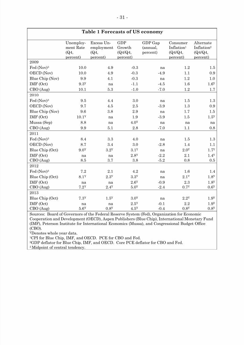
Table 1 presents prominent forecasts of the US economy. Unless otherwise

noted, the GDP growth rate and the inflation rates are four-quarter percent

changes. The unemployment rate is a percent of the labor force. Excess

7 Indeed, in the United States, the four-quarter changes in the employer cost index and hourly

compensation have dropped sharply to levels not seen since World War II, suggesting that inflation

may decline further.8 See Reinhart and Rogoff (2009).9 See IMF (2009). In some cases, such as Japan in the 1990s, the financial crisis may have been

caused or exacerbated by a structural slowdown in economic growth, which would vitiate any

inference about the effect of the financial crisis on economic growth.



- 6 -

unemployment is the difference between the projected unemployment rate and the

forecasting institution’s estimate of the structural or long-run unemployment rate.

The GDP gap is a percent of potential GDP. Except for the GDP gap, and unless

otherwise noted, variables refer to the fourth quarter of each year.

The Blue Chip, Federal Reserve (Fed), OECD, and Congressional Budget

Office (CBO) estimates of long-run unemployment are 5.8 percent, 5.1 percent, 5.0

percent, and 4.8 percent, respectively.10 Based on these estimates, excess

unemployment is currently around 4 to 5½ percent, which is the highest level since

the Great Depression according to the CBO’s historical estimates. All of these

forecasts show excess unemployment continuing to exceed 3 percent of the labor

force at the end of 2011, eight quarters from now, and exceeding 2 percent of the

labor force at the end of 2012. Such a degree and duration of slack in the labor

market has not been witnessed since the Great Depression.11 Even the Mussa

forecast, which is the most optimistic of these forecasts, shows an unemployment

rate at the end of 2010 that is at least three percentage points higher than any of

the estimates of the structural rate of unemployment.

The forecasts generally show modest GDP growth rates in 2010 with some

pick-up in 2011. However, these growth projections are far smaller than the 5

percent average GDP growth that occurred in the three years following each of the

two previous recessions of comparable magnitude: 1974-75 and 1981-82. The GDP

10 The OECD projects that structural unemployment will rise to 5.3 percent by 2011 and then return

to 5.0 percent by 2017.11 Indeed, both CBO and OECD historical estimates show that excess unemployment never exceeded

3 percent in even a single quarter for the 25 years from 1983 to 2008, including the 1990-91 and

2001 recessions.



- 7 -

gaps are projected to remain large by historical standards in 2011. The slowness

with which the GDP gaps are projected to close is particularly striking in light of

the fact that these forecasters project that potential GDP growth has temporarily

slowed in the near term by as much as 1.5 percentage points.

The Blue Chip and International Monetary Fund (IMF) forecasts have

inflation rates quickly rebounding to about the Fed’s desired level of close to 2

percent, whereas the Fed, the OECD and the CBO see persistent shortfalls of

inflation below this level.

Euro Area

Table 2 presents forecasts of the euro area economy. The data refer to

annual averages or year-on-year changes, but are otherwise similar to those

presented for the United States. The unemployment rate is uniformly projected to

increase over the next two years. Excess unemployment also is projected to rise

notably next year. The small drop in excess unemployment in 2011 is entirely

accounted for by the OECD’s projection of an increasing rate of structural

unemployment caused by the increase in actual unemployment, a process also

known as hysteresis. The increase in unemployment since 2008 is smaller than in

the United States, despite a larger decline in GDP, likely reflecting activist

employment policies and subsidies in some of the large euro-area countries. GDP

growth is projected to be lackluster, with the GDP gap declining very little over the

next two years.12 Inflation is projected to remain below the European Central

12 Although the ECB did not publish a GDP gap in its December forecast, it noted that the output

gap is projected to remain “significantly negative” through 2011.



- 9 -

remain high and the GDP gap is projected to remain large through at least 2011.

Notably, the Bank of England (BOE) (which does not publish a GDP gap) projects

much faster GDP growth over the next two years than the other forecasters,

including Mussa, who has the highest GDP forecast for each of the other

economies.13 The BOE publishes two forecasts: one based on market expectations of

rising future policy rates and one based on future short-term policy rates held

constant at their current value of 0.5 percent. Not surprisingly, the forecast

assuming the constant low policy rate projects a higher GDP growth rate and higher

inflation, with inflation rising above target by late 2011. Presumably, the GDP gap

implicit in the BOE-Constant forecast is closed by the end of 2011, which suggests

that the BOE’s estimate of the current GDP gap is smaller than those of other

forecasters or that the BOE has a lower estimate of the potential growth rate than

other forecasters.

If the BOE’s view of the economic outlook is correct, then there is little need

for additional macroeconomic stimulus in the United Kingdom. However, if most

other forecasters are right, then there is a need for substantial additional stimulus.

13 The BOE’s median growth projections are even larger than the mean projections shown here.



- 10 -

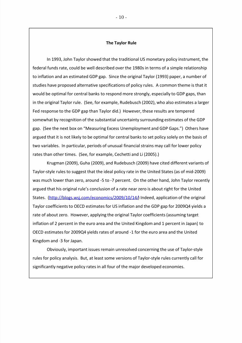
The Taylor Rule

In 1993,

John

Taylor

showed

that

the

traditional

US

monetary

policy

instrument,

the

federal funds rate, could be well described over the 1980s in terms of a simple relationship

to inflation and an estimated GDP gap. Since the original Taylor (1993) paper, a number of

studies have proposed alternative specifications of policy rules. A common theme is that it

would be optimal for central banks to respond more strongly, especially to GDP gaps, than

in the original Taylor rule. (See, for example, Rudebusch (2002), who also estimates a larger

Fed response to the GDP gap than Taylor did.) However, these results are tempered

somewhat by

recognition

of

the

substantial

uncertainty

surrounding

estimates

of

the

GDP

gap. (See the next box on “Measuring Excess Unemployment and GDP Gaps.”) Others have

argued that it is not likely to be optimal for central banks to set policy solely on the basis of

two variables. In particular, periods of unusual financial strains may call for lower policy

rates than other times. (See, for example, Cechetti and Li (2005).)

Krugman (2009), Guha (2009), and Rudebusch (2009) have cited different variants of

Taylor‐style rules to suggest that the ideal policy rate in the United States (as of mid‐2009)

was much

lower

than

zero,

around

‐5 to

‐7 percent.

On

the

other

hand,

John

Taylor

recently

argued that his original rule’s conclusion of a rate near zero is about right for the United

States. (http://blogs.wsj.com/economics/2009/10/14/) Indeed, application of the original

Taylor coefficients to OECD estimates for US inflation and the GDP gap for 2009Q4 yields a

rate of about zero. However, applying the original Taylor coefficients (assuming target

inflation of 2 percent in the euro area and the United Kingdom and 1 percent in Japan) to

OECD estimates for 2009Q4 yields rates of around ‐1 for the euro area and the United

Kingdom and

‐3 for

Japan.

Obviously, important issues remain unresolved concerning the use of Taylor‐style

rules for policy analysis. But, at least some versions of Taylor‐style rules currently call for

significantly negative policy rates in all four of the major developed economies.



- 11 -

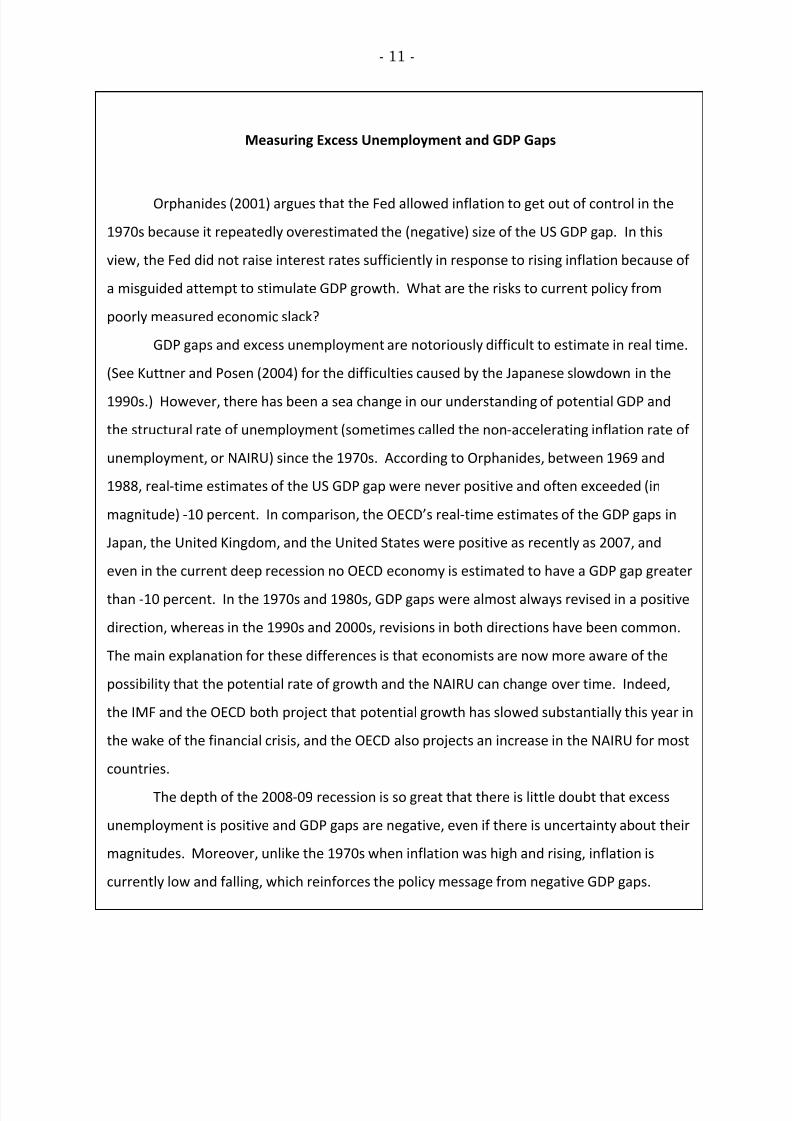
Measuring Excess Unemployment and GDP Gaps

Orphanides (2001)

argues

that

the

Fed

allowed

inflation

to

get

out

of

control

in

the

1970s because it repeatedly overestimated the (negative) size of the US GDP gap. In this

view, the Fed did not raise interest rates sufficiently in response to rising inflation because of

a misguided attempt to stimulate GDP growth. What are the risks to current policy from

poorly measured economic slack?

GDP gaps and excess unemployment are notoriously difficult to estimate in real time.

(See Kuttner and Posen (2004) for the difficulties caused by the Japanese slowdown in the

1990s.) However, there has been a sea change in our understanding of potential GDP and

the structural rate of unemployment (sometimes called the non‐accelerating inflation rate of

unemployment, or NAIRU) since the 1970s. According to Orphanides, between 1969 and

1988, real‐time estimates of the US GDP gap were never positive and often exceeded (in

magnitude) ‐10 percent. In comparison, the OECD’s real‐time estimates of the GDP gaps in

Japan, the United Kingdom, and the United States were positive as recently as 2007, and

even in the current deep recession no OECD economy is estimated to have a GDP gap greater

than ‐10 percent. In the 1970s and 1980s, GDP gaps were almost always revised in a positive

direction, whereas in the 1990s and 2000s, revisions in both directions have been common.

The main explanation for these differences is that economists are now more aware of the

possibility that the potential rate of growth and the NAIRU can change over time. Indeed,

the IMF and the OECD both project that potential growth has slowed substantially this year in

the wake of the financial crisis, and the OECD also projects an increase in the NAIRU for most

countries.

The depth of the 2008‐09 recession is so great that there is little doubt that excess

unemployment is positive and GDP gaps are negative, even if there is uncertainty about their

magnitudes. Moreover, unlike the 1970s when inflation was high and rising, inflation is

currently low and falling, which reinforces the policy message from negative GDP gaps.



- 12 -

Monetary Policy Effectiveness at the Zero Bound

Central banks in the four major developed economies have pushed overnight

interest rates to near-zero levels. They also have employed an array of

nontraditional policies. Most of these policies were aimed at restoring normal

functioning to financial markets and thus tended to offset financial headwinds

rather than provide macroeconomic stimulus beyond that implied by the level of the

policy interest rate. For example, actions by the Fed to support the commercial

paper (CP) market quickly returned the spreads of CP interest rates over Treasury

rates to historically normal levels from unusually elevated levels last fall.

Nevertheless, the lingering effects of financial strains are continuing to curtail some

of the traditional channels of policy stimulus. For example, surveys of bank lending

standards in all four major developed economies show an exceptionally pronounced

tightening of credit standards and terms in 2008 with further tightening (except for

Japan) in 2009.14

These headwinds are a major factor behind the forecasts of a slow

economic recovery.

What More Can Central Banks Do?

One class of policies that can provide additional macroeconomic stimulus

when traditional policy rates are near the zero bound is the large-scale purchase of

long-term government bonds and other liquid long-term assets, which pushes down

interest rates at longer maturities. The BOE and the Fed have purchased

substantial quantities of such assets and these policies have reduced long-term

14 See the Fed’s Senior Loan Officer Opinion Survey on Bank Lending Practices, the ECB’s Euro Area

Bank Lending Survey, the BOJ’s Senior Loan Officer Opinion Survey on Bank Lending Practices at

Large Japanese Banks, and the BOE’s Credit Conditions Survey.



- 13 -

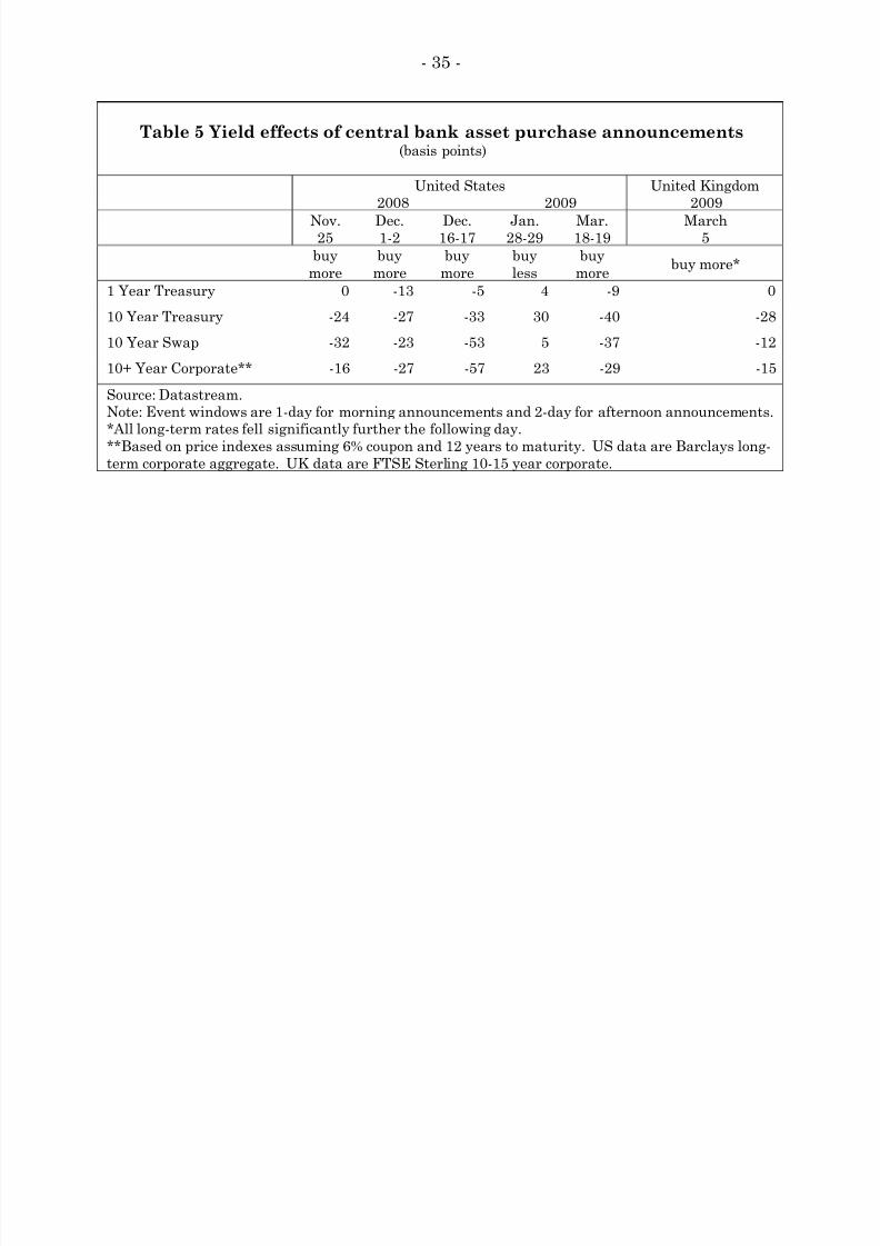
interest rates.15 Table 5 lists the movements in various interest rates over one- and

two-day event windows surrounding Fed and BOE communications about such

asset purchases.16 The movements are always in the expected direction—increased

purchases of long-term assets reduce long-term interest rates. Moreover, the effects

appear to be long-lasting. For example, mortgage rates in the United States—a key

target of the Fed’s purchases—remain more than 1 percentage point lower than

they were in mid-November 2008.17

The cumulative change in the 10-year Treasury yield across the five US

events shown in Table 5 is -94 basis points. If this change were attributed to the

Fed’s announced purchases of $1.75 trillion in longer-term assets, it would imply

that each $1 trillion in such purchases would lower the 10-year yield 54 basis

points. However, it seems likely that market participants initially attached a

significant probability to increases in the amount of Fed purchases beyond $1.75

trillion, because the 10-year yield rose on balance after subsequent Fed

15 The ECB is purchasing €60 billion of covered bonds, which represents a much smaller program

relative to GDP than the BOE and Fed programs. The BOJ has stepped up its purchases of

government bonds significantly, but these purchases have been concentrated at shorter maturities.

See McCauley and Ueda (2009).16 On November 25, 2008 the Fed announced a program to purchase up to $100 billion of agency debt

and $500 billion of agency MBS. On December 1, Chairman Bernanke raised the possibility of

buying longer-term Treasury securities. On December 16 the Fed confirmed the agency program and

reiterated the possibility of buying Treasury securities. On January 28 the Fed disappointedmarkets by not announcing Treasury purchases. On March 18 the Fed announced a Treasury

purchase program of up to $300 billion and expanded the agency MBS program to $1.25 trillion. On

March 5 the BOE announced an asset purchase program of £75 billion, potentially expandable to

£150 billion. Subsequent announcements involved much smaller amounts and were largely

anticipated by markets. Notably, on November 5 the BOE announced a £25 billion increase in its

purchases that was interpreted as the likely final installment, thereby reducing market expectations

of the ultimate scale of the purchase program. Long-term interest rates rose moderately on that day.17 Long-term Treasury yields have risen modestly since late March, but this rise reflects an

unwinding of safe-haven flows, as long-term corporate yields have dropped sharply.



- 14 -

announcements that did not indicate any increase beyond $1.75 trillion.18 The

cumulative yield movement around all Fed announcements concerning asset

purchases is -67 basis points, or -39 basis points per $1 trillion.19 This estimate

must be considered very imprecise, however, because it assumes that all the effects

of the Fed’s actions showed up in market rates within narrow windows of time and

that market participants did not change their views about the Fed purchases (up or

down) outside these windows.

The ability of central banks to drive down long-term interest rates by

purchasing long-term assets also is consistent with existing statistical analysis of

the effect of Treasury debt issuance on the term structure of interest rates.20 These

studies uniformly show that large changes in the net public supply of long-term

debt securities do have persistent effects on the spread between long-term and

short-term interest rates of a magnitude (scaled by current nominal GDP) roughly

consistent with the preceding estimate of -39 basis points per $1 trillion.

Central Banks or Finance Ministries?

The allocation of responsibilities between central banks and finance

ministries is not universally agreed upon. In some countries, central banks hold

foreign exchange reserves and in other countries finance ministries hold them.

Both central banks and finance ministries may extend loans and guarantees to

financial institutions. When the monetary policy interest rate is constrained near

18 Indeed, on November 4, total targeted purchases were reduced to $1.725 trillion.19 Using different techniques, Sack (2009) and Schofield (2009) estimate that the cumulative effect of

Fed asset purchases has been to lower the 10-year Treasury yield around 50 basis points.20

See Friedman (1981), Frankel (1985), Agell and Persson (1992), Kuttner (2006), and Greenwood

and Vayanos (2008).



- 15 -

zero, either institution has the ability to push down longer-term interest rates by

substituting more short-term debt for long-term debt.21 However, engaging in such

an action for macroeconomic stabilization is clearly a function that central banks

are better organized to conduct because it is a natural extension of central bank

policy control over interest rates.

More broadly, central bank efforts to ease monetary policy at the zero bound

need not be limited to buying long-term bonds. Purchasing foreign exchange to

reduce the value of the currency also is a traditional channel for policy ease that has

been pursued this year by the Swiss National Bank.22 In addition, during the Great

Depression, the Fed lent directly to private nonfinancial businesses. At times over

the past ten years or so, the BOJ and the Hong Kong Monetary Authority have

purchased equities. Exploring the costs and benefits of these alternatives is beyond

the scope of this paper.

How Much to Do?

This section discusses the design and scale of appropriate monetary actions.

United States

The increase in excess unemployment in the United States has been larger in

21 When the central bank’s policy rate is not constrained, finance ministry swaps of short-term for

long-term debt are as likely to raise short-term rates as to lower long-term rates. Indeed, Friedman

(1981) found evidence of both effects.22 Because exchange rate depreciation shifts demand away from the economies whose currencies are

appreciating, such a strategy is less appropriate during a global recession, particularly for large

economies.



- 16 -

relation to the change in the GDP gap than is typical of past recessions.23 This

development suggests three possible inferences: 1) structural unemployment is

higher than estimated; 2) the GDP gap is more negative than estimated; and/or 3)

unemployment will fall faster than normal as the GDP gap closes. Because

monetary policy has a more direct effect on GDP than on employment, I calibrate

the desired policy action to close the GDP gap rather than the unemployment gap.

This choice thus will be too timid if it turns out that the GDP gap is more negative

than estimated. For that reason, and because of the possibility that the structural

rate of unemployment may have risen more than estimated, direct labor market

policies may be an appropriate companion to the policies considered in this paper.

The OECD and the IMF project a GDP gap in 2011 of around -2 to -3 percent

for the year as a whole. The implied gap in the fourth quarter of 2011 is a bit

smaller than that because projected GDP growth that year is above potential.

However, the CBO GDP gap projection for 2011 is much larger, at around -5

percent. Thus, it seems reasonable for policy to aim at boosting the level of GDP

around 3 percent by the end of 2011.

According to the Fed’s FRB/US model, a 75 basis point reduction of the 10-

year Treasury yield would raise GDP 3 percent after eight quarters.24 The lower

Treasury rates are assumed to pass-through to private long-term rates and they

cause equity prices to rise 13 percent and the dollar to fall 5 percent. In the event

that other central banks also adopted such policies, there would be no depreciation

23 According to the OECD, excess unemployment was about 60 percent of the GDP gap in the 1975

and 1982 recessions, whereas it is currently estimated to be about 100 percent of the GDP gap.24 See Reifschneider, Tetlow, and Williams (1999).



- 17 -

of the dollar but US exports instead would be boosted by higher foreign aggregate

demand. Overall, this policy is equivalent to a 175 basis point reduction in the

federal funds rate.

Based on the evidence discussed in the previous section, to reduce the 10-year

Treasury yield 75 basis points, the Fed would need to buy about $2 trillion in debt

securities (with an average maturity of roughly seven years) over and above what

the Fed has already committed to buy. These purchases would be announced now

but could be implemented over the course of 2010.

There is little chance that this policy would eliminate the GDP gap or return

inflation to target before late next year. During 2010, policymakers would be able

to adjust the program in light of incoming data about the pace of recovery in GDP

and inflation. Even if it became apparent only after purchases were completed that

GDP growth or inflation was considerably stronger than expected, there would be

some ability for policymakers to implement a correction through a sharp temporary

increase in short-term interest rates.25 Such a scenario is described in the final

section of this paper.

It is possible that the lingering strains in financial markets would damp the

effect of this policy action on the economy, so that the full 3 percent increment to

GDP would not be achieved. There is little evidence with which to judge such a

claim. But, if it were believed to be true, the correct policy response would be to

conduct an even more aggressive policy.

25 Although the peak effect of monetary policy occurs after about two years, there is a substantial

effect within one year which gives policymakers some ability to “take back” stimulus that was

previously applied.



- 18 -

Euro Area

The euro area is projected to have a GDP gap roughly as large as that in the

United States in 2011, but the rate at which the gap is projected to close is slower

than in the United States. Moreover, inflation is projected to be more persistently

below target in the euro area. Thus, the euro area needs even more stimulus than

the United States.

The ECB has room to lower its policy rate, the main refinancing rate, which

is currently set at 1 percent. Thus, a reasonable policy prescription is for the ECB

to lower the main refinancing rate to 0.5 percent, to continue to extend unlimited

12-month credit to banks at this rate, and to purchase €1 trillion in longer-term

debt securities, which is an equivalent share of GDP as the $2 trillion in

recommended purchases by the Fed.

Japan

Uncertainty about the Japanese GDP gap is large, but Japanese inflation is

far below its desired level and likely has caused the economy to perform below its

potential for more than a decade. The BOJ should state more clearly its intention

to return inflation to at least 1 percent. In addition, the BOJ should greatly

increase its purchases of debt securities.26 These purchases should be at longer

maturities than those purchased previously, which had relatively short terms to

maturity.27 With the 10-year JGB yield already very low at 1.3 percent, reducing

long-term yields in Japan is likely to require larger asset purchases than elsewhere.

26 The announcement on December 1 of an additional ¥10 trillion of three-month loans does not

reflect a substantive move in this direction.27 See McCauley and Ueda (2009).



- 19 -

However, to the extent that the BOJ is able to raise long-term inflation

expectations, it can stimulate GDP growth even without lowering the nominal bond

yield. Overall, the additional BOJ purchases should be considerably larger in

relation to GDP than those proposed for the United States and the euro area,

around ¥100 trillion in 2010, with a promise to buy a further ¥100 trillion in 2011 if

the core inflation rate (excluding food and energy prices) remains negative over the

12 months of 2010.

United Kingdom

The policy prescription for the United Kingdom depends critically on the

weight one attaches to the BOE forecast versus the other forecasts. Because the

BOE forecast for GDP growth is higher, and the implicit BOE estimate of the

current GDP gap is lower, than those of all other main forecasts, the BOE may be

too optimistic about the horizon over which the GDP gap will be closed. The other

forecasters generally view the UK economy to be in a slightly worse position than

that of the US economy. Shading this outlook a bit higher in light of the BOE

forecast leads to a similar policy prescription to that for the United States.

Accordingly, the BOE should expand its purchases of long-term debt securities by

£200 billion in 2010.28

28 This expansion is large relative to the outstanding stock of gilts, and the UK corporate bond

market is relatively small. An alternative to buying sterling bonds is to buy the equivalent amount

of high-grade foreign-currency bonds and convert the stream of interest and principal to sterling

through the large and liquid long-term currency swap market.



- 20 -

Blowing Bubbles? Concern about asset price bubbles in the main developed economies is not warranted

in the

near

term.

As

Mishkin

(2009)

reminds

us,

the

harm

caused

by

bursting

bubbles

arises

almost entirely from excessive leverage used to finance asset purchases. At present, leverage

is falling as banks continue to tighten credit standards and terms. Should unsafe lending

practices return, financial supervisors need to aggressively shut them down. (Posen (2009)

discusses systematic policies to counter lending booms and busts.) Equity prices have risen,

but from excessively low levels, and price‐earnings ratios remain within historical ranges. It is

important to recognize that current and expected future low interest rates are a fundamental

element of

asset

valuation

that

supports

high

asset

prices.

A

bubble

occurs

only

when

asset

prices significantly exceed their fundamental value.

In the emerging markets, there is also little evidence of asset price bubbles, but there

may be more reason for concern. The monetary policy stance appropriate for the developed

economies is not likely to be appropriate for emerging markets that were hit less hard by the

recent recession. Holding policy interest rates too low will lead to a new boom and bust of

economic activity, inflation, and asset prices. Raising policy interest rates in emerging

markets will

damp

this

cycle

both

directly

and

indirectly

through

stronger

currencies.

Central

banks need to take into consideration both the interest‐rate and the exchange‐rate channels

of monetary transmission when setting policy so that they do not over‐tighten. In some

cases, if capital inflows are deemed to exceed an economy’s capacity to usefully employ

them, capital controls may be warranted.

The potential for rapidly rising commodity prices is another common concern. Rising

commodity prices are to be expected as global economic growth resumes. However, most

commodities are not subject to significant and persistent price bubbles because it is costly or

difficult to store them. (Precious metals are an obvious exception.) For example, total

private‐sector storage capacity in the petroleum market is only a small fraction of annual

consumption. In the absence of storage, commodity prices must equate production supply

with consumption demand continuously.



- 21 -

Budgetary Implications of Monetary and Fiscal Stimulus

Table 6 explores the budgetary impacts of the monetary policy proposed for

the United States along with those of a fiscal stimulus calibrated to have the same

effect on GDP and inflation.29 Monetary stimulus reduces the deficit and fiscal

stimulus increases it. The difference in the deficit under the two policies peaks at

around 2 percent of GDP in 2011, or about $300 billion. Compared to the status

quo, additional monetary stimulus gets the economy back to potential sooner and

permanently reduces the national debt by about 3 percent of GDP. Fiscal stimulus

also gets the economy back to potential sooner than the status quo, but it

permanently raises the national debt by about 1 percent of GDP. If either stimulus

policy proves to be more inflationary than expected, the Fed will have to raise

interest rates (and federal interest expense) sharply, but even in such a scenario,

the national debt is likely to end up lower with monetary stimulus than without it.

Baseline

The first section of the table is a baseline for key macroeconomic variables

influenced primarily by the OECD forecast for 2010 and 2011 and then extrapolated

to 2018. This baseline reflects “status quo” policies, including the asset purchases

that the Fed has previously announced. Short- and long-term interest rates

gradually rise to historic averages. Growth picks up and peaks in 2012 before

29 These scenarios are designed to illustrate plausible potential outcomes and are not based on any

specific empirical model. A detailed explanation of the table is provided in the appendix to this

paper.



- 22 -

tapering off toward potential growth of 2.5 percent.30 The GDP gap is closed by

2014. Inflation remains low for the first two years and then gradually returns to its

target rate of 2 percent. The budget deficit is large in the near term and remains

over $1 trillion per year through 2014, but it declines steadily as a percent of GDP

as tax increases and spending restraint are assumed to put the economy on a more

stable trajectory. This deficit trajectory is notably higher than that in CBO’s long-

run baseline, reflecting an assumption that tax increases and spending cuts will not

occur as fast as CBO assumes. The ratio of net federal debt to GDP rises to 80.3

percent by 2016 and then holds constant.

Monetary Stimulus -- Expected Outcome

The second section presents the expected outcome under the additional

monetary stimulus proposed. The Fed is assumed to purchase $2 trillion in

additional long-term assets in 2010, mainly Treasury securities with an average

maturity of 7 years.31

This action is assumed to lower the 10-year Treasury yield 75

basis points and the 7-year yield 60 basis points, both relative to baseline. The

effect on the 7-year yield decays by 10 basis points per year as the remaining

maturity of the purchased assets declines. This policy boosts GDP growth 1

percentage point in 2010 and 2 percentage points in 2011, closing the output gap by

the end of 2011. The Fed is assumed to hold the short-term interest rate at baseline

in 2010 and 2011, but it raises the short-term rate faster in 2012 under this

30 The potential growth rate of GDP is assumed to be 1.5 percent in 2010, 2.0 percent in 2011, and

2.5 percent thereafter. The CBO and the Fed project long-run potential GDP growth slightly above

2.5 percent. Slower potential growth in 2010 and 2011 reflects both lower investment and the effects

of financial stress and economic restructuring.31 For simplicity, all the long-term assets are assumed to have a maturity of 7 years.



- 23 -

scenario than in the baseline in order to return growth to its potential rate and

prevent inflation from exceeding its target. Inflation picks up somewhat earlier in

this scenario than in the baseline.

The federal deficit is uniformly lower in this scenario, mainly reflecting

higher revenues in 2011 and 2012 arising from faster growth and higher inflation

that are only partially offset by higher spending to keep up with inflation.32

Although the federal government does save money from issuing long-term debt at

lower rates, it has to roll over its short-term debt at higher rates in 2012, so the

cumulative reduction in federal interest expense is small.33 The net income on the

Fed’s portfolio rises at first but then falls below baseline in later years as the spread

between the interest it earns on its long-term assets and the interest it pays on the

short-term bank reserves created to buy the assets turns negative in 2013-2017.34

Fed net interest income does not turn negative, however, because a large portion of

its liabilities are zero-interest-bearing currency.35

The long-run effect of this policy is to lower the federal debt by nearly 3

percent of GDP.

Fiscal Stimulus -- Expected Outcome

The third section of the table presents the expected outcome under a fiscal

32 Federal revenues are assumed to increase by 20 percent of the increase in nominal GDP. Federal

spending is assumed to increase in proportion to the price level.33

Interest income and expense in each year is based on the debt stock and interest rate at the end of

the previous year. Interest on the debt stock that is rolled over each year moves with the short-term

and long-term interest rate under the assumption that 25 percent of the debt is short-term and 75

percent is long-term. The implied average maturity of the debt is just over 5 years, which is close to

the historical average. 34 The Fed is assumed to hold its long-term assets to maturity.35 Currency demand is assumed to grow in proportion to nominal GDP.



- 24 -

stimulus designed to have the same impact on GDP and inflation as the monetary

stimulus in the second section. According to the Fed’s FRB/US model, either an

increase in government spending of nearly $250 billion per year in 2010 and 2011 or

a cut in personal income taxes of more than $400 billion per year or some

combination of the two would increase GDP 3 percent after two years. The table

displays the results from an increase in federal expenditures of $250 billion per year

in 2010 and 2011. Expenditures return to baseline in real terms starting in 2012.

The Fed is assumed to set the short-term interest rate as in the baseline and

the fiscal stimulus is not assumed to raise long-term interest rates above baseline.36

The paths of growth and inflation are the same as in the previous scenario,

reflecting the assumption that the two policy shocks provide a similar degree of

macroeconomic stimulus. The deficit rises sharply in 2010 and 2011 before

dropping back slightly below baseline in 2012 as spending drops and revenues

remain buoyed by the stronger economy. The debt ratio rises above baseline and

remains permanently higher, although the higher revenues generated by the earlier

recovery hold down the increase somewhat at first.

In the long run, the federal debt rises slightly more than 1 percent of GDP.

Inflation Scare

Two key risks of applying more stimulus are that current forecasts could be

underestimating the underlying strength of the economy and that the stimulus

36 In reality, a substantial fiscal stimulus probably would raise long-term interest rates a modest

amount, making the true cost of this policy somewhat higher than calculated here.



- 25 -

policies may be more powerful than expected.37 Either way, inflation would rise

more quickly than expected, forcing the Fed to raise interest rates. Higher interest

rates add to the fiscal deficit both directly and through the Fed’s balance sheet. The

final two sections of the table examine the implications of such an “inflation scare.”

In both scenarios, GDP growth is 2 percentage points higher than baseline in 2010

and inflation is 0.5 percentage point higher.

To damp growth and prevent an excessive rise in inflation, the Fed raises the

short-term interest rate to 6 percent in 2011 and 5 percent in 2012 before returning

to 4 percent in 2013. Long-term rates also jump up, though by a bit less in the

monetary stimulus scenario than in the fiscal scenario. Federal revenue surges

under both scenarios, but this time federal interest expense also rises significantly.

In the monetary scenario, the Fed incurs temporary losses on its portfolio in

2012-13 because its long-term assets yield only 2.8 percent while it pays up to 6

percent on some of its short-term liabilities. Overall, the debt ratio still falls

relative to baseline, but by only 1 percent of GDP compared to almost 3 percent of

GDP in the monetary expected outcome scenario.

In the fiscal inflation scare scenario, the debt ratio rises by almost 4 percent

of GDP, compared to 1 percent of GDP in the fiscal expected outcome scenario,

reflecting the higher interest expense on the federal debt.

37 Of course, there are also risks that the economy may be weaker than forecasted or that the

stimulus policies will be less effective than expected. In these circumstances, stimulus is clearly

preferable to the status quo.



- 26 -

Conclusion

Altogether then, either monetary or fiscal stimulus would help to attain more

satisfactory outcomes for economic activity, employment, and inflation than those

envisaged by the main economic forecasts. Monetary stimulus has the added

advantage of also reducing net public debt, whereas fiscal stimulus increases net

debt. In total, central banks in the four main developed economies should buy an

additional $6 trillion in longer-term debt securities, which is expected to reduce 10-

year bond yields around 75 basis points.

For the United States, the proposed monetary stimulus is calibrated to boost

GDP about 3 percent relative to current forecasts by the end of 2011, which should

return GDP close to its potential. A similarly sized stimulus (scaled by GDP) is

proposed for the United Kingdom. A slightly larger stimulus is indicated for the

euro area, reflecting weaker growth forecasts in the absence of additional stimulus.

There is greater uncertainty about the size of the GDP gap in Japan, but the

persistent deflation in Japan suggests that even more aggressive stimulus is needed

there than in the other three economies.

The risks to these policy proposals appear balanced. On the one hand,

economies may prove weaker than forecast or the policies may be less effective than

expected. On the other hand, economies may have greater underlying strength

than forecast or the policies may be more effective than expected. In either case,

there is considerable scope for adjusting policies as new data becomes available.

There is little risk that any of these economies will run out of excess capacity in the



- 27 -

next year or so, and, if anything, the risks to inflation appear tilted to the downside.

Of course, if and when inflation pressures do return, policymakers must act

resolutely to maintain price stability.



- 28 -

Appendix: Construction of Monetary and Fiscal Scenarios

Baseline

The baseline is roughly based on the OECD forecast for 2010 and 2011, which

includes projections for GDP growth, the GDP gap, inflation, short-term and long-

term interest rates, and fiscal deficits. Beyond 2011 potential GDP is assumed to

grow at 2.5 percent, inflation to remain steady at 2 percent, and interest rates to

revert roughly to post-1990 averages. Federal spending is assumed to be tightly

constrained through 2013 and then to grow with nominal GDP. Revenues increase

to keep the deficit as a share of GDP gradually declining to 3.5 percent by 2017, at

which point the debt/GDP ratio stabilizes. The federal debt is assumed to be 25

percent short-term and 75 percent long-term and deficits are financed in a similar

proportion. All long-term debt is assumed to have a 7-year maturity. Interest

expense on the net federal debt is based on past interest rates according to the

maturity cohort in which it was incurred. The initial stock of long-term debt is

assumed to bear an interest rate of 3.5 percent, which matches the implied total

interest expense for 2010 to the CBO’s projection. Fed assets are comprised of $1.7

trillion in long-term debt purchased in 2009 at an average interest rate of 4

percent.38 These assets are assumed to have a 7-year maturity. Fed liabilities

consist of currency, which pays no interest, and bank reserves, which pay the short-

term rate of interest. The stock of currency was $913 billion at year-end 2009 and it

is assumed to grow in proportion with nominal GDP.

38 Most of the 2009 Fed asset purchases were agency debt and mortgage-backed securities, which

have a higher yield than Treasury securities.



- 29 -

Monetary Stimulus -- Expected Outcome

The paths for interest rates, GDP, and inflation are adjusted to reflect the

assumed impacts of additional Fed purchases of $2 trillion of 7-year Treasury

securities. Federal spending differs from baseline in proportion to the difference in

the price level, i.e., real spending is held constant. Federal revenues (excluding

income transferred from the Fed) differ from baseline by 20 percent of any change

in nominal GDP. Federal interest expense moves with the path of interest rates

and debt stocks. Fed net income moves with changes in interest rates and the

increase in its holdings of long-term assets. At the margin, these assets are entirely

financed by increases in bank reserves, which pay the short-term rate of interest.

Fiscal Stimulus -- Expected Outcome

Interest rates are unchanged from baseline. GDP and inflation move to

reflect the assumed impacts of extra federal spending, which are calibrated to be

the same as those of the monetary stimulus above. Federal spending increases by

$250 billion in 2010 and 2011 plus an additional amount needed to hold original

spending constant in real terms. Federal revenues increase by 20 percent of the

increase in nominal GDP. Federal interest expense rises with the federal net debt.

Fed net income is slightly higher than baseline, reflecting higher currency demand

from the increase in nominal GDP, but the increase in net income is less than

proportional to the increase in nominal GDP, so Fed net income falls slightly as a

ratio to GDP.



- 30 -

Inflation Scare Scenarios

GDP and inflation rebound more vigorously in 2010 than in the expected

outcome scenarios. The Fed pushes up the short-term interest rate in 2011 to

stabilize GDP and inflation at desired levels. The long-term interest rate also rises,

but by less in the monetary scenario than in the fiscal scenario, reflecting the

downward effect of Fed asset purchases on the long-term rate. Federal interest

expense is sharply higher beginning in 2012, pushing up the deficit and debt levels

compared to the expected outcome scenarios. In the monetary inflation scare

scenario, Fed net income turns negative in 2012 and 2013, reflecting the

temporarily high cost of financing the long-term assets that were purchased in

2010.



- 31 -

Table 1 Forecasts of US economy

Unemploy-

ment Rate

(Q4,

percent)

Excess Un-

employment

(Q4,

percent)

GDP

Growth

(Q4/Q4,

percent)

GDP Gap

(annual,

percent)

Consumer

Inflation1

(Q4/Q4,

percent)

Alternate

Inflation2

(Q4/Q4,

percent)

2009

Fed (Nov)3 10.0 4.9 -0.3 na 1.2 1.5

OECD (Nov) 10.0 4.9 -0.3 -4.9 1.1 0.9

Blue Chip (Nov) 9.9 4.1 -0.3 na 1.2 1.0

IMF (Oct) 9.3 Y na -1.1 -4.5 1.6 1.6 Y

CBO (Aug) 10.1 5.3 -1.0 -7.0 1.2 1.7

2010

Fed (Nov)3 9.5 4.4 3.0 na 1.5 1.3

OECD (Nov) 9.7 4.5 2.5 -3.9 1.3 0.9

Blue Chip (Nov) 9.6 3.8 2.9 na 1.7 1.5

IMF (Oct) 10.1 Y na 1.9 -3.9 1.5 1.5 Y

Mussa (Sep) 8.8 na 4.0 Y na na na

CBO (Aug) 9.9 5.1 2.8 -7.0 1.1 0.8

2011

Fed (Nov)3 8.4 3.3 4.0 na 1.5 1.3

OECD (Nov) 8.7 3.4 3.0 -2.8 1.4 1.1

Blue Chip (Oct) 9.0 Y 3.2 Y 3.1 Y na 2.0 Y 1.7 Y

IMF (Oct) na na 2.8 Y -2.2 2.1 1.4 Y

CBO (Aug) 8.5 3.7 3.8 -5.2 0.8 0.5

2012

Fed (Nov)3 7.2 2.1 4.2 na 1.6 1.4


IMF (Oct) na na 2.6 Y -0.9 2.3 1.8 Y CBO (Aug) 7.2 Y 2.4 Y 5.0 Y -2.4 0.7 Y 0.6 Y

2013


IMF (Oct) na na 2.5 Y -0.1 2.2 1.9 Y

CBO (Aug) 5.6 Y 0.8 Y 4.5 Y -0.4 0.8 Y 0.8 Y

Sources: Board of Governors of the Federal Reserve System (Fed), Organization for Economic

Cooperation and Development (OECD), Aspen Publishers (Blue Chip), International Monetary Fund

(IMF), Peterson Institute for International Economics (Mussa), and Congressional Budget Office

(CBO). Y Denotes whole year data.1CPI for Blue Chip, IMF, and OECD. PCE for CBO and Fed.2GDP deflator for Blue Chip, IMF, and OECD. Core PCE deflator for CBO and Fed. 3 Midpoint of central tendency.



- 32 -

Table 2 Forecasts of euro area economy

Unemploy-

ment Rate

(annual,

percent)

Excess Un-

employment

(annual,

percent)

GDP

Growth

(Y/Y,

percent)

GDP Gap

(annual,

percent)

Consumer

Inflation1

(Y/Y,

percent)

Alternate

Inflation2

(Y/Y,

percent)

2009

ECB (Dec)3 na na -4.0 na 0.3 na

OECD (Nov) 9.4 1.5 -4.0 -4.5 0.2 1.0

SPF (Nov) 9.5 1.0 -3.9 na 0.3 na

Commission (Nov) 9.5 na -4.0 -2.9 0.3 1.3

IMF (Oct) 9.9 na -4.2 -2.9 0.3 0.6

2010

ECB (Dec)3 na na 0.8 na 1.3 na

OECD (Nov) 10.6 2.4 0.9 -4.5 0.9 0.5

SPF (Nov) 10.6 2.1 1.0 na 1.2 na

Commission (Nov) 10.7 na 0.7 -3.0 1.1 1.1

IMF (Oct) 11.7 na 0.3 -3.1 0.8 0.6

Mussa (Sep) na na 2.3 na na na

2011

ECB (Dec)3 na na 1.2 na 1.4 na

OECD (Nov) 10.8 2.3 1.7 -3.8 0.7 0.7

SPF (Nov) 10.4 1.9 1.6 na 1.6 na

Commission (Nov) 10.9 na 1.5 -2.5 1.5 1.4

IMF (Oct) na na 1.3 -2.5 0.8 0.9

2012

Consensus (Oct) na na 2.0 na 1.8 na

IMF (Oct) na na 1.7 -1.6 1.1 1.1

2013Consensus (Oct) na na 2.0 na 2.1 na

IMF (Oct) na na 2.0 -0.8 1.3 1.3

Sources: European Central Bank -- staff forecast (ECB) and Survey of Professional Forecasters

(SPF), Organization for Economic Cooperation and Development (OECD), Consensus Economics,

Inc., European Commission, International Monetary Fund (IMF), and Peterson Institute for

International Economics (Mussa). Consensus projections not shown for 2009-2011 because they are

nearly identical to SPF and do not include a long-run unemployment rate estimate.1 HICP.2 GDP deflator.

3 Midpoint of range.



- 33 -

Table 3 Forecasts of Japanese economy

Unemploy-

ment Rate

(annual,

percent)

Excess Un-

employment

(annual,

percent)

GDP

Growth

(Y/Y,

percent)

GDP Gap

(annual,

percent)

Consumer

Inflation1

(Y/Y,

percent)

Alternate

Inflation2

(Y/Y,

percent)

2009

OECD (Nov) 5.2 1.2 -5.3 -3.3 -1.2 0.0

Consensus (Nov) 5.3 na -5.7 na -1.2 -5.1

BOJ (Oct)3 na na -3.2 na -1.5 -5.2

IMF (Oct) 5.4 na -5.4 -7.0 -1.1 -0.2

2010

OECD (Nov) 5.6 1.6 1.8 -2.1 -0.9 -1.7

Consensus (Nov) 5.8 na 1.4 na -0.9 -1.2

BOJ (Oct)3 na na 1.2 na -0.8 -1.4

IMF (Oct) 6.1 na 1.7 -5.5 -0.8 -0.8

Mussa (Sep) na na 2.5 na na na

2011

OECD (Nov) 5.4 1.4 2.0 -1.0 -0.5 -0.8

BOJ (Oct)3 na na 2.1 na -0.4 -0.7

Consensus (Oct) na na 1.4 na -0.2 na

IMF (Oct) na na 2.4 -3.6 -0.4 -1.0

2012


IMF (Oct) na na 2.3 -2.1 0.1 -1.2

2013


IMF (Oct) na na 2.0 -1.0 0.6 -0.6

Sources: Organization for Economic Cooperation and Development (OECD), Consensus Economics,Inc., Bank of Japan (BOJ), International Monetary Fund (IMF), and Peterson Institute for

International Economics (Mussa).1 CPI.2 GDP deflator for IMF and OECD. Corporate goods price index for Consensus and BOJ.

3 BOJ forecasts are for fiscal years.



- 35 -

Table 5 Yield effects of central bank asset purchase announcements(basis points)

United States United Kingdom

2008 2009 2009

Nov.25

Dec.1-2

Dec.16-17

Jan.28-29

Mar.18-19

March5

buy

more

buy

more

buy

more

buy

less

buy

morebuy more*

1 Year Treasury 0 -13 -5 4 -9 0

10 Year Treasury -24 -27 -33 30 -40 -28

10 Year Swap -32 -23 -53 5 -37 -12

10+ Year Corporate** -16 -27 -57 23 -29 -15

Source: Datastream.

Note: Event windows are 1-day for morning announcements and 2-day for afternoon announcements.

*All long-term rates fell significantly further the following day.

**Based on price indexes assuming 6% coupon and 12 years to maturity. US data are Barclays long-

term corporate aggregate. UK data are FTSE Sterling 10-15 year corporate.



- 36 -

Table 6 Stimulus policies and the federal debt(Q4 values, percent)

2010 2011 2012 2015 2018

Baseline

Short Interest Rate 0.3 1.5 3.0 4.0 4.0

Long Interest Rate 3.4 4.2 4.7 5.0 5.0

GDP Gap -4.0 -3.0 -1.5 0.0 0.0

Inflation Rate 1.0 1.0 1.5 2.0 2.0

Fed Net Income/GDP 0.4 0.4 0.4 0.2 0.2

Deficit/GDP 10.0 9.0 8.0 5.0 3.5

Net Debt/GDP 61.6 68.2 72.6 79.7 80.3

Monetary Stimulus – Expected Outcome



GDP Gap -3.0 0.0 0.0 0.0 0.0

Inflation Rate 1.0 1.5 2.0 2.0 2.0

Fed Net Income/GDP 0.4 0.7 0.5 0.1 0.2Deficit/GDP 9.7 7.7 7.2 4.8 3.3

Net Debt/GDP 60.8 64.8 69.2 77.3 77.6

Fiscal Stimulus – Expected Outcome



GDP Gap -3.0 0.0 0.0 0.0 0.0

Inflation Rate 1.0 1.5 2.0 2.0 2.0


Deficit/GDP 11.4 9.7 7.6 5.0 3.5

Net Debt/GDP 62.5 68.4 73.0 80.9 81.4

Monetary Stimulus – Inflation ScareShort Interest Rate 0.3 6.0 5.0 4.0 4.0


GDP Gap -2.0 0.0 0.0 0.0 0.0

Inflation Rate 1.5 2.0 2.0 2.0 2.0

Fed Net Income/GDP 0.4 0.7 -0.2 0.1 0.2

Deficit/GDP 9.4 7.7 8.7 5.0 3.5

Net Debt/GDP 59.8 64.0 69.9 78.7 79.4

Fiscal Stimulus – Inflation Scare



GDP Gap -2.0 0.0 0.0 0.0 0.0Inflation Rate 1.5 2.0 2.0 2.0 2.0


Deficit/GDP 11.4 9.7 8.7 5.3 3.8

Net Debt/GDP 62.5 68.4 74.1 83.0 84.0

Note: The short interest rate is the federal funds rate. The long interest rate is the 7-year Treasury

rate. The inflation rate is the four-quarter change in the GDP deflator. Net income on the Fed’s

portfolio is applied toward reducing the deficit and debt. Net debt is debt held by the public and does

not subtract financial assets such those related to the TARP and the housing agencies.



- 37 -

References

Agell, Jonas, and Mats Persson (1992) “Does Debt Management Matter?” in Does

Debt Management Matter? Agell, Persson, and Friedman (eds.), Clarendon Press,

Oxford.

Ball, Laurence (2009) “Hysteresis in Unemployment: Old and New Evidence,”

National Bureau of Economic Research Working Paper No. 14818.

Blanchard, Olivier, and Lawrence Summers (1986) “Hysteresis and the European

Unemployment Problem,” Macroeconomics Annual, National Bureau of Economic

Research, Cambridge, MA.

Boivin, Jean, Michael Kiley, and Frederic Mishkin (2009) “How Has the Monetary

Transmission Mechanism Evolved over Time?” presented at the Federal Reserve

Board Conference on Key Developments in Monetary Economics,

http://www.federalreserve.gov/Events/conferences/kdme2009/agenda.htm.

Congressional Budget Office (2009) The Budget and Economic Outlook: An Update,

Washington, August.

Frankel, Jeffrey (1985) “Portfolio Crowding-Out, Empirically Estimated,” Quarterly

Journal of Economics 100, 1041-65.

Friedman, Benjamin (1981) “Debt Management Policy, Interest Rates, and

Economic Activity,” National Bureau of Economic Research Working Paper No. 830.

Greenwood, Robin, and Dimitri Vayanos (2008) “Bond Supply and Excess Bond

Returns,” National Bureau of Economic Research Working Paper No. 13806.Guha, Krishna (2009) “Fed Study Puts Ideal Interest Rate at -5%,” Financial Times,

April 27.

IMF (2009) “What’s the Damage? Medium-Term Output Dynamics after Financial

Crises,” Chapter 4 of World Economic Outlook, International Monetary Fund,

October.

Kuttner, Kenneth (2006) “Can Central Banks Target Bond Prices?” National

Bureau of Economic Research Working Paper No. 12454.

Kuttner, Kenneth, and Adam Posen (2004) “The Difficulty of Discerning What’s TooTight: Taylor Rules and Japanese Monetary Policy,” North American Journal of

Economics and Finance 15, 53-74.

Krugman, Paul (2009) “Zero Lower Bound Blogging,” at

http://krugman.blogs.nytimes.com/2009/01/17/zero-lower-bound-blogging/.



- 38 -

McCauley, Robert, and Kazuo Ueda (2009) “Government Debt Management at Low

Interest Rates,” BIS Quarterly Review, Bank for International Settlements, June.

Mishkin, Frederic (2009) “Not All Bubbles Present a Risk to the Economy,”

Financial Times, November 9.

OECD (2009) “General Assessment of the Macroeconomic Situation,” in Economic

Outlook No. 86 , Organization for Economic Cooperation and Development, Paris.

Orphanides, Athanasios (2001) “Monetary Policy Rules Based on Real-Time Data,”

American Economic Review 91, 964-85.

Posen, Adam (2009) “Finding the Right Tool for Dealing with Asset Price Booms,”

speech to the MPR Monetary Policy and Markets Conference, December 1, available

at http://www.bankofengland.co.uk/publications/news/2009/131.htm.

Reifschneider, David, Robert Tetlow, and John Williams (1999) “Aggregate

Disturbances, Monetary Policy, and the Macroeconomy: The FRB/US Perspective,”Federal Reserve Bulletin, 1-19, January.

Reinhart, Carmen, and Kenneth Rogoff (2009) “The Aftermath of Financial Crises,”

National Bureau of Economic Research Working Paper No. 14656.

Rudebusch, Glenn (2002) “Assessing Nominal Income Rules for Monetary Policy

with Model and Data Uncertainty,” Economic Journal 112, 402-32.

Rudebusch, Glenn (2009) “The Fed’s Monetary Policy Response to the Current

Crisis,” FRBSF Economic Letter 2009-17, Federal Reserve Bank of San Francisco,

May 22.

Sack, Brian (2009) “The Fed’s Expanded Balance Sheet,” speech at the Money

Marketeers of New York University, December 2, available at

http://www.ny.frb.org/newsevents/speeches/2009/sac091202.html.

Schofield, Mark (2009) “Rates Comment: Quantifying the Impact of the End of QE

on Bond Yields,” Citigroup Global Markets newsletter, November 13.

Taylor, John (1993) “Discretion versus Policy Rules in Practice,” Carnegie-Rochester

Conference Series on Public Policy 39, 195-214.

Gagnon $6 Trillion

Documents

Transcript of Gagnon $6 Trillion