GABLE+: A GAViewer Tutorial for Geometric Algebra · In the geometric algebra for 3-dimensional...
42
GABLE+: A GAViewer Tutorial for Geometric Algebra Leo Dorst, Stephen Mann, Tim Bouma and Daniel Fontijne November 11, 2003 Abstract In this tutorial we give an introduction to geometric algebra, using our GAViewer software. In the geometric algebra for 3-dimensional Euclidean space, we graphically demonstrate the ideas of the geometric product, the outer product, and the inner product, and the geometric operators that may be formed from them. We give several demonstrations of computations you can do using the geometric algebra, including projection and rejection, orthogonalization, interpolation of rotations, and intersection of linear offset spaces such as lines and planes. We emphasize the importance of blades as representations of subspaces, and the use of meet and join to manipulate them. We end with Euclidean geometry of 2-dimensional space as represented in the 3-dimensional homogeneous model. 1
Transcript of GABLE+: A GAViewer Tutorial for Geometric Algebra · In the geometric algebra for 3-dimensional...

GABLE+: A GAViewer Tutorial for Geometric Algebra
Leo Dorst, Stephen Mann, Tim Bouma and Daniel Fontijne
November 11, 2003
Abstract
In this tutorial we give an introduction to geometric algebra, using our GAViewer software.In the geometric algebra for 3-dimensional Euclidean space, we graphically demonstrate theideas of the geometric product, the outer product, and the inner product, and the geometricoperators that may be formed from them. We give several demonstrations of computationsyou can do using the geometric algebra, including projection and rejection, orthogonalization,interpolation of rotations, and intersection of linear offset spaces such as lines and planes. Weemphasize the importance of blades as representations of subspaces, and the use of meet and join
to manipulate them. We end with Euclidean geometry of 2-dimensional space as represented inthe 3-dimensional homogeneous model.
1

GABLE Version 1.4 (GABLE+) 2
Contents
1 Introduction 31.1 Getting started . . . . . . . . . . . . . . . . . . . . . . . . . . . . . . . . . . . . . 41.2 Notation . . . . . . . . . . . . . . . . . . . . . . . . . . . . . . . . . . . . . . . . . 5
2 The products of geometric algebra 52.1 Scalar product . . . . . . . . . . . . . . . . . . . . . . . . . . . . . . . . . . . . . 72.2 The outer product . . . . . . . . . . . . . . . . . . . . . . . . . . . . . . . . . . . 8
2.2.1 Definition . . . . . . . . . . . . . . . . . . . . . . . . . . . . . . . . . . . . 82.2.2 Bivectors . . . . . . . . . . . . . . . . . . . . . . . . . . . . . . . . . . . . 82.2.3 Trivectors . . . . . . . . . . . . . . . . . . . . . . . . . . . . . . . . . . . . 92.2.4 Quadvectors? . . . . . . . . . . . . . . . . . . . . . . . . . . . . . . . . . . 92.2.5 0-vectors . . . . . . . . . . . . . . . . . . . . . . . . . . . . . . . . . . . . 102.2.6 Use: parallelness and spanning subspaces . . . . . . . . . . . . . . . . . . 102.2.7 Blades and grades . . . . . . . . . . . . . . . . . . . . . . . . . . . . . . . 112.2.8 Other ways of visualizing the outer product . . . . . . . . . . . . . . . . . 112.2.9 Summary . . . . . . . . . . . . . . . . . . . . . . . . . . . . . . . . . . . . 12
2.3 The inner product . . . . . . . . . . . . . . . . . . . . . . . . . . . . . . . . . . . 132.3.1 Definition . . . . . . . . . . . . . . . . . . . . . . . . . . . . . . . . . . . . 132.3.2 Interpretation: perpendicularity . . . . . . . . . . . . . . . . . . . . . . . 132.3.3 Summary . . . . . . . . . . . . . . . . . . . . . . . . . . . . . . . . . . . . 14
2.4 The geometric product . . . . . . . . . . . . . . . . . . . . . . . . . . . . . . . . . 152.4.1 Definition . . . . . . . . . . . . . . . . . . . . . . . . . . . . . . . . . . . . 152.4.2 Invertibility of the geometric product . . . . . . . . . . . . . . . . . . . . 162.4.3 Duality . . . . . . . . . . . . . . . . . . . . . . . . . . . . . . . . . . . . . 162.4.4 Summary . . . . . . . . . . . . . . . . . . . . . . . . . . . . . . . . . . . . 18
2.5 Extension of the products to general multivectors . . . . . . . . . . . . . . . . . . 18
3 Geometry 193.1 Projection, rejection . . . . . . . . . . . . . . . . . . . . . . . . . . . . . . . . . . 193.2 Orthogonalization . . . . . . . . . . . . . . . . . . . . . . . . . . . . . . . . . . . 213.3 Reflection . . . . . . . . . . . . . . . . . . . . . . . . . . . . . . . . . . . . . . . . 223.4 Rotations . . . . . . . . . . . . . . . . . . . . . . . . . . . . . . . . . . . . . . . . 23
3.4.1 Rotations in a plane . . . . . . . . . . . . . . . . . . . . . . . . . . . . . . 233.4.2 Rotations as spinors . . . . . . . . . . . . . . . . . . . . . . . . . . . . . . 253.4.3 Rotations around an axis . . . . . . . . . . . . . . . . . . . . . . . . . . . 26
3.5 Orientations in 3-space . . . . . . . . . . . . . . . . . . . . . . . . . . . . . . . . . 273.5.1 Interpolation of orientations . . . . . . . . . . . . . . . . . . . . . . . . . . 27
3.6 Complex numbers and quaternions: subsumed . . . . . . . . . . . . . . . . . . . . 293.7 Subspaces off the origin . . . . . . . . . . . . . . . . . . . . . . . . . . . . . . . . 30
3.7.1 Lines off the origin . . . . . . . . . . . . . . . . . . . . . . . . . . . . . . . 303.7.2 Planes off the origin . . . . . . . . . . . . . . . . . . . . . . . . . . . . . . 313.7.3 Intersection of two lines . . . . . . . . . . . . . . . . . . . . . . . . . . . . 32
3.8 Summary . . . . . . . . . . . . . . . . . . . . . . . . . . . . . . . . . . . . . . . . 33
4 Blades and subspace relationships 334.1 Subspaces as blades . . . . . . . . . . . . . . . . . . . . . . . . . . . . . . . . . . 334.2 Projection, rejection, orthogonal complement . . . . . . . . . . . . . . . . . . . . 344.3 Angles and distances . . . . . . . . . . . . . . . . . . . . . . . . . . . . . . . . . . 354.4 Intersection and union of subspaces: meet and join . . . . . . . . . . . . . . . . . 364.5 Combining subspaces: examples . . . . . . . . . . . . . . . . . . . . . . . . . . . . 38
5 Is this all there is? 39
A GAViewer details 41
B Glossary 41

GABLE Version 1.4 (GABLE+) 3
1 Introduction
This is an introduction to geometric algebra, which is a structural way to think about andcalculate with geometry. It differs in its nature from linear algebra, constructive Euclideangeometry, differential geometry, vector calculus and other ways you may have learned before;yet it encompasses them all in a natural manner, including some extra things like complexnumbers and quaternions. To help understand and visualize the geometry, we have created theGAViewer software, which we use in this tutorial to illustrate our examples.
We believe geometric algebra is going to be useful to all of us applying geometry in ourproblems in robotics, vision, computer graphics, etcetera. This tutorial is meant to be an easilyaccessible introduction that gives you an overview of the subject, in a way that helps you assessits power, and helps you decide whether to study it seriously.
There are several reasons why geometric algebra is so convenient to work with in geometry,and they all involve the capability to talk constructively about important geometrical concepts(we name them below), which are all embedded as elementary objects in the algebra. Havingthose available will change your thinking in a strangely powerful way, and geometric algebrathen provides the computational tools to implement that new thinking. Obviously, you can’tchange your thinking overnight, and so we will demonstrate some of it in the tutorial to giveyou a flavor.
Here are some teasers to get you interested:
• subspaces and dependence (Section 2.2.6)Subspaces become elementary objects; a∧b, for instance, is an object that represents theplane spanned by vectors a and b, and a ∧ b ∧ c the volume spanned by vectors a, b, c.Linear dependence is then easily expressible: a∧b = 0 implies that a and b are dependentsince they do not span a plane.
• division by subspaces (Section 2.4.2)In geometric algebra, you can divide by vectors, planes, etcetera. This makes solving equa-tions between geometric objects easier; and it allows interesting coordinate-free construc-tion of geometric relationships. For instance, the component of a vector x perpendicularto a plane a ∧ b is the volume spanned by x, a and b, divided by the plane. In formula:(x ∧ a ∧ b)(a ∧ b)−1.
• parameterization and duality (Section 2.4.3)It is often convenient to represent objects dually: planes by normal vectors, lines bytheir slope and intercept, etcetera. Mathematicians have told us that these dual objectslive in dual spaces (the dual representation of a plane is not a vector but a 1-form, andtransforms as such), and this makes their representation a mapping between spaces. Ingeometric algebra, objects and their duals live in the same algebra, and are algebraicallyrelated: ‘dualization’ of an object is simply ‘dividing by the volume element’ of the spaceit lives in. This has enormous advantages, since this transition to a dual description doesnot involve a change of space and data structures.
• operations are products of vectors (Section 3.4)In geometric algebra, the ratio b/a of two vectors defines the rotation/scaling betweenthem, in all its aspects: both the plane it happens in, and the angle between them, andthe dilation (scale) factor. Such characterizations of operations are easy to compose,and can be applied not only to rotate vectors, but (using the same formula) also planes,volumes, etcetera, in n-dimensional space.
• complex numbers and quaternions (Section 3.6)Have you ever wondered why quaternions work and what they are? In geometric algebra,we will derive them naturally, and they will not be anything worth a special term. And itwill be clear how they generalize to describe rotations in n dimensions. They are just anexample of the many efficient structures present in geometric algebra that pop up as youuse them. Complex numbers, which describe rotations in a plane, are another example.We will find that every plane a ∧ b in Euclidean space has a ‘complex number system’associated with it, and that this is basically the b/a we mentioned above as the rotationoperator for that plane. All these things are connected in a highly satisfying manner (aswe hope you will agree when you’re done).
• meet (Section 4.4)There is a powerful operation called the meet, which is the general incidence relationship
GABLE Version 1.4 (GABLE+) 4
between geometric entities. The meet of two lines in 3D, for instance, will return theintersection point and intersection strength (sine of angle between the lines) if the linesintersect; but it will return a line if they coincide, and it will return the Euclidean distancebetween them if they do not have a point in common. Using geometric algebra, we arecapable of defining such operators without forcing the user to split them into cases.
• geometric differentiationSomething we will not be able to cover in this tutorial, but which is important to applica-tions in continuous geometry, is the capability to differentiate and integrate with respectto geometric objects. It becomes possible to find the optimal orientation explaining a setof measurement data by a standard optimization procedure: define the criterion that youwant to optimize, differentiate with respect to rotation and set this equal to zero to findthe extremum. Many techniques now become transportable from ordinary optimizationtheory of functions to the optimization of geometrical objects.
You may find in this tutorial lots of things that are familiar, because a lot of this work has beeninvented before in other contexts than geometric algebra. It is only recently that we understandhow it all fits together into one framework, and how important that is for the computer sciences.It now becomes possible to write one book, and one computer program, which contains all thegeometry we might ever need. Gone would be the transitions between parts of the real-worldproblem that are solved by linear algebra, vector calculus, or differential geometry, with theaccompanying inefficiency and sensitivity to bugs. All would just be done within the frameworkof geometric algebra.
In this tutorial, we introduce terms gradually, and give you a geometric intuition of theirmeaning as we go along. We limit almost all of our explanations to the geometric algebra ofEuclidean 3-dimensional space, which is denoted C 3,0. Other geometric algebras are importantto computer science as well, but in them intuition is somewhat harder to obtain, and that is thereason we decided not to use them in this introductory tutorial.
1.1 Getting started
First a historical note. Several years ago, we wrote GABLE (Geometric Algebra Basic Learn-ing Environment), which according to the number of downloads and reactions was a helpfulintroduction to geometric algebra for many. It was two things really:
• GABLE the tutorial, and
• GABLE, the Matlab package for doing geometric algebra.
Since we originally wrote ’GABLE the Matlab package’ however, we have written GAViewer toovercome limitations we experienced in the Matlab environment (notably, to make somethingthat would more easily extend to the conformal model of Euclidean geometry.) Also, the successof the tutorial demanded a version that did not require users to acquire Matlab first. What youare reading right now is the fairly direct translation of ’GABLE the tutorial’ to the GAViewerprogram, so if you have done the earlier version there is little new here. We also provide a set ofGABLE emulation .g files, that you should load into the GAViewer program. We have tried tokeep the differences between the Matlab and GAViewer versions of this tutorial small; however,there are some subtle differences, the most important one being that GAViewer always tries todraw the geometric interpretation of what you type on the console. We shall refer to the newtutorial package as GABLE+, for those functions that are specific to the tutorial; but mostfunctionality derives from the general functionality of GAViewer and can be used beyond thetutorial package.
We have left out the part on the homogeneous model as it is superceded by our tutorial onconformal geometric algebra (CGA). This CGA tutorial [[ ref ]] also runs in GAViewer.
To get the most out of reading this tutorial, you should read it while running GAViewer ona color display, and try the sample code and exercises. Currently, the GAViewer executable isavailable for Windows and Linux.
This tutorial is not a tutorial on GAViewer, but you will find that going through the tutorialwill give you a good introduction of how to use GAViewer. A user manual is in the making [7].
You can download the GAViewer software from one of the two following web pages: [[ adapt]]
http://www.science.uva.nl/ga/viewer
http://www.cgl.uwaterloo.ca/~smann/GABLETODO/
GABLE Version 1.4 (GABLE+) 5
The instructions there will tell you how to set up the software.Whenever you start GAViewer to run the GABLE+ tutorial demos, select File→Load .g
directory and specify the directory were you installed your GABLE+ files.You can get a quick introduction to the basics of geometric algebra by running the command
GAdemo(); (mind the semicolon, or you will see ans = 0 at every prompt). This demonstrationroutine will show you vectors, bivectors, and trivectors, as well as introduce the three productsof geometric algebra. However, GAdemo() is not a substitute for reading this tutorial, as theinterpretations and description of how to use the geometric algebra is too involved for the demoscript. Thus, after running GAdemo() you will need to read the remainder of this tutorial.
1.2 Notation
In this tutorial, we will use standard, italic math fonts for our equations. When giving GAViewercode, or specifying variables in our text, we will use typewriter font. We will elaborate on somefurther parts of our notation as we introduce it. Further, in our GAViewer code samples, unlessotherwise specified, we will assume that you clear the graphics window (using clf()) beforerunning each code fragment. If we have a running example (i.e., where the sample code isseparated with explanatory text), the later code fragments will begin with
>> //...
to indicate that this is a continuation of the previous code fragment (you should not type the‘//...’ in GAViewer!). We may denote the variables you need to continue from the previoussegment (so if you have inadvertently cleared things, you know what to redo). E.g.,
>> //... needs X
means that the example is continued from the previous fragment, but that you only need thevariable X from that fragment. Occasionally, we will put comments in our code fragments toindicate what the code is doing; such comments look like
>> // === words
You do not need to type such comments into GAViewer, and in general you do not need to typeanything following a double slash on a line.
Sometimes an illustration involves a lot of typing. To save you typing, we have put this codein a routine called GAblock(). Any code sequence that appears in a GAblock() will be prefacedby
>> // GAblock(N)
where N denotes the appropriate section within GAblock. To run this sequence, type everythingafter the ’//’ sign on that line. The running of such a code sequence will stop on any line witha ’// prompt’. At such times, we want you to see something, and give you a special prompt:
GAblock >>
At this prompt, you may type GAViewer commands; when done, just press return and the blockof code will resume running. For a continued code fragment (i.e., one that starts with //...’),you will be prompted to read the tutorial before continuing.
Note that we insert the GAblock() prompts for a reason: either you should be understandingsomething in the picture, or you need to understand a result on the screen. At these prompts,you can and should type GAViewer code to test things, to rotate the view on the screen usingthe mouse, etc., until you understand what is being illustrated.
By the way, another way to save typing in some of the more repetitive exercises is the featureto use the up-arrow to step through your command history, permitting you to change earliercommands by ‘inline editing’: overtyping, deletion and insertion.
2 The products of geometric algebra
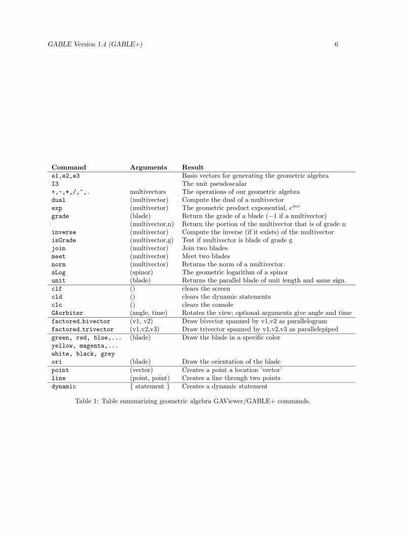
This section introduces the basics of the geometric algebra, and gives the GAViewer commandsfor performing the operations. Many of the objects have a graphical representation, and areautomatically displayed on the screen. Table 1 summarizes the GAViewer commands describedin this section and in the rest of this tutorial. We will introduce these routines gradually, as weneed them; the table is here just for reference. Some additional commands and details on someof the commands in this table can be found in the appendices. You can also get a summary ofcommands using ‘help()’ and ‘help(all)’.
GABLE Version 1.4 (GABLE+) 6
Command Arguments Resulte1,e2,e3 Basis vectors for generating the geometric algebraI3 The unit pseudoscalar+,-,*,/,^,. multivectors The operations of our geometric algebradual (multivector) Compute the dual of a multivectorexp (multivector) The geometric product exponential, emv
grade (blade) Return the grade of a blade (−1 if a multivector)(multivector,n) Return the portion of the multivector that is of grade n
inverse (multivector) Compute the inverse (if it exists) of the multivectorisGrade (multivector,g) Test if multivector is blade of grade gjoin (multivector) Join two bladesmeet (multivector) Meet two bladesnorm (multivector) Returns the norm of a multivector.sLog (spinor) The geometric logarithm of a spinorunit (blade) Returns the parallel blade of unit length and same sign.clf () clears the screencld () clears the dynamic statementsclc () clears the consoleGAorbiter (angle, time) Rotates the view; optional arguments give angle and timefactored bivector (v1, v2) Draw bivector spanned by v1,v2 as parallelogramfactored trivector (v1,v2,v3) Draw trivector spanned by v1,v2,v3 as parallelepipedgreen, red, blue,... (blade) Draw the blade in a specific coloryellow, magenta,...white, black, greyori (blade) Draw the orientation of the bladepoint (vector) Creates a point a location ’vector’line (point, point) Creates a line through two pointsdynamic { statement } Creates a dynamic statement
Table 1: Table summarizing geometric algebra GAViewer/GABLE+ commands.

GABLE Version 1.4 (GABLE+) 7
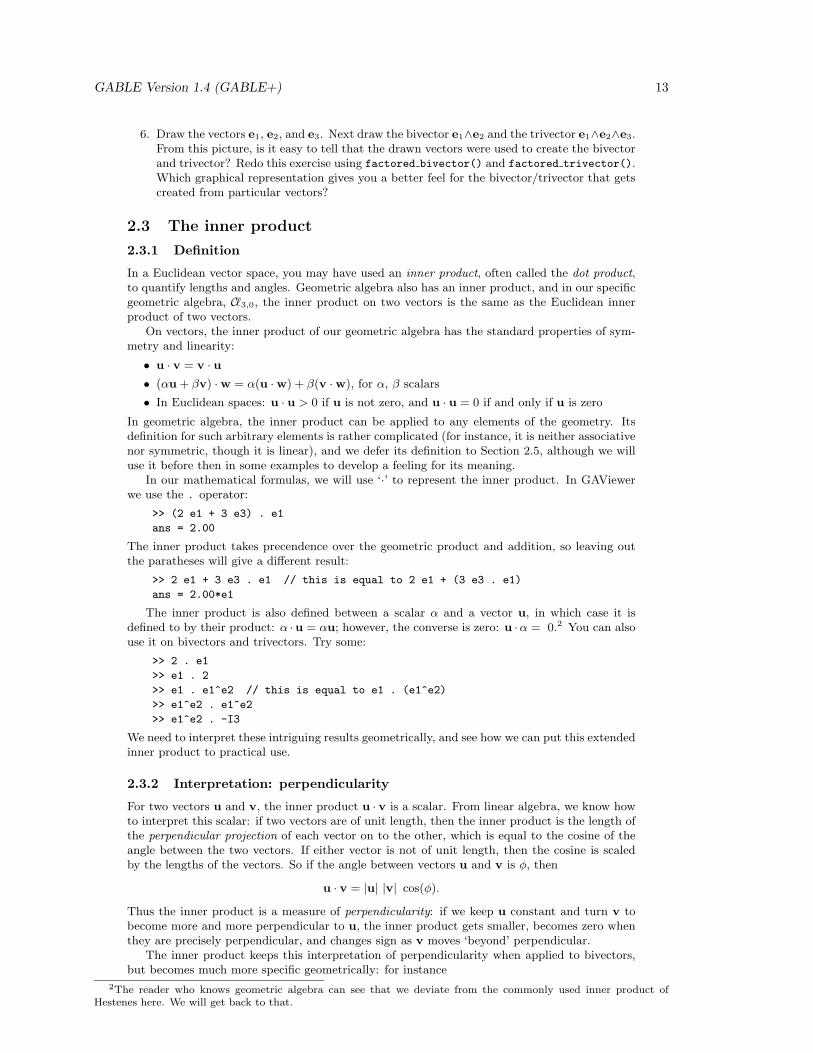
Figure 1: a = 3 e1 + 2 e3, b = e2,
2.1 Scalar product
The defining elements of geometric algebra are the vectors of a linear space of vectors overscalars. In our package, we use an orthonormal basis to represent this linear space, with vectorse1, e2, and e3, and we will always use integer or real numbers as our scalars.1 You can scaleand add these vectors in the usual manner. For example, to create the vector a = 3e1 + 2e2,you would type
>> a = 3 * e1 + 2 * e3
a = 3.00*e1 + 2.00*e3
or, since the ’space’ character is the geometric product in GAViewer:
>> a = 3 e1 + 2 e3
a = 3.00*e1 + 2.00*e3
The norm of a vector is its length (in the standard metric in Euclidean space):
>> // ... needs a
>> norm(a)
ans = 3.61
In GAViewer, when you assign a value to a variable in the global scope (i.e., on the console),the interpretation of that value gets drawn. There are three exceptions: when you terminatethe statement containing the assignment with a semicolon ’;’, when the value has no geometricinterpretation, or when GAViewer is unable to draw the interpretation (because we have notimplemented it yet, or due to roundoff errors).
For example, try the difference between
>> b = e2;
and
>> b = e2,
b = 1.00*e2
Your screen should now look something like Figure 1. Note that both vectors start at theorigin and have their arrow head at the end of the line segment away from the origin. If youwould like to understand the spatial relationship better, use the three mouse buttons to rotate/ translate your viewpoint, or type:
>> GAorbiter();
and the plot will turn 360 degrees over 10 seconds. You can get smaller rotations by giving itan argument; try GAorbiter(180);. If you give a second argument, you can change the timeover which it rotates; try GAorbiter(180,5);.
Scalars can not be drawn, but you can see their value on the console, in the object controlswindow on the right of GAViewer, and on the statusbar at the bottom GAViewer:
>> c = 2
>> select(c) // select() selects the current object
1Frames are a necessary crutch for input and output; but most of our computations will be independent of theframe of representation, in the sense that our equations and computations can be expressed in a coordinate-freemanner.

GABLE Version 1.4 (GABLE+) 8
2.2 The outer product
2.2.1 Definition
Geometric algebra has an outer product, often called a wedge product. The outer product hasthe properties of anti-symmetry, linearity and associativity. For vectors u, v, w we have:
• v ∧w = −w ∧ v, so that v ∧ v = 0
• u ∧ (v + w) = u ∧ v + u ∧w
• u ∧ (v ∧w) = (u ∧ v) ∧w
The outer product of a vector v with a scalar α, or of two scalars α and β, we define to be equalto the scalar product
α ∧ β = αβ and α ∧ v = αv,
and then use associativity to extend that to the evaluation of more involved terms.(The properties of the outer product of two vectors are similar to the properties of the cross
product for two vectors in 3D. Yet it results in a different geometrical object, as we will soonsee. We will discuss the correspondence between the two in Section 2.4.3).
2.2.2 Bivectors
In GAViewer, the circumflex symbol (ˆ) is used to take the outer product of objects. E.g., theouter product of e1 and e2 is formed by e1^e2. Here are some to try, and you may want toverify the results on paper using the definition:
>> 2^e2
>> e1^e2
>> e2^e1
>> e1 ^ (e1+e2)
>> (e1+e2) ^ (e1-e2)
The outcome of the wedge product of two vectors thus contains terms like α(e1 ∧ e2), etc.,which can not be simplified further to vectors or scalars. This outcome is therefore a new kindof object in our geometric algebra, called a bivector.
As you try more combinations, you find that any bivector can be expressed as a scalar-weighted linear combination of the standard bivectors e1 ∧ e2, e2 ∧ e3, e3 ∧ e1, formed by outerproduct between the vectors in the vector basis. This follows easily from the linearity and anti-symmetry properties in the definition of the outer product. These bivectors thus form a bivectorbasis (but as in the case of a basis for vectors, other bases may serve just as well). Algebraically,the set of bivectors in 3-dimensional space is therefore in itself a 3-dimensional linear space.
You can view a bivector as a directed area element, directed both in the sense of specifyinga plane and an orientation in that plane. In general, with φ denoting the angle from u to v andwith i the unit directed area of the (u,v)-plane, we can write:
u ∧ v = |u| |v| sin(φ)i.
You recognize that |u| |v| sin(φ) is the directed area spanned by u and v; and as u and v getmore parallel, this quantity becomes smaller. As you make the angle negative, the bivectorbecomes negative (in agreement with the anti-symmetry of the outer product since now u and vhave switched roles); this is what we mean by a directed area element. The i indicates the planein which this takes place; it is therefore a geometric ‘unit direction of dimension 2’ of what ismeasured.
Graphically we represent the bivector in GAViewer as a directed circle in the bivector plane.The area of the circle is the magnitude of the bivector. Arrows along a bivectors border canindicate the orientation, but in GAViewer you have to turn that on explicitly using the ori()
function.For example, let us draw some vectors, and then draw a bivector:
>> clf(); a = 2 e1 + e3, b = e2,
>> c = ori(e1^e2)
You should see in the graphics window something like Figure 2. Perform GAorbiter to appreciatethe spatial relationships better: note that the circle lies in the plane containing both e1 and e2.
The norm of a bivector is the absolute value of the area it represents:

GABLE Version 1.4 (GABLE+) 9
Figure 2: a = 2 e1 + e3, b = e2, c = e1^e2
>> norm((e1+e2)^e3)
ans =
1.4142
2.2.3 Trivectors
Taking the outer product of three vectors yields yet another object, which is naturally calleda trivector. It is a directed volume element. In 3-dimensional space, all such elements mustbe multiples of the unit directed volume element, which we denote by I3. (In other words,algebraically the trivectors of a 3-dimensional vector space form a 1-dimensional linear spacewith basis I3.) In an orthonormal basis e1, e2, e3 for our Euclidean 3-space, we equate it withthe volume spanned by the ‘right-handed’ frame: I3 ≡ e1 ∧ e2 ∧ e3. The unit directed volumeI3 is often called the (unit) pseudoscalar of 3-dimensional Euclidean space.
We have implemented I3 as I3. [[ but it gets cleared when they do clf(). ]] Verifythe outcome of the following expressions by hand, to get some dexterity in manipulations withthe wedge product on the basis of its definition:
>> e1^(e2^e3)
>> (e1^e2)^e3
>> e1^e2^e3
>> e3^e2^e1
>> e1^(e1+2*e2)^e3
>> e1^(e1+2*e2)^e1
>> norm(e1^e2^e3)
Notice that the trivector e3∧e2∧e1 equals −I3: these vectors in this order form a ‘left-handed’frame. The terms denoting ‘handedness’ are therefore not explicit conventions anymore, theyhave become part of the computational framework of geometric algebra as the signs of trivectors.The norm of a trivector is absolute value of the volume; if you need a signed scalar denoting thevolume of a trivector T, use T/I3.
Conceptually, a trivector represents an oriented volume. Graphically, we represent it by asphere, which we render transparently such that it won’t hide all objects inside it. The magnitudeof the trivector is represented by the volume of the sphere. To indicate the orientation (use theori() function again), we draw line segments emanating from the surface of the sphere; theorientation is indicated by whether these line segments go into or out of the sphere. Try
>> s1 = green(ori(I3))
>> s2 = red(ori(-0.5*I3))
2.2.4 Quadvectors?
If you try taking some outer products of four or more vectors, you will find that these areall zero. You may understand why this should be: since only three vectors in 3-space can beindependent, any fourth must be writable as a weighted sum of the other three; and then the

GABLE Version 1.4 (GABLE+) 10
anti-symmetry of the outer product kills any term in the expansion. For instance:
e1 ∧ e2 ∧ e3 ∧ (e1 + e2)
= e1 ∧ e2 ∧ e3 ∧ e1 + e1 ∧ e2 ∧ e3 ∧ e2
= (e1 ∧ e1) ∧ e2 ∧ e2 − e1 ∧ (e2 ∧ e2) ∧ e3 = 0.
So the highest order object that can exist in a 3-dimensional space is a trivector. But you canalso see that this is not a limitation of geometric algebra in general: if the space had moredimensions, the outer product would create the appropriate hyper-volumes.
If all we are interested in is planar geometry, then all vectors can be written as the linearcombination of two basis vectors, such as e1 and e2; in that case, the highest order object wouldbe a bivector. We would then call I2 ≡ e1 ∧ e2 a pseudoscalar of that 2-dimensional space. Inn-dimensional space, the pseudoscalar is the highest dimensional object in the space. It receivedthis rather strange name because it is ‘dual’ to a scalar, as we will see in Section 2.4.3.
2.2.5 0-vectors
In the same vein of the interpretation of k-vectors as geometrical k-dimensional subspaces basedin the origin, we can reinterpret the scalars geometrically. Since these are 0-vectors, they shouldrepresent a 0-dimensional subspace at the origin, i.e. geometrically, a scalar is a weightedpoint at the origin. This is a fully admissible geometric object, and therefore it should not besurprising that it is a member of the basis {1, e1, e2, e3, e1 ∧ e2, e2 ∧ e3, e3 ∧ e1, e1 ∧ e2 ∧ e3} ofthe geometric algebra of 3-dimensional space.
2.2.6 Use: parallelness and spanning subspaces
The outer product of two vectors u and v forms a bivector. When you keep u constant butmake v increasingly more parallel to it (by turning it in the (u,v)-plane), you find that thebivector remains in the same plane, but becomes smaller, for the area spanned by the vectorsdecreases. When the vectors are parallel, the bivector is zero; when they move beyond parallel(v turning to the ‘other side’ of u) the bivector reappears with opposite magnitude. Try this:
>> a = e1
>> b = e2
>> dynamic{c = ori(a ^ b),}
Drag the vectors a and b using the right mouse button, or assign them a different value on theconsole, like
>> a = e2 + 0.05 e1
The dynamic{} statement will be re-evaluated every time a, or b changes, adapting the bivectorc. The more parallel the vectors are, the smaller the bivector will be.
A bivector may thus be used as a measure of parallelness: in Euclidean space u ∧ v equalszero if and only if u and v are parallel, i.e., lie on the same 1-dimensional subspace. Note thatthis even holds for 1-dimensional space.
When you’re done with the example from above, use cld(); to remove the dynamic{}statement. Otherwise it will stick around and confuse you later on.
Similarly, a trivector is zero if and only if the three vectors that compose it lie in the sameplane (2-dimensional subspace). We then do not call them ‘parallel’; the customary expressionis ‘linearly dependent’, but the geometric intuition is the same. If the vectors are ‘almost’ in thesame plane, they span a ‘small’ trivector (relative to their norms times the unit pseudoscalar).
In fact, we can use a bivector B to represent a plane through the origin:
vector x in plane of B ⇐⇒ x ∧B = 0.
And this B even represents a directed plane, for we can say that a point y is at the ‘positiveside’ of the plane if y ∧B is a positive volume, i.e., a positive multiple of the unit pseudoscalarI3. We will come back to this powerful way of representing planes later (Section 3.7); but fornow you understand why we like to think of a bivector as a directed plane element.

GABLE Version 1.4 (GABLE+) 11
2.2.7 Blades and grades
We now have all the basic elements for our geometric algebra of 3-space: scalars, vectors,bivectors, and trivectors (pseudoscalars). We have constructed each of these from vectors andscalars using the outer product. There are some useful terms to describe this construction.
A blade is an object that can be written as the outer product of vectors. For instance, e1,or e1 ∧ (e1 + 2e2), or I3 ≡ e1 ∧ e2 ∧ e3.
The grade of a blade is the dimension of the subspace that the blade represents. So forinstance grade(e1 ∧ (e1 + e2 + e3)) = 2, and grade(I3) = 3. As you see, the outer product of aobject with a vector raises the grade of the object by one (or gives 0).
We can make general objects in our algebra by taking scalar-weighted sums of blades suchas 1 + e1 + e2 ∧ e3. Such objects are called multi-vectors. In this construction, a blade is calledan m-vector, with m the grade of the blade. In that sense, a scalar is a 0-vector. Often such amultivector is of mixed grade (do not worry about its geometrical interpretation yet).
In GAViewer, we have a routine grade that when given an object, returns the grade of thatobject. If the object is of mixed grade, grade returns -1. When invoked with a geometric objectand an integer, grade returns the portion of the geometric object of that grade. For example,
>> grade(e1+I3,1)
ans = 1.00*e1
>> grade(e1+I3,3)
ans = 1.00*e1^e2^e3
To test if an object is of a particular grade, use the isGrade command:
>> isGrade(e1^e2,1)
ans = 0
>> isGrade(e1^e2,2)
ans = 1.0
In this context of blades and grades, there is a peculiarity of 3-dimensional space that doesnot carry over to higher dimensions: in 3-space (or 2-space, or 1-space), any multivector that isnot of mixed grade can be factored into a blade. For example, we can rewrite e1 ∧ e2 + e2 ∧ e3
as (e1−e3)∧e2. The former is the sum of two bivectors (and thus not in blade form), while thelatter is the outer product of two vectors (and is therefore obviously a blade). In 4-dimensionalspace, this fails: e1 ∧ e2 + e3 ∧ e4 cannot be rewritten as the outer product of two vectors.
2.2.8 Other ways of visualizing the outer product
The interpretation of the bivector as a directed circle, which we have used so far, is not whateveryone uses to visualize them. The standard interpretation works directly with the outerproduct. If you have e1 ∧ (e1 + e2), then for the standard interpretation, we construct theparallelogram having e1 and e1 + e2 as two of its sides. Graphically, we would draw the vector(e1 +e2) starting from the head of e1. The area of this parallelogram is the area of the bivector,and the two vectors give the orientation.
You can see this interpretation of the bivector in GABLE+ using by typing
>> a = factored_bivector(e1, e1 + e2)
Note, however, that the particular vectors used to construct the bivector are not unique. Anytwo vectors in this plane that form a parallelogram of the same directed area give the samebivector. For example,
>> //...
>> b = red(factored_bivector(e1, e2))
will draw a second red parallelogram (a square) that overlaps the first parallelogram. Althoughthese are two different parallelograms, they are coplanar and have the same directed area,therefore they represent the same bivector. (If you are having trouble seeing any of the twobivectors, slide down the alpha value (in the object controls window) for both of them.)
Using GAViewer, you can test that these represent the same bivector by using the equalityoperator:
>> e1^(e1+e2) == e1^e2
ans = 1.00

GABLE Version 1.4 (GABLE+) 12
In GAViewer, a result of ‘1’ for a Boolean test means “true” and a result of ‘0’ means “false.”In our example, this means the geometric objects are the same, which we can also prove alge-braically:
e1 ∧ (e1 + e2) = e1 ∧ e1 + e1 ∧ e2 = e1 ∧ e2
Note that the area is oriented. In particular, if we reverse the order of the vectors in theouter product, we get a different result:
>> e1^e2 == e2^e1
ans = 0
However, they only differ by a sign:
>> e1^e2 == -e2^e1
ans = 1.00
This is a result of the bivector representing a directed area: if we reverse the order of thearguments, then we get the opposite direction.
More generally, we can think of the bivector as representing any directed area within somesimple, closed, directed curve. (To prove this we would need to develop a calculus; we willnot do so in this introduction, so please just accept this statement.) We used a circle for ourrepresentation since we often will not have the creating vectors for a bivector. Indeed, dependingon how we constructed the bivector such vectors may not exist, for example when we take thedual (Section 2.4.3) of a vector. While we may use any closed curve of the appropriate area,the circle is the closed curve with perfect symmetry. In our rendering of the bivector, the areaof the circle indicates the area of the bivector; to indicate the orientation of the area, we drawarrows along its rim.
In a similar manner, we can view a trivector as a parallelepiped. Clear the screen, then run
>> t = factored_trivector(e1,e1+e2,e3)
>> GAorbiter();
to see the parallelepiped constructed for a trivector.
2.2.9 Summary
In this section we have seen the outer product, which combines elements of geometric algebra toform higher dimensional elements. In particular, the outer product of two vectors is a directedarea element that spans the space containing those two vectors. When applied to other bladesof our space, we get higher dimensional directed volume elements.
If the vectors we combine with the outer product are linearly dependent, then the result ofthe outer product will be zero; if they are ‘almost linearly dependent’ in the sense of almostaligned, the outer product will be small. Therefore the outer product provides a quantitativeand computational way to treat linear dependence.
Exercises
1. Draw the following bivectors e1 ∧ e2, e2 ∧ e3, and e3 ∧ e1, each in a different color. Usefunction like red(), white() and blue() to set the color.
2. Redraw the bivectors of the previous exercise using factored bivector(). Based on thisand the previous exercise, do you have a feeling that these bivectors are orthogonal?
3. Draw using factored bivector() the bivectors e1 ∧ e2 and e1 ∧ (e2 + 3e1). From thispicture, do you get a feeling whether or not these two bivectors are equal? Test theirequality by comparing them with the == operator.
4. Draw the bivectors e1 ∧ e2 and e2 ∧ e1. Use the ori() function to draw the orientationof the bivectors. Are these two bivectors the same? Hint: Notice how the arrows pointin opposite directions. Repeat this exercise using factored bivector() and comment onthe results.
5. Draw the trivector e1 ∧ e2 ∧ e3 the ordinary way (use the ori() function to draw the ori-entation), and using factored trivector(). Now clear the screen and draw the trivectore1∧e3∧e2 with both drawing routines. Which graphical representation gives you a betterfeel for orientation?
GABLE Version 1.4 (GABLE+) 13
6. Draw the vectors e1, e2, and e3. Next draw the bivector e1∧e2 and the trivector e1∧e2∧e3.From this picture, is it easy to tell that the drawn vectors were used to create the bivectorand trivector? Redo this exercise using factored bivector() and factored trivector().Which graphical representation gives you a better feel for the bivector/trivector that getscreated from particular vectors?
2.3 The inner product
2.3.1 Definition
In a Euclidean vector space, you may have used an inner product, often called the dot product,to quantify lengths and angles. Geometric algebra also has an inner product, and in our specificgeometric algebra, C 3,0, the inner product on two vectors is the same as the Euclidean innerproduct of two vectors.
On vectors, the inner product of our geometric algebra has the standard properties of sym-metry and linearity:
• u · v = v · u• (αu + βv) ·w = α(u ·w) + β(v ·w), for α, β scalars
• In Euclidean spaces: u · u > 0 if u is not zero, and u · u = 0 if and only if u is zero
In geometric algebra, the inner product can be applied to any elements of the geometry. Itsdefinition for such arbitrary elements is rather complicated (for instance, it is neither associativenor symmetric, though it is linear), and we defer its definition to Section 2.5, although we willuse it before then in some examples to develop a feeling for its meaning.
In our mathematical formulas, we will use ‘·’ to represent the inner product. In GAViewerwe use the . operator:
>> (2 e1 + 3 e3) . e1
ans = 2.00
The inner product takes precendence over the geometric product and addition, so leaving outthe paratheses will give a different result:
>> 2 e1 + 3 e3 . e1 // this is equal to 2 e1 + (3 e3 . e1)
ans = 2.00*e1
The inner product is also defined between a scalar α and a vector u, in which case it isdefined to by their product: α ·u = αu; however, the converse is zero: u ·α = 0.2 You can alsouse it on bivectors and trivectors. Try some:
>> 2 . e1
>> e1 . 2
>> e1 . e1^e2 // this is equal to e1 . (e1^e2)
>> e1^e2 . e1^e2
>> e1^e2 . -I3
We need to interpret these intriguing results geometrically, and see how we can put this extendedinner product to practical use.
2.3.2 Interpretation: perpendicularity
For two vectors u and v, the inner product u · v is a scalar. From linear algebra, we know howto interpret this scalar: if two vectors are of unit length, then the inner product is the length ofthe perpendicular projection of each vector on to the other, which is equal to the cosine of theangle between the two vectors. If either vector is not of unit length, then the cosine is scaledby the lengths of the vectors. So if the angle between vectors u and v is φ, then
u · v = |u| |v| cos(φ).
Thus the inner product is a measure of perpendicularity: if we keep u constant and turn v tobecome more and more perpendicular to u, the inner product gets smaller, becomes zero whenthey are precisely perpendicular, and changes sign as v moves ‘beyond’ perpendicular.
The inner product keeps this interpretation of perpendicularity when applied to bivectors,but becomes much more specific geometrically: for instance
2The reader who knows geometric algebra can see that we deviate from the commonly used inner product ofHestenes here. We will get back to that.

GABLE Version 1.4 (GABLE+) 14
x ·B is a vector in the B-plane perpendicular to x.
Let us visualize this:
>> clf();
>> B = e1^e2
>> x = yellow(e1+e3) // draw x in yellow
>> dynamic{ xiB = x . B, }
Because we have made xiB¯
dynamic, it will be recomputed when you can modify B or x. Forinstance, use ctrl-right mouse button-drag to move the yellow vector x and see what happens.
When you’re done with this example, use cld(); to remove the dynamic{} statement.Note that the result is also perpendicular to x and in the B-plane if the vector x was in the
B-plane to begin with.
>> clf();
>> B = e1^e2
>> b = yellow(e1)
>> biB = b . B
So in a sense, the operation ‘·B’, applied to a vector b in the B-plane (so that b ∧ B = 0),produces the perpendicular to b in that plane, the complement to b in the B-plane. Thisgeneralizes, as we will see later (Section 4.2).
Even with a trivector, the interpretation of the inner product as producing a perpendicularresult remains:
>> clf();
>> x = e1+e3
>> xiI3 = x . I3
>> GAorbiter();
The inner product x · I3 is now the bivector representing the plane perpendicular to x. Con-versely, the inner product of a bivector with a trivector produces a vector perpendicular to theplane of the bivector:
>> clf();
>> B = (e1 + e2) ^ e3
>> BiI3 = B . I3
>> GAorbiter();
You begin to see how conveniently the inner and outer product work together to produce simpleexpressions for such constructions.
In general, for blades of different grades, if the grade of the first argument is less than thegrade of the second argument, then their inner product is a blade whose grade is the difference ingrades of the two objects, lies in the subspace of the object of higher grade, and is perpendicularto the object of lower grade. The inner product is thus grade decreasing. However, if the firstargument has a larger grade than the second, our inner product is zero (because of this grade-reducing property it is also known as a contraction, and you cannot contract something biggeronto something smaller).3
But what happens if we take the inner product of two blades of the same grade? We alreadyknow that the inner product of two vectors yields a scalar. Try taking the inner product of twobivectors:
>> e1^e2 . e2^e3
>> e1^e2 . e1^e2
In both cases, the result is a scalar; in the first example, the result is 0, while in the secondexample, it is −1. Likewise, if we take the inner product of the pseudoscalar with itself theresult is a scalar. In general, the inner product of two blades of the same grade results in ascalar.
2.3.3 Summary
The inner product is a generalization of the dot product, and may be applied to any two elementsof our space. When applied to vectors, it is the familiar dot product. More generally, the innerproduct is associated with perpendicularity.
3You should be aware that the more commonly used ‘Hestenes inner product’ is not a contraction. More aboutthis later.

GABLE Version 1.4 (GABLE+) 15
2.4 The geometric product
2.4.1 Definition
We have seen how the inner and outer product of two vectors specify aspects of their perpen-dicularity and parallelness, but neither gives the complete relationship between the two vectors.So it makes sense to combine the two products in a new product. This is the geometric product,and it is amazingly powerful.
We denote the geometric product of objects by writing them next to each other leaving themultiplication symbol understood. For vectors u and v, we define:
u v = u ∧ v + u · v. (1)
This is therefore an object of mixed grade: it has a scalar part u · v and a bivector part u ∧ v.This mixed grade is not a problem, as geometric algebra spans a linear space in which suchscalar-weighted combinations of blades are perfectly permissible.
Changing the order of u and v gives:
v u = v ∧ u + u · v = −u ∧ v + u · v,
so the geometric product is neither fully symmetric, nor fully anti-symmetric.With the geometric product defined, we can use it as the basis of geometric algebra, and
view the inner and outer products as secondary, derived constructions. For instance, for vectorswe we can retrieve the inner and outer products as its symmetric and anti-symmetric parts,respectively:
u · v = 12(uv + vu) (2)
u ∧ v = 12(uv − vu) (3)
and these formulas can be extended to arbitrary multivectors (see Section 2.5). Although theproducts algebraically have this relationship to each other (with the geometric product beingthe more fundamental one), yet we will show that geometrically it is convenient to think of themas three basic products, each with their own geometric annotations and usage. Inner productand outer product are indeed highly meaningful ‘macros’ for geometric algebra.
In GAViewer, you can use the * operator for the geometric product, but you can also omitit and simply use a space ’ ’ for the geometric product. In this text we will omit the *. Usethe following examples to play around with geometric product a bit– but check the outcomesby hand to familiarize yourself with the computations.
>> e1 (e1 + e2) // this is equal to e1 * (e1 + e2)
>> (e1 + e2)(e1 + e3)
>> (e1 + e2)(e1 + e2)
>> e1 e2
>> e1 e1
The geometric product is extended by linearity and associativity to general multivectors (Sec-tion 2.5), which is how we have implemented it. A geometric product of general multivectorsmay produce multivector with many different grades:
>> (1 + e1)(e1 e2 + e1^e2^e3 + e1.e2^e3)
ans = 1.00*e2 + 1.00*e2^e3 + 1.00*e1^e2 + 1.00*e1^e2^e3
Here GAViewer may complain that the multivector has no interpretation. You can still use itin computation, but GAViewer can not draw it.
The geometric interpretation of the geometric product is more difficult than the geometricinterpretations of vectors, bivectors, and trivectors. By Equation 1,
>> e1 (e1 + 2 e2)
results in the scalar e1 · (e1 + 2e2) = e1 · e1 = 1 and a bivector e1 ∧ (e1 + 2e2) = 2e1 ∧ e2 andit is hard to understand what that means. We will soon recognize that the geometric productproduces a geometric operator rather than a geometric object, and that therefore we had bettervisualize it through its effect on objects, rather than by itself. GAViewer draws the multivectorkind of like a bivector with a arrow in it, which suggests that it has something to do withrotation.

GABLE Version 1.4 (GABLE+) 16
2.4.2 Invertibility of the geometric product
The inner product and outer product each specify the relationships between vectors incompletely,so they can not be inverted (e.g., knowing the value of the inner product of an unknown vector xwith a known vector u does not tell you what x is). However, the geometric product is invertible.This is extremely powerful in computations.
Still, not all multivectors have inverses in general geometric algebras. Fortunately, in thegeometric algebra of Euclidean space, subspaces (represented as blades, i.e., multivectors of asingle grade) do. Thus, for each blade A 6= 0 in Euclidean space, we can find A−1 such thatAA−1 = 1.
Let us first take a linear subspace, characterized by a vector v. (Why does a vector charac-terize a linear subspace? Because x ∧ v = 0 characterizes all vectors x in this subspace.) Whatis its inverse? Think about this, then ask GAViewer:
>> v = 2 e1
>> iv = inverse(v)
>> v iv
>> iv v
So, as you thought, the inverse of a vector is parallel to the vector, but differs by a scalar factor:
v−1 =v
v · v .
This is easily verified:
v(v/(v · v)) = (vv)/(v · v) = (v · v + v ∧ v)/(v · v) = (v · v + 0)/(v · v) = 1.
Now consider a two-dimensional subspace, characterized by a bivector B. For instance, whatis the inverse of 2e1 ∧ e2, where the basis {e1, e2, e3} is orthonormal? In such a basis we have:
e1 e1 = e1 · e1 = 1, etc. and e1 e2 = e1 ∧ e2, etc. (4)
With this, we observe that
(e1 ∧ e2) (e1 ∧ e2) = (e1e2)(e1e2) = e1(e2e1)e2 = −(e1e1)(e2e2) = −1, (5)
so, in the sense of the geometric product: the square of a bivector is negative. Then the inverseis simple to determine: (2e1 ∧ e2)−1 = − 1
2(e1 ∧ e2) = 1
2e2 ∧ e1. In general, in C 3,0
B−1 =B
B ·B .
The inverse of a pseudoscalar αI3 is also easy. Observe that
I3I3 = (e1 ∧ e2 ∧ e3)(e1 ∧ e2 ∧ e3)
= e1e2e3e1e2e3 = −e2e1e3e1e2e3
= e2e3e1e1e2e3 = e2e3e2e3
= −e3e2e2e3 = −e3e3 = −1
Thus, in our algebra the inverse of αI3 is:
(αI3)−1 = −I3/α.
In GAViewer, use inverse() to compute the inverse of a geometric object. As a short-hand for B*inverse(A), you may write B/A. Note that the geometric product is not in generalcommutative, so we would write inverse(A)*B as (1/A)*B, which is rarely equal to B/A.
2.4.3 Duality
The dual of an element A of our geometric algebra is defined to be
dualA ≡ A/I3 = −AI3, (6)
and in GAViewer the function dual() returns the dual of an object. The dual of a bladerepresenting a subspace is a blade representing the orthogonal complement of that subspace,i.e., the space of all vectors perpendicular to it. This is a common construction, and it is greatto have it in such a simple form: just divide by I3.
For example, type the following:

GABLE Version 1.4 (GABLE+) 17
>> clf();
>> a = e1
>> b = dual(e1)
The red vector represents e1; the blue circle represents the dual of e1, which is -e2^e3 as shownby the following derivation:
dual(e1) = e1I−13 = e1(e1 ∧ e2 ∧ e3)−1
= e1(e1e2e3)−1 = −e1e1e2e3
= −e2e3 = −e2 ∧ e3
The construction is more striking for more arbitrary vectors, of course (see exercises).Note that for a blade U we have grade (dual(U)) = 3 − grade (U), so that the dual of a
scalar is a pseudoscalar and vice versa: dual(1) = −I3 and dual(I3) = 1 (this is true in anyspace and partly explains the name ‘pseudoscalar’ for the n-dimensional volume element).
As a consequence of this rule on grades, the dual relationship between vectors and bivectorsis only valid in 3-dimensional space. In 3-space, we may characterize a plane (which is reallya bivector) dually by a vector; that vector is commonly called the normal vector of the plane.We now see that it is the dual of the bivector. Indeed, both of the following two equationscharacterize the same plane B:
x ∧B = 0 and x · dual(B) = 0.
We recognize the latter as the ‘normal equation’ of the plane B, the inner product of a vectorx with the normal vector n ≡ dual(B) = B/I3.
This is an example of a duality relationship between the outer product and inner product.Since the outer product produces an element of geometric algebra, we can take its dual. Onecan then prove (nice exercise, try it for vectors)
dual(u ∧ v) = u · dual(v) and dual(u · v) = u ∧ dual(v) (7)
for any multivectors u and v from the geometric algebra of the space with the pseudoscalar I3
used to define the dual.This is a good moment to explain how the 3-dimensional cross product of vectors fits into
geometric algebra. The cross product obeys
u× v = dual(u ∧ v).
You can see this with the following GABLE+ commands:
>> clf();
>> a = e1 + 0.5 e2
>> b = e1 + e2 + e3
>> B = a ^ b
>> d = green(dual(B))
>> GAorbiter();
Here we see that the red vector is perpendicular to both of the blue vectors. To check that thedual matches the cross-product, print the dual of B compare it with you own computation ofthe cross product.
So we could define the cross product using the above equation. However, we will not do so,for two reasons. Firstly, the cross product is too particular for 3-dimensional space; in no otherspace is the dual of a ‘span of vectors’ a vector of that space. And secondly, its only use isto characterize planes and rotations. Geometric algebra offers a much more convenient way tocharacterize those, directly through bivectors. We have seen this for planes and we will see itfor rotations soon. Since these bivector characterizations are valid in arbitrary dimensions, weprefer them to any specific, 3D-only construction. So: we will not need the cross product.
Exercises
1. Determine the subspace perpendicular to the vector e1 + 0.2 e3.
2. Determine the subspace perpendicular to the plane spanned by the vectors e1 + 0.3 e3 ande2 + 0.5 e3, in one line of GAViewer.

GABLE Version 1.4 (GABLE+) 18
3. Prove Equation 7.
4. We used the geometric product to define the dual. We can also make the dual using the in-ner product (thus directly conveying the intuition of ‘orthogonal complement’). Give sucha formulation of the dual in a way that is equivalent to the geometric product formulationof the dual and show this equivalence.
2.4.4 Summary
The geometric product is a third product of our geometric algebra. Unlike the inner and outerproducts, the geometric product is invertible, which is useful when doing algebraic manipula-tions. In Section 3, we will see geometric interpretations of the geometric product.
2.5 Extension of the products to general multivectors
We have stated that the inner, outer, and geometric products can be generalized to arbitrarymultivectors. In this section, we will first show how to extend the definition of the geometricproduct to general multivectors. Once we have that, it is easy to extend the inner and outerproducts.
For general objects of geometric algebra, the geometric product can be defined as follows(this is not the only way, but it is the most easy to understand). In the n-dimensional vectorspace considered, introduce an orthogonal basis {e1, e2, · · · , en}. Use the outer product toextend this to a basis for the whole geometric algebra (the one containing e1 ∧ e2, etcetera).Any multivector can be written as a weighted sum of basis elements on this extended basis.The geometric product is defined to be linear and associative in its arguments, and distributiveover +, so it is sufficient to defined what the result is of combining two arbitrary elements ofthe extended basis. We first observe that the desired compatibility with Equation 1 combinedwith the orthogonality of the basis vectors leads to
eiej = −ejei if i 6= j (8)
because on the orthogonal basis, effectively eiej equals ei ∧ ej if i 6= j. If i = j, Equation 1gives the scalar result ei · ei, which in our Euclidean space equals 1.4 So we have
eiei = 1. (9)
This is now enough to define the geometric product of any elements in the geometric algebra.For instance (2+e1∧e2)(e1 +e2∧e3) is expanded by distributivity over + to 2e1 +(e1∧e2)e1 +2(e2∧e3)+(e1∧e2)(e2∧e3). The term (e1∧e2)e1 in this equals (e1e2)e1, and by associativitythis equals e1e2e1. We apply Equation 8 to get −e1e1e2, and then Equation 9 to get −e2.The other terms are computed in a similar way. Note that this definition is heavily based onthe introduction of an orthogonal basis (which is somewhat inelegant); other definitions manageto avoid that. You may also think that all these expansions make the geometric product anexpensive operation. But the above was just to show how those minimal definitions actuallydefine the outcome mathematically; a more practical computation scheme using matrices onthe extended basis is what we used to make the orginal GABLE (such details may be found in[15, 16]).
Now that we have defined the general geometric product, it is easy to generalize both theinner and outer products. Both products are linear in their arguments, and so are sufficientlyspecified when we say what they do on blades. For instance, if we would want to know theoutcome of (A1 + A2) · (B1 + B2) (where the index denotes the grade of the blades involved),then this can be written out as A1 ·B1 + A1 ·B2 + A2 ·B1 + A2 ·B2.
For a blade U of grade r, and a blade V of grade s, the definitions for inner and outerproducts are:
U ·V = grade(UV, s− r)U ∧V = grade(UV, s+ r).
4 To get a general geometric algebra, of a space with a quadratic form (‘metric’) Q, this is set to some specifiedscalar Q(ei), usually taken to be +1 or −1. The sign of Q(ei) is called the signature of ei.
GABLE Version 1.4 (GABLE+) 19
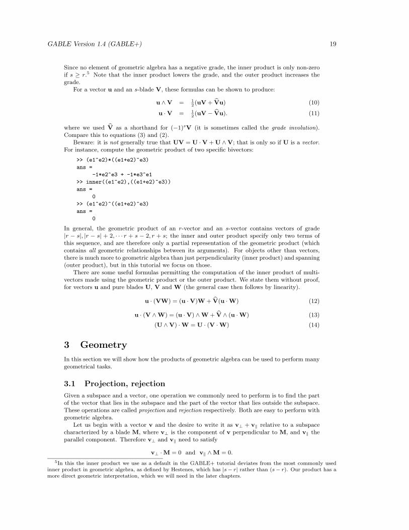
Since no element of geometric algebra has a negative grade, the inner product is only non-zeroif s ≥ r.5 Note that the inner product lowers the grade, and the outer product increases thegrade.
For a vector u and an s-blade V, these formulas can be shown to produce:
u ∧V = 12(uV + Vu) (10)
u ·V = 12(uV − Vu). (11)
where we used V as a shorthand for (−1)sV (it is sometimes called the grade involution).Compare this to equations (3) and (2).
Beware: it is not generally true that UV = U ·V + U ∧V; that is only so if U is a vector.For instance, compute the geometric product of two specific bivectors:
>> (e1^e2)*((e1+e2)^e3)
ans =
-1*e2^e3 + -1*e3^e1
>> inner((e1^e2),((e1+e2)^e3))
ans =
0
>> (e1^e2)^((e1+e2)^e3)
ans =
0
In general, the geometric product of an r-vector and an s-vector contains vectors of grade|r − s|, |r − s| + 2, · · · r + s − 2, r + s; the inner and outer product specify only two terms ofthis sequence, and are therefore only a partial representation of the geometric product (whichcontains all geometric relationships between its arguments). For objects other than vectors,there is much more to geometric algebra than just perpendicularity (inner product) and spanning(outer product), but in this tutorial we focus on those.
There are some useful formulas permitting the computation of the inner product of multi-vectors made using the geometric product or the outer product. We state them without proof,for vectors u and pure blades U, V and W (the general case then follows by linearity).
u · (VW) = (u ·V)W + V(u ·W) (12)
u · (V ∧W) = (u ·V) ∧W + V ∧ (u ·W) (13)
(U ∧V) ·W = U · (V ·W) (14)
3 Geometry
In this section we will show how the products of geometric algebra can be used to perform manygeometrical tasks.
3.1 Projection, rejection
Given a subspace and a vector, one operation we commonly need to perform is to find the partof the vector that lies in the subspace and the part of the vector that lies outside the subspace.These operations are called projection and rejection respectively. Both are easy to perform withgeometric algebra.
Let us begin with a vector v and the desire to write it as v⊥ + v‖ relative to a subspacecharacterized by a blade M, where v⊥ is the component of v perpendicular to M, and v‖ theparallel component. Therefore v⊥ and v‖ need to satisfy
v⊥ ·M = 0 and v‖ ∧M = 0.
5In this the inner product we use as a default in the GABLE+ tutorial deviates from the most commonly usedinner product in geometric algebra, as defined by Hestenes, which has |s− r| rather than (s− r). Our product has amore direct geometric interpretation, which we will need in the later chapters.

GABLE Version 1.4 (GABLE+) 20
Thus
v⊥M = v⊥ ·M + v⊥ ∧M
= v⊥ ∧M
= v⊥ ∧M + v‖ ∧M
= v ∧M.
But we can divide by the blade M, on both sides, so we obtain:
v⊥ = (v ∧M)/M (15)
A similar derivation shows thatv‖ = (v ·M)/M. (16)
These are the general projection and rejection formulas for a vector v relative to any subspacewith invertible blade M, in any number of dimensions. Powerful stuff!
It is important to visualize what is going on. Take M to be a 2-blade, determining a plane.Then v∧M is a volume spanned by v with that plane. It is a ‘reshapable’ volume: any vector vthat has its endpoint on the plane parallel to M, through v’s endpoint, spans the same trivector.The division by M in the formula for the projection demands the factoring of this volume intoa component M, and therefore returns what is left: the unique vector perpendicular to M thatspans the volume. This is a general property:
Dividing a space B by a subspace A produces the orthogonal complement to A in B.
If A is not a proper subspace, other things happen that we’ll cover later.These relationships can be seen in GAViewer. To begin, clear the graphics screen (clf())
and draw a bivector. For this demonstration, we will use factored bivector() to draw thegraphical representation of a bivector. Next, draw a vector that lies outside the plane of thisbivector:
>> clf();
>> B = factored_bivector(e1,e1+e2)
>> v = 1.5 e1 + e2 / 3 + e3
To get a better feel for the 3D relationships, use the mouse or GAorbiter() to rotate aroundthe scene a bit.
We can now type our formulas for the perpendicular and parallel parts of v directly intoGAViewer and draw the resulting perpendicular and parallel components of v relative to B:
>> //... needs v,B
>> vpar = green(v.B / B)
>> vperp = magenta(v^B / B)
We stated that this computation works for any subspace B. In particular, we can set B to be avector, and the same computations for vpar and vperp work. Try this!
As we will see later (but you could try it now), you may project a bivector A onto a bivectorB using the ‘same’ formula: A‖ = (A ·B)/B. However, the rejection of the bivector is now notobtained by A⊥ = (A∧B)/B, (which is zero since quadvectors do not exist in 3D), but simplyby A⊥ = A −A‖ (a formula that also works in the previous case where A is a vector). Moreabout the relationships of subspaces in Section 4.
Exercises
1. Redo the example of projection and rejection using the same v as above, but with B=e1+e2.
2. Let v = −3e1 − 2e2 and let B = 2e2 ∧ (e3 + 3e1). Compute the projection and rejectionof v by B. Draw v, B, and this projection and rejection. Try this exercise once usingfactored bivector() to draw B and a second time using draw to draw B.
3. With the same v and B as the previous exercise, study how the rejection formula works:first draw v ∧ B using factored trivector(); as decomposition use v, v · B and theprojection P((v),B). Then draw that trivector again in a decomposition that uses therejection.
4. Prove the formula for projection: v‖ = (v ·M)/M.

GABLE Version 1.4 (GABLE+) 21
5. (Not easy!) Using Equations 12, 13 and 14, show that
((a ∧ b) ·M)/M = a‖ ∧ b‖
(still a useful exercise!). This gives two ways to compute the projection of a bivector a∧brelative to a blade M. Which do you prefer and why?
3.2 Orthogonalization
Geometric algebra does not require the representation of its elements in terms of a particularbasis of vectors. Therefore the specific treatment of issues like orthogonalization are much lessnecessary. Yet it is sometimes convenient to have an orthogonal basis, and they are simple toconstruct using our products.
Suppose we have a set of three vectors u, v, w, and would like to form them into anorthogonal basis. We arbitrarily keep u as one of the vectors of the perpendicularized frame,which will have vectors denoted by primes:
u′ ≡ u.
Then we form the rejection of v by u′, which is perpendicular to u′:
v′ ≡ (v ∧ u′)/u′
Now we take the rejection of w by u′ ∧ v′, which is perpendicular to both u′ and v′:
w′ ≡ (w ∧ u′ ∧ v′)/(u′ ∧ v′)
and we are done. (This is the Gram-Schmidt orthogonalization procedure, rewritten in geometricalgebra.) Here’s an example (no need to type it, use GAblock(1);, see section 1.2!):
>> // GAblock(1)
>> // ORTHOGONALIZATION
>> clf();
>> // the original vectors
>> u = green( e1+e2 ),
>> v = green( 0.3*e1 + 0.6*e2 - 0.8*e3 ),
>> w = green( e1 -0.2*e2 + 0.5*e3 ),
>> // and orthognalized:
>> u_p = red( u ),
>> v_p = red( (v^u_p)/u_p ),
>> w_p = red( (w^u_p^v_p)/(u_p^v_p) ),
>> GAorbiter();
You might want to draw the duals to show the perpendicularity of the resulting basis moreclearly (see Exercise 1).
Note that in this construction, v′∧u′ = v′u′ = v∧u, and w′∧v′∧u′ = w′(v′u′) = w∧v∧u,so that it preserves the trivector spanned by the basis, in magnitude and orientation. Checkthis in GAViewer:
>> (u ^ v ^ w) == (u_p ^ v_p ^ w_p)
ans = 1.00
As an exercise, you might want to give the algorithm for n-dimensional orthogonalization.
Exercises
1. Convince yourself that up, vp and wp are orthogonal, using graphics routines to exploretheir construction. You might for instance draw dual(up), and in that plane study vp andwp.

GABLE Version 1.4 (GABLE+) 22
mr v
v
v
Figure 3: Reflecting v through m.
3.3 Reflection
Suppose we wish to reflect a vector v through some subspace (a vector, a plane, whatever). Ina geometric algebra, this subspace is naturally described by a blade, so we will look at reflectingv through a unit blade M. If we write v as
v = v⊥ + v‖,
where v⊥ is the part of v perpendicular to M and v‖ is the part parallel to M (we derivedformulas for both in the Section 3.1), then r, the reflection of v through M, is given by
r = v‖ − v⊥.
Using our formulas for the parallel and perpendicular parts of v relative to M, we see that
r = v‖ − v⊥
= (v ·M)M−1 − (v ∧M)M−1
= 12(vM− Mv)M−1 − 1
2(vM + Mv)M−1
= −MvM−1.
This is an interestingly simple expression for such arbitrary reflections.Let us see what the formula yields for specific choices of the blade we reflect in. In 3D, there
are four possibilities for the blades.
• scalar: M = 1The scalar, viewed as a subspace, is a point at the origin (see Section 2.2.5). And indeed,our reflection formula yields v → − v, which is clearly a point reflection in the origin.
• vector: M = uLet the blade M characterize the reflecting subspace be a unit vector u; then the reflectionis relative to a line in direction u. This gives
r = uvu.
An attractive formula for a basic process!
• bivector M = BFor a plane in 3D characterized by a unit bivector B (so that B2 = −1, and thereforeB−1 = −B), we obtain
r = BvB.
We could also write this in terms of the dual to the plane, i.e., the normal vector n definedas n = BI−1
3 :r = BvB = nI3vnI3 = nI2
3vn = −nvn.
(It is a good exercise to prove r = −nvn for reflection in a hyperplane dual to n inarbitrary-dimensional space.)
You can see this in GAViewer with the following sequence of commands:
>> clf();
>> v = yellow(e1 + 2 e3)
>> M = e1 ^ e2
>> v_r = M v M

GABLE Version 1.4 (GABLE+) 23
• volume M = I3
Since I3 = −I3 and I3 commutes with v, this gives v → v. Reflection in the containingspace is the identity, since v⊥ = 0.
To develop the formula for the reflection of an arbitrary blade of grade k in the blade M ofgrade m, first see what happens for the geometric product of the reflection of k vectors:
(−Mu1M−1)(−Mu2M
−1) · · · (−MukM−1) =
= (−1)kMu1M−1Mu2M
−1 · · · MumM−1
= (−1)k+kmMu1M−1Mu2M
−1 · · ·MukM−1
= (−1)k(m+1)Mu1u2 · · ·ukM−1.
Therefore:
X even grade : X→MXM−1
X odd grade : X→ −MXM−1
A bit complicated; but that is how reflections are for such subspaces.By the way, you see from this what happens if you reflect a plane characterized by a bivec-
tor B, relative to the origin: it is preserved. However, its normal would reflect, and that isundesirable. In the past, when people could only characterize planes by normal vectors, theytherefore had to make two kinds of vectors: position vectors which do reflect in the origin, and‘axial’ vectors which don’t, and realize that a normal vector is an axial vector. Using bivectorsdirectly to characterize planes, we have no need of such a strange distinction: the algebra andits semantics simplifies by admitting objects of higher grade!
Exercises
1. Reflect the bivector B = (e1^e2 + 2/3 e2^e3 + e3^e1/3) through the plane spanned bythe bivector M = e1^e2. Note carefully what happens to the orientation of the bivector.Is that what you expected?
2. Reflect the pseudoscalar I3 through a bivector. Note the orientation.
3. Do orientation and magnitude of the reflecting blade M matter to the reflection result?
3.4 Rotations
3.4.1 Rotations in a plane
Consider a vector a, and a vector b that is ‘a rotated version of a’. We can try to construct bas the multiplication of a with some element R of our algebra:
b = Ra,
and since the geometric product with a is invertible we find simply that
R = b/a =ba
a · a .
This is a bit too general to describe a rotation, since we have nowhere demanded explicitly thata and b should have the same norm. Therefore ba contains both a rotation and a dilation(‘stretch’) of the vector a. This is then a possible interpretation for the geometric product: bais the operator that maps a−1 to b. (Or, alternatively, b/a is the operator that transforms ainto b.)
For the pure rotation we wished to consider, the length of the rotated vector (and equiva-lently, the norm of the vector) does not change. To create an R that does not depend on thelength of the vectors we used to construct it, we should construct R using vectors of the samenorm in the direction of a and b; for instance, both unit vectors. In Euclidean space the inverseof a unit vector is the vector itself. So then we get: a rotation operator is the geometric productof two unit vectors (and vice versa).
Try this in GAViewer using the following sequence of commands:

GABLE Version 1.4 (GABLE+) 24
>> clf();
>> a = blue( e1 )
>> b = blue( unit(e1+e2) )
>> R = b / a
At this point, we see the vectors a and b drawn in blue and R in red. By construction, they areseparated by a 45 degree angle. If you now type:
>> //... needs a,R
>> b = alpha(blue(b), 0.5), // make ’b’ transparent
>> Ra = R a
we see a red vector drawn over-top b, since this is a rotated to become b. Rotating this vectora second time and looking from above
>> //... needs a,R
>> RRa = green( R R a )
we see that we have rotated a by the angle between a and b (45 degrees) twice, giving rotationof a by 90 degrees (drawn in green).
You can use this rotation to rotate any vector in the a ∧ b-plane; for instance, if you wishto rotate c = 2a + b, then you are looking for a vector d such that d is to c as b is to a. Informula: d/c = b/a, and therefore d = (b/a)c = Rc. Let us try that:
>> //... needs a,b
>> c = magenta( 2 a + b )
>> Rc = magenta( R c )
Writing things in their components of fixed grade, the expression for R is (taking a and bunit vectors)
R = ba = b · a + b ∧ a = cosφ− i sinφ,
where i is the bivector denoting the oriented plane containing a and b, oriented from a to b,and φ is the angle between them in that oriented plane, so from a to b. Note that if we wouldorient the plane from b to a, then i would change sign, and R would only be the same if φchanges sign as well. So the orientation of i specifies how to measure the angle.
If you have had complex numbers or Taylor series in your math courses, you may realizethat we can write the above as an exponential:
cosφ− i sinφ = e−iφ
This is based on i2 = −1, which is correct since i is a unit bivector in C 3,0 (Equation 5). Ifyou have not had those subjects, just consider this as a definition of a convenient shorthandnotation in terms of ‘abstract’ exponentials. In fact, there are several equivalent ways of writingthe relationship between a and b, and hence the rotation over the ‘bivector angle’ iφ:
b = e−iφa = aeiφ.
The sign-change in the exponent is due to the non-commutative properties of the geometricproduct. So i is not really a complex number: then the order would not have mattered.
As we showed before when rotating the vector c = 2a+b, you can use this formula to rotatearbitrary vectors in the i-plane over an angle φ as
Rx = e−iφx.
Let us try this, using the geometric exponent function exp():
>> clf();
>> i = e1 ^ e2
>> R = exp(-i pi/2)
>> a = e1
>> Ra = green( R a )
>> aR = yellow( a R )
Note that Ra indeed rotates a over π/2 in the positive orientation direction of the plane e1∧e2
(from e1 to e2), and aR is the opposite orientation (it rotates over −π/2). If you print R, youwill notice that there are some numerical issues: it is not the pure bivector it should have been,but this affects the result R*a but little. Geometric algebra is numerically stable!

GABLE Version 1.4 (GABLE+) 25
3
φ/2
x
i
b
a
φ
I 3
axa-1
φiR x=b(ax )b-1 -1
i/I
Figure 4: A rotation represented as two reflections.
However, if x is not in the i-plane, the formula e−iφx does not produce a pure vector. Youmight try this, for instance with b=e1+e3; you will see something a bit surprising. So the aboverotation formulas (Ra and aR) only work for vectors a in the plane in which R is defined; i.e.,we do not yet have the formula for general rotations in 3-space, which is the topic of the nextsection.
3.4.2 Rotations as spinors
There is a better representation of those rotations that keep the i-plane invariant, and whichwill work on any vector, whether in the i-plane or not. We construct it by realizing that arotation can be made by two reflections. We saw in Section 3.3 that the reflection of a vector xin a vector a can be written as: axa−1. Following this by a reflection in a vector b we obtain(take a and b as unit vectors):
b(axa−1)b−1 = (ba)x(ba)−1 = e−iφ/2xeiφ/2,
where i is the plane of a and b (so proportional to a ∧ b) and φ/2 the angle between a andb. This produces a rotation over φ, as you may find by inspecting Figure 4 or writing out theshorthand explicitly. In doing this, it is convenient to split x in components perpendicular andcontained in i, and to use that x⊥i = ix⊥ (since x⊥ · i = 0) and x‖i = −ix‖ (since x‖ ∧ i = 0):
e−iφ/2xeiφ/2
= (cos(φ/2)− i sin(φ/2))x(cos(φ/2) + i sin(φ/2))
= (cos(φ/2)− i sin(φ/2))(x⊥ + x‖)(cos(φ/2) + i sin(φ/2))
= (cos2(φ/2)− i2 sin2(φ/2))x⊥ + x‖(cos2(φ/2)− sin2(φ/2) + 2 sin(φ/2) cos(φ/2) i)
= x⊥ + x‖(cos(φ) + sin(φ)i)
= x⊥ + x‖eiφ
So the perpendicular component is unchanged, and the parallel component rotates over φ.Therefore the rotation of x over φ in the i-plane is given by the formula
x→ e−iφ/2xeiφ/2.
This formula represents the desired rotation. Let us try the last example of the previous section(a 90 degree rotation in the e1 ∧ e2-plane) again, now properly using the new formula:
>> clf();
>> i = e1 ^ e2;
>> R = exp(-i pi/2/2) // note the half angle!

GABLE Version 1.4 (GABLE+) 26
>> a = green( e1 )
>> b = green( e1 + e3 )
>> Ra = R a / R
>> Rb = R b / R
The new formula easily extends to arbitrary multivectors, as follows. Suppose we want to rotatecd. We can perform this rotation by rotating c and d independently and multiplying the results.But this is simply (
e−iφ/2ceiφ/2) (
e−iφ/2deiφ/2)
=(e−iφ/2cdeiφ/2
).
Linearity of the rotation permits us to rotate sums of geometric products using this formula;and since that is all that inner products and outer products are (see Equations 10 and 11), theformula applies to those as well. Therefore, characterizing a rotation R by R = e−iφ/2, we canuse it as
X→ RXR−1
to produce the rotated version of X, whatever X is.
>> //... needs a,b,R
>> aob = a ^ b
>> Raob = R aob / R
The object R = e−iφ/2 is called a spinor (or sometimes a rotor). It is all we need to characterizea rotation in n dimensions. Composition of rotations (independent of what we are going torotate) is then just a multiplication of their spinors. For rotating X first by R1 and then by R2
gives:R2(R1XR
−11 )R−1
2 = (R2R1)X(R2R1)−1
which is a new rotation using the spinor R = R2R1. Be careful, though: spinors do not commute,so you cannot simply say e−i2φ2e−i1φ1 = e−(i2φ2+i1φ1).
Exercises
1. On paper and on the computer, make an operator that implements a rotation of 90 degreesaround the e1 axis, followed by 90 degrees around the e2 axis. After you have constructedit, write it in exponential form again (on paper only) – this should give you the effectivetotal rotation, in terms of a rotation plane and an angle.
2. Repeat the same exercise using rotation matrices; especially the final step of retrievingaxis and angle is quite a bit more work!
3. Draw, rotate and draw a bivector, and make sure your intuition keeps up with these results!
4. What happens when you rotate a trivector? Can you prove that?
3.4.3 Rotations around an axis
In the previous section, we took a rotation in the plane and extended it to a rotation in 3-space.However, we can also characterize rotations in 3-dimensions by an axis and an angle. You maywonder how this 3-dimensional rotation is related to the above rotation.
The answer: it is simply related by duality. We can rewrite the bivector iφ/2 (the rotationplane and angle) as
iφ/2 = (iφ/2)I−13 I3 = (dual(i)φ/2)I3 = (uφ/2)I3 = I3uφ/2,
with u ≡ dual(i) the unit vector dual to i. It is the rotation axis. Thus a rotation in 3D maybe characterized by a vector of length φ/2 along the axis u:
R = e−iφ/2 = e−I3uφ/2
A very handy formula, all you need is uφ to get a computable representation of the rotation! Thisis natural, much more so than rotation matrices in which the axis is hidden as the eigenvectorof eigenvalue 1, and the angle in the complex eigenvalues or the trace. (Beware: in higherdimensions, this rewriting does not work, and you will have to use the bivectors. For instancein 4-dimensional space the dual of the bivector characterizing the rotation plane is a bivector;rotations in 4D do not have an axis).
Obviously, all this is similar to the cross product trick, which is also valid in 3D only. Wehave seen that a × b = dual(a ∧ b), so that u = dual(i) can be written as the cross product

GABLE Version 1.4 (GABLE+) 27
of two vectors in the i-plane. However, the characterization of rotation by a bivector works inarbitrary dimensions, and is therefore a good habit even in 3D.
To move back and forth between the spinor in exponential form, and the argument of theexponential, it is convenient to have an inverse of the exponential, i.e., a logarithm. This inverseis not unique, since if R = exp(iφ/2), then also exp(iφ/2 + 2πi) = R; so the logarithm ofa spinor has multiple values (those of you familiar with complex analysis may recognize thephenomenon). In the implementation for the logarithm of a spinor we choose the value of thebivector between −πi and πi; this is the function sLog(). You see it used in the exercise below.6
Exercises
1. Verify that the following code is an implementation of the first exercise of the previoussection. Note especially how we retrieve the direction of the effective rotation axis.
>> // GAblock(2)
>> // ROTATION EXERCISE
>> clf();
>> R1 = exp(-I3 e1 pi/2/2);
>> R2 = exp(-I3 e2 pi/2/2);
>> R = R2 R1
>> // The objects and the rotor:
>> a = blue( e1 + e2 )
>> Ra = magenta( R a / R )
>> RRa = red( R Ra / R )
>> // // The axis of rotation:
>> axisR = green( grade(unit(-(sLog(R))/I3 ), 1) )
3.5 Orientations in 3-space
When a vector, bivector, or other geometric element is rotated relative to another element, wecan use that to encode orientation. This representation is itself an element of the geometricalgebra. Here is how that works, in a Euclidean space.
3.5.1 Interpolation of orientations
Interpolation between orientations in 3-space is a notorious problem; often required, but noteasy to do tidily in many a classical representation. In geometric algebra, the problem is fairlyeasily solved – about as easily as it is stated. First, we characterize orientations in termsof rotation operators, in a coordinate-free manner. The idea is straightforward: when youconsider an object to have a certain orientation, what you mean is that relative to its standardorientation (whatever that may be), it has undergone some rotation R. So its orientation may becharacterized by this rotation R. If we have two orientations, then these may be characterizedby two rotations RA and RB . A smooth interpolation between these two orientations may thenbe achieved by n intermediate identical rotation operators R, to be applied to RA, so that thesubsequent rotations are
R0 = RA; Ri+1 = RRi; Rn = RB .
The intermediate orientations of whatever object X we wanted oriented are then RiXR−1i ,
for i = 1, · · · , n. With this specification of the manner of rotation (n identical operators) theproblem can be solved in a fairly straightforward manner.
The total rotation to be made by the n operators R is the rotation from RA to RB , whichis RBR
−1A . This should equal Rn, so we have
Rn = RBR−1A = e−I3aφ/2,
where a and φ follow from RB and RA (see below for an example). The solution is then
R =(e−I3aφ/2
)1/n= e−I3aφ/(2n).
6If you use sLog() on a non-unit spinor S, then there is an additive scalar term equal to log(|S|), in agreementwith the usual behavior of the logarithm on products.
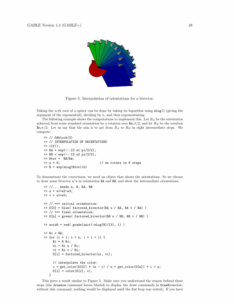
GABLE Version 1.4 (GABLE+) 28
Figure 5: Interpolation of orientations for a bivector.
Taking the n-th root of a spinor can be done by taking its logarithm using sLog() (giving theargument of the exponential), dividing by n, and then exponentiating.
The following example shows the computations to implement this. Let RA be the orientationachieved from some standard orientation by a rotation over Ie1π/2, and let RB be the rotationIe2π/2. Let us say that the aim is to get from RA to RB in eight intermediate steps. Wecompute:
>> // GAblock(3)
>> // INTERPOLATION OF ORIENTATIONS
>> clf();
>> RA = exp(-::I3 e1 pi/2/2);
>> RB = exp(-::I3 e2 pi/2/2);
>> Rtot = RB/RA;
>> n = 8; // we rotate in 8 steps
>> R = exp(sLog(Rtot)/n)
To demonstrate the correctness, we need an object that shows the orientations. So we chooseto draw some bivector u^v in orientation RA and RB, and show the intermediate orientations.
>> //... needs n, R, RA, RB
>> u = e1+e2-e3;
>> v = e1+e3;
>> // === initial orientation:
>> O[0] = blue( factored_bivector(RA u / RA, RA v / RA) )
>> // === final orientation:
>> O[n] = green( factored_bivector(RB u / RB, RB v / RB) )
>> axisR = red( grade(unit(-sLog(R)/I3), 1) )
>> Ri = RA;
>> for (i = 1; i < n; i = i + 1) {
Ri = R Ri;
ui = Ri u / Ri;
vi = Ri v / Ri;
O[i] = factored_bivector(ui, vi);
// interpolate the color:
c = get_color(O[0]) * (n - i) / n + get_color(O[n]) * i / n;
O[i] = color(O[i], c),
}
This gives a result similar to Figure 5. Make sure you understand the reason behind thesesteps (the drawnow command forces Matlab to display the draw commands in DrawBivector;without this command, nothing would be displayed until the for loop was exited). If you have

GABLE Version 1.4 (GABLE+) 29
learned about quaternions before, you may realize that the above geometric algebra approachto interpolating orientation is equivalent to unit quaternions (see also next section). For mostpeople, those are an isolated technique; you may now appreciate how they are a natural part ofthe algebraic structure of the 3-dimensional space.
Exercises
1. Verify the axis and angle in the example above by hand.
2. What happens in the example if one of the rotations, say RB , was over 180 degrees, soψ = π. Is the solution still well-behaved?
3. What happens if RA and RB occur in the same plane?
3.6 Complex numbers and quaternions: subsumed
So rotations are characterized by the plane in which they occur; those planes are characterizedby bivectors; and combinations of rotations are represented by geometric products of thesebivectors. If you have heard of complex numbers and quaternions, you know that those mayalso be used to do rotations, in the plane and in space, respectively. How does this compareto the geometric algebra method? Surprisingly, the answer is: it is exactly the same (but in aricher context)!
Algebraically, we may observe that the linear space C 3,0 has several interesting subspaceswith corresponding sub-algebras. In particular, consider the subspace spanned by {1, e1 ∧ e2}on an orthonormal basis e1, e2, e3. The product of e1 ∧ e2 with itself is
(e1 ∧ e2)(e1 ∧ e2) = e1e2e1e2 = −e1e1e2e2 = −1.
Thus in this subspace, the bivector e1 ∧ e2 has similar properties to the complex number i,and we see that indeed we can use this linear subspace of our geometric algebra spanned by 1and e1 ∧ e2 as the complex numbers, with their product represented by the geometric product(at least if we are careful about the order, due to difference in the commutative properties ofthe two algebras). Within geometric algebra, these can be seen as operators, which can act ongeometrical subspaces represented by vectors, bivectors, trivectors or scalars. Complex numberscan only multiply each other, not ‘operate’ on other objects such as vectors.
Now consider the subalgebra spanned by {1, e1 ∧ e2, e2 ∧ e3, e1 ∧ e3}. The analysis of theprevious paragraph shows that
(e1 ∧ e2)2 = (e2 ∧ e3)2 = (e1 ∧ e3)2 = −1,
Further, we have
(e1 ∧ e2)(e2 ∧ e3) = e1 ∧ e3
(e2 ∧ e3)(e1 ∧ e3) = e1 ∧ e2
(e1 ∧ e3)(e1 ∧ e2) = e2 ∧ e3
and changing the order in which we multiply these bivectors changes the sign of the result. Inother words, with the identification i = e1 ∧ e2, j = e2 ∧ e3, and k = e1 ∧ e3 we get:
i2 = j2 = k2 = −1, i j = k, j k = i, k i = j.
You may recognize this: they are the defining equations of quaternions, usually introduced as aspecial ‘number system’, somehow mysteriously handy for computations with rotations.
Now we see that the basic ‘complex numbers’ occurring in quaternions are actually a basisof bivectors in the geometric algebra C 3,0. Those seemingly imaginary numbers are actuallyreal spatial planes in disguise, and their product is just the geometric product. Not a big sur-prise, then, that quaternions are so useful in describing orientations: quaternions are actuallydisguised spinors representing the rotation planes, and their products therefore represent succes-sive rotations. Within the same framework, we can now also represent the objects on which therotations need to act, and that is a significant improvement over the quaternion representation.

GABLE Version 1.4 (GABLE+) 30
vp
p^v/vV=p^v
tangent
perpendicular support vector
moment
Figure 6: A line described by offset p and tangent v, with moment V.
3.7 Subspaces off the origin
3.7.1 Lines off the origin
You may have noticed that most of the objects we have drawn are based about the origin.Vectors start from the origin, bivectors and trivectors contain the origin. It is possible, however,to describe objects that are not centered at the origin, basically by adding a vector, bivector,etcetera to offset them to where we desire. Let’s see how.
We have already seen that a blade B characterizes a subspace through the outer product,as follows: the equation
x ∧B = 0
holds if and only if x is linearly dependent on the vectors ‘in’ the blade. So in particular, if theblade is a vector v, the equation x ∧ v = 0 characterizes the vectors of points on the line indirection v, through the origin. Its parametric solution is x = τv, for any real number τ .
To characterize a line off the origin, through a point p, we simply translate x, i.e., we letx− p satisfy the line equation. This gives
x ∧ v = p ∧ v
as the implicit equation of the line parallel to v, through p. So all points x on the line span thesame bivector with v. A line is thus implicitly characterized by a vector v (called the tangent)and a bivector V ≡ p∧v (called the moment), and determined by an arbitrary vector p on theline. These terms are illustrated in Figure 6.
This implicit characterization of the line leads to a parametric specification of the points onit, which is
x = (p ∧ v)/v + τv.
’You may recognize in the first term the rejection of p by v, i.e., the perpendicular supportvector of the line. It can also be written in terms of the moment as V/v. The variable τ is areal number; as it varies from −∞ to +∞ we obtain all points on the line.
(For those interested, here is how the parametric equation is obtained from the implicitequation x ∧ v = V. First write it as: xv = V + x · v, then divide out v to obtain: x =V/v + (x ·v)/v = V/v + (x ·v−1)v. Now recognize that x ·v−1 is a real number taking valuesbetween −∞ and +∞, effectively specifying for each point x its characterizing parameter; callit τ , and you have the parametric equation.)
So for example, if we want a line parallel to v = e2 that passes through p = e1 + e2, we areinterested in all vectors x satisfying the equation x ∧ e2 = (e1 + e2) ∧ e2 = e1 ∧ e2. Obviouslyx = e1 + τe2 is the parametric solution, and this is readily verified:
x ∧ e2 = (e1 + τe2) ∧ e2 = e1 ∧ e2 = (e1 + e2) ∧ e2,
for all real numbers τ . For example, e1 + 2e2 lies on our line. We can test this in GAViewer bychecking that the equation is satisfied:
>> (e1 + 2 e2) ^ e2 == (e1 + e2) ^ e2
ans = 1.00
We can give a graphic illustration of the bivector equality characterizing a line by using factored bivector().First draw the defining bivector for the line, i.e., its moment:

GABLE Version 1.4 (GABLE+) 31
>> a = alpha( factored_bivector(e1, e2), 0.5)
Next let’s draw the corresponding bivectors for two more pieces of the line:
>> //...
>> b = alpha( factored_bivector(e1 + e2, e2), 0.5)
>> c = alpha( factored_bivector(e1 + 2 e2, e2), 0.5)
What we see in this figure is that the gray arrows (which connect points on the line) are collinear.By varying τ in the parametric equation, we can sample points along the line. We have
written a routine called DrawPolyline() that will draw the piecewise line segment, in a ‘connectthe dots’ fashion. As arguments, DrawPolyline takes a cell array of geometric objects that areall vectors, and draws the piecewise line segment that connects the tips of these vector arguments(in Matlab, a cell array is a list of items enclosed in ‘{}’). We can use DrawPolyline to drawa portion of our line. We begin by clearing the screen and redrawing the bivector representingour line:
>> clf(); b = factored_bivector(e1+e2,e2),
Next, we draw three points and the line using point() and line(). Internally, these functionsuse the conformal model, which is not described in this tutorial. So, to draw the line x = e1+τe2:
>> //...
>> v1 = point(e1)
>> v2 = point(e1 + 3 e2)
>> v3 = point(e1 + 7 e2)
>> ln = line(v1, v2)
The three points should be collinear, as indicated pictorially by line.
3.7.2 Planes off the origin
For planes, we just use a bivector as characterizing the tangent blade B. That gives
x ∧B = p ∧B
as the equation characterizing all vectors x of points on the plane with tangent B and momentp ∧B (i.e., passing through p). We can show this graphically:
>> clf();
>> p = e1, b1 = e2, b2 = e3
>> pl1 = factored_trivector(b1, b2, p)
>> pl2 = factored_trivector(b1, b2, p + b1)
>> pl3 = factored_trivector(b1, b2, p + b2)
>> pl4 = factored_trivector(b1, b2, p + b1 + b2)
This shows pictorially that all these trivectors have a common bivector (which is b1^b2), andall the same moment; so the position vectors p, p+b1, p+b2, p+b1+b2 all lie in the same plane.Use GAorbiter() or manipulate the viewpoint using the left mouse button to see this.
You may derive that the perpendicular support vector is now (p ∧B)/B.The parametric equation of the plane involves two scalar parameters (this is a slightly more
advanced subject; read the rest of this section only if you are interested). Let B = b1 ∧ b2
with b1 and b2 orthogonal so that we may even write B = b1b2, then starting from theparametric equation derived similarly to that of the line, we rewrite using the inner productidentity x · (b1b2) = (x · b1)b2 − (x · b2)b1 (which is equation 13):
x = (x ∧B)/B + (x ·B)/B
= (p ∧B)/B + (x ·B)/B
= (p ∧B)/B + (x · (b1b2))B−1
= (p ∧B)/B + ((x · b1)b2 − (x · b2)b1) B−1
= (p ∧B)/B + (x · b1)b2B−1 − (x · b2)b1B
−1
= (p ∧B)/B + (x · b1)b−11 + (x · b2)b−1
2
= (p ∧B)/B + (x · b−11 )b1 + (x · b−1
2 )b2
= (p ∧B)/B + τ1b1 + τ2b2,
with the appropriate definitions of τ1 ≡ (x · b−11 ) and τ2 ≡ (bx · b−1
2 ).

GABLE Version 1.4 (GABLE+) 32
pV
p
qU
v
u
vu q
Figure 7: Intersection of two lines.
3.7.3 Intersection of two lines
Suppose we have two lines in a plane (but not through the origin) and we wish to find theirintersection. For example, as illustrated in the left half of Figure 7, suppose we have the twolines described by
x ∧ u = p ∧ u
x ∧ v = q ∧ v
In this figure, we draw p and q emanating from the origin, and u and v emanating from theheads of p and q respectively to indicate the direction of the lines.
Rearranging to get the diagram on the right half of this figure, we see that the intersectionis given by U + V, where U and V are scaled versions of u and v respectively. What we needto find are the two scale factors. But from the figure, we see that the scale factor needed toscale u to U is given by the ratio of the area of the parallelogram defined by U and v (which isq ∧ v) to the area of the parallelogram defined by u and v (which is u ∧ v). These quantitiesthus come immediately from the outer product, and we using the symmetric construction to getthe scale factor for V, we see that the intersection is given by
q ∧ v
u ∧ vu +
p ∧ u
v ∧ uv. (17)
Note here that the outer products in each ratio are bivectors whose area is the area of theparallelogram spanned by the two vectors. When we divide a bivector by a parallel bivector,the bivector parts cancel, leaving only the ratio of the two scalar components. Here is anexample of application of Equation 17:
// GAblock(4)
// LINE INTERSECTS LINE
>> clf();
>> p = e2, u = 0.2 e2 + e1;
>> q = e1, v = e2 - 2 e1;
>> p1 = p - 2u; p2 = p + 2u;
>> line1 = blue(line(p1, p2))
>> q1 = q - 2v; q2 = q + 2v;
>> line2 = green(line(q1, q2))
In this diagram, we have drawn two lines, one in blue and one in green. Now draw
>> //...
>> U = magenta( (q ^ v / u ^ v) u )
>> V = magenta( (p ^ u / v ^ u) v )
>> i = U + V
Here we see the magenta vectors are scaled versions of the u and v directions of the lines. Thesum of the magenta vectors is the red vector, which points to the intersection point of the twolines.

GABLE Version 1.4 (GABLE+) 33
Exercises
1. Intersect the line x ∧ (e1 + 2e2) = 0 with the line x ∧ (e2 − e1) = (e1 + e2) ∧ (e2 − e1).Draw a picture similar to the one above.
2. What happens to the above intersection code if one of the lines passes through the origin(e.g., p=0;)? Does it still work? Why or why not?
3. What happens to the above intersection code if the lines are parallel (i.e., u = v)? Trythis in GAViewer. Later we will see line intersection code that does not have this problem.
4. As a guess for the formula specifying the intersection point of a line x ∧ u = p ∧ u and aplane x ∧V = q ∧V (where V is the bivector tangent of the plane), try:
q ∧V
u ∧Vu +
p ∧ u
V ∧ uV
on some examples. Did it work? Can you see why, geometrically?
3.8 Summary
In this section, we have studied geometric computations. Using the three products, we haveseen how to compute projections, rejections, reflections and rotations. We also looked at linesoff the plane, and saw how to use the geometric operations to intersect these lines.
4 Blades and subspace relationships
Blades are the fundamental objects in geometric algebra. We have seen how a k-blade is formedby taking the outer product of k independent vectors. We have also shown that a blade representsa k-dimensional subspace containing the origin. In the next section, we present a trick to makeblades represent subspaces off-set from the origin. That obviously makes blades very relevantobjects in geometric algebra, and their geometry worthy of a separate study.
In this section, we determine the operations required to assess the relative positions of blades:how they project onto each other, how they can be decomposed relative to each other, and howthey intersect. This intersection will necessitate the definition of a new kind of product ingeometric algebra, the meet, and a related product, the join, as geometric union.
4.1 Subspaces as blades
Picture, in your mind, two blades; they can be a vector and a bivector, two vectors, two bivectors,or they may even be scalars (blades of grade 0). As you visualize them in the way we have done,you actually make each of those k-blades characterize a k-dimensional subspace, through theequivalence
vector x in subspace determined by A ⇔ x ∧A = 0.
This interpretation of blades is not specific on sign or magnitude of A, so by themselves,subspaces have no significant sign or magnitude. For now, we can think of subspaces as ‘bladesmodulo a multiplicative scalar’ – but we’ll keep in mind that geometric algebra would allow usto be more quantitative about subspaces than we may have been used to. By the way, note thata scalar blade A yields the equation x = 0, so that it represents a point at the origin.
We would like to encode the following relationships of subspaces into geometric algebra:
• projection of subspaces onto each other, and its counterpart: rejection of subspaces by eachother
• intersection of subspaces, including how ‘orthogonal’ this intersection is
• ‘union’ of subspaces: common span, or common superspace, with some measure of theirdegree of parallelness
• the ‘sides’ of a space split by a subspace
• a distance measure between subspaces
We will see that a limited set of operators can express all these concepts, and that they arecomposed of the products we have defined so far.
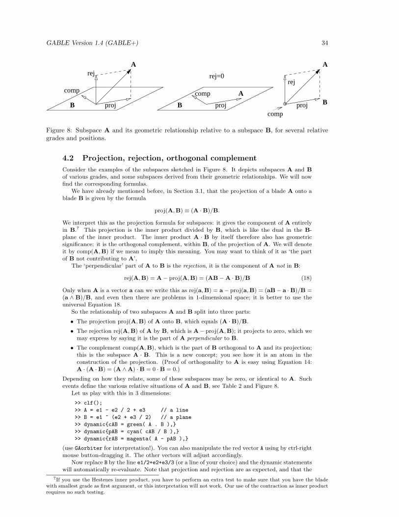
GABLE Version 1.4 (GABLE+) 34
B proj
A
A
B proj
rej=0
A
Bproj
rej
comp
compcomp
rej
Figure 8: Subspace A and its geometric relationship relative to a subspace B, for several relativegrades and positions.
4.2 Projection, rejection, orthogonal complement
Consider the examples of the subspaces sketched in Figure 8. It depicts subspaces A and Bof various grades, and some subspaces derived from their geometric relationships. We will nowfind the corresponding formulas.
We have already mentioned before, in Section 3.1, that the projection of a blade A onto ablade B is given by the formula
proj(A,B) ≡ (A ·B)/B.
We interpret this as the projection formula for subspaces: it gives the component of A entirelyin B.7 This projection is the inner product divided by B, which is like the dual in the B-plane of the inner product. The inner product A · B by itself therefore also has geometricsignificance: it is the orthogonal complement, within B, of the projection of A. We will denoteit by comp(A,B) if we mean to imply this meaning. You may want to think of it as ‘the partof B not contributing to A’,
The ‘perpendicular’ part of A to B is the rejection, it is the component of A not in B:
rej(A,B) = A− proj(A,B) = (AB−A ·B)/B (18)
Only when A is a vector a can we write this as rej(a,B) = a− proj(a,B) = (aB− a ·B)/B =(a ∧ B)/B, and even then there are problems in 1-dimensional space; it is better to use theuniversal Equation 18.
So the relationship of two subspaces A and B split into three parts:
• The projection proj(A,B) of A onto B, which equals (A ·B)/B.
• The rejection rej(A,B) of A by B, which is A− proj(A,B); it projects to zero, which wemay express by saying it is the part of A perpendicular to B.
• The complement comp(A,B), which is the part of B orthogonal to A and its projection;this is the subspace A · B. This is a new concept; you see how it is an atom in theconstruction of the projection. (Proof of orthogonality to A is easy using Equation 14:A · (A ·B) = (A ∧A) ·B = 0 ·B = 0.)
Depending on how they relate, some of these subspaces may be zero, or identical to A. Suchevents define the various relative situations of A and B, see Table 2 and Figure 8.
Let us play with this in 3 dimensions:
>> clf();
>> A = e1 - e2 / 2 + e3 // a line
>> B = e1 ^ (e2 + e3 / 2) // a plane
>> dynamic{cAB = green( A . B ),}
>> dynamic{pAB = cyan( cAB / B ),}
>> dynamic{rAB = magenta( A - pAB ),}
(use GAorbiter for interpretation!). You can also manipulate the red vector A using by ctrl-rightmouse button-dragging it. The other vectors will adjust accordingly.
Now replace B by the line e1/2+e2+e3/3 (or a line of your choice) and the dynamic statementswill automatically re-evaluate. Note that projection and rejection are as expected, and that the
7If you use the Hestenes inner product, you have to perform an extra test to make sure that you have the bladewith smallest grade as first argument, or this interpretation will not work. Our use of the contraction as inner productrequires no such testing.

GABLE Version 1.4 (GABLE+) 35
projection rejection ‘complement’proj(A,B) rej(A,A) comp(A,B) description
= (A ·B)/B = A− (A ·B)/B A ·Bscalar 0 `-blade A is a scalark-blade 0 (`− k)-blade A lies in Bk-blade 0 scalar A and B coincidek-blade k-blade (`− k)-blade ` 6= k: in general positionk-blade k-blade scalar non-trivial intersection
0 k-blade 0 A perpendicular to B
Table 2: Relationship between two subspaces A (of grade k) and B (of grade ` ≥ k).
orthogonal complement to A in B is now a scalar. The point at the origin is indeed the onlysubspace of B and ‘orthogonal’ to both A and its projection.
Now do the same on two non-identical planes, for instance A = e2^(e1+e3) and B = e1^(e2+e3/2),and interpret the results. (As you may see, the magnitudes of the bivectors are somewhat diffi-cult to interpret using the automatic drawing command. We’ll soon use factored bivector()
instead, but then we first need to find the intersection of the planes, to span them nicely.)This subspace interpretation casts an interesting new light on the inner product of vectors.
We have seen that a scalar is, geometrically, the representation of a point at the origin. The innerproduct u ·v of two vectors u and v is the subspace of v which is the orthogonal complement ofu; and geometrically, that is the point at the origin, on the line determined by v. So the innerproduct of two vectors is a weighted point...
If you want to stretch your intuition for generalization to new limits, use the space itself forB, so take B = I3 and take A to be a line, and then a plane. Verify what you see by computation!Why does the dual subspace appear? Can you make yourself see and feel that the rejection ofA from 3-space is 0, which is ‘not even a point’?
The same formulas and interpretation are still applicable when A and B are coincident spaces:play around with B = 2*A, choosing a line, plane or I3 for A. What is the projection now?
What you may learn from all this is that geometric algebra has no special cases for computingsuch geometric relationships. It is not always easy to find the characterization in words of whatis computed since it may not be a classically recognized concept (our notion of ‘orthogonalcomplement of A in B’ is a bit of a stretch), but we have found it rewarding to add theoutcomes of straightforward computations as a elementary concepts to our intuition.
4.3 Angles and distances
A vector x has several relevant relationships with respect to a planar or linear subspace A in3-space such as its incidence angle, the distance of its tip to the subspace, and the ‘side’ it lieson. With projection and rejection, these are easy to compute.
• perpendicular distanceThe perpendicular distance is obviously the length of the rejection |(rej(x,A))| = |(x− (x ·A)/A)| =|((x ∧A)/A)|.
• sideThe quantity x ∧A is the space spanned by x and A; we can compare this to the bladewe might already have for this subspace to determine whether x lies on the ‘positive’ or‘negative’ side of A. If A is a 2-blade, then x ∧ A is a 3-blade (or zero, in which casex lies in A). So we can compute the side as the sign of the scalar (x ∧ A)/I3. If A isone-dimensional, there is no natural orientation to give to the 2-blade x ∧A: so a line in3-space has no sides (for a point – it does induce a sense in lines).
Note that the side is closely related to the perpendicular distance: for the plane we canwrite I3 = nA, with n the normal vector of A (so that n ·A = 0). Then (x ∧A)I−1
3 =(x ∧ A)/A/n = rej(x,A)/n. Since the rejection and n are parallel, this is a scalar,expressing the perpendicular distance in units of n (if you take x = n, you get 1). So fora point relative to a plane, we obtain a signed distance, and that is often more useful thanjust the absolute value of the perpendicular distance.

GABLE Version 1.4 (GABLE+) 36
• angleThe angle of a vector relative to a line or plane is characterized by the ratio between itsrejection and projection, which is like the tangent function from trigonometry:
rej(x,A)
proj(x,A)=
x ∧A
x ·A .
The magnitudes of x and A cancel, so it is properly independent of scale. Note that wehave not taken norms, so that the result is a bivector (it is the ratio of a (k+1)-blade and a(k− 1)-blade, so a 2-blade). We may write the outcome as i tanφ. This explicitly gives usthe plane i in which the angle is to be measured, and it cancels the bothersome ambiguityof sign which the use of a tangent always involves. The above expression computes i tanφ,and if you wished to interpret the angle in the oppositely oriented plane −i, the value ofthe tangent function (and therefore the angle φ) automatically changes sign. As we haveseen when treating rotations, angles are essentially bivectors! (It is even possible to extendthe trigonometric functions naturally to geometric algebra; then the formula may be saidto compute tan(iφ), see [9]).
Let us try this out:
// GAblock(5)
// PROJECTION, REJECTION
clf();
x = blue( e1 + e2/2 + e3 ),
A = green( e2 + e3/3 ),
pxA = magenta( (x . A) / A ),
rxA = magenta( (x ^ A) / A ),
p_plus_r = pxA + rxA; // projection + rejection
cmd("fgcolor black");
cmd("polygon line1 3 pxA p_plus_r rxA dm2");
distxA = norm(rxA),
tanglexA = rxA/pxA;
anglexA = atan(norm(tanglexA))*180/pi,
B = yellow( e1^A ), // A planar subspace (containing A)
pxB = red( (x . B) / B ),
rxB = red( (x ^ B) / B ),
p_plus_r2 = pxB + rxB;
cmd("polygon line2 3 pxB p_plus_r2 rxB dm2");
distxB = norm(rxB),
tanglexB = rxB/pxB;
anglexB = atan(norm(tanglexB))*180/pi,
Exercises
1. What do you get if you compute these quantities relative to a 0-dimensional subspaceA = 2, or relative to the total 3-space A = I3? Can you interpret those outcomessensibly?
2. If you add ‘1’ to the bivector we computed above, you get an operator which (under post-multiplication) rotates and scales x to be in the subspace A. Why? Check this for thesubspaces in the GAViewer example above.
3. In 3-dimensional space, the relative orientation of two planes is also determined by anangle. Can you give a formula for the value of its tangent function?
4.4 Intersection and union of subspaces: meet and join
In the example of the two planes:

GABLE Version 1.4 (GABLE+) 37
>> // GAblock(6)
>> // MEET, JOIN
>> clf();
>> A = blue( e2 ^ (e1 + e3) ),
>> B = green( e1 ^ (e2 + e3 / 3) ),
>> cAB = A . B,
>> pAB = cyan( cAB / B ),
>> rAB = magenta( A - pAB ),
we see that the formulas so far do not determine their line of intersection. Such an intersectionbetween subspaces is obviously something we often need; so we need to make it computational.
First, how do we determine that a subspace A has a non-trivial intersection with subspaceB? In such a case, there is at least a 1-dimensional subspace c in common. Rewriting theblades in the form A = A′ ∧ c and B = c ∧ B′, we see that A ∧ B = (A′ ∧ c) ∧ (c ∧ B′) =A′ ∧ (c ∧ c) ∧B′ = A′ ∧ 0 ∧B′ = 0. So we find:
A and B have non-trivial intersection ⇔ A ∧B = 0.
Of course the fact that A ∧B = 0 may mean that there are several independent 1-dimensionalsubspaces in common; A and B might even coincide completely. Let us suppose that C is alargest common subspace of A and B (in the sense of: the highest dimensionality, so the highestgrade). Then we can write A = A′ ∧C and B = C ∧ B′, so we can ‘factor out’ the commonsubspace C. (The weird order is to get better signs later on.)
The common subspace C is the ‘intersection’ of the two subspaces A and B. We would liketo define an operation in geometric algebra that produces it; let us call that the meet operation.It is thus defined by:
If A and B can be factored using a highest grade sub-blade C as A = A′∧C and B =C ∧B′, then their meet is meet(A,B) = C.
We have indeed implemented such an operation:
>> //... needs A,B
>> mAB = meet(A,B) // this is equal to mAB = A & B
However, you should be somewhat careful with using its outcome. The problem is that thefactorization is not unique, and so neither is the meet. Since C is a blade indicating a subspace,any multiple γC is just as valid, and that would produce a meet of γC. We could demand|C| = 1 (at least in Euclidean spaces), but that would still leave the sign undetermined. Theoutcome of the meet is therefore a strange ‘object’: it has no well-defined sign. Its meaning asa subspace is perfectly clear (x is in C iff x ∧C = 0), but as a blade it is ambiguous: it has nounique orientation that can be established on the basis of A and B alone.
If we consider C in the context of the superspace spanned by A and B, we can be morespecific on its orientation. This common superspace is like a union of the spaces A and B. Itis often called the join of A and B, and we define it through the factorization we had before:
If A and B can be factored using a highest grade sub-blade C as A = A′∧C and B =C ∧B, then their join is: join(A,B) = A′ ∧C ∧B′ (= A′ ∧B = A ∧B′).
This we have also implemented:
>> //... needs A,B
>> jAB = join(A,B) // this is equal to jAB = A | B
Obviously, in this case of two distinct 2-blades in 3-space, it is proportional to I3. If A and Bwould be disjoint, then join(A,B) is proportional to A ∧B.
Again, the problem is that the factorization is not unique, and replacing C by γC nowchanges the join by a factor of 1/γ. Thus we have the problem of assigning a magnitude to thejoin, as we did for the meet. Although we have no mechanism in geometric algebra to fix themagnitudes uniquely (and this is a fundamental impossibility, since it is the ambiguity of thefactorization that causes it), we can at least make a meet and join that are consistent, in thesense that they are based on the same factorization. This can be done based on the observationthat join and meet are related by
join(A,B) =A
meet(A,B)∧B.

GABLE Version 1.4 (GABLE+) 38
(A derivation may be found in [15, 16].) It can be rewritten to the more commonly seen form
meet(A,B) =B
join(A,B)·A.
We have moreover scaled the meet to have unit norm. This fixes meet and join up to one sharedambiguous sign.
4.5 Combining subspaces: examples
With projection, rejection, orthogonal complement, meet and join, we have a powerful set ofterms to describe many (all?) relationships between subspaces. And they are all computationallyrelated, we can use their properties both synthetically to construct new objects reflecting therelationships, or analytically in derivations.
Let us play around with these new tools. We have written a small function drawall() thatdraws the all these geometric relationships in one go: [[ wouldn’t it be better to make it abatch, so that we don’t need to explain about the ::? ]]
batch drawall(e3ga A, e3ga B) {
drawall_obj1 = blue( A ),
drawall_obj2 = green( B ),
drawall_comp = red( lcont(A, B) ),
drawall_proj = cyan( ::da_comp / B );
drawall_rej = magenta( A - ::drawall_proj );
drawall_meet = black( A & B ),
drawall_join = yellow( A | B ),
}
Note the colors used to draw objects, and realize that if objects overlap exactly, one of themmay not be visible. It is therefore a good idea to use non-unit-norm blades for A and B, so thatthe various objects are more likely to have different magnitudes.
Let us first continue the example of the two intersecting planes A and B of Section 4.2.Remember how it was hard to see whether the projection was done correctly when we drew thebivectors using the standard method? We can use the above functions to redo that quickly:
>> clf();
>> drawall(e2 ^ (e1+e3), e1 ^ (e2+e3/2))
Now that we have the meet operation, we can use the meet as a common vector in the two planes,and this permits us to use factored bivector() to show the various blades more clearly in afactored form.
>> // GAblock(7)
>> // MEET AND JOIN DECOMPOSED
>> clf();
>> A = e2^(e1+e3);
>> B = e1^(e2+e3/2);
>> M = black( 0.5 A & B ), // scale with 0.5 for clearer drawings
>> // draw A decomposed:
>> fA = blue( factored_bivector(A / M, M) )
>> // draw B decomposed:
>> fB = green( factored_bivector(M,1/M * B) )
>> // draw projection decomposed:
>> fP = cyan( factored_bivector(project(A, B) / M, M) )
>> // draw rejection decomposed:
>> fR = magenta( factored_bivector((A - project(A, B)) / M, M) )
>> // draw the join:
>> J = yellow(A | B)

GABLE Version 1.4 (GABLE+) 39
You now see how the magnitudes of projection and rejection obviously give the original A astheir sum, which was hard to appreciate in the circular way of drawing the bivectors.
What we have defined is general for blades of any dimension. For instance, let’s take a1-blade and a 2-blade.
>> clf();
>> drawall(e1-e2/2+e3, e1^(e2+e3/2));
The fact that the meet is a scalar, indicates that the intersection is the point a the origin.Or take a 0-blade and a 1-blade, a rather degenerate case:
>> drawall(3, 2 (e2 + e3));
No matter how degenerate the situation, our relationship operators have no exceptions,and the results are always sensibly interpretable. These functions and operators are extremelystable to any blades you might use them on, and they can be used to implement all of classicalgeometry.
One more step is needed: to show how blades can represent off-set subspaces such as linesand planes in general position. The old GABLE used to have a part on the homogenous modelright here, but we decided to leave that out and to refer to our tutorial on conformal geometricalgebra tutorial instead, where it is treated in a better context.
Exercises
1. The vector p = e1 + e2 lies in the plane A = (e1 + e2) ∧ e3 (as you may verify). Howfar does its endpoint lie from the intersection of A with the plane B = 2(e1 ∧ (e2 + e3)?Draw this!
2. What is the angle between p and the intersection of A and B?
5 Is this all there is?
Our tutorial stops here. We have familiarized you with the basic operators that geometricalgebra offers, and some of their geometrical significance. The intuition acquired should enableyou to read some of the other texts which are available, and get you into the right mode ofthinking in geometrical concepts.
There are some things we left out of the tutorial. Since they are rather elementary, you mayrun into them soon after trying other texts, so a few words may be appropriate.
• signatures3-dimensional space can be given different signatures, so that the unit vectors do not squareto 1, but to another scalar such as −1. We have chosen not to confuse the novice withthe strange properties of non-Euclidean spaces, but GAViewer contains two non-Euclideanalgebras:
– c3ga: 5D geometric algebra for use with conformal model of 3D euclidean space.
– i2ga: an experimental 6D geometric algebra for operations on 2.5 Dimages.
.
• inner productsThere are several inner products around; the one we have chosen is by no means standard,though it has the most straightforward geometric interpretation. The most common intexts is the one introduced by Hestenes, which we have coded as hip(). You can playaround with the other inner products through inner product():
>> inner_product(lcont); // set the . operator to left contration
>> inner_product(rcont); // set the . operator to right contration
>> inner_product(hip); // set the . operator to Hestenes inner product
>> inner_product(mhip); // set the . operator to modified Hestenes inner product
• higher dimensionsIn this tutorial, we have only used 3-dimensional geometric algebra. However, GAVieweralso contains a 4D algebra for use with the homogeneous model, a 5D algebra for use withthe conformal model, and 6D algebra for images.

GABLE Version 1.4 (GABLE+) 40
• other models of Euclidean geometry; other geometriesA natural follow-up to this material is our tutorial on the conformal model of Euclideangeometry, which uses GAViewer to good effect. It will appear soon on our site. We recom-mend it to show how far the GA thinking can go to make effective models of computation.Yet the model is still rather fresh, and you don’t need it immediately (but you’re gonnalove it!).
• differential geometryA major subject we have not treated is differential geometry, and geometric calculus. Theobjects in geometric algebra can be differentiated, in new and powerful ways, and thisis beginning to expand the scope of all fields using differential geometry. Matlab is lesssuited to show this flexibly. The Maple implementation of geometric algebra written inCambridge [10] is a good tool to use when studying these new forms of differentiation (forinstance combined with their course [3]).
Further reading
To deepen your understanding after our introduction, we’d like to recommend some literaturefor further study. When you look around on the web, you’ll find that many people are enthusias-tically writing down their own first understanding of the material. This may be very helpful toyou (it often spells out details that more experienced texts leave out), but you may risk missingthe point of it all, since the methods and style of thinking tends to be pre-GA. So our recom-mendations are for more mature texts (ahem). Some of these are from the physics community,where it has been used slightly longer. But increasingly, computer science applications can alsobe found.
We would recommmend the following material.
• The first part of the two part CG&A tutorial [5, 14] is mostly covered by this tutorial; thesecond part takes it further into more advanced topics.
• Our tutorial on CGA (conformal geometric algebra), when it appears, is a natural followupin the same style. Then read the third CG&A part [6] on five ways to do ray tracing.
• The introductory chapters of ‘New Foundations of Classical Mechanics’ [9].
• The general chapters of ‘Geometric Algebra for Physicists’ [4].
• An application to a basic but involved geometry problem in computer vision, with a briefintroduction into geometric algebra [11].
• Papers showing how linear algebra becomes enriched by viewing it as a part of geometricalgebra [2, 8].
Read them in approximately this order. We are working on texts more specifically suited for acomputer graphics audience; these may first appear as SIGGRAPH courses.
You can also find a large amount of additional literature from the usual sources. However,one warning: some people make no distinction between ‘geometric algebra’ and ‘Clifford algebra’so you may want to check both; but you will find that the literature on the latter contains littlebasic geometry (it tends to be about spinors). Your best keyword for initial search is ‘geometricalgebra’. readable to non-physicists. There is no standard journal to follow the developmentsin GA, and that is as it should be: when all is said and done, geometric algebra is merely a toolto do interesting geometrical things, so the uses should appear in the technical journals of eachfield.
If you got interested in the software aspects, there are various toolkits available for Matlab,Maple, Mathematica and the like, and these are helpful to your study though they do not reallyhave production speeds. Many neglect the visualization of GA, which we find so helpful todevelop our thinking. If you want to write a bigger application, look at our C++ implementationGaigen (which is behind GAViewer), which we have used to build a ray tracer and some otherapplications. Other fast software is Clifford and CLU. But all attempts are the basic geometry,there are no packages yet with a lot of algorithms from computational geometry (such as Voronoidiagrams, convex hull, and the like). Our website should have up-to-date links to availablepackages and their properties.
In de bibl plakken en XXX maken....

GABLE Version 1.4 (GABLE+) 41
A GAViewer details
Details on GAViewer can be found in its manual [7].
B Glossary
This glossary is meant to convey the geometric flavor of terms, rather than their exact definitions– for those the reader is referred to the appropriate sections.
• Bivector - A directed area element, a 2-dimensional direction. Formed by the outer productof two independent vectors, it determines a plane through the origin. (Section 2.2.2)
• Blade - a subspace through the origin; a k-blade is constructed as the outer product of kvectors. (Section 2.2.7)
• Dual - The orthogonal complement of a multivector (usually a blade); made throughdivision by the unit volume. (Section 2.4.3)
• Geometric product - The product to scale, rotate and orthogonalize multivectors; it pro-vides a geometric operator. (Section 2.4.1)
• Grade involution - take the k-blade A and multiply it by (−1)k; for multivectors, do thisfor each of its blades. (Section 2.5)
• Homogeneous model - The embedding of n-dimensional Euclidean space in an (n + 1)-dimensional geometric algebra.
• Inner product - the product used when orthogonal complements are involved. (Section 2.3)
• Inverse - The inverse under the geometric product; denoted by A−1 (as object) or by /A(as right-side operator). (Section 2.4.2)
• Multi-vector - a sum of blades, the most general element of geometric algebra. (Sec-tion 2.2.7)
• Outer product - The product used for spanning subspaces. (Section 2.2)
• Projection - The component of a blade totally contained in another blade; or the operationproducing this. (Section 3.1)
• Pseudoscalar - The outer product of all the vectors in a basis for our vector space; the‘volume-element’ of the space. (Section 2.2.3)
• Rejection - The component of a blade totally outside another blade; or the operationproducing this. (Section 3.1)
• Spinor - a product of vectors, to be used as the operator S in the spinor product SxS−1.(Section 3.4.2)
• Trivector - A directed volume element. Formed by the outer product of three independentvectors. (Section 2.2.3)
• Vector - The basic 1-dimensional elements of a linear space spanning a geometric space.A basis for this vector space generates the linear space of the geometric algebra of thegeometric space.
• Wedge product - Another name for the outer product. (Section 2.2)
References
[1] Chin-Liang Chang and Richard Char-Tung Lee. Symbolic logic and mechanical theoremproving. Academic Press, 1973.
[2] C Doran, A Lasenby, and S Gull. Linear algebra. In WE Baylis, editor, Clifford (Geo-metric) Algebras with Applications in Physics, Mathematics and Engineering, chapter 6.Birkhauser, 1996.
[3] Chris Doran and Anthony Lasenby. Physical applications of geometric algebra. Availableat http://www.mrao.cam.ac.uk/~clifford/ptIIIcourse/, 1999.
[4] C. Doran, A. Lasenby, ‘Geometric Algebra for Physicists’, Cambridge University Press,2003, ISBN 0 521 48022 1

GABLE Version 1.4 (GABLE+) 42
[5] Leo Dorst and Stephen Mann. Geometric algebra: a computation framework for geometricalapplications: Part i. Computer Graphics and Applications, 22(3):24–31, May/June 2002.
[6] D. Fontijne, L. Dorst, Modelling 3D Euclidean Geometry, IEEE CGA, March/April 2003,pp. 68-78.
[7] D. Fontijne, L. Dorst, T. Bouma and S. Mann. GAViewer: Interactive Geometric Algebrawith OpenGL visualization, Available at http://www.science.uva.nl/ga/viewer/, 2003.
[8] David Hestenes. The design of linear algebra and geometry. Acta Applicandae Mathemat-icae, 23:25–63, 1991.
[9] David Hestenes. New Foundations for Classical Mechanics. Reidel, 2nd edition, 2000.
[10] Anthony Lasenby et al. GA package for Maple V.Available at http://www.mrao.cam.ac.uk/~clifford/software/GA/, 1999.
[11] J. Lasenby, W J Fitzgerald, C J L Doran, and A N Lasenby. New geometric methods forcomputer vision. International Journal of Computer Vision, 36(3):191–213, 1998.
[12] Hongbo Li, David Hestenes, and Alyn Rockwood. Generalized homogeneous coordinatesfor computational geometry. Springer Series in Information Science. To be published 1999.
[13] Pertti Lounesto, Risto Mikkola, and Vesa Vierros. CLICAL user manual: Complex number,vector space and clifford algebra calculator for MS-DOS personal computers. TechnicalReport Institute of Mathematics Research Reports A248, Helsinki University of Technology,1987.
[14] Stephen Mann and Leo Dorst. Geometric algebra: a computation framework for geometricalapplications: Part ii. Computer Graphics and Applications, 22(4):58–67, July/August 2002.
[15] Stephen Mann, Leo Dorst, and Tim Bouma. The making of a geometric algebra packagein Matlab. Technical Report CS-99-27, University of Waterloo, December 1999. Availableas ftp://cs-archive.uwaterloo.ca/cs-archive/CS-99-27/.
[16] Stephen Mann, Leo Dorst, and Tim Bouma. The making of GABLE, a geometric algebralearning environment in Matlab. In E. Bayro-Corrochano and G. Sobczyk, editors, Geo-metric Algebra with Applications in Science and Engineering, pages 491–511. Birkhauser,2001.
[17] David Wells. The Penguin Dictionary of Curious and Interesting Geometry. Penguin, 1991.