G89.2247 Lect 3 1

G89.2247Lecture 3

• Review of mediation

• Moderation

• SEM Model notation

• Estimating SEM models

G89.2247 Lect 3 2

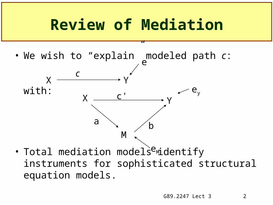
Review of Mediation

• We wish to “explain” modeled path c:

with:

• Total mediation models identify instruments for sophisticated structural equation models.

Yey

X

M

c'

b

eM

a

Xc

e

Y

G89.2247 Lect 3 3

Nonrecursive models

• All the models we have considered are recursive. The causal effects move from one side of the diagram to the other.

• A Nonrecursive model has loops or feedback.

X1 Y1

X2 Y2

e1

e2

G89.2247 Lect 3 4

Example

• Let X1 be college aspirations of parents of adolescent 1 and X2 be aspiration of parents of adolescent 2.

• Youth 1 aspirations (Y1) are affected by their parents and their best friend (Y2), and Youth 2 has the reciprocal pattern.

• This model is identified because it assumes that the effect of X1 on Y2 is completely mediated by Y1.

• Special estimation methods are needed. OLS no longer works.

G89.2247 Lect 3 5

Moderation

• Baron and Kenny (1986) make it clear that mediation is not the only way to think of causal stages

• A treatment Z may enable an effect of X on YFor Z=1 X has effect on YFor Z=0 X has no effect on Y

• When effect of X varies with level of Z we say the effect is Moderated

• SEM methods do not naturally incorporate moderation models

G89.2247 Lect 3 6

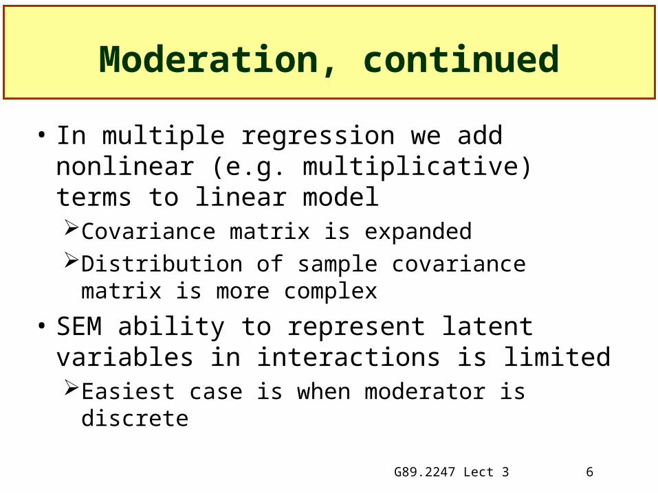
Moderation, continued

• In multiple regression we add nonlinear (e.g. multiplicative) terms to linear modelCovariance matrix is expandedDistribution of sample covariance matrix is more

complex

• SEM ability to represent latent variables in interactions is limitedEasiest case is when moderator is discrete

G89.2247 Lect 3 7

• Suppose that X is perceived efficacy of a participant and Y is a measure of influence at a later time. Suppose S is a measure of perceived status. Perceived status might moderate the effect of efficacy on influence.

• Two ways to show this:

• Equation: Y=b0+b1X+b2S+b3(X*S)+e

Path Diagrams of Moderation

X

S

Y

e

For S low:

For S high:

X Y

e

X Y

e

(+)

+ +

G89.2247 Lect 3 8

SEM and OLS Regression

• SEM models and multiple regression often lead to the same resultsWhen variables are all manifestWhen models are recursive

• The challenges of interpreting direct and indirect paths are the same in SEM and OLS multiple regression

• SEM estimates parameters by fitting the covariance matrix of both IVs and DVs

G89.2247 Lect 3 9

SEM Notation for LISREL (Joreskog)

• Lisrel's notation is used by authors such as Bollen

Y2

Y1

X1

2

11

2

1

2

1

12

1

1

0

00

XY

Y

Y

Y

XYBY

G89.2247 Lect 3 10

SEM Notation for EQS (Bentler)

• EQS does not name coefficients. It also does not distinguish between exogenous and endogenous variables.

E

V3

V2

V1

E

G89.2247 Lect 3 11

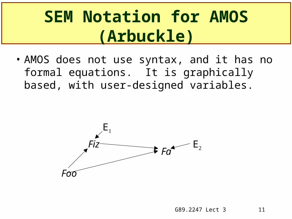
SEM Notation for AMOS (Arbuckle)

• AMOS does not use syntax, and it has no formal equations. It is graphically based, with user-designed variables.

E

FaFiz

Foo

E

G89.2247 Lect 3 12

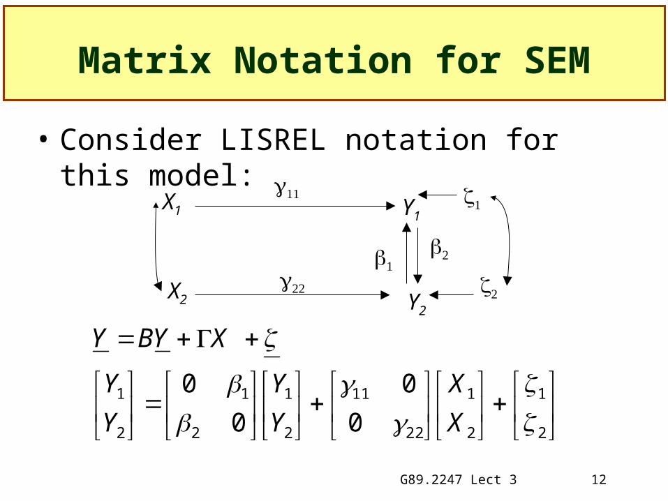
Matrix Notation for SEM

• Consider LISREL notation for this model:

Y2

Y1

X2

2

1

2

1

22

11

2

1

2

1

2

1

0

0

0

0

X

X

Y

Y

Y

Y

XYBY

X1

G89.2247 Lect 3 13

More Matrix Notation

• The matrix formulation also requires that the variance/covariance of X be specifiedSometimes is used, sometimes XX.

• The variance/covariance of is also specifiedConventionally this is called .

• When designing structural models, the elements of and can either be estimated or fixed to some (assumed) constants.

G89.2247 Lect 3 14

Basic estimation strategy

• Compute sample variance covariance matrix of all variables in modelCall this S

• Determine which elements of model are fixed and which are to be estimated. Arrange the parameters to be estimated in vector .Depending on which values of are assumed, the fitted

covariance matrix () has different values

• Choose values of that make the S and as close as possible according using a fitting rule

G89.2247 Lect 3 15

Estimates Require Identified Model

• An underidentified model is one that has more parameters than pieces of relevant information in S.The model should always have

where t is the number of parameters, p is the number of Y variables and q is the number of X variables

Necessary but not sufficient condition

2/1 qpqpt

G89.2247 Lect 3 16

Other identification rules

• Recursive models will be identified• Bollen and others describe formal

identification rules for nonrecursive models• Rules involve expressing parameters as a

function of elements of S.• Informal evidence can be obtained from

checking if estimation routine convergesHowever, a model may not converge because of

empirical problems, or poor start values

G89.2247 Lect 3 17

Review of Expectations

• The multivariate expectationsVar(X + k*1) = Var(k* X) = k2

• Let CT be a matrix of constants. CT X=W are linear combinations of the X's.

Var(W) = CT Var(X) C = CT C • This is a matrix

G89.2247 Lect 3 18

Multivariate Expectations

• In the multivariate case Var(X) is a matrixV(X)=E[(X-) (X-)T]

24434241

34233231

24232221

14131221

G89.2247 Lect 3 19

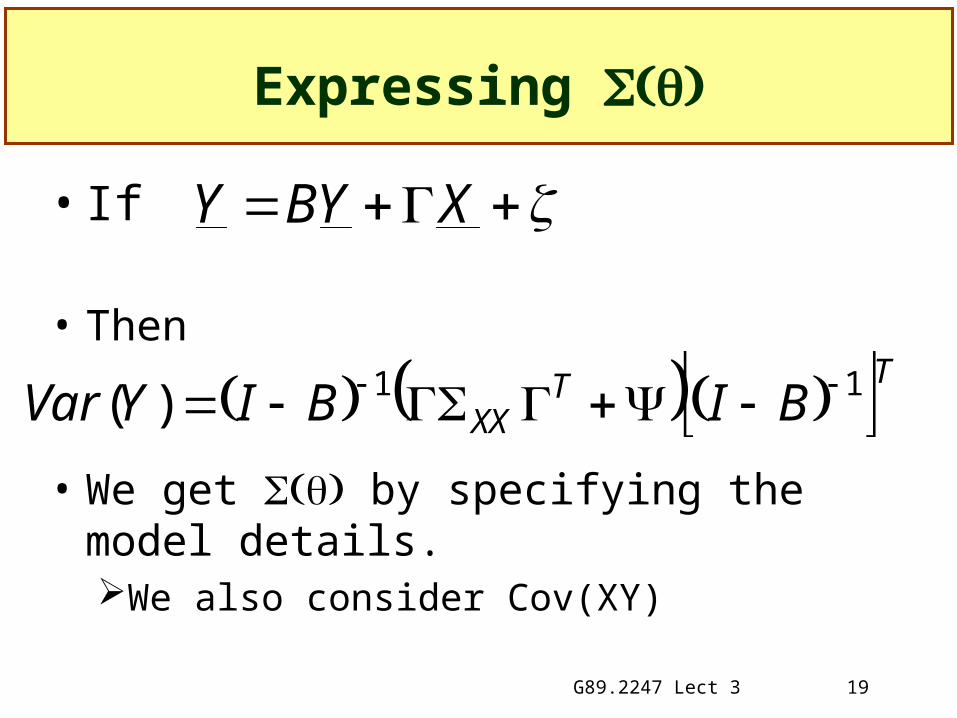
Expressing

• If

• Then

• We get by specifying the model details.We also consider Cov(XY)

XYBY

TTXX BIBIYVar 11)(

G89.2247 Lect 3 20

Estimation Fitting Functions

• ML minimizes

• ULS minimizes

• GLS minimizes

1lnln)( StrSF

SStrF

11 SSSStrF

G89.2247 Lect 3 21

Excel Example

B

0 0 0.6798 0 0.99226 0.54831 0.64895 0.11614 B 00.3939 0 0 0.4646 0.54831 1.15378 0.11614 0.65445 B 0.3939

0.6798S X1 X2 Y1 Y2 0.4646X1 1.0452 0.5004 0.6356 0.5204 ML= 0.0762 LR= 18.9762 0.99226X2 0.5004 1.1538 0.4433 0.6829 ULS= 0.0204 1.15378Y1 0.6356 0.4433 1.1075 0.7256 GLS= 0.0503 LR= 12.5176 0.54831Y2 0.5204 0.6829 0.7256 1.3033 0.64895

N= 250 0.654450.99226 0.54831 0.67454 0.52045 0.116140.54831 1.15378 0.37274 0.682870.67454 0.37274 1.1075 0.725560.52045 0.68287 0.72556 1.30326 Y1= 0 Y2+ 0.6798 X1+ 0 X2+E1

S- Y2= 0.39 Y1+ 0 X1+ 0.4646 X2+E20.053 -0.048 -0.039 0.000-0.048 0.000 0.071 0.000-0.039 0.071 0.000 0.0000.000 0.000 0.000 0.000

G89.2247 Lect 3 22

Choosing between methods

• ML and GLS are scale freeResults in inches can be transformed to results in feetULS is not scale free

• All methods are consistent• ML technically assumes multivariate normality, but it

actually is related to GLS, which does not• Parameter estimates are less problematic than standard

error estimates