G ra viton propa gat or - Max Planck Societyloops05.aei.mpg.de/index_files/PDF_Files/rovelli.pdf ·...
23
Graviton propagator Carlo Rovelli LOOPS05, Potsdam October 2005
Transcript of G ra viton propa gat or - Max Planck Societyloops05.aei.mpg.de/index_files/PDF_Files/rovelli.pdf ·...
Graviton propagator
Carlo Rovelli
LOOPS05, Potsdam October 2005

carlo rovelli graviton propagator 2
• General approach to background-independent QFT
• Kinematics well-defined:+ Separable kinematical Hilbert space (spin networks, s-knots)+ Geometrical interpretation (area and volume operators)- Euclidean/Lorentzian ? Immirzi parameter ?
• Dynamics:
• Thiemann’s operator (with its variants and ambiguities)• Spinfoam formalism (several models)- triangulation independence:
Group Field Theory (+ good finiteness, - λ ?)Conrady-Bojowald-Perez triangulation invariance ?
- Barrett-Crane vertex, or 10j symbol
Where we are in LQG
Avertex ∼ eiSRegge + e−iSRegge + D
Barrett, Williams, Baez, Christensen, Egan, Freidel, Louapre
badgood
carlo rovelli graviton propagator 3
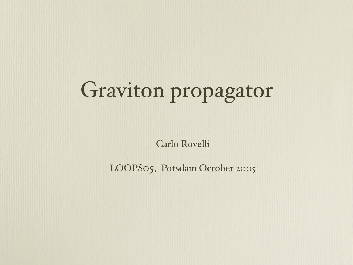
Developments• Matter fields• Mathematical formalization (uniqueness theorem)
Applications• Spectra of Area and Volume• Loop cosmology• Black hole entropy• Black hole singularity• Astrophysical• ...
Main open issues• Which version is the good one?• Low energy limit• Newton’s law• Computing scattering amplitudes This talk

carlo rovelli graviton propagator 4
W (x, y) =
∫Dφ φ(x) φ(y) eiS[φ]
W (x, y) = W (f(x), f(y))
The problem
if measure and action are diff invariant, then immediately
W [ϕ, Σ] =
∫φint|Σ=ϕ
Dφint eiS[φint]
W (x, y; Σ, Ψ) =
∫Dϕ ϕ(x) ϕ(y) W (ϕ, Σ) Ψ[ϕ]
Idea for a solution: define the boundary functional
φint
ϕ
Σ•
•
x
y
then
cfr: R Oeckl (see also Conrady, Doplicher)
carlo rovelli graviton propagator 5
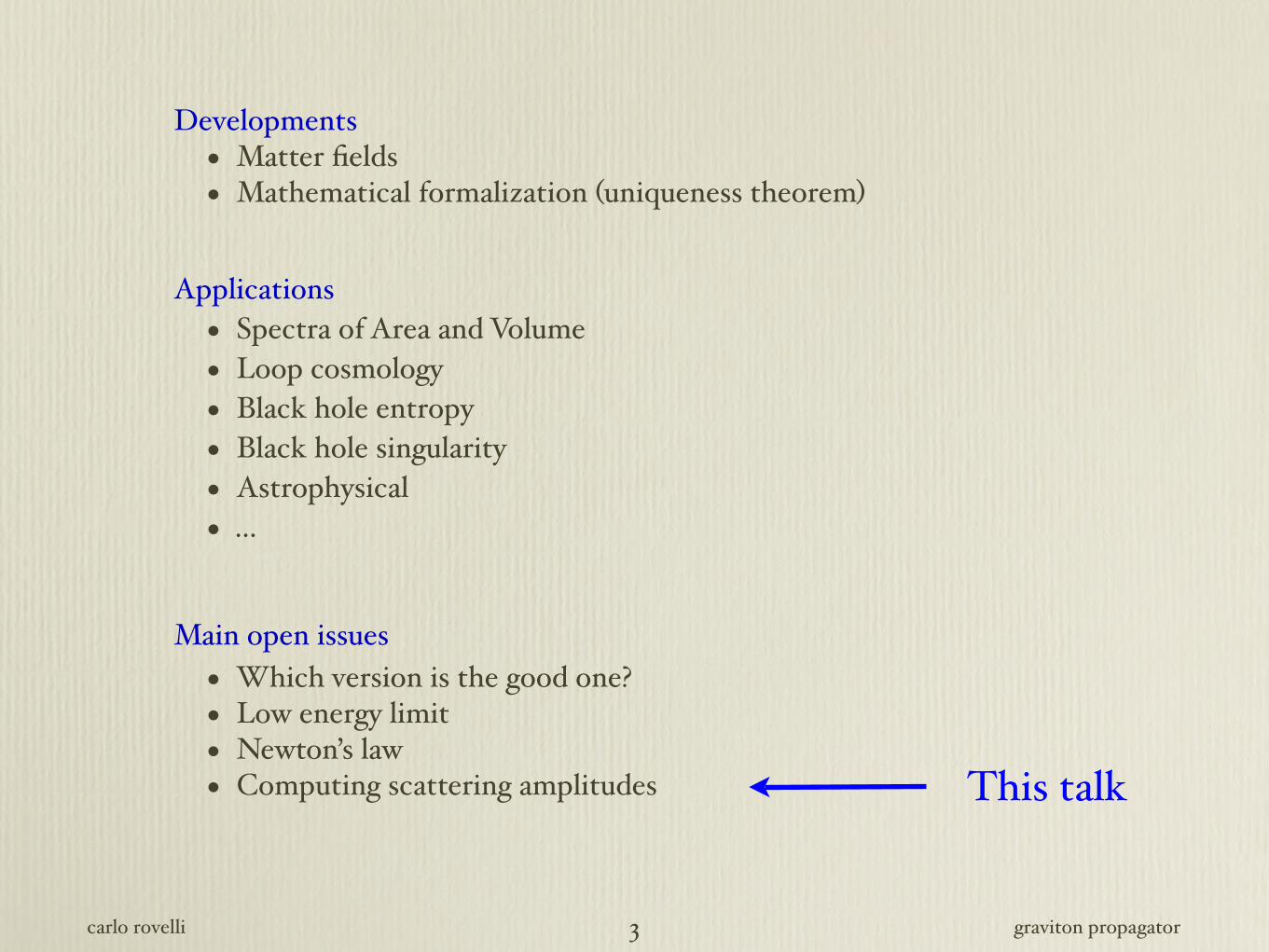
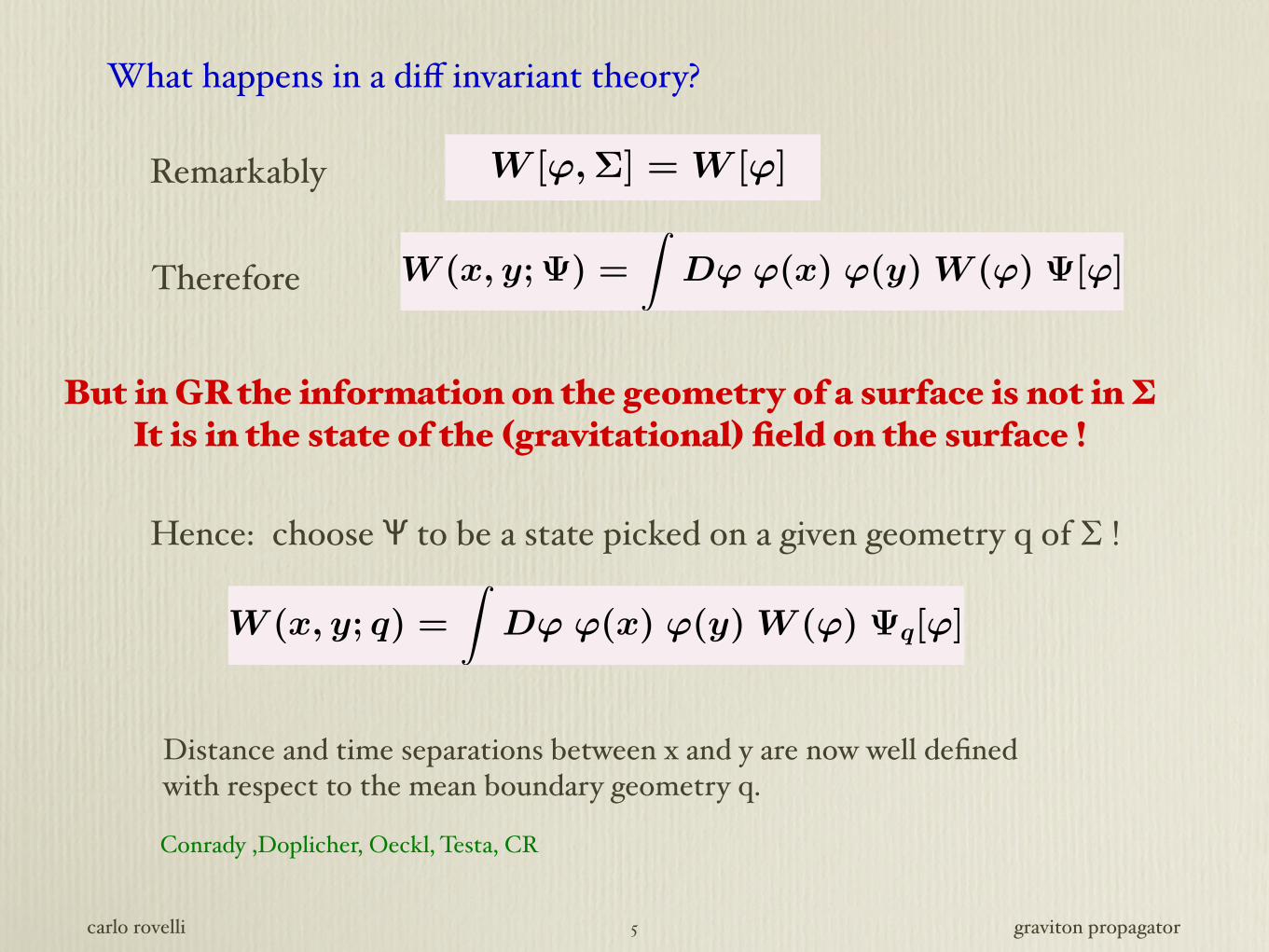
What happens in a diff invariant theory?
W [ϕ, Σ] = W [ϕ]Remarkably
W (x, y; Ψ) =
∫Dϕ ϕ(x) ϕ(y) W (ϕ) Ψ[ϕ]Therefore
But in GR the information on the geometry of a surface is not in ∑It is in the state of the (gravitational) field on the surface !
Hence: choose Ψ to be a state picked on a given geometry q of ∑ !
W (x, y; q) =
∫Dϕ ϕ(x) ϕ(y) W (ϕ) Ψq[ϕ]
Distance and time separations between x and y are now well defined with respect to the mean boundary geometry q.
Conrady ,Doplicher, Oeckl, Testa, CR
carlo rovelli graviton propagator 6
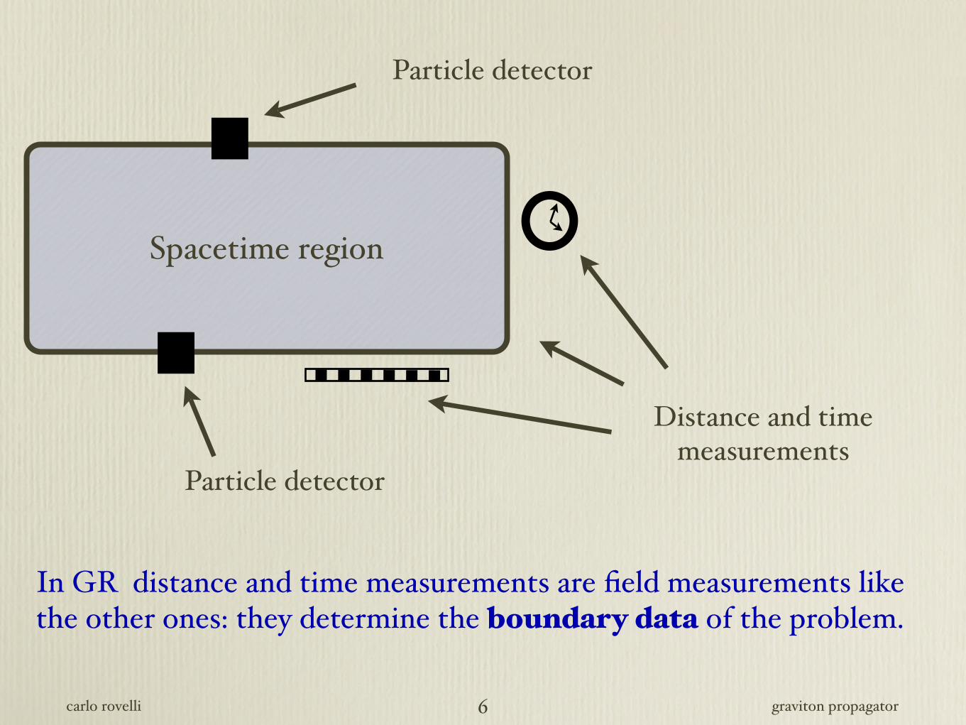
Spacetime region
Particle detector
Particle detector
Distance and time measurements
In GR distance and time measurements are field measurements like the other ones: they determine the boundary data of the problem.

carlo rovelli graviton propagator 7
Give meaning to the expression φint
•
•
x
y(∑, q)
• ∫Dφ ∑s-knots
• W [φ] W [s] defined by GFT spinfoam model
• Ψq a suitable coherent state on the geometry q
• φ(x) graviton field operator from LQG.
W (x, y; q) =
∫Dϕ ϕ(x) ϕ(y) W [ϕ] Ψq[ϕ]
W abcd(x, y; q) = N∑ss′
W [s′] 〈s′|hab(x)hcd(y)|s〉 Ψq[s]
Modesto, CR, PRL 05

W [s] =
∫Dφ fs(φ) e− ∫
φ2− λ5!
∫φ5
W [s] =∑
∂σ=s
∏faces
Afaces
∏vertices
Avertex
W (3g) =
∫∂g=3g
Dg eiSEinstein−Hilbert[g]
carlo rovelli graviton propagator 8
W [s] : Group field theory (here GFT/B):
The Feynman expansion in λ gives a sum over spinfoams
which has a nice interpretation as a discretization of the Misner-Hawking sum over geometries
with background triangulations summed over as well.

W [s] =λ
5!
( ∏n<m
dim(jnm)
)Avertex(jnm)
!
!!!
! !!!!!!!!!
""
""
"""#
##
##
##
$$$$$$$$$
%%%%%
&&
&&
'''''''''
''''%
%%%%%%%
((
(((
))
))
)))
**
**
***
s =
j12
j23
j34
j45
j51
j13
j35
j14j24
j52
carlo rovelli graviton propagator 9
To first order in λ, the only nonvanishing connected term in W[s] is for
And the dominant contribution for large j is given by the spinfoam σ dual to a single four-simplex. This is

Ψq[s] = exp
{−α
2
∑n<m
(jnm − j(0)nm)2 + i
∑n<m
Φ(0)nmjnm
}
carlo rovelli graviton propagator 10
The boundary state Ψq(s)
• Choose a boundary geometry q: let q be the geometry of the 3d boundary (∑,q) of a spherical 4d ball, with linear size L >> √ħG.
• Interpret s as the (dual) of a triangulation of this geometry. Choose a regular triangulation of (∑, q); interpret the spins as the areas of the corresponding triangles, using the standard LQG interpretation of spin networks.
• This determine the “background” spins j(0)nm=jL. Ψq(s) must be picked on these values. Choose a Gaussian state around these values with with α, to be determined.
• A Gaussian can have an arbitrary phase:
Ψq(s) must be a coherent state, determined by coordinate and momentum, namely by intrinsic 3-geometry and extrinsic 3-geometry q !!
The Φ (0)nm = Φ are the background dihedral angles.

carlo rovelli graviton propagator 11
L
j12
ϕ12

EIi(n)EIi (n)|s〉 = (8π!G)2 jI(jI + 1)|s〉
hab(!x) = gab(!x) − δab = Eai(!x)Ebi(!x) − δab
W (L) = W abcd(x, y; q) nanbmcmd
carlo rovelli graviton propagator 12
The field operator
Choose x to be on the nodes and contract the indices with two parallel vectors along the links. Then we have the standard action on boundary spin networks, well known from LQG
!
!!!
! !!!!!!!!!
""
""
"""#
##
##
##
$$$$$$$$$
%%%%%
&&
&&
'''''''''
''''%
%%%%%%%
((
(((
))
))
)))
**
**
***
j12
j23
j34
j45
j51
j13
j35
j14j24
j52
x
y
n
m
Define
W (L) = i8π
4π2
1
|x − y|2q= i
8π!G
4π2
1
L2
Standard perturbative theory gives( )

carlo rovelli graviton propagator 13
x
y
n
m

carlo rovelli graviton propagator 14
The expression for the propagator is then well defined:
Nλ(!G)4
5!
∑jnm
(j12(j12 + 1) − j2L) (j34(j34 + 1) − j2
L) Avertex(jnm) e−α2
∑n,m(jnm−jL)2−iΦ
∑n,m jnm
rapidly oscillating phaseAvertex ∼ eiSRegge + e−iSRegge + D
W (L) = W abcd(x, y; q)nanbmcmd =
only the “good” component of Avertex survives !
This is the “forward propagating” (Oriti, Livine) component of Avertex cfr. Colosi, CR
SRegge(jnm) =∑n<m
Φnm(j) jnmBut sinceSRegge(jnm) ∼ Φ
∑nm
jnm +1
2G(mn)(kl)δjmnδjkland

Where is the (“discrete”) derivative of the dihedral angle, with respect to the area (the spin).
It can be computed from geometry, giving , where k is a numerical factor ~ l
SRegge(jnm) ∼ Φ∑nm
jnm +1
2G(mn)(kl)δjmnδjkl
G(mn)(kl) =∂Φmn(jij)
∂jkl
∣∣∣∣jij=jL
carlo rovelli graviton propagator 15
G(mn)(kl)
G(12)(34) =8π!Gk
L2
W (L) =4i
α2G(12)(34)
The gaussian “integration” gives finally

carlo rovelli graviton propagator 16
Φ12

carlo rovelli graviton propagator 17
Φ12
A34=8πħG j34

carlo rovelli graviton propagator 18
Φ12
A34=8πħG j34

carlo rovelli graviton propagator 19
Φ12
A34=8πħG j34
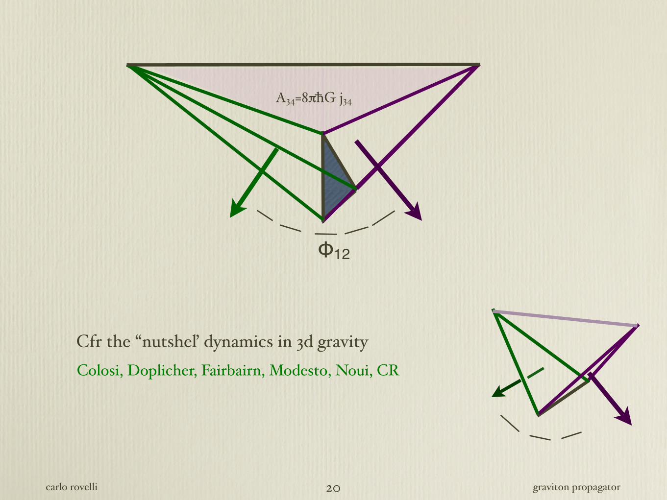
Colosi, Doplicher, Fairbairn, Modesto, Noui, CR
Cfr the “nutsheľ dynamics in 3d gravity
carlo rovelli graviton propagator 20
Φ12
A34=8πħG j34
Colosi, Doplicher, Fairbairn, Modesto, Noui, CR
Cfr the “nutsheľ dynamics in 3d gravity
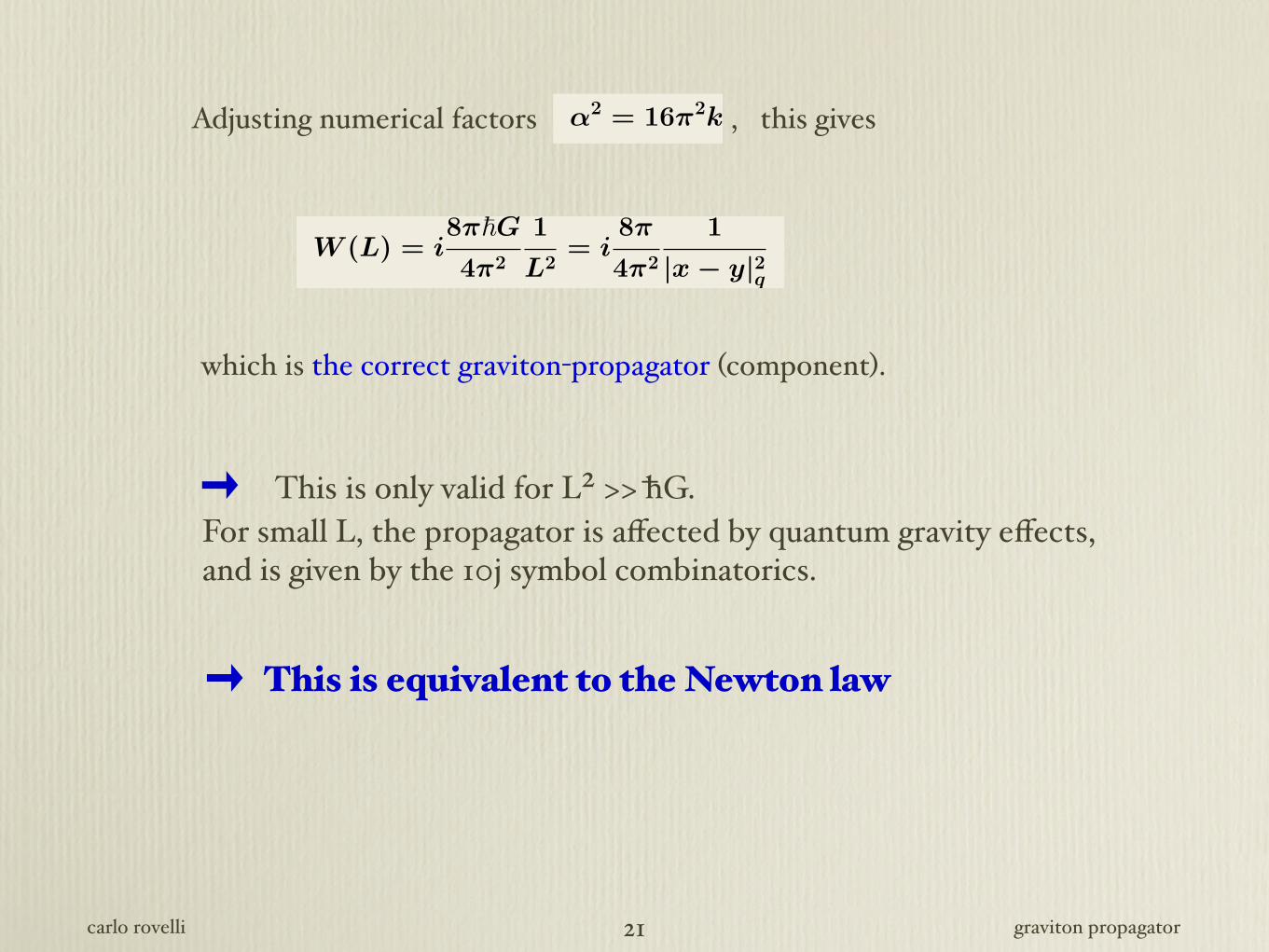
α2 = 16π2k
W (L) = i8π!G
4π2
1
L2= i
8π
4π2
1
|x − y|2q
carlo rovelli graviton propagator 21
Adjusting numerical factors , this gives
which is the correct graviton-propagator (component).
This is only valid for L2 >> ħG. For small L, the propagator is affected by quantum gravity effects, and is given by the 10j symbol combinatorics.
This is equivalent to the Newton law

carlo rovelli graviton propagator 22
• Is it just by chance?
• Other components? Full tensorial structure (Modesto, Speziale) (intertwiners)
• Do higher order terms in λ change the result ? (Modesto)
• Other models (GFT/C seems to give the same result (Modesto))
• n - point functions ? Computing the undetermined constants of the non-renormalizable perturbative QFT ?
• ...
Open issues

carlo rovelli graviton propagator 23
i. Low energy limit. (One component of) the graviton propagator (or the Newton law) appears to be correct, to first order in λ.
ii. Barret-Crane vertex. Only the “good” component of the 10j symbol survives, because of the phase of the state, given by the extrinsic geometry of the boundary state. The BC vertex works.
iii. Scattering amplitudes. A technique to compute n-point functions within a background-independent formalism exists.
Conclusion