Godel’s System T Revisited

Sandra Alves a, Maribel Fernandez b,Mario Florido a and Ian Mackie c

a LIACC - University of Porto,R. do Campo Alegre 1021/1055, 4169-007, Porto, PortugalbKing’s College London, Department of Computer Science,

Strand, London WC2R 2LS, U.K.cLIX, CNRS UMR 7161, Ecole Polytechnique, 91128 Palaiseau Cedex, France

Abstract

The linear lambda calculus, where variables are restricted to occur in terms exactlyonce, has a very weak expressive power: in particular, all functions terminate inlinear time. In this paper we consider a simple extension with natural numbers anda restricted iterator: only closed linear functions can be iterated. We show propertiesof this linear version of Godel’s System T using a closed reduction strategy, andstudy the class of functions that can be represented. Surprisingly, this linear calculusoffers a huge increase in expressive power over previous linear versions of System T ,which are ‘closed at construction’ rather than ‘closed at reduction’. We show thata linear System T with closed reduction is as powerful as System T .

1 Introduction

One of the many strands of work stemming from linear logic [16] is the area oflinear functional programming languages (see, for instance, [1,29,23]). Theselanguages are based on a version of the λ-calculus with a type system cor-responding to intuitionistic linear logic, and provide explicit syntactical con-structs for copying and erasing terms (corresponding to the exponentials inlinear logic).

A question that arises from this work is what exactly is the computationalpower of a linear calculus without the exponentials, i.e., a calculus that is syn-tactically linear: all variables occur exactly once. This is a severely restrictedform of the (simply typed) λ-calculus: computation is defined by the usualβ-reduction rule, but since there is no duplication or erasing of terms during

Preprint submitted to Elsevier 10 September 2009

reduction, this calculus has a very limited computational power — it can beshown that all functions terminate in linear time [21].

In this paper, we build this language up by introducing pairs, and naturalnumbers with the corresponding iterator, to obtain a linear version of Godel’sSystem T which we shall call System L. System T is an extension of the simplytyped λ-calculus with numbers and a recursion operator. It is a very simplesystem, yet has an enormous expressive power. We will show that its powercomes essentially from primitive recursion combined with linear higher-orderfunctions — we can achieve the same power in a calculus that has just thesetwo ingredients: System L.

In a correctness proof for the Geometry of Interaction [17], Girard uses a strat-egy for cut elimination where cut elimination steps can only take place whenthe exponential boxes are closed. Not only is this strategy for cut elimina-tion simpler than the general one, it is also exceptionally efficient in terms ofthe number of cut elimination steps. Translations of the λ-calculus into linearlogic inspired the work on closed reduction strategies in the λ-calculus [12,13].Closed reductions avoid α-conversion but (in contrast with standard weakstrategies) allow reductions inside abstractions, achieving more sharing of com-putation. We use a closed reduction strategy in System L, thus, iterators onopen linear functions are accepted (since these terms are linear), but they areonly reduced after the function becomes closed: reduction preserves linearity.

This design choice, which departs from previous linear versions of System T(see for instance [11,22]), has an enormous impact in the computation power ofthe calculus: System L is as powerful as System T . Usual definitions of linearsystems, which require iterator terms to be built using closed functions, arestrictly less powerful than System T [11,22]. We analyse the interplay betweenlinearity, iteration and closed reduction in Godel’s System T as follows:

(1) We show that a closed reduction strategy is adequate for the evaluationof programs in System T . For this, we define a version of System T ,called Tc, where reduction can only take place when certain argumentsare closed, and show that Tc is equivalent to T . We also define a system T0where iterators are syntactically restricted so that only closed functionscan be used, and show that also T0 is equivalent to T . In other words,neither closed reduction nor closed construction restrictions affect SystemT ’s computational power.

(2) We then introduce linearity constraints in System T , together with aclosed reduction strategy. We show that this linear version of System T(System L) also has the computational power of the full System T . Inother words, linearity does not affect the computational power of SystemT if we use a closed reduction strategy for iterators.

(3) To compare the closed reduction and closed construction approaches, we

2

define two linear versions of System T with a restricted product type.In the first one, which we call LN

0 , iterator terms can only be built usingclosed functions. System LN

0 can only encode primitive recursive func-tions, unlike T0 and L which are as powerful as System T . The secondsystem, called LN, uses a closed reduction strategy to reduce iteratorterms and can encode non-primitive recursive functions, such as Acker-mann’s function.

Related work. Linearity may be defined in three main ways: syntactical,operational and denotational. Operational linearity means that redexes cannotbe duplicated during evaluation (cf. weak linear terms in [5] and simple termsin [24]). Denotational linearity is achieved when only linear functions canbe defined in the language [14,32] (note that denotational linear terms mayuse variables non-linearly). Finally, syntactical linearity requires a linear useof variables in terms, and it is the computational counterpart of linearityin linear logic. The language defined in [32] is a linear version of PCF in adenotational sense: it has a linear model (linear coherence spaces) but its termscan contain more than one occurrence of the same variable. In this paper, wepresent syntactically linear versions of System T , where terms contain exactlyone occurrence of each variable.

A number of calculi, many based on linear logic, have been designed with theaim of capturing specific complexity classes (see, for instance, [6,15,20,7,26,34,8]).Bounded linear logic [20] is an interesting example: it has a computationalpower that lies in-between the linear and the full λ-calculus; specifically, it cap-tures the polynomial time computable functions. There is also previous workthat uses linear types to characterise computations with time bounds [22].Thus our work can be seen as establishing another calculus with good compu-tational properties which does not need the full power of the exponentials, andintroduces the non-linear features (copying and erasing) through alternativemeans.

From a categorical perspective, it is well-known that a Cartesian closed cat-egory (CCC) models the structure of the simply typed λ-calculus (i.e., theλ-calculus is the internal language for CCC [27,28]). The internal language ofa symmetric monoidal closed category (SMCC) is the linear λ-calculus [30].If we add a natural numbers object (NNO) to this category, then this cor-responds to adding natural numbers and an iterator to the calculus. In thissetting, a question that arises is therefore: what is the correspondence betweenCCC and SMCC+NNO? Although this is not the focus of the present paper,it is indeed a motivation for following this line of investigation.

3

Overview. In the next section, we recall the background material. Section 3defines a version of System T with closed reduction, called Tc, and comparesit with T0, which uses the ’closed-at-construction’ approach to iteration. Themain result here is that T = T0 = Tc. System L is defined in Section 4 byimposing linearity constraints in System T , together with a closed reductionstrategy. In Section 5, we demonstrate that we can encode the primitive re-cursive functions in this calculus, and even go considerably beyond this classof functions. In Section 6, we show how to encode Godel’s System T , andin Section 7 we analyse the power of linear systems with and without closedreduction. Finally we conclude the paper in Section 8. This paper is a revisedand extended version of [3,4]. For more detailed proofs and examples we referto [2].

2 Background

We assume the reader is familiar with the λ-calculus [9]. In this section werecall the main notions from Godel’s System T , for more details see [19].

System T is the simply typed λ-calculus (with arrow types, written A → B,and products A×B, and the usual β-reduction and projection rules) where abasic type N for numbers and a recursor have been added. Numbers are builtfrom 0 and S; we write n or Sn 0 for S . . . (S︸ ︷︷ ︸

n

0), and in general tnu will denote

n applications of t to u. The recursor is defined by the reduction rules:

R 0 u v −→ u

R (S t) u v −→ v (R t u v) t

Figure 1 shows the entire system. Typing contexts are sets of assumptions ofthe form x:A, where x is a variable and A is a type, such that there is at mostone assumption for each variable. We denote by dom(Γ) the set of variablesxi such that xi:Ai ∈ Γ, and write Γ, x:A to denote the “update” of Γ withx:A; more precisely, Γ, x:A is the typing context obtained by adding the typeassumption x:A in Γ, if x 6∈ dom(Γ), or by replacing the type assumption forx with x:A, if x ∈ dom(Γ).

System T is confluent, strongly normalising and reduction preserves types [19].

Our first step towards building a linear version of System T will be to replacethe recursor by a simpler iterator:

iter 0 u v −→ u iter (S t) u v −→ v(iter t u v)

4

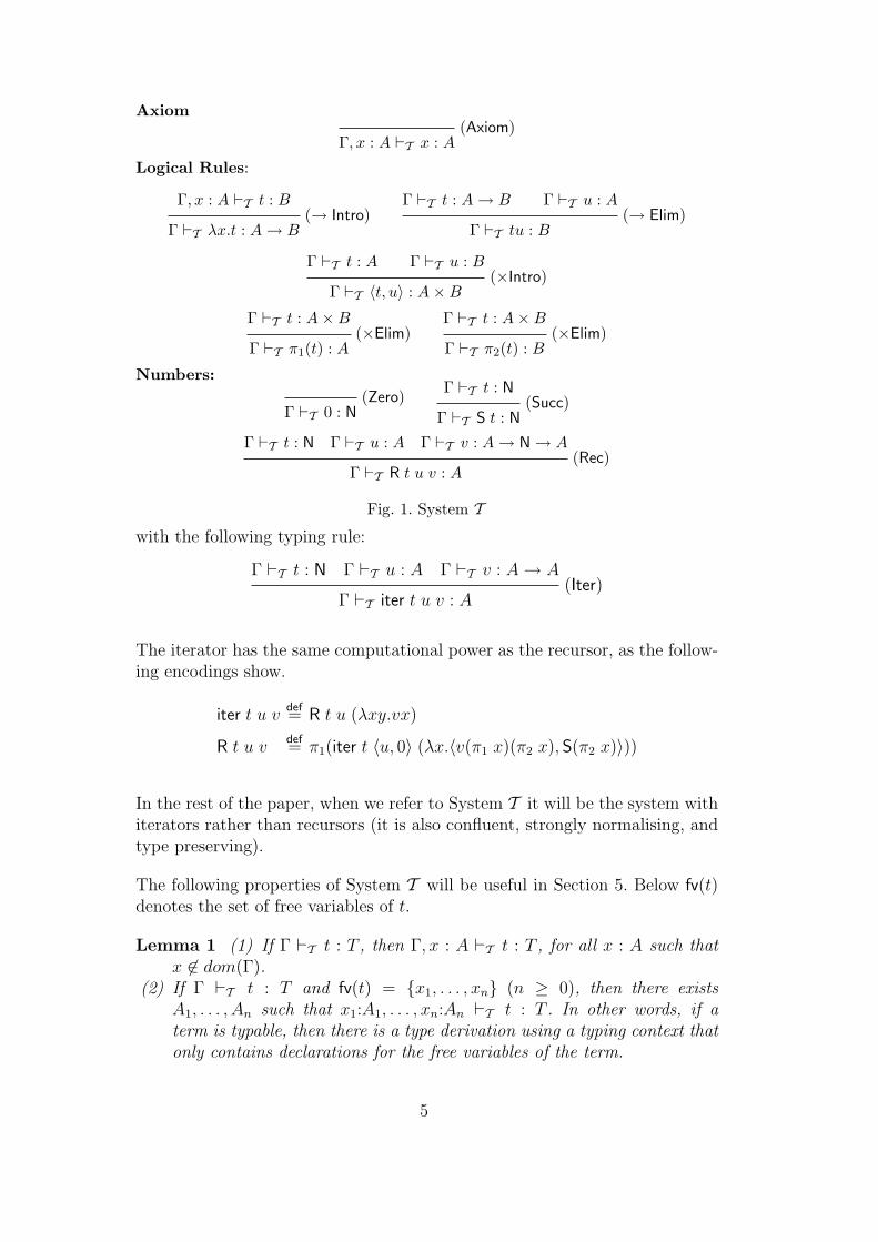
Axiom(Axiom)

Γ, x : A `T x : A

Logical Rules:

Γ, x : A `T t : B(→ Intro)

Γ `T λx.t : A→ B

Γ `T t : A→ B Γ `T u : A(→ Elim)

Γ `T tu : B

Γ `T t : A Γ `T u : B(×Intro)

Γ `T 〈t, u〉 : A×BΓ `T t : A×B

(×Elim)Γ `T π1(t) : A

Γ `T t : A×B(×Elim)

Γ `T π2(t) : B

Numbers:(Zero)

Γ `T 0 : N

Γ `T t : N(Succ)

Γ `T S t : N

Γ `T t : N Γ `T u : A Γ `T v : A→ N→ A(Rec)

Γ `T R t u v : A

Fig. 1. System T

with the following typing rule:

Γ `T t : N Γ `T u : A Γ `T v : A→ A(Iter)

Γ `T iter t u v : A

The iterator has the same computational power as the recursor, as the follow-ing encodings show.

iter t u vdef= R t u (λxy.vx)

R t u vdef= π1(iter t 〈u, 0〉 (λx.〈v(π1 x)(π2 x), S(π2 x)〉))

In the rest of the paper, when we refer to System T it will be the system withiterators rather than recursors (it is also confluent, strongly normalising, andtype preserving).

The following properties of System T will be useful in Section 5. Below fv(t)denotes the set of free variables of t.

Lemma 1 (1) If Γ `T t : T , then Γ, x : A `T t : T , for all x : A such thatx 6∈ dom(Γ).

(2) If Γ `T t : T and fv(t) = x1, . . . , xn (n ≥ 0), then there existsA1, . . . , An such that x1:A1, . . . , xn:An `T t : T . In other words, if aterm is typable, then there is a type derivation using a typing context thatonly contains declarations for the free variables of the term.

5

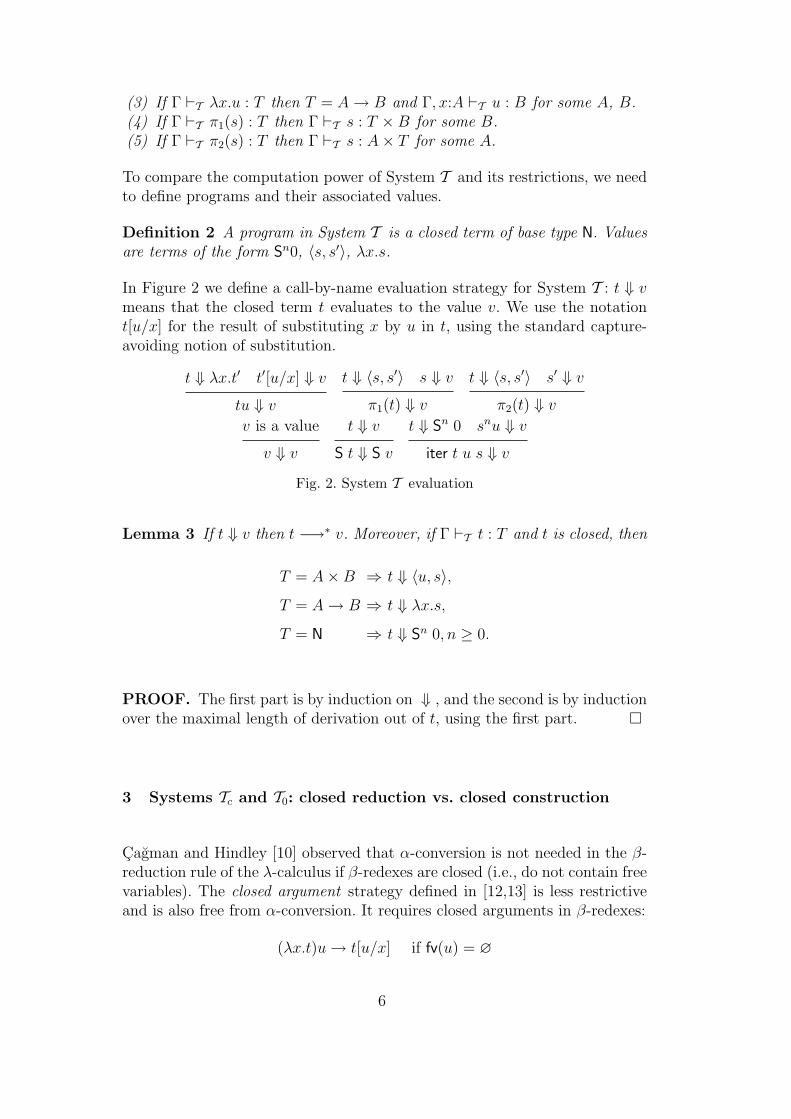
(3) If Γ `T λx.u : T then T = A→ B and Γ, x:A `T u : B for some A, B.(4) If Γ `T π1(s) : T then Γ `T s : T ×B for some B.(5) If Γ `T π2(s) : T then Γ `T s : A× T for some A.

To compare the computation power of System T and its restrictions, we needto define programs and their associated values.

Definition 2 A program in System T is a closed term of base type N. Valuesare terms of the form Sn0, 〈s, s′〉, λx.s.

In Figure 2 we define a call-by-name evaluation strategy for System T : t ⇓ vmeans that the closed term t evaluates to the value v. We use the notationt[u/x] for the result of substituting x by u in t, using the standard capture-avoiding notion of substitution.

t ⇓ λx.t′ t′[u/x] ⇓ v

tu ⇓ v

t ⇓ 〈s, s′〉 s ⇓ v

π1(t) ⇓ v

t ⇓ 〈s, s′〉 s′ ⇓ v

π2(t) ⇓ vv is a value

v ⇓ v

t ⇓ v

S t ⇓ S v

t ⇓ Sn 0 snu ⇓ v

iter t u s ⇓ v

Fig. 2. System T evaluation

Lemma 3 If t ⇓ v then t −→∗ v. Moreover, if Γ `T t : T and t is closed, then

T = A×B ⇒ t ⇓ 〈u, s〉,

T = A→ B ⇒ t ⇓ λx.s,

T = N ⇒ t ⇓ Sn 0, n ≥ 0.

PROOF. The first part is by induction on ⇓ , and the second is by inductionover the maximal length of derivation out of t, using the first part.

3 Systems Tc and T0: closed reduction vs. closed construction

Cagman and Hindley [10] observed that α-conversion is not needed in the β-reduction rule of the λ-calculus if β-redexes are closed (i.e., do not contain freevariables). The closed argument strategy defined in [12,13] is less restrictiveand is also free from α-conversion. It requires closed arguments in β-redexes:

(λx.t)u→ t[u/x] if fv(u) = ∅

6

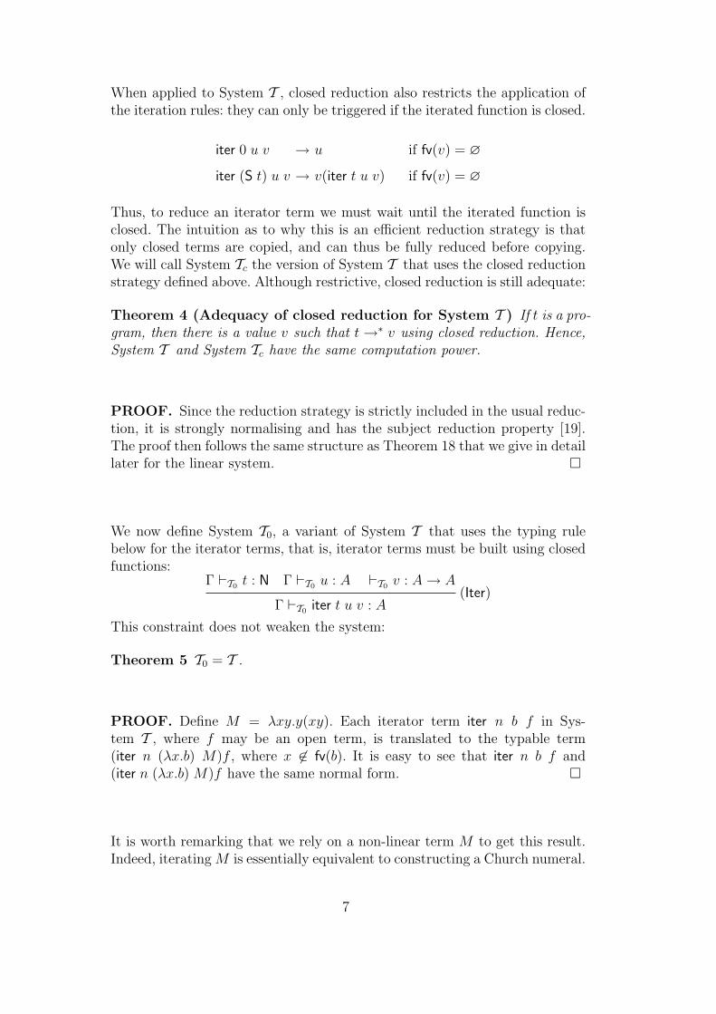
When applied to System T , closed reduction also restricts the application ofthe iteration rules: they can only be triggered if the iterated function is closed.

iter 0 u v → u if fv(v) = ∅

iter (S t) u v → v(iter t u v) if fv(v) = ∅

Thus, to reduce an iterator term we must wait until the iterated function isclosed. The intuition as to why this is an efficient reduction strategy is thatonly closed terms are copied, and can thus be fully reduced before copying.We will call System Tc the version of System T that uses the closed reductionstrategy defined above. Although restrictive, closed reduction is still adequate:

Theorem 4 (Adequacy of closed reduction for System T ) If t is a pro-gram, then there is a value v such that t→∗ v using closed reduction. Hence,System T and System Tc have the same computation power.

PROOF. Since the reduction strategy is strictly included in the usual reduc-tion, it is strongly normalising and has the subject reduction property [19].The proof then follows the same structure as Theorem 18 that we give in detaillater for the linear system.

We now define System T0, a variant of System T that uses the typing rulebelow for the iterator terms, that is, iterator terms must be built using closedfunctions:

Γ `T0 t : N Γ `T0 u : A `T0 v : A→ A(Iter)

Γ `T0 iter t u v : A

This constraint does not weaken the system:

Theorem 5 T0 = T .

PROOF. Define M = λxy.y(xy). Each iterator term iter n b f in Sys-tem T , where f may be an open term, is translated to the typable term(iter n (λx.b) M)f , where x 6∈ fv(b). It is easy to see that iter n b f and(iter n (λx.b) M)f have the same normal form.

It is worth remarking that we rely on a non-linear term M to get this result.Indeed, iterating M is essentially equivalent to constructing a Church numeral.

7

4 System L: a linear System T

We define System L, a linear version of System T , by extending the linearλ-calculus [1] with numbers, pairs, and an iterator with a closed reductionstrategy [13,18].

The set Λ of linear λ-terms t, u, . . . is inductively defined by: x ∈ Λ, λx.t ∈ Λif x ∈ fv(t), and tu ∈ Λ if fv(t)∩ fv(u) = ∅. Note that x is used at least once inthe body of the abstraction, and the condition on the application ensures thatall variables are used at most once. Thus these conditions ensure syntacticlinearity (variables occur exactly once).

In System L we will also have numbers generated by 0 and S, with an iterator:

iter t u v if fv(t) ∩ fv(u) = fv(u) ∩ fv(v) = fv(v) ∩ fv(t) = ∅

and pairs:

〈t, u〉 if fv(t) ∩ fv(u) = ∅

let 〈x, y〉 = t in u if x, y ∈ fv(u) and fv(t) ∩ (fv(u)− x, y) = ∅

Note that when projecting from a pair, we use both projections. A simpleexample of such a term is the function that swaps the components of a pair:

λx.let 〈y, z〉 = x in 〈z, y〉

Tuples of any size can be built from pairs. As an example, 〈x1, x2, x3〉 =〈x1, 〈x2, x3〉〉 and let 〈x1, x2, x3〉 = u in t represents the term

let 〈x1, y〉 = u in let 〈x2, x3〉 = y in t

Table 1 summarises the syntax of System L. The set of terms given by Table 1is called ΛL. Note that λ and let are binders; we work with terms moduloα-conversion as usual.

Definition 6 (Closed reduction) The reduction rules for System L are givenin Table 2. Substitution is a meta-operation defined as usual, and reductionscan take place in any context. We use the same symbol to denote the reductionrelation in System L and in System T since the intended relation will alwaysbe clear from the context.

Normal forms are not the same as in the λ-calculus: for example, λx.(λy.y)xis a normal form. Note that all the substitutions created during reduction(rules Beta and Let) are closed, and the Iter rules are only triggered when thefunction v is closed.

8

Terms Variable Constraint Free Variables (fv)

0 − ∅

S t − fv(t)

iter t u v fv(t) ∩ fv(u) = fv(u) ∩ fv(v) = ∅ fv(t) ∪ fv(u) ∪ fv(v)

fv(t) ∩ fv(v) = ∅

x − x

tu fv(t) ∩ fv(u) = ∅ fv(t) ∪ fv(u)

λx.t x ∈ fv(t) fv(t) r x

〈t, u〉 fv(t) ∩ fv(u) = ∅ fv(t) ∪ fv(u)

let 〈x, y〉 = t in u fv(t) ∩ (fv(u)− x, y) = ∅, x, y ∈ fv(u) fv(t) ∪ (fv(u) r x, y)

Table 1Terms in System L

Name Reduction Condition

Beta (λx.t)v −→ t[v/x] fv(v) = ∅

Let let 〈x, y〉 = 〈t, u〉 in v −→ (v[t/x])[u/y] fv(t) = fv(u) = ∅

Iter iter (S t) u v −→ v(iter t u v) fv(v) = ∅

Iter iter 0 u v −→ u fv(v) = ∅

Table 2Closed reduction

Lemma 7 (Correctness of substitution) Let t and u be System L terms.If z ∈ fv(t) and fv(u) = ∅, then t[u/z] is also a System L term. More generally,if fv(t) ∩ fv(u) = ∅ then t[u/z] satisfies the variable constraints.

PROOF. Straightforward induction on the structure of t.

Lemma 8 (Correctness of reduction) Let t be a System L term such thatt −→ u, then fv(t) = fv(u) and u is also a System L term.

PROOF. By simultaneous induction, showing that all the rewrite rules pre-serve the variable constraints given in Table 1.

Note that reduction preserves the free variables of the term, but the free vari-ables of a subterm may change. In particular, a subterm of the form iter n u v

9

may become closed after a reduction in a superterm, triggering in this way areduction with an Iter rule.

Although linear, System L is not strongly normalising. For instance, the termΩ = ∆∆ where

∆ = λx.iter S20 (λxy.xy) (λy.yx)

is non-terminating: Ω −→∗ Ω. In the remainder of this section we define alinear type system for System L and show that typable terms are stronglynormalisable.

4.1 Types for System L

The set of linear types is generated by the grammar:

A,B ::= N | A−B | A⊗B

Axiom(Axiom)

x : A `L x : A

Logical Rules

Γ, x : A `L t : B(−Intro)

Γ `L λx.t : A−B

Γ `L t : A−B ∆ `L u : A(−Elim)

Γ,∆ `L tu : B

Γ `L t : A ∆ `L u : B(⊗Intro)

Γ,∆ `L 〈t, u〉 : A⊗B

Γ `L t : A⊗B x : A, y : B,∆ `L u : C(⊗Elim)

Γ,∆ `L let 〈x, y〉 = t in u : C

Numbers(Zero)

`L 0 : N

Γ `L n : N(Succ)

Γ `L S n : N

Γ `L t : N Θ `L u : A ∆ `L v : A−A(Iter)

Γ,Θ,∆ `L iter t u v : A

Fig. 3. Type System for System L

We associate types to terms in System L using the typing rules given inFigure 3. We use a Curry-style type system; the typing rules specify how toassign types to untyped terms (there are no type decorations). Again, typingcontexts are sets of type assumptions of the form x: A, and dom(Γ) denotesthe set of variables such that xi : Ai ∈ Γ. Note that the axiom has exactly onetype assumption in the context, and we do not have weakening and contractionrules — we are in a linear system. For the same reason, the logical rules splitthe context between the premises. The rules for numbers are standard. In thecase of a term of the form iter t u v, we check that t is a term of type N andthat v and u are compatible.

10

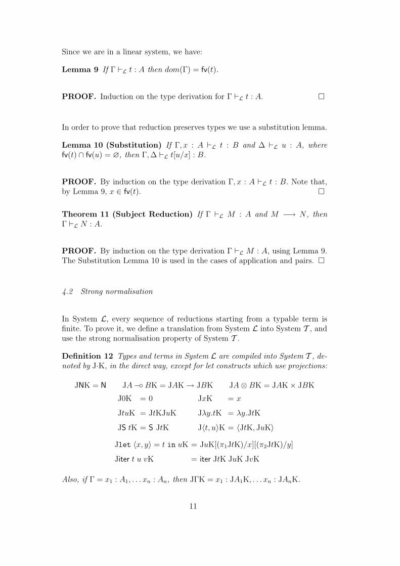
Since we are in a linear system, we have:

Lemma 9 If Γ `L t : A then dom(Γ) = fv(t).

PROOF. Induction on the type derivation for Γ `L t : A.

In order to prove that reduction preserves types we use a substitution lemma.

Lemma 10 (Substitution) If Γ, x : A `L t : B and ∆ `L u : A, wherefv(t) ∩ fv(u) = ∅, then Γ,∆ `L t[u/x] : B.

PROOF. By induction on the type derivation Γ, x : A `L t : B. Note that,by Lemma 9, x ∈ fv(t).

Theorem 11 (Subject Reduction) If Γ `L M : A and M −→ N , thenΓ `L N : A.

PROOF. By induction on the type derivation Γ `L M : A, using Lemma 9.The Substitution Lemma 10 is used in the cases of application and pairs.

4.2 Strong normalisation

In System L, every sequence of reductions starting from a typable term isfinite. To prove it, we define a translation from System L into System T , anduse the strong normalisation property of System T .

Definition 12 Types and terms in System L are compiled into System T , de-noted by J·K, in the direct way, except for let constructs which use projections:

JNK = N JA−BK = JAK→ JBK JA⊗BK = JAK× JBK

J0K = 0 JxK = x

JtuK = JtKJuK Jλy.tK = λy.JtK

JS tK = S JtK J〈t, u〉K = 〈JtK, JuK〉

Jlet 〈x, y〉 = t in uK = JuK[(π1JtK)/x][(π2JtK)/y]

Jiter t u vK = iter JtK JuK JvK

Also, if Γ = x1 : A1, . . . xn : An, then JΓK = x1 : JA1K, . . . xn : JAnK.

11

To simulate reductions we use the following properties, which are proved byroutine induction.

Lemma 13 (1) Let t, u be terms in System L such that fv(u) ∩ fv(t) = ∅and x ∈ fv(t). Then JtK[JuK/x] = Jt[u/x]K.

(2) If Γ `L t : T , then JΓK `T JtK : JTK.

Lemma 14 If t −→ t′, then JtK −→+ Jt′K.

PROOF. By induction on t. The only interesting cases are when t is anapplication or a let construct, and reduction takes place at the root position.In both cases the result follows from Lemma 13, part 1, because substitutionsare closed. We show the diagram for the case of a let construct.

let 〈x, y〉 = 〈a, b〉 in u - u[a/x][b/y]

JuK[π1J〈a, b〉K/x][π2J〈a, b〉K/y]

J·K

? ∗- JuK[JaK/x][JbK/y]

J·K(Lemma 13, 1)

?

Corollary 15 If JtK is strongly normalisable, so is t.

Theorem 16 (Strong normalisation) If Γ `L t : T , then t is strongly nor-malisable.

PROOF. Consequence of Lemma 13, SN of System T and Corollary 15.

4.3 Confluence and adequacy

System L is confluent, which implies that normal forms are unique. For typableterms, confluence is a direct consequence of strong normalisation and the factthat the rules are non-overlapping (using Newman’s Lemma [31]). In fact, allSystem L terms are confluent even if they are non-terminating: that can beproved using the Tait-Martin-Lof method. We refer to [2] for a detailed proof.

Theorem 17 (Confluence) −→ is Church-Rosser.

12

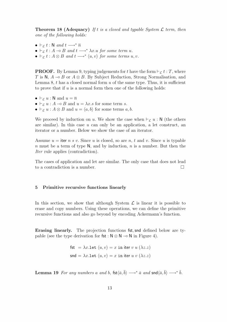
Theorem 18 (Adequacy) If t is a closed and typable System L term, thenone of the following holds:

• `L t : N and t −→∗ n• `L t : A−B and t −→∗ λx.u for some term u.• `L t : A⊗B and t −→∗ 〈u, v〉 for some terms u, v.

PROOF. By Lemma 9, typing judgements for t have the form `L t : T , whereT is N, A − B or A ⊗ B. By Subject Reduction, Strong Normalisation, andLemma 8, t has a closed normal form u of the same type. Thus, it is sufficientto prove that if u is a normal form then one of the following holds:

• `L u : N and u = n• `L u : A−B and u = λx.s for some term s.• `L u : A⊗B and u = 〈a, b〉 for some terms a, b.

We proceed by induction on u. We show the case when `L u : N (the othersare similar). In this case u can only be an application, a let construct, aniterator or a number. Below we show the case of an iterator.

Assume u = iter n s v. Since u is closed, so are n, t and v. Since u is typablen must be a term of type N, and by induction, n is a number. But then theIter rule applies (contradiction).

The cases of application and let are similar. The only case that does not leadto a contradiction is a number.

5 Primitive recursive functions linearly

In this section, we show that although System L is linear it is possible toerase and copy numbers. Using these operations, we can define the primitiverecursive functions and also go beyond by encoding Ackermann’s function.

Erasing linearly. The projection functions fst, snd defined below are ty-pable (see the type derivation for fst : N⊗ N− N in Figure 4).

fst = λx.let 〈u, v〉 = x in iter v u (λz.z)

snd = λx.let 〈u, v〉 = x in iter u v (λz.z)

Lemma 19 For any numbers a and b, fst〈a, b〉 −→∗ a and snd〈a, b〉 −→∗ b.

13

x : N⊗ N `L x : N⊗ N

v : N `L v : N u : N `L u : N

z : N `L z : N

`L λz.z : N− N

u : N, v : N `L iter v u λz.z : N

x : N⊗ N `L let 〈u, v〉 = x in iter v u (λz.z) : N

`L λx.let 〈u, v〉 = x in iter v u (λz.z) : (N⊗ N)− N

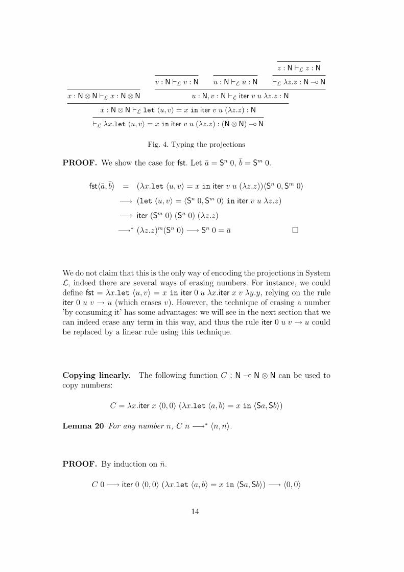
Fig. 4. Typing the projections

PROOF. We show the case for fst. Let a = Sn 0, b = Sm 0.

fst〈a, b〉 = (λx.let 〈u, v〉 = x in iter v u (λz.z))〈Sn 0, Sm 0〉

−→ (let 〈u, v〉 = 〈Sn 0, Sm 0〉 in iter v u λz.z)

−→ iter (Sm 0) (Sn 0) (λz.z)

−→∗ (λz.z)m(Sn 0) −→ Sn 0 = a

We do not claim that this is the only way of encoding the projections in SystemL, indeed there are several ways of erasing numbers. For instance, we coulddefine fst = λx.let 〈u, v〉 = x in iter 0 u λx.iter x v λy.y, relying on the ruleiter 0 u v → u (which erases v). However, the technique of erasing a number’by consuming it’ has some advantages: we will see in the next section that wecan indeed erase any term in this way, and thus the rule iter 0 u v → u couldbe replaced by a linear rule using this technique.

Copying linearly. The following function C : N − N ⊗ N can be used tocopy numbers:

C = λx.iter x 〈0, 0〉 (λx.let 〈a, b〉 = x in 〈Sa, Sb〉)

Lemma 20 For any number n, C n −→∗ 〈n, n〉.

PROOF. By induction on n.

C 0 −→ iter 0 〈0, 0〉 (λx.let 〈a, b〉 = x in 〈Sa, Sb〉) −→ 〈0, 0〉

14

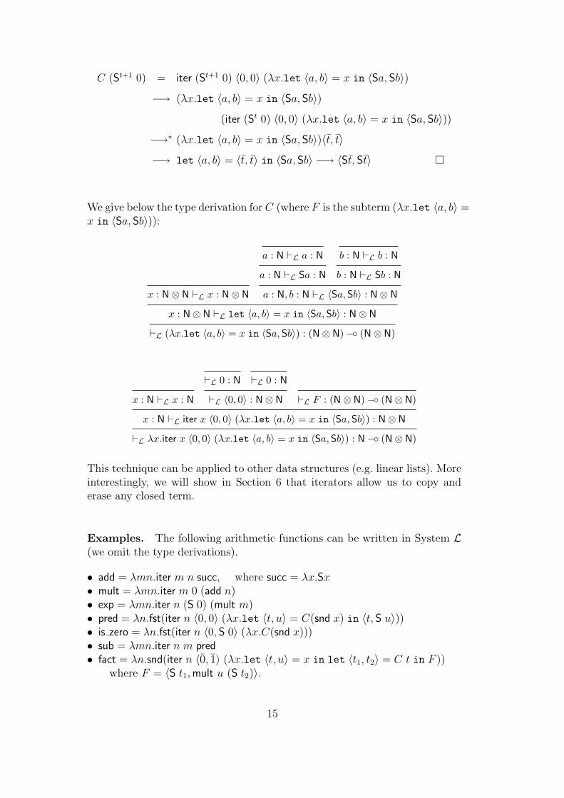
C (St+1 0) = iter (St+1 0) 〈0, 0〉 (λx.let 〈a, b〉 = x in 〈Sa, Sb〉)

−→ (λx.let 〈a, b〉 = x in 〈Sa, Sb〉)

(iter (St 0) 〈0, 0〉 (λx.let 〈a, b〉 = x in 〈Sa, Sb〉))

−→∗ (λx.let 〈a, b〉 = x in 〈Sa, Sb〉)〈t, t〉

−→ let 〈a, b〉 = 〈t, t〉 in 〈Sa, Sb〉 −→ 〈St, St〉

We give below the type derivation for C (where F is the subterm (λx.let 〈a, b〉 =x in 〈Sa, Sb〉)):

x : N⊗ N `L x : N⊗ N

a : N `L a : N

a : N `L Sa : N

b : N `L b : N

b : N `L Sb : N

a : N, b : N `L 〈Sa,Sb〉 : N⊗ N

x : N⊗ N `L let 〈a, b〉 = x in 〈Sa,Sb〉 : N⊗ N

`L (λx.let 〈a, b〉 = x in 〈Sa,Sb〉) : (N⊗ N)− (N⊗ N)

x : N `L x : N

`L 0 : N `L 0 : N

`L 〈0, 0〉 : N⊗ N `L F : (N⊗ N)− (N⊗ N)

x : N `L iter x 〈0, 0〉 (λx.let 〈a, b〉 = x in 〈Sa,Sb〉) : N⊗ N

`L λx.iter x 〈0, 0〉 (λx.let 〈a, b〉 = x in 〈Sa,Sb〉) : N− (N⊗ N)

This technique can be applied to other data structures (e.g. linear lists). Moreinterestingly, we will show in Section 6 that iterators allow us to copy anderase any closed term.

Examples. The following arithmetic functions can be written in System L(we omit the type derivations).

• add = λmn.iter m n succ, where succ = λx.Sx• mult = λmn.iter m 0 (add n)• exp = λmn.iter n (S 0) (mult m)• pred = λn.fst(iter n 〈0, 0〉 (λx.let 〈t, u〉 = C(snd x) in 〈t, S u〉))• is zero = λn.fst(iter n 〈0, S 0〉 (λx.C(snd x)))• sub = λmn.iter n m pred• fact = λn.snd(iter n 〈0, 1〉 (λx.let 〈t, u〉 = x in let 〈t1, t2〉 = C t in F ))

where F = 〈S t1,mult u (S t2)〉.

15

Primitive recursive functions. A function f : Nn → N is primitive recur-sive if it can be defined using the natural numbers, projections

πni (x1, . . . , xn) = xi, 1 ≤ i ≤ n

(we omit the superindex when there is no ambiguity), composition of func-tions, and the primitive recursive scheme, which allows us to define a recursivefunction h using two auxiliary primitive recursive functions f and g:

h(~x, 0) = f(~x)

h(~x, S n) = g(~x, h(~x, n), n)

The notation ~x is used as abbreviation for a sequence x1, . . . , xm. Note thatin the last equation, the numbers ~x and n are copied.

System L can express the whole class of primitive recursive functions. We havealready shown we can project, and of course we have composition. We nowshow how to encode a function h defined by primitive recursion from f and g.For simplicity we assume h is a binary function (h : N× N→ N).

First, assume h is defined by the following, simpler scheme (it uses n only oncein the second equation):

h(x, 0) = f(x)

h(x, n+ 1) = g(x, h(x, n))

Assume that there are closed terms in System L representing the functionsf and g; we will denote them by f and g since there is no ambiguity. Usingf : N− N and g : N− N− N, the function h can be defined by the typableterm (iter n f g′)x : N, where g′ is the term:

λy.λz.let 〈z1, z2〉 = C z in gz1(yz2) : (N− N)− (N− N)

Indeed, we can show by induction that (iter n f g′)x, where x and n arenumbers, reduces to the number h(x, n), using Lemma 20 to copy numbers.

Now to encode the standard primitive recursive scheme, which has an extra nin the last equation, all we need to do is copy n. We use the notation introducedabove (f, g are auxiliary functions, but g has now the type N−N−N−N):

h = λxn.let 〈n1, n2〉 = C n in s (pred n1) x

16

where pred is the predecessor function defined above and

s = iter n2 (λx1.(iter x1 I I)f) s′

s′ = λyx2z.

let 〈z1, z2〉 = C z in (let 〈w1, w2〉 = C x2 in g z1 (y (pred w1) z2) w2)

Beyond primitive recursion. Ackermann’s function is a standard exampleof a non primitive recursive function:

ack(0, n) = S n

ack(S n, 0) = ack(n, S 0)

ack(S n, S m) = ack(n, ack(S n,m))

In a higher-order functional language, there is an alternative definition. Letsucc = λx.S x : N− N, then ack(m,n) = a m n, where a is defined by:

a 0 = succ A g 0 = g(S 0)

a (S n) = A (a n) A g (S n) = g(A g n)

We can define a and A in System L as follows:

a = λn.iter n succ A : N− (N− N)

A = λgn.iter (S n) (S 0) g : (N− N)− N− N

We show by induction that this encoding is correct:

• a 0 −→ iter 0 succ A −→ succA g 0 −→∗ iter (S 0) (S 0) g −→∗ g(S 0)• a (S n) −→ iter (Sn 0) succ A −→ A(iter n succ A) −→∗ A(a n)A g (S n) −→∗ iter (S(S n)) (S 0) g −→ g(iter (S n) (S 0) g) −→∗ g(A g n).

Then Ackermann’s function can be defined in System L by the typable term:

ack = λmn.(iter m succ (λgu.iter (S u) (S 0) g)) n : N− N− N

Note that iter (S u) (S 0) g cannot be typed in the linear system defined in [11],because g is a free variable. We allow building the term with the free variableg, but we do not allow reduction until it is closed.

17

6 The power of System L

In this section, we show how to compile System T programs into System L;i.e., we show that System L has all the computation power of System T .

Explicit erasing. In the linear λ-calculus, we are not able to erase argu-ments. However, terms are consumed by reduction. The idea of erasing byconsuming is not new, it is related to solvability (see [9] for instance). Ourgoal in this section is to give an analogous result that allows us to obtain ageneral form of erasing.

Definition 21 (Erasing) We define the following mutually recursive oper-ations E and M, which, respectively, erase and create a System L term. IfΓ `L t : T , then E(t, T ) is defined as follows (where I = λx.x):

E(t,N) = iter t I I M(N) = 0

E(t, A−B) = E(tM(A), B) M(A−B) = λx.E(x,A)M(B)

E(t, A⊗B) = let 〈x, y〉 = t in E(x,A)E(y,B) M(A⊗B) = 〈M(A),M(B)〉

Lemma 22 If Γ `L t : T then:

(1) fv(E(t, T )) = fv(t) and Γ `L E(t, T ) : A− A, for any A.(2) M(T ) is a closed System L term such that `LM(T ) : T .

PROOF. Simultaneous induction on T .T = N:

• fv(E(t,N)) = fv(iter t I I) = fv(t), and Γ `L iter t I I : A− A, for any A.• fv(M(N)) = fv(0) = ∅, and `L 0 : N.

T = A⊗B:

• fv(E(t, A⊗B)) = fv(let 〈x, y〉 = t in E(x,A)E(y,B)) = fv(t). By induction:x : A `L E(x,A) : (C − C)− (C − C), y : B `L E(y,B) : C − C, then

x : A, y : B `L E(x,A)E(y,B) : C − C. Then Γ `L E(t, A ⊗ B) : C − C,for any C.• fv(M(A⊗B)) = fv(〈M(A),M(B)〉) = ∅ by IH(2), and `L 〈M(A),M(B)〉 :A⊗B by IH(2).

T = A−B:

18

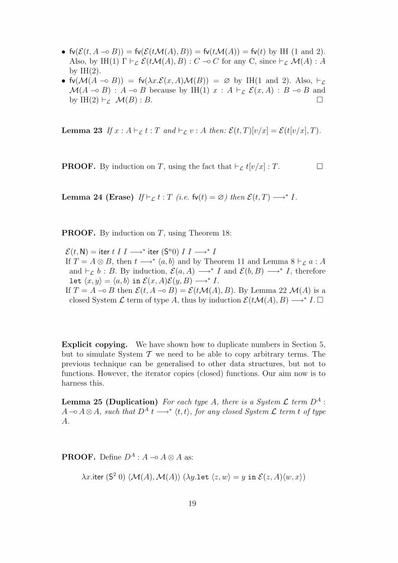
• fv(E(t, A − B)) = fv(E(tM(A), B)) = fv(tM(A)) = fv(t) by IH (1 and 2).Also, by IH(1) Γ `L E(tM(A), B) : C − C for any C, since `L M(A) : Aby IH(2).• fv(M(A − B)) = fv(λx.E(x,A)M(B)) = ∅ by IH(1 and 2). Also, `LM(A − B) : A − B because by IH(1) x : A `L E(x,A) : B − B andby IH(2) `L M(B) : B.

Lemma 23 If x : A `L t : T and `L v : A then: E(t, T )[v/x] = E(t[v/x], T ).

PROOF. By induction on T , using the fact that `L t[v/x] : T .

Lemma 24 (Erase) If `L t : T (i.e. fv(t) = ∅) then E(t, T ) −→∗ I.

PROOF. By induction on T , using Theorem 18:

E(t,N) = iter t I I −→∗ iter (Sn0) I I −→∗ IIf T = A⊗ B, then t −→∗ 〈a, b〉 and by Theorem 11 and Lemma 8 `L a : Aand `L b : B. By induction, E(a,A) −→∗ I and E(b, B) −→∗ I, thereforelet 〈x, y〉 = 〈a, b〉 in E(x,A)E(y,B) −→∗ I.

If T = A− B then E(t, A− B) = E(tM(A), B). By Lemma 22 M(A) is aclosed System L term of type A, thus by induction E(tM(A), B) −→∗ I.

Explicit copying. We have shown how to duplicate numbers in Section 5,but to simulate System T we need to be able to copy arbitrary terms. Theprevious technique can be generalised to other data structures, but not tofunctions. However, the iterator copies (closed) functions. Our aim now is toharness this.

Lemma 25 (Duplication) For each type A, there is a System L term DA :A−A⊗A, such that DA t −→∗ 〈t, t〉, for any closed System L term t of typeA.

PROOF. Define DA : A− A⊗ A as:

λx.iter (S2 0) 〈M(A),M(A)〉 (λy.let 〈z, w〉 = y in E(z, A)〈w, x〉)

19

Now it is straightforward to show that:

DA t −→ iter (S2 0) 〈M(A),M(A)〉 (λy.let 〈z, w〉 = y in E(z, A)〈w, t〉)

−→∗ (λy.let 〈z, w〉 = y in E(z, A)〈w, t〉)2〈M(A),M(A)〉

−→∗ (λy.let 〈z, w〉 = y in E(z, A)〈w, t〉)(E(M(A), A)〈M(A), t〉)

−→∗ (λy.let 〈z, w〉 = y in E(z, A)〈w, t〉)〈M(A), t〉

−→∗ E(M(A), A)〈t, t〉 −→∗ 〈t, t〉

A function of type A ⊗ A − A ⊗ A is iterated, and this idea can also scaleup, e.g.: DA

3 : A− A⊗ A⊗ A. The base will be 〈M(A),M(A),M(A)〉, anditerate a function A3 − A3. This result also applies to numbers, so we havetwo different ways of copying numbers in System L.

Definition 26 (Duplicator) For n > 1, we define a generalised duplicatorDA

n : A− A⊗ · · · ⊗ A︸ ︷︷ ︸n

, as:

λx.iter (Sn 0) 〈M(A), . . . ,M(A)〉 (λy.let 〈x1, . . . , xn〉 = y in E(x1, A)〈x2, . . . , xn, x〉)

6.1 Compilation

We now put the previous ideas together to give a formal compilation of SystemT into System L.

Definition 27 System T types are translated into System L types using 〈〈·〉〉defined by:

〈〈N〉〉 = N 〈〈A→ B〉〉 = 〈〈A〉〉 − 〈〈B〉〉 〈〈A×B〉〉 = 〈〈A〉〉 ⊗ 〈〈B〉〉

If Γ = x1 : T1, . . . , xn : Tn then 〈〈Γ〉〉 = x1 : 〈〈T1〉〉, . . . , xn : 〈〈Tn〉〉.

We will now translate typable terms from System T into typable System Lterms. Recall that by Lemma 1, part 2, if t is typable in System T then thereexists a type derivation Γ `T t : T where dom(Γ) = fv(t).

In the remainder of this paper, for convenience, we make the following abbre-viations:

Cx1,...,xn

x:A t = let 〈x1, . . ., xn〉 = DAn x in t

Axyt = ([x]t)[y/x], where [x]t is defined below.

20

Definition 28 (Compilation) Let t be a System T term such that fv(t) =x1, . . . , xn, n ≥ 0, and x1:A1, . . . , xn:An `T t : T . Its compilation into Sys-tem L is defined as: [xA1

1 ] . . . [xAnn ]〈〈t〉〉, 1 where we assume without loss of gen-

erality that the variables are processed in lexicographic order, and 〈〈·〉〉, [·]· aredefined below by induction. Note that [x]t is only defined when x ∈ fv(t).

〈〈x〉〉 = x

〈〈su〉〉 = 〈〈s〉〉〈〈u〉〉

〈〈λx.u〉〉 = λx.[x]〈〈u〉〉, if x ∈ fv(u)

= λx.E(x, 〈〈A〉〉)〈〈u〉〉, otherwise,

where x1:A1, . . . , xn:An `T t : A→ B = T by Lemma 1

〈〈0〉〉 = 0

〈〈S u〉〉 = S〈〈u〉〉

〈〈iter n u v〉〉 = iter 〈〈n〉〉 〈〈u〉〉 〈〈v〉〉

〈〈〈s, u〉〉〉 = 〈〈〈s〉〉, 〈〈u〉〉〉

〈〈π1s〉〉 = let 〈x, y〉 = 〈〈s〉〉 in E(y, 〈〈B〉〉)x,

where x1:A1, . . . , xn:An `T t : A×B = T by Lemma 1

〈〈π2s〉〉 = let 〈x, y〉 = 〈〈s〉〉 in E(x, 〈〈A〉〉)y,

where x1:A1, . . . , xn:An `T t : A×B = T by Lemma 1

[x](S u) = S([x]u)

[x]x = x

[x](λy.u) = λy.[x]u

[xA](su) =

Cx1,x2

x:A (Axx1s)(Ax

x2u) x ∈ fv(s), x ∈ fv(u)

([x]s)u x ∈ fv(s), x 6∈ fv(u)

s([x]u) x ∈ fv(u), x 6∈ fv(s)

[xA]〈s, u〉 =

Cx1,x2

x:A 〈Axx1s, Ax

x2u〉, x ∈ fv(s), x ∈ fv(u)

〈[x]s, u〉, x ∈ fv(s), x 6∈ fv(u)

〈s, [x]u〉, x ∈ fv(u), x 6∈ fv(s)

1 We will omit the types of the variables x1, . . . , xn in the compilation when theyare not necessary.

21

[xA](let 〈y, z〉 = s in u) =

let 〈y, z〉 = [x]s in u x ∈ fv(s), x 6∈ fv(u)

let 〈y, z〉 = s in [x]u x 6∈ fv(s), x ∈ fv(u)

Cx1,x2

x:A (let 〈y, z〉 = Axx1s in Ax

x2u) x ∈ fv(s), x ∈ fv(u)

[xA](iter n u v) =

iter [x]n u v x ∈ fv(n), x 6∈ fv(uv)

iter n [x]u v x 6∈ fv(nv), x ∈ fv(u)

iter n u [x]v x 6∈ fv(nu), x ∈ fv(v)

Cx1,x2

x:A iter (Axx1n) (Ax

x2u) v x ∈ fv(n) ∩ fv(u), x 6∈ fv(v)

Cx1,x3

x:A iter (Axx1n) u (Ax

x3v) x ∈ fv(n) ∩ fv(v), x 6∈ fv(u)

Cx2,x3

x:A iter n (Axx2u) (Ax

x3v) x 6∈ fv(n), x ∈ fv(u) ∩ fv(v)

Cx1,x2,x3

x:A iter (Axx1n) (Ax

x2u) (Ax

x3v) x ∈ fv(n) ∩ fv(u) ∩ fv(v)

where the variables x1, x2 and x3 above are assumed fresh.

Examples. To illustrate the encoding, we show the compilation of the com-binators:

• 〈〈λx.x〉〉 = λx.x.• 〈〈λxyz.xz(yz)〉〉 = λxyz.let 〈z1, z2〉 = DA

2 z in xz1(yz2),with `T λxyz.xz(yz) : (A→ B → C)→ (A→ B)→ A→ C.

• 〈〈λxy.x〉〉 = λxy.E(y,B)x, with `T λxy.x : A→ B → A.

A more interesting example is the following definition of the predecessor func-tion. Define first the term: P = λn.iter n 〈I, 0〉 λw.let 〈u, v〉 = w in 〈succ, uv〉,where succ = λx.S x : N− N. Since the function in the iterator is closed, wehave:

P 0 −→ 〈I, 0〉

P (S n) −→∗ 〈succ, n〉To define the predecessor function we just need to add a projection. We usethe encoding of π2t, 〈〈π2t〉〉, given in Definition 28:

Pred = λn.let P n = 〈x, y〉 in (iter (x 0) I I)y.

The rest of this section is devoted to the proof of correctness of the compilationfunction; for more details and examples see [2]. First we show that the resultof the compilation of a System T term satisfies the linearity constraints ofSystem L.

Definition 29 Consider a finite set of variables X. We say that a term t isin Λ+X

L , if t is a term built using the syntax of ΛL, for which the linearityconditions hold for all its bound variables and also for the free variables in X.Note that, if X = fv(t), then t is a term in ΛL (i.e., the variable constraintshold for all its variables).

22

Example 30 Let X1 = x, y, z and X2 = x, y. The term S3(0) is in bothΛ+X1L and Λ+X2

L . The term 〈xz, yz〉 is in Λ+X2L , but not in Λ+X1

L .

Proposition 31 If t is a term in Λ+XL , and x /∈ fv(t), then t is in Λ

+(X∪x)L .

Lemma 32 If t is a term in Λ+XL , and x is a free variable in t, then:

(1) fv([x]t) = fv(t)

(2) [x]t is a term in Λ+(X∪x)L

PROOF. First note that the duplicating term D is a closed term, in Λ+XL ,

for any set of variables X. The lemma is proved by simultaneous inductionon t. We show the case of an application term (pairs and iterators are treatedsimilarly, the other cases follow directly by induction):

• t ≡ uv, and x ∈ fv(u), x /∈ fv(v) (the case x /∈ fv(u), x ∈ fv(v) is similar).

(1) fv([x]uv) = fv(([x]u)v) = fv([x]u) ∪ fv(v)(I.H.)= fv(u) ∪ fv(v) = fv(uv)

(2) [x](uv) = ([x]u)v. By induction hypothesis [x]u is in Λ+(X∪x)L and v is

in Λ+(X∪x)L by Proposition 31. By hypothesis fv(u) ∩ fv(v) ∩X = ∅. By

induction hypothesis (1) fv([x]u) = fv(v), thus fv([x]u)∩fv(v)∩(X∪x) =

∅ (because x /∈ fv(v)). Therefore ([x]u)v is in Λ+(X∪x)L .

• t ≡ uv, and x ∈ fv(u), x ∈ fv(v). Then(1) In the following, note that if x ∈ t, then fv(t[y/x]) = (fv(t) \ x) ∪ y.

fv([x]uv) = fv(let 〈x1, x2〉 = Dx in (([x]u)[x1/x])(([x]v)[x2/x]))

= fv(Dx) ∪ (fv((([x]u)[x1/x])(([x]v)[x2/x]))) \ x1, x2

= x ∪ ((fv([x]u) \ x) ∪ x1 ∪ ((fv([x]v) \ x) ∪ x2) \ x1, x2)(I.H.)= x ∪ ((fv(u) \ x) ∪ (fv(v) \ x))

= fv(uv)

(2) [x](uv) = let 〈x1, x2〉 = Dx in (([x]u)[x1/x])(([x]v)[x2/x])By induction hypothesis (1):

fv([x]u) = fv(u) = Yu ∪ x

fv([x]v) = fv(v) = Yv ∪ x

By hypothesis, fv(u) ∩ fv(v) ∩X = ∅, thus Yu ∩ Yv ∩X = ∅. Note that

fv(([x]u)[x1/x]) = Yu ∪ x1

fv(([x]v)[x2/x]) = Yv ∪ x2

23

Therefore fv(Axx1u) ∩ fv(Ax

x2v) ∩ (X ∪ x) = ∅, then (Ax

x1u)(Ax

x2v) ∈

Λ+(X∪x)L . Also, fv(Dx) = x and Dx is a term in Λ

+(X∪x)L for any set of

variables X. Thus, fv(Dx)∩fv((Axx1u)(Ax

x2v))∩(X∪x) = ∅, and x1, x2 ∈

fv(Axx1u)(Ax

x2v), therefore let 〈x1, x2〉 = Dx in (([x]u)[x1/x])(([x]v)[x2/x]) ∈

Λ+(X∪x)L .

Lemma 33 Let t be a System T term, then fv(〈〈t〉〉) = fv(t).

PROOF. By a routine induction on t, using Lemma 32.

Lemma 34 Let t be a System T term, then 〈〈t〉〉 is a term in Λ+∅L .

PROOF. The only non trivial cases are abstractions and projections.

• t ≡ λx.u, and x ∈ fv(u). Then 〈〈t〉〉 = λx.[x]〈〈u〉〉. By induction hypothesis 〈〈u〉〉is a term in Λ+∅

L and by Lemma 32 x ∈ fv([x]〈〈u〉〉), therefore λx.[x]〈〈u〉〉 is inΛ+∅L .

• t ≡ λx.u, and x 6∈ fv(u). Then 〈〈t〉〉 = λx.(E(x, 〈〈A〉〉)〈〈u〉〉). By inductionhypothesis 〈〈u〉〉 is in Λ+∅

L , and since E(x, 〈〈A〉〉) is a System L term, thereforeis in Λ+∅

L . Since fv(E(x, 〈〈A〉〉)) ∩ fv(〈〈u〉〉) = ∅, then E(x, 〈〈A〉〉)〈〈u〉〉 is in Λ+∅L ,

and since x ∈ fv(E(x, 〈〈A〉〉)〈〈u〉〉), then λx.(E(x, 〈〈A〉〉)〈〈u〉〉) is in Λ+∅L .

• t ≡ π1(u). Then 〈〈t〉〉 = let 〈x, y〉 = 〈〈u〉〉 in E(y, 〈〈A2〉〉)x. By inductionhypothesis 〈〈u〉〉 is in Λ+∅

L . The terms E(y, 〈〈A2〉〉) and x are both in Λ+∅L , and

since fv(E(y, 〈〈A2〉〉)) ∩ fv(x) = ∅, then E(y, 〈〈A2〉〉)x is in Λ+∅L , and x, y ∈

fv(E(y, 〈〈A2〉〉)x), therefore let 〈x, y〉 = 〈〈u〉〉 in E(y, 〈〈A2〉〉)x is in Λ+∅L .

Lemma 35 If t is a System T term, then:

(1) fv([x1] · · · [xn]〈〈t〉〉) = fv(t).(2) If fv(t) = x1, . . . , xn, then [x1] · · · [xn]〈〈t〉〉 is in ΛL.

PROOF.

(1) By induction on the number of variables n using Lemmas 32 and 33.(2) By Lemma 34, 〈〈t〉〉 is a term in Λ+∅

L . By induction on the number of

variables n, using part 2 of Lemma 32, [x1] · · · [xn]〈〈t〉〉 is a term in Λ+fv(t)L ,

therefore a term in ΛL.

Lemma 35 states that the result of the compilation of a System T term is aSystem L term. We will now prove that the compilation of a typable term is

24

also typable (Theorem 38). For this, we will show that the terms obtained inthe intermediate steps of the compilation can be typed in a hybrid system,obtained from System L by allowing weakening and contraction only for vari-ables in a certain set X (i.e., we relax the linear constraints for the variables inX). Typing judgements in this system will be denoted Γ `L+X t : T . A typingcontext Γ is still a set of assumptions of the form x:A, where each variableoccurs at most once. The axiom for System L+X is:

Γ, x : A ` x : A where dom(Γ) ⊆ X

The typing rules are the same as in System L, except that in the rules thatsplit a typing context between the premisses in System L, now we can sharevariables in X. For instance, in the rule −Elim (see Figure 3) used to typeapplication terms uv, we may have fv(u) ∩ fv(v) ⊆ X and dom(Γ ∩∆) ⊆ X.

Note that if X = ∅ then L+X coincides with System L.

We will denote by Γ|X the restriction of Γ to the variables in X.

Lemma 36 If Γ `L+X t : A, where dom(Γ) = fv(t) and x ∈ X ⊆ fv(t), thenΓ `L+X′ [x]t : A, where X ′ = X \ x.

PROOF. By induction on t, using the fact that x : A `L+∅ Dx : A⊗ A. Weshow the cases for variable and application.

• t ≡ x. Then [x]x = x, and using the axiom we obtain both x : A `L+x x : Aand x : A `L+∅ x : A.• t ≡ uv, and x ∈ fv(u), x /∈ fv(v) (the case where x /∈ fv(u), x ∈ fv(v) is

similar). Then [x]uv = ([x]u)v and Γ `L+X uv : A. Let Γ1 = Γ|fv(u)and

Γ2 = Γ|fv(v). Then Γ1 `L+X u : B − A and Γ2 `L+X v : B, where Γ1 and

Γ2 can only share variables in X. By induction hypothesis Γ1 `L+X′ [x]u :B −A. Also, since x /∈ fv(v) and dom(Γ2) = fv(v), we have Γ2 `L+X′ v : B.Therefore Γ `L+X′ (x[u])v : A.• t ≡ uv, x ∈ fv(u), and x ∈ fv(v). Let Γ1 = Γ|fv(u)\x and Γ2 = Γ|fv(v)\x and

assume C is the type associated to x in Γ. Then Γ1, x : C `L+X u : B−A andΓ2, x : C `L+X v : B. By induction hypothesis Γ1, x : C `L+X′ [x]u : B−A,and Γ2, x : C `L+X′ [x]v : B. Thus Γ1, x1 : C `L+X′ ([x]u)[x1/x] : B − A,and Γ2, x2 : C `L+X′ ([x]v)[x2/x] : B. Therefore Γ1, x1 : C,Γ2, x2 : C `L+X′

(Axx1u)(Ax

x2v) : A. Also x : C `L+∅ Dx : C⊗C, therefore Γ1,Γ2, x : C `L+X′

let 〈x1, x2〉 = Dx in (Axx1u)(Ax

x2v) : A

Lemma 37 If Γ `T t : A, then 〈〈Γ|fv(t)〉〉 `L+fv(t) 〈〈t〉〉 : 〈〈A〉〉.

25

PROOF. By induction on the type derivation Γ `T t : A. We distinguishcases depending on the last typing rule applied. Below we show a few inter-esting cases.

• →Intro: Γ `T λx.u : A1 → A2 if Γ, x : A1 `T u : A2. By induction hypothe-sis, 〈〈(Γ, x : A1)|fv(u)

〉〉 `L+fv(u) 〈〈u〉〉 : 〈〈A2〉〉. There are two cases:

· x ∈ fv(u). Then 〈〈λx.u〉〉 = (λx.[x]〈〈u〉〉), and (Γ, x:A1)|fv(u)= Γ|fv(u)

, x:A1.

Thus 〈〈Γ|fv(u)〉〉, x:〈〈A1〉〉 `L+fv(u) 〈〈u〉〉 : 〈〈A2〉〉.

By Lemma 36, 〈〈Γ|fv(u)〉〉, x:〈〈A1〉〉 `L+fv(t) [x]〈〈u〉〉 : 〈〈A2〉〉.

Hence, 〈〈Γ|fv(t)〉〉 `L+fv(t) λx.[x]〈〈u〉〉 : 〈〈A1〉〉 − 〈〈A2〉〉.

· x /∈ fv(u), thus fv(t) = fv(u). Then 〈〈λx.u〉〉 = (λx.E(x, 〈〈A1〉〉)〈〈u〉〉), (Γ, x :A1)|fv(u)

= Γ|fv(t)and 〈〈Γ|fv(t)

〉〉 `L+fv(t) 〈〈u〉〉 : 〈〈A2〉〉. By Lemma 22, x:〈〈A1〉〉 `L∅

E(x, 〈〈A1〉〉) : 〈〈A2〉〉−〈〈A2〉〉, hence 〈〈Γ|fv(t)〉〉, x:〈〈A1〉〉 `L+fv(t) E(x, 〈〈A1〉〉)〈〈u〉〉 : 〈〈A2〉〉.

Thus 〈〈Γ|fv(t)〉〉 `L+fv(t) λx.E(x, 〈〈A1〉〉)〈〈u〉〉 : 〈〈A1〉〉 − 〈〈A2〉〉.

• ×Elim: Γ `T π1u : A1 if Γ `T u : A1 × A2. By induction hypothesis〈〈Γ|fv(u)

〉〉 `L+fv(u) 〈〈u〉〉 : 〈〈A1〉〉 ⊗ 〈〈A2〉〉. By Lemma 22 y : 〈〈A2〉〉 `L∅ E(y, 〈〈A2〉〉) :

〈〈A1〉〉 − 〈〈A1〉〉. Also x : 〈〈A1〉〉 `L∅ x : 〈〈A1〉〉, therefore y : 〈〈A2〉〉, x : 〈〈A1〉〉 `L∅

E(y, 〈〈A2〉〉)x : 〈〈A1〉〉.Thus 〈〈Γ|fv(t)

〉〉 `L+fv(t) let 〈x, y〉 = 〈〈u〉〉 in E(y, 〈〈A2〉〉)x : 〈〈A1〉〉.

Theorem 38 If Γ `T t : T and fv(t) = x1, . . . , xn then

〈〈Γ|fv(t)〉〉 `L [x1] . . . [xn]〈〈t〉〉 : 〈〈T 〉〉.

PROOF. By induction on the number of free variables of t, using Lemmas 36and 37.

We will now prove that we can simulate System T evaluations. First we needa substitution lemma.

Lemma 39 (1) If t is in Λ+XL , x, y ∈ fv(t), and fv(u) = ∅, then

([y]t)[u/x] = [y](t[u/x]).(2) If t is a System T term, x ∈ fv(t), and fv(u) = ∅, then〈〈t〉〉[〈〈u〉〉/x] = 〈〈t[u/x]〉〉

PROOF. By induction on t, see Definition 29 and Lemma 32.

Lemma 40 If t ∈ Λ+XL , x ∈ fv(t), and fv(u) = ∅ then ([x]t)[u/x] −→∗ t[u/x].

26

PROOF. By induction on t; below we show the case of application.

• t ≡ sv, x ∈ fv(s), x 6∈ fv(v) (the case x 6∈ fv(s), x ∈ fv(v) is similar).

([x]sv)[u/x] = (([x]s)v)[u/x]

= (([x]s)[u/x])v(I.H.)

−→∗ (s[u/x])v = (sv)[u/x]

• t ≡ sv, x ∈ fv(s), x ∈ fv(v).

([x]sv)[u/x] = let 〈x1, x2〉 = Dx in (([x]s)[x1/x])(([x]v)[x2/x])[u/x]

= let 〈x1, x2〉 = Du in (([x]s)[x1/x])(([x]v)[x2/x])

−→∗ let 〈x1, x2〉 = 〈u, u〉 in (([x]s)[x1/x])(([x]v)[x2/x])

−→ (([x]s)[u/x])(([x]v)[u/x])(I.H.)

−→∗ (s[u/x])(v[u/x]) = (sv)[u/x]

Theorem 41 (Simulation) Let t be a closed, typable System T term, then:

t ⇓ u⇒ 〈〈t〉〉 −→∗ 〈〈u〉〉.

PROOF. By induction on t ⇓ u (see Figure 2). We show two cases:

Application. By induction: 〈〈tu〉〉 = 〈〈t〉〉〈〈u〉〉 −→∗ 〈〈λx.t′〉〉〈〈u〉〉. There are now twocases:

• If x ∈ fv(t′) then using Lemma 40:

〈〈λx.t′〉〉〈〈u〉〉 = (λx.[x]〈〈t′〉〉)〈〈u〉〉 −→ ([x]〈〈t′〉〉)[〈〈u〉〉/x] −→∗ 〈〈t′[u/x]〉〉 −→∗ 〈〈v〉〉

• Otherwise, using Lemmas 23 and 24:

〈〈λx.t′〉〉〈〈u〉〉 = (λx.E(x,A)〈〈t′〉〉)〈〈u〉〉

−→∗ (E(〈〈u〉〉, 〈〈A〉〉)〈〈t′〉〉) −→ 〈〈t′〉〉 = 〈〈t′[u/x]〉〉 −→∗ 〈〈v〉〉

Projection. By induction and Lemmas 23 and 24:

〈〈π1t〉〉 = let 〈x, y〉 = 〈〈t〉〉 in E(y, 〈〈A〉〉)x

−→∗ let 〈x, y〉 = 〈〈〈u, v〉〉〉 in E(y, 〈〈A〉〉)x

= let 〈x, y〉 = 〈〈〈u〉〉, 〈〈v〉〉〉 in E(y, 〈〈A〉〉)x −→ E(〈〈v〉〉, 〈〈A〉〉)〈〈u〉〉 −→∗ 〈〈v〉〉

As a corollary we get that T = L.

27

7 Closed reduction, closed construction, and linearity

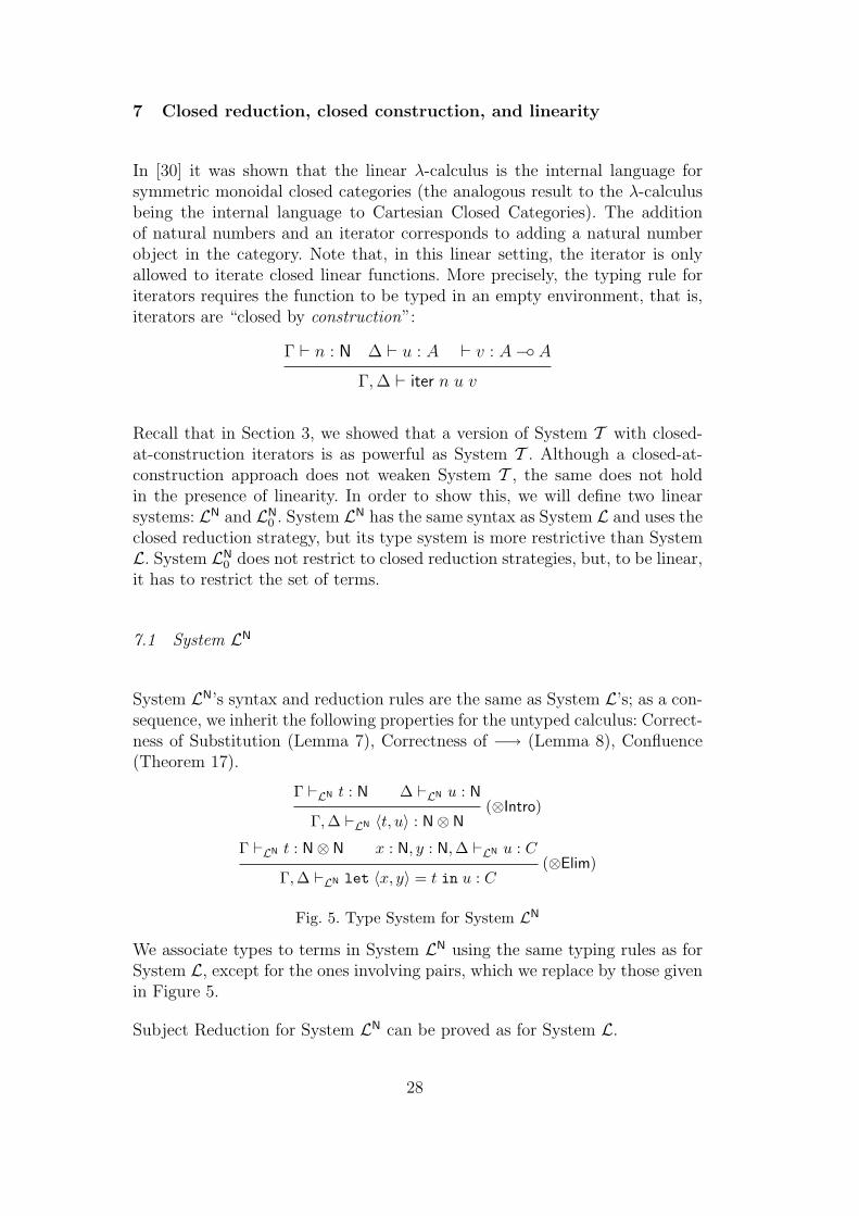
In [30] it was shown that the linear λ-calculus is the internal language forsymmetric monoidal closed categories (the analogous result to the λ-calculusbeing the internal language to Cartesian Closed Categories). The additionof natural numbers and an iterator corresponds to adding a natural numberobject in the category. Note that, in this linear setting, the iterator is onlyallowed to iterate closed linear functions. More precisely, the typing rule foriterators requires the function to be typed in an empty environment, that is,iterators are “closed by construction”:

Γ ` n : N ∆ ` u : A ` v : A− A

Γ,∆ ` iter n u v

Recall that in Section 3, we showed that a version of System T with closed-at-construction iterators is as powerful as System T . Although a closed-at-construction approach does not weaken System T , the same does not holdin the presence of linearity. In order to show this, we will define two linearsystems: LN and LN

0 . System LN has the same syntax as System L and uses theclosed reduction strategy, but its type system is more restrictive than SystemL. System LN

0 does not restrict to closed reduction strategies, but, to be linear,it has to restrict the set of terms.

7.1 System LN

System LN’s syntax and reduction rules are the same as System L’s; as a con-sequence, we inherit the following properties for the untyped calculus: Correct-ness of Substitution (Lemma 7), Correctness of −→ (Lemma 8), Confluence(Theorem 17).

Γ `LN t : N ∆ `LN u : N(⊗Intro)

Γ,∆ `LN 〈t, u〉 : N⊗ N

Γ `LN t : N⊗ N x : N, y : N,∆ `LN u : C(⊗Elim)

Γ,∆ `LN let 〈x, y〉 = t in u : C

Fig. 5. Type System for System LN

We associate types to terms in System LN using the same typing rules as forSystem L, except for the ones involving pairs, which we replace by those givenin Figure 5.

Subject Reduction for System LN can be proved as for System L.

28

Note that confluence of the untyped calculus, together with subject reduction,implies confluence of the typed calculus.

Since terms typable in System LN are also typable in System L, we inheritthe strong normalisation property.

7.2 System LN0

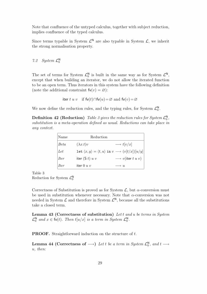
The set of terms for System LN0 is built in the same way as for System LN,

except that when building an iterator, we do not allow the iterated functionto be an open term. Thus iterators in this system have the following definition(note the additional constraint fv(v) = ∅):

iter t u v if fv(t)∩fv(u)=∅ and fv(v)=∅

We now define the reduction rules, and the typing rules, for System LN0 .

Definition 42 (Reduction) Table 3 gives the reduction rules for System LN0 ,

substitution is a meta-operation defined as usual. Reductions can take place inany context.

Name Reduction

Beta (λx.t)v −→ t[v/x]

Let let 〈x, y〉 = 〈t, u〉 in v −→ (v[t/x])[u/y]

Iter iter (S t) u v −→ v(iter t u v)

Iter iter 0 u v −→ u

Table 3Reduction for System LN

0

Correctness of Substitution is proved as for System L, but α-conversion mustbe used in substitution whenever necessary. Note that α-conversion was notneeded in System L and therefore in System LN, because all the substitutionstake a closed term.

Lemma 43 (Correctness of substitution) Let t and u be terms in SystemLN

0 and x ∈ fv(t). Then t[u/x] is a term in System LN0 .

PROOF. Straightforward induction on the structure of t.

Lemma 44 (Correctness of −→) Let t be a term in System LN0 , and t −→

u, then:

29

(1) fv(t) = fv(u);(2) u is a System LN

0 term.

PROOF. (Sketch) The only reduction rules that copy or erase terms, are therules for iterators, which either copy or erase the iterated function. However,because of the condition that the iterated function must be closed when con-structing the term iter t u v, then reducing an iterator will either copy or erasea closed term. Therefore the set of free variables is preserved and the termobtained is valid.

We associate types to terms in System LN0 using the same typing rules as

for System LN, except for the (Iter) rule, where the context for the iteratedfunction is always empty. Therefore, iterators is System LN

0 are typed in thefollowing way:

Γ `LN0t : N Θ `LN

0u : A `LN

0v : A→ A

(Iter)Γ,Θ `LN

0iter t u v : A

As before, Subject Reduction for System LN0 can be proved as for System L.

Note that any term typable in System LN0 is also typable in System LN, there-

fore in System L. Thus, System LN0 is strongly normalisable.

Confluence for typable terms in System LN0 is a direct consequence of strong

normalisation and the fact that the rules are non-overlapping (using New-man’s Lemma [31]). Moreover, we can apply directly Klop’s result [25] to theuntyped calculus because the system is orthogonal (that is, left-linear andnon-overlapping).

7.3 Primitive recursive functions and beyond

The encodings of the projections fst and snd, the copying function C, and theprimitive recursive scheme, given for System L in Section 5, satisfy the termconditions of System LN

0 , and therefore also those of System LN. The reduc-tions are valid in both systems, and the terms are typable in the more restrictedtype systems of System LN

0 and System LN. Note that, to encode primitive re-cursive functions, one only needs pairs of natural numbers. Also, the encodingsin Section 5 only iterate functions that are closed-by-construction, thereforetypable in System LN

0 .

On the other hand, the encoding of Ackermann’s function given for SystemL using functions a and A is still valid in System LN. However, note that

30

iter (S u) (S 0) g cannot be typed in System LN0 , because g is a free variable.

System LN allows building the term with the free variable g, but does notallow reduction until it is closed.

The fact that Ackermann’s function cannot be defined in System LN0 is ex-

pected, as it can be seen as a subsystem of Dal Lago’s linear languageH(∅) [11],albeit with a different syntax. Therefore System LN

0 is strictly less powerfulthan System LN because we cannot define Ackermann’s function in H(∅) (see[11] for a proof of this result).

7.4 Discussion

In Section 3, we showed that restricting the iterators using the closed-at-construction approach does not affect the computational power of System T .A linear system with the same restriction is, however, strictly less powerfulthan a system using a closed-reduction approach, as shown in Section 7. Aclosed-reduction approach interacts well with linearity: System L (a linearsystem with closed-reduction) proved to be as powerful as System T .

It remains to understand the role of product types in the linear systems, ormore precisely, the relationship between System L and System LN. If one re-stricts pairs to natural numbers, then one loses the ability to define duplicationof any term, as was done in Section 6. In [3], we presented a linear system, aspowerful as System T , where pairs were not crucial to define duplication, how-ever, iterators where typed using a kind of polymorphic types, which we callediterator types. This suggests that pairs also play a role and add computationalpower to System L.

8 Conclusions and future work

We have shown that in a linear λ-calculus with iterators (System L), the useof a ‘closed-at-reduction’ approach entails a gain in computational power, dueto the fact that we can relax the constraints on the construction of iteratorterms. Indeed, linear iterators with closed reduction have the computationalpower of System T .

Several aspects of System L remain to be studied:

• By the Curry-Howard isomorphism, the results can also be expressed as aproperty of the underlying logic (our translation from System T to SystemL eliminates Weakening and Contraction rules).

31

• Applications to category theory: Can this shed some new light on the re-lationship between Cartesian Closed Categories and Symmetric MonoidalClosed Categories, as outlined in the introduction?• Does the technique extend to other typed λ-calculi, for instance the Calculus

of Inductive Constructions [33]?• System L is not computationally complete (it is strongly normalising). A

question that remains to study is whether it is possible to define a linearand computationally complete version of PCF using closed reductions.

Acknowledgements. This work was partially supported by the BritishCouncil Treaty of Windsor Programme, Programa de Financiamento Plurian-ual, Fundacao para a Ciencia e Tecnologia and FEDER/POSI, and ProgramaGulbenkian de Estımulo a Investigacao.

References

[1] S. Abramsky. Computational Interpretations of Linear Logic. TheoreticalComputer Science, 111:3–57, 1993.

[2] S. Alves. Linearisation of the Lambda Calculus. PhD thesis, Faculty of Science- University of Porto, April 2007. Available fromhttp://www.dcc.fc.up.pt/∼sandra/papers/PhDthesis.pdf.gz.

[3] S. Alves, M. Fernandez, M. Florido, and I. Mackie. The power of linearfunctions. In Proceedings of CSL 2006, Computer Science Logic, volume 4207of Lecture Notes in Computer Science. Springer-Verlag, 2006.

[4] S. Alves, M. Fernandez, M. Florido, and I. Mackie. The power of closed-reduction strategies. In Proceedings of WRS 2006, 6th International Workshopon Reduction Strategies in Rewriting and Programming, FLOC 2006, Seattle,Electronic Notes in Theoretical Computer Science. Elsevier, 2007.

[5] S. Alves and M. Florido. Weak linearization of the lambda calculus. Theor.Comput. Sci., 342(1):79–103, 2005.

[6] A. Asperti. Light affine logic. In Proc. Logic in Computer Science (LICS’98).IEEE Computer Society, 1998.

[7] A. Asperti and L. Roversi. Intuitionistic light affine logic. ACM Transactionson Computational Logic, 2002.

[8] P. Baillot and V. Mogbil. Soft lambda-calculus: a language for polynomialtime computation. In Proc. Foundations of Software Science and ComputationStructures (FOSSACS’04), LNCS. Springer Verlag, 2004.

32

[9] H. P. Barendregt. The Lambda Calculus: Its Syntax and Semantics, volume103 of Studies in Logic and the Foundations of Mathematics. North-HollandPublishing Company, second, revised edition, 1984.

[10] N. Cagman and J. R. Hindley. Combinatory weak reduction in lambda calculus.Theoretical Computer Science, 198(1–2):239–249, 1998.

[11] U. Dal Lago. The geometry of linear higher-order recursion. In P. Panangaden,editor, Proceedings of the Twentieth Annual IEEE Symp. on Logic in ComputerScience, LICS’05, pages 366–375. IEEE Computer Society Press, 2005.

[12] M. Fernandez and I. Mackie. Closed reduction in the λ-calculus. In J. Flumand M. Rodrıguez-Artalejo, editors, Proceedings of Computer Science Logic(CSL’99), volume 1683 of Lecture Notes in Computer Science, pages 220–234.Springer-Verlag, September 1999.

[13] M. Fernandez, I. Mackie, and F.-R. Sinot. Closed reduction: explicitsubstitutions without alpha conversion. Mathematical Structures in ComputerScience, 15(2):343–381, 2005.

[14] M. Gaboardi and L. Paolini. Syntactical, operational and denotational linearity.In Workshop on Linear Logic, Ludics, Implicit Complexity and OperatorAlgebras. Dedicated to Jean-Yves Girard on his 60th birthday, Siena, May 2007.

[15] J. Girard. Light linear logic. Information and Computation, 1998.

[16] J.-Y. Girard. Linear Logic. Theoretical Computer Science, 50(1):1–102, 1987.

[17] J.-Y. Girard. Geometry of interaction 1: Interpretation of System F. In R. Ferro,C. Bonotto, S. Valentini, and A. Zanardo, editors, Logic Colloquium 88, volume127 of Studies in Logic and the Foundations of Mathematics, pages 221–260.North Holland Publishing Company, Amsterdam, 1989.

[18] J.-Y. Girard. Towards a geometry of interaction. In J. W. Gray andA. Scedrov, editors, Categories in Computer Science and Logic: Proc. of theJoint Summer Research Conference, pages 69–108. American MathematicalSociety, Providence, RI, 1989.

[19] J.-Y. Girard, Y. Lafont, and P. Taylor. Proofs and Types, volume 7 of CambridgeTracts in Theoretical Computer Science. Cambridge University Press, 1989.

[20] J.-Y. Girard, A. Scedrov, and P. J. Scott. Bounded linear logic: A modularapproach to polynomial time computability. Theoretical Computer Science,97:1–66, 1992.

[21] J. Hindley. BCK-combinators and linear lambda-terms have types. TheoreticalComputer Science, 64(1):97–105, 1989.

[22] M. Hofmann. Linear types and non-size-increasing polynomial timecomputation. In Proc. Logic in Computer Science (LICS’99). IEEE ComputerSociety, 1999.

33

[23] S. Holmstrom. Linear functional programming. In T. Johnsson, S. L.Peyton Jones, and K. Karlsson, editors, Proceedings of the Workshop onImplementation of Lazy Functional Languages, pages 13–32, 1988.

[24] J. W. Klop. New fixpoint combinators from old. Reflections on Type Theory,2007.

[25] J.-W. Klop, V. van Oostrom, and F. van Raamsdonk. Combinatory reductionsystems, introduction and survey. Theoretical Computer Science, 121:279–308,1993.

[26] Y. Lafont. Soft linear logic and polynomial time. Theoretical Computer Science,2004.

[27] J. Lambek. From lambda calculus to cartesian closed categories. In J. P. Seldinand J. R. Hindley, editors, To H. B. Curry: Essays on Combinatory Logic,Lambda Calculus and Formalism, pages 363–402. Academic Press, London,1980.

[28] J. Lambek and P. J. Scott. Introduction to Higher Order Categorical Logic.Cambridge Studies in Advanced Mathematics Vol. 7. Cambridge UniversityPress, 1986.

[29] I. Mackie. Lilac: A functional programming language based on linear logic.Journal of Functional Programming, 4(4):395–433, 1994.

[30] I. Mackie, L. Roman, and S. Abramsky. An internal language for autonomouscategories. Journal of Applied Categorical Structures, 1(3):311–343, 1993.

[31] M. Newman. On theories with a combinatorial definition of “equivalence”.Annals of Mathematics, 43(2):223–243, 1942.

[32] L. Paolini and M. Piccolo. Semantically linear programming languages. In10th International ACM SIGPLAN Symposium on Principles and Practice ofDeclarative Programming, pages 97–107, Valencia, Spain, July 2008. ACM.

[33] C. Paulin-Mohring. Inductive Definitions in the System Coq - Rules andProperties. In M. Bezem and J.-F. Groote, editors, Proceedings of the conferenceTyped Lambda Calculi and Applications, volume 664 of LNCS, 1993.

[34] K. Terui. Affine lambda-calculus and polytime strong normalization. In Proc.Logic in Computer Science (LICS’01). IEEE Computer Society Press, 2001.

34