Emil M. Petriu

School of Electrical Engineering and Computer Science

University of Ottawa

http://www.site.uottawa.ca/~petriu/

Fuzzy Systems for

Control Applications

FUZZY SETS

In the binary logic: t (S) = 1 - t (S), and

t (S) = 0 or 1, ==> 0 = 1 !??!

I am a liar.

Don’t trust me.

Bivalent Paradox as Fuzzy Midpoint

The statement S and its negation S have

the same truth-value t (S) = t (S) .

Fuzzy logic accepts that t (S) = 1- t (S),

without insisting that t (S) should only be

0 or 1, and accepts the half-truth: t (S) = 1/2 .

Definition: If X is a collection of objects denoted generically by x, then a fuzzy set

A in X is defined as a set of ordered pairs:

A = { (x, µµµµA(x)) x X}

where µµµµA(x) is called the membership function for the fuzzy set A. The membership

function maps each element of X (the universe of discourse) to a membership grade

between 0 and 1.

U

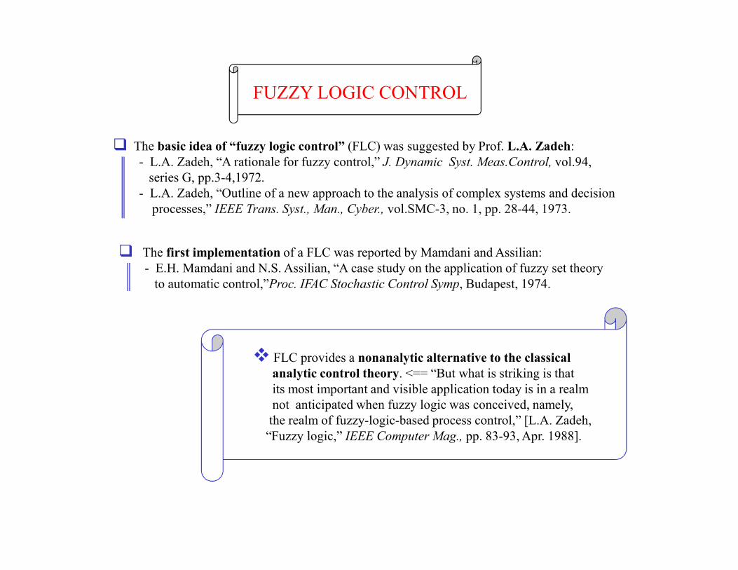
FUZZY LOGIC CONTROL

� The basic idea of “fuzzy logic control” (FLC) was suggested by Prof. L.A. Zadeh:

- L.A. Zadeh, “A rationale for fuzzy control,” J. Dynamic Syst. Meas.Control, vol.94,

series G, pp.3-4,1972.

- L.A. Zadeh, “Outline of a new approach to the analysis of complex systems and decision

processes,” IEEE Trans. Syst., Man., Cyber., vol.SMC-3, no. 1, pp. 28-44, 1973.

� The first implementation of a FLC was reported by Mamdani and Assilian:

- E.H. Mamdani and N.S. Assilian, “A case study on the application of fuzzy set theory

to automatic control,”Proc. IFAC Stochastic Control Symp, Budapest, 1974.

� FLC provides a nonanalytic alternative to the classical

analytic control theory. <== “But what is striking is that

its most important and visible application today is in a realm

not anticipated when fuzzy logic was conceived, namely,

the realm of fuzzy-logic-based process control,” [L.A. Zadeh,

“Fuzzy logic,” IEEE Computer Mag., pp. 83-93, Apr. 1988].

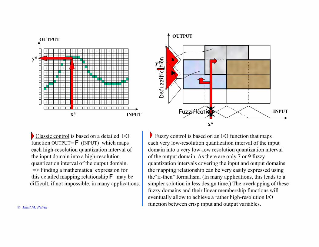
INPUT

OUTPUT

x*

y*

Classic control is based on a detailed I/O

function OUTPUT= F (INPUT) which maps

each high-resolution quantization interval of

the input domain into a high-resolution

quantization interval of the output domain.

=> Finding a mathematical expression for

this detailed mapping relationship F may be

difficult, if not impossible, in many applications.

INPUT

OUTPUT

Fuzzification

y*

x*

Defuzzification

Fuzzy control is based on an I/O function that maps

each very low-resolution quantization interval of the input

domain into a very low-low resolution quantization interval

of the output domain. As there are only 7 or 9 fuzzy

quantization intervals covering the input and output domains

the mapping relationship can be very easily expressed using

the“if-then” formalism. (In many applications, this leads to a

simpler solution in less design time.) The overlapping of these

fuzzy domains and their linear membership functions will

eventually allow to achieve a rather high-resolution I/O

function between crisp input and output variables.© Emil M. Petriu

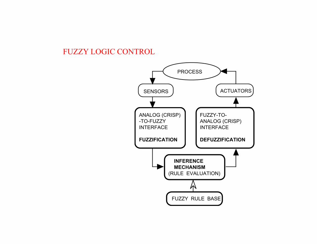
FUZZY LOGIC CONTROL

ANALOG (CRISP)

-TO-FUZZY

INTERFACE

FUZZIFICATION

FUZZY-TO-

ANALOG (CRISP)

INTERFACE

DEFUZZIFICATION

SENSORS ACTUATORS

INFERENCE

MECHANISM

(RULE EVALUATION)

FUZZY RULE BASE

PROCESS

∆/2−3∆/2 −∆/2 3∆/2∆−∆ 0

x

PZN

0

1

µN (x) , µZ (x), µP (x)

x*

µZ(x*)

µP(x*)

N =-1

∆/2

−3∆/2 −∆/2

3∆/2∆

−∆

0

XF

xZ=0

P =+1

Membership functions for

a 3-set fuzzy partition

Quantization characteristics

for the 3-set fuzzy partition

FUZZIFICATION

© Emil M. Petriu

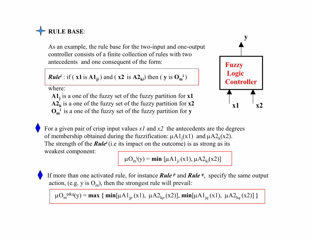
Fuzzy

Logic

Controller

x1 x2

yRULE BASE:

As an example, the rule base for the two-input and one-output

controller consists of a finite collection of rules with two

antecedents and one consequent of the form:

Rulei : if ( x1 is A1ji ) and ( x2 is A2ki) then ( y is Omi )

where:

A1j is a one of the fuzzy set of the fuzzy partition for x1

A2k is a one of the fuzzy set of the fuzzy partition for x2

Omi is a one of the fuzzy set of the fuzzy partition for y

For a given pair of crisp input values x1 and x2 the antecedents are the degrees

of membership obtained during the fuzzification: µA1j(x1) and µA2k(x2).

The strength of the Rulei (i.e its impact on the outcome) is as strong as its

weakest component:

µOmi(y) = min [µA1ji (x1), µA2ki(x2)]

If more than one activated rule, for instance Rule p and Rule q, specify the same output

action, (e.g. y is Om), then the strongest rule will prevail:

µOmp&q(y) = max { min[µA1jp (x1), µA2kp (x2)], min[µA1jq (x1), µA2kq (x2)] }

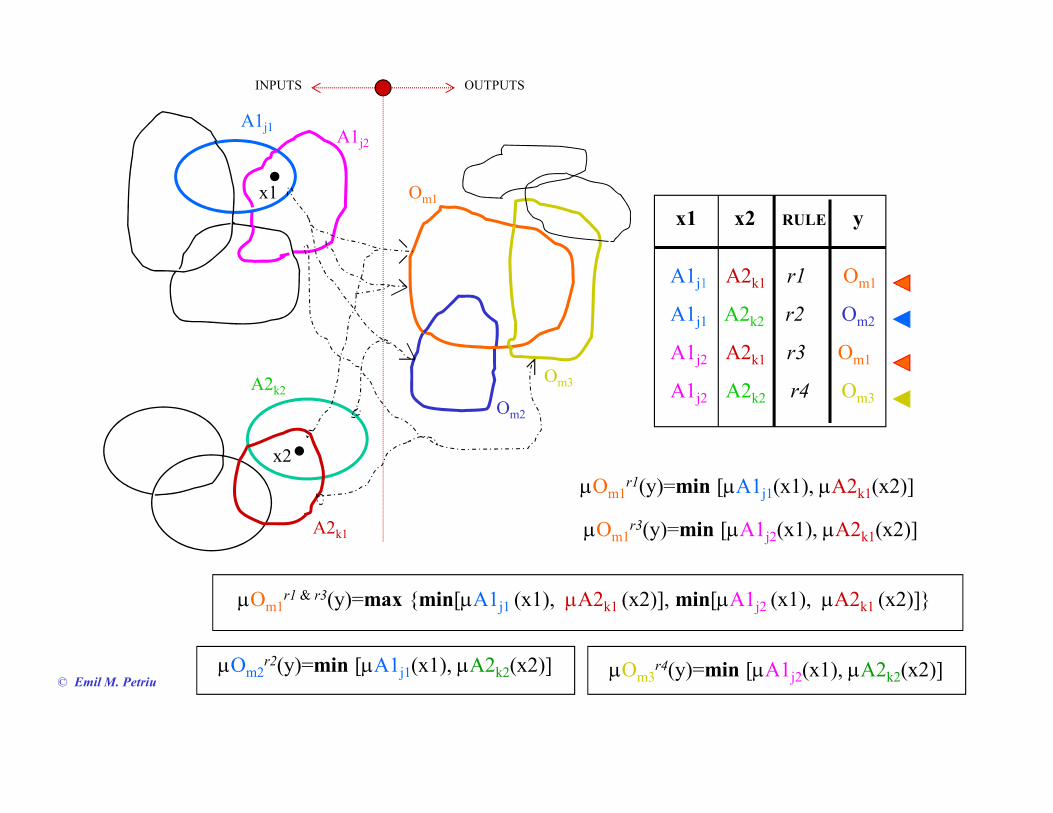
x1 x2 RULE y

A1j1 A2k1 r1 Om1

A1j1 A2k2 r2 Om2

A1j2 A2k1 r3 Om1

A1j2 A2k2 r4 Om3

µOm1r1(y)=min [µA1j1(x1), µA2k1(x2)]

µOm1r3(y)=min [µA1j2(x1), µA2k1(x2)]

µOm2r2(y)=min [µA1j1(x1), µA2k2(x2)] µOm3

r4(y)=min [µA1j2(x1), µA2k2(x2)]

µOm1r1 & r3(y)=max {min[µA1j1 (x1), µA2k1 (x2)], min[µA1j2 (x1), µA2k1 (x2)]}

x2

A2k1

A2k2

x1

A1j2

A1j1

Om2

Om1

Om3

INPUTS OUTPUTS

© Emil M. Petriu

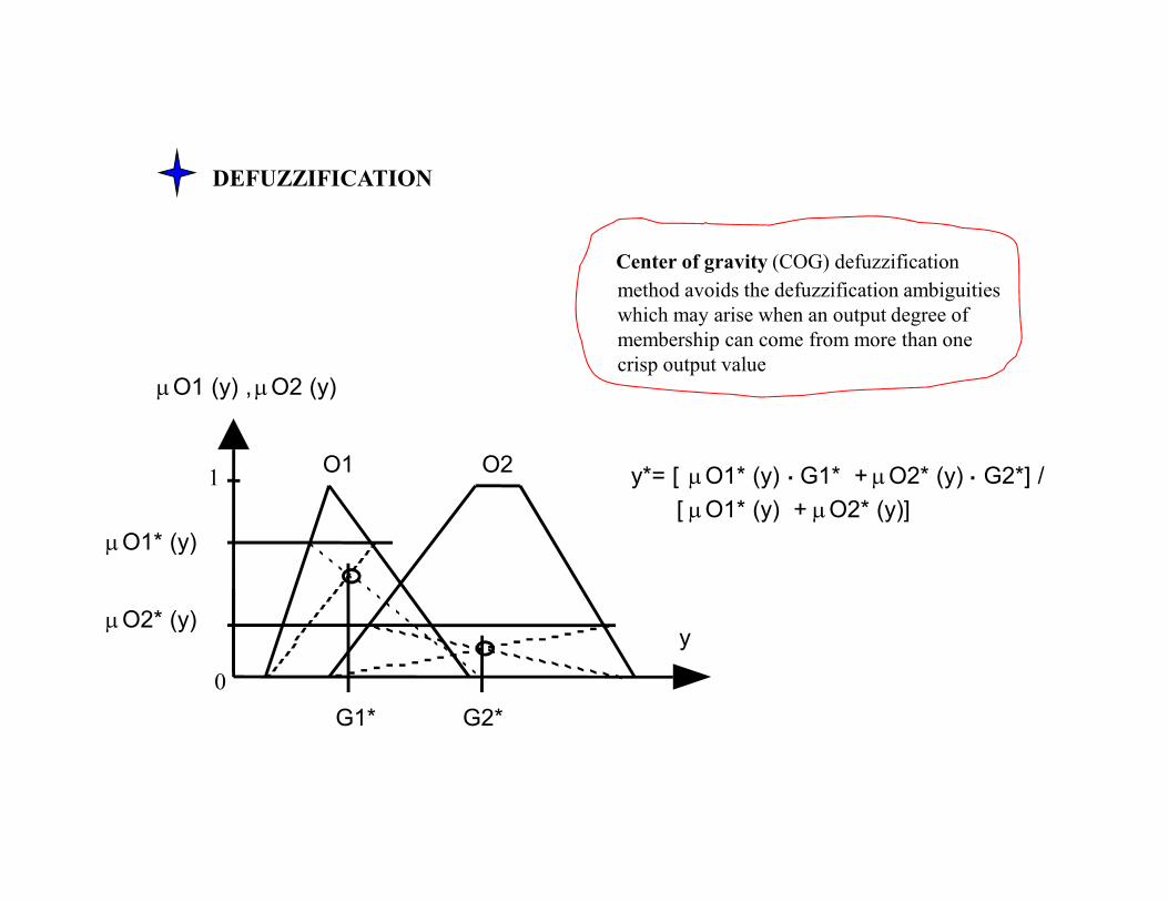
y

0

1

µO1 (y) , µO2 (y)

µO1* (y)

µO2* (y)

O1 O2

G1* G2*

y*= [ µO1* (y) G1* +

[ µO1* (y) + µO2* (y)]

. µO2* (y) G2*] / .

DEFUZZIFICATION

Center of gravity (COG) defuzzification

method avoids the defuzzification ambiguities

which may arise when an output degree of

membership can come from more than one

crisp output value

Fuzzy Controller for Truck and Trailer Docking

αθ

γ

DOCK

β

d

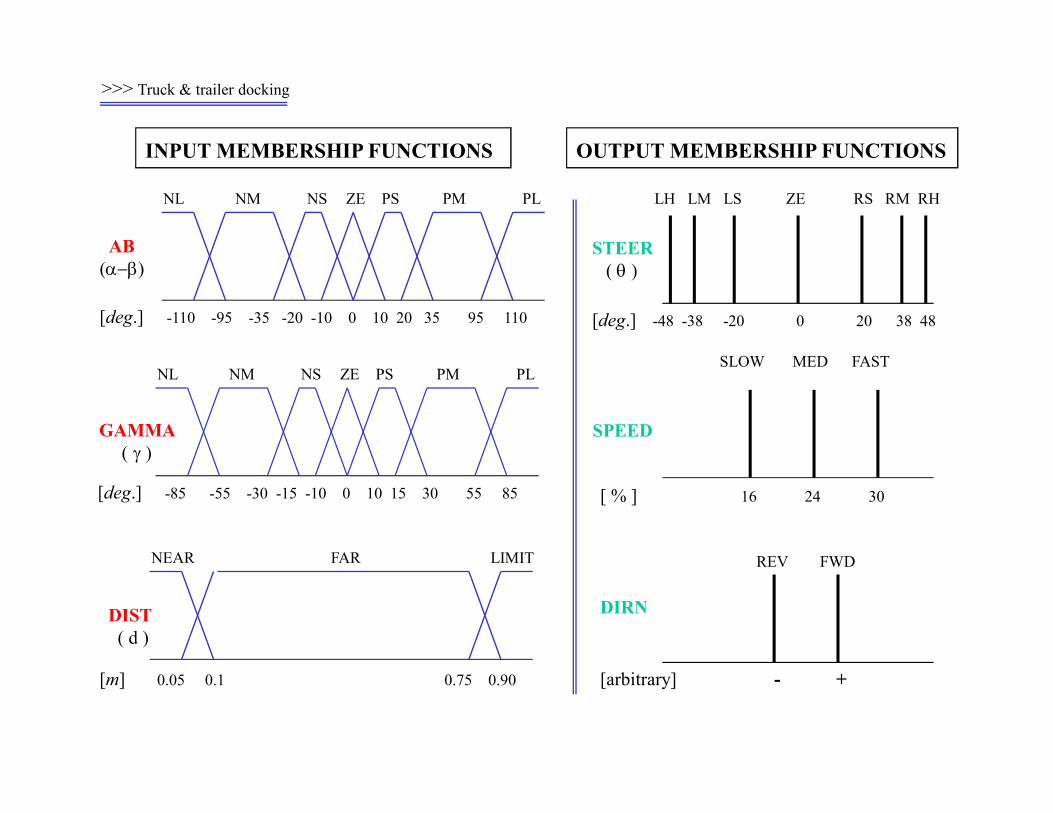
NL NM NS PS PM PLZE

AB

(α−β)

[deg.] -110 -95 -35 -20 -10 0 10 20 35 95 110

NL NM NS PS PM PLZE

GAMMA

( γ )

[deg.] -85 -55 -30 -15 -10 0 10 15 30 55 85

NEAR LIMITFAR

DIST

( d )

[m] 0.05 0.1 0.75 0.90

INPUT MEMBERSHIP FUNCTIONS

SPEED

[ % ] 16 24 30

STEER

( θ )

[deg.] -48 -38 -20 0 20 38 48

LH LM LS ZE RS RM RH

SLOW MED FAST

REV FWD

DIRN

[arbitrary] - +

OUTPUT MEMBERSHIP FUNCTIONS

>>> Truck & trailer docking

>>> Truck & trailer docking

STEER / DIRN

rule base

LM/F LS/F RS/F RM/F

LM ZE RM

RM

RH

RH

RHRM RH

RH/F

RH/F

RH/F

RH/F

RH/F

RH/FRH/FRH/FRM/F

LS/R RS/R

RS/R

RS/R RM/R

ZE/R

ZE PS PM PL

LH/F LH/F LH/F

LH

LH

LH

LM

LM

LH

ZE

LH/F

LH/F

LH/F

LH/F

LH/F

LM/F RS/FLS/F

LM/R

LS/R

LS/R

NM

NL

NS

ZE

PS

PM

PL

NL NM NS

GAMMA ( γ )

AB

(α−β)

F-R F-R F-R F-R F-R

F-R

F-R

F-R

F-R F-R F-R F-R F-R

F-R

F-R

F-R

There is a hysteresis ring around the

center of the rule base table for

the DIRN output. This means that when

the vehicle reaches a state within this

ring, it will continue to drive in the same

direction, F (forward) or R (reverse), as

it did in the previous state outside this ring.

The hysteresis was purposefully introduced

to increase the robustness of the FLC.

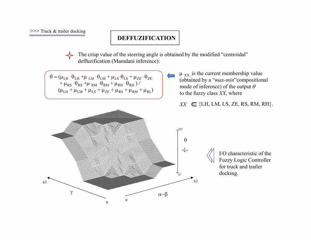
>>> Truck & trailer docking

DEFFUZIFICATION

The crisp value of the steering angle is obtained by the modified “centroidal”

deffuzification (Mamdani inference):

θ = (µLH. θLH +µ LM

. θLM + µLS. θLS + µZE

. θZE

+ µRS. θRS +µ RM

. θRM + µRH. θRH ) /

(µLH + µLM + µLS + µZE + µRS + µRM + µRL)

207

47

θ2

0

63

α−β

θ

63

γ

0

I/O characteristic of the

Fuzzy Logic Controller

for truck and trailer

docking.

µ XX is the current membership value

(obtained by a “max-min”compositional

mode of inference) of the output θto the fuzzy class XX, where

XX {LH, LM, LS, ZE, RS, RM, RH}.

U

There is tenet of common wisdom that FLCs are meant to successfully deal with uncertain data.

According to this, FLCs are supposed to make do with “uncertain” data coming from (cheap) low-resolution

and imprecise sensors. However, experiments show that the low resolution of the sensor data results in

rough quantization of of the controller's I/O characteristic:

207

47

θ20

63

α−β

θ

63

γ0

0

16

α−β

θ

16

γ0

207

47

θ1disp

4-bit

sensors7-bit

sensors

I/O characteristics of the FLC for truck & trailer docking for 4-bit sensor data (α, β, γ) and 7-bit sensor data.

“FUZZY UNCERTAINTY” ==> WHAT ACTUALLY IS “FUZZY” IN A FUZZY CONTROLLER ??

The key benefit of FLC is that the desired system behavior can be described with simple “if-then” relations

based on very low-resolution models able to incorporate empirical (i.e. not too “certain”?) engineering

knowledge. FLCs have found many practical applications in the context of complex ill-defined processes

that can be controlled by skilled human operators: water quality control, automatic train operation control,

elevator control, nuclear reactor control, automobile transmission control, etc., © Emil M. Petriu

Fuzzy Control for Backing-up a Four Wheel Truck

Using a truck backing-up Fuzzy Logic Controller (FLC) as test bed, this

Experiment revisits a tenet of common wisdom which considers FLCs

as beingmeant to make do with uncertain data coming from low-resolution

sensors.

The experiment studies the effects of the input sensor-data resolution on the

I/O characteristics of the digital FLC for backing-up a four-wheel truck.

Simulation experiments have shown that the low resolution of the sensor

data results in a rough quantization of the controller's I/O characteristic.

They also show that it is possible to smooth the I/O characteristic of a

digital FLC by dithering the sensor data before quantization.

ϕθ

d

Loading Dock

( , )x y Front Wheel

Back Wheel

(0,0)x

y

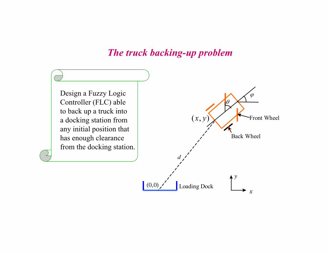
The truck backing-up problem

Design a Fuzzy Logic

Controller (FLC) able

to back up a truck into

a docking station from

any initial position that

has enough clearance

from the docking station.

0 4 5 15 20-4-5-15-20-5050

x-position

900 100080060030000-90 27001200 1500 1800

truck angle

00-250-350-450 250 350 450

LE LC CE RC RI

RB RU RV VE LV LU LB

NL NM NS ZE PS PM PL

ϕ

steering angle θ

0.0

1.0

1.0

0.0

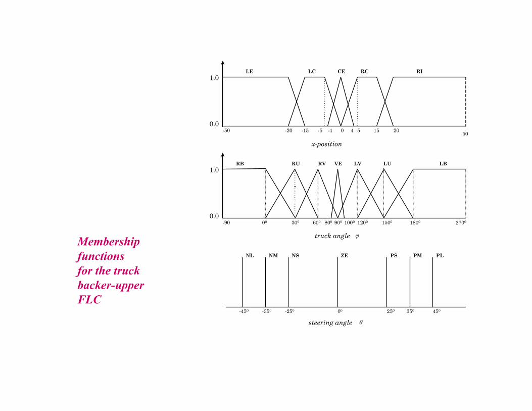
Membership

functions

for the truck

backer-upper

FLC

PS

NS

NM

NM

NL

NL

NL

PM PM

PM

PL PL

NL

NL

NM

NM

NS

PS

NM

NM

NS

PS

NM

NS

PS

PM

PM

PL

NS

PS

PM

PM

PL

PL

RL

RU

RV

VE

LV

LU

LL

LE LC CE RC RI

ϕ

x

ZE

1 2 3 4 5

6 7

18

31 35343332

30

The FLC is based

on the Sugeno-style

fuzzy inference.

The fuzzy rule base

consists of 35 rules.

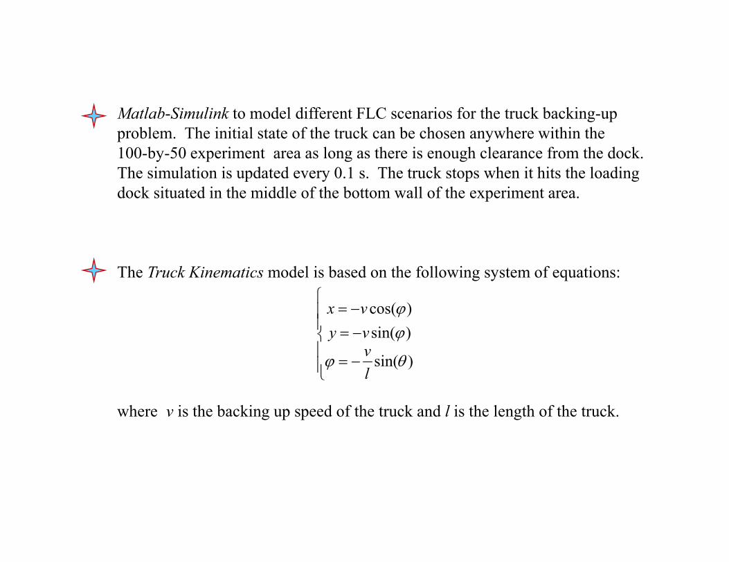
Matlab-Simulink to model different FLC scenarios for the truck backing-up

problem. The initial state of the truck can be chosen anywhere within the

100-by-50 experiment area as long as there is enough clearance from the dock.

The simulation is updated every 0.1 s. The truck stops when it hits the loading

dock situated in the middle of the bottom wall of the experiment area.

The Truck Kinematics model is based on the following system of equations:

where v is the backing up speed of the truck and l is the length of the truck.

−=

−=

−=

)sin(

)sin(

)cos(

θϕ

ϕϕ

l

v

vy

vx

u[2]<0

y<=0

Mux

XY Graph

TruckKinematics

theta_n.mat

To File

STOP

Stop

simulation

Scope1

Scope

InOut

Quantizer

Fuzzy Logic Controller

Variable Initialization

Demux

Demux2

DemuxDemux1

x

x

y

ϕθ

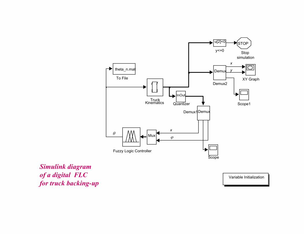
Simulink diagram

of a digital FLC

for truck backing-up

0 10 20 30 40 50 60 70-40

-30

-20

-10

0

10

20

30

Time (s)

θ [deg]

0 10 20 30 40 50 60-50

-40

-30

-20

-10

0

10

20

30

40

Time (s)

θ [deg]

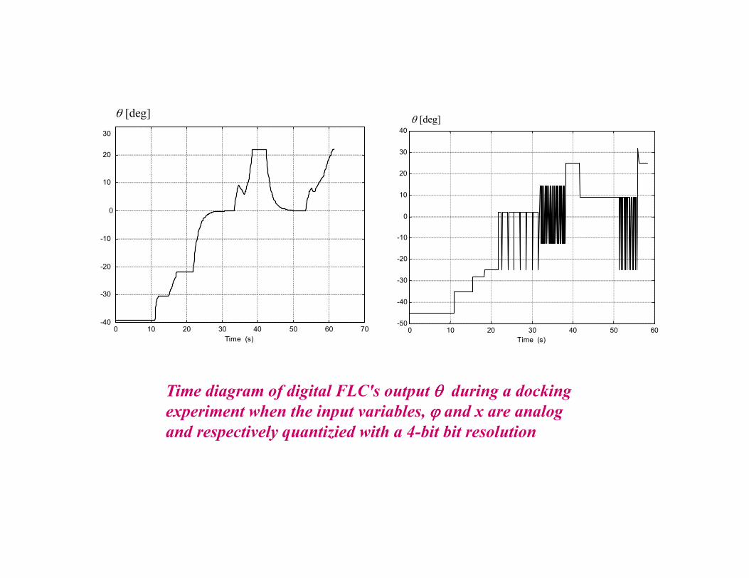
Time diagram of digital FLC's output θθθθ during a docking

experiment when the input variables, ϕϕϕϕ and x are analog

and respectively quantizied with a 4-bit bit resolution

A/D

A/D

∑

Dither

∑

Dither

Low-Pass

Filter

Low-Pass

Filter

Digital

FLC

Analog

Input

Analog

Input

Dithered

Analog Input

High Resolution

Digital Outputs

Dithered

Digital Input

Dithered

Digital Input

High Resolution

Digital Input

High Resolution

Digital Input

Dithered

Analog Input

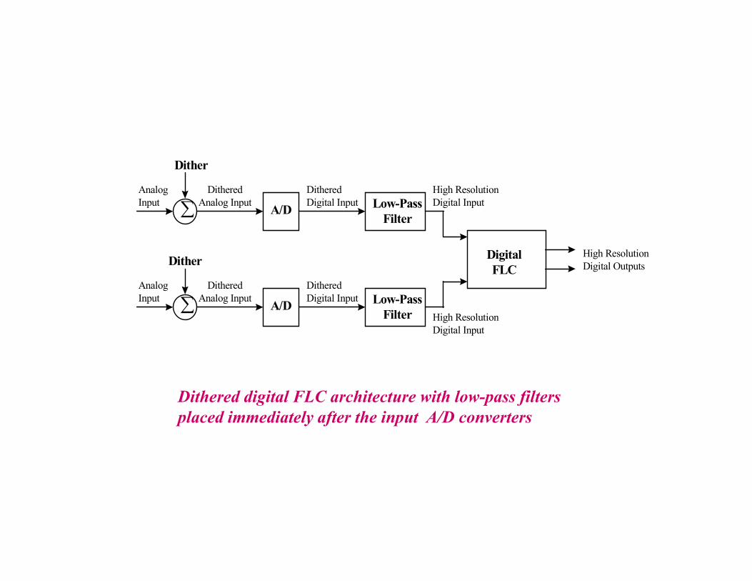
Dithered digital FLC architecture with low-pass filters

placed immediately after the input A/D converters

A/D

A/D

∑

Dither

∑

Dither

Low-Pass

Filter

Low-Pass

Filter

Digital

FLC

Analog

Input

Analog

Input

Dithered

Analog Input

High Resolution

Digital Output

Low-Resolution

Dithered Digital

Input

High Resolution

Digital Output

Low-Resolution

Dithered Digital

Input

Dithered

Analog Input

Dithered digital FLC architecture

with low-pass filters placed at the

FLC's outputs

It offers a better performance

than the previous one because

a final low-pass filter can also

smooth the non-linearity caused

by the min-max composition

rules of the FLC.

Time diagram of

dithered digital

FLC's output θ θ θ θ during a docking

experiment when

4-bit A/D converters

are used to quantize

the dithered inputs

and the low-pass

filter is placed at

the FLC's output

0 10 20 30 40 50 60 70-50

-40

-30

-20

-10

0

10

20

30

Θ [deg]

Time (s)

-50 50

0

10

20

30

40

50

X

Y

(a)

(b)

(c)

[dock]

initial position

(-30,25)

0

Truck trails for different FLC architectures: (a) analog ;

(b) digital without dithering; (c) digital with uniform

dithering and 20-unit moving average filter

Dithered FLCDigital FLC

Analog FLC

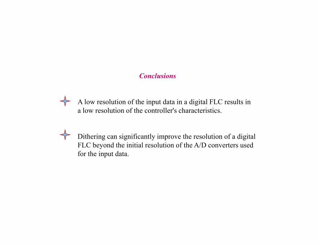
Conclusions

A low resolution of the input data in a digital FLC results in

a low resolution of the controller's characteristics.

Dithering can significantly improve the resolution of a digital

FLC beyond the initial resolution of the A/D converters used

for the input data.