Fuzzy Sets in Dynamic Adaptation of Parameters of a Bee ...

sensors

Article

Fuzzy Sets in Dynamic Adaptation of Parameters ofa Bee Colony Optimization for Controlling theTrajectory of an Autonomous Mobile Robot

Leticia Amador-Angulo 1,*, Olivia Mendoza 2, Juan R. Castro 2, Antonio Rodríguez-Díaz 2,Patricia Melin 1 and Oscar Castillo 1

1 Division of Graduate Studies and Research, Tijuana Institute of Technology, Tijuana 22414, Mexico;[email protected] (P.M.); [email protected] (O.C.)

2 Universidad Autónoma de Baja California, Tijuana 22390, Mexico; [email protected] (O.M.);[email protected] (J.R.C.); [email protected] (A.R.-D.)

* Correspondence: [email protected]; Tel.: +52-6642-856-236

Academic Editor: Dan ZhangReceived: 28 May 2016; Accepted: 29 August 2016; Published: 9 September 2016

Abstract: A hybrid approach composed by different types of fuzzy systems, such as the Type-1 FuzzyLogic System (T1FLS), Interval Type-2 Fuzzy Logic System (IT2FLS) and Generalized Type-2 FuzzyLogic System (GT2FLS) for the dynamic adaptation of the alpha and beta parameters of a Bee ColonyOptimization (BCO) algorithm is presented. The objective of the work is to focus on the BCO techniqueto find the optimal distribution of the membership functions in the design of fuzzy controllers. We useBCO specifically for tuning membership functions of the fuzzy controller for trajectory stability inan autonomous mobile robot. We add two types of perturbations in the model for the GeneralizedType-2 Fuzzy Logic System to better analyze its behavior under uncertainty and this shows betterresults when compared to the original BCO. We implemented various performance indices; ITAE,IAE, ISE, ITSE, RMSE and MSE to measure the performance of the controller. The experimentalresults show better performances using GT2FLS then by IT2FLS and T1FLS in the dynamic adaptationthe parameters for the BCO algorithm.

Keywords: bee colony optimization; fuzzy controller; fuzzy sets; uncertainty; dynamic adaptation;membership functions; perturbation; autonomous mobile robot

1. Introduction

In 1965 Zadeh first proposed the concept of a fuzzy set (FS) [1]. His vision was set on giving morecontrol over decision making, and with his fuzzy logic an immeasurable amount of decision- makingsituations could be easily modeled whereas hard logic, true or false, could not. This opened a newera in decision making with FSs that have been evolving since its initial days, first starting out withType-1 Fuzzy Logic Systems (T1FLS), then coming into Interval Type-2 Fuzzy Logic Systems (IT2FLS)and finally arriving to the current state of advanced form of FS, Generalized Type-2 Fuzzy LogicSystems (GT2FLS).

In recent years, many works on control system stabilization have been published [2–4]. However,all these control design methods require the exact mathematical models of the physical systems, whichmay not be available in practice. On the other hand, fuzzy control has been successfully applied forsolving many nonlinear control problems. Some works related in automatic control are [5–10]. Fuzzylogic or multi-valued logic is based on fuzzy set theory proposed in [1,11], which helps us in modelingknowledge, through the use of if-then rules. In Interval Type-2 fuzzy systems, the membershipfunctions can now return a range of values, which vary depending on the uncertainty involvedin not only the inputs, but also in the same membership functions [12,13]. In Generalized Type-2

Sensors 2016, 16, 1458; doi:10.3390/s16091458 www.mdpi.com/journal/sensors

http://www.mdpi.com/journal/sensors

http://www.mdpi.com

http://www.mdpi.com/journal/sensors

Sensors 2016, 16, 1458 2 of 27

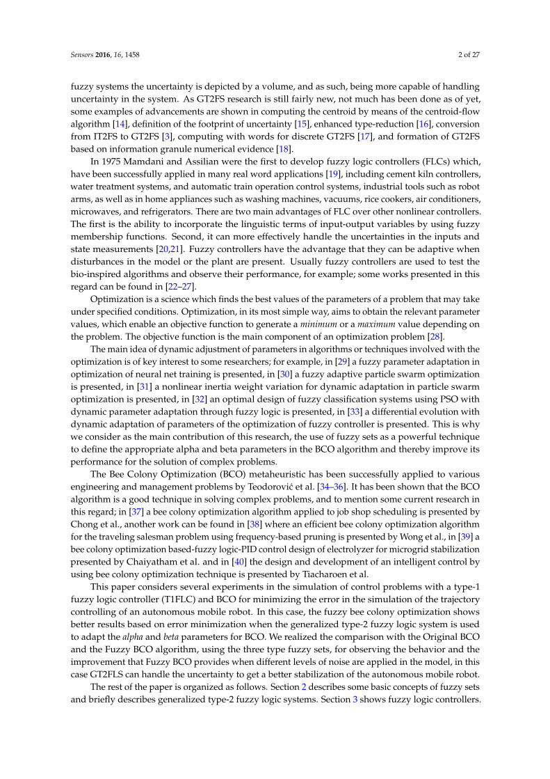
fuzzy systems the uncertainty is depicted by a volume, and as such, being more capable of handlinguncertainty in the system. As GT2FS research is still fairly new, not much has been done as of yet,some examples of advancements are shown in computing the centroid by means of the centroid-flowalgorithm [14], definition of the footprint of uncertainty [15], enhanced type-reduction [16], conversionfrom IT2FS to GT2FS [3], computing with words for discrete GT2FS [17], and formation of GT2FSbased on information granule numerical evidence [18].

In 1975 Mamdani and Assilian were the first to develop fuzzy logic controllers (FLCs) which,have been successfully applied in many real word applications [19], including cement kiln controllers,water treatment systems, and automatic train operation control systems, industrial tools such as robotarms, as well as in home appliances such as washing machines, vacuums, rice cookers, air conditioners,microwaves, and refrigerators. There are two main advantages of FLC over other nonlinear controllers.The first is the ability to incorporate the linguistic terms of input-output variables by using fuzzymembership functions. Second, it can more effectively handle the uncertainties in the inputs andstate measurements [20,21]. Fuzzy controllers have the advantage that they can be adaptive whendisturbances in the model or the plant are present. Usually fuzzy controllers are used to test thebio-inspired algorithms and observe their performance, for example; some works presented in thisregard can be found in [22–27].

Optimization is a science which finds the best values of the parameters of a problem that may takeunder specified conditions. Optimization, in its most simple way, aims to obtain the relevant parametervalues, which enable an objective function to generate a minimum or a maximum value depending onthe problem. The objective function is the main component of an optimization problem [28].

The main idea of dynamic adjustment of parameters in algorithms or techniques involved with theoptimization is of key interest to some researchers; for example, in [29] a fuzzy parameter adaptation inoptimization of neural net training is presented, in [30] a fuzzy adaptive particle swarm optimizationis presented, in [31] a nonlinear inertia weight variation for dynamic adaptation in particle swarmoptimization is presented, in [32] an optimal design of fuzzy classification systems using PSO withdynamic parameter adaptation through fuzzy logic is presented, in [33] a differential evolution withdynamic adaptation of parameters of the optimization of fuzzy controller is presented. This is whywe consider as the main contribution of this research, the use of fuzzy sets as a powerful techniqueto define the appropriate alpha and beta parameters in the BCO algorithm and thereby improve itsperformance for the solution of complex problems.

The Bee Colony Optimization (BCO) metaheuristic has been successfully applied to variousengineering and management problems by Teodorovic et al. [34–36]. It has been shown that the BCOalgorithm is a good technique in solving complex problems, and to mention some current research inthis regard; in [37] a bee colony optimization algorithm applied to job shop scheduling is presented byChong et al., another work can be found in [38] where an efficient bee colony optimization algorithmfor the traveling salesman problem using frequency-based pruning is presented by Wong et al., in [39] abee colony optimization based-fuzzy logic-PID control design of electrolyzer for microgrid stabilizationpresented by Chaiyatham et al. and in [40] the design and development of an intelligent control byusing bee colony optimization technique is presented by Tiacharoen et al.

This paper considers several experiments in the simulation of control problems with a type-1fuzzy logic controller (T1FLC) and BCO for minimizing the error in the simulation of the trajectorycontrolling of an autonomous mobile robot. In this case, the fuzzy bee colony optimization showsbetter results based on error minimization when the generalized type-2 fuzzy logic system is usedto adapt the alpha and beta parameters for BCO. We realized the comparison with the Original BCOand the Fuzzy BCO algorithm, using the three type fuzzy sets, for observing the behavior and theimprovement that Fuzzy BCO provides when different levels of noise are applied in the model, in thiscase GT2FLS can handle the uncertainty to get a better stabilization of the autonomous mobile robot.

The rest of the paper is organized as follows. Section 2 describes some basic concepts of fuzzy setsand briefly describes generalized type-2 fuzzy logic systems. Section 3 shows fuzzy logic controllers.

Sensors 2016, 16, 1458 3 of 27

Section 4 outlines the problem statement that is used in the simulations. Section 5 describes thetraditional bee colony optimization (BCO) algorithm and fuzzy BCO. Section 6 shows the simulationresults with the dynamic adaptation in the parameters of BCO with different fuzzy systems. Section 7shows the discussion of results. Finally, Section 8 offers some conclusions of this work.

2. Fuzzy Sets

2.1. Type-1 Fuzzy Logic System

A type-1 fuzzy set in the universe X is characterized by a membership function µA (x)taking values on the interval [0, 1] and can be represented as a set of ordered pairs of anelement and the membership degree of an element to the set and are defined by the followingEquation (1) [1,4,20,21,41,42]:

A = (x,µA (x)) | x ∈ X (1)

where µA : X→ [0, 1] .In this definition µA (x) represents the membership degree of the element x ∈ X to the set A.

In this work we are going the use the following notation: A (x) = µA (x) for all x ∈ X. Figure 1 showsthe Type-1 Fuzzy Logic System.

Sensors 2016, 16, 1458 3 of 28

simulation results with the dynamic adaptation in the parameters of BCO with different fuzzy systems. Section 7 shows the discussion of results. Finally, Section 8 offers some conclusions of this work.

2. Fuzzy Sets

2.1. Type-1 Fuzzy Logic System

A type-1 fuzzy set in the universe X is characterized by a membership function ( ) taking values on the interval [0, 1] and can be represented as a set of ordered pairs of an element and the membership degree of an element to the set and are defined by the following Equation (1) [1,4,20,21,41,42]: A = (x, μ (x)) | x ∈ X (1)

where μ : X → [0,1]. In this definition μ (x) represents the membership degree of the element x ∈ X to the set A. In

this work we are going the use the following notation: A(x) = μ (x) for all x ∈ X. Figure 1 shows the Type-1 Fuzzy Logic System.

Figure 1. Type-1 fuzzy logic system.

2.2. Interval Type-2 Fuzzy Logic System

Based on Zadeh’s ideas, Mendel et al. presented the mathematical definition of a type-2 fuzzy set, as follows [20,21].

An Interval Type-2 Fuzzy Set A, denoted by μ (x) and μ (x) is represented by the lower and upper membership functions of μ (x). Where x ∈ X. In this case, Equation (2) shows the definition of an IT2FS [43–49]: A = (x, u), 1 | ∀x ∈ X, ∀u ∈ J ⊆ [0,1] (2)

where X is the primary domain, Jx is the secondary domain. All secondary degrees (μ (x, u)) are equal to 1. Figure 2 shows the representation of an Interval Type-2 Fuzzy Logic System.

The output processor includes a type-reducer and defuzzifier that generates a type-1 fuzzy set output (from the type-reducer) or a crisp number (from the defuzzifier) [46,49]. An Interval type-2 FLS is also characterized by IF-THEN rules, but their fuzzy sets are now of interval type-2 form. The Type-2 Fuzzy Set can be used when circumstances are too uncertain to determine exact membership degrees, as is the case with the membership functions in a fuzzy controller that can take different values and we want to find the distribution of membership functions that show better results in the stability of the fuzzy controller [50,51].

Figure 1. Type-1 fuzzy logic system.

2.2. Interval Type-2 Fuzzy Logic System

Based on Zadeh’s ideas, Mendel et al. presented the mathematical definition of a type-2 fuzzy set,as follows [20,21].

An Interval Type-2 Fuzzy Set A, denoted by µA(x) and µA(x) is represented by the lower andupper membership functions of µA (x). Where x ∈ X. In this case, Equation (2) shows the definitionof an IT2FS [43–49]:

A = ((x, u) , 1) | ∀x ∈ X, ∀u ∈ Jx ⊆ [0, 1] (2)

where X is the primary domain, Jx is the secondary domain. All secondary degrees(µA (x, u)

)are

equal to 1. Figure 2 shows the representation of an Interval Type-2 Fuzzy Logic System.The output processor includes a type-reducer and defuzzifier that generates a type-1 fuzzy set

output (from the type-reducer) or a crisp number (from the defuzzifier) [46,49]. An Interval type-2 FLSis also characterized by IF-THEN rules, but their fuzzy sets are now of interval type-2 form. The Type-2Fuzzy Set can be used when circumstances are too uncertain to determine exact membership degrees,as is the case with the membership functions in a fuzzy controller that can take different values andwe want to find the distribution of membership functions that show better results in the stability of thefuzzy controller [50,51].

Sensors 2016, 16, 1458 4 of 27Sensors 2016, 16, 1458 4 of 28

Figure 2. Interval Type-2 fuzzy logic system.

2.3. Generalized Type-2 Fuzzy Logic System

With GT2FLS the logic is generally the same as for T1FLS and IT2FLS, but their operations are somewhat different, due to the nature of GT2FS [51,52]. Generalized Type-2 Fuzzy Sets are defined by the following Equation (3): A = (x, u), μ (x, u) | ∀x ∈ X, ∀u ∈ J ⊆ [0,1] (3)

where J ⊆ [0, 1], x is the partition of the primary membership function, and u is the partition of the secondary membership function. In Figure 3 we can find a representation of a generalized type-2 membership function, and in Figure 4, the footprint of uncertainty (FOU) is illustrated, which is associated with the third dimension and allows a better modeling of real world uncertainty.

Figure 3. Generalized Type-2 membership function.

Figure 4. FOU of the Generalized Type-2 membership function.



With GT2FLS the logic is generally the same as for T1FLS and IT2FLS, but their operations aresomewhat different, due to the nature of GT2FS [51,52]. Generalized Type-2 Fuzzy Sets are defined bythe following Equation (3):

˜A =(

(x, u) ,µA (x, u))| ∀x ∈ X, ∀u ∈ Jx ⊆ [0, 1]

(3)

where Jx ⊆ [0, 1], x is the partition of the primary membership function, and u is the partition of thesecondary membership function. In Figure 3 we can find a representation of a generalized type-2membership function, and in Figure 4, the footprint of uncertainty (FOU) is illustrated, which isassociated with the third dimension and allows a better modeling of real world uncertainty.

Sensors 2016, 16, 1458 4 of 28






Figure 4. FOU of the Generalized Type-2 membership function.


Sensors 2016, 16, 1458 4 of 28






Figure 4. FOU of the Generalized Type-2 membership function. Figure 4. FOU of the Generalized Type-2 membership function.

Sensors 2016, 16, 1458 5 of 27

It must be noted that there is a small difference in notation when compared with Type-1 andInterval Type-2, this is, T1FS and IT2FS use the notation µ (x) , but GT2FS uses fx (u), in the verticalaxis, and this is due to the complexity involved in GT2FLS in comparison with the others, as wellas how GT2FLS has been described in the literature [53]. Figure 5 shows the representation of aGeneralized Type-2 Fuzzy Logic System.

Sensors 2016, 16, 1458 5 of 28

It must be noted that there is a small difference in notation when compared with Type-1 and Interval Type-2, this is, T1FS and IT2FS use the notation μ(x), but GT2FS uses f (u), in the vertical axis, and this is due to the complexity involved in GT2FLS in comparison with the others, as well as how GT2FLS has been described in the literature [53]. Figure 5 shows the representation of a Generalized Type-2 Fuzzy Logic System.

Figure 5. Generalized Type-2 fuzzy logic system.

2.3.1. Fuzzification

The fuzzifier maps crisp inputs into generalized type-2 fuzzy sets to process within the FLC. In this paper, we will focus on the type-2 singleton fuzzifier as it is fast to compute and, thus, suitable for the generalized type-2 FLC real-time operation. Singleton fuzzification maps the crisp input into a fuzzy set, which has a single point of nonzero membership. Hence, the singleton fuzzifier maps the crisp input x into a type-2 fuzzy singleton, whose MF is = 1/1 for = and = 0 for all ≠ for all = 1, 2, . . . , , where P is the number of FLS inputs [54].

2.3.2. Inference

Once the input and output variables are defined, with their respective membership functions, the inference process is performed in the system, and for this the following steps are needed:

Define the Fuzzy Rules: The structure of the rules in the generalized Type-2 FLS is the standard Mamdani-type FLS rule structure used in the Type-1 FLS and an interval Type-2 FLS, but in this paper, we assume that the antecedents and the consequents sets are represented by generalized Type-2 fuzzy sets. So for a Type-2 FLS with p inputs x ϵX , … , x ∈ X and one output y ∈ Y, Multiple Input Single Output (MISO), if we assume there are M rules, the kth rule in the generalized type-2 FLS can be written as follows [52–54]: : IF is and…and is , THEN is (4)

The inference of a GT2FLS can be simplified into two main operations, meet and join, as shown in Equations (5) and (6), respectively

Figure 5. Generalized Type-2 fuzzy logic system.

2.3.1. Fuzzification

The fuzzifier maps crisp inputs into generalized type-2 fuzzy sets to process within the FLC.In this paper, we will focus on the type-2 singleton fuzzifier as it is fast to compute and, thus, suitablefor the generalized type-2 FLC real-time operation. Singleton fuzzification maps the crisp input into afuzzy set, which has a single point of nonzero membership. Hence, the singleton fuzzifier maps thecrisp input x′p into a type-2 fuzzy singleton, whose MF is µAp

(xp)= 1/1 for xp = x′p and µAp

(xp)= 0

for all xp 6= x′p for all p = 1, 2, . . . , P, where P is the number of FLS inputs [54].

2.3.2. Inference

Once the input and output variables are defined, with their respective membership functions,the inference process is performed in the system, and for this the following steps are needed:

Define the Fuzzy Rules: The structure of the rules in the generalized Type-2 FLS is the standardMamdani-type FLS rule structure used in the Type-1 FLS and an interval Type-2 FLS, but in this paper,we assume that the antecedents and the consequents sets are represented by generalized Type-2 fuzzysets. So for a Type-2 FLS with p inputs x1 ε X1, . . . , xp ∈ XP and one output y ∈ Y, Multiple InputSingle Output (MISO), if we assume there are M rules, the kth rule in the generalized type-2 FLS canbe written as follows [52–54]:

Rk : IF x1 is Fk1 and . . . and xp is Fk

p , THEN y is Gk (4)

Sensors 2016, 16, 1458 6 of 27

The inference of a GT2FLS can be simplified into two main operations, meet and join, as shown inEquations (5) and (6), respectively

µA(x, u) t µB(x, w)= (v, fx(u)∗ fx(w)) | v ∈ u ∨ w, u ∈ Jux ⊆ [0, 1], w ∈ Jw

x ⊆ [0, 1] (5)

µA(x, u) u µB(x, w)= (v, fx(u)∗ fx(w)) | v ∈ u∧w, u ∈ Jux ⊆ [0, 1], w ∈ Jw

x ⊆ [0, 1] (6)

2.3.3. α-Planes Representation

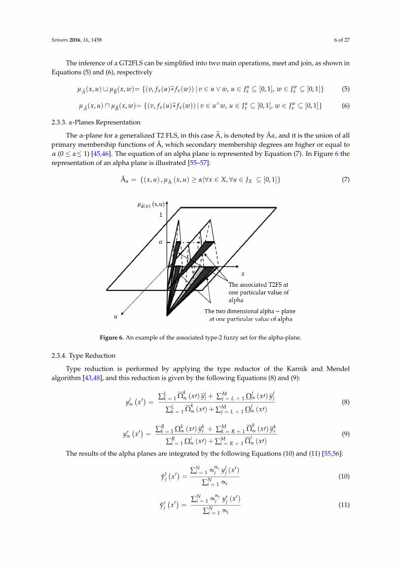
The α-plane for a generalized T2 FLS, in this case A, is denoted by Ãα, and it is the union of allprimary membership functions of Ã, which secondary membership degrees are higher or equal toα (0 ≤ α≤ 1) [45,46]. The equation of an alpha plane is represented by Equation (7). In Figure 6 therepresentation of an alpha plane is illustrated [55–57]:

Ãα = (x, u) , µÃ (x, u) ≥ α|∀x ∈ X, ∀u ∈ JX ⊆ [0, 1] (7)

Sensors 2016, 16, 1458 6 of 28

),(~ uxA

⊔ ),(~ wxB

]1,0[],1,0[,|))(*~

)(,( wx

uxxx JwJuwuvwfufv (5)

),(~ uxA

⊓ ?B (x,w) ]1,0[],1,0[,^|))(*

~)(,( w

xuxxx JwJuwuvwfufv (6)

2.3.3. α-Planes Representation

The α-plane for a generalized T2 FLS, in this case A, is denoted by Ãα, and it is the union of all primary membership functions of Ã, which secondary membership degrees are higher or equal to α (0 ≤ α≤ 1) [45,46]. The equation of an alpha plane is represented by Equation (7). In Figure 6 the representation of an alpha plane is illustrated [55–57]: Ã = ( , ), Ã( , ) ≥ |∀ ∈ , ∀ ∈ ⊆ [0,1] (7)

Figure 6. An example of the associated type-2 fuzzy set for the alpha-plane.

2.3.4. Type Reduction

Type reduction is performed by applying the type reductor of the Karnik and Mendel algorithm [43,48], and this reduction is given by the following Equations (8) and (9):

∝( ) = ∑ Ω∝( ′) + ∑ Ω∝( ′) ∑ Ω∝( ′) + ∑ Ω∝( ′) (8)

∝ ′ =∑ Ω∝( ′) + ∑ Ω∝( ′) ∑ Ω∝( ′) + ∑ Ω∝( ′) (9)

The results of the alpha planes are integrated by the following Equations (10) and (11) [55,56]: ŷ ( ) = ∑ ∝∝ ( )∑ ∝ (10)

ŷ ( ) = ∑ ∝∝ ( )∑ ∝ (11)

Figure 6. An example of the associated type-2 fuzzy set for the alpha-plane.

2.3.4. Type Reduction

Type reduction is performed by applying the type reductor of the Karnik and Mendelalgorithm [43,48], and this reduction is given by the following Equations (8) and (9):

yl∝(

x′)=

∑Lk = 1 Ωk

∝ (x′) yil + ∑M

j = L + 1 Ωj∝ (x′) yj

l

∑Lk = 1 Ωk

∝ (x′) + ∑Mj = L + 1 Ωj

∝ (x′)(8)

yr∝(

x′)=

∑Rk = 1 Ωk

∝ (x′) ykr + ∑M

k = R + 1 Ωk∝ (x′) yk

r

∑Ri = 1 Ωi

∝ (x′) + ∑Mi = R + 1 Ωi

∝ (x′)(9)

The results of the alpha planes are integrated by the following Equations (10) and (11) [55,56]:

ylj(

x′)=

∑Ni = 1 ∝∝i

i ylj (x′)

∑Ni = 1 ∝i

(10)

yrj(

x′)=

∑Ni = 1 ∝∝i

i yrj (x′)

∑Ni = 1 ∝i

(11)

Sensors 2016, 16, 1458 7 of 27

2.3.5. Defuzzification

After realizing the type reduction and integrating the results of all the alpha planes,the defuzzification is performed by using the average of yl and yr, to obtain the defuzzified output ofa generalized type-2 non-singleton FLS [58,59]:

yj(

x′)=

ylj (x′) + yr

j (x′)

2(12)

3. Fuzzy Controllers

Early, a Fuzzy Logic Controller (FLC) was designed only using type-1 fuzzy sets in representingthe input-output uncertainties. However, these are uncertainties in the meaning of words in theantecedents and consequents of the rules, the histogram values of the consequents extracted from agroup of experts, and the noisy data as well as measurements [2–4,33,41,42,59]. Type-1 fuzzy sets havelimited ability to handle such uncertainties because they apply crisp membership functions. In Figure 7the generic representation of the FLC is illustrated.

Sensors 2016, 16, 1458 7 of 28


After realizing the type reduction and integrating the results of all the alpha planes, the defuzzification is performed by using the average of and , to obtain the defuzzified output of a generalized type-2 non-singleton FLS [58,59]: ŷ ( ) = ŷ ( ) + ŷ ( )2 (12)


Early, a Fuzzy Logic Controller (FLC) was designed only using type-1 fuzzy sets in representing the input-output uncertainties. However, these are uncertainties in the meaning of words in the antecedents and consequents of the rules, the histogram values of the consequents extracted from a group of experts, and the noisy data as well as measurements [2–4,33,41,42,59]. Type-1 fuzzy sets have limited ability to handle such uncertainties because they apply crisp membership functions. In Figure 7 the generic representation of the FLC is illustrated.

Figure 7. General representation of a FLC.

4. Problem Statement

4.1. General Description

The model which is used is of a unicycle mobile robot [2–4,42,59], consisting of two driving wheels located on the same axis and a front free wheel. Figure 8 shows a graphical description of the robot model.

Figure 8. Mobile robot model.




The model which is used is of a unicycle mobile robot [2–4,42,59], consisting of two drivingwheels located on the same axis and a front free wheel. Figure 8 shows a graphical description of therobot model.

Sensors 2016, 16, 1458 7 of 28


After realizing the type reduction and integrating the results of all the alpha planes, the defuzzification is performed by using the average of and , to obtain the defuzzified output of a generalized type-2 non-singleton FLS [58,59]: ŷ ( ) = ŷ ( ) + ŷ ( )2 (12)


Early, a Fuzzy Logic Controller (FLC) was designed only using type-1 fuzzy sets in representing the input-output uncertainties. However, these are uncertainties in the meaning of words in the antecedents and consequents of the rules, the histogram values of the consequents extracted from a group of experts, and the noisy data as well as measurements [2–4,33,41,42,59]. Type-1 fuzzy sets have limited ability to handle such uncertainties because they apply crisp membership functions. In Figure 7 the generic representation of the FLC is illustrated.




The model which is used is of a unicycle mobile robot [2–4,42,59], consisting of two driving wheels located on the same axis and a front free wheel. Figure 8 shows a graphical description of the robot model.

Figure 8. Mobile robot model. Figure 8. Mobile robot model.

Sensors 2016, 16, 1458 8 of 27

The robot model assumes that the motion of the free wheel can be ignored in its dynamics,as shown in Equations (13) and (14):

M (q).v + C

(q,

.q)

v + Dv = τ + P (t) (13)

where:

q = (x, y, θ)T is the vector of the configuration coordinates,υ = (v, w)T is the vector of velocities,τ = (τ1, τ2) is the vector of torques applied to the wheels of the robot where τ1 and τ2 denote thetorques of the right and left wheel, respectively.P ∈ R2 is the uniformly bounded disturbance vector,M (q) ∈ R2×2 is the positive-definite inertia matrix,C(q,

.q)

ϑ is the vector of centripetal and Coriolis forces, andD ∈ R2×2 is a diagonal positive-definite damping matrix.

The kinematic system is represented by Equation (14):

.q =

cos θ

sin θ

0

001

︸︷︷︸

J(q)

[vw

]︸︷︷︸

υ

(14)

where:

(x,y) is the position in the X − Y (world) reference frame,θ is the angle between the heading direction and the x-axis,v and w are the linear and angular velocities.

Furthermore, Equation (15) shows the non-holonomic constraint which this system has, whichcorresponds to a no-slip wheel condition preventing the robot from moving sideways:

.ycosθ − .

xsinθ = 0 (15)

The system fails to meet Brockett’s necessary condition for feedback stabilization, which impliesthat no continuous static state-feedback controller exists that can stabilize the closed-loop systemaround the equilibrium point.

4.2. Characteristics of the Fuzzy Controller

The main problem to study is controlling the stability of the trajectory in a mobile robot.The Membership functions are for the two inputs to the fuzzy system: the first is called ev (angularvelocity), which has three membership functions with linguistic values of N (Negative), Z (Zero)and P (Positive). The second input variable is called ew (linear velocity) with three membershipfunctions with the same linguistic values. The type-1 fuzzy logic controller has two outputs called T1(Torque 1), and T2 (Torque 2), which are composed of three triangular membership functions with thefollowing linguistic values, respectively: N (Negative), Z (Zero), P (Positive), and in Figure 9 we showthe representation of the input and output variables.


Figure 9. Characteristics of the Type-1 FLC of the mobile robot controller.

Table 1. Fuzzy Rules used by the Fuzzy Controller.

# Rules Input 1 Input 2 Output 1 Output 2

ev ew T1 T2 1 N N N N 2 N Z N Z 3 N P N P 4 Z N Z N 5 Z Z Z Z 6 Z P Z P 7 P N P N 8 P Z P Z 9 P P P P

Angular velocity (ev) and negative and linear velocity (ew).

Figure 9. Characteristics of the Type-1 FLC of the mobile robot controller.

The knowledge about the problem provides us with nine fuzzy rules for control. The combinationof the rules is shown in Table 1 and Figure 10 shows the model of the Fuzzy Logic Controller.

Table 1. Fuzzy Rules used by the Fuzzy Controller.

# RulesInput 1 Input 2 Output 1 Output 2

ev ew T1 T2

1 N N N N2 N Z N Z3 N P N P4 Z N Z N5 Z Z Z Z6 Z P Z P7 P N P N8 P Z P Z9 P P P P

Angular velocity (ev) and negative and linear velocity (ew).

The rules are selected based on the following references [3,4,59]. We choose the initial FIS withthe nine rules set out in Table 1. For example, the third rule; when the angular velocity (ev) is Negativeand linear velocity (ew) is Positive then the output Torque 1 (T1—Wheel right) is Negative (it indicatesno movement) and Torque 2 (T2—Wheel left) is Positive (it indicates movement). Each torque hasindependent functions with a direct relationship that depending on the ev and ew values.

Sensors 2016, 16, 1458 10 of 27Sensors 2016, 16, x 10 of 28

Figure 10. Fuzzy controller of the autonomous mobile robot.Figure 10. Fuzzy controller of the autonomous mobile robot.

Sensors 2016, 16, 1458 11 of 27

5. Bee Colony Optimization

The Bee Colony Optimization algorithm has recently received many improvements andapplications. The BCO algorithm mimics the food foraging behavior of swarms of honey bees [35].Honey bees use several mechanisms like the waggle dance to optimally locate a food source and searchfor new ones. It is a very simple, robust and population based stochastic optimization algorithm [36].

5.1. Traditional Bee Colony Optimization Algorithm

The communication between individual insects in a colony of social insects has been well known.The BCO is inspired by the bees´ behavior in nature. The basic idea behind the BCO is to createthe multi agent system (colony of artificial bees) capable to successfully solve difficult combinatorialoptimization problems. The artificial bee colony behaves partially alike, and partially differently frombee colonies in nature [34–40,42]. The algorithm parameters, whose values need to be set prior thealgorithm execution are; B indicates the number of bees in the hive and NC indicates the number ofconstructive moves during one forward pass. In the beginning of the search, all the bees are in the hive.

The basic steps of the BCO algorithm are shown in Table 2. The BCO algorithm is based onEquations (16)–(19):

Pij,n =[ρij,n]

α.[ 1dij]β

∑j ∈ Ai,n

[ρij,n]α.[ 1

dij]β

(16)

Di = K.P fi

P fcolony(17)

P fi =1LI

, Li = Tour Length (18)

P fcolony =1

NBee

NBee

∑i = 1

P fi (19)

Table 2. Basic Steps of the BCO Algorithm.

Pseudocode of BCO

1. Initialization: an empty solution is assigned to every bee;2. For every bee: //the forward pass

(a) Set k = 1; //counter for constructive moves in the forward pass;(b) Evaluate all possible constructive moves;(c) According to evaluation, choose on move using the roulette wheel;(d) k = k + 1; if k ≤ NC goto step b.

3. All bees are back to the hive; //backward pass starts.4. Evaluate (partial) objective function value for each bee;5. Every bee decide randomly whether to continue its own exploration and become a recruiter, or to

become a follower;6. For every follower, choose a new solution from recruiters by the roulette wheel;7. If solutions are not completed goto step 2;8. Evaluate all solutions and find the best one;9. If stopping condition is not met goto step 2;

10. Output the best solution found.

Equation (16) indicates the probability of a bee k located on a node i selects the next node denotedby j, where, Nki is the set of feasible nodes (in a neighborhood) connected to node i with respect to beek, and ρij is the probability to visit the following node. Note that the β is inversely proportional to the

Sensors 2016, 16, 1458 12 of 27

distance of the node; dij represents the distance of node i until node j, for this algorithm indicate thetotal the dance that a bee have in this moment. Finally, α is a binary variable that is used to find bettersolutions in the algorithm. Equation (17) represents that a waggle dance will last for a certain duration,determined by a linear function, where K denotes the waggle dance scaling factor, Pfi denotes theprofitability scores of bee i as defined in Equation (18) and Pfcolony denotes the bee colony’s averageprofitability as in Equation (19) and is updated after each bee completes its tour. For this research thewaggle dance is represented by the mean square error (MSE), which it is the representation of thefitness function in the fuzzy control analyzed, for each iteration in BCO algorithm a MSE is found, themain objective is to find the smallest error can stabilize the trajectory of an autonomous mobile robot.In the BCO algorithm, a bee represents the values of the distribution of the membership functions.The design of the T1FLS for the mobile robot controller has trapezoidal and triangular membershipfunctions in the inputs and outputs (see Figure 9), giving a total of 40 values.

5.2. Fuzzy Bee Colony Optimization Algorithm

In the BCO algorithm the waggle dance represents the intensity with which a bee finds a possiblegood solution. If the intensity of the waggle dance is large this means that the solution found bythe bee is the best of all the population [60]. For this work the waggle dance is represented by themean square error (MSE) that all models find once the simulation in the iteration of the algorithm isdone [41,42]. For measuring the iterations of the algorithm, it was decided to use the percentage ofiterations as a variable, i.e., when starting the algorithm the iterations will be considered “low”, andwhen the iterations are completed it will be considered “high” or close to 100%. We represent this ideausing Equation (20) [32]:

Iteration =Current Iteration

Maximum of Iterations(20)

The diversity measure is defined by Equation (21), which measures the degree of dispersion of thebees, i.e., when the bees are closer together; there is less diversity as well as when bees are separatedthen the diversity is higher. As the reader will realize the equation of diversity can be considered asthe average of the Euclidean distances between each bee and the best bee. The main objective of usingdiversity is to provide the BCO algorithm with the ability to avoid getting trapped in local minimum;this is because the diversity represents the situation when the bees are not separated in the searchspace. This behavior is controlled with the rules that were designed with the Generalized Type-2 FuzzyLogic System [32]:

Diversity(S(t)) =1ns

nx

∑i = 1

√Xij(t)− X j(t))2 (21)

where t indicates the current iteration, ns indicates the size of the population, i represents the bee,nx indicates the number of solutions, j represents the next solution in the space search, Xij indicatessolution j of the bee i, finally, Xj represents solution j of the best bee in the space search.

The fitness function in the BCO algorithm is calculated with the Mean Square Error and is shownin Equation (22). For each Follower Bee for N cycles, the Type-1 FLS design for the BCO algorithm isevaluated and the objective is to minimize the error:

MSE =1n

n

∑i = 1

(Yi −Yi)2 (22)

The distribution of the membership functions in the inputs and outputs is realized in a symmetricalway. The design of the input and output variables can be appreciated in Figures 11–13 for the Type-1FLS, Interval Type-2 FLS and Generalized Type-2 FLS, respectively. The fuzzy rules are shownin Table 3.

Sensors 2016, 16, 1458 13 of 27

Sensors 2016, 16, 1458 13 of 28

where t indicates the current iteration, indicates the size of the population, i represents the bee, indicates the number of solutions, j represents the next solution in the space search, indicates

solution j of the bee i, finally, j represents solution j of the best bee in the space search. The fitness function in the BCO algorithm is calculated with the Mean Square Error and is shown

in Equation (22). For each Follower Bee for N cycles, the Type-1 FLS design for the BCO algorithm is evaluated and the objective is to minimize the error:

2

1

1( )

n

i ii

MSE Y Yn

(22)

The distribution of the membership functions in the inputs and outputs is realized in a symmetrical way. The design of the input and output variables can be appreciated in Figures 11–13 for the Type-1 FLS, Interval Type-2 FLS and Generalized Type-2 FLS, respectively. The fuzzy rules are shown in Table 3.

Figure 11. Fuzzy BCO with T1FLS. Figure 11. Fuzzy BCO with T1FLS.

Sensors 2016, 16, 1458 14 of 28

Figure 12. Fuzzy BCO with IT2FLS.

Table 3. Rules for the Fuzzy BCO with dynamic adaptation of the beta and alpha parameter values.

# Rules Input 1 Input 2 Output Output

Iteration Diversity Beta Alpha 1 Low Low High Low 2 Low Medium MediumHigh Medium 3 Low High MediumHigh MediumLow 4 Medium Low MediumHigh MediumLow 5 Medium Medium Medium Medium 6 Medium High MediumLow MediumHigh 7 High Low Medium High 8 High Medium MediumLow MediumHigh 9 High High Low High

Figure 12. Fuzzy BCO with IT2FLS.


Figure 13. Fuzzy BCO with GT2FLS.

Various experiments were previously realized in which the idea is to explore the behavior of the BCO algorithm. The interesting factor that was found is that we need to start with high exploration and thus, the proposed methodology is able to analyze better all the search space.

To start the BCO algorithm, the iteration is low and the diversity is low, this is because the initialization of the position of the bees is set randomly in steps 1 of the BCO algorithm. This reasoning that is used for realizing the Rule number 1 which is: “If Iterations is Low and Diversity is Low then Beta is High and Alpha is Low”. The high value for beta represents that the bees should realize high exploration and the value low of alpha represents that the bees should have little exploitation in BCO algorithm. On the other hand, when the Iterations are high (last iterations of the BCO algorithm) the bees have a high diversity (bees are separated) and the value of beta is low to obtain low exploration and the value of alpha is high to obtain a better exploitation in the problem. This reasoning is used for realizing Rule number 9, which is: “If Iterations is High and Diversity is High then Beta is Low and Alpha is High”.

The proposed general flowchart of BCO is illustrated in Figure 14, where “ScoutBees” indicates the size of population, “NC” represents the number of constructive moves during one forward pass and “FollowerBees” represents each bee that explores the possible solutions.

Figure 13. Fuzzy BCO with GT2FLS.

Table 3. Rules for the Fuzzy BCO with dynamic adaptation of the beta and alpha parameter values.

# RulesInput 1 Input 2 Output Output

Iteration Diversity Beta Alpha

1 Low Low High Low2 Low Medium MediumHigh Medium3 Low High MediumHigh MediumLow4 Medium Low MediumHigh MediumLow5 Medium Medium Medium Medium6 Medium High MediumLow MediumHigh7 High Low Medium High8 High Medium MediumLow MediumHigh9 High High Low High

Various experiments were previously realized in which the idea is to explore the behavior of theBCO algorithm. The interesting factor that was found is that we need to start with high explorationand thus, the proposed methodology is able to analyze better all the search space.

To start the BCO algorithm, the iteration is low and the diversity is low, this is because theinitialization of the position of the bees is set randomly in steps 1 of the BCO algorithm. This reasoningthat is used for realizing the Rule number 1 which is: “If Iterations is Low and Diversity is Low then Beta isHigh and Alpha is Low”. The high value for beta represents that the bees should realize high explorationand the value low of alpha represents that the bees should have little exploitation in BCO algorithm.On the other hand, when the Iterations are high (last iterations of the BCO algorithm) the bees have ahigh diversity (bees are separated) and the value of beta is low to obtain low exploration and the valueof alpha is high to obtain a better exploitation in the problem. This reasoning is used for realizing Rulenumber 9, which is: “If Iterations is High and Diversity is High then Beta is Low and Alpha is High”.

Sensors 2016, 16, 1458 15 of 27

The proposed general flowchart of BCO is illustrated in Figure 14, where “ScoutBees” indicatesthe size of population, “NC” represents the number of constructive moves during one forward passand “FollowerBees” represents each bee that explores the possible solutions.Sensors 2016, 16, 1458 16 of 28

Figure 14. Flowchart of the proposed Fuzzy BCO.

6. Results

Experimentation was performed with various external perturbation scenarios. Two specific noise generators are used: band-limited white noise and pulse generated noise. The height of the Power Spectral Density of the band-limited white noise of power is set to (0.5, 1), sample time of (0.5, 1), and delay of 1000; and the amplitude is set to (0.5, 1), period in seconds of 1, pulse width (%) is set to (0.5, 1) and phase delay is set to 1000, respectively, for the pulse generated noise.

We use the problem of controlling a trajectory of an autonomous mobile robot, the test criteria is a series of Performance Indices; where the Integral Square Error (ISE), Integral Absolute Error (IAE), Integral Time Squared Error (ITSE), Integral Time Absolute Error (ITAE) and Root Mean Square Error (RMSE) are used, respectively shown in Equations (23)–(27):

0

2 dtteISE (23)

0

dtteIAE (24)

0

2 tdtteITSE (25)

Figure 14. Flowchart of the proposed Fuzzy BCO.

6. Results

Experimentation was performed with various external perturbation scenarios. Two specific noisegenerators are used: band-limited white noise and pulse generated noise. The height of the PowerSpectral Density of the band-limited white noise of power is set to (0.5, 1), sample time of (0.5, 1),and delay of 1000; and the amplitude is set to (0.5, 1), period in seconds of 1, pulse width (%) is set to(0.5, 1) and phase delay is set to 1000, respectively, for the pulse generated noise.

We use the problem of controlling a trajectory of an autonomous mobile robot, the test criteria is aseries of Performance Indices; where the Integral Square Error (ISE), Integral Absolute Error (IAE),Integral Time Squared Error (ITSE), Integral Time Absolute Error (ITAE) and Root Mean Square Error(RMSE) are used, respectively shown in Equations (23)–(27):

ISE =

∞∫0

e2 (t) dt (23)

IAE =

∞∫0

|e (t)| dt (24)

Sensors 2016, 16, 1458 16 of 27

ITSE =

∞∫0

e2 (t) tdt (25)

ITAE =

∞∫0

|e (t)| tdt (26)

ε =

√√√√ 1N

N

∑t = 1

(Xt − Xt)

2

(27)

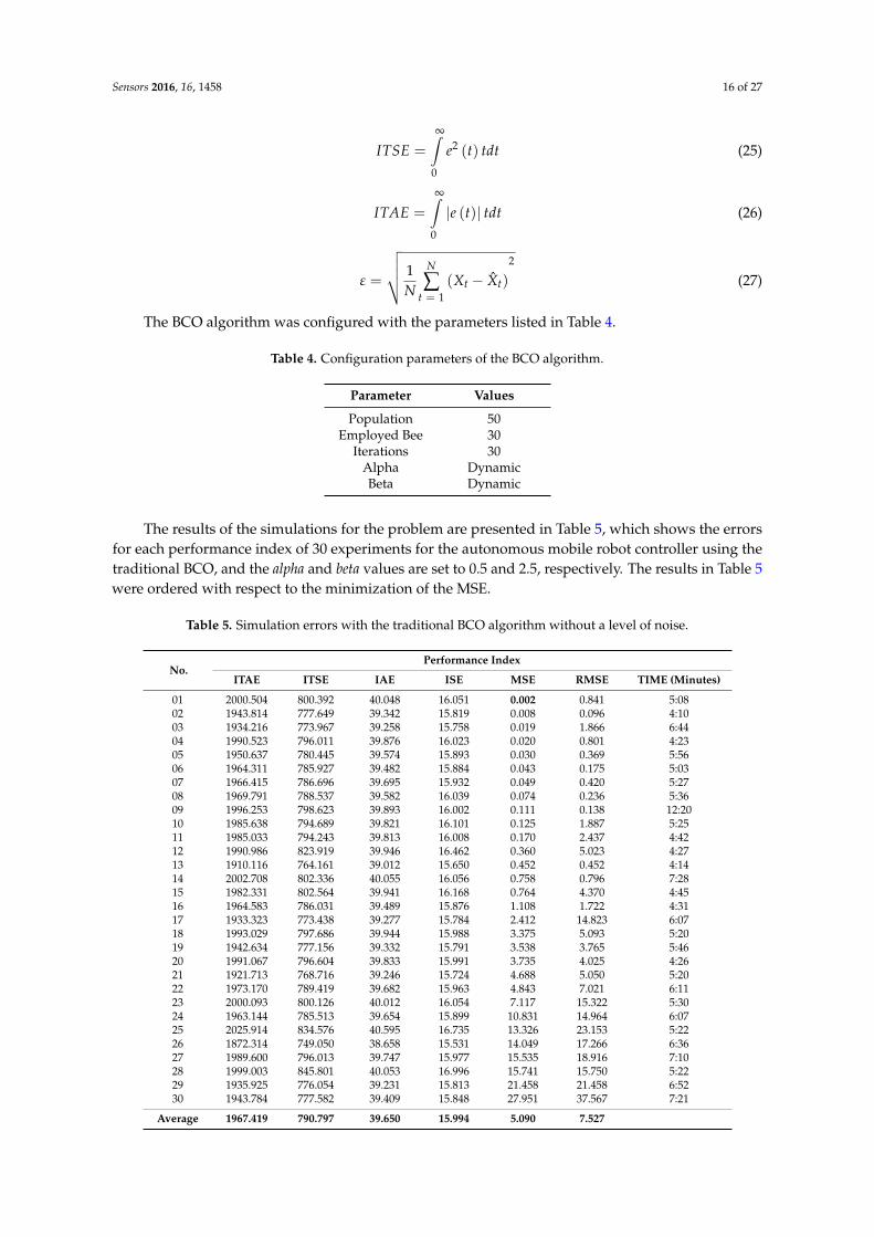
The BCO algorithm was configured with the parameters listed in Table 4.

Table 4. Configuration parameters of the BCO algorithm.

Parameter Values

Population 50Employed Bee 30

Iterations 30Alpha DynamicBeta Dynamic

The results of the simulations for the problem are presented in Table 5, which shows the errorsfor each performance index of 30 experiments for the autonomous mobile robot controller using thetraditional BCO, and the alpha and beta values are set to 0.5 and 2.5, respectively. The results in Table 5were ordered with respect to the minimization of the MSE.

Table 5. Simulation errors with the traditional BCO algorithm without a level of noise.

No.Performance Index

ITAE ITSE IAE ISE MSE RMSE TIME (Minutes)

01 2000.504 800.392 40.048 16.051 0.002 0.841 5:0802 1943.814 777.649 39.342 15.819 0.008 0.096 4:1003 1934.216 773.967 39.258 15.758 0.019 1.866 6:4404 1990.523 796.011 39.876 16.023 0.020 0.801 4:2305 1950.637 780.445 39.574 15.893 0.030 0.369 5:5606 1964.311 785.927 39.482 15.884 0.043 0.175 5:0307 1966.415 786.696 39.695 15.932 0.049 0.420 5:2708 1969.791 788.537 39.582 16.039 0.074 0.236 5:3609 1996.253 798.623 39.893 16.002 0.111 0.138 12:2010 1985.638 794.689 39.821 16.101 0.125 1.887 5:2511 1985.033 794.243 39.813 16.008 0.170 2.437 4:4212 1990.986 823.919 39.946 16.462 0.360 5.023 4:2713 1910.116 764.161 39.012 15.650 0.452 0.452 4:1414 2002.708 802.336 40.055 16.056 0.758 0.796 7:2815 1982.331 802.564 39.941 16.168 0.764 4.370 4:4516 1964.583 786.031 39.489 15.876 1.108 1.722 4:3117 1933.323 773.438 39.277 15.784 2.412 14.823 6:0718 1993.029 797.686 39.944 15.988 3.375 5.093 5:2019 1942.634 777.156 39.332 15.791 3.538 3.765 5:4620 1991.067 796.604 39.833 15.991 3.735 4.025 4:2621 1921.713 768.716 39.246 15.724 4.688 5.050 5:2022 1973.170 789.419 39.682 15.963 4.843 7.021 6:1123 2000.093 800.126 40.012 16.054 7.117 15.322 5:3024 1963.144 785.513 39.654 15.899 10.831 14.964 6:0725 2025.914 834.576 40.595 16.735 13.326 23.153 5:2226 1872.314 749.050 38.658 15.531 14.049 17.266 6:3627 1989.600 796.013 39.747 15.977 15.535 18.916 7:1028 1999.003 845.801 40.053 16.996 15.741 15.750 5:2229 1935.925 776.054 39.231 15.813 21.458 21.458 6:5230 1943.784 777.582 39.409 15.848 27.951 37.567 7:21

Average 1967.419 790.797 39.650 15.994 5.090 7.527

Sensors 2016, 16, 1458 17 of 27

In Table 5 can be noted that the best value for the MSE was of 0.002. The simulation results inTable 5 are obtained with the traditional BCO. The main goal of the experiments is to observe thevalues of alpha and beta in the algorithm to compare with the results of the proposed method, as wellas to observe the results with the traditional BCO algorithm with the considered problem. Figure 15shows the behavior of the MSE when different levels of noise are applied in the traditional BCO.

Sensors 2016, 16, 1458 18 of 28

22 1973.170 789.419 39.682 15.963 4.843 7.021 6:11 23 2000.093 800.126 40.012 16.054 7.117 15.322 5:30 24 1963.144 785.513 39.654 15.899 10.831 14.964 6:07 25 2025.914 834.576 40.595 16.735 13.326 23.153 5:22 26 1872.314 749.050 38.658 15.531 14.049 17.266 6:36 27 1989.600 796.013 39.747 15.977 15.535 18.916 7:10 28 1999.003 845.801 40.053 16.996 15.741 15.750 5:22 29 1935.925 776.054 39.231 15.813 21.458 21.458 6:52 30 1943.784 777.582 39.409 15.848 27.951 37.567 7:21

Average 1967.419 790.797 39.650 15.994 5.090 7.527

Figure 15. Behavior of the traditional BCO with different perturbation in the model.

With the base FLS the distribution of membership functions detailed in Figure 9. The behavior in the simulations is shown in Figure 16 with a perturbation in the model of pulse generated with value of 1.

Figure 16. Trajectory in the autonomous mobile robot controller with base FLS with perturbation in the model.


With the base FLS the distribution of membership functions detailed in Figure 9. The behaviorin the simulations is shown in Figure 16 with a perturbation in the model of pulse generated withvalue of 1.

Sensors 2016, 16, 1458 18 of 28

22 1973.170 789.419 39.682 15.963 4.843 7.021 6:11 23 2000.093 800.126 40.012 16.054 7.117 15.322 5:30 24 1963.144 785.513 39.654 15.899 10.831 14.964 6:07 25 2025.914 834.576 40.595 16.735 13.326 23.153 5:22 26 1872.314 749.050 38.658 15.531 14.049 17.266 6:36 27 1989.600 796.013 39.747 15.977 15.535 18.916 7:10 28 1999.003 845.801 40.053 16.996 15.741 15.750 5:22 29 1935.925 776.054 39.231 15.813 21.458 21.458 6:52 30 1943.784 777.582 39.409 15.848 27.951 37.567 7:21

Average 1967.419 790.797 39.650 15.994 5.090 7.527


With the base FLS the distribution of membership functions detailed in Figure 9. The behavior in the simulations is shown in Figure 16 with a perturbation in the model of pulse generated with value of 1.

Figure 16. Trajectory in the autonomous mobile robot controller with base FLS with perturbation in the model.

Figure 16. Trajectory in the autonomous mobile robot controller with base FLS with perturbation inthe model.

Figure 17 shows similar simulation errors when the levels of noise are applied in the model,the stabilization in the trajectory in autonomous mobile robot is shown in Figure 17 with the best MSEusing the two types of perturbations in the model with the value of 1 and the traditional BCO.

Sensors 2016, 16, 1458 18 of 27

Sensors 2016, 16, 1458 19 of 28

Figure 17 shows similar simulation errors when the levels of noise are applied in the model, the stabilization in the trajectory in autonomous mobile robot is shown in Figure 17 with the best MSE using the two types of perturbations in the model with the value of 1 and the traditional BCO.

Figure 17. Trajectory in the autonomous mobile robot controller, (a)Traditional BCO; (b) BCO algorithm applied perturbation called band-limited with value of 1; (c) BCO algorithm applied perturbation called pulse generator with value of 1.

Table 6 shows the average of 30 experiments, standard deviation (SD), the best and the worst of the simulation errors for the four methods: Traditional BCO, Fuzzy BCO with Type-1 Fuzzy Logic System (FLS), Fuzzy BCO with Interval Type-2 FLS and Fuzzy BCO with Generalized Type-2 FLS without applying perturbation in the model. We used the MSE as the fitness function in the Bee Colony Optimization algorithm.

Table 6. Simulation results without perturbation in the model.

Performance Index

Methods

Traditional BCO

Fuzzy BCO with Type-1

FLS

Fuzzy BCO with Interval Type-2 FLS

Fuzzy BCO with Generalized Type-2 FLS

ITAE 1967.419 1834.635 1890.023 1918.058 ITSE 790.797 744.277 773.802 779.201 IAE 39.650 37.054 38.416 38.918 ISE 15.994 15.098 15.770 15.887

MSE 5.090 2.599 4.059 6.118 RMSE 7.527 5.416 7.385 8.352

MSE Standard Deviation 7.276 3.322 5.965 13.000

Figure 17. Trajectory in the autonomous mobile robot controller, (a)Traditional BCO; (b) BCO algorithmapplied perturbation called band-limited with value of 1; (c) BCO algorithm applied perturbationcalled pulse generator with value of 1.

Table 6 shows the average of 30 experiments, standard deviation (SD), the best and the worst ofthe simulation errors for the four methods: Traditional BCO, Fuzzy BCO with Type-1 Fuzzy LogicSystem (FLS), Fuzzy BCO with Interval Type-2 FLS and Fuzzy BCO with Generalized Type-2 FLSwithout applying perturbation in the model. We used the MSE as the fitness function in the Bee ColonyOptimization algorithm.

Table 6 shows that using the traditional method the average MSE was of 5.090 and withGeneralized Type-2 FLS was 6.118 using the dynamic adjustment in alpha and beta, which tells us thatif we do not apply perturbation in the model the dynamic adjustment do not provide better resultscompared to the traditional BCO for the stabilization of the autonomous mobile robot. The alphaand beta values found by Fuzzy BCO with GT2FLS are 2.601 and 0.467, respectively. We appliedperturbation in the model, and this is a way of analyzing uncertainty in the fuzzy sets. Table 7 showsresults with the pulse generator with a value of 0.5 for each methodology used.

Sensors 2016, 16, 1458 19 of 27

Table 6. Simulation results without perturbation in the model.

Performance Index

Methods

TraditionalBCO

Fuzzy BCOwith Type-1

FLS

Fuzzy BCOwith IntervalType-2 FLS

Fuzzy BCO withGeneralizedType-2 FLS

ITAE 1967.419 1834.635 1890.023 1918.058

ITSE 790.797 744.277 773.802 779.201

IAE 39.650 37.054 38.416 38.918

ISE 15.994 15.098 15.770 15.887

MSE 5.090 2.599 4.059 6.118

RMSE 7.527 5.416 7.385 8.352

MSE

Standard Deviation 7.276 3.322 5.965 13.000

Best 0.002 0.004 0.006 0.003

Worst 27.951 13.132 24.411 66.507

Beta 2.5 (Fixed) 3.074 2.599 2.601

Alpha 0.5 (Fixed) 0.661 0.466 0.467

Table 7. Simulation results with pulse generator perturbation in the model.

Performance Index

Methods

TraditionalBCO

Fuzzy BCOwith Type-1

FLS

Fuzzy BCOwith IntervalType-2 FLS

Fuzzy BCO withGeneralizedType-2 FLS

ITAE 1974.966 1951.805 1893.691 1895.279

ITSE 795.631 785.731 762.295 759.013

IAE 39.340 37.545 38.242 38.269

ISE 16.110 15.945 15.456 15.380

MSE 2.601 3.490 3.361 2.467

RMSE 4.460 7.478 6.750 8.149

MSE

Standard Deviation 3.764 4.875 4.122 8.313

Best 0.018 0.001 0.034 0.007

Worst 14.048 23.393 4.122 40.853

Beta 2.5(Fixed) 2.992 2.812 2.601

Alpha 0.5(Fixed) 0.784 0.494 0.467

Table 7 shows that using the traditional method with perturbation in the model the average MSEwas 2.601 and with Generalized Type-2 FLS was 2.467 using the dynamic adjustment in alpha and betavalues, which tells us that if we apply perturbation in the model the dynamic adjustment producesbetter results compared to the traditional BCO for the stabilization of the autonomous mobile robot.The minimum value of MSE was 0.001 for the Fuzzy BCO with Type-1 FLS. The best alpha and betavalues found by GT2FLS are 2.601 and 0.467, respectively.

Figure 18 shows comparative results when applying a pulse generator with a value of 1 in themodel. The MSE is shown for comparison.


Figure 18. Comparative results of each method with different perturbation in the model.

Figure 19. Behavior of various performance indices in relation to band-limited perturbations with value of 1 presents the system, when Fuzzy Bee Colony Optimization-Type-1 Fuzzy Logic System, FBCO-Interval Type-2 Fuzzy Logic System and FBCO-Generalized Type-2 Fuzzy Logic System are used. (a) ITAE; (b) ITSE; (c) IAE; and (d) ISE.


Figure 18 shows that the best error is found by GT2FLS with a value of 0.0001. It is important tomention that GT2FLS starts with a low error, but the stabilization in the trajectory of the autonomousmobile robot is high compared to other methods.

As an example of the relation between noise and the FLS performance, Figure 19 shows theserelations for each type of performance index used, where in all accounts FBCO with GT2FLS issomewhat better with respect to Fuzzy BCO with IT2FLS and then to Fuzzy BCO with T1FLS.

Sensors 2016, 16, 1458 21 of 28


Figure 19. Behavior of various performance indices in relation to band-limited perturbations with value of 1 presents the system, when Fuzzy Bee Colony Optimization-Type-1 Fuzzy Logic System, FBCO-Interval Type-2 Fuzzy Logic System and FBCO-Generalized Type-2 Fuzzy Logic System are used. (a) ITAE; (b) ITSE; (c) IAE; and (d) ISE.

Figure 19. Behavior of various performance indices in relation to band-limited perturbations withvalue of 1 presents the system, when Fuzzy Bee Colony Optimization-Type-1 Fuzzy Logic System,FBCO-Interval Type-2 Fuzzy Logic System and FBCO-Generalized Type-2 Fuzzy Logic System areused. (a) ITAE; (b) ITSE; (c) IAE; and (d) ISE.

Sensors 2016, 16, 1458 21 of 27

Two scenarios in the experiments were changed, the first is to observe the behavior of the IntervalType-2 FLS, a reduction in the size of the Footprint Uncertainty (FOU) to a value of 0.5 was realized.In experiments previously performed, the value of FOU was set to 0.9. The second is to minimize thevalue of the FOU to 0.5 and also, increase the value of the volume (depth) of a generalized membershipfunction, the value set in previous experiments was of 0.5, for these experiments we change it to 1,which indicates that we have more secondary functions memberships to evaluate with the GeneralizedType-2 FLS. The averages of 30 experiments are presented in Table 8.

Table 8. Simulation results minimizing Footprint Uncertainty (FOU) and increasing volume.

Method Level of NoisePerformance Index

ITAE ITSE IAE ISE MSE RMSE SD Best MSE Worst MSE

TraditionalBCO

N/A 1967.41 790.79 39.65 15.99 5.09 7.52 7.27 0.002 27.95Band-Limited = 1 1878.92 782.34 37.81 15.76 2.63 5.60 3.99 0.059 16.89

Pulse Generator = 1 1965.27 972.43 39.56 16.02 3.91 6.49 5.21 0.008 18.65

FBCOwith

IT2FLS

N/A 1893.69 762.29 38.24 15.45 3.36 6.75 4.12 0.03 15.43Band-Limited = 1 1825.72 762.65 39.99 15.45 3.18 6.59 3.79 0.02 17.17

Pulse Generator = 1 1961.68 788.96 39.58 15.98 4.04 7.42 5.78 0.004 26.49

FBCOwith

GT2FLS

N/A 1834.63 744.27 37.05 15.09 2.59 5.14 3.32 0.004 13.13Band-Limited = 1 1935.24 806.40 38.85 16.21 2.95 5.11 3.67 0.024 15.77

Pulse Generator = 1 1973.42 799.61 39.75 16.16 3.69 5.62 4.89 0.001 21.99

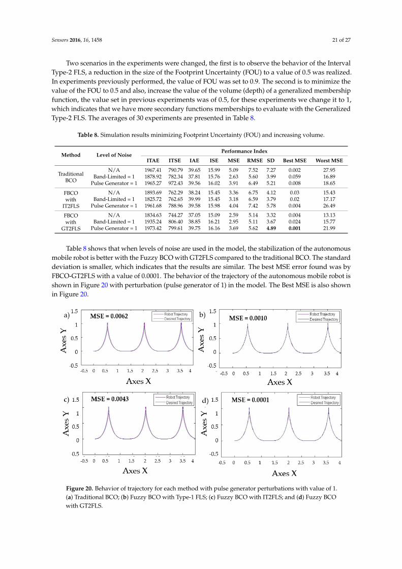
Table 8 shows that when levels of noise are used in the model, the stabilization of the autonomousmobile robot is better with the Fuzzy BCO with GT2FLS compared to the traditional BCO. The standarddeviation is smaller, which indicates that the results are similar. The best MSE error found was byFBCO-GT2FLS with a value of 0.0001. The behavior of the trajectory of the autonomous mobile robot isshown in Figure 20 with perturbation (pulse generator of 1) in the model. The Best MSE is also shownin Figure 20.

Sensors 2016, 16, 1458 22 of 28

Two scenarios in the experiments were changed, the first is to observe the behavior of the Interval Type-2 FLS, a reduction in the size of the Footprint Uncertainty (FOU) to a value of 0.5 was realized. In experiments previously performed, the value of FOU was set to 0.9. The second is to minimize the value of the FOU to 0.5 and also, increase the value of the volume (depth) of a generalized membership function, the value set in previous experiments was of 0.5, for these experiments we change it to 1, which indicates that we have more secondary functions memberships to evaluate with the Generalized Type-2 FLS. The averages of 30 experiments are presented in Table 8.

Table 8. Simulation results minimizing Footprint Uncertainty (FOU) and increasing volume.

Method Level of Noise Performance Index

ITAE ITSE IAE ISE MSE RMSE SD Best MSE

Worst MSE

Traditional BCO

N/A 1967.41 790.79 39.65 15.99 5.09 7.52 7.27 0.002 27.95 Band-Limited = 1 1878.92 782.34 37.81 15.76 2.63 5.60 3.99 0.059 16.89

Pulse Generator = 1 1965.27 972.43 39.56 16.02 3.91 6.49 5.21 0.008 18.65

FBCO with IT2FLS

N/A 1893.69 762.29 38.24 15.45 3.36 6.75 4.12 0.03 15.43 Band-Limited = 1 1825.72 762.65 39.99 15.45 3.18 6.59 3.79 0.02 17.17

Pulse Generator = 1 1961.68 788.96 39.58 15.98 4.04 7.42 5.78 0.004 26.49

FBCO with GT2FLS

N/A 1834.63 744.27 37.05 15.09 2.59 5.14 3.32 0.004 13.13 Band-Limited = 1 1935.24 806.40 38.85 16.21 2.95 5.11 3.67 0.024 15.77

Pulse Generator = 1 1973.42 799.61 39.75 16.16 3.69 5.62 4.89 0.001 21.99

Table 8 shows that when levels of noise are used in the model, the stabilization of the autonomous mobile robot is better with the Fuzzy BCO with GT2FLS compared to the traditional BCO. The standard deviation is smaller, which indicates that the results are similar. The best MSE error found was by FBCO-GT2FLS with a value of 0.0001. The behavior of the trajectory of the autonomous mobile robot is shown in Figure 20 with perturbation (pulse generator of 1) in the model. The Best MSE is also shown in Figure 20.

Figure 20. Behavior of trajectory for each method with pulse generator perturbations with value of 1. (a) Traditional BCO; (b) Fuzzy BCO with Type-1 FLS; (c) Fuzzy BCO with IT2FLS; and (d) Fuzzy BCO with GT2FLS.

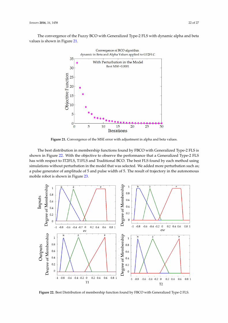
The convergence of the Fuzzy BCO with Generalized Type-2 FLS with dynamic alpha and beta values is shown in Figure 21.

Figure 20. Behavior of trajectory for each method with pulse generator perturbations with value of 1.(a) Traditional BCO; (b) Fuzzy BCO with Type-1 FLS; (c) Fuzzy BCO with IT2FLS; and (d) Fuzzy BCOwith GT2FLS.

Sensors 2016, 16, 1458 22 of 27

The convergence of the Fuzzy BCO with Generalized Type-2 FLS with dynamic alpha and betavalues is shown in Figure 21.Sensors 2016, 16, 1458 23 of 28

Figure 21. Convergence of the MSE error with adjustment in alpha and beta values.

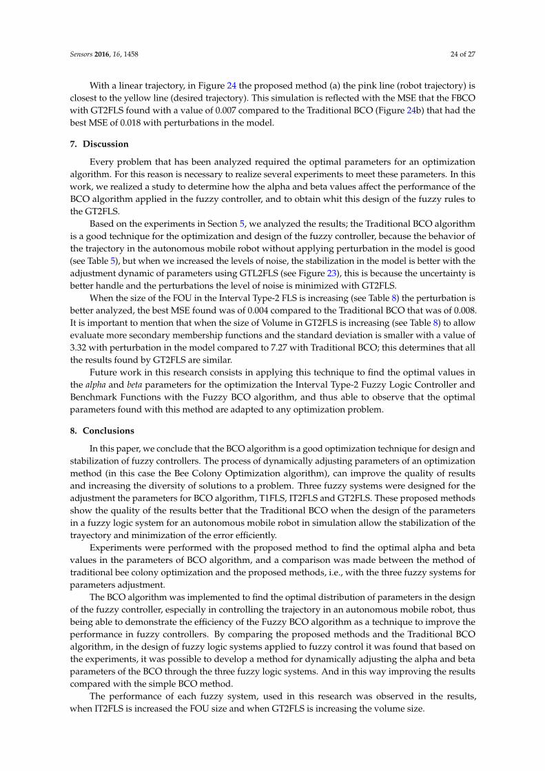
The best distribution in membership functions found by FBCO with Generalized Type-2 FLS is shown in Figure 22. With the objective to observe the performance that a Generalized Type-2 FLS has with respect to IT2FLS, T1FLS and Traditional BCO. The best FLS found by each method using simulations without perturbation in the model that was selected. We added more perturbation such as; a pulse generator of amplitude of 5 and pulse width of 5. The result of trajectory in the autonomous mobile robot is shown in Figure 23.

Figure 22. Best Distribution of membership function found by FBCO with Generalized Type-2 FLS.


The best distribution in membership functions found by FBCO with Generalized Type-2 FLS isshown in Figure 22. With the objective to observe the performance that a Generalized Type-2 FLShas with respect to IT2FLS, T1FLS and Traditional BCO. The best FLS found by each method usingsimulations without perturbation in the model that was selected. We added more perturbation such as;a pulse generator of amplitude of 5 and pulse width of 5. The result of trajectory in the autonomousmobile robot is shown in Figure 23.

Sensors 2016, 16, 1458 23 of 28


The best distribution in membership functions found by FBCO with Generalized Type-2 FLS is shown in Figure 22. With the objective to observe the performance that a Generalized Type-2 FLS has with respect to IT2FLS, T1FLS and Traditional BCO. The best FLS found by each method using simulations without perturbation in the model that was selected. We added more perturbation such as; a pulse generator of amplitude of 5 and pulse width of 5. The result of trajectory in the autonomous mobile robot is shown in Figure 23.

Figure 22. Best Distribution of membership function found by FBCO with Generalized Type-2 FLS. Figure 22. Best Distribution of membership function found by FBCO with Generalized Type-2 FLS.


Figure 23. Behavior of trajectory for each method applying perturbation in the model. (a) Traditional BCO; (b) Fuzzy BCO with Type-1 FLS; (c) Fuzzy BCO with IT2FLS; and (d) Fuzzy BCO with GT2FLS.

To observe the efficiency of proposed method, a different trajectory is shown in Figure 24, where we have shown the best experiment with FBCO with GT2FLS and the best experiment of the Traditional BCO used the perturbation pulse generator with value of 0.5 (see Table 7).

Figure 24. Behavior of the second trajectory for the proposed method applying perturbation in the model. (a) FBCO with GT2FLS (b) Traditional BCO algorithm.

Figure 23. Behavior of trajectory for each method applying perturbation in the model. (a) TraditionalBCO; (b) Fuzzy BCO with Type-1 FLS; (c) Fuzzy BCO with IT2FLS; and (d) Fuzzy BCO with GT2FLS.

To observe the efficiency of proposed method, a different trajectory is shown in Figure 24,where we have shown the best experiment with FBCO with GT2FLS and the best experiment ofthe Traditional BCO used the perturbation pulse generator with value of 0.5 (see Table 7).

Sensors 2016, 16, 1458 24 of 28

Figure 23. Behavior of trajectory for each method applying perturbation in the model. (a) Traditional BCO; (b) Fuzzy BCO with Type-1 FLS; (c) Fuzzy BCO with IT2FLS; and (d) Fuzzy BCO with GT2FLS.

To observe the efficiency of proposed method, a different trajectory is shown in Figure 24, where we have shown the best experiment with FBCO with GT2FLS and the best experiment of the Traditional BCO used the perturbation pulse generator with value of 0.5 (see Table 7).

Figure 24. Behavior of the second trajectory for the proposed method applying perturbation in the model. (a) FBCO with GT2FLS (b) Traditional BCO algorithm.

Figure 24. Behavior of the second trajectory for the proposed method applying perturbation in themodel. (a) FBCO with GT2FLS (b) Traditional BCO algorithm.

Sensors 2016, 16, 1458 24 of 27

With a linear trajectory, in Figure 24 the proposed method (a) the pink line (robot trajectory) isclosest to the yellow line (desired trajectory). This simulation is reflected with the MSE that the FBCOwith GT2FLS found with a value of 0.007 compared to the Traditional BCO (Figure 24b) that had thebest MSE of 0.018 with perturbations in the model.

7. Discussion

Every problem that has been analyzed required the optimal parameters for an optimizationalgorithm. For this reason is necessary to realize several experiments to meet these parameters. In thiswork, we realized a study to determine how the alpha and beta values affect the performance of theBCO algorithm applied in the fuzzy controller, and to obtain whit this design of the fuzzy rules tothe GT2FLS.

Based on the experiments in Section 5, we analyzed the results; the Traditional BCO algorithmis a good technique for the optimization and design of the fuzzy controller, because the behavior ofthe trajectory in the autonomous mobile robot without applying perturbation in the model is good(see Table 5), but when we increased the levels of noise, the stabilization in the model is better with theadjustment dynamic of parameters using GTL2FLS (see Figure 23), this is because the uncertainty isbetter handle and the perturbations the level of noise is minimized with GT2FLS.

When the size of the FOU in the Interval Type-2 FLS is increasing (see Table 8) the perturbation isbetter analyzed, the best MSE found was of 0.004 compared to the Traditional BCO that was of 0.008.It is important to mention that when the size of Volume in GT2FLS is increasing (see Table 8) to allowevaluate more secondary membership functions and the standard deviation is smaller with a value of3.32 with perturbation in the model compared to 7.27 with Traditional BCO; this determines that allthe results found by GT2FLS are similar.

Future work in this research consists in applying this technique to find the optimal values inthe alpha and beta parameters for the optimization the Interval Type-2 Fuzzy Logic Controller andBenchmark Functions with the Fuzzy BCO algorithm, and thus able to observe that the optimalparameters found with this method are adapted to any optimization problem.

8. Conclusions

In this paper, we conclude that the BCO algorithm is a good optimization technique for design andstabilization of fuzzy controllers. The process of dynamically adjusting parameters of an optimizationmethod (in this case the Bee Colony Optimization algorithm), can improve the quality of resultsand increasing the diversity of solutions to a problem. Three fuzzy systems were designed for theadjustment the parameters for BCO algorithm, T1FLS, IT2FLS and GT2FLS. These proposed methodsshow the quality of the results better that the Traditional BCO when the design of the parametersin a fuzzy logic system for an autonomous mobile robot in simulation allow the stabilization of thetrayectory and minimization of the error efficiently.

Experiments were performed with the proposed method to find the optimal alpha and betavalues in the parameters of BCO algorithm, and a comparison was made between the method oftraditional bee colony optimization and the proposed methods, i.e., with the three fuzzy systems forparameters adjustment.

The BCO algorithm was implemented to find the optimal distribution of parameters in the designof the fuzzy controller, especially in controlling the trajectory in an autonomous mobile robot, thusbeing able to demonstrate the efficiency of the Fuzzy BCO algorithm as a technique to improve theperformance in fuzzy controllers. By comparing the proposed methods and the Traditional BCOalgorithm, in the design of fuzzy logic systems applied to fuzzy control it was found that based onthe experiments, it was possible to develop a method for dynamically adjusting the alpha and betaparameters of the BCO through the three fuzzy logic systems. And in this way improving the resultscompared with the simple BCO method.

The performance of each fuzzy system, used in this research was observed in the results,when IT2FLS is increased the FOU size and when GT2FLS is increasing the volume size.

Sensors 2016, 16, 1458 25 of 27

Acknowledgments: We thank the MyDCI program of ITT University, the Division of Graduate Studies andResearch of Tijuana Institute of Technology and the financial support provided by CONACYT contract grantNumber: 261565.

Author Contributions: Juan Ramon Castro, Olivia Mendoza and Antonio Rodriguez Diaz designed the toolbox ofthe Generalized Type-2 Fuzzy Logic Systems; Oscar Castillo and Patricia Melin contributed to the discussion andanalysis of the results; Leticia Amador Angulo analyzed of the model in as autonomous mobile robot, contributedof the simulations and wrote the paper.

Conflicts of Interest: The authors declare no conflict of interest.

Abbreviations

BCO Bee Colony OptimizationT1FLS Type-1 Fuzzy Logic SystemIT2FLS Interval Type-2 Fuzzy Logic SystemGT2FLS Generalized Type-2 Fuzzy Logic SystemFLC Fuzzy Logic Controller.MSE Mean Square ErrorRMSE Root Mean Square ErrorITAE Integrated Time Absolute ErrorITSE Integrated Time Square ErrorIAE Integrated Absolute ErrorISE Integrated Square ErrorSD Standard Desviation

References

1. Zadeh, L.A. Fuzzy Sets. Inf. Control 1965, 8, 338–353. [CrossRef]2. Banklouti, N.; John, R.; Alimi, A.M. Interval type-2 fuzzy logic control of mobile robot. Inf. Learn. Syst. Appl.

2012, 4, 291–302.3. Sánchez, M.A.; Castillo, O.; Castro, J.R. Generalized type-2 fuzzy systems for controlling a mobile robot

and a performance comparison with interval type-2 and type-1 fuzzy systems. Expert Syst. Appl. 2015, 42,5904–5914. [CrossRef]

4. Martinez, R.; Castillo, O.; Aguilar, L. Optimization of interval type-2 fuzzy logic controllers for a perturbedautonomous wheeled mobile robot using genetic algorithms. Inf. Sci. 2009, 179, 2158–2174. [CrossRef]

5. Grelle, C.; Ippolito, L.; Loia, V.; Siano, P. Agent-based architecture for designing hybrid control systems.Inf. Sci. 2006, 176, 1103–1130. [CrossRef]

6. Zi, B.; Zhu, Z.C.; Du, J.L. Analysis and control of the cable-supporting system including actuator dynamics.Control Eng. Pract. 2011, 19, 491–501. [CrossRef]

7. Zi, B.; Ding, H.; Cao, J.; Zhu, Z.; Kecskeméthy, A. Integrated mechanism design and control for completelyrestrained hybrid-driven based cable parallel manipulators. J. Intell. Robot. Syst. 2014, 74, 643–661. [CrossRef]

8. Gao, Z.; Zhang, D. Performance analysis, mapping, and multiobjective optimization of a hybrid roboticmachine tool. IEEE Trans. Ind. Electron. 2015, 62, 423–433. [CrossRef]

9. Rachman, E.; Jaam, J.M.; Hasnah, A.M. Non-linear simulation of controller for longitudinal controlaugmentation system of F-16 using numerical approach. Inf. Sci. 2004, 164, 47–60. [CrossRef]

10. Hagras, H.; Sobh, T. Intelligent learning and control of autonomous robotic agents operating in unstructuredenvironments. Inf. Sci. 2002, 145, 1–12. [CrossRef]

11. Zadeh, L.A. Toward a theory of fuzzy information granulation and its centrality in human reasoning andfuzzy logic. Fuzzy Sets Syst. 1997, 90, 111–127. [CrossRef]

12. Mendel, J.M.; Mouzouris, G.C. Type-2 fuzzy logic system. IEEE Trans. Fuzzy Syst. 1999, 7, 642–658.13. Mendel, J.M.; John, R.I.B. Type-2 fuzzy sets made simple. IEEE Trans. Fuzzy Syst. 2002, 10, 117–127.

[CrossRef]14. Linda, O.; Manic, M. Monotone centroid flow algorithm for type reduction on general type-2 fuzzy sets.

IEEE Trans. Fuzzy Syst. 2012, 20, 805–819. [CrossRef]15. Mo, H.; Wang, F.-Y.; Zhou, M.; Li, R.; Xiao, Z. Footprint of uncertainty for type-2 fuzzy sets. Inf. Sci. 2014,

272, 96–110. [CrossRef]

http://dx.doi.org/10.1016/S0019-9958(65)90241-X

http://dx.doi.org/10.1016/j.eswa.2015.03.024

http://dx.doi.org/10.1016/j.ins.2008.12.028


http://dx.doi.org/10.1016/j.conengprac.2011.02.001

http://dx.doi.org/10.1007/s10846-013-9848-0

http://dx.doi.org/10.1109/TIE.2014.2327008


http://dx.doi.org/10.1016/S0020-0255(02)00221-9

http://dx.doi.org/10.1016/S0165-0114(97)00077-8

http://dx.doi.org/10.1109/91.995115

http://dx.doi.org/10.1109/TFUZZ.2012.2185502


Sensors 2016, 16, 1458 26 of 27

16. Yeh, C.-Y.; Jeng, W.-H.R.; Lee, S.-J. An enhanced type-reduction algorithm for type-2 fuzzy sets. IEEE Trans.Fuzzy Syst. 2011, 19, 227–240. [CrossRef]

17. Zhao, L.; Li, Y.; Li, Y. Computing with words for discrete general type-2 fuzzy sets based on α plane.In Proceedings of the 2013 IEEE International Conference on Vehicular Electronics and Safety, Dongguan,China, 28–30 July 2013; pp. 268–272.

18. Sanchez, M.A.; Castro, J.R.; Castillo, O. Formation of general type-2 Gaussian membership functions basedon the information granule numerical evidence. In Proceedings of the 2013 IEEE Workshop on HybridIntelligent Models and Applications (HIMA), Singapore, 16–19 April 2013; pp. 1–6.

19. Mamdani, E.H. Applications of fuzzy algorithms for simple dynamic plant. Proc. IEEE 1974, v121, 1585–1588.[CrossRef]

20. Zadeh, L.A. The concept of a lingüistic variable and its application to approximate reasoning, Part I. Inf. Sci.1975, 8, 199–249. [CrossRef]

21. Zadeh, L.A. The concept of a lingüistic variable and its application to approximate reasoning, Part II. Inf. Sci.1975, 8, 301–357. [CrossRef]

22. Angelov, P.P.; Buswell, R.A. Automatic generation of fuzzy rule-based models from data by geneticalgorithms. Inf. Sci. 2003, 150, 17–31. [CrossRef]

23. Sanchez, E.N.; Becerra, H.M.; Velez, C.M. Combining fuzzy, PID and regulation control for an autonomousmini-helicopter. Inf. Sci. 2007, 177, 1999–2022. [CrossRef]

24. García-Nieto, S.; Salcedo, J.; Martínez, M.; Laurí, D. Air management in a diesel engine using fuzzy controltechniques. Inf. Sci. 2009, 179, 3392–3409. [CrossRef]

25. Boulkroune, A.; M’Saad, M.; Chekireb, H. Design of a fuzzy adaptive controller for MIMO nonlineartime-delay systems with unknown actuator nonlinearities and unknown control direction. Inf. Sci. 2010, 180,5041–5059. [CrossRef]

26. Zaheer, S.A.; Choi, S.H.; Jung, C.Y.; Kim, J.H. A modular implementation scheme for nonsingleton type-2fuzzy logic systems with input uncertainties. IEEE/ASME Trans. Mechatron. 2015, 20, 3182–3193. [CrossRef]

27. Xie, X.P.; Yue, D.; Hu, S.L. Fuzzy control design of nonlinear systems under unreliable communication links:A systematic homogenous polynomial approach. Inf. Sci. 2016. in press. [CrossRef]

28. Corne, D.; Dorigo, M.; Glover, F. New Ideas in Optimization; McGraw-Hill: New York, NY, USA, 1999.29. Arabshahi, P.; Choi, J.J.; Marks, R.J.; Caudell, T.P. Fuzzy parameter adaptation in optimization: Some neural

net training examples. IEEE Comput. Sci. Eng. 1996, 3, 57–65. [CrossRef]30. Shi, Y.; Eberhart, R.C. Fuzzy adaptive particle swarm optimization. In Proceedings of the 2001 Congress on

Evolutionary Computation, Seoul, Korea, 26–30 May 2001; pp. 101–106.31. Chatterjee, A.; Siarry, P. Nonlinear inertia weight variation for dynamic adaptation in particle swarm

optimization. Comput. Oper. Res. 2006, 33, 859–871. [CrossRef]32. Melin, P.; Olivas, F.; Castillo, O.; Valdez, F.; Soria, J.; Valdez, M. Optimal design of fuzzy classification

systems using PSO with dynamic parameter adaptation through fuzzy logic. Expert Syst. Appl. 2013, 40,1–12. [CrossRef]

33. Ochoa, P.; Castillo, O. Differential evolution with dynamic adaptation of parameters of the optimization ofFuzzy Controller. In Recent Advance of Hybrid Approach for Designing Intelligent Systems; Springer InternationalPublishing: Tijuana, Mexico, 2014; pp. 275–288.

34. Lucic, P.; Teodorovic, D. Vehicle routing problem with uncertain demand at nodes: The bee system andfuzzy logic approach. In Fuzzy Sets Based Heuristics for Optimization; Verdegay, J.L., Ed.; Springer-Verlag:Heidelberg, Germany; Berlin, Germany, 2003; pp. 67–82.

35. Teodorovic, D. Transport modeling by multi-agent systems: A swarm intelligence approach.Transp. Plan. Technol. 2003, 26, 289–312. [CrossRef]

36. Teodorovic, D. Swarm intelligence systems for transportation engineering: Principles and applications.Transp. Res. Part C Emerg. Technol. 2008, 16, 651–782. [CrossRef]

37. Chong, C.; Low, M.; Sivakumar, A.K.; Gay, K.L. A bee colony optimization algorithm to job shop scheduling.In Proceedings of the 2006 Winter Simulation Conference, Monterey, CA, USA, 3–6 December 2006.

38. Wong, L.P.; Chong, C.S. An efficient bee colony optimization algorithm for traveling salesman problemusing frequency-based pruning. In Proceedings of the 7th International Conference on Industrial Informatics(INDIN 2009), Cardiff, UK, 24–26 June 2009; pp. 775–782.


http://dx.doi.org/10.1049/piee.1974.0328

http://dx.doi.org/10.1016/0020-0255(75)90036-5

http://dx.doi.org/10.1016/0020-0255(75)90046-8

http://dx.doi.org/10.1016/S0020-0255(02)00367-5




http://dx.doi.org/10.1109/TMECH.2015.2411853


http://dx.doi.org/10.1109/99.486761

http://dx.doi.org/10.1016/j.cor.2004.08.012

http://dx.doi.org/10.1016/j.eswa.2012.12.033

http://dx.doi.org/10.1080/0308106032000154593

http://dx.doi.org/10.1016/j.trc.2008.03.002

Sensors 2016, 16, 1458 27 of 27

39. Chaiyatham, T.; Ngamroo, I. A bee colony optimization based-fuzzy logic-PID control design of electrolyzerfor microgrid stabilization. Int. J. Innov. Comput. Inf. Control 2012, 8, 6049–6066.

40. Tiacharoen, S.; Chatchanayuenyong, T. Design and development of an intelligent control by using bee colonyoptimization technique. Am. J. Appl. Sci. 2012, 9, 1464–1471.

41. Amador-Angulo, L.; Castillo, O. Comparison of the optimal design of fuzzy controllers for the water tankusing ant colony optimization. In Recent Advances on Hybrid Approaches for Designing Intelligent Systems;Springer: Tijuana, Mexico, 2014.

42. Amador-Angulo, L.; Castillo, O. A new algorithm based in the smart behavior of the bees for the designof mamdani-style fuzzy controllers using complex non-linear plants. In Design of Intelligent Systems Basedon Fuzzy Logic, Neural Network and Nature-Inspired Optimization; Springer International Publishing: Tijuana,Mexico, 2015; pp. 617–637.

43. Mendel, J.M. A quantitative comparison of interval type-2 and type1fuzzy logic systems: First results.In Proceedings of the IEEE International Conference on Fuzzy Systems (FUZZ), Barcelona, Spain,18–23 July 2010; pp. 1–8.

44. Karnik, N.N.; Mendel, J.; Liang, Q. Type-2 fuzzy logic systems. IEEE Trans. Fuzzy Syst. 1999, 7, 643–658.[CrossRef]

45. Karnik, N.N.; Mendel, J.M. Operations on type-2 fuzzy sets. Int. J. Fuzzy Sets Syst. 2001, 122, 327–348.[CrossRef]

46. Mendel, J.M. Uncertain Rule-Based Fuzzy Logic System: Introduction and New Directions; Practice Hall: New York,NY, USA, 2001.

47. Mendel, J.M. On km algorithms for solving type-2 fuzzy set problems. IEEE Trans. Fuzzy Syst. 2013, 21,426–446. [CrossRef]

48. Mendel, J.; Hani, H.; Tan, W.-W.; Melek, W.W.; Ying, H. Introduction to Type-2 Fuzzy Logic Control;John Wiley & Sons, Inc.: Hoboken, NJ, USA, 2014.

49. Mendel, J.M. Enhanced karnik—Mendel algorithms. IEEE Trans. Fuzzy Syst. 2009, 17, 923–934.50. Chen, S.; Chang, Y.; Pan, J. Fuzzy Rules Interpolation for Sparse Fuzzy Rule-Based Systems Based on Interval

Type-2 Gaussian Fuzzy Sets and Genetic Algorithms. IEEE Trans. Fuzzy Syst. 2013, 21, 412–425. [CrossRef]51. Wagner, C.; Miller, S.; Garibaldi, J.; Anderson, D.; Havens, T. From interval-valued data to general type-2

fuzzy sets. IEEE Trans. Fuzzy Syst. 2105, 23, 248–269. [CrossRef]52. Naim, S.; Hagras, H. A general type-2 fuzzy logic based approach for Multi-Criteria Group Decision Marking.

In Proceedings of the 2013 IEEE International Conference on Fuzzy System (FUZZ-IEEE), Hyderabad, India,7–10 July 2103; pp. 1–8.

53. Hagras, H.A. Type-2 FLC: A new Generalization of Fuzzy Controllers. IEEE Comput. Intell. Mag. 2007, 2,30–43. [CrossRef]

54. Melin, P.; Gonzalez, C.; Castro, J.R.; Castillo, O. Edge detection method for image processing on generalizedtype-2 fuzzy logic. IEEE Trans. Fuzzy Syst. 2014, 22, 1515–1525. [CrossRef]

55. Mendel, J.M.; Liu, F.; Zhai, D. α-Plane Representation for Type-2 Fuzzy Sets: Theory and applications.IEEE Trans. Fuzzy Syst. 2009, 17, 1189–1207. [CrossRef]

56. Mendel, J.M. Comments on alpha-plane representation for type-2 fuzzy sets: Theory and applications.IEEE Trans. Fuzzy Syst. 2010, 18, 229–230. [CrossRef]

57. Hao, M.; Mendel, J.M. Similarity measures for general type-2 fuzzy sets based on the -plane representation.Inf. Sci. 2014, 277, 197–215. [CrossRef]

58. Doostparast Torshizi, A.; Zarandi, M.H.F. Hierarchical collapsing method for direct defuzzification of generaltype-2 fuzzy sets. Inf. Sci. 2014, 277, 842–861. [CrossRef]

59. Castillo, O.; Amador-Angulo, L.; Castro, J.R.; Garcia-Valdez, M. A comparative study of type-1 fuzzy logicsystems, interval type-2 fuzzy logic systems and generalized type-2 fuzzy logic systems in control problems.Inf. Sci. 2016, 354, 257–274. [CrossRef]

60. Biesmeijer, J.C.; Seeley, T.D. The use of waggle dance information by honey bees throughout their foragingcareers. Behav. Ecol. Sociobiol. 2005, 59, 133–142. [CrossRef]

© 2016 by the authors; licensee MDPI, Basel, Switzerland. This article is an open accessarticle distributed under the terms and conditions of the Creative Commons Attribution(CC-BY) license (http://creativecommons.org/licenses/by/4.0/).

http://dx.doi.org/10.1109/91.811231

http://dx.doi.org/10.1016/S0165-0114(00)00079-8




http://dx.doi.org/10.1109/MCI.2007.357192







http://dx.doi.org/10.1007/s00265-005-0019-6

http://creativecommons.org/

http://creativecommons.org/licenses/by/4.0/.

Fuzzy Sets in Dynamic Adaptation of Parameters of a Bee ...

Documents

Transcript of Fuzzy Sets in Dynamic Adaptation of Parameters of a Bee ...