Fusuma: Double-Ended Threaded Compaction(Full Version)

Fusuma: Double-Ended Threaded Compaction(Full Version)

Hiro OnozawaGraduate School of

Informatics and EngineeringThe University of

Electro-CommunicationsTokyo, Japan

[email protected]

Tomoharu UgawaGraduate School of

Information Science and TechnologyThe University of Tokyo

Tokyo, [email protected]

Hideya IwasakiGraduate School of

Informatics and EngineeringThe University of

Electro-CommunicationsTokyo, Japan

[email protected]

AbstractJonkers’s threaded compaction is attractive in the contextof memory-constrained embedded systems because of itsspace efficiency. However, it cannot be applied to a heapwhere ordinary objects and meta-objects are intermingledfor the following reason. It requires the object layout informa-tion, which is often stored in meta-objects, to update pointerfields inside objects correctly. Because Jonkers’s threadedcompaction reverses pointer directions during garbage col-lection (GC), it cannot follow the pointers to obtain the ob-ject layout. This paper proposes Fusuma, a double-endedthreaded compaction that allows ordinary objects and meta-objects to be allocated in the same heap. Its key idea is tosegregate ordinary objects at one end of the monolithic heapand meta-objects at the other to make it possible to sepa-rate the phases of threading pointers in ordinary objectsand meta-objects. Much like Jonkers’s threaded compaction,Fusuma does not require any additional space for each object.We implemented it in eJSVM, a JavaScript virtual machinefor embedded systems, and compared its performance witheJSVM using mark-sweep GC. As a result, compaction en-abled an IoT-oriented benchmark program to run in a 28-KiBheap, which is 20 KiB smaller than mark-sweep GC. We alsoconfirmed that the GC overhead of Fusuma was less than2.50× that of mark-sweep GC.

Keywords: garbage collection, JavaScript, compaction, meta-object, embedded systems

1 IntroductioneJS [19] is a JavaScript processing system for embedded sys-tems such as IoT devices, where approximately 100 KB ofmemory is available for the heap. It generates a customized

ISMM ’21, June 22, 2021, Virtual, Canada© 2021 Association for Computing Machinery.This is the author’s version of the work. It is posted here for your personaluse. Not for redistribution. The definitive Version of Record was published inProceedings of the 2021 ACM SIGPLAN International Symposium on MemoryManagement (ISMM ’21), June 22, 2021, Virtual, Canada, https://doi.org/10.1145/3459898.3463903.

JavaScript virtual machine (VM), eJSVM, for a specific appli-cation based on a VM configuration given by the applicationdeveloper.

The standard eJSVM configuration uses mark-sweep gar-bage collection (GC). Because mark-sweep GC does not moveobjects, the VM may suffer from fragmentation; even if thetotal free space in the heap is sufficient, the program may failto allocate a contiguous area for an object. One way to solvethis fragmentation problem is to use compaction. Jonkers’sthreaded compaction [12] is a memory-efficient compactionalgorithm. Unlike other sliding compaction methods, it doesnot use extra words in the object header or in any side tables.For example, Lisp2 [14] compaction uses one extra word fora forwarding pointer, and the Compressor [13] uses a sidetable. Because space overhead of a few kilobytes is seriousin a 100-KB heap, this attribute is attractive.The current eJSVM records the layout information of

JavaScript first class objects, or ordinary objects, in meta-objects called hidden classes [4] to execute JavaScript pro-grams efficiently. Because a hidden class is made up of mul-tiple meta-objects connected by pointers, the pointers insidemeta-objects must be followed to obtain the object layout.Such meta-objects are allocated in the same heap as ordinaryobjects and are subject to GC.

Jonkers’s threaded compaction scans the heap after mark-ing live objects to thread all pointers in the object. The layoutof each object must be known during the threading pro-cess. However, because the threading operation reverses thepointer direction, threaded pointers cannot be followed untilthey are unthreaded. Because of this, if ordinary objects andmeta-objects are allocated in the same heap, the object layoutcannot be obtained.One possible way to cope with this problem is to use a

dedicated space for meta-objects that is separate from thespace for ordinary objects. However, separate spaces mightinduce space-level fragmentation, where one space becomesfull while the other has an excess of free space. This mightbe fatal in memory-constrained environments.

https://doi.org/10.1145/3459898.3463903

https://doi.org/10.1145/3459898.3463903

ISMM ’21, June 22, 2021, Virtual, Canada Hiro Onozawa, Tomoharu Ugawa, and Hideya Iwasaki

This paper proposes double-ended threaded compactionnamed Fusuma1 to resolve this problem. Fusuma distin-guishes between ordinary objects and meta-objects whenallocating them: ordinary objects are allocated from one endof the monolithic heap and the meta-objects that make upthe hidden classes from the other end. During compaction,pointers in ordinary objects are threaded first, and then themeta-objects, which have a statically determined layout, arethreaded. By threading in this order, GC can follow pointersin meta-objects to obtain the layout of ordinary objects be-cause the meta-objects have not yet been threaded duringordinary object processing. Finally, live ordinary objects andmeta-objects are slid toward the left and the right respec-tively. As in Jonkers’s algorithm, Fusuma does not requireany additional space.We implemented Fusuma in eJSVM and evaluated its

performance using several benchmark programs. Compact-ing the heap enabled an IoT-oriented benchmark programto run in a 28-KiB heap, which is 20 KiB smaller than formark-sweep GC. We also confirmed that the GC overheadof Fusuma was less than 2.50× that of mark-sweep GC.The problem addressed in this paper is not specific to

eJSVM. For example, in the V8 JavaScript Engine2, the GCneeds to follow pointers in hidden classes to determinewhether each property is a pointer or an unboxed value[7]. Implementing Jonkers’s compaction in such a systeminvolves the same problem as eJSVM, which can be solved byFusuma. Furthermore, other in-place sliding compactions [10,14] share essentially the same problem addressed in thispaper. The central idea of Fusuma, sliding objects in twodirections, can be applied to them to solve the problem, asdiscussed in Section 7.This paper first describes eJS in Section 2, followed by

Jonkers’s compaction algorithm and its problems in Section3. Next, Section 4 proposes Fusuma, a double-ended threadedcompaction algorithm, and Section 5 describes its implemen-tation issues in eJSVM. Section 6 evaluates the performanceof Fusuma implemented in Section 5 by means of experi-ments. Section 7 introduces related work, and finally, Section8 concludes the paper.

2 eJS2.1 OvervieweJS (embedded JavaScript) [19] is a JavaScript processingsystem for embedded systems such as IoT devices, whereapproximately 100 KB of memory is available for the heap. Itreduces the workload of program developers, improves appli-cation development efficiency, and facilitates prototyping byenabling development on embedded systems in JavaScript.

1Fusuma is a bi-part sliding partition in a traditional Japanese room.2https://v8.dev/

(a) Immediate value.

(b) Pointer.

Figure 1. JSValue in eJSVM.

The eJS framework can automatically generate eJSVM,which is a JavaScript VM customized for a specific appli-cation program to run on a specific embedded system. Forexample, the developer can specify datatypes to be distin-guished with pointer tagging. eJS generates efficient typedispatching code in eJSVM based on the developer’s specifi-cation. The eJS framework supports both 32-bit and 64-bitprocessors. Currently, eJSVM runs with an interpreter with-out just-in-time (JIT) compilation.

2.2 Object LayoutIn eJSVM, every first-class value in JavaScript is representedby a single-word JSValue type. Its structure is presented inFigure 1. A value of JSValue has type information calleda PTAG (pointer tag) and either an immediate value or anobject address in a single word. When a value of the JSValuetype is an integer, a boolean, or a special value such asundefined, an immediate value is stored. When it repre-sents an ordinary object such as an Object or an Array,the address of the object is used. Because every object isword-aligned in the heap area, the lower two or three bits(depending on word size) of an object address are alwayszero. These bits are used for PTAG. The developer can specifya few datatypes that have separate PTAG values to examinethe types quickly. Other datatypes share the same PTAG val-ues and can be distinguished by the type information calledthe HTAG (header tag) in the object header described below.An ordinary object consists of four elements: an object

header, a pointer to a hidden class, an internal property area,and a pointer to an external property array, if any. The objectheader is a single word containing the object’s size, type(HTAG), and the mark bit used in GC. The hidden classrecords the object layout. An object reference points to thenext word to the object header, as presented in Figure 1 (b).

Invisible properties from the JavaScript program that areinherently possessed by an ordinary object when it is cre-ated, such as the pointer to the code of a built-in function,are called special properties. Associated values with specialproperties are stored as non-JSValues at the beginning ofthe internal property area, with some exceptions, which GCtakes care of in an ad-hoc way.

https://v8.dev/

Fusuma: Double-Ended Threaded Compaction ISMM ’21, June 22, 2021, Virtual, Canada

var A = {}; // Step 1A.a = 100 // Step 2A.b = "Hello" // Step 3var B = {}; // Step 4B.a = 200 // Step 5

(a) JavaScript code.(b) Step 1.

(c) Step 2.

(d) Step 3. (e) Step 4. (f) Step 5.

Figure 2. Example of growing hidden classes.

As in other JavaScript VMs [6], properties that are likelyto be added to an ordinary object in the future are reservedin advance as internal properties when the object is allocated.They are determined based on the execution history of theprogram up to the point where the object is allocated. Otherproperties that are attached dynamically during programexecution are stored in the external property array.

2.3 Hidden ClassesJavaScript can dynamically add and remove the properties ofobjects. A naive implementation for such dynamic additionand deletion of properties uses an array or hash table of key-value pairs, where the key is a property name, and the valueis its associated value. However, this naive implementationis not efficient.

A common technique to deal efficiently with JavaScript’sdynamic behavior is to use hidden classes [4]. When usinghidden classes, each object manages only its property valuesin an array, which is called the property array. In addition tothis, each object has a pointer to its hidden class. A hiddenclass essentially manages mappings from property names toindices in the property array. Hidden classes are immutable;they can be shared among multiple objects with the sameset of property names that have been attached in the sameorder. When a new property is added to an object, a newhidden class containing both the existing properties and thenew property is created. This new hidden class is linked bya transition edge from the previously used hidden class. Thetransition edge is followed to find the new hidden class whenthe property of the same name is added to another objectthat shares the previously used hidden class. Figure 2 showsan example of hidden classes that grow as properties areadded to objects.

Hidden classes can improve space efficiency because theinformation on where object properties are stored is sharedamong multiple objects. In addition, access to propertiescan be accelerated by using inline caching [9, 11], whichpremises hidden classes.

2.4 Implementation of Hidden Classes in eJSVMA hidden class in eJSVM consists of two kinds of meta-objects: one is the Layout, and the other includes the Prop-ertyMaps and their related objects. Each meta-object has asimilar header to that of an ordinary object.

Figure 3 shows the structure of these meta-objects. A Lay-out represents the memory layout of ordinary objects thathold it. More specifically, it represents the size of the inter-nal property area and that of the external property array. APropertyMap is essentially a table representing the mappingsfrom property names to the locations of their associated val-ues or transition edges. The second slot of the PropertyMapin Figure 3 holds the pointer to the table, which is omittedin the figure. A PropertyMap also contains the total numberof properties and the number of special properties.Each ordinary object could have a Layout and a Proper-

tyMap. Instead, eJSVM saves space by putting the pointerto the PropertyMap in the Layout. In Figure 3, Object1and Object2 have different numbers of internal properties.Therefore, their Layouts are different, but they share thesame PropertyMap.

The GC refers to these meta-objects to obtain the sizes ofthe internal property area and the external property arraystored in the Layout and to obtain the number of specialproperties, which is stored in the PropertyMap. Specifically,GC needs to follow the pointer to the PropertyMap storedin the Layout to obtain the number of special properties.


Figure 3. Structure of a hidden class in eJSVM.

There are cases where meta-objects become garbage andare reclaimed by GC in eJSVM. For example, a prototypeobject is unlikely to share its PropertyMap with other objectsbecause each prototype object is usually created only once.Therefore, PropertyMaps created during initialization of pro-totype objects are likely to be tentative. The eJSVM unlinkssuch tentative PropertyMaps from the transition edge. Thedetails of this are beyond the scope of this paper.

3 Jonkers’s Threaded Compaction3.1 OverviewThe threaded compaction algorithm by Jonkers [12] per-forms space-efficient sliding compaction. This algorithmtransforms multiple pointers to the same object into a linearlist of locations for the pointers by reversing the pointerdirection through an operation called threading. Thanks tothe threading operation, Jonkers’s algorithm does not re-quire any extra space in an object, as opposed to the Lisp2algorithm [14].Figure 4 (a)–(b) presents the relation between pointers

and objects before and after threading. After threading, theheader area of the object becomes the head of the list oflocations that pointed to the object. This list of threadedpointers is called the threaded list from the object. The endof the threaded list contains the original value in the objectheader (“X” in Figure 4). Jonkers’s algorithm must recognizethat it does not hold a threaded pointer to detect the end ofa threaded list.After determining an object’s destination, to which the

object is to be moved, the algorithm unthreads the threadedlist to update every location that pointed at the object beforethreadingwith the destination address, as presented in Figure

4 (c). The pointer locations to be updated can be found byfollowing the threaded list from the object header.

3.2 AlgorithmJonkers’s compaction algorithm consists of three phases:the mark phase, the update-forward-reference phase, andthe update-backward-reference phase. Figure 5 presents anexample of a heap when this algorithm is applied. The twopointers on the left of each sub-figure represent the roots,and the wide area on their right represents the heap. Thevalue in the header of an object, e.g., a, is used to name theobject itself, for example, “object a.”First, the mark phase marks all live objects, which are

reachable from the roots. The roots are pointers to objectsin the heap from outside. The heap after the mark phaseis presented in Figure 5 (a). In this figure, the gray color ofobjects indicates that they are alive.Next, the update-forward-reference phase updates every

pointer that points to a live object forward in the heap withthe destination address, to which the object is to be moved(Figure 5 (b)–(f)). First, this phase threads all pointers in theroots. It then scans the heap from the left to find live objectsand performs the following operations on every live object.First, it unthreads the threaded list from the object by up-dating every location in the list with its destination address.Because the heap is scanned from the left, the destinationaddress is determined by summing up the sizes of all liveobjects found so far. Next, the phase threads all pointers inthe object. The heap area after the update-forward-referencephase is presented in Figure 5 (f), where only backward ref-erences remain threaded.Finally, the update-backward-reference phase moves all

live objects while unthreading backward pointers (Figure5 (g)–(j)). As in the update-forward-reference phase, theupdate-backward-reference phase scans the heap area fromthe left and performs the following operations on every liveobject. First, it unthreads the threaded list from the objectby updating every location in the list with its destinationaddress. Then it moves the object to the destination address.The heap area after this phase is presented in Figure 5 (j),where all live objects have been slid toward the left of theheap and all pointers have been correctly updated.

3.3 ProblemDuring the mark and update-forward-reference phases, thelayout information of every object is indispensable to knowthe locations of pointer fields in the object. In eJSVM, thenumbers of internal and external properties in the Layoutand the number of special properties in the PropertyMap arenecessary. If eJSVM implements unboxing [7] in the future,information about whether each field holds a JSValue oran unboxed value will also be stored in PropertyMaps. Un-fortunately, when both meta-objects that constitute hidden


(a) Before threading. (b) After threading. (c) After unthreading.

original pointer threaded pointer unthreaded (updated) pointer

Figure 4. Threading and unthreading.

(a) M: finished (b) F: threading root pointer is done

(c) F: begin of processing object a (d) F: begin of processing object b

(e) F: begin of processing object c (f) F: finished

(g) B: begin of processing object a (h) B: begin of processing object b

(i) B: begin of processing object c (j) B: finished

original pointer threaded pointer updated pointerM: mark phase, F: update-forward-reference phase, B: update-backward-reference phase

Figure 5. Example of heap with Jonkers’s threaded compaction applied.

classes and ordinary objects are intermingled in the sameheap, the following problem might occur.

Suppose that an ordinary object, its Layout, and its Prop-ertyMap reside in the heap in the order of the Layout, theobject, and the PropertyMap, as presented in Figure 6 (a).In the update-forward-reference phase, the pointer in theLayout to the PropertyMap is threaded first (Figure 6 (b)).Then, when processing the object, it is possible to reach theLayout from the object, but the number of special propertiesin the PropertyMap is inaccessible because the pointer fromthe Layout to the PropertyMap has already been threaded.As a result, it is impossible to know the layout of the object,which prevents Jonkers’s algorithm from being applied.

4 Double-Ended Threaded CompactionThis paper proposes Fusuma, a double-ended threaded com-paction algorithm that solves the problem described in Sec-tion 3.3.Assume that the system has ordinary objects and meta-

objects and that they reside in the same monolithic heap. GCmay need to follow pointers in meta-objects to obtain thelayout information of ordinary objects. It does not matterwhether meta-objects have pointers to ordinary objects ifGC does not follow them. For example, hidden classes havepointers to string objects, which are ordinary objects, ineJSVM, but GC does not follow the pointers.


(a) Before threading.

(b) After threading pointers in Layout.original pointer threaded pointer

Figure 6. Problem in Jonkers’s algorithm.

Figure 7. Heap usage of Fusuma.

4.1 Basic IdeaFusuma has the same phases as Jonkers’s compaction.The basic idea of the proposed algorithm is that, in the

update-forward-reference phase, it processes all ordinaryobjects first, during which it refers to meta-objects for layoutinformation to determine the locations of pointer fields insideordinary objects. Afterwards, it processes meta-objects. Notethat the layout of every meta-object is statically determined.For this purpose, ordinary objects are allocated from the

left of the heap in the forward direction and meta-objectsfrom the right in the backward direction (Figure 7). The heaparea where ordinary objects are allocated is called the ordi-nary object area, and that where meta-objects are allocatedis called the meta-object area.

During the compaction, ordinary objects and meta-objectsare slid toward the left end and the right end of the heap re-spectively. Therefore, in the update-forward-reference phaseand update-backward-reference phase, ordinary objects arescanned from the left, whereas meta-objects are scannedfrom the right.

4.2 AlgorithmFigure 8 presents the pseudo code of Fusuma. In this code,metaObjectTop(to,size) returns the top address of themeta-object of which the bottom is pointed to by to, andpointerToObject(p) returns the pointer to the ordinaryobject / meta-object with a top address of p. For the caseof eJSVM, p points to the object header, and this functionreturns the address of the next word to the header. Func-tion getMetaObjectSize(b) determines the size of a meta-object from its bottom address b. As for the other helperfunctions, their names are self-explanatory. Figure 9 pro-vides an example of a heap when Fusuma is applied.

Much like Jonkers’s compaction, Fusuma consists of threephases: the mark phase, the update-forward-reference phase,and the update-backward-reference phase. The mark phaseis the same as that of Jonkers’s compaction.The update-forward-reference phase can be divided into

three steps (function updateForwardReferences()). Thefirst step (foreach loop) threads all pointers in the roots (Fig-ure 9 (a)–(b)). The second step (the first while loop) scansthe ordinary object area from the left in the forward direc-tion, as in the update-forward-reference phase of Jonkers’salgorithm (Figure 9 (b)–(c)). Finally, the third step (the sec-ond while loop) scans the meta-object area from the rightin the reverse direction (Figure 9 (c)–(e)). The processingfor each live meta-object found during the third step is thesame as for each live ordinary object in the second step; first,the algorithm unthreads the threaded list by updating everylocation in the list with the new destination address, andthen it threads every pointer in the meta-object.The update-backward-reference phase (function update

BackwardReferences()) scans (in the first while loop) theobject area in the forward direction (Figure 9 (e)–(f)), andthen scans (in the second while loop) the meta-object areain the reverse direction (Figure 9 (f)–(h)). The operation foreach ordinary object / meta-object is the same as the oper-ation performed in the update-backward-reference phasein Jonkers’s algorithm; it unthreads the threaded list andthen moves the object to its destination address. Please notethat an ordinary object is moved toward the left of the heap,whereas a meta-object is moved toward the right.

By processing all ordinary objects before threading thepointers inside meta-objects in the update-forward-referencephase, the problem described in Section 3.3 is solved.

5 Implementation5.1 Boundary TagsFusuma scans the meta-object area from right to left. Tomake this possible, Fusuma places size information not onlyin the header of every meta-object, but also in the next wordof the meta-object. This size information at the bottom of ameta-object is called the boundary tag. Although no left-to-right iteration is performed on the meta-objects, the objectheader, including size and type, is still needed at the left ofeach meta-object to make it possible to obtain its type in thesame manner as for ordinary objects.A naive implementation of the boundary tag is to add

an extra word next to a meta-object, as presented in Figure10 (a). This implementation imposes space overhead, whichmight be critical for embedded systems with limited memoryfor the heap. To reduce this overhead, this paper proposesto use the boundary tag embedding technique [14].The boundary tag embedding technique halves the bit

length of the size information in the meta-object header andmerges the boundary tag of a meta-object with the header


gc() {mark();updateForwardReferences();updateBackwardReferences();

}

thread(ref) {ptr = *ref;*ref = getHeader(ptr);setHeader(ptr, ref);

}

unthread(ptr, dst) {tmp = getHeader(ptr);while (isThreadedPointer(tmp)) {next = *tmp;*tmp = dst;tmp = next;

}setHeader(ptr, tmp);

}

threadAllPointers(p) {foreach (ptr in getPointers(p))

thread(&ptr)}

updateForwardReferences() {foreach (ptr in roots)

thread(&ptr)scan = to = ordinaryObjectAreaStart;while (scan < ordinaryObjectAreaEnd) {

p = pointerToObject(scan);size = getObjectSize(p)scan += size;if (isMarked(p)) {

dest = pointerToObject(to);unthread(p, dest);threadAllPointers(p);to += size;

}}scan = to = metaObjectAreaEnd;while (metaObjectAreaStart < scan) {

size = getMetaObjectSize(scan);scan = metaObjectTop(scan, size);p = pointerToObject(scan);if (isMarked(p)) {

to = metaObjectTop(to, size);dest = pointerToObject(to);unthread(p, dest);threadAllPointers(p);

}}

}

updateBackwardReferences() {scan = to = ordinaryObjectAreaStart;while (scan < ordinaryObjectAreaEnd) {

p = pointerToObject(scan);size = getObjectSize(p)scan += size;if (isMarked(p)) {

dest = pointerToObject(to);unthread(p, dest);move(p, dest);to += size;

}}scan = to = metaObjectAreaEnd;while (metaObjectAreaStart < scan) {

size = getMetaObjectSize(scan);scan = metaObjectTop(scan, size);p = pointerToObject(scan);if (isMarked(p)) {

to = metaObjectTop(to, size);dest = pointerToObject(to);unthread(p, dest);move(p, dest);

}}

}

Figure 8. Pseudo code of Fusuma.

(a) M: finished. (b) F: threading root pointer is done.

(c) F: start of processing meta-object x. (d) F: start of processing meta-object y.

(e) F: finished. (f) B: start of processing meta-object x.

(g) B: start of processing meta-object y. (h) B: finished.

original pointer threaded pointer updated pointerM: mark phase, F: update-forward-reference phase, B: update-backward-reference phase

Figure 9. Example of heap with Fusuma applied.

of the immediately following meta-object, as presented inFigure 10 (b). Through this technique, Fusuma can be im-plemented without any extra space overhead except for asingle word containing the boundary tag for the rightmostmeta-object.

One drawback of the boundary tag embedding is that itsacrifices the size field in the meta-object header. However, inpractical use in eJSVM, this is unlikely to introduce a problembecause it does not affect the size of ordinary objects, andmeta-objects are usually small enough. As will be presented


(a) Naive implementation. (b) Embedding implementation.M0–M3 represent meta-objects.

Figure 10. Two implementations of boundary tag.

in Section 5.2, even for the 32-bit implementation, the sizefield has 20 bits. After the size field is halved, it still has 10bits, allowing up to 1,023 words. In eJSVM, meta-objects donot exceed this limit unless an object has more than 510properties or a PropertyMap has more than 510 transitionlinks. In fact, the maximum size of meta-objects was only 163words in the benchmark programs in Section 6. Nevertheless,large meta-objects could be supported, although this has notyet been implemented, by putting some special marker valuein the size field and recording the actual (large) size in anadjacent extra word.

5.2 Object Header TypesFigure 11 presents the object header of both ordinary objectsand meta-objects and the boundary tag of the meta-objectsused in the naive implementation. Figure 12 presents theobject header of the ordinary objects and that of the meta-objects used in the boundary tag embedding implementation.For boundary tag embedding, the size field in the meta-

object header is equally divided into two: the forward sizefield that holds the meta-object size of the header, and thebackward size field that holds the meta-object size just beforethe header. Therefore, the bit length of the size field in theordinary object header is different from that of the forwardsize field in the meta-object header. Despite this, when takingthe size of the current object of interest from its header, thereis no need to determine at runtime whether this object is anordinary object or a meta-object to use the proper bitmask.Instead, it is always possible to use a deterministic bitmaskdepending on the scanning area because the current object isdefinitively an ordinary object / ameta-object when scanningthe ordinary object area / meta-object area respectively.

5.3 Terminal BitFor both implementations, the LSB of every header is theterminal bit, which is always set. As explained in Section 3,distinguishing between a threaded pointer and a header isnecessary. The terminal bit is used for this purpose.

Pointers to ordinary objects / meta-objects are expected tobe placed at even addresses in memory. They may reside onthe GC target heap where ordinary objects and meta-objects

(a) Header of ordinary objects and meta-objects.

(b) Boundary tag of meta-objects.

Figure 11. Header and boundary tag in the naive implemen-tation (M: mark bit, left: 64-bit, right: 32-bit).

(a) Header of ordinary objects.

(b) Header of meta-objects.

Figure 12. Header in boundary tag embedding implementa-tion (M: mark bit, left: 64-bit, right: 32-bit).

are allocated, or outside the heap, such as local variables ina C function. In the former case, pointers are always placedat even addresses because objects are aligned at 64-bit / 32-bit boundaries. In the latter case, although pointers are notguaranteed to be placed at even addresses, the C compilergenerally avoids placing them at odd addresses. Therefore,the LSB of a threaded pointer is cleared in our implementa-tion of Fusuma. The unthread in Figure 8 investigates theLSB of a target value by using isThreadedPointer. If theLSB is cleared, the value is judged to be a threaded pointer;otherwise, the value is a header.

5.4 Restoring the Pointer Tag in UnthreadingIn eJSVM, first-class JavaScript values are represented bythe JSValue type (Section 2.2). eJSVM is customizable inPTAG value assignments, where the PTAG is the type in-formation in the lowest two or three bits in JSValue. Forexample, it is possible to assign separate PTAG values tosimple Object and Array. By threading, the PTAG valuecannot be preserved in a threaded pointer because the LSB,which overlaps with the PTAG, is used as a terminal bit inthe header. If the PTAG were written into a threaded pointer,unthread could not identify the end of a threaded list cor-rectly. Nevertheless, unthreading must restore the originalPTAGs on the JSValues that point to the new address.In eJSVM, correspondences between HTAGs and PTAGs

are determined at VM customization time so that the PTAGis uniquely decided according to the HTAG. Therefore, whenupdating a threaded pointer to a new destination address,the PTAG value to restore is determined based on the HTAGvalue that resides at the end of the threaded list. Accord-ingly, the unthreading operation needs two passes over thethreaded list: the first to obtain the HTAG value simply byfollowing the list to its end, and the second to update every


Table 1. Execution environments.

X64 RPCPU Core i7-10700 Cortex-A53 (ARMv8)

64-bit SoCFrequency 2.90 GHz 1.40 GHzMemory 32 GB 1 GBOS Debian 10.7 Raspbian 9.13GCC 8.3.0 (Debian 8.3.0-6) 6.3.0 20170516

(Raspbian 6.3.0-18+rpi1+deb9u1)

eJSVM 64-bit configuration 32-bit configuration

threaded pointer with a new destination address by puttingthe corresponding PTAG into the obtained HTAG.

5.5 Self-Referencing Pointer in a Meta-ObjectWhen using the boundary tag embedding implementation,if a meta-object has a self-referencing pointer inside, thefollowing must be considered. While scanning the meta-object area in the update-forward-reference phase, if such alive meta-object is found, the thread operation for the self-referencing pointer stores a threaded pointer in the meta-object header. As a result, the original value in the meta-object header, in which the boundary tag of the previousmeta-object is embedded, is no longer there.

Fortunately, in eJSVM, a meta-object never has a pointerto itself. When Fusuma is applied to systems other thaneJSVM, it might be necessary to consider the above case.

6 EvaluationTo evaluate the space efficiency and performance of Fusuma,we ran benchmark programs on the following two environ-ments, whose details are presented in Table 1.

• a desktop computer with an Intel x64 CPU (X64), and• a Raspberry Pi 3 Model B+ (RP).

Although RP has a 64-bit CPU, Raspbian OS on RP runs on32-bit; in particular, the address is 32-bit. Thus, for buildingeJSVM on RP, we used the default 32-bit configuration. Weused these rich environments in order to use utility softwarefor the measurement while keeping the heap size of eJSVMsmall.

Becausewewere unable to find a suitable JavaScript bench-mark suite for embedded systems, we used standard bench-mark suites instead.We used seven programs from theAreWe-FastYet benchmark [16] and eight programs from the Sun-Spider benchmark3, all of which invoked GC. These 15 pro-grams were slightly modified to run on eJSVM. Their pro-gram names are listed in Table 2. In addition, we used dht11[17] and inc-prop programs, whichwe created. dht11 is basedon a program actually used on IoT devices. It repeatedly con-verts a sequence of bits from a temperature and humidity

3https://webkit.org/perf/sunspider/sunspider.html

sensor into numerical temperature and humidity values. inc-prop is a synthetic program that continuously adds newproperties of dynamically created names and, hence, createsnew hidden classes and reallocates external property arraysof various sizes. The source code is in Appendix A.In each of the two execution environments, we prepared

three eJSVMs that used different GC algorithms:

• the mark-sweep algorithm, which is the standard GCin eJSVM (MS),

• Fusuma using the naive boundary tag implementation(TC), and

• Fusuma using the boundary tag embedding technique(TCE).

The MS implementation used a first-fit free list allocatorwithout size segregation. A fragment smaller than four wordswas attached to its adjacent object. In addition to externalfragmentations commonly observed in non-moving GCs, itcaused internal fragmentations. GC was invoked when thefree space of the heap became less than 1/16 of the total heapsize to cope with fragmentation in MS and to make a faircomparison of the three.

6.1 Space EfficiencyWe investigated the minimum heap size required to run eachbenchmark program. We hereinafter call this heap size thelower limit heap size, or lower limit for short.We determined itby repeatedly executing a benchmark programwhile alteringthe heap size by 2 KiB. Table 2 presents the lower limit foreach benchmark on X64 and RP. A bracketed value meansthat the execution time exceeded the realistic time when theheap size was less than the bracketed value. We executed theprograms for at least twenty minutes before timeout. Notethat we will also use the term “lower limit” to denote thisbracketed value.For MS, the lower limit was unclear; a program worked

with heap sizes smaller than the heap size where the programfailed to run. The reason was that a change in the heapsize triggered GC at a different point, which changed thearrangement of objects in the heap. A different arrangementcaused a different spatial overhead because of fragmentation.We regarded the minimum heap size such that execution didnot fail at any heap size that was equal to or larger than theminimum as the lower limit of the program for MS.The programs can be classified into two groups. In one

group, the lower limits for TC and TCE were substantiallysmaller than that for MS. A program in this group has adagger (†) after its name in Table 2. For the programs in thisgroup, the fragmentation that occurred in MS reduced theefficiency of heap utilization. In contrast, the fragmentationwas eliminated by the compaction in TC and TCE. Since theseverity of fragmentation depends on the program, the ratioof the lower limit of MS to that of TC or TCE differed greatlyfrom program to program. Although programs in this group

https://webkit.org/perf/sunspider/sunspider.html


Table 2. Lower limit of each benchmark program.

Program X64 (KiB) RP (KiB)MS TC TCE MS TC TCE

AreWeFastYet benchmarkDeltaBlue† 13,170 (6,440) (6,440) 9,464 (3,226) (3,222)Havlak† 23,090 (10,566) (10,562) 20,702 (5,294) (5,294)CD† 984 584 582 490 298 296Bounce 50 50 48 32 28 28Mandelbrot 48 48 48 28 28 26Sieve† 138 72 70 74 38 38Storage 550 550 548 278 278 276SunSpider benchmark3d-cube 46 48 46 26 26 263d-morph† (734) (616) (616) (458) (370) (370)access-binary-trees 44 46 44 24 26 24

access-nbody 44 48 44 26 26 26math-partial-sums 44 46 44 24 26 24

math-spectral-norm 44 46 44 24 26 24

string-base64† 178 96 96 136 88 88string-fasta 46 48 46 26 26 26Our programsdht11† 88 52 50 48 28 28inc-prop† 320 116 114 164 58 58

tended to require a large heap, programs requiring a heapof around 100 KiB or smaller also fell into this group. Inparticular, for dht11, an IoT-oriented program, TCE reducedthe lower limit for RP by 20 KiB (42%) compared with MS.

For the other group, serious fragmentation did not occur.Hence, the lower limits for MS and TCE were similar. How-ever, we had to reserve a margin area, which was 1/16 of theheap in this evaluation, for possible fragmentation for MS,while we could reduce the margin for TCE.

The lower limit for TC was larger than that for TCE by 2KiB for most programs because boundary tags were createdfor each meta-object. In TCE, the spatial overhead of theboundary tags was reduced.

In summary, we confirmed that TC and TCE reduced thelower limits of programs subject to fragmentation in MS byeliminating the fragmentation by means of the compaction.We also confirmed that the spatial overhead caused by bound-ary tags, which was observed in TC, was eliminated by theboundary tag embedding technique.

eJSVM is targeted at embedded systems with 100 KiB, andfragmentation may occur even in such systems. In fact, indht11, the lower limit of MS was larger than that of TC,indicating that fragmentation had a significant impact. TCEis useful in systems targeted by eJSVM, because it is capableof alleviating the space performance degradation caused byfragmentation and by boundary tags.

6.2 Time EfficiencyFigure 13 plots the execution times and GC times of eachprogram against the heap sizes. We present the results foronly typical programs in Fig. 13. The complete results areshown in Appendix B. For each program, the execution timesare normalized to the fastest execution time, and the heapsizes are normalized to the lower limit heap size of TCE inTable 2. We executed each program ten times for each heapsize and plotted the mean value with quartiles. Missing datapoints indicate that the execution failed at the heap size.

In general, the execution time comprises the mutator timeand the GC time. The mutator time is affected by the follow-ing factors.

• TC and TCE may improve locality, which would im-prove performance for TC and TCE.

• Allocation may be slow in MS because it may followthe free list.

• TC and TCE require an extra shift instruction to re-move the terminal bit to access the HTAG because theLSB of the header word is used as the terminal bit, aspresented in Section 5.3.

As for the GC time,

• compacting GC tends to be slow.

In fact, we observed that TCE spent at most 2.50× longerfor GC than MS, which happened for DeltaBlue at 5.5× theminimum heap size. The effect of each factor depended onthe program and the heap size.access-nbody showed typical behavior of programs in

which serious fragmentation did not occur. access-nbodycreated a bunch of floating point number objects. They wereof fixed size and usually ephemeral. With a small heap, MSran faster than TC and TCE because MS spent a shorter GCtime. The GC algorithms had almost the same number ofGC cycles (45, 631 cycles for MS, 43, 128 cycles for TC, and41, 749 cycles for TCE at the minimum heap size), becausefragmentation was not serious. However, TC and TCE tooklonger for a single GC cycle because they needed compaction.For example, TCE took 1.44× longer than MS for GC for theminimum heap size. As the heap became larger, GC operatedless frequently, and the difference betweenMS and the othersbecame smaller. At 6× the minimum heap size, all three GCalgorithms showed almost the same performance in termsof total execution time.

TC and TCE might improve locality for access-nbody. Thedifference between the total time and GC time, i.e., mutatortime, was smaller for TC and TCE compared with the dif-ference for MS. For example, at 6× the minimum heap size,the total execution times for all three GC algorithms werealmost the same, while the GC time for MS was shorter thanTC and TCE. Note that MS always succeeded in allocatinga floating point number object from the first chunk on thefree list because the floating point number object consisted


1 2 3 4 5 6Heap size relative to minimum heap size

0.0

0.5

1.0

1.5

2.0

2.5

Nor

mal

ized

exec

utio

ntim

e

MS (total)TC (total)TCE (total)

MS (GC)TC (GC)TCE (GC)

20 40 60 80 100 120 140 160Heap size [KiB]

0

5

10

15

20

25

Exe

cutio

ntim

e[s

ec]

(a) access-nbody (RP)


0.0

0.5

1.0

1.5

2.0

2.5

Nor

mal

ized

exec

utio

ntim

e



20 40 60 80 100 120 140Heap size [KiB]

0

5

10

15

20

25

30

35

Exe

cutio

ntim

e[s

ec]

(b) access-binary-trees (RP)


0.0

0.5

1.0

1.5

2.0

2.5

Nor

mal

ized

exec

utio

ntim

e



50 100 150 200 250Heap size [KiB]

0

1

2

3

4

Exe

cutio

ntim

e[s

ec]

(c) access-binary-trees (X64)


0.0

0.5

1.0

1.5

2.0

2.5

Nor

mal

ized

exec

utio

ntim

e



40 60 80 100 120 140 160Heap size [KiB]

0

10

20

30

40

Exe

cutio

ntim

e[s

ec]

(d) dht11 (RP)


0.0

0.5

1.0

1.5

2.0

2.5N

orm

aliz

edex

ecut

ion

time



50 100 150 200 250 300 350Heap size [KiB]

0

2

4

6

8

10

12

14

16

Exe

cutio

ntim

e[s

ec]

(e) inc-prop (RP)


0.0

0.5

1.0

1.5

2.0

2.5

Nor

mal

ized

exec

utio

ntim

e



5 10 15 20 25 30Heap size [MiB]

0

20

40

60

80

100

Exe

cutio

ntim

e[s

ec]

(f) Havlak (RP)

Figure 13. Total and GC times of selected benchmark programs.

of two words, which was smaller than the minimum freechunk size of four words.

In contrast, for access-binary-trees, the mutator times forTC and TCE were not significantly shorter than that of MS.In X64, their mutator times were even longer.

dht11, inc-prop, and Havlak caused serious fragmentation.For dht11, MS failed to run at 1.5× the minimum heap size,while TC and TCE ran in a reasonable time. TC and TCE ranat the minimum heap size, though they did so very slowly(33.5× and 10.4× the fastest execution for TC and TCE),performing GC frequently.

Fragmentation was more serious for inc-prop. MS failed torun at 3× the minimum heap size. Fragmentation in this casecame from reallocation of the arrays of the property namesin hidden classes, which were meta-objects, and the externalproperty arrays of ordinary objects. inc-prop continuouslyadded properties with new names. This behavior tended tocause serious fragmentation. In eJSVM, a hidden class man-ages the set of property names with an array. Thus, addinga new property caused reallocation of the array in order toexpand it. Furthermore, the object to which a property wasadded reallocated its external property array. Because prop-erties were added one by one, the sizes of the reallocatedarrays increased little by little. Thus, objects with a varietyof sizes were created, causing serious fragmentation. For TCand TCE, any fragmentation caused by ordinary objects andmeta-objects was successfully eliminated.

For Havlak, MS showed a chaotic behavior. As shown inTable 2, the lower limit of heap size for MS was 20,702 KiBin RP. Thus, it failed to execute at 4× the minimum heapsize (18,529 KiB). However, it completed its execution at 3×the minimum heap size. Furthermore, for larger heaps, thecurve for MS was not monotonic, bouncing on the curves forTC and TCE. Given that MS spent a similar or shorter GCtime than the others, the extra overhead applied to the mu-tator time varied from one heap size to another. The reasonmight be that how seriously the heap became fragmentedvaried. Generally speaking, when a heap is fragmented, allo-cation tends to follow more chunks on the free list. For a freelist allocator, how seriously the heap becomes fragmenteddepends on the point when GC is triggered. For example,performing GC at the moment when all recently allocatedobjects become unreachable does not cause fragmentationwhile performing GC after the next object is allocated resultsin the heap being divided into two parts by the object.

In many programs, TCE took more GC time than MS. Thisoverhead was caused by the use of threaded compactionitself, not by the use of the double-ended method becausemost of the GC time was spent on scanning the ordinaryobject area. To confirm that this was the case, we preparedtwo separate heaps, one for ordinary objects and the otherfor meta-objects, and implemented two eJSVMs that usedthe following GC strategies.


• GC that targeted only the heap for ordinary objectsby using Jonkers’s threaded compaction. This did notreclaim garbage in the heap for meta-objects (VM1).

• GC that targeted both heaps by using almost the samealgorithm as Fusuma (VM2).

We ran benchmark programs on both eJSVMs, setting thesame heap sizes to make the timings of GC invocation thesame, and compared them by calculating the ratio of the GCtime of VM1 to that of VM2 for each program. The resultsshowed that the minimum ratio was 0.88 on X64 and 0.87 onRP, with averages of 0.96 and 0.95 respectively. These resultsindicated that compaction of ordinary object area was thedominant factor of the GC time.

7 Related WorkIn statically typed languages such as Java, it is commonto hold the layout of an object in a meta-object. Such animplementation suffers from the same problem that has beenfocused on in this paper.

MMTk [3], which is a memorymanagement system for theJikes RVM [1], is a framework for implementing various GCalgorithms. MMTk allocates meta-objects in a dedicated areamanaged by the mark-sweep GC, which makes it possible toimplement a GC that moves ordinary objects. In comparison,Fusuma makes it possible to manage both ordinary objectsand meta-objects in the same heap area without worryingabout exhausting one of the areas.In compaction algorithms where the source and destina-

tion regions of objects do not overlap, meta-objects can beeasily referred to during compaction. For example, copyingGC [5] simply follows the forwarding pointer of a meta-object when the meta-object has already been copied. Ifthe heap is divided into fixed-length blocks and objects aremoved from some blocks to others to create contiguous freespace, such as the mixed strategy collection [15] or G1GC[8], meta-objects can be referred to during GC in the sameway as in copying GC.

To overlap between source and destination regions forobjects, GC requires two distinct regions for objects to bemoved. Specifically, semi-space copying GC requires a heaptwice as large as that required by the total amount of objectsused by the program. In contrast, Fusuma has no spatialoverhead.Often in concurrent GC, where mutators and collectors

operate concurrently, meta-objects are referred to duringGC. Even in concurrent GC with compaction [2, 8, 20], mostalgorithms ensure that the source and destination regionsfor objects do not overlap.Sliding compaction algorithms other than threaded com-

paction include Lisp2 compaction [14] and Break-Table com-paction [10]. As in threaded compaction, it is not easy forthese algorithms to compact ordinary objects and meta-objects at the same time. In addition, Lisp2 compaction has

the disadvantage that every object needs an extra word forthe forwarding pointer.Lisp2 compaction [14] first determines live objects and

then performs the destination determination phase. In thisphase, the heap area is scanned from the left. Every time alive object is found, the destination address where the objectis to be moved is written into the forwarding pointer area.Next, the pointer update phase is performed. In this phase,pointers in each object are updated so that they point to thenew destination address. At this time, information on theobject layout is required. However, it is impossible to knowthe object layout because pointers held in meta-objects mayhave been updated. This problem can be solved by updatingordinary objects pointers before updating the pointers heldin meta-objects in the way described in this paper.

Break-Table compaction [10] manages object destinationsin a table called the break table, which records the address ofeach live object and the amount of movement of the object.The break table is divided into several fragments, which arecreated in gaps between live objects and are collected in oneplace as the objects are moved. Although there is no spatialoverhead, the computation time is O(N logN ), where N isthe number of objects, because the collected fragments aresorted. In addition, until all objects are moved, the breaktable is not sorted, and consequently the destination of anobject is not determined. Therefore, the object layout cannotbe referred to if meta-objects are targets of compaction.A mark-sweep-compact collector [18] usually performs

mark-sweep GC while occasionally compacting the heap.This can reduce the amortized cost of compaction. Althoughthis technique is orthogonal to the present proposal, it islisted under future work.

8 ConclusionThis paper has proposed Fusuma, a double-ended threadedcompaction that allows ordinary objects and meta-objectsto be allocated in the same heap. By using the boundarytag embedding technique, the proposed compaction can beimplemented without any extra space for each object.

We implemented Fusuma in eJSVM and confirmed to im-prove space efficiency compared with mark-sweep GC. TheGC overhead of Fusuma was less than 2.50× that of mark-sweep GC for a realistic heap size.

AcknowledgmentsWe are grateful to Richard Jones and Stefan Marr of theUniversity of Kent for providing us with useful comments.We are also grateful for the support of the JSPS throughKAKENHI grant number 18KK0315.


References[1] Bowen Alpern, Steve Augart, Stephen M. Blackburn, Maria A. Butrico,

Anthony Cocchi, Perry Cheng, Julian Dolby, Stephen J. Fink, DavidGrove, Michael Hind, Kathryn S. McKinley, Mark F. Mergen, J. Eliot B.Moss, Ton Anh Ngo, Vivek Sarkar, and Martin Trapp. 2005. The JikesResearch Virtual Machine project: Building an open-source researchcommunity. IBM Syst. J. 44, 2 (2005), 399–418. https://doi.org/10.1147/sj.442.0399

[2] David F. Bacon, Perry Cheng, and V. T. Rajan. 2003. Controllingfragmentation and space consumption in the metronome, a real-timegarbage collector for Java. In Proceedings of the 2003 Conference onLanguages, Compilers, and Tools for Embedded Systems (LCTES 2003).ACM, 81–92. https://doi.org/10.1145/780732.780744

[3] Stephen M. Blackburn, Perry Cheng, and Kathryn S. McKinley. 2004.Oil and Water? High Performance Garbage Collection in Java withMMTk. In 26th International Conference on Software Engineering (ICSE2004). IEEE Computer Society, 137–146. https://doi.org/10.1109/ICSE.2004.1317436

[4] Craig Chambers, David M. Ungar, and Elgin Lee. 1989. An EfficientImplementation of SELF – a Dynamically-Typed Object-OrientedLanguage Based on Prototypes. In Conference Proceedings on Object-Oriented Programming: Systems, Languages, and Applications (OOPSLA1989). ACM, 49–70. https://doi.org/10.1145/74877.74884

[5] Chris J. Cheney. 1970. A Nonrecursive List Compacting Algorithm.Commun. ACM 13, 11 (1970), 677–678. https://doi.org/10.1145/362790.362798

[6] Daniel Clifford, Hannes Payer, Michael Stanton, and Ben L. Titzer.2015. Memento mori: dynamic allocation-site-based optimizations.In Proceedings of the 2015 ACM SIGPLAN International Symposium onMemory Management (ISMM 2015). ACM, 105–117. https://doi.org/10.1145/2754169.2754181

[7] Ulan Degenbaev, Michael Lippautz, and Hannes Payer. 2019. Concur-rent marking of shape-changing objects. In Proceedings of the 2019 ACMSIGPLAN International Symposium on Memory Management (ISMM2019). ACM, 89–102. https://doi.org/10.1145/3315573.3329978

[8] David Detlefs, Christine H. Flood, Steve Heller, and Tony Printezis.2004. Garbage-first garbage collection. In Proceedings of the 4th In-ternational Symposium on Memory Management (ISMM 2004). ACM,37–48. https://doi.org/10.1145/1029873.1029879

[9] L. Peter Deutsch and Allan M. Schiffman. 1984. Efficient Implemen-tation of the Smalltalk-80 System. In Proceedings of the 11th ACMSIGACT-SIGPLAN Symposium on Principles of Programming Languages(POPL 1984). ACM, 297–302. https://doi.org/10.1145/800017.800542

[10] Bruce K. Haddon andWilliamM.Waite. 1967. ACompaction Procedurefor Variable-Length Storage Elements. Comput. J. 10, 2 (1967), 162–165.https://doi.org/10.1093/comjnl/10.2.162

[11] Urs Hölzle, Craig Chambers, and David M. Ungar. 1991. OptimizingDynamically-Typed Object-Oriented Languages With Polymorphic

Inline Caches. In ECOOP’91 European Conference on Object-OrientedProgramming (Lecture Notes in Computer Science, Vol. 512). Springer,21–38. https://doi.org/10.1007/BFb0057013

[12] H. B. M. Jonkers. 1979. A Fast Garbage Compaction Algorithm. Inf.Process. Lett. 9, 1 (1979), 26–30. https://doi.org/10.1016/0020-0190(79)90103-0

[13] Haim Kermany and Erez Petrank. 2006. The Compressor: concurrent,incremental, and parallel compaction. In Proceedings of the 27th ACMSIGPLAN Conference on Programming Language Design and Implemen-tation (PLDI 2006). ACM, 354–363. https://doi.org/10.1145/1133981.1134023

[14] Donald Ervin Knuth. 1997. The art of computer programming, Volume I:Fundamental Algorithms, 3rd Edition. Addison-Wesley. https://www.worldcat.org/oclc/312910844

[15] Bernard Lang and Francis Dupont. 1987. Incremental incrementallycompacting garbage collection. In Proceedings of the Symposium onInterpreters and Interpretive Techniques. ACM, 253–263. https://doi.org/10.1145/29650.29677

[16] Stefan Marr, Benoit Daloze, and Hanspeter Mössenböck. 2016. Cross-Language Compiler Benchmarking—AreWe Fast Yet?. In Proceedings ofthe 12th Symposium on Dynamic Languages (DLS 2016). ACM, 120–131.https://doi.org/10.1145/2989225.2989232

[17] Hiro Onozawa, Hideya Iwasaki, and Tomoharu Ugawa. 2021. Cus-tomizing JavaScript Virtual Machines for Specific Applications andExecution Environments. Computer Software 38, 3 (2021). to appear(in Japanese).

[18] Tony Printezis. 2001. Hot-Swapping Between a Mark&Sweep and aMark&Compact Garbage Collector in a Generational Environment. InProceedings of the 1st Java Virtual Machine Research and TechnologySymposium. USENIX. http://www.usenix.org/publications/library/proceedings/jvm01/printezis.html

[19] Tomoharu Ugawa, Hideya Iwasaki, and Takafumi Kataoka. 2019.eJSTK: Building JavaScript virtual machines with customized datatypesfor embedded systems. J. Comput. Lang. 51 (2019), 261–279. https://doi.org/10.1016/j.cola.2019.01.003

[20] Tomoharu Ugawa, Carl G. Ritson, and Richard E. Jones. 2018. Trans-actional Sapphire: Lessons in High-Performance, On-the-fly GarbageCollection. ACM Trans. Program. Lang. Syst. 40, 4 (2018), 15:1–15:56.https://doi.org/10.1145/3226225

A inc-prop BenchmarkThe synthetic benchmark program inc-prop is shown infigure 14.

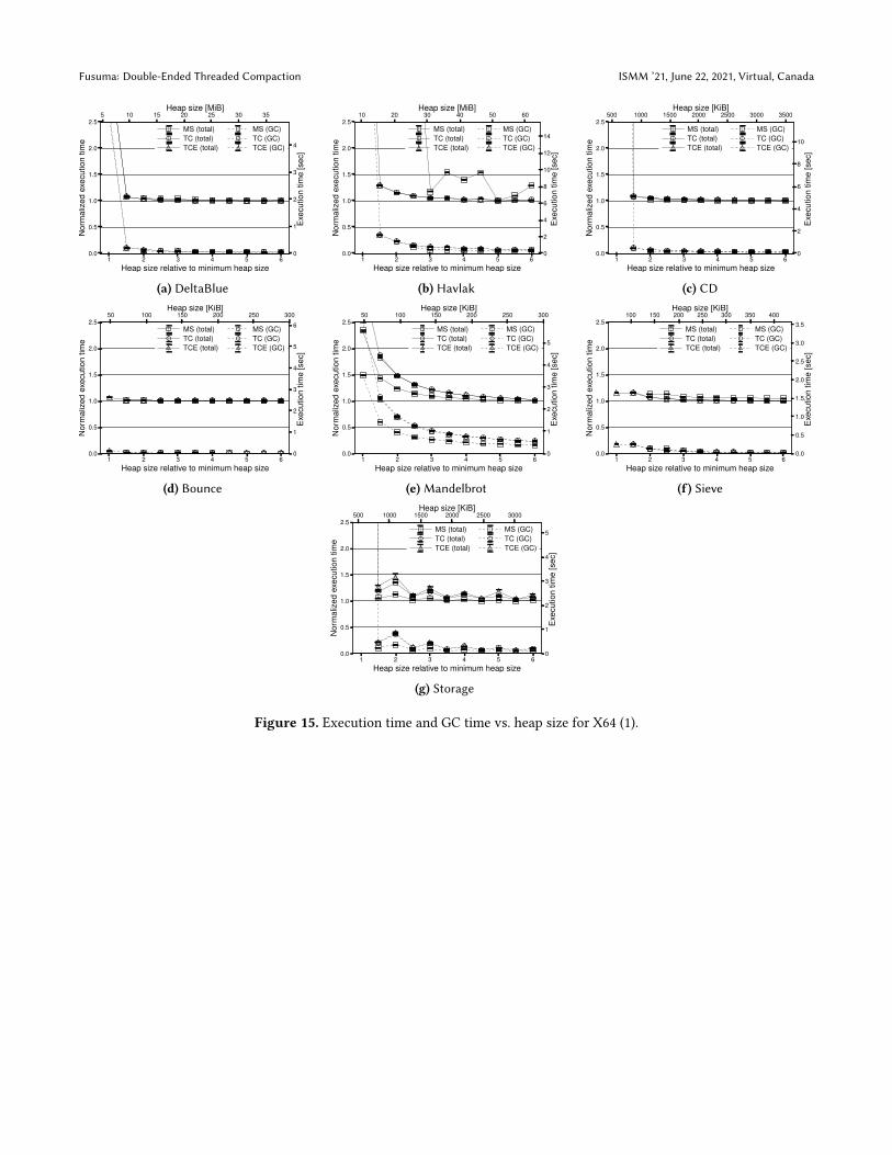
B Benchmark ResultsFigures 15 to 18 plot the execution time and the GC timeagainst the heap size for all benchmarks.

https://doi.org/10.1147/sj.442.0399

https://doi.org/10.1147/sj.442.0399

https://doi.org/10.1145/780732.780744

https://doi.org/10.1109/ICSE.2004.1317436

https://doi.org/10.1109/ICSE.2004.1317436

https://doi.org/10.1145/74877.74884

https://doi.org/10.1145/362790.362798

https://doi.org/10.1145/362790.362798

https://doi.org/10.1145/2754169.2754181

https://doi.org/10.1145/2754169.2754181

https://doi.org/10.1145/3315573.3329978

https://doi.org/10.1145/1029873.1029879

https://doi.org/10.1145/800017.800542

https://doi.org/10.1093/comjnl/10.2.162

https://doi.org/10.1007/BFb0057013

https://doi.org/10.1016/0020-0190(79)90103-0

https://doi.org/10.1016/0020-0190(79)90103-0

https://doi.org/10.1145/1133981.1134023

https://doi.org/10.1145/1133981.1134023

https://www.worldcat.org/oclc/312910844

https://www.worldcat.org/oclc/312910844

https://doi.org/10.1145/29650.29677

https://doi.org/10.1145/29650.29677

https://doi.org/10.1145/2989225.2989232

http://www.usenix.org/publications/library/proceedings/jvm01/printezis.html

http://www.usenix.org/publications/library/proceedings/jvm01/printezis.html

https://doi.org/10.1016/j.cola.2019.01.003

https://doi.org/10.1016/j.cola.2019.01.003

https://doi.org/10.1145/3226225



0.0

0.5

1.0

1.5

2.0

2.5

Nor

mal

ized

exec

utio

ntim

e



5 10 15 20 25 30 35Heap size [MiB]

0

1

2

3

4

Exe

cutio

ntim

e[s

ec]

(a) DeltaBlue


0.0

0.5

1.0

1.5

2.0

2.5

Nor

mal

ized

exec

utio

ntim

e



10 20 30 40 50 60Heap size [MiB]

0

2

4

6

8

10

12

14

Exe

cutio

ntim

e[s

ec]

(b) Havlak


0.0

0.5

1.0

1.5

2.0

2.5

Nor

mal

ized

exec

utio

ntim

e



500 1000 1500 2000 2500 3000 3500Heap size [KiB]

0

2

4

6

8

10

Exe

cutio

ntim

e[s

ec]

(c) CD


0.0

0.5

1.0

1.5

2.0

2.5

Nor

mal

ized

exec

utio

ntim

e



50 100 150 200 250 300Heap size [KiB]

0

1

2

3

4

5

6

Exe

cutio

ntim

e[s

ec]

(d) Bounce


0.0

0.5

1.0

1.5

2.0

2.5

Nor

mal

ized

exec

utio

ntim

eMS (total)TC (total)TCE (total)


50 100 150 200 250 300Heap size [KiB]

0

1

2

3

4

5

Exe

cutio

ntim

e[s

ec]

(e) Mandelbrot


0.0

0.5

1.0

1.5

2.0

2.5

Nor

mal

ized

exec

utio

ntim

e



100 150 200 250 300 350 400Heap size [KiB]

0.0

0.5

1.0

1.5

2.0

2.5

3.0

3.5

Exe

cutio

ntim

e[s

ec]

(f) Sieve


0.0

0.5

1.0

1.5

2.0

2.5

Nor

mal

ized

exec

utio

ntim

e



500 1000 1500 2000 2500 3000Heap size [KiB]

0

1

2

3

4

5

Exe

cutio

ntim

e[s

ec]

(g) Storage

Figure 15. Execution time and GC time vs. heap size for X64 (1).



0.0

0.5

1.0

1.5

2.0

2.5

Nor

mal

ized

exec

utio

ntim

e



50 100 150 200 250Heap size [KiB]

0

1

2

3

4

5

Exe

cutio

ntim

e[s

ec]

(a) 3d-cube


0.0

0.5

1.0

1.5

2.0

2.5

Nor

mal

ized

exec

utio

ntim

e



500 1000 1500 2000 2500 3000 3500Heap size [KiB]

0

1

2

3

4

5

Exe

cutio

ntim

e[s

ec]

(b) 3d-morph


0.0

0.5

1.0

1.5

2.0

2.5

Nor

mal

ized

exec

utio

ntim

e



50 100 150 200 250Heap size [KiB]

0

1

2

3

4

Exe

cutio

ntim

e[s

ec]

(c) access-binary-trees


0.0

0.5

1.0

1.5

2.0

2.5

Nor

mal

ized

exec

utio

ntim

e



50 100 150 200 250Heap size [KiB]

0.0

0.5

1.0

1.5

2.0

2.5

3.0

3.5

4.0

Exe

cutio

ntim

e[s

ec]

(d) access-nbody


0.0

0.5

1.0

1.5

2.0

2.5

Nor

mal

ized

exec

utio

ntim



50 100 150 200 250Heap size [KiB]

0

1

2

3

4

5

6

Exe

cutio

ntim

e[s

ec]

(e) math-partial-sums


0.0

0.5

1.0

1.5

2.0

2.5

Nor

mal

ized

exec

utio

ntim

e



50 100 150 200 250Heap size [KiB]

0

1

2

3

4

5

6

7

8

Exe

cutio

ntim

e[s

ec]

(f) math-spectral-norm


0.0

0.5

1.0

1.5

2.0

2.5

Nor

mal

ized

exec

utio

ntim

e



100 200 300 400 500 600Heap size [KiB]

0

1

2

3

4

5

Exe

cutio

ntim

e[s

ec]

(g) string-base64


0.0

0.5

1.0

1.5

2.0

2.5

Nor

mal

ized

exec

utio

ntim

e



50 100 150 200 250Heap size [KiB]

0

1

2

3

4

5

6

7

8

Exe

cutio

ntim

e[s

ec]

(h) string-fasta


0.0

0.5

1.0

1.5

2.0

2.5

Nor

mal

ized

exec

utio

ntim

e



50 100 150 200 250 300Heap size [KiB]

0

1

2

3

4

5

6

Exe

cutio

ntim

e[s

ec]

(i) dht11


0.0

0.5

1.0

1.5

2.0

2.5

Nor

mal

ized

exec

utio

ntim

e



100 200 300 400 500 600 700Heap size [KiB]

0.00

0.25

0.50

0.75

1.00

1.25

1.50

1.75

2.00

Exe

cutio

ntim

e[s

ec]

(j) inc-prop

Figure 16. Execution time and GC time vs. heap size for X64 (2).



0.0

0.5

1.0

1.5

2.0

2.5

Nor

mal

ized

exec

utio

ntim

e



4 6 8 10 12 14 16 18Heap size [MiB]

0

5

10

15

20

25

30

35

Exe

cutio

ntim

e[s

ec]

(a) DeltaBlue


0.0

0.5

1.0

1.5

2.0

2.5

Nor

mal

ized

exec

utio

ntim

e



5 10 15 20 25 30Heap size [MiB]

0

20

40

60

80

100

Exe

cutio

ntim

e[s

ec]

(b) Havlak


0.0

0.5

1.0

1.5

2.0

2.5

Nor

mal

ized

exec

utio

ntim

e



400 600 800 1000 1200 1400 1600 1800Heap size [KiB]

0

10

20

30

40

50

60

70

80

Exe

cutio

ntim

e[s

ec]

(c) CD


0.0

0.5

1.0

1.5

2.0

2.5

Nor

mal

ized

exec

utio

ntim

e



40 60 80 100 120 140 160Heap size [KiB]

0

10

20

30

40

Exe

cutio

ntim

e[s

ec]

(d) Bounce


0.0

0.5

1.0

1.5

2.0

2.5

Nor

mal

ized

exec

utio

ntim



20 40 60 80 100 120 140 160Heap size [KiB]

0

5

10

15

20

25

30

Exe

cutio

ntim

e[s

ec]

(e) Mandelbrot


0.0

0.5

1.0

1.5

2.0

2.5

Nor

mal

ized

exec

utio

ntim

e



50 75 100 125 150 175 200 225Heap size [KiB]

0

5

10

15

20

25

30

Exe

cutio

ntim

e[s

ec]

(f) Sieve


0.0

0.5

1.0

1.5

2.0

2.5

Nor

mal

ized

exec

utio

ntim

e



400 600 800 1000 1200 1400 1600Heap size [KiB]

0

5

10

15

20

25

30

35

Exe

cutio

ntim

e[s

ec]

(g) Storage

Figure 17. Execution time and GC time vs. heap size for RP (1).



0.0

0.5

1.0

1.5

2.0

2.5

Nor

mal

ized

exec

utio

ntim

e



20 40 60 80 100 120 140 160Heap size [KiB]

0

5

10

15

20

25

30

Exe

cutio

ntim

e[s

ec]

(a) 3d-cube


0.0

0.5

1.0

1.5

2.0

2.5

Nor

mal

ized

exec

utio

ntim

e



500 750 1000 1250 1500 1750 2000 2250Heap size [KiB]

0

5

10

15

20

25

30

35

Exe

cutio

ntim

e[s

ec]

(b) 3d-morph


0.0

0.5

1.0

1.5

2.0

2.5

Nor

mal

ized

exec

utio

ntim

e



20 40 60 80 100 120 140Heap size [KiB]

0

5

10

15

20

25

30

35

Exe

cutio

ntim

e[s

ec]

(c) access-binary-trees


0.0

0.5

1.0

1.5

2.0

2.5

Nor

mal

ized

exec

utio

ntim

e



20 40 60 80 100 120 140 160Heap size [KiB]

0

5

10

15

20

25

Exe

cutio

ntim

e[s

ec]

(d) access-nbody


0.0

0.5

1.0

1.5

2.0

2.5

Nor

mal

ized

exec

utio

ntim



20 40 60 80 100 120 140Heap size [KiB]

0

5

10

15

20

25

30

35

40

Exe

cutio

ntim

e[s

ec]

(e) math-partial-sums


0.0

0.5

1.0

1.5

2.0

2.5

Nor

mal

ized

exec

utio

ntim

e



20 40 60 80 100 120 140Heap size [KiB]

0

10

20

30

40

50

Exe

cutio

ntim

e[s

ec]

(f) math-spectral-norm


0.0

0.5

1.0

1.5

2.0

2.5

Nor

mal

ized

exec

utio

ntim

e



100 200 300 400 500Heap size [KiB]

0

2

4

6

8

10

12

14

16

Exe

cutio

ntim

e[s

ec]

(g) string-base64


0.0

0.5

1.0

1.5

2.0

2.5

Nor

mal

ized

exec

utio

ntim

e



20 40 60 80 100 120 140 160Heap size [KiB]

0

10

20

30

40

50

Exe

cutio

ntim

e[s

ec]

(h) string-fasta


0.0

0.5

1.0

1.5

2.0

2.5

Nor

mal

ized

exec

utio

ntim

e



40 60 80 100 120 140 160Heap size [KiB]

0

10

20

30

40

Exe

cutio

ntim

e[s

ec]

(i) dht11


0.0

0.5

1.0

1.5

2.0

2.5

Nor

mal

ized

exec

utio

ntim

e



50 100 150 200 250 300 350Heap size [KiB]

0

2

4

6

8

10

12

14

16

Exe

cutio

ntim

e[s

ec]

(j) inc-prop

Figure 18. Execution time and GC time vs. heap size for RP (2).

Fusuma: Double-Ended Threaded Compaction(Full Version)

Documents

Transcript of Fusuma: Double-Ended Threaded Compaction(Full Version)