Fundamentals of prediction

patterns, predictions, and actions - 2021-10-20 1

2

Fundamentals of prediction

Prediction is the art and science of leveraging patterns found innatural and social processes to conjecture about uncertain events. Weuse the word prediction broadly to refer to statements about things wedon’t know for sure yet, including but not limited to the outcome offuture events.

Machine learning is to a large extent the study of algorithmicprediction. Before we can dive into machine learning, we shouldfamiliarize ourselves with prediction. Starting from first principles,we will motivate the goals of prediction before building up to astatistical theory of prediction.

We can formalize the goal of prediction problems by assuming apopulation of N instances with a variety of attributes. We associatewith each instance two variables, denoted X and Y. The goal ofprediction is to conjecture a plausible value for Y after observing Xalone. But when is a prediction good? For that, we must quantifysome notion of the quality of prediction and aim to optimize thatquantity.

To start, suppose that for each variable X we make a deterministicprediction f (X) by means of some prediction function f . A naturalgoal is to find a function f that makes the fewest number of incorrectpredictions, where f (X) 6= Y, across the population. We can thinkof this function as a computer program that reads X as input andoutputs a prediction f (X) that we hope matches the value Y. For afixed prediction function, f , we can sum up all of the errors made onthe population. Dividing by the size of the population, we observethe average (or mean) error rate of the function.

Minimizing errors

Let’s understand how we can find a prediction function that makesas few errors as possible on a given population in the case of binaryprediction, where the variable Y has only two values.

Consider a population of Abalone, a type of marine snail withcolorful shells featuring a varying number of rings. Our goal is topredict the sex, male or female, of the Abalone from the number ofrings on the shell. We can tabulate the population of Abalone bycounting for each possible number of rings, the number of male and

2 moritz hardt and benjamin recht

female instances in the population.

0 1 2 3 4 5 6 7 8 9 10 11 12 13 14 15 16 17 18 19 20 21 22 23Number of rings

0

50

100

150

200

250

Num

ber

ofin

stan

ces

Abalone sea snails

male

female

Figure 1: Predicting the sex of Abalonesea snails

From this way of presenting the population, it is not hard to com-pute the predictor that makes the fewest mistakes. For each valueon the X-axis, we predict “female” if the number of female instanceswith this X-value is larger than the number of male instances. Other-wise, we predict “male” for the given X-value. For example, there’sa majority of male Abalone with seven rings on the shell. Hence, itmakes sense to predict “male” when we see seven rings on a shell.Scrutinizing the figure a bit further, we can see that the best possiblepredictor is a threshold function that returns “male” whenever thenumber of rings is at most 8, and “female” whenever the number ofrings is greater or equal to 9.

The number of mistakes our predictor makes is still significant.After all, most counts are pretty close to each other. But it’s betterthan random guessing. It uses whatever there is that we can say fromthe number of rings about the sex of an Abalone snail, which is justnot much.

What we constructed here is called the minimum error rule. Itgeneralizes to multiple attributes. If we had measured not only thenumber of rings, but also the length of the shell, we would repeat theanalogous counting exercise over the two-dimensional space of allpossible values of the two attributes.

The minimum error rule is intuitive and simple, but computingthe rule exactly requires examining the entire population. Trackingdown every instance of a population is not only intractable. It alsodefeats the purpose of prediction in almost any practical scenario.


If we had a way of enumerating the X and Y value of all instancesin a population, the prediction problem would be solved. Given aninstance X we could simply look up the corresponding value of Yfrom our records.

What’s missing so far is a way of doing prediction that does notrequire us to enumerate the entire population of interest.

Modeling knowledge

Fundamentally, what makes prediction without enumeration possibleis knowledge about the population. Human beings organize andrepresent knowledge in different ways. In this chapter, we willexplore in depth the consequences of one particular way to representpopulations, specifically, as probability distributions.

The assumption we make is that we have knowledge of a proba-bility distribution p(x, y) over pairs of X and Y values. We assumethat this distribution conceptualizes the “typical instance” in a popu-lation. If we were to select an instance uniformly at random from thepopulation, what relations between its attributes might we expect?We expect that a uniform sample from our population would be thesame as a sample from p(x, y). We call such a distribution a statisticalmodel or simply model of a population. The word model emphasizesthat the distribution isn’t the population itself. It is, in a sense, asketch of a population that we use to make predictions.

Let’s revisit our Abalone example in probabilistic form. Assumewe know the distribution of the number of rings of male and femaleAbalone, as illustrated in the figure.

Both follow a skewed normal distribution described by three pa-rameters each, a location, a scale, and a skew parameter. Knowingthe distribution is to assume that we know these parameters. Al-though the specific numbers won’t matter for our example, let’s spellthem out for concreteness. The distribution for male Abalone haslocation 7.4, scale 4.48, and skew 3.12, whereas the distribution forfemale Abalone has location 7.63, scale 4.67, and skew 4.34. To com-plete the specification of the joint distribution over X and Y, we needto determine the relative proportion of males and females. Assumefor this example that male and female Abalone are equally likely.

Representing the population this way, it makes sense to predict“male” whenever the probability density for male Abalone is largerthan that for female Abalone. By inspecting the plot we can see thatthe density is higher for male snails up until 8 rings at which pointit is larger for female instances. We can see that the predictor wederive from this representation is the same threshold rule that wehad before.


0 1 2 3 4 5 6 7 8 9 10 11 12 13 14 15 16 17 18 19 20 21 22 23Number of rings

0.000

0.025

0.050

0.075

0.100

0.125

0.150

Prob

abili

tyde

nsit

yAbalone sea snails

male

female

Figure 2: Representing Abalone popula-tion as a distribution

We arrived at the same result without the need to enumerate andcount all possible instances in the population. Instead, we recoveredthe minimum error rule from knowing only 7 parameters, three foreach conditional distribution, and one for the balance of the twoclasses.

Modeling populations as probability distributions is an importantstep in making prediction algorithmic. It allows us to representpopulations succinctly, and gives us the means to make predictionsabout instances we haven’t encountered.

Subsequent chapters extend these fundamentals of predictionto the case where we don’t know the exact probability distribution,but only have a random sample drawn from the distribution. It istempting to think about machine learning as being all about that,namely what we do with a sample of data drawn from a distribution.However, as we learn in this chapter, many fundamentally importantquestions arise even if we have full knowledge of the population.

Prediction from statistical models

Let’s proceed to formalize prediction assuming we have full knowl-edge of a statistical model of the population. Our first goal is toformally develop the minimum error rule in greater generality.

We begin with binary prediction where we suppose Y has twoalternative values, 0 and 1. Given some measured information X, ourgoal is to conjecture whether Y equals zero or one.

Throughout we assume that X and Y are random variables drawn


from a joint probability distribution. It is convenient both mathemati-cally and conceptually to specify the joint distribution as follows. Weassume that Y has a priori (or prior) probabilities:

p0 = P[Y = 0] , p1 = P[Y = 1]

That is, the we assume we know the proportion of instances with Y =

1 and Y = 0 in the population. We’ll always model available informa-tion as being a random vector X with support in Rd. Its distributiondepends on whether Y is equal to zero or one. In other words, thereare two different statistical models for the data, one for each valueof Y. These models are the conditional probability densities of Xgiven a value y for Y, denoted p(x | Y = y). This density function isoften called a generative model or likelihood function for each scenario.

Example: Signal versus noise

For a simple example with more mathematical formalism, sup-pose that when Y = 0 we observe a scalar X = ω where ω isunit-variance, zero mean gaussian noise ω ∼ N (0, 1). Recall thatthe gaussian distribution of mean µ and variance σ2 is given by the

density 1σ√

2πe−

12 (

x−µσ )

2

.Suppose when Y = 1, we would observe X = s + ω for some

scalar s. That is, the conditional densities are

p(x | Y = 0) = N (0, 1) ,

p(x | Y = 1) = N (s, 1) .

The larger the shift s is, the easier it is to predict whether Y = 0or Y = 1. For example, suppose s = 10 and we observed X = 11.If we had Y = 0, the probability that the observation is greaterthan 10 is on the order of 10−23, and hence we’d likely think we’rein the alternative scenario where Y = 1. However, if s were veryclose to zero, distinguishing between the two alternatives is ratherchallenging. We can think of a small difference s that we’re trying todetect as a needle in a haystack.

Prediction via optimization

Our core approach to all statistical decision making will be to for-mulate an appropriate optimization problem for which the decisionrule is the optimal solution. That is, we will optimize over algorithms,searching for functions that map data to decisions and predictions.We will define an appropriate notion of the cost associated to eachdecision, and attempt to construct decision rules that minimize the


−5.0 −2.5 0.0 2.5 5.0

0.0

0.1

0.2

0.3

0.4Overlapping gaussians

H0

H1

−10 −5 0 5 10

0.0

0.1

0.2

0.3

0.4Well-separated gaussians

H0

H1

Figure 3: Illustration of shifted gaus-sians

expected value of this cost. As we will see, choosing this optimizationframework has many immediate consequences.

Predictors and labels

A predictor is a function Y(x) that maps an input x to a prediction y =

Y(x). The prediction y is also called a label for the point x. The targetvariable Y can be both real valued or discrete. When Y is a discreterandom variable, each different value it can take on is called a class ofthe prediction problem.

To ease notation, we take the liberty to write Y as a shorthand forthe random variable Y(X) that we get by applying the predictionfunction Y to the random variable X.

The most common case we consider through the book is binaryprediction, where we have two classes, 0 and 1. Sometimes it’s mathe-matically convenient to instead work with the numbers −1 and 1 forthe two classes.

In most cases we consider, labels are scalars that are either discreteor real-valued. Sometimes it also makes sense to consider vector-valued predictions and target variables.

The creation and encoding of suitable labels for a predictionproblem is an important step in applying machine learning to realworld problems. We will return to it multiple times.

Loss functions and risk

The final ingredient in our formal setup is a loss function whichgeneralizes the notion of an error that we defined as a mismatchbetween prediction and target value.

A loss function takes two inputs, y and y, and returns a real num-ber loss(y, y) that we interpret as a quantified loss for predicting ywhen the target is y. A loss could be negative in which case we thinkof it as a reward.


A prediction error corresponds to the loss function loss(y, y) =

1{y 6= y} that indicates disagreement between its two inputs. Lossfunctions give us modeling flexibility that will become crucial as weapply this formal setup throughout this book.

An important notion is the expected loss of a predictor taken overa population. This construct is called risk.

Definition 1. We define the risk associated with Y to be

R[Y] := E[loss(Y(X), Y)] .

Here, the expectation is taken jointly over X and Y.

Now that we defined risk, our goal is to determine which decisionrule minimizes risk. Let’s get a sense for how we might go about this.

In order to minimize risk, theoretically speaking, we need to solvean infinite dimensional optimization problem over binary-valuedfunctions. That is, for every x, we need to find a binary assignment.Fortunately, the infinite dimension here turns out to not be a problemanalytically once we make use of the law of iterated expectation.

Lemma 1. We claim that the optimal predictor is given by

Y(x) = 1

{P[Y = 1 | X = x] ≥ loss(1, 0)− loss(0, 0)

loss(0, 1)− loss(1, 1) P[Y = 0 | X = x]}

.

This rule corresponds to the intuitive rule we derived when think-ing about how to make predictions over the population. For a fixedvalue of the data X = x, we compare the frequency of which Y = 1occurs to which Y = 0 occurs. If this frequency exceeds some thresh-old that is defined by our loss function, then we set Y(x) = 1. Other-wise, we set Y(x) = 0.

Proof. To see why this is rule is optimal, we make use of the law ofiterated expectation:

E[loss(Y(X), Y)] = E

[E

[loss(Y(X), Y) | X

]].

Here, the outer expectation is over a random draw of X and theinner expectation samples Y conditional on X. Since there are noconstraints on the predictor Y, we can minimize the expression byminimizing the inner expectation independently for each possiblesetting that X can assume.

Indeed, for a fixed value x, we can expand the expected loss foreach of the two possible predictions:

E[loss(0, Y) | X = x] = loss(0, 0)P[Y = 0 | X = x] + loss(0, 1)P[Y = 1 | X = x]

E[loss(1, Y) | X = x] = loss(1, 0)P[Y = 0 | X = x] + loss(1, 1)P[Y = 1 | X = x] .


The optimal assignment for this x is to set Y(x) = 1 whenever thesecond expression is smaller than the first. Writing out this inequalityand rearranging gives us the rule specified in the lemma.

Probabilities of the form P[Y = y | X = x], as they appeared in thelemma, are called posterior probability.

We can relate them to the likelihood function via Bayes rule:

P[Y = y | X = x] =p(x | Y = y)py

p(x),

where p(x) is a density function for the marginal distribution of X.When we use posterior probabilities, we can rewrite the optimal

predictor as

Y(x) = 1

{p(x | Y = 1)p(x | Y = 0)

≥ p0(loss(1, 0)− loss(0, 0))p1(loss(0, 1)− loss(1, 1))

}.

This rule is an example of a likelihood ratio test.

Definition 2. The likelihood ratio is the ratio of the likelihood functions:

L(x) :=p(x | Y = 1)p(x | Y = 0)

A likelihood ratio test (LRT) is a predictor of the form

Y(x) = 1{L(x) ≥ η}

for some scalar threshold η > 0.

If we denote the optimal threshold value

η =p0(loss(1, 0)− loss(0, 0))p1(loss(0, 1)− loss(1, 1))

, (1)

then the predictor that minimizes the risk is the likelihood ratio test

Y(x) = 1{L(x) ≥ η} .

A LRT naturally partitions the sample space in two regions:

X0 = {x ∈ X : L(x) ≤ η}X1 = {x ∈ X : L(x) > η} .

The sample space X then becomes the disjoint union of X0 and X1.Since we only need to identify which set x belongs to, we can use anyfunction h : X → R which gives rise to the same threshold rule. Aslong as h(x) ≤ t whenever L(x) ≤ η and vice versa, these functions


give rise to the same partition into X0 and X1. So, for example, if g isany monotonically increasing function, then the predictor

Yg(x) = 1{g(L(x)) ≥ g(η)}

is equivalent to using Y(x). In particular, it’s popular to use thelogarithmic predictor

Ylog(x) = 1{log p(x | Y = 1)− log p(x | Y = 0) ≥ log(η)} ,

as it is often more convenient or numerically stable to work withlogarithms of likelihoods.

This discussion shows that there are an infinite number of functionswhich give rise to the same binary predictor. Hence, we don’t needto know the conditional densities exactly and can still compute theoptimal predictor. For example, suppose the true partitioning of thereal line under an LRT is

X0 = {x : x ≥ 0} and X1 = {x : x < 0} .

Setting the threshold to t = 0, the functions h(x) = x or h(x) = x3

give the same predictor, as does any odd function which is positiveon the right half line.

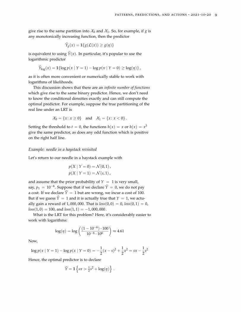
Example: needle in a haystack revisited

Let’s return to our needle in a haystack example with

p(X | Y = 0) = N (0, 1) ,

p(X | Y = 1) = N (s, 1) ,

and assume that the prior probability of Y = 1 is very small,say, p1 = 10−6. Suppose that if we declare Y = 0, we do not paya cost. If we declare Y = 1 but are wrong, we incur a cost of 100.But if we guess Y = 1 and it is actually true that Y = 1, we actu-ally gain a reward of 1, 000, 000. That is loss(0, 0) = 0, loss(0, 1) = 0,loss(1, 0) = 100, and loss(1, 1) = −1, 000, 000 .

What is the LRT for this problem? Here, it’s considerably easier towork with logarithms:

log(η) = log((1− 10−6) · 100

10−6 · 106

)≈ 4.61

Now,

log p(x | Y = 1)− log p(x | Y = 0) = −12(x− s)2 +

12

x2 = sx− 12

s2

Hence, the optimal predictor is to declare

Y = 1{

sx > 12 s2 + log(η)

}.


The optimal rule here is linear. Moreover, the rule divides the spaceinto two open intervals. While the entire real line lies in the unionof these two intervals, it is exceptionally unlikely to ever see an xlarger than |s|+ 5. Hence, even if our predictor were incorrect in theseregions, the risk would still be nearly optimal as these terms havealmost no bearing on our expected risk!

Canonical cases of likelihood ratio tests

A folk theorem of statistical decision theory states that essentially alloptimal rules are equivalent to likelihood ratio tests. While this isn’talways true, many important prediction rules end up being equivalentto LRTs. Shortly, we’ll see an optimization problem that speaks to thepower of LRTs. But before that, we can already show that the wellknown maximum likelihood and maximum a posteriori predictors areboth LRTs.

Maximum a posteriori rule

The expected error of a predictor is the expected number of timeswe declare Y = 0 (resp. Y = 1) when Y = 1 (resp. Y = 0) istrue. Minimizing the error is equivalent to minimizing the risk withcost loss(0, 0) = loss(1, 1) = 0, loss(1, 0) = loss(0, 1) = 1. The optimumpredictor is hence a likelihood ratio test. In particular,

Y(x) = 1{L(x) ≥ p0

p1

}.

Using Bayes rule, one can see that this rule is equivalent to

Y(x) = arg maxy∈{0,1}

P[Y = y | X = x] .

Recall that the expression P[Y = y | X = x] is called the posteriorprobability of Y = y given X = x. And this rule is hence referred toas the maximum a posteriori (MAP) rule.

Maximum likelihood rule

As we discussed above, the expression p(x | Y = y) is called thelikelihood of the point x given the class Y = y. A maximum likelihoodrule would set

Y(x) = arg maxy

p(x | Y = y) .

This is completely equivalent to the LRT when p0 = p1 and the costsare loss(0, 0) = loss(1, 1) = 0, loss(1, 0) = loss(0, 1) = 1. Hence,the maximum likelihood rule is equivalent to the MAP rule with auniform prior on the labels.


That both of these popular rules ended up reducing to LRTs is noaccident. In what follows, we will show that LRTs are almost alwaysthe optimal solution of optimization-driven decision theory.

Types of errors and successes

Let Y(x) denote any predictor mapping into {0, 1}. Binary predic-tions can be right or wrong in four different ways summarized by theconfusion table.

Table 1: Confusion table

Y = 0 Y = 1

Y = 0 true negative false negativeY = 1 false positive true positive

Taking expected values over the populations give us four corre-sponding rates that are characteristics of a predictor.

1. True Positive Rate: TPR = P[Y(X) = 1 | Y = 1]. Also known aspower, sensitivity, probability of detection, or recall.

2. False Negative Rate: FNR = 1− TPR. Also known as type II erroror probability of missed detection.

3. False Positive Rate: FPR = P[Y(X) = 1 | Y = 0]. Also known assize or type I error or probability of false alarm.

4. True Negative Rate TNR = 1− FPR, the probability of declaringY = 0 given Y = 0. This is also known as specificity.

There are other quantities that are also of interest in statistics andmachine learning:

1. Precision: P[Y = 1 | Y(X) = 1]. This is equal to (p1TPR)/(p0FPR +

p1TPR).2. F1-score: F1 is the harmonic mean of precision and recall. We can

write this asF1 =

2TPR1 + TPR + p0

p1FPR

3. False discovery rate: False discovery rate (FDR) is equal to theexpected ratio of the number of false positives to the total numberof positives.

In the case where both labels are equally likely, precision, F1,and FDR are also only functions of FPR and TPR. However, thesequantities explicitly account for class imbalances: when there is a sig-nificant skew between p0 and p1, such measures are often preferred.


TPR and FPR are competing objectives. We’d like TPR as large aspossible and FPR as small as possible.

We can think of risk minimization as optimizing a balance be-tween TPR and FPR:

R[Y] := E[loss(Y(X), Y)] = αFPR− βTPR + γ ,

where α and β are nonnegative and γ is some constant. For allsuch α, β, and γ, the risk-minimizing predictor is an LRT.

Other cost functions might try to balance TPR versus FPR in otherways. Which pairs of (FPR, TPR) are achievable?

ROC curves

True and false positive rate lead to another fundamental notion,called the the receiver operating characteristic (ROC) curve.

The ROC curve is a property of the joint distribution (X, Y) andshows for every possible value α = [0, 1] the best possible truepositive rate that we can hope to achieve with any predictor that hasfalse positive rate α. As a result the ROC curve is a curve in the FPR-TPR plane. It traces out the maximal TPR for any given FPR. Clearlythe ROC curve contains values (0, 0) and (1, 1), which are achievedby constant predictors that either reject or accept all inputs.

0.0 0.5 1.0False positive rate

0.0

0.5

1.0

True

posi

tive

rate

ROC curveFigure 4: Example of an ROC curve

We will now show, in a celebrated result by Neyman and Pear-son, that the ROC curve is given by varying the threshold in thelikelihood ratio test from negative to positive infinity.

The Neyman-Pearson Lemma

The Neyman-Pearson Lemma, a fundamental lemma of decisiontheory, will be an important tool for us to establish three importantfacts. First, it will be a useful tool for understanding the geometric


properties of ROC curves. Second, it will demonstrate another im-portant instance where an optimal predictor is a likelihood ratio test.Third, it introduces the notion of probabilistic predictors.

Suppose we want to maximize true positive rate subject to anupper bound on the false positive rate. That is, we aim to solve theoptimization problem:

maximize TPRsubject to FPR ≤ α

Let’s optimize over probabilistic predictors. A probabilistic predic-tor Q returns 1 with probability Q(x) and 0 with probability 1−Q(x).With such rules, we can rewrite our optimization problem as:

maximizeQ E[Q(X) | Y = 1]subject to E[Q(X) | Y = 0] ≤ α

∀x : Q(x) ∈ [0, 1]

Lemma 2. Neyman-Pearson Lemma. Suppose the likelihood func-tions p(x|Y) are continuous. Then the optimal probabilistic predictor thatmaximizes TPR with an upper bound on FPR is a deterministic likelihoodratio test.

Even in this constrained setup, allowing for more powerful prob-abilistic rules, we can’t escape likelihood ratio tests. The Neyman-Pearson Lemma has many interesting consequences in its own rightthat we will discuss momentarily. But first, let’s see why the lemma istrue.

The key insight is that for any LRT, we can find a loss function forwhich it is optimal. We will prove the lemma by constructing such aproblem, and using the associated condition of optimality.

Proof. Let η be the threshold for an LRT such that the predictor

Qη(x) = 1{L(x) > η}

has FPR = α. Such an LRT exists because we assumed our likelihoodswere continuous. Let β denote the TPR of Qη .

We claim that Qη is optimal for the risk minimization problemcorresponding to the loss function

loss(1, 0) = ηp1p0

, loss(0, 1) = 1, loss(1, 1) = 0, loss(0, 0) = 0 .

Indeed, recalling Equation 1, the risk minimizer for this loss functioncorresponds to a likelihood ratio test with threshold value

p0(loss(1, 0)− loss(0, 0))p1(loss(0, 1)− loss(1, 1))

=p0loss(1, 0)p1loss(0, 1)

= η .


Moreover, under this loss function, the risk of a predictor Q equals

R[Q] = p0FPR(Q)loss(1, 0) + p1(1− TPR(Q))loss(0, 1)

= p1ηFPR(Q) + p1(1− TPR(Q)) .

Now let Q be any other predictor with FPR(Q) ≤ α. We have bythe optimality of Qη that

p1ηα + p1(1− β) ≤ p1ηFPR(Q) + p1(1− TPR(Q))

≤ p1ηα + p1(1− TPR(Q)) ,

which implies TPR(Q) ≤ β. This in turn means that Qη maxi-mizes TPR for all rules with FPR ≤ α, proving the lemma.

Properties of ROC curves

A specific randomized predictor that is useful for analysis combinestwo other rules. Suppose predictor one yields (FPR(1), TPR(1)) andthe second rule achieves (FPR(2), TPR(2)). If we flip a biased coin anduse rule one with probability p and rule 2 with probability 1− p, thenthis yields a randomized predictor with (FPR, TPR) = (pFPR(1) +

(1− p)FPR(2), pTPR(1) + (1− p)TPR(2)). Using this rule lets us proveseveral properties of ROC curves.

Proposition 1. The points (0, 0) and (1, 1) are on the ROC curve.

Proof. This proposition follows because the point (0, 0) is achievedwhen the threshold η = ∞ in the likelihood ratio test, correspondingto the constant 0 predictor. The point (1, 1) is achieved when η = 0,corresponding to the constant 1 predictor.

Proposition 2. The ROC must lie above the main diagonal.

Proof. To see why this proposition is true, fix some α > 0. Using arandomized rule, we can achieve a predictor with TPR = FPR = α.But the Neyman-Pearson LRT with FPR constrained to be less thanor equal to α achieves true positive rate greater than or equal to therandomized rule.

Proposition 3. The ROC curve is concave.

Proof. Suppose (FPR(η1), TPR(η1)) and (FPR(η2), TPR(η2)) areachievable. Then

(tFPR(η1) + (1− t)FPR(η2), tTPR(η1) + (1− t)TPR(η2))


is achievable by a randomized test. Fixing FPR ≤ tFPR(η1) +

(1 − t)FPR(η2), we see that the optimal Neyman-Pearson LRTachieves TPR ≥ TPR(η1) + (1− t)TPR(η2).

Example: the needle one more time

Consider again the needle in a haystack example, where p(x | Y =

0) = N (0, σ2) and p(x | Y = 1) = N (s, σ2) with s a positivescalar. The optimal predictor is to declare Y = 1 when X is greater

than γ := s2 +

σ2 log ηs . Hence we have

TPR =∫ ∞

γp(x | Y = 1)dx = 1

2 erfc(

γ− s√2σ

)FPR =

∫ ∞

γp(x | Y = 0)dx = 1

2 erfc(

γ√2σ

).

For fixed s and σ, the ROC curve (FPR(γ), TPR(γ)) only dependson the signal to noise ratio (SNR), s/σ. For small SNR, the ROC curveis close to the FPR = TPR line. For large SNR, TPR approaches 1 forall values of FPR.

0.0 0.2 0.4 0.6 0.8 1.0FPR

0.0

0.2

0.4

0.6

0.8

1.0

TPR SNR = 0.25

SNR = 0.5SNR = 1SNR = 2SNR = 4

Figure 5: The ROC curves for varioussignal to noise ratios in the needle inthe haystack problem.

Area under the ROC curve

Oftentimes in information retrieval and machine learning, the termROC curve is overloaded to describe the achievable FPR-TPR pairsthat we get by varying the threshold t in any predictor Y(x) =

1{R(x) > t}. Note such curves must lie below the ROC curvesthat are traced out by the optimal likelihood ratio test, but mayapproximate the true ROC curves in many cases.


A popular summary statistic for evaluating the quality of a de-cision function is the area under its associated ROC curve. This iscommonly abbreviated as AUC. In the ROC curve plotted in theprevious section, as the SNR increases, the AUC increases. However,AUC does not tell the entire story. Here we plot two ROC curveswith the same AUC.

0.0 0.2 0.4 0.6 0.8 1.0FPR

0.0

0.2

0.4

0.6

0.8

1.0

TPR

Figure 6: Two ROC curves with thesame AUC. Note that if we constrainFPR to be less than 10%, for the bluecurve, TPR can be as high as 80%whereas it can only reach 50% for thered.

If we constrain FPR to be less than 10%, for the blue curve, TPRcan be as high as 80% whereas it can only reach 50% for the red.AUC should be always viewed skeptically: the shape of an ROCcurve is always more informative than any individual number.

Looking ahead: what if we don’t know the models?

This chapter examined how to make decisions when we have accessto known probabilistic models about both data and priors about thedistribution of labels. The ubiquitous solution to decision problemsis a likelihood ratio test. But note we first derived something evensimpler: a posterior ratio test. That is, we could just compare theprobability of Y = 1 given our data to the probability of Y = 0given our data, and decide on Y = 1 if its probability was sufficientlylarger than that of Y = 0. Comparing likelihoods or posteriors areequivalent up to a rescaling of the decision threshold.

What if we don’t have a probabilistic model of how the data is gen-erated? There are two natural ways forward: Either estimate p(X | Y)from examples or estimate P[Y | X] from examples. Estimatinglikelihood models is a challenge as, when X is high dimensional,estimating p(X | Y) from data is hard in both theory and practice.Estimating posteriors on the other hand seems more promising. Esti-mating posteriors is essentially like populating an excel spreadsheet


1 Benjamin, Race After Technology (Polity,2019).

and counting places where many columns are equal to one another.But estimating the posterior is also likely overkill. We care about

the likelihood or posterior ratios as these completely govern ourpredictors. It’s possible that such ratios are easier to estimate thanthe quantities themselves. Indeed, we just need to find any functionf where f (x) ≥ 0 if p(x | Y = 1)/p(x | Y = 0) ≥ η and f (x) ≤ 0if p(x | Y = 1)/p(x | Y = 0) ≤ η. So if we only have samples

S = {(x1, y1), . . . (xn, yn)}

of data and their labels, we could try to minimize the sample average

RS[ f ] =1n

n

∑i=1

loss( f (xi), yi)

with respect to f . This approach is called empirical risk minimiza-tion (ERM) and forms the basis of most contemporary ML and AIsystems. We will devote a the next several chapters of this text tounderstanding the ins and outs of ERM.

Decisions that discriminate

The purpose of prediction is almost always decision making. Webuild predictors to guide our decision making by acting on ourpredictions. Many decisions entail a life changing event for theindividual. The decision could grant access to a major opportunity,such as college admission, or deny access to a vital resource, such asa social benefit.

Binary decision rules always draw a boundary between one groupin the population and its complement. Some are labeled accept, othersare labeled reject. When decisions have serious consequences for theindividual, however, this decision boundary is not just a technicalartifact. Rather it has moral and legal significance.

The decision maker often has access to data that encode an indi-vidual’s status in socially salient groups relating to race, ethnicity,gender, religion, or disability status. These and other categories thathave been used as the basis of adverse treatment, oppression, anddenial of opportunity in the past and in many cases to this day.

Some see formal or algorithmic decision making as a neutralmathematical tool. However, numerous scholars have shown howformal models can perpetuate existing inequities and cause harm. Inher book on this topic, Ruha Benjamin warns of

the employment of new technologies that reflect and reproduce existinginequities but that are promoted and perceived as more objective or progressivethan the discriminatory systems of a previous era.1


Even though the problems of inequality and injustice are muchbroader than one of formal decisions, we already encounter an im-portant and challenging facet within the narrow formal setup of thischapter. Specifically, we are concerned with decision rules that dis-criminate in the sense of creating an unjustified basis of differentiationbetween individuals.

A concrete example is helpful. Suppose we want to accept orreject individuals for a job. Suppose we have a perfect estimate ofthe number of hours an individual is going to work in the next 5

years. We decide that this a reasonable measure of productivity andso we accept every applicant where this number exceeds a certainthreshold. On the face of it, our rule might seem neutral. However,on closer reflection, we realize that this decision rule systematicallydisadvantages individuals who are more likely than others to makeuse of their parental leave employment benefit that our hypotheticalcompany offers. We are faced with a conundrum. On the one hand,we trust our estimate of productivity. On the other hand, we considertaking parental leave morally irrelevant to the decision we’re making.It should not be a disadvantage to the applicant. After all that isprecisely the reason why the company is offering a parental leavebenefit in the first place.

The simple example shows that statistical accuracy alone is no safe-guard against discriminatory decisions. It also shows that ignoringsensitive attributes is no safeguard either. So what then is discrimina-tion and how can we avoid it? This question has occupied scholarsfrom numerous disciplines for decades. There is no simple answer.Before we go into attempts to formalize discrimination in our sta-tistical decision making setting, it is helpful to take a step back andreflect on what the law says.

Legal background in the United States

The legal frameworks governing decision making differ from countryto country, and from one domain to another. We take a glimpse at thesituation in the United States, bearing in mind that our description isincomplete and does not transfer to other countries.

Discrimination is not a general concept. It is concerned withsocially salient categories that have served as the basis for unjustifiedand systematically adverse treatment in the past. United States lawrecognizes certain protected categories including race, sex (whichextends to sexual orientation), religion, disability status, and place ofbirth.

Further, discrimination is a domain specific concept concernedwith important opportunities that affect people’s lives. Regulated


2 Hutchinson and Mitchell, “50 Years ofTest (Un) Fairness: Lessons for MachineLearning,” in Conference on Fairness,Accountability, and Transparency, 2019,49–58.

domains include credit (Equal Credit Opportunity Act), education(Civil Rights Act of 1964; Education Amendments of 1972), employ-ment (Civil Rights Act of 1964), housing (Fair Housing Act), andpublic accommodation (Civil Rights Act of 1964). Particularly relevantto machine learning practitioners is the fact that the scope of theseregulations extends to marketing and advertising within these do-mains. An ad for a credit card, for example, allocates access to creditand would therefore fall into the credit domain.

There are different legal frameworks available to a plaintiff thatbrings forward a case of discrimination. One is called disparate treat-ment, the other is disparate impact. Both capture different forms ofdiscrimination. Disparate treatment is about purposeful consider-ation of group membership with the intention of discrimination.Disparate impact is about unjustified harm, possibly through indirectmechanisms. Whereas disparate treatment is about procedural fairness,disparate impact is more about distributive justice.

It’s worth noting that anti-discrimination law does not reflect oneoverarching moral theory. Pieces of legislation often came in responseto civil rights movements, each hard fought through decades ofactivism.

Unfortunately, these legal frameworks don’t give us a formaldefinition that we could directly apply. In fact, there is some well-recognized tension between the two doctrines.

Formal non-discrimination criteria

The idea of formal non-discrimination (or fairness) criteria goes backto pioneering work of Anne Cleary and other researchers in theeducational testing community of the 1960s.2

The main idea is to introduce a discrete random variable A thatencodes membership status in one or multiple protected classes.Formally, this random variable lives in the same probability spaceas the other covariates X, the decision Y = 1{R > t} in termsof a score R, and the outcome Y. The random variable A mightcoincide with one of the features in X or correlate strongly with somecombination of them.

Broadly speaking, different statistical fairness criteria all equalizesome group-dependent statistical quantity across groups defined bythe different settings of A. For example, we could ask to equalizeacceptance rates across all groups. This corresponds to imposing theconstraint for all groups a and b:

P[Y = 1 | A = a] = P[Y = 1 | A = b]

Researchers have proposed dozens of different criteria, each trying


3 Barocas, Hardt, and Narayanan,Fairness and Machine Learning (fairml-book.org, 2019).

4 Kleinberg, Mullainathan, and Ragha-van, “Inherent Trade-Offs in the FairDetermination of Risk Scores,” in Inno-vations in Theoretical Computer Science,2017; Chouldechova, “Fair Predictionwith Disparate Impact: A Study of Biasin Recidivism Prediction Instruments,”Big Data 5, no. 2 (2017): 153–63.

to capture different intuitions about what is fair. Simplifying thelandscape of fairness criteria, we can say that there are essentiallythree fundamentally different ones of particular significance:

• Acceptance rate P[Y = 1]• Error rates P[Y = 0 | Y = 1] and P[Y = 1 | Y = 0]• Outcome frequency given score value P[Y = 1 | R = r]

The meaning of the first two as a formal matter is clear given whatwe already covered. The third criterion needs a bit more motivation.A useful property of score functions is calibration which assertsthat P[Y = 1 | R = r] = r for all score values r. In words, wecan interpret a score value r as the propensity of positive outcomesamong instances assigned the score value r. What the third criterionsays is closely related. We ask that the score values have the samemeaning in each group. That is, instances labeled r in one group areequally likely to be positive instances as those scored r in any othergroup.

The three criteria can be generalized and simplified using threedifferent conditional independence statements.

Table 2: Non-discrimination criteria

Independence Separation Sufficiency

R ⊥ A R ⊥ A | Y Y ⊥ A | R

Each of these applies not only to binary prediction, but any setof random variables where the independence statement holds. It’snot hard to see that independence implies equality of acceptancerates across groups. Separation implies equality of error rates acrossgroups. And sufficiency implies that all groups have the same rate ofpositive outcomes given a score value.3

Researchers have shown that any two of the three criteria aremutually exclusive except in special cases. That means, generallyspeaking, imposing one criterion forgoes the other two.4

Although these formal criteria are easy to state and arguablynatural in the language of decision theory, their merit as measures ofdiscrimination has been subject of an ongoing debate.

Merits and limitations of a narrow statistical perspective

The tension between these criteria played out in a public debatearound the use of risk scores to predict recidivism in pre-trial deten-tion decisions.


5 Angwin et al., “MachineBias,” ProPublica, May 2016,https://www.propublica.org/article/

machine-bias-risk-assessments-in-criminal-sentencing.

6 Dieterich, Mendoza, and Brennan,“COMPAS Risk Scales: Demon-strating Accuracy Equity andPredictive Parity,” 2016, https://www.documentcloud.org/documents/

2998391-ProPublica-Commentary-Final-070616.

html.

7 Neyman and Pearson, “On the Useand Interpretation of Certain TestCriteria for Purposes of StatisticalInference: Part I,” Biometrika, 1928,175–240.8 Neyman and Pearson, “On the Prob-lem of the Most Efficient Tests ofStatistical Hypotheses,” PhilosophicalTransactions of the Royal Society of Lon-don. Series A 231, no. 694–706 (1933):289–337.

There’s a risk score, called COMPAS, used by many jurisdic-tions in the United States to assess risk of recidivism in pre-trial baildecisions. Recidivism refers to a person’s relapse into criminal be-havior. In the United States, a defendant may either be detainedor released on bail prior to the trial in court depending on variousfactors. Judges may detain defendants in part based on this score.

Investigative journalists at ProPublica found that Black defendantsface a higher false positive rate, i.e., more Black defendants labeledhigh risk end up not committing a crime upon release than amongWhite defendants labeled high risk.5 In other words, the COMPASscore fails the separation criterion.

A company called Northpointe, which sells the proprietary COM-PAS risk model, pointed out in return that Black and White defen-dants have equal recidivism rates given a particular score value. Thatis defendants labeled, say, an ‘8’ for high risk would go on to recidi-vate at a roughly equal rate in either group. Northpointe claimed thatthis property is desirable so that a judge can interpret scores equallyin both groups.6

The COMPAS debate illustrates both the merits and limitations ofthe narrow framing of discrimination as a classification criterion.

On the hand, the error rate disparity gave ProPublica a tangibleand concrete way to put pressure on Northpointe. The narrow fram-ing of decision making identifies the decision maker as responsiblefor their decisions. As such, it can be used to interrogate and possiblyintervene in the practices of an entity.

On the other hand, decisions are always part of a broader systemthat embeds structural patterns of discrimination. For example, ameasure of recidivism hinges crucially on existing policing patterns.Crime is only found where policing activity happens. However, theallocation and severity of police force itself has racial bias. Somescholars therefore find an emphasis on statistical criteria rather thanstructural determinants of discrimination to be limited.

Chapter notes

The theory we covered in this chapter is also called detection theoryand decision theory. Similarly, what we call a predictor throughout hasvarious different names, such as decision rule or classifier.

The elementary detection theory covered in this chapter has notchanged much at all since the 1950s and is essentially considereda “solved problem”. Neyman and Pearson invented the likelihoodratio test7 and later proved their lemma showing it to be optimalfor maximizing true positive rates while controlling false positiverates.8 Wald followed this work by inventing general Bayes risk

https://www.propublica.org/article/machine-bias-risk-assessments-in-criminal-sentencing


https://www.documentcloud.org/documents/2998391-ProPublica-Commentary-Final-070616.html





9 Wald, “Contributions to the Theoryof Statistical Estimation and TestingHypotheses,” The Annals of MathematicalStatistics 10, no. 4 (1939): 299–326.

10 Bertsekas and Tsitsiklis, Introductionto Probability, 2nd ed. (Athena Scientific,2008).11 Peterson, Birdsall, and Fox, “The The-ory of Signal Detectability,” Transactionsof the IRE 4, no. 4 (1954): 171–212.

12 Tanner Jr. and Swets, “A Decision-Making Theory of Visual Detection,”Psychological Review 61, no. 6 (1954):401.13 Chow, “An Optimum CharacterRecognition System Using DecisionFunctions,” IRE Transactions on Elec-tronic Computers, no. 4 (1957): 247–54.14 Highleyman, “Linear DecisionFunctions, with Application to PatternRecognition,” Proceedings of the IRE 50,no. 6 (1962): 1501–14.

15 Benjamin, Race After Technology.16 Broussard, Artificial Unintelligence:How Computers Misunderstand the World(MIT Press, 2018).17 Eubanks, Automating Inequality: HowHigh-Tech Tools Profile, Police, and Punishthe Poor (St. Martin’s Press, 2018).18 Noble, Algorithms of Oppression: HowSearch Engines Reinforce Racism (NYUPress, 2018).19 O’Neil, Weapons of Math Destruction:How Big Data Increases Inequality andThreatens Democracy (Broadway Books,2016).20 Barocas, Hardt, and Narayanan,Fairness and Machine Learning.

minimization in 1939.9 Wald’s ideas were widely adopted duringWorld War II for the purpose of interpreting RADAR signals whichwere often very noisy. Much work was done to improve RADARoperations, and this led to the formalization that the output of aRADAR system (the receiver) should be a likelihood ratio, and adecision should be made based on an LRT. Our proof of Neyman-Pearson’s lemma came later, and is due to Bertsekas and Tsitsiklis(See Section 9.3 of Introduction to Probability10).

Our current theory of detection was fully developed by Peterson,Birdsall, and Fox in their report on optimal signal detectability.11

Peterson, Birdsall, and Fox may have been the first to propose Re-ceiver Operating Characteristics as the means to characterize theperformance of a detection system, but these ideas were contem-poraneously being applied to better understand psychology andpsychophysics as well.12

Statistical Signal Detection theory was adopted in the patternrecognition community at a very early stage. Chow proposed usingoptimal detection theory,13 and this led to a proposal by Highleymanto approximate the risk by its sample average.14 This transition frompopulation risk to “empirical” risk gave rise to what we know todayas machine learning.

Of course, how decisions and predictions are applied and inter-preted remains an active research topic. There is a large amount ofliterature now on the topic of fairness and machine learning. For ageneral introduction to the problem and dangers associated withalgorithmic decision making not limited to discrimination, see thebooks by Benjamin15, Broussard16, Eubanks17, Noble18, and O’Neil19.The technical material in our section on discrimination follows Chap-ter 2 in the textbook by Barocas, Hardt, and Narayanan.20

The abalone example was derived from data available at the UCIMachine Learning Repository, which we will discuss in more detailin Chapter 8. We modified the data to ease exposition. The actualdata does not have an equal number of male and female instances,and the optimal predictor is not a threshold function.

References

Angwin, Julia, Jeff Larson, Surya Mattu, and Lauren Kirchner. “Ma-chine Bias.” ProPublica, May 2016. https://www.propublica.org/article/machine-bias-risk-assessments-in-criminal-sentencing.

Barocas, Solon, Moritz Hardt, and Arvind Narayanan. Fairness andMachine Learning. fairmlbook.org, 2019.

Benjamin, Ruha. Race After Technology. Polity, 2019.Bertsekas, Dimitri P., and John N. Tsitsiklis. Introduction to Probability.




2nd ed. Athena Scientific, 2008.Broussard, Meredith. Artificial Unintelligence: How Computers Misun-

derstand the World. MIT Press, 2018.Chouldechova, Alexandra. “Fair Prediction with Disparate Impact: A

Study of Bias in Recidivism Prediction Instruments.” Big Data 5,no. 2 (2017): 153–63.

Chow, Chao Kong. “An Optimum Character Recognition System Us-ing Decision Functions.” IRE Transactions on Electronic Computers,no. 4 (1957): 247–54.

Dieterich, William, Christina Mendoza, and Tim Brennan. “COM-PAS Risk Scales: Demonstrating Accuracy Equity and Predic-tive Parity,” 2016. https://www.documentcloud.org/documents/2998391-ProPublica-Commentary-Final-070616.html.

Eubanks, Virginia. Automating Inequality: How High-Tech Tools Profile,Police, and Punish the Poor. St. Martin’s Press, 2018.

Highleyman, Wilbur H. “Linear Decision Functions, with Applicationto Pattern Recognition.” Proceedings of the IRE 50, no. 6 (1962):1501–14.

Hutchinson, Ben, and Margaret Mitchell. “50 Years of Test (Un)Fairness: Lessons for Machine Learning.” In Conference on Fairness,Accountability, and Transparency, 49–58, 2019.

Kleinberg, Jon M., Sendhil Mullainathan, and Manish Raghavan.“Inherent Trade-Offs in the Fair Determination of Risk Scores.” InInnovations in Theoretical Computer Science, 2017.

Neyman, Jerzy, and Egon S. Pearson. “On the Problem of the MostEfficient Tests of Statistical Hypotheses.” Philosophical Transactionsof the Royal Society of London. Series A 231, no. 694–706 (1933):289–337.

———. “On the Use and Interpretation of Certain Test Criteria forPurposes of Statistical Inference: Part I.” Biometrika, 1928, 175–240.

Noble, Safiya Umoja. Algorithms of Oppression: How Search EnginesReinforce Racism. NYU Press, 2018.

O’Neil, Cathy. Weapons of Math Destruction: How Big Data IncreasesInequality and Threatens Democracy. Broadway Books, 2016.

Peterson, W. Wesley, Theodore G. Birdsall, and William C. Fox. “TheTheory of Signal Detectability.” Transactions of the IRE 4, no. 4

(1954): 171–212.Tanner Jr., Wilson P., and John A. Swets. “A Decision-Making Theory

of Visual Detection.” Psychological Review 61, no. 6 (1954): 401.Wald, Abraham. “Contributions to the Theory of Statistical Estima-

tion and Testing Hypotheses.” The Annals of Mathematical Statistics10, no. 4 (1939): 299–326.



Fundamentals of prediction

Documents

Transcript of Fundamentals of prediction