00

Fundamentals of Free-Space Optical Communication

Keck Institute for Space Studies (KISS) Workshop onQuantum Communication, Sensing and Measurement in Space

Pasadena, CA – June 25, 2012

Sam Dolinar, Bruce Moision, Baris Erkmen

Jet Propulsion LaboratoryCalifornia Institute of Technology

11

Outline of the tutorial

• This talk will deal primarily with optical communication system design and analysis for JPL’s deep-space applications. Free-space optical communication also has extensive application to near-Earth links, to space-space or space-Earth networks, and to terrestrial links and networks, but these will not be covered in this talk.

• System diagram and link budgets• System elements and the deep-space communication channel• Fundamental capacity limits• Coding to approach capacity• Poisson-modeled noises• + Other losses at the detector• Atmospheric effects on optical communication• Conclusions

22

System diagram & link budgets

In this section, we discuss:• Basic comparison of link budgets for optical vs RF systems• Block diagram of an optical communication system• Detailed link budget including losses affecting optical links• Example of a Mars-Earth optical link

3

Coherent Microwave (RF) vs. Non-Coherent Infrared (Optical)

aperture-33 dB

efficiency-16 dB

‘noise’-12 dB

beam divergence+76 dB

Received power

Capacity: supportable data rate (Pr >> Pn, average power limited)

= net 15 dB gain!

But gains are less in background noise, with pointing losses, etc.

Capacity comparisons to answer the question: why optical?

4

To accurately assess system performance, we must consider the context (free-space communication link) and also specify various elements of the system and the channel:

4.2 4.25 4.3 4.35 4.40

0.2

0.4

0.6

0.8

1

1.2

1.4

1.6

Block diagram of an optical communication system

Error Correction Code

Decode

Modulate

De-Modulate

Timing Sync.

Detectionphoton counts

bits (estimates of source bits)

data data+parity symbols Laser Transmitter

PAT

comm.

Multiple roles: comm, pointing/acquisition/tracking, ranging.

statistics

ranging

Power

time

Electrical pulses

• modulation• detection• channel model• channel capacity• error correction

coding

55

Optical system link analysis accounting for losses

• Transmitted power• Transmit & Receive aperture gains• Space loss• Atmospheric loss• Pointing loss• Transmit & Receive efficiencies

• Minimum (ideal receiver) required power• Detector Blocking, Jitter & Efficiency losses• Scintillation loss• Truncation loss• Implementation efficiency• Code & Interleaver efficiencies

Received Power: average signal power received (in focal plane)

Required Power: required signal power in focal plane to support specified data rate

• Losses due to non-ideal system components (labeled efficiencies)• Loss due to receiving the signal power in the presence of noise• Losses due to spatial and temporal distortion of the of the received power

Signal Processing

Data Out

Focal PlaneAperture

6

Example of Mars-Earth Link Received Signal and Noise Powers• Wide range of operating points: 20 dB range of noise power, 12 dB range of signal power, due to

changes in geometry (range, sun-earth-planet angle, zenith angle) and atmosphere.

0.001

0.01

0.1

1

10

DateNov. 2010 Feb. 2012

Inci

dent

pho

tons

per

nse

c

noise

signal

Incident Signal and Noise pairs, photons/nsec

Data Rate (Mbps)

PPM Order

Slot Width

Closest and farthest Mars-Earth approaches over orbital periods

Sun

Earth

MarsMars

77

System elements and the deep-space communication channel

In this section, we discuss:• The detection method (coherent or non-coherent)• Intensity modulations for non-coherent detection• Photon-counting channel model for intensity modulations• Processing the observed photon counts to recover the data

8

Optical signal detection methods

power efficiency (dB bits/photon)

data

rate

(bits

/slo

t)

• Coherent-detection- Enables, e.g., phase-modulations

(BPSK).- Requires correction of the phase front

when transmitted through the turbulent atmospheric channel.

• Non-coherent detection - Enables, e.g., intensity-modulation (IM)- More power efficient at deep-space

operating points (with low background noise).

- Photon-counting (PC) is practical.

Deep-Space operating regime

Laser Transmitter Detection

More power efficient

Mor

e ba

nd-w

idth

ef

ficie

nt

IM-PC is near-optimal in our region of interest (low background noise, high power efficiency). In the remainder, we assume an IM-PC channel.

99

Coherent detection systems

• Heterodyne and homodyne receivers can be used with arbitrary coherent-state modulations.

• Such receivers, teamed with high-order modulations, achieve much higher spectral efficiency than PPM or OOK with photon counting.

• Coherent detection systems are generally more practical than non-coherent systems for applications requiring extremely high data rates.

• Coherent systems also are practical for:• Systems that operate through the atmosphere• Systems limited by background noise or interference• Multiple-access applications

• However, coherent receivers encounter brick-wall limits on their maximum achievable photon efficiencies:

• Maximum of 1 nat/photon (1.44 bits/photon) for heterodyning• Maximum of 2 nats/photon (2.89 bits/photon) for homodyning

10

• Negligible loss in restricting waveforms to be slotted (change only at discrete intervals), and binary (take only two values)

1. with no bandwidth (slotwidth) constraint [Wyner]2. in certain regions under a bandwidth constraint [Shamai]

Peak power (t) pphotons/sec

Minimum pulsewidth (bandwidth) Ts

Average power

Received intensity (t)

Noise power bphotons/sec

Optical modulations for non-coherent detection

11

0011

0 1 2 3 4 15

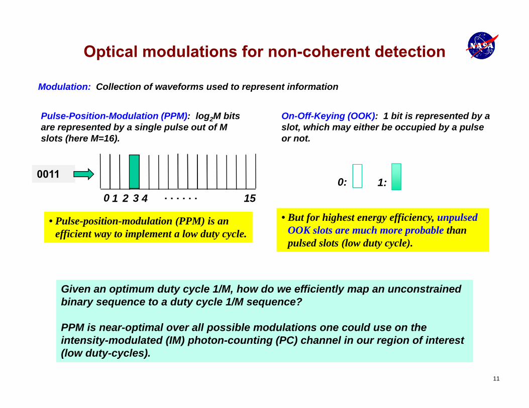
Pulse-Position-Modulation (PPM): log2M bits are represented by a single pulse out of M slots (here M=16).

On-Off-Keying (OOK): 1 bit is represented by a slot, which may either be occupied by a pulse or not.

0: 1:

Modulation: Collection of waveforms used to represent information

Optical modulations for non-coherent detection

Given an optimum duty cycle 1/M, how do we efficiently map an unconstrained binary sequence to a duty cycle 1/M sequence?

PPM is near-optimal over all possible modulations one could use on the intensity-modulated (IM) photon-counting (PC) channel in our region of interest (low duty-cycles).

• But for highest energy efficiency, unpulsedOOK slots are much more probable than pulsed slots (low duty cycle).

• Pulse-position-modulation (PPM) is an efficient way to implement a low duty cycle.

1212

Equivalent Channel model: Binary input, Poisson-distributed integer output

dark events

photon-counting photodetector

incident light

0:

1: Photon counts per slot

Synchronization

Intensity-modulated photon-counting channel model

Photo-electrons: Poisson point process

ns = mean signal photons per pulsed slotnb = mean background photons per slot

13

1 0 1 1 0 1 0 1 1 1 1

2 0 1 2 0 0 0 2 1 1 2

1 0 1 1 0 1 0

Modulation

Transmit symbols

Detect signal

Recover clock

Estimate data

Slotwidth

Detection

Ts

Synchronization

Receiving/Decoding

Fix data 1 0 1 1 0 1 0

0: 1:

Error-Correction-Coding (ECC)

Add parity

Form statistics

Signal processing steps to communicate the data

14

0 1 0 3 0 1 1 0

M=8

p(x=000|y) = 0.05p(x=001|y) = 0.2p(x=010|y) = 0.05p(x=011|y) = 0.3…

Capacity, hard and soft decisionsM = 16, Average power to achieve C = 1/8 bits/slot

1 2 3 4 5 6 7 8slot

count

Typical region of operation is between 0.01 and 1.0 photons/slot

Req

uire

d po

wer

to c

lose

link

(d

B p

hoto

ns/s

ymbo

l)

Noise photons/slot

Processing the photon counts: soft vs hard decisions

hard decision, erasing ties

15

Near-optimal signaling for a deep-space link

Mapping of the received signal power, noise power plane to optimum PPM orders

Slotwidth = 1.6 nsNo margin, no loss (assumes capacity achieving code)

As signal power increases, increase duty cycle, increasing the data rate

Typical Earth-Mars link would ideally use many PPM orders

over course of a Mars mission

1616

Fundamental capacity limitsIn this section, we discuss:• Fundamental capacity limits for ideal noiseless quantum

channel (i.e., only “quantum noise”).– Limits for given combinations of modulation and receiver.– The ultimate limit (Holevo capacity) for any quantum-consistent

measurement.• Capacity tradeoffs in terms of dimensional information

efficiency (DIE) vs photon information efficiency (PIE).– PIE is measured in bits/photon.– DIE is measured in bits/dimension, bits/sec/Hz per spatial mode.

• Alternative modulations/receivers to better approach the Holevo limit.

• Poisson model for noisy PPM or OOK channel capacity.

17

Asymptotic Holevo capacity limit

• Asymptotically, for large photon efficiency, the ultimate (Holevo) capacity efficiencies are related by:

• Thus, even at the ultimate limit, the dimensional efficiency (cd) must fall off exponentially with increasing photon efficiency (cp), except for a multiplicative factor proportional to cp.

cp = photon information efficiency (PIE) [bits/photon]

cd = dimensional information efficiency (DIE)

[bits/dimension] or[bits/s/Hz per spatial mode]

18

Asymptotic capacity of PPM and photon counting

• Asymptotically, for large photon efficiency, we have:

• Thus, with PPM and photon counting, and M optimized to achieve the best tradeoff, the dimensional information efficiency (cd) must fall off exponentially with increasing photon efficiency (cp).

• Comparing PPM + photon counting to the ultimate capacity, we obtain:

• Thus, the best possible factor by which the dimensional efficiency (cd) can be improved by replacing a conventional system with PPM and photon counting with one that reaches the ultimate Holevo limit is only linear in the photon efficiency (cp).

Can we approach Holevo capacity more

closely than PPM/OOK + photon counting?

1919

Dolinar receiver structure for BPSK or OOK

• The Dolinar receiver was extended to perform adaptive measurements on a coded sequence of binary coherent state symbols.

• There was no capacity improvement for the Dolinar receiver with adaptive priors.

feedback

+

Dolinar Receiver Soft-in Soft-out Decoder

updated priors

Enforce code constraints to

calculate updated symbol probabilities

measurements on symbolscoded symbols

• The Dolinar receiver is known to be the optimal hard-decision measurement on an arbitrary binary coherent-state alphabet.

• It is also an optimal soft-decision measurement (at least for BPSK) for maximizing the mutual information.

• Unfortunately, capacity improvements for OOK are minuscule relative to photon counting, and there’s still a brick-wall upper limit of 2 nats/photon for BPSK.

Dolinar receiverstructure

20

Fundamental free-space capacity limits vs state-of-the-art optical systems

0.00001

0.0001

0.001

0.01

0.1

1

10

100

0.00001

0.0001

0.001

0.01

0.1

1

10

100

0.001 0.01 0.1 1 10 100

Spec

tral

Effi

cien

cy p

er s

patia

l mod

e (b

its/s

ec/H

z pe

r spa

tial m

ode)

Dim

ensi

onal

Info

rmat

ion

Effic

ienc

y (b

its/m

ode)

Photon Information Efficiency (bits/photon)

ultimate quantum limit

BPSK+ultimate receiver

OOK+ultimate receiver

OOK+Dolinar receiver

OOK+photon counting

PPM+photon counting

BPSK+Dolinar receiver

coherent+homodyning

coherent+heterodyning

old demonstrated systems (JPL)

old demonstrated systems (LL)

new demonstrations (JPL 2012)

This is the ultimate quantum limit: Joint dimensional and photon efficiencies outside this curve (i.e., above and to the right) are unachievable.

Inferior curves represent theoretical limits with various constraints on the modulation and/or receiver.

Latest progress at JPL ( > 10 bits/photon)

21

Quantum-ideal number states:• EM-wave with deterministically

observable energy.• Propagation is degraded by

channel transmissivity (i.e., the probability transmitted number-state photon is not received at detector).

• With ideal transmissivity, number-states achieve Holevo limit (with Bose-Einstein priors).

• Binary number states are near-optimal at large bits/photon (with ideal transmissivity).

Channel given by Z-channel of coherent-state OOK with

Communicating with single-photon number states

Can we do (significantly) better than than PPM/OOK + photon counting?

Yes, using quantum number states instead of coherent states.

22

• Asymptotically at high PIE, OOK with single-photon number states achieves:

Asymptotic capacity of single-photon number states

For single-photon nunber states, the deviation from Holevo capacity is by a constant factor for a given channel, i.e., for a given transmissivity .

2323

Approximating number-state communicationusing coherent states with single-photon shutoff

• We can mimic the ideal photodetection statistics of the single-photon number state using receiver-to-transmitter feedback:

• The transmitter uses standard OOK or PPM modulation, and starts sending a coherent-state pulse every time the modulator calls for an “ON” signal.

• A standard photon-counting receiver is used.• Utilizing (ideal, instantaneous, costfree — i.e., very impractical) feedback from the

receiver, the transmitter turns off its pulse as soon as the first photon is detected.• If the transmitted pulse has very high intensity (“photon blasting”), this will ensure

that at least one (and therefore exactly one) photon will be detected, with very high probability.

• The feedback instructs the transmitter to stop sending wasted photons that carry no additional information.

symbol duration T

T

Turn off pulse at first photon detection

feedback

Pulse duration is min(,T)

Intensity of transmitted pulse (photons/s)

24

achieved at optimal value:

Asymptotic capacity of coherent states with single-photon shutoff

• Coherent-state OOK with single-photon shutoff economizes on photons by a factor d(), but expands bandwidth usage by the same factor d(), where is the pulse detection probability.

• This tradeoff is favorable at high PIE (and disadvantageous at high DIE).• The asymptotic capacity efficiency tradeoff is:

25

Coherent states with single-photon shutoff Single-photon number states

general @ opt. * general @ equiv. eq(*) @ opt. *

OOK0.274

@* = 0.876

0.274@

eq = 0.534

1.000@

* = 1

PPM0.150

@* = 0.715

0.150@

eq = 0.407

0.368@

* = 1

Summary of some Holevo capacity-approaching schemes

Table below shows the asymptotic ratio, at high PIE, of DIE for the specified scheme to the optimal Holevo DIE at the same PIE.

• is the non-erasure probability (detection probability) for the coherent state cases.• is the end-to-end efficiency for the number state cases.

26

Pi (Watts)

C (bits/sec) 2. Quantum-limited:

capacity linear in signal power

1.

1. Noise-limited: capacity quadratic in signal power

3. Bandwidth limited: saturation

2.

Blue: exactGreen: approx

Pn = noise powerE= energy per photon

3.

Poisson model for PPM channel capacity with noise• A Poisson channel model is used for

detection of signal in background noise.• The Poisson PPM channel capacity does

not, in general, have a closed form solution.• Approximations exist that provide insight into

its behavior.• The IM-PC channel has three regions as a

function of the signal power:1. Noise-limited: capacity is quadratic in

signal power.2. Quantum-limited: capacity is linear in

signal power.3. Band-width limited: capacity

saturates.• This differs from the coherent channel which

is linear or bandwidth limited.

Pi = minimum required power to close the link • Determined by inverting the capacity function at

the target data rate.• All other system components (receiver, decoder,

detector, etc.) are assumed to be ideal (no losses). M = PPM orderTs = slot width

2727

Coding to approach capacity

In this section, we discuss:• Choice of error correction code• Code inefficiency relative to capacity limit

28

Approaching capacity with an error correction code

wor

d er

ror r

ate

power efficiency (dB photons/bit)

Capacity, R

=1/2

• We signal utilizing a very power efficient error-correction code (ECC) that performs close to the capacity limit.

• With high probability, a codeword error will result if the signal power drops below the channel capacity.

• Pulse-Position-Modulation (PPM) contains memory, and may be considered part of the ECC.

• Iterative demodulation and decoding (of properly designed codes) provides gains of ~1.5 dB over non-iterative decoding.

• Codes designed explicitly for use with PPM provide gains over more general-purpose codes.

Capacity, R

=191/255

More power efficient

noise power = 86 dB p/s, Ts=0.5 ns

Error Correction Code

Modulatedata

Laser Transmitter Decode

De-Modulate

data

2929

Goal: Choose a code type that has near-capacity performance over all operating points, and low encoding/decoding complexity.

outer code(s) inner code

RSPPM Reed-Solomon (n,k)=(Ma-1), a=1[McEliece, 81], a>1 [Hamkins, Moision, 03]

PPM

PCPPM parallel concatenated convolutional [Kiasaleh, 98], [Hamkins, 99] (DTMRF, iterate with PPM [Peleg, Shamai, 00])

PPM

SCPPM convolutional [Massey, 81] (iterate with APPM) [Hamkins, Moision, 02]

(accumulate) PPM

LDPC-PPM low density parity check [Barsoum, 05] PPM

hard decisions

soft decisions

Some possible choices of code

30

• The most power efficient class of codes known for the noisy Poisson PPM channel are the serial concatenation of convolutional code with an accumulator and PPM (SCPPM)

• 3.3 -- 1.8 dB gain over baseline Reed-Solomon coded PPM (R=1/2)

• 0.4 dB gain over best known LDPC-coded PPM

• Complexity, performance favors SCPPM over LDPC-coded PPM

4-state (5,7) convolutional codeCRC used for

error detection and stopping rule

Operating point:(nb=0.2 photons/slot, M=64, Ts=32 nsec)

0.4 dB0.8 dB

LDPC code designed for BPSK channel

LDPC code designed for PPM channel

3.0 dB

Accumulate + PPM

Signal power (dB photons/slot)

Bit

Erro

r Rat

e

Example of SCPPM code architecture

3131

Bit

Err

or R

ate

Signal Photons/slot (dB)

Loss due to code inefficiency with respect to capacity

Capacity

Coding Gain=7.2 dB

Code Efficiency = 0.7 dB

• Measures of the error-control-code (ECC) performance:

1.Coding Gain = (code threshold) –(uncoded threshold)

2.Code Efficiency = (capacity threshold) – (code threshold)

• We use code efficiency code to measure ECC performance:• Provides an immediate measure of

additional gain that is possible by changing the code.

• For modern codes (LDPC, turbo), code efficiency is well characterized as constant over varying conditions, while error-rates do not have closed-form solutions.

Performance with ideal ECC

Performance with no ECC

ECC Performance

3232

Poisson-modeled noises

In this section, we discuss capacity limits with:• Thermal noise• Finite laser transmitter extinction ratio• Dark noise at the detector

33

Fundamental limit on capacity efficiency in noise

cp (bits/photon)

c d(b

its/d

imen

sion

)

NoiselessClassical (Shannon Capacity)

Channel described by input/output alphabets and probability map from input to output

Quantum (Holevo Capacity)Optimize Shannon capacity over all possible measurements (select probability map)

Characterize Efficiency:

cp = bits/photon (e.g., (bits/s)/Watt)cd = bits/dimension (e.g., (bits/s)/Hz)

Thermal Noisenb= 0.001 photons/mode

Noiseless Thermal Noise (conjectured)

34

• K background noise modes (white, Gaussian), N counts/mode

Noisy Poisson OOK channel for thermal noise

Poisson

Negative binomial

Poisson approximation to multimode thermal noise must become inaccurate at large cp for any number of noise modes. c d

(bits

/dim

ensi

on)

cp (bits/photon)

Holevo

1 noise photon/mode, 16 modes

10–5

10–10

10–0.5 10–0.2

• Photon information efficiency of Poisson OOK channel is unbounded

• Holevo limit (conjectured) is bounded

(nb = KN)

35

Noisy Poisson OOK channel for finite laser extinction ratio

• Finite transmitter extinction ratio generates a Poisson-distributed backgroundnoise proportional to the signal, nb = ns/.

• With finite extinction ratio , the photon efficiency of OOK + photon counting is strictly bounded:

P0= P1/= power transmitted in the off state

P1 = power transmitted in the on stateEffective signal photons

‘Signal’ photons appearing as noise

• Non-ideal transmitters transmit some power in the “OFF” state:• Power transmitted in the “OFF” state is proportional to power in the “ON” state; the

proportionality constant is the extinction ratio

3636

Dark noise at the photodetector• Photodetectors produce dark noise, which are

spurious photo-electrons that are present even with no incident light.

nb=0

6 bits/photon

nb =10.1 0.01

0.00110-4

10-5

10-6

10 bits/photon

• Noise levels with nb > 10-5 incur large losses at 10 bits/photon.

• Mitigation, by decreasing A and Ts, has limits

• A can only be decreased to the diffraction limit.

• Ts can only be decreased to bandwidth limit, and we will show that decreasing Ts also exacerbates other losses.

nb= ld A Ts dark e/slot

Device ld e/s/mm2)

Si GM-APD 106

InGaAsP GM-APD 108

NbN SNSPD 102

Dark rate

Active area

Slot-width

• Dark current generates a Poisson-distributed signal-independent background noise nb.

37

37Thus, achieving arbitrarily high cp on the noisy Poisson channel becomes impractical.

• With nonzero dark rate nb, the photon efficiency of OOK + photon counting is technically unbounded, but is effectively bounded, because cd drops off doubly-exponentially in a noisy Poisson channel.

• cd is approximately upper bounded by where• See the nearly vertical aqua curve, below its intersection with the noiseless Holevo bound

(where > 1). • This approximate bound crosses the noiseless OOK and Holevo curves at

• The actual cd breaks away sharply from thenoiseless OOK curve starting at a lower valueof cp, estimated empirically to be:

• This breakaway point can also be interpreted as:

Noisy Poisson OOK channel for detector dark noise

3838

Capacity limits with dark noise & finite extinction ratio

No dark noise Dark noise rate 10-6e/slot (e.g., 1 kHz dark rate, 1 ns slot)

44.5 dB extinction ratio

Ideal

44.5 dB extinction ratio

Ideal

• Each curve in these plots is the capacity efficiency tradeoff for a given PPM order M, and is generated by varying the average number of signal photons.

c d(b

its/d

imen

sion

)

c d(b

its/d

imen

sion

)

cp (bits/photon) cp (bits/photon)

3939

Other losses at the detector

In this section, we discuss:• Detector jitter• Photodetector blocking• Overall system engineering

4040

Detector jitter

Photon Counting Detector

ith Photon arrival at time ti …

…is detected at ti + random offset …

i

Measured hitter densities for some candidate detectors

Incident signal intensity

Jitter spreads the intensity

• Jitter is the random delay from the time a photon is incident on a photo-detector to the time a photo-electron is detected.

• Jitter losses are a function of the normalized jitter standard deviation:

• Thus, jitter limits our ability to decrease the slot width Ts without incurring loss.

jitter standard deviation

Slot-width

4141

Losses due to detector jitter

Knee at Ts = 0.1

dB L

oss

• Significant losses for Ts > 0.1• Effectively enforces a lower bound on Ts

• Limits data rate• Limits ability to mitigate dark noise

PPM

Ts=21

0.10.0

M=16, nb=1

Device ns

InGaAs(P) PMT 0.9

InGaAs(P) GM-APD 0.3

Si GM-APD 0.24

NbN SNSPD 0.03

Jitter Losses, Gaussian distributed

bits

/slo

t

42

Blocking

dark events

Ideal output: sequence of impulses at event times

Observed output

Ideal detector

Photo-detector may be modeled as an ideal detector followed by blocking

Blocking may be modeled via tracking of detector state with a Markov chain

Incident light intensity

= blocking duration

Photodetector blocking

• Certain photon-counting photodetectors are rendered inoperative (blocked) for some time (dead time) after each detection event

• 10—50 ns, Si GM-APD• 1—10 s, InGaAs GM-APD• 3—20 ns, NbN SNSPD Characterize impact of blocking by

= probability detector is unblocked

4343

Mitigating blocking= probability detector is unblocked

photon rate: decreased by temporal or spatial diffusion

11 l

Blocking may be mitigated by decreasing the peak incident photon rate (per detector)

• Temporally - Increase the slot-width and reduce the

photon rate, while preserving the photons/slot.

- Reduces impact of blocking, but lowers the date rate (bits/s), and integrates more noise

• Spatially- Increase Focal length, to decrease

signal intensity in the focal (detector) plane

- Integrates more noise

Ts 2Ts

F/D=8 F/D=16

We investigated this approach, numerically determining the optimum F number for a given blocking, dark noise, and target data rate (which fixes the aggregate required signal flux)

Make signal more diffuse in space

Make signal more diffuse in time

dead-time: fixed by the device

4444

Modeling blocking loss with arrayed detectors

Incident signal in background

Photon rates

Dark event rate

Blocking Approximate Model ( = 0)

= probability detector is unblocked

l=incident photon rate

Array output may be approximated as Poisson. Blocking attenuates the signal and noise.

Markov Model of Detector State

unblockedblocked

detection event

1

1 l

blocked capacity

unblocked capacity

Signal Power Loss: increase in power to achieve fixed capacity

u

b

CC

SNRlow

SNRhigh

ll

s

s

'

Capacity Loss: decrease in capacity at fixed signal power

4545

Parameter Blocking Jitter Dark Noise

F/D

Ts

M

• Mitigation of impairments results in conflicting demands on resources, hence requiring system engineering to optimize.

Mitigated by decreasing this parameter

Mitigated by increasing this parameter

Device requirements for high bits/photon operation

Non-ideality Requirement NbN SNSPD, Ts=1 ns

Extinction Ratio

> 60 dB presumed infinite for graph)

Jitter /Ts<0.1 0.03

Dark Noise ldTs<10-5 10-9

Blocking lp << 1.0 10-4

Losses due to dark noise, blocking and jitter. Optimized over F-number and duty cycle. Ts=1 ns, no background, 1-m aperture.

Overall system engineering considerations

4646

Atmospheric effects on optical communication

In this section, we discuss:• The effects of:

– Background radiation– Absorption/scattering– Clear sky turbulence effects– Pointing errors

• Fading channel models• Mitigating the effects of fading

47

• Background Radiation• Absorption/Scattering• Clear Sky Turbulence Effects

– Scintillation– Angle-of-Arrival Variations– Beam Spread– Beam Wander

Atmospheric effects on optical communication

[Piazzolla, ‘09]

48

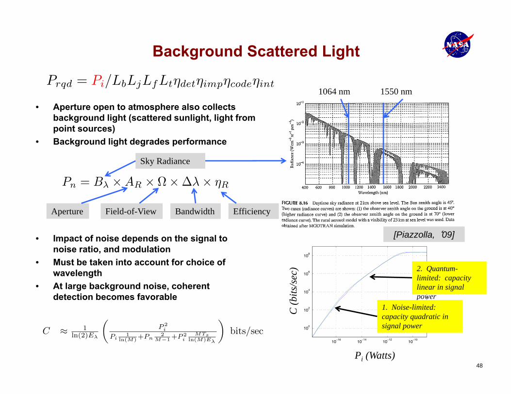
Background Scattered Light

• Aperture open to atmosphere also collects background light (scattered sunlight, light from point sources)

• Background light degrades performance

• Impact of noise depends on the signal to noise ratio, and modulation

• Must be taken into account for choice of wavelength

• At large background noise, coherent detection becomes favorable

Pi (Watts)

C (b

its/s

ec) 2. Quantum-

limited: capacity linear in signal power

1. Noise-limited: capacity quadratic in signal power

1064 nm 1550 nm

Sky Radiance

Aperture Field-of-View Bandwidth Efficiency

[Piazzolla, ‘09]

49

• Absorption and Scattering from aerosols (dust, etc.) and molecules (water vapor, etc.) attenuate the signal

• In bad weather (rain, snow, fog), attenuation can be severe, causing dropouts

• In Clear Sky, must budget for attenuation• Drives selection of bands with good clear

sky transmissivity• Candidates for Earth-Space link: 1064,

1550 nm • Typical attenuation for Space-Earth link

in near-infrared at zenith 0.1—0.3 dB• Outages at low elevation angles

Absorption/Scattering

1064 nm 1550 nm

[Piazzolla, ‘09]

50

• Random spatio-temporal mixing of air with different temperatures causes refractive-index variations

• Scintillation (constructive/destructive interference)

• Angle-of-arrival variations• Beam spreading• Beam wander

• Asymmetric Impacts:

Clear Sky Turbulence

Space-to-Earth:Angle-of-arrival (spatial distortion)Scintillation (fading)

Atmosphere (mostly concentrated in 0-20 km)

Earth-to-Space:Beam spread (attenuation)Beam wander (fading)

51

• Turbulence is a thin phase-screen in front of the transmitter aperture

• Coherence length is up to meters – Receiver always sees plane wave– Focused beam is diffraction-limited– Diffraction-limited spot moves in focal plane

• Beam-spread (attenuation)– Linear phase at transmitter tilts the beam– Higher-order phase spreads the beam (short-exposure < 1 msec)

• Beam-Wander → Scintillation – Irradiance fluctuates with log-normal distribution– Multiple transmit beams used to reduce scintillation

Beam Wander (Scintillation) & Beam Spread (Attenuation)

http://www.modulatedlight.org

Andrews & Phillips, Opt. Eng. (2006)

5252

• Random refractive index fluctuations also lead to phase distortions—constructive and destructive interference.

• Leads to Scintillation, random power fluctuations

• Each “coherence cell” has independent amplitude

– Aperture averaging: averaging over multiple coherence cells reduces the fluctuation in power (law of large numbers)

Temporal Distortions: Scintillation

0 0.5 1 1.5 2x 104

0

2

4

6

8

10

12

14

16

18

v(t)

t (msec)

Aperture

Pow

er

Measured fluctuations over a 45-km mountain-top to mountain-top link. [Biswas, Wright, ‘02]

Twinkling stars

5353

0 0.5 1 1.5 2x 104

0

2

4

6

8

10

12

14

16

18

v(t)

t (msec)

Pow

er

Time0 0.5 1 1.5 2 2.5 3 3.5 4

0

0.2

0.4

0.6

0.8

1

Random instantaneous power fluctuation in weak turbulence is well-modeled as log-normally distributed I

2 = scintillation index

Modeling scintillation: scintillation index

5454

Pow

er

Time

The power is highly correlated over short time intervals. The coherence time is the minimum duration over which two samples are (approximately) uncorrelated.

Coherence time goes as 1/band-width. 90% bandwidth is commonly used.

0 0.5 1 1.5 2x 104

0

2

4

6

8

10

12

14

16

18

v(t)

t (msec)

Typical coherence times are on the order of 10 msec

Tcoh = coherence time

Modeling scintillation: coherence time

55

4.2 4.25 4.3 4.35 4.40

0.2

0.4

0.6

0.8

1

1.2

1.4

1.6 Reduce fading to a two-parameter model:

Model fades as drawn independently from a log-normal distribution every Tcohseconds, and constant over those intervals.

Scintillation Index

Coherence Time

Nor

mal

ized

Po

wer

Time

Block fading model

56

• m=mean pointing error• =pointing error standard deviation• Gaussian beam, Gaussian pointing

erorrs

Losses due to dynamics similarly are linear in the variance

Fading due to pointing errors

[Barron, Boroson, ‘06]

57

4.2 4.25 4.3 4.35 4.40

0.2

0.4

0.6

0.8

1

1.2

1.4

1.6

Capacity Threshold

Time (s)

Nor

mal

ized

Pow

er

Codeword duration = 0.06 msec (at 125 Mbps data rate) << Tcoh

Loss due to outages ~5 dB in this example

Impact of fading on coded performance: outages

Average Signal Power (dB photons/slot)

Wor

d Er

ror R

ate

Capacity Threshold (no fading)

Performance (no fading)

Performance in fading

58

Rec

eive

d Po

wer

t (msec)

Time-varying received power

Interleaver

Capacity losses due to signal fadingR

ecei

ved

Pow

er

t (msec)

Fading capacity loss (unrecoverable)

Interleaving Efficiency (mitigated with interleaving)

• Nf = number of uncorrelated fades per codeword

• I2 scintillation index (variance of

normal in log-normal fading)

Cap

acity

thre

shol

d—no

fadi

ng

Cap

acity

thre

shol

d--f

adin

g

Cod

ewor

dE

rror

Rat

e

Signal Photons/Slot (dB)

59

Rec

eive

d Po

wer

t (msec)

Interleaver

Rec

eive

d Po

wer

t (msec)

Codeword duration = 0.06 msec

• Each codeword now sees N uncorrelated fades, or Powers

• Effectively transmitting over N parallel channels, each with a different power

• Relevant capacity is the instantaneous capacity, averaged over the N powers

C1(P1)

CN(PN)

Mitigating fading outages with interleaving

60

Fading Capacity Threshold

Fading Capacity: Fundamental limit on performance in fading.

Divide loss into two terms: int = finite interleaver loss (recoverable)2.Lf = Fading Capacity Loss (not recoverable)

Interleaving gain and fading capacity

N=124

8163

264128

256

Instantaneous capacity is a random variable

P(ou

tage

)

Fading capacity does not approach the capacity in the absence of fading. There is a loss due to fading dynamics, even with the same average received power.

The fading loss—the gap to the fading capacity, is nonrecoverable

Capacity Threshold (no fading)

Lf int

Signal Power (dB photons/slot)

61

Capacity function is, in general, not known in closed form

Linear approximation

dB Fading Capacity loss is linear in the scintillation index

Analytic approximation of fading capacity loss

0 0.1 0.2 0.3 0.4 0.50

0.5

1

1.5

2

2.5

approximation

Numerically evaluated loss

62

Fading loss = 0.5 dB (predicted 0.4)

Finite interleaver loss ~1.1 dB (predicted 1.2)

Analytic approximation of finite interleaver loss

Approximate as Gaussian for large N, and apply linear approximation

Interleaver Loss goes as the square root of the scintillation index

63

• Convolutional interleaver achieves same spreading (N) as a block interleaver with half the memory

• Example: to achieve N=100, with Tcoh=10 msec, Rb=125 Mbps, requires a 125 Mbit interleaver.

Interleaver memory requirements

B

2B

KB

shift registers

Laser Transmitter

B

2B

KB

Interleaver De-interleaver

Memory (bits)

Fades/codeword

Data Rate (bits/s)

Coherence Time (s)

6464

Conclusions• Free-space optical communication systems potentially gain

many dBs over RF systems.• There is no upper limit on the theoretically achievable photon

efficiency when the system is quantum-noise-limited:– Intensity modulations plus photon counting can achieve arbitrarily

high photon efficiency, but with sub-optimal spectral efficiency.– Quantum-ideal number states can achieve the ultimate capacity in

the limit of perfect transmissivity.• Appropriate error correction codes are needed to communicate

reliably near the capacity limits.• Poisson-modeled noises, detector losses, and atmospheric

effects must all be accounted for:– Theoretical models are used to analyze performance degradations.– Mitigation strategies derived from this analysis are applied to

minimize these degradations.