Fundamentals of Electromagnetics for Teaching and Learning: A Two-Week Intensive Course for Faculty...

Fundamentals of ElectromagneticsFundamentals of Electromagneticsfor Teaching and Learning:for Teaching and Learning:

A Two-Week Intensive Course for Faculty inA Two-Week Intensive Course for Faculty inElectrical-, Electronics-, Communication-, and Electrical-, Electronics-, Communication-, and

Computer- Related Engineering Departments in Computer- Related Engineering Departments in Engineering Colleges in IndiaEngineering Colleges in India

byby

Nannapaneni Narayana RaoNannapaneni Narayana RaoEdward C. Jordan Professor EmeritusEdward C. Jordan Professor Emeritus

of Electrical and Computer Engineeringof Electrical and Computer EngineeringUniversity of Illinois at Urbana-Champaign, USAUniversity of Illinois at Urbana-Champaign, USADistinguished Amrita Professor of EngineeringDistinguished Amrita Professor of Engineering

Amrita Vishwa Vidyapeetham, IndiaAmrita Vishwa Vidyapeetham, India

Program for Hyderabad Area and Andhra Pradesh FacultySponsored by IEEE Hyderabad Section, IETE Hyderabad

Center, and Vasavi College of EngineeringIETE Conference Hall, Osmania University Campus

Hyderabad, Andhra PradeshJune 3 – June 11, 2009

Workshop for Master Trainer Faculty Sponsored byIUCEE (Indo-US Coalition for Engineering Education)

Infosys Campus, Mysore, KarnatakaJune 22 – July 3, 2009

6-3

Module 6Statics, Quasistatics, and

Transmission Lines6.1 Gradient and electric potential6.2 Poisson’s and Laplace’s equations6.3 Static fields and circuit elements6.4 Low-frequency behavior via quasistatics6.5 Condition for the validity of the quasistatic approximation6.6 The distributed circuit concept and the transmission-line

6-4

Instructional Objectives42. Understand the geometrical significance of the gradient operation43. Find the static electric potential due to a specified charge distribution by applying superposition in conjunction with the potential due to a point charge, and further find the electric field from the potential44. Obtain the solution for the potential between two conductors held at specified potentials, for one- dimensional cases (and the region between which is filled with a dielectric of uniform or nonuniform permittivity, or with multiple dielectrics) by using the Laplace’s equation in one dimension, and further find the capacitance per unit area (Cartesian) or per unit length (cylindrical) or capacitance (spherical) of the arrangement

6-5

Instructional Objectives (Continued)

45. Perform static field analysis of arrangements consisting of two parallel plane conductors for electrostatic, magnetostatic, and electromagnetostatic fields46. Perform quasistatic field analysis of arrangements consisting of two parallel plane conductors for electroquastatic and magnetoquasistatic fields47. Understand the condition for the validity of the quasistatic approximation and the input behavior of a physical structure for frequencies beyond the quasistatic approximation 48. Understand the development of the transmission-line (distributed equivalent circuit) from the field solutions for a given physical structure and obtain the transmission- line parameters for a line of arbitrary cross section by using the field mapping technique

6.1 Gradient and Electric Potential

(EEE, Secs. 5.1, 5.2; FEME, Sec. 6.1)

6-7

Gradient and the Potential Functions

0

x y z

x y z

x y z

x y z

x y zA A A

x y z

x y z

x y zA A A

a a a

× A

× A × A × A × A

6-86-8

Since 0,B

B can be expressed as the curl of a vector.

Thus

A is known as the magnetic vector potential.

B = × A

Then

t

t

× E = × A

A×

6-9

t

AE +

is known as the electric scalar potential.

0t

A× E +

t

AE =

is the gradient of

x y z

x y z

x y z

x y z

a a + a

a a a

6-10

0

x y z

x y z

x y z

x y z

x y z

x y z

a a a

×

a a a

6-116-11

Basic definition of :

d d l

, ,P x y z

, ,Q x dx y dy z dz

x y z x y zd dx dy dzx y z

d

a a a a a a

l

For a constant surface, d = 0. Therefore is normal to the surface.

P

6-126-12

cos

cos

n

nd d

dl

d d

dl dn

a

a l

Thus, the magnitude of at any point P is the rate of increaseof normal to the surface, which is the maximum rate of increase at that point. Thus

n

d

dn

a

Useful for finding unit normal vector to the surface.

d l

0 =

QP

dn

0 d =

na

6-136-13

D5.1 Finding unit normal vectors to the surface

2 2 2, , 2 2x y z x y z

2 2 22 2 8x y z at several points:

2 2 2

2 2 2

2 2 2

2 2

2 2

2 2

4 4 2

x

y

z

x y z

x y zx

x y zy

x y zzx y z

a

a

a

a a a

6-146-146-14

( ) At 2, 2, 0 ,a

4 2 4 2

24 2 4 2

x y x yn

x y

a a a aa

a a

( ) At 1,1, 2 ,b

4 4 4

4 4 4 3x y z x y z

n

x y z

a a a a a aa

a a a

( ) At 1, 2, 2 ,c

4 4 2 2 2 2 2

74 4 2 2 2

x y z x y zn

x y z

a a a a a aa

a a a

6-156-15

t

B

× E =

t

B = 0

B = × A

AE =

t

D

× H = J +

D =

(1)

(2)

(4)

(4)

(3)

(1)

2

t

t

A

A

(3)

6-166-16

Using , we obtaint

A =

22

2t A

A J

22

2t

Potential function equations

2

22

1t t

t t

AA J

AA A J

(2)

6-17

Laplacian of scalar

Laplacian of vector

In Cartesian coordinates,

2

2 A = A × × A

2 2 22

2 2 2x y z

2 2 2 2x x y y z zA A A A = a a a

6-186-18

B B

A A

B A

BA

A B

d d

d

E

E l l

also known as the potential difference between A andB, for the static case.

Voltage between and

B

A BAd V V

A B

E lBut,

For static fields, 0,t

6-19

Given the charge distribution, find V using superposition.Then find E using the above.

V VE

since

agrees with the previously known result.

For a point charge at the origin,

4

QV

r

2

4

4

r

r

r

VV

r

Q

r r

Q

r

E a

a

a

6-20

Thus for a point charge at an arbitrary location P

Q

R

P

P5.9

4

QV

R

r

z

a 2

1

a

z

dz

6-21

Considering the element of length dz at (0, 0, z), we have

Using

0

224

L dzdV

r z z

tan z z r 2 secd z r d

20

0

sec

4 sec

sec4

L

L

r ddV

r

d

6-226-22

for z a

1

2

1

2

0

0

0 2 2

1 1

2

0

2

sec 4

1n sec tan 4

sec tan 1n

4 sec tan

1n4

a

z a

L

L

L

2

L

2

V dV

d

r z a z a

r z a z a

6-23

Magnetic vector potential due to a current element

R

P

I d l4

I d

R

l

A

Analogous to

4

QV

R

6-24

Review Questions6.1. What is the divergence of the curl of a vector?6.2. What is the expansion for the gradient of a scalar in Cartesian coordinates? When can a vector be expressed as the gradient of a scalar?6.3. Discuss the basic definition of the gradient of a scalar.6.4. Discuss the application of the gradient concept for the determination of unit vector normal to a surface.6.5. Define electric potential. What is its relationship to the electric field intensity?6.6. Distinguish between voltage as applied to time-varying fields and potential difference.6.7. What is the electric potential due to a point charge? Discuss the determination of electric potential due to a charge distribution.

6-25

Review Questions (Continued)6.8. What is the Laplacian of a scalar? What is the expansion for the Laplacian of a scalar in Cartesian coordinates?6.9. What is the magnetic vector potential? How is it related to the magnetic flux density?

6-26

Problem S6.1. Finding the gradient of a two-dimensional function and associated discussion

6-27

Problem S6.2. Finding the angle between two plane surfaces, by using the gradient concept

6-28

Problem S6.3. Finding the image charge(s) for a point charge in the presence of a conductor

6-29

Problem S6.3. Finding the image charge(s) for a point charge in the presence of a conductor (Continued)

6.2 Poisson’s and Laplace’s Equations

(EEE, Sec. 5.3; FEME, Sec. 6.2)

6-31Poisson’s Equation

For static electric field,

Then from

If is uniform,

D =

Poisson’s equation

0t

B

× E =

VE =

V

V

V

V

6-32If is nonuniform, then using

Thus

Assuming uniform , we have

For the one-dimensional case of V(x),

,

V V V

V V

V V

2 2 2

2 2 2

V V V

x y z

2

2

V

x

6-33

Anode, x = d V = V0

Cathode, x = 0 V = 0

Vacuum Diode

D5.7

(a) 8x dV

4 3 4 3

0 0 1 2

00 2 3

1 1

88

1

8 4

V V

VV

4 3

0

xV V

d

6-34

(b) 8 8

8

1 3

0

8

1 3

0

0

4

3

4 1

3 8

2

3

d d

xd

x

d

x

x

x x

x

x

V

V

x

V x

d d

V

d

V

d

E

a

a

a

a

6-35

(c)

8 0 8

2

0 2

8

2 3

00 2

8

2 3

00 2

2 300 2

0 02

4

9

4 1

9 8

48

916

9

d d

d

d

x x

x

x

V

V

x

V x

d d

V

d

V

dV

d

6-366-36Laplace’s Equation

Let us consider uniform first.

E6.1. Parallel-plate capacitor

If Poisson’s equation becomes

x = d, V= V0

x = 0, V = 0

0 for uniform V

0 for nonuniform V V

6-37

Neglecting fringing of field at edges,

General solution

V V x

2

20

VV

x

VA

x

V Ax B

6-38Boundary conditions

Particular solution

0

00

0 at 0

at

0 0 0

0

V x

V V x d

B B

VV Ad A

d

0

x

x

VV

xV

d

E a

a

0VV x

d

6-39

x = d

x = 0

xa

xx a

0

0

0

0

0

for 0

for

for 0

for

for 0

for

x xS n

x x d

x x

x x

x

x d

Vx

dV

x dd

Vx

dV

x dd

a Ea D

a E

a a

a a

6-40

area of plates

For nonuniform

For

0

0

SQ A

V A

dQ A

CV d

2 0V V

,V V x2

20

V V

x x x

0V

x x

6-41

E6.2

x = d, V = V0

x = 0, V = 0

0 12

x

d

0 1 02

1 02

x V

x d x

x V

x d x

12

x VA

d x

6-42

21 xd

V A

x

0 for 0V x

0 for V V x d

2 1n 12

xV Ad B

d

0 2 1n 1 0Ad B B

00 3

2

32 1n

2 2 1n

VV Ad A

d

0 1n 11n 1.5 2

V xV

d

6-43

0

2

1

2 1n 1.5 1

x

xxd

VV

xV

d

Ε a

a

0 0

0 00

0 0

0

0

0

2 1n 1.5

2 1n 1.5

2 1n 1.5

2 1n 1.5

2 1n 1.5

x

S Sx x d

S

V

d

V

d

V AQ A

d

AQC

V d

C

A d

D Ε = a

6-44

Review Questions6.10. State Poisson’s equation for the electric potential. How is it derived?6.11. Outline the solution of the Poisson’s equation for the potential in a region of known charge density varying in one dimension.6.12. State Laplace’s equation for the electric potential. In what regions is it valid?6.13. Outline the solution of Laplace’s equation in one dimension by considering a parallel-plate arrangement.6.14. Outline the steps in the determination of the capacitance of a parallel-plate capacitor.

6-45

Problem S6.4. Solution of Poisson’s equation for a space charge distribution in Cartesian coordinates

6-46

Problem S6.5. Finding the capacitance of a spherical capacitor with a dielectric of nonuniform permittivity

6.3 Static Fields and Circuit Elements


6-486-48

Classification of Fields

Static Fields ( No time variation; ) Static electric, or electrostatic fields

Static magnetic, or magnetostatic fieldsElectromagnetostatic fields

Dynamic Fields (Time-varying)

Quasistatic Fields (Dynamic fields that can be analyzed as though the fields are static) Electroquasistatic fields Magnetoquasistatic fields

0t

6-496-496-49

Static Fields

For static fields, , and the equations reduce to

D =

B 0

J 0

E d l0C

HdlC JdS

SDdS dv

VSB dS 0

SJdS 0

S

0t

0 ×E

× H J

6-506-50

Solution for charge distribution

Solution for point charge

Electric field dueto point charge

Solution for Potential and Field

1 ( )( )

4 V

V dv

r

rr r

( )( )

4

QV

rr

r r

E(r) Q( r )(r r )

4 r r 3

6-516-51

Laplace’s Equation and One-Dimensional Solution

2

20

d V

dx

Laplace’s equation

For Poission’s equation reduces to

Ax + B

2 0V

6-526-52

Example of Parallel-Plate Arrangement:Capacitance

0( ) ( )V

V x d xd

S

S

(b)

y

z

x

(a)

x

y z

w

x= 0

x = d

l

z – l

d

z z = 0

V0

z = – l z = 0z

––

– – – – – –

E, DV0

x 0, V =V0

x d, V = 0

6-536-53

D V0

dax

00( )

V wlQ wl V

d d

C QV0

wld

0x

VV

d E a

We 12

Ex2

(wld) 1

2wld

V0

2 12

CV02

Capacitance of the arrangement, F

Electrostatic Analysis of Parallel-Plate Arrangement

C w ld

6-546-54

Magnetostatic Fields

Poisson’s equation formagnetic vector potential

2A –J

B 0

Hdl JdSSC

BdS 0S

× H J

6-556-55

Solution for current distribution

Solution for current element

Magnetic field dueto current element

( )( )

4 V

dv

J r

A rr r

( )( )

4

I d

l r

A rr r

2A = 0 For current-free region

Solution for Vector Potential and Field

3

4

I d

l r × r rB r

r r

6-566-56

Example of Parallel-Plate Arrangement:Inductance

(b)x

y zx = 0

x d

z – l z = 0z

H, BI0

JS

(a)

y

z

xx = 0

x = d

z – l z = 0

l

w d

z

I0

6-576-57

0 0 0

x y z

x y z

xH H H

a a a Bxx

0

H I0w

ay

Magnetostatic Analysis of Parallel-Plate Arrangement

JS (I0 w)az on the plate x 0

(I0 w)ax on the plate z 0

(I0 w)az on the plate x d

6-58

B I0w

ay

I0w

(dl) dl

w

I0

L I0

dlw

Wm 12

H2

(wld) 1

2dlw

I0

2 12

LI02

Inductance of the arrangement, H

Magnetostatic Analysis of Parallel-Plate Arrangement (Continued)

L dlw

6-59

Electromagnetostatic Fields

D 0

B 0

(J Jc E)

Edl0C

HdlC JcdS

S EdSS

DdS 0S

BdS 0S

x E 0

x H Jc E

6-606-60

Example of Parallel-Plate Arrangement

(b)

(a)

y

z

x

x

y z

w

x = 0

x = d

l

z – l

d

z z = 0

V0

z = – l z = 0z

x d, V 0

––

– – – – – –

H, BDE,V0

Ic

x 0, V V0

Jc ,

JS

JS

S

SS

S

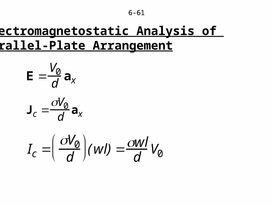
6-616-61

E V0d

ax

Jc V0

dax

Ic V0d

(wl) wl

dV0

Electromagnetostatic Analysis of Parallel-Plate Arrangement

6-62

G IcV0

wld

R V0Ic

dwl

Pd (E2 )(wld) wld

V0

2

GV02

V02

R

Conductance, S

Resistance, ohms

Electromagnetostatic Analysis of Parallel-Plate Arrangement (Continued)

6-636-63

0yH V

z d

Internal Inductance


Li 1Ic

N d z l

0

H V0

dz ay

13

dlw

H Hy(z)ay

Hyd(dz 1Ic

– z l

z –l

0

6-64


V0

R d wl

Li 13

dlw

C wld

Equivalent Circuit

Alternatively, from energy considerations,

Li 1Ic

2 (dw ) Hy2

dzzl

0

13

dlw

6-65

Review Questions6.15. Discuss the classification of fields as static, dynamic, and quasistatic fields.6.16. State Maxwell’s equations for static fields in (a) integral form, and (b) differential form.6.17. Outline the steps involved in the electrostatic field analysis of a parallel-plate structure and the determination of its capacitance.6.18. Outline the steps involved in the magnetostatic field analysis of a parallel-plate structure and the determination of its inductance.6.19. Outline the steps involved in the electromagnetostatic field analysis of a parallel-plate structure and the determination of its circuit equivalent.6.20. Explain the term, “internal inductance.”

6-66

Problem S6.6. Finding the internal inductance per unit length of a cylindrical conductor arrangement

6.4 Low Frequency Behaviorvia Quasistatics


6-68

Quasistatic Fields

For quasistatic fields, certain features can be analyzed as though the fields were static. In terms of behavior in the frequency domain, they are low-frequency extensions of static fields present in a physical structure, when the frequency of the source driving the structure is zero, or low-frequency approximations of time-varyingfields in the structure that are complete solutions to Maxwell’s equations. Here, we use the approach of low-frequency extensions of static fields. Thus, for a given structure, we begin with a time-varying field having the same spatial characteristics as that of the static field solution for the structure and obtain field solutions containing terms up to and including the first power (which is thelowest power) in for their amplitudes.

6-69

Electroquasistatic Fields

Vg t V0 cos t

x

y z

z = –l z = 0z–

– – –

Ig (t)

+–

x 0

x d

– – – –

H1

E0

JS

S

6-706-70

1 0 0 siny xH D V

tz t d

Electroquasistatic Analysis of Parallel-Plate Arrangement

E0 V0

dcos t ax

H1 V0z

dsin t ay

6-71

whereI g j CV g C wld

Electroquasistatic Analysis of Parallel-Plate Arrangement (Continued)

C w ld

Ig (t)w Hy1 z l

wld

V0 sin t

CdVg (t)

dt

6-72

Electroquasistatic Analysis of Parallel-Plate Arrangement (Continued)

Pin wd Ex0 Hy1 z0

wld

V0

2sin t cos t

ddt

12

CVg2

6-73

Magnetoquasistatic Fields

x

y zx = 0

x d

z – l z = 0z

– – – – –

–Vg (t)

E1

H0

JS

Ig t I0 cos t

S

6-746-74

01 0 sinyxBE I

tz t w

Magnetoquasistatic Analysis of Parallel-Plate Arrangement

H0 I0w

cos t ay

E1 I0z

wsin t ax

6-75

V g jL I g where

Magnetoquasistatic Analysis of Parallel-Plate Arrangement (Continued)

L dlw

L dlw

Vg (t) d Ex1 z l

dlw

I0 sin t

LdIg(t)

dt

6-76

Magnetoquasistatic Analysis of Parallel-Plate Arrangement (Continued)

Pin wd Ex1Hy0 z l

dlw

I0

2sin t cos t

ddt

12

LIg2

6-77

Quasistatic Fields in a Conductor

(b)

(a)

(c)

x

y z

z = –l z z = 0

Ex1

z = –l z z = 0

Hy 0

Ex 0

z = –l z = 0z

x 0

x d

+–

IgH0E0, J c0

Hyd1 Hyc1

Vg t V0 cos t

6-786-78

01 0 sinyxBE V z

tz t d

2 201 sin

2x

VE z l t

d

Quasistatic Analysis of Parallel-Plate Arrangement with Conductor

Jc0 E0 V0

dcos t ax

E0 V0d

cos t ax

H0 V0z

dcos t ay

6-796-79

2 3 20 0

1

3sin sin

6y

V z zl V zH t t

d d

Quasistatic Analysis of Parallel-Plate Arrangement with Conductor (Continued)

1 01

22 20 0sin sin

2

y xx

H EE

z t

V Vz l t t

d d

6-80

E x V gd

j 2d

z2 l2 V g

H y zd

V g j zd

V g j 2 z3 3zl2

6dV g

Hy V0 z

dcos t

V0 zd

sin t 2V0 z3 3zl2

6dsin t


Ex V0

dcos t

V0

2dz

2 l2 sin t

6-81


Y in I gV g

j wld

wld

1 j l2

3

j wld

1d

wl 1 j l2

3

I g w H y z l

wld

j wld

j 2wl

3

3d

V g

6-826-82

Equivalent Circuit

Y in j wld

1d

wl j dl3w

j C 1R jLi

V0 C wld

R d wl

Li 13

dlw


6-83

Review Questions6.21. What is meant by the quasistatic extension of the static field in a physical structure?6.22. Outline the steps involved in the electroquasistatic field analysis of a parallel-plate structure and the determination of its input behavior. Compare the input behavior with the electrostatic case.6.23. Outline the steps involved in the magnetoquasistatic field analysis of a parallel-plate structure and the determination of its input behavior. Compare the input behavior with the magnetostatic case.6.24. Outline the steps involved in the quasistatic field analysis of a parallel-plate structure with a conducting slab between the plates and the determination of its input behavior. Compare the input behavior with the electromagnetostatic case.

6-84

Problem S6.7. Frequency behavior of a capacitor beyond the quasistatic approximation

6-85

Problem S6.7. Frequency behavior of a capacitor beyond the quasistatic approximation (Continued)

6-86

6.5 Condition for the validity ofthe quasistatic approximation (EEE, Sec. 5.5; FEME, Secs. 6.5, 7.1)

6-87

We have seen that quasistatic field analysis of a physical structure provides information concerning the low-frequency input behaviorof the structure. As the frequency is increased beyond that for which the quasistatic approximation is valid, terms in the infinite series solutions for the fields beyond the first-order terms need to be included. While one can obtain equivalent circuits for frequencies beyond the range of validity of the quasistatic approximation by evaluating the higher order terms, we shall here obtain the exact solution by resorting to simultaneous solution of Maxwell’s equations to find the condition for the validity of thequasistatic approximation, and further investigate the behavior for frequencies beyond the quasistatic approximation. We shall do this by considering the parallel-plate structure, and obtaining the wavesolutions, which will then lead us to the distributed circuit concept and the transmission-line.

6-886-88

Wave Equation

One-dimensional wave equation

For the one-dimensional case of

E Ex z, t ax and H = Hy z, t ay ,

t t

B H

×Et t

D E

× H

yxHE

z t

y x

H E

z t

2 2

2 2x xE E

z t

6-896-89

Solution to the One-Dimensional Wave Equation

Traveling wave propagating in the +z direction

–1

1 t 0

0z

1 2 f

1 f

t 4 t

2

( , ) cos cosxE z t A t z B t z

cos t z

6-906-90

Solution to the One-Dimensional Wave Equation

Traveling wave propagating in the –z direction

t 2

t 01

–1

0–z

1 2 f

1 f

1( , ) cos cosyH z t A t z B t z

t 4

cos t z

6-916-91

E x A e j z B e j z

H y 1 A e jz B e j z

Phase constant

Phase velocity

Intrinsic impedance

pv

General Solution in Phasor Form

1vp

A Ae j

, B Be j –

,

,

,

6-926-92

s

Vg t V0 cos t

Example of Parallel-Plate StructureOpen-Circuited at the Far End

E x V g

d cos lcos z H y

jV gd cos l

sin z

H y 0 at z = 0

E x V gd

at z =l

B.C.

x

y z

z = –l z = 0z

–

– – –

Ig (t)

+–

x 0

x d

– – – –

JS

E

HS

6-93

Standing Wave Patterns (Complete Standing Waves)

72

0–z

Hy

0–z

Ex

52

32

2

3

2

6-94

Complete Standing Waves

Complete standing waves are characterized by pure half-sinusoidal variations for the amplitudes of the fields. For values of z at which the electric field amplitude is a maximum, the magnetic field amplitude is zero, and for values of z at which the electric field amplitude is zero, the magnetic field amplitude is a maximum. The fields are also out of phase in time, such that at any value of z, the magnetic field and the electric field differ in phase by t = / 2.

6-95

Input Admittance

For l << 1,

Y in I gV g

j wd

tan l

Y in jwd

(l)

j wld

wld

I g w H y z l

jwV g d

tan l

Y in j w

dl (l)

3

3 2(l)

5

15

6-96

Condition for the Validity of the Quasistatic ApproximationThe condition l << 1 dictates the range of validity for the quasistatic approximation for the input behavior of the structure. In terms of the frequency f of the source, this condition means that f << vp/2l, or in terms of the period

T = 1/f, it means that T >> 2(l/vp). Thus, quasistatic fields are low-frequency

approximations of time-varying fields that are complete solutions to Maxwell’s equations, which represent wave propagation phenomena and can be approximated to the quasistatic character only when the times of interest are much greater than the propagation time, l/vp, corresponding to the length of the

structure. In terms of space variations of the fields at a fixed time, the wavelength ( = 2 ), which is the distance between two consecutive points along the direction of propagation between which the phase difference is 2, must be such that l << /2 ; thus, the physical length of the structure must be a small fraction of the wavelength.

6-976-97

For frequencies slightly beyond the approximation l <<1,

Y in j wd

l (l)3

3

j wld

1 wl

d

dl

3w

1

13

1( ) 3

Zwl wl dl

jd d w

dlj

j wl d w

in

wld

13

dlw

6-98

In general, tan l

f

3vp

4l

5vp

4l0 vp

2l

vp

l3vp

2l

vp

4 l

Yin

Yin

capacitive

inductive

6-99

E x jI g

w cos lsin z H y

I gw cos l

cos z

s

Ig t I0 cos t

Example of Parallel-Plate StructureShort-Circuited at the Far End

x

y zx = 0

x d

z – l z = 0z

– – – – –

–Vg (t)

JS

E

H

E x 0 at z 0

H y I gw

at z l

B.C.

6-100

Standing Wave Patterns (Complete Standing Waves)

0–z

Hy

0–z

Ex

3

2

72

52

32

2

6-101

Input Impedance

For l << 1,

Z in V gI g

jdw

tan l

Z in dw

(l)

j dlw

dlw

Z in j

dw

l ( l)3

3 2( l)

5

15

V g d E x z l

j dI g

wtan l

6-102

For frequencies slightly beyond the approximation l <<1,

Z in jdw

l ( l)3

3

j dlw

1 dl

w

wl

3d

Y in 1

j dlw

1 dl

w

wl

3d

1j (dl / w)

j wl3d

13

wld

dlw

6-103

In general,

tan l

3vp

4 l5vp

4l0 vp

2 l

vp

l3vp

2 l

vp

4 l

capacitive

inductive

Zin

Zin

f

6-104

Review Questions6.25. Outline the steps in the solution for the electromagnetic field in a parallel-plate structure open-circuited at the far end. 6.26. What are complete standing waves? Discuss their characteristics.6.27. What is the input admittance of a a parallel-plate structure open-circuited at the far end? Discuss its variation with frequency.6.28. State and discuss the condition for the validity of the quasistatic approximation.6.29. Outline the steps in the solution for the electromagnetic field in a parallel-plate structure short-circuited at the far end. 6.30. What is the input impedance of a a parallel-plate structure short-circuited at the far end? Discuss its variation with frequency.

6-105

Problem S6.8. Frequency behavior of a parallel-plate structure from input impedance considerations

6-106

Problem S6.8. Frequency behavior of a parallel-plate structure from input impedance considerations (Continued)

6.6 The Distributed Circuit Concept and the Transmission Line

(EEE, Secs. 6.1, 11.5; FEME, Secs. 6.5, 6.6)

6-134

Review Questions6.31. Discuss the phenomenon taking place in a parallel-plate structure at any arbitrary frequency.6.32. How is the voltage between the two conductors in a given cross-sectional plane of a parallel-plate transmission line related to the electric field in that plane?6.33. How is the current flowing on the plates across a given cross-sectional plane of a parallel-plate transmission line related to the magnetic field in that plane?6.35. Discuss transverse electromagnetic waves.6.36. What are transmission-line equations? How are they derived from Maxwell’s equations?

6-135

Review Questions6.37. Discuss the concept of the distributed equivalent circuit. How is it obtained from the transmission-line equations?6.38. Discuss the solutions for the transmission-line equations for the voltage and current along a line.6.39. Explain the “characteristic impedance” of a transmission line.6.40. Discuss the relationship between the transmission-line parameters.6.41. What are the transmission-line parameters for a parallel- plate line?6.42. Describe the curvilinear squares technique of finding the line parameters for a line with an arbitrary cross section.

6-136

Problem S6.9. Transmission-line equations and power flow from the geometry of a coaxial cable

6-137

Problem S6.10. Application of the curvilinear squares technique for an eccentric coaxial cable

The End

Fundamentals of Electromagnetics for Teaching and Learning: A Two-Week Intensive Course for Faculty...

Documents

Transcript of Fundamentals of Electromagnetics for Teaching and Learning: A Two-Week Intensive Course for Faculty...