Fundamentals of Digital Audio

The Central Problem

Waves in nature, including sound waves, are continuous:

Between any two points on the curve, no matter how close together they are, there are an infinite number of points

The Central Problem

Analog audio (vinyl, tape, analog synths, etc.) involves the creation or imitation of a continuous wave.

Computers cannot represent continuity (or infinity).

Computers can only deal with discrete values. Digital technology is based on converting

continuous values to discrete values.

Digital Conversion

The instantaneous amplitude of a continuous wave is measured (sampled) regularly. The measurement values, samples, may be stored in a digital system.

This encoding format is called pulse code modulation, or PCM

Digital Conversion

The instantaneous amplitude of a continuous wave is measured (sampled) regularly. The measurement values, samples, may be stored in a digital system.

0.9925

0.9945

0.9961

0.99750.9986

0.99930.9998 1.0

0.99980.9993

0.99860.9975

0.9961

0.9945

0.9925

Digital Conversion

The instantaneous amplitude of a continuous wave is measured (sampled) regularly. The measurement values, samples, may be stored in a digital system.

[ 0.9925, 0.9945, 0.9961, 0.9975, 0.9986, 0.9993, 0.9998, 1.0, 0.9998, 0.9993, 0.9986, 0.9975, 0.9961, 0.9945, 0.9925 ]

Digital Audio

Digital representation of audio is analogous to cinema representation of motion.

We know that “moving pictures” are not really moving; cinema is simply a series of pictures of motion, sampled and projected fast enough that the effect is that of apparent motion.

With digital audio, if a sound is sampled often enough, the effect is apparent continuity when the samples are played back.

Digital Audio

Con:– It is, at best, only an approximation of the wave

Pros:– Significantly lower background noise levels– Sounds are more reliably stored and duplicated– Sounds are easier to manipulate:

Rather than worry about how to change the shape of a wave, engineers need only perform appropriate numerical operations

Digital Audio

The theory behind digital representation has existed since the 1920s.

It wasn’t until the 1950s that technology caught up to the theory, and it was possible to implement digital audio.

Digital Audio

Bell Labs produced the first digital audio synthesis in the 1950s.

For computer synthesis, a series of samples was calculated and stored in a wavetable.

Reading through the wavetable at different rates (skipping every n samples, the sampling increment) allowed different pitches to be created.

Audio was produced by feeding the samples that were to be audified through a digital to analog converter (DAC).

Digital Audio

Contemporary computer sound cards often contain a set of wavetable sounds.

The function is the same: a library of samples describing different waveforms.

Digital Audio

Digital recording became possible in the 1970s.

Voltage input from a microphone is fed to an analog to digital converter (ADC), which stores the signal as a series of samples.

The samples can then be sent through a DAC for playback.

Digital Audio

Thus, the ADC produces a “dehydrated” version of the audio.

The DAC then “rehydrates” the audio for playback.

(Gareth Loy, Musimathics v. 2)

Characteristics of Digital Audio

With digital audio, we are concerned with two measurements:– Sampling rate– Quantization

With these measurements, we can describe how well a digitized audio file represents the analog original.

Sampling Rate

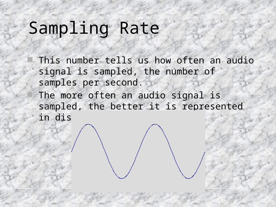
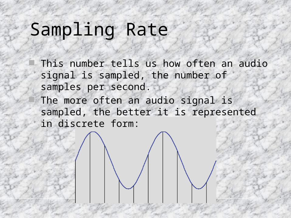
This number tells us how often an audio signal is sampled, the number of samples per second.

The more often an audio signal is sampled, the better it is represented in discrete form:

Sampling Rate

This number tells us how often an audio signal is sampled, the number of samples per second.

The more often an audio signal is sampled, the better it is represented in discrete form:

Sampling Rate

This number tells us how often an audio signal is sampled, the number of samples per second.

The more often an audio signal is sampled, the better it is represented in discrete form:

Sampling Rate

This number tells us how often an audio signal is sampled, the number of samples per second.

The more often an audio signal is sampled, the better it is represented in discrete form:

Sampling Rate

This number tells us how often an audio signal is sampled, the number of samples per second.

The more often an audio signal is sampled, the better it is represented in discrete form:

Sampling Rate

This number tells us how often an audio signal is sampled, the number of samples per second.

The more often an audio signal is sampled, the better it is represented in discrete form:

Of course, this staircase-shaped wave needs to be smoothed.

This process will be covered during the discussion on filtering.

Sampling Rate

So we want to sample an audio wave every so often.The question is: how “often” is “often enough”?

Harry Nyquist of Bell Labs addressed this question in a 1925 paper concerning telegraph signals.

Sampling Rate

Given that a wave will be smoothed by a subsequent filtering process, it is sufficient to sample both its peak and its trough:

Sampling Rate

To represent digitally a signal containing frequency components up to X Hz, it is necessary to use a sampling rate of at least 2X samples per second.

Thus, we have the sampling theorem(also called the Nyquist theorem):

Conversely, the maximum frequency contained in a signal sampled at a rate of SR is SR/2 Hz.

The frequency SR/2 is also termed the Nyquist frequency.

Sampling Rate

In theory, since the maximum audible frequency is 20 kHz, a sampling rate of 40 kHz would be sufficient to re-create a signal containing all audible frequencies.

Sampling Rate For most frequencies, we will oversample

(the audio frequency is below the Nyquist frequency):

Sampling Rate For most frequencies, we will oversample

(the audio frequency is below the Nyquist frequency):

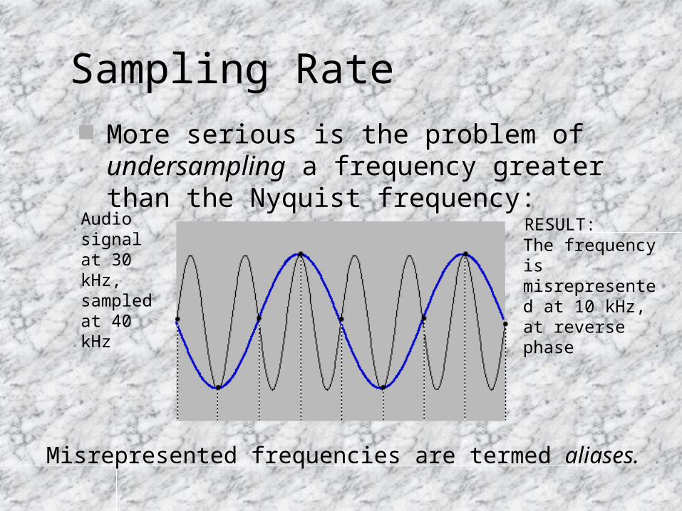
Sampling Rate More serious is the problem of undersampling a

frequency greater than the Nyquist frequency:

Audio signal at 30 kHz,sampled at 40 kHz

RESULT:

Sampling Rate More serious is the problem of undersampling a

frequency greater than the Nyquist frequency:

Audio signal at 30 kHz,sampled at 40 kHz

RESULT:The frequency is misrepresented at 10 kHz, at reverse phase

Misrepresented frequencies are termed aliases.

Sampling Rate

In general, if a frequency, F, sampled at a sampling rate of SR, exceeds the Nyquist frequency, that frequency will alias to a frequency of:- (SR - F)

The minus sign indicates that the frequency is in opposite phase

Sampling Rate It is useful to illustrate sampled frequencies on a polar

diagram, with 0 Hz at 3:00 and the Nyquist frequency at 9:00:

0 HzNyquist

f

-f

The upper half of the circle represents frequencies from 0 Hz to the Nyquist frequency

The lower half of the circle represents negative frequencies from 0 Hz to the Nyquist frequency (there is no distinction in a digital audio system between ±NF)

Any audio frequency above the Nyquist frequency will alias to a frequency shown on the bottom half of the circle, a negative frequency between 0 Hz and the Nyquist frequency.

Frequencies above the Nyquist frequency do not exist in a digital audio system

Sampling Rate

In the recording process, filters are used to remove all frequencies above the Nyquist frequency before the audio signal is sampled.

This step is critical since aliases cannot be removed later.

Provided these frequencies are not in the sampled signal, the signal may be sampled and later reconverted to audio with no loss of information.

Sampling Rate

The sampling rate for audio CDs is 44.1 kHz.

Quantization

In the discussion of sampling rate, we only considered how often the amplitude of the wave was measured.

We did not discuss how accurate these measurements were.

The effectiveness of any measurement depends on the precision of our ruler. (Measuring the thickness of a book with a ruler only marking feet will probably not give a very accurate measurement.)

Just as there are limits to how often we can sample, there are limits to the resolution of our ruler.

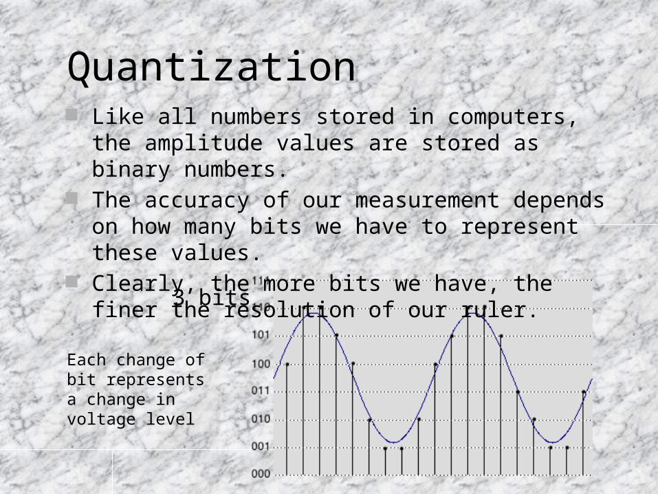
Quantization Like all numbers stored in computers, the amplitude values

are stored as binary numbers. The accuracy of our measurement depends on how many

bits we have to represent these values. Clearly, the more bits we have, the finer the resolution of

our ruler.

2 bits

Each change of bit represents a change in voltage level

Quantization Like all numbers stored in computers, the amplitude values

are stored as binary numbers. The accuracy of our measurement depends on how many

bits we have to represent these values. Clearly, the more bits we have, the finer the resolution of

our ruler.

3 bits

Each change of bit represents a change in voltage level

Quantization Like all numbers stored in computers, the amplitude values

are stored as binary numbers. The accuracy of our measurement depends on how many

bits we have to represent these values. Clearly, the more bits we have, the finer the resolution of

our ruler.

4 bits

Each change of bit represents a change in voltage level

Quantization

CD audio uses 16-bit quantization.

Quantization

While aliasing is eliminated if our signal contains no frequencies above the Nyquist frequency, quantization error can never be completely eliminated.

Every sample is within a margin of error that is half the quantization level (the voltage change represented by the least significant bit).

Quantization

For a sine wave signal represented with n bits, the signal to error ratio is:

S/E (dB) = 6.02n + 1.76

The problem is that low-level signals do not use all available bits, and therefore the error level is greater.

Quantization While quantization error may be masked at high

audio levels, it can become audible at low levels:

Worst case: a sine wave fluctuating within one quantization increment is stored as a square wave

Thus, unlike the constant hissing noise of analog recordings, quantization error is correlated with the signal, and is thus a type of distortion, rather than noise.

Quantization

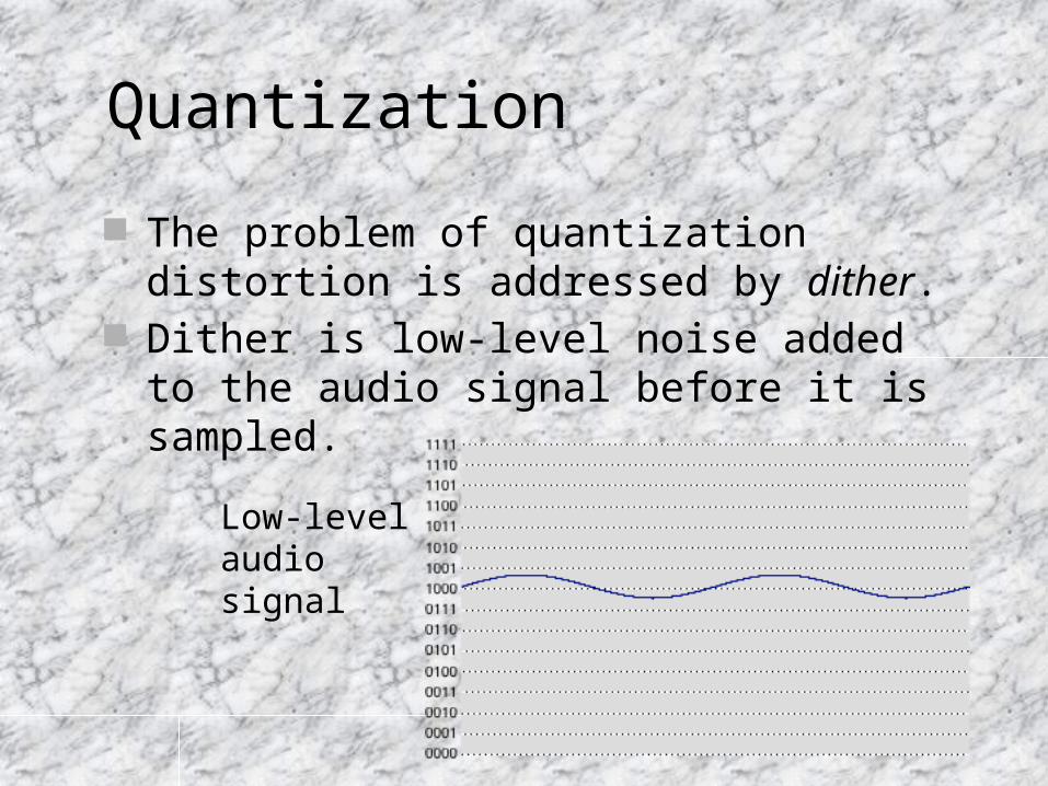
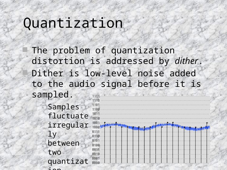
The problem of quantization distortion is addressed by dither.

Dither is low-level noise added to the audio signal before it is sampled.

Low-level audio signal

Quantization

The problem of quantization distortion is addressed by dither.

Dither is low-level noise added to the audio signal before it is sampled.

Samples fluctuate irregularly between two quantization levels

Quantization

Dither adds random errors to the signal, therefore the quantization results in added noise, rather than distortion.

The noise is a constant factor, not correlated with the signal like quantization distortion.

The result is a noisy signal, rather than a signal broken up by distortion.

Quantization

The auditory system averages the signal at all times. We do not hear individual samples.

With dither, this averaging allows the musical signal to co-exist with the noise, rather than be temporarily eliminated due to distortion.

Quantization

Dither allows resolution below the least significant quantization bit.

Without dither, digital recordings would be far less satisfactory than analog recordings.

With dither, there is significantly less noise in digital recordings than in analog recordings.

Quantization and Sampling Rate

The sampling rate determines the signal’s frequency content.

The number of quantization bits determines the amount of quantization error.

Size of Audio Files

44,100samples

per secondbytes per sample

(16 bits)

channels(for stereo

audio)

secondsper minute

x 2 x 2 x 60 ≈ 10 MB/minute