Computable Implementation of“Fundamental Theorem of Algebra”

Jon A. Sjogren1, Xinkai Li2, Mu Zhao2 and Chao Lu2

1Mail Stop 715, 2308 Mt. Vernon Ave.Alexandria VA 22301, USA

jsjogren8424@yahoo.com2Department of Computer & Information Sciences

Towson University, 8000 York RdTowson, MD 21252, USA

clu@towson.edu

June 5, 2013

Abstract

The Fundamental Theorem of Algebra (FTA) has beenstudied for more than 300 years: more or less satisfactoryproofs of FTA emerged in the 18th and 19th centuries.Proofs denoted as ‘algebraic’ or ‘elementary’ derived fromthe axioms defining a Real-Closed Field (RCF). A proof isgiven that brings up-to-date work of Gauss (1816) and P.Gordan (1879). It does not refer explicitly to the complexnumbers but instead works with auxiliary polynomials intwo variables. We report that computer software has beendeveloped to effect symbolic calculation in the context ofexact arithmetic. Some examples show how these routinesapply to the algebra of symmetric multinomial forms usedin Laplace’s proof (1795) of FTA, as well as to the theoryof Sylvester forms and the Bezoutian formulation of the re-sultant.

AMS Subject Classification: 08-02Keywords: Fundamental Theorem Algebra (FTA), Real

1

Closed Field (RCF), Symmetric Polynomial, Symbolic Cal-culation, Error-free Computing

1 Introduction

The historically important result known as the Fundamental The-orem of Algebra (FTA), which can also be named the Main Theo-rem on Complex Polynomials, has been studied for more than 300years. This proposition states that given a degree n>0 and com-plex numbers a0, ..., an−1 ∈ C, if we form the polynomial P (z) =zn + an−1z

n−1 + · · · + a0, there exists a complex value z0 whichserves as a zero for the polynomial considered as a function, namelyP (z0) = 0.

Until about 1840 it was usual to consider only polynomial func-tions of the form

f(X) = Xn + an−1Xn−1 + · · ·+ a0,

where all the aj are real, j = 0, . . . , n− 1.In fact the title of Gausss 1815 monograph was “. . . every in-

tegral rational algebraic function of one variable can be resolvedinto real factors of the first or second degree.” It gradually becameunderstood [27] that effecting this factorization (or solving for acomplex root) for f(X) would immediately solve the apparentlymore general case of (complex coefficients) P (z) referred above.

The more or less satisfactory proofs of FTA that emerged overthe 18th and 19th centuries provide a narrative on the state of math-ematical technique, and philosophy of rigor. The developing proofswere critical to the history of algebra and complex analysis espe-cially, but also involve logic/model theory, topology and algebraicgeometry. An entire book [13] is devoted to an exposition andcomparison of the various known classes of proof.

In this article we concentrate on a collection of proofs commonlydenoted as algebraic, with a view toward visualizing their stepscomputationally. The idea is to minimize the need for concepts ex-traneous to Algebra. It is known that the Theorem when applied tothe “standard real numbers” R requires attention to the transcen-dental properties of R. These properties, sufficient for FTA, areencapsulated in the axioms for a Real-Closed Field (RCF). Otherreal-closed fields include the hyper-reals R∗, the “constructive real

2

numbers” and the real algebraic numbers RA.An algebraic proof of FTA will apply to R, but equally well to

any RCF. In fact a few axioms characterize a real-closed field andthe proofs of interest employ these axioms and the rules of first-order predicate calculus. It is discussed in classic papers, owing to[34] and back to [3], that such derivations/theorems embody every-thing one could say about the real numbers in first-order sentences.Thus any two real-closed fields are elementarily equivalent .

We sum up the axioms of RCF somewhat informally. Sucha field F has an ordering compatible with the algebraic field op-erations, and the non-negative elements are precisely the perfectsquares. Besides this (we have so far a “formally real field”), an-other axiom is needed that takes various forms. For our purposes,this “Final Axiom” states that any odd-degree polynomial f(X)over the field has a root y ∈ F with f(y) = 0 (functional evalua-tion). If the axiom holds always for polynomials over F, this fieldis an RCF.

The formulation of FTA that we take is that for an RCF F,any polynomial f(X) factors into a number of polynomials of de-gree 1 (linear) and a number of irreducible polynomials of degree 2(quadratic). Calling factors of the first kind 1-factors and of thesecond kind 2-factors, we are concluding that any polynomial ofdegree >0 has a complete factorization (and unique up to scalarmultiples of the factors), that is, a complete 1, 2-factorization. Infact since f(X) is taken as monic, with leading coefficient equal to1, all the 1-and 2-factors can be taken as monic as well (compare“Gauss’s Lemma” [20]).

To get Gauss’s formulation from 1815, referred to as [16], it isonly necessary to show that the standard R satisfies the last axiomof RCF. This is where the transcendent definition of R (Bolzano-Weierstrass property) is indispensable. We give sketches of twoapproaches to this verification, one better known than the other, inthe following Section.

A discussion is pursued in the two Eureka articles [22], whichshows why, knowing that FTA actually holds (for the standardreals), there must be such an ‘elementary’ or first-order proof. Thuswe have miraculously proven, by means of meta-mathematics, thatFTA in Gauss’s form is immediately valid for other RCF such as thehyper-reals or “constructive real numbers”. The Eureka authors

3

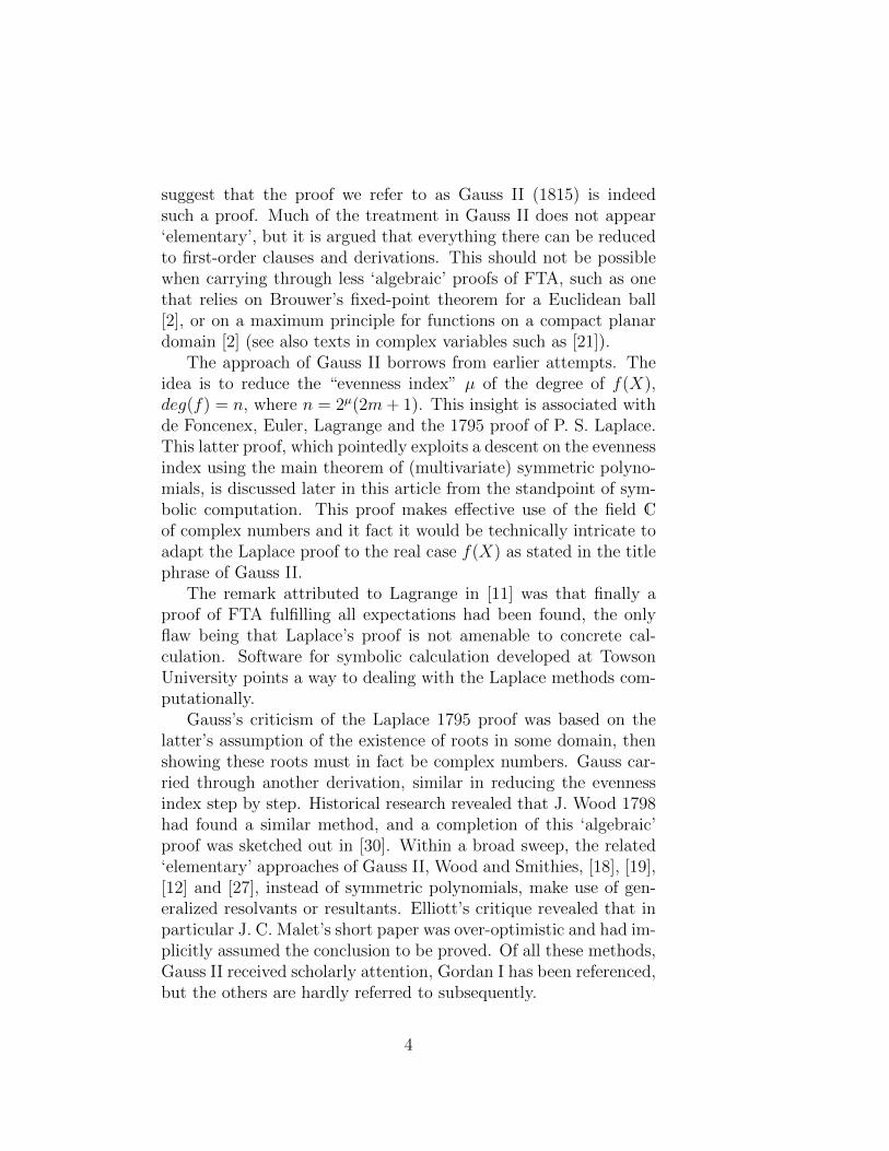
suggest that the proof we refer to as Gauss II (1815) is indeedsuch a proof. Much of the treatment in Gauss II does not appear‘elementary’, but it is argued that everything there can be reducedto first-order clauses and derivations. This should not be possiblewhen carrying through less ‘algebraic’ proofs of FTA, such as onethat relies on Brouwer’s fixed-point theorem for a Euclidean ball[2], or on a maximum principle for functions on a compact planardomain [2] (see also texts in complex variables such as [21]).

The approach of Gauss II borrows from earlier attempts. Theidea is to reduce the “evenness index” µ of the degree of f(X),deg(f) = n, where n = 2µ(2m+ 1). This insight is associated withde Foncenex, Euler, Lagrange and the 1795 proof of P. S. Laplace.This latter proof, which pointedly exploits a descent on the evennessindex using the main theorem of (multivariate) symmetric polyno-mials, is discussed later in this article from the standpoint of sym-bolic computation. This proof makes effective use of the field Cof complex numbers and it fact it would be technically intricate toadapt the Laplace proof to the real case f(X) as stated in the titlephrase of Gauss II.

The remark attributed to Lagrange in [11] was that finally aproof of FTA fulfilling all expectations had been found, the onlyflaw being that Laplace’s proof is not amenable to concrete cal-culation. Software for symbolic calculation developed at TowsonUniversity points a way to dealing with the Laplace methods com-putationally.

Gauss’s criticism of the Laplace 1795 proof was based on thelatter’s assumption of the existence of roots in some domain, thenshowing these roots must in fact be complex numbers. Gauss car-ried through another derivation, similar in reducing the evennessindex step by step. Historical research revealed that J. Wood 1798had found a similar method, and a completion of this ‘algebraic’proof was sketched out in [30]. Within a broad sweep, the related‘elementary’ approaches of Gauss II, Wood and Smithies, [18], [19],[12] and [27], instead of symmetric polynomials, make use of gen-eralized resolvants or resultants. Elliott’s critique revealed that inparticular J. C. Malet’s short paper was over-optimistic and had im-plicitly assumed the conclusion to be proved. Of all these methods,Gauss II received scholarly attention, Gordan I has been referenced,but the others are hardly referred to subsequently.

4

In fact the second treatment by Gordan II, 1885, in his com-pendium on Invariant Theory, is close to the Wood-Smithies proof,certainly giving more detail on the application of the Resultant.Nonetheless there is something to be gained by taking advantage ofprogress made in the 130 years since Gordan’s tome appeared. Forinstance, it can be useful to work with polynomials and resultantsdefined over a commutative ring more general than a field, whichwas not worked out in Gordan’s book. The approach of Gauss IIand others starts with the definition of the given polynomial overthe real field, and we proceed with the construction of 1- and 2-factors without requiring the preconception of a general algebraicclosure C = R[

√−1]. Thus we are taking a point of view similar

to when imaginary numbers were used, but on an ad hoc basis (saybefore Argand, Cauchy et al).

2 Transcendental Component of FTA

To do an induction on “evenness index” requires a base case whichis the “Final Axiom” concerned with odd-degree polynomials. Inthe case of the standard reals R, this principle is proved with thebasic Bolzano-Weierstrass defining property of R, which amountsto the fact that an open interval (a, b) is topologically connected,with topology induced from the usual metric on Q ⊂ R.

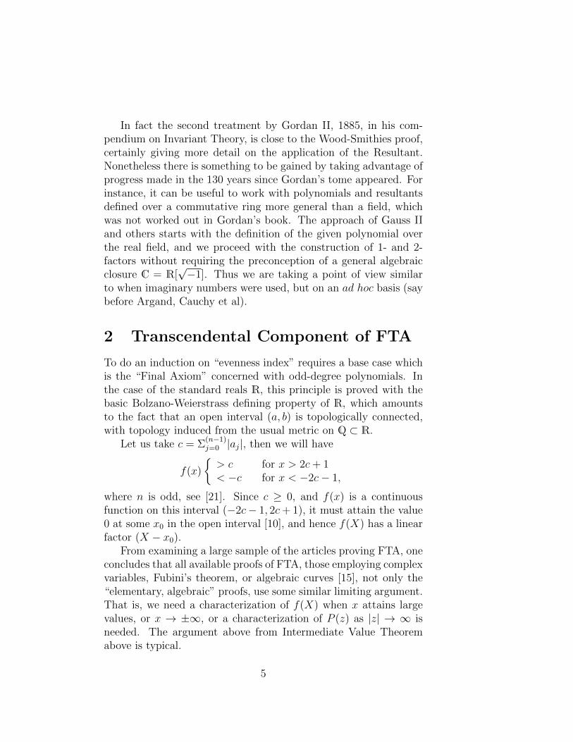
Let us take c = Σ(n−1)j=0 |aj|, then we will have

f(x)

{> c for x > 2c+ 1< −c for x < −2c− 1,

where n is odd, see [21]. Since c ≥ 0, and f(x) is a continuousfunction on this interval (−2c− 1, 2c+ 1), it must attain the value0 at some x0 in the open interval [10], and hence f(X) has a linearfactor (X − x0).

From examining a large sample of the articles proving FTA, oneconcludes that all available proofs of FTA, those employing complexvariables, Fubini’s theorem, or algebraic curves [15], not only the“elementary, algebraic” proofs, use some similar limiting argument.That is, we need a characterization of f(X) when x attains largevalues, or x → ±∞, or a characterization of P (z) as |z| → ∞ isneeded. The argument above from Intermediate Value Theoremabove is typical.

5

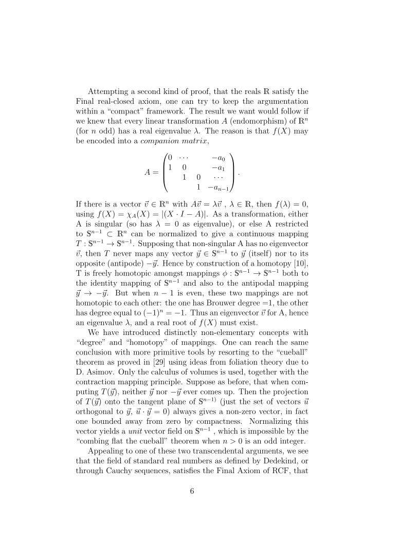
Attempting a second kind of proof, that the reals R satisfy theFinal real-closed axiom, one can try to keep the argumentationwithin a “compact” framework. The result we want would follow ifwe knew that every linear transformation A (endomorphism) of Rn

(for n odd) has a real eigenvalue λ. The reason is that f(X) maybe encoded into a companion matrix,

A =

0 · · · −a01 0 −a1

1 0 · · ·1 −an−1

.

If there is a vector ~v ∈ Rn with A~v = λ~v , λ ∈ R, then f(λ) = 0,using f(X) = χA(X) = |(X · I − A)|. As a transformation, eitherA is singular (so has λ = 0 as eigenvalue), or else A restrictedto Sn−1 ⊂ Rn can be normalized to give a continuous mappingT : Sn−1 → Sn−1. Supposing that non-singular A has no eigenvector~v, then T never maps any vector ~y ∈ Sn−1 to ~y (itself) nor to itsopposite (antipode) −~y. Hence by construction of a homotopy [10],T is freely homotopic amongst mappings φ : Sn−1 → Sn−1 both tothe identity mapping of Sn−1 and also to the antipodal mapping~y → −~y. But when n − 1 is even, these two mappings are nothomotopic to each other: the one has Brouwer degree =1, the otherhas degree equal to (−1)n = −1. Thus an eigenvector ~v for A, hencean eigenvalue λ, and a real root of f(X) must exist.

We have introduced distinctly non-elementary concepts with“degree” and “homotopy” of mappings. One can reach the sameconclusion with more primitive tools by resorting to the “cueball”theorem as proved in [29] using ideas from foliation theory due toD. Asimov. Only the calculus of volumes is used, together with thecontraction mapping principle. Suppose as before, that when com-puting T (~y), neither ~y nor −~y ever comes up. Then the projectionof T (~y) onto the tangent plane of Sn−1) (just the set of vectors ~uorthogonal to ~y, ~u · ~y = 0) always gives a non-zero vector, in factone bounded away from zero by compactness. Normalizing thisvector yields a unit vector field on Sn−1 , which is impossible by the“combing flat the cueball” theorem when n > 0 is an odd integer.

Appealing to one of these two transcendental arguments, we seethat the field of standard real numbers as defined by Dedekind, orthrough Cauchy sequences, satisfies the Final Axiom of RCF, that

6

odd-degree polynomials possess a root (zero).

3 Basic Determinantal Forms

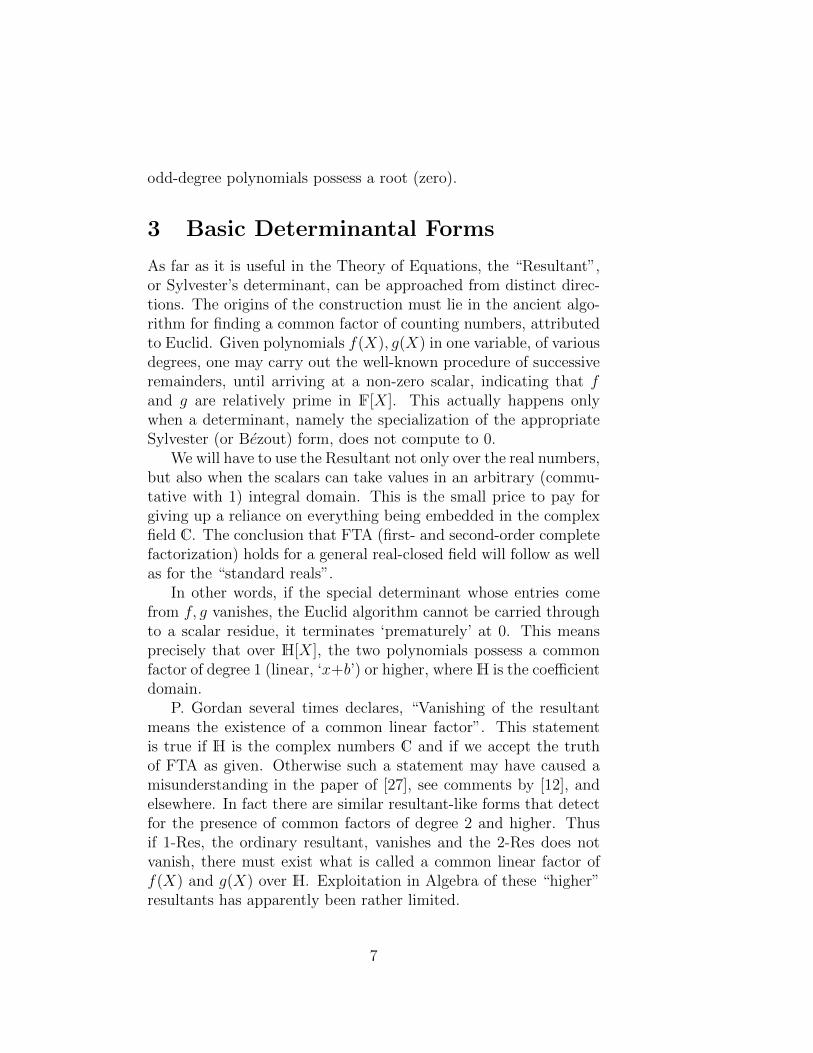
As far as it is useful in the Theory of Equations, the “Resultant”,or Sylvester’s determinant, can be approached from distinct direc-tions. The origins of the construction must lie in the ancient algo-rithm for finding a common factor of counting numbers, attributedto Euclid. Given polynomials f(X), g(X) in one variable, of variousdegrees, one may carry out the well-known procedure of successiveremainders, until arriving at a non-zero scalar, indicating that fand g are relatively prime in F[X]. This actually happens onlywhen a determinant, namely the specialization of the appropriateSylvester (or Bezout) form, does not compute to 0.

We will have to use the Resultant not only over the real numbers,but also when the scalars can take values in an arbitrary (commu-tative with 1) integral domain. This is the small price to pay forgiving up a reliance on everything being embedded in the complexfield C. The conclusion that FTA (first- and second-order completefactorization) holds for a general real-closed field will follow as wellas for the “standard reals”.

In other words, if the special determinant whose entries comefrom f, g vanishes, the Euclid algorithm cannot be carried throughto a scalar residue, it terminates ‘prematurely’ at 0. This meansprecisely that over H[X], the two polynomials possess a commonfactor of degree 1 (linear, ‘x+b’) or higher, whereH is the coefficientdomain.

P. Gordan several times declares, “Vanishing of the resultantmeans the existence of a common linear factor”. This statementis true if H is the complex numbers C and if we accept the truthof FTA as given. Otherwise such a statement may have caused amisunderstanding in the paper of [27], see comments by [12], andelsewhere. In fact there are similar resultant-like forms that detectfor the presence of common factors of degree 2 and higher. Thusif 1-Res, the ordinary resultant, vanishes and the 2-Res does notvanish, there must exist what is called a common linear factor off(X) and g(X) over H. Exploitation in Algebra of these “higher”resultants has apparently been rather limited.

7

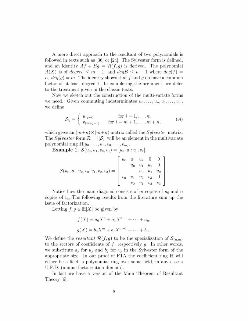
A more direct approach to the resultant of two polynomials isfollowed in texts such as [36] or [24]. The Sylvester form is defined,and an identity Af + Bg = R(f, g) is derived. The polynomialA(X) is of degree ≤ m − 1, and degB ≤ n − 1 where deg(f) =n, deg(g) = m. The identity shows that f and g do have a commonfactor of at least degree 1. In completing the argument, we deferto the treatment given in the classic texts.

Now we sketch out the construction of the multi-variate formswe need. Given commuting indeterminates u0, . . . , un, v0, . . . , vm,we define

Sij =

{u(j−i) for i = 1, . . . ,mv(m+j−1) for i = m+ 1, . . . ,m+ n,

(A)

which gives an (m+n)×(m+n) matrix called the Sylvester matrix.The Sylvester formR = |[S]| will be an element in the multivariatepolynomial ring H[u0, . . . , un, v0, . . . , vm].

Example 1. S(u0, u1, v0, v1) = [u0, u1; v0, v1],

S(u0, u1, u2, v0, v1, v2, v3) =

u0 u1 u2 0 0

u0 u1 u2 0u0 u1 u2

v0 v1 v2 v3 0v0 v1 v2 v3

.Notice how the main diagonal consists of m copies of u0 and n

copies of vm.The following results from the literature sum up theissue of factorization.

Letting f, g ∈ H[X] be given by

f(X) = a0Xn + a1X

n−1 + · · ·+ an,

g(X) = b0Xm + b1X

m−1 + · · ·+ bm.

We define the resultant R(f, g) to be the specialization of S{n,m}to the sectors of coefficients of f , respectively g. In other words,we substitute aj for uj and bj for vj in the Sylvester form of theappropriate size. In our proof of FTA the coefficient ring H willeither be a field, a polynomial ring over some field, in any case aU.F.D. (unique factorization domain).

In fact we have a version of the Main Theorem of ResultantTheory [6].

8

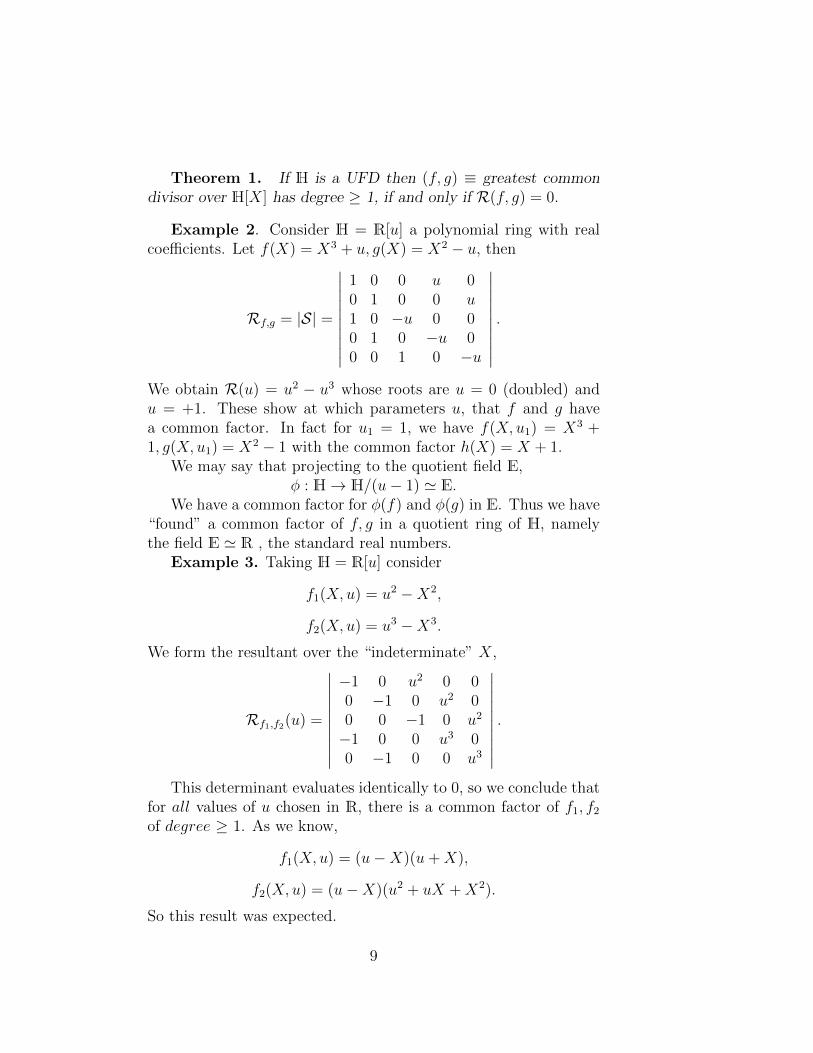
Theorem 1. If H is a UFD then (f, g) ≡ greatest commondivisor over H[X] has degree ≥ 1, if and only if R(f, g) = 0.

Example 2. Consider H = R[u] a polynomial ring with realcoefficients. Let f(X) = X3 + u, g(X) = X2 − u, then

Rf,g = |S| =

∣∣∣∣∣∣∣∣∣∣1 0 0 u 00 1 0 0 u1 0 −u 0 00 1 0 −u 00 0 1 0 −u

∣∣∣∣∣∣∣∣∣∣.

We obtain R(u) = u2 − u3 whose roots are u = 0 (doubled) andu = +1. These show at which parameters u, that f and g havea common factor. In fact for u1 = 1, we have f(X, u1) = X3 +1, g(X, u1) = X2 − 1 with the common factor h(X) = X + 1.

We may say that projecting to the quotient field E,φ : H→ H/(u− 1) ' E.

We have a common factor for φ(f) and φ(g) in E. Thus we have“found” a common factor of f, g in a quotient ring of H, namelythe field E ' R , the standard real numbers.

Example 3. Taking H = R[u] consider

f1(X, u) = u2 −X2,

f2(X, u) = u3 −X3.

We form the resultant over the “indeterminate” X,

Rf1,f2(u) =

∣∣∣∣∣∣∣∣∣∣−1 0 u2 0 00 −1 0 u2 00 0 −1 0 u2

−1 0 0 u3 00 −1 0 0 u3

∣∣∣∣∣∣∣∣∣∣.

This determinant evaluates identically to 0, so we conclude thatfor all values of u chosen in R, there is a common factor of f1, f2of degree ≥ 1. As we know,

f1(X, u) = (u−X)(u+X),

f2(X, u) = (u−X)(u2 + uX +X2).

So this result was expected.

9

4 Properties of the Resultant

The classic text of P. Gordan, Invariantentheorie (1885) demon-strates many properties within the context of the theory of deter-minants and other invariants. Only a few of these bear directly onour modified proof of FTA for real polynomials. With full appreci-ation for Gordan’s lively style, in some cases the treatment can bemade more understandable to the modern reader.

Recall that a multi-variant polynomial G(y0, . . . , yn) is calledhomogeneous of degree d if all the terms of G, typically

cα(0),α(1),...,α(n)yα(0)0 . . . yα(n)n

possess the same total degree =∑n

j=0 α(j) , recorded as long as

cα(0),α(1),...,α(n)yα(0)0 . . . yα(n)n 6= 0.

It is well-known [6] thatProposition 1. The polynomial G ∈ H[y0, . . . , yn] is homoge-

neous of degree d if and only if for any scalar λ ∈ H we calculate

G(λy0, . . . , λyn) = λdG(y0, . . . , yn).

Proposition 2. The Sylvester formR = |S(u0, . . . , un, v0, . . . , vm)|is homogeneous of degree m+ n.

Proof. The Sylvester matrix has size (m+ n)× (m+ n) . Sub-stituting λu0 for u0, λvj for vj etc, everywhere in this matrix hasthe effect of multiplying each row of S the scalar λ ∈ H. Now byfundamental property of the determinant “form”, we have

R(λu0, . . . , λvm) = λm+nR(u0, . . . , vm).

Hence by Proposition 1, R is homogeneous of degree m+ n.Definition 1. The weight of a multi-variable term

M = cα(0),α(1),...,α(n),β(0),β(1),...,β(m)uα(0)0 . . . uα(n)n v

β(0)0 ...vβ(m)

m

is defined as w(M) = Σni=0i · α(i) + Σm

j=0j · β(j). Thus for example,(u20u

31u

22v

50v

21v

23) = 7 + 8 = 15.

Definition 2. A form consisting of terms f = r1M1+ · · ·+rtMt

is said to be isobaric of weight p if rj 6= 0 implies w(Mj) = p forj = 1, . . . , t.

10

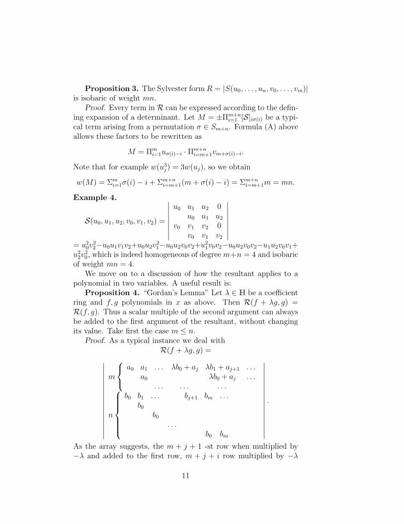
Proposition 3. The Sylvester formR = |S(u0, . . . , un, v0, . . . , vm)|is isobaric of weight mn.

Proof. Every term inR can be expressed according to the defin-ing expansion of a determinant. Let M = ±Πm+n

i=1 [S]iσ(i) be a typi-cal term arising from a permutation σ ∈ Sm+n. Formula (A) aboveallows these factors to be rewritten as

M = Πmi=1uσ(i)−i · Πm+n

i=m+1vm+σ(i)−i.

Note that for example w(u3j) = 3w(uj), so we obtain

w(M) = Σmi=1σ(i)− i+ Σm+n

i=m+1(m+ σ(i)− i) = Σm+ni=m+1m = mn.

Example 4.

S(u0, u1, u2, v0, v1, v2) =

∣∣∣∣∣∣∣∣u0 u1 u2 0

u0 u1 u2v0 v1 v2 0

v0 v1 v2

∣∣∣∣∣∣∣∣= u20v

22−u0u1v1v2+u0u2v21−u0u2v0v2+u21v0v2−u0u2v0v2−u1u2v0v1+

u22v20, which is indeed homogeneous of degree m+n = 4 and isobaric

of weight mn = 4.We move on to a discussion of how the resultant applies to a

polynomial in two variables. A useful result is:Proposition 4. “Gordan’s Lemma” Let λ ∈ H be a coefficient

ring and f, g polynomials in x as above. Then R(f + λg, g) =R(f, g). Thus a scalar multiple of the second argument can alwaysbe added to the first argument of the resultant, without changingits value. Take first the case m ≤ n.

Proof. As a typical instance we deal withR(f + λg, g) =∣∣∣∣∣∣∣∣∣∣∣∣∣∣∣∣

m

a0 a1 . . . λb0 + aj λb1 + aj+1 . . .

a0 λb0 + aj . . .. . . . . . . . .

n

b0 b1 . . . bj+1 bm . . .

b0b0

. . .b0 bm

∣∣∣∣∣∣∣∣∣∣∣∣∣∣∣∣.

As the array suggests, the m + j + 1 -st row when multiplied by−λ and added to the first row, m + j + i row multiplied by −λ

11

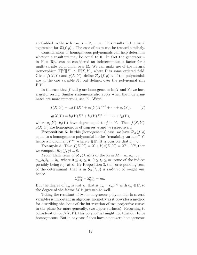
and added to the i-th row, i = 2, . . . , n. This results in the usualexpression for R(f, g) . The case of n<m can be treated similarly.

Consideration of homogeneous polynomials can help determinewhether a resultant may be equal to 0. In fact the generator uin H = R[u] can be considered an indeterminate, a factor for amulti-variate polynomial over R. We can make use of the naturalisomorphism F[Y ][X] ' F[X, Y ], where F is some ordered field.Given f(X, Y ) and g(X, Y ), define RX(f, g) as if the polynomialsare in the one variable X, but defined over the polynomial ringF[Y ].

In the case that f and g are homogeneous in X and Y , we havea useful result. Similar statements also apply when the indetermi-nates are more numerous, see [6]. Write

f(X, Y ) = a0(Y )Xn + a1(Y )Xn−1 + · · ·+ an(Y ), (I)

g(X, Y ) = b0(Y )Xn + b1(Y )Xn−1 + · · ·+ bn(Y ),

where aj(Y ), bj(Y ) have degree equal to j in Y . Then f(X, Y ),g(X, Y ) are homogeneous of degrees n and m respectively.

Proposition 5. In this (homogeneous) case, we have RX(f, g)equal to a homogeneous polynomial in the “remaining variable” Y ,hence a monomial cY mn where c ∈ F. It is possible that c = 0.

Example 5. Take f(X, Y ) = X + Y, g(X, Y ) = X3 + Y 3, thenwe compute RX(f, g) ≡ 0.

Proof. Each term of RX(f, g) is of the form M = as1as2 . . .asmbt1bt2 . . . btn where 0 ≤ sρ ≤ n, 0 ≤ tε ≤ m, some of the indicespossibly being repeated. By Proposition 3, the corresponding termof the determinant, that is in SX(f, g) is isobaric of weight mn,hence

Σmsρρ=1 + Σntε

ε=1 = mn.

But the degree of asl is just sl, that is asl = cslYsl with csl ∈ F, so

the degree of the factor M is just mn as well.Taking the resultant of two homogeneous polynomials in several

variables is important in algebraic geometry as it provides a methodfor describing the locus of the intersection of two projective curvesin the plane (or more generally, two hyper-surfaces). Returning toconsideration of f(X, Y ), this polynomial might not turn out to behomogeneous. But in any case f does have a non-zero homogeneous

12

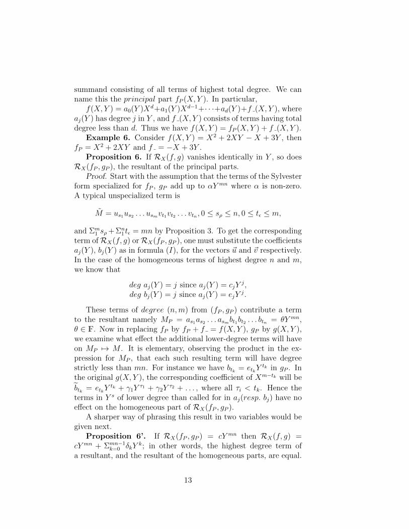
summand consisting of all terms of highest total degree. We canname this the principal part fP (X, Y ). In particular,

f(X, Y ) = a0(Y )Xd+a1(Y )Xd−1+· · ·+ad(Y )+f (X, Y ), whereaj(Y ) has degree j in Y , and f (X, Y ) consists of terms having totaldegree less than d. Thus we have f(X, Y ) = fP (X, Y ) + f (X, Y ).

Example 6. Consider f(X, Y ) = X2 + 2XY − X + 3Y , thenfP = X2 + 2XY and f = −X + 3Y .

Proposition 6. If RX(f, g) vanishes identically in Y , so doesRX(fP , gP ), the resultant of the principal parts.

Proof. Start with the assumption that the terms of the Sylvesterform specialized for fP , gP add up to αY mn where α is non-zero.A typical unspecialized term is

M = us1us2 . . . usmvt1vt2 . . . vtn , 0 ≤ sρ ≤ n, 0 ≤ tε ≤ m,

and Σm1 sρ + Σn

1 tε = mn by Proposition 3. To get the correspondingterm ofRX(f, g) orRX(fP , gP ), one must substitute the coefficientsaj(Y ), bj(Y ) as in formula (I), for the vectors ~u and ~v respectively.In the case of the homogeneous terms of highest degree n and m,we know that

deg aj(Y ) = j since aj(Y ) = cjYj,

deg bj(Y ) = j since aj(Y ) = ejYj.

These terms of degree (n,m) from (fP , gP ) contribute a termto the resultant namely MP = as1as2 . . . asmbt1bt2 . . . btn = θY mn,θ ∈ F. Now in replacing fP by fP + f = f(X, Y ), gP by g(X, Y ),we examine what effect the additional lower-degree terms will haveon MP 7→ M . It is elementary, observing the product in the ex-pression for MP , that each such resulting term will have degreestrictly less than mn. For instance we have btk = etkY

tk in gP . Inthe original g(X, Y ), the corresponding coefficient of Xm−tk will be

btk = etkYtk + γ1Y

τ1 + γ2Yτ2 + . . . , where all τi < tk. Hence the

terms in Y s of lower degree than called for in aj(resp. bj) have noeffect on the homogeneous part of RX(fP , gP ).

A sharper way of phrasing this result in two variables would begiven next.

Proposition 6’. If RX(fP , gP ) = cY mn then RX(f, g) =cY mn + Σmn−1

k=0 δkYk; in other words, the highest degree term of

a resultant, and the resultant of the homogeneous parts, are equal.

13

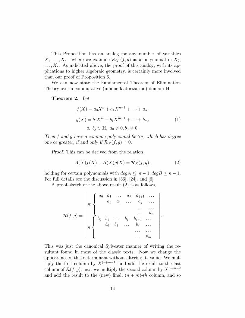
This Proposition has an analog for any number of variablesX1, . . . , Xr , where we examine RX1(f, g) as a polynomial in X2,. . . , Xr. As indicated above, the proof of this analog, with its ap-plications to higher algebraic geometry, is certainly more involvedthan our proof of Proposition 6.

We can now state the Fundamental Theorem of EliminationTheory over a commutative (unique factorization) domain H.

Theorem 2. Let

f(X) = a0Xn + a1X

n−1 + · · ·+ an,

g(X) = b0Xm + b1X

m−1 + · · ·+ bm, (1)

ai, bj ∈ H, a0 6= 0, b0 6= 0.

Then f and g have a common polynomial factor, which has degreeone or greater, if and only if RX(f, g) = 0.

Proof. This can be derived from the relation

A(X)f(X) +B(X)g(X) = RX(f, g), (2)

holding for certain polynomials with degA ≤ m− 1, degB ≤ n− 1.For full details see the discussion in [36], [24], and [6].

A proof-sketch of the above result (2) is as follows,

R(f, g) =

∣∣∣∣∣∣∣∣∣∣∣∣∣∣∣∣

m

a0 a1 . . . aj aj+1 . . .

a0 a1 . . . aj . . .. . . . . .. . . an

n

b0 b1 . . . bj bj+1 . . .

b0 b1 . . . bj . . .. . . . . .. . . bm

∣∣∣∣∣∣∣∣∣∣∣∣∣∣∣∣.

This was just the canonical Sylvester manner of writing the re-sultant found in most of the classic texts. Now we change theappearance of this determinant without altering its value. We mul-tiply the first column by X(n+m−1) and add the result to the lastcolumn of R(f, g); next we multiply the second column by Xn+m−2

and add the result to the (new) final, (n + m)-th column, and so

14

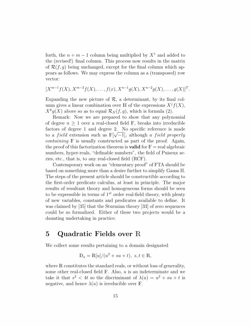
forth, the n+m− 1 column being multiplied by X1 and added tothe (revised!) final column. This process now results in the matrixof R(f, g) being unchanged, except for the final column which ap-pears as follows. We may express the column as a (transposed) rowvector:

[Xm−1f(X), Xm−2f(X), . . . , f(x), Xn−1g(X), Xn−2g(X), . . . , g(X)]T .

Expanding the new picture of R, a determinant, by its final col-umn gives a linear combination over H of the expressions Xjf(X),Xkg(X) above so as to equal RX(f, g), which is formula (2).

Remark: Now we are prepared to show that any polynomialof degree n ≥ 1 over a real-closed field F, breaks into irreduciblefactors of degree 1 and degree 2. No specific reference is madeto a field extension such as F[

√−1], although a field properly

containing F is usually constructed as part of the proof. Again,the proof of this factorization theorem is valid for F= real algebraicnumbers, hyper-reals, “definable numbers”, the field of Puiseux se-ries, etc., that is, to any real-closed field (RCF).

Contemporary work on an “elementary proof” of FTA should bebased on something more than a desire further to simplify Gauss II.The steps of the present article should be constructible according tothe first-order predicate calculus, at least in principle. The majorresults of resultant theory and homogeneous forms should be seento be expressible in terms of 1st order real-field theory, with plentyof new variables, constants and predicates available to define. Itwas claimed by [35] that the Sturmian theory [33] of zero sequencescould be so formalized. Either of these two projects would be adaunting undertaking in practice.

5 Quadratic Fields over R

We collect some results pertaining to a domain designated

Du = R[u]/(u2 + su+ t), s, t ∈ R,

whereR constitutes the standard reals, or without loss of generality,some other real-closed field F. Also, u is an indeterminate and wetake it that s2 < 4t so the discriminant of λ(u) = u2 + su + t isnegative, and hence λ(u) is irreducible over F.

15

The point of view taken is that the concept of “the complexnumbers C” has not been fully developed, at least for certain RCF,and thus we treat specific field extensions such as Du. Working ina polynomial ring modulo λ(u), we use only the simplest “field”constructions. Later one could prove that all these fields are iso-morphic to F(

√−1), but “field isomorphism” is not really relevant

to our approach toward FTA as this concept cannot be formulatedwithin the predicates of the theory of RCF.

Now it is easy to show that w ∈ Du can be written uniquely asγ + δu, with γ, δ ∈ F, by reducing a given polynomial in u moduloλ(u) a number of times. Furthermore there is a conjugation operator

χ : Du → Du

defined by χ(t) = t, t ∈ F, and χ(u) = u = −u − s, extended by

linearity. Note that χ(−u − s) = −(−u − s) − s = u, so χ2 = id,and we have an involution on Du.

χ-Property 1. Summing up, we have γ + δuχ−→ γ − δu− δs.

χ-Property 2. (w1 + w2) = χ(w1 + w2) = χ(w1) + χ(w2) =w1 + w2.

χ-Property 3. w1w2 = w1w2.Proof. We have w1w2 = γ1γ2 − δ1δ2t + (γ1δ2 + γ2δ1 − δ1δ2s)u,

hence χ(w1w2) = w1w2 = γ1γ2 − δ1δ2t + (γ1δ2 + γ2δ1 − δ1δ2s)u −(γ1δ2 − δ1δ2s)s.

On the other hand w1w2 = (γ1 − δ1u− δ1s) · (γ2 − δ2u− δ2s) =γ1γ2− γ1δ2s− γ2δ1s+ (−δ1γ2 + δ1δ2s− δ2γ1 + δ2δ1s)u+ δ1δ2(−su−t) + δ1δ2s

2.By comparing terms we observe that

χ(w1w2) = χ(w1)χ(w2).Definition 3. An element w ∈ Du is real if w = γ + δu with

δ = 0.χ-Property 4. The element w is real if and only if w = w.Proof. If w is real, δ = 0 so w = γ = w. conversely if w = w,

we have −δu− δs = δu which by uniqueness of the representationgives 2δ = 0. Since an ordered field has no torsion elements weconclude that δ = 0.

Next, we need to define conjugation applied to a polynomialf(X) ∈ Du[X] . Letting f(X) = c0X

n + c1Xn−1 + · · · + cn with

16

cj ∈ Du, j = 0, . . . , n , we define

χ(f) = f(X) = c0Xn + c1X

n−1 + · · ·+ cn,

and say that f ∈ Du[X] is real if the coefficients cj ∈ Du are real,that is cj = cj for all j. From the definitions we have:

χ-Property 5. The polynomial f(X) is real if and only iff = f . Next we treat the polynomial operations.

χ-Property 6. If g(X) = f1(X) + f2(X), k(X) = f1(X)f2(X),then g(X) = f 1(X) + f 2(X), k(X) = f 1(X)f 2(X).

Proof. The coefficient in the sum for Xj is the sum of the cor-responding coefficients and its conjugate equals the sum of theirconjugates, so we have the first result by χ-Property 2. For theproduct of two polynomials, its coefficients arise as entries in theconvolution of two sequences indexed byN , each with finitely many(bounded in number by the degree) non-zero entries. The convo-lution is computed as the sum of the products each of two factors,and conjugation is respected, according to χ-Property 2 and χ-Property 3, by both sum and product operations.

χ-Property 7. If f(X) divides real h(X) ∈ R[X] so does f(X).Proof. If h(X) = f(X)g(X) , conjugating both sides leads by

χ-Property 6 to the co-factor g(X) for f(X) in h(X) , where wemay use χ-Property 5 since h is real as a polynomial.

Note. There is no harm in writing φ(X) instead of φ(X) sinceX is unaffected by conjugation. However, if X is replaced by an-other expression in Du[X] it is best to apply the following.

χ-Property 8. If h(X) = f(g(X)) , then h(X) = f(g(X)).Proof. As a polynomial, f(X) is a linear combination of powers

of X , so h(X) will be a sum of terms typically cjg(X)j so theproblem reduces to “the conjugate of the power of a polynomial isequal to the same power taken of the conjugate” which is provedby induction on the power j, using χ-Property 6.

6 FTA by the Method of Laplace

In 1795, Laplace offered a convincing algebraic proof of FTA. Inhis proof, he used the theorem on symmetric functions which wasproved by Newton in 1673, it has also been known as fundamental

17

theorem of symmetric polynomials. Before introducing the funda-mental theorem of symmetric polynomials, several definitions needto be given.

Definition 4. A symmetric polynomial is a polynomial P (X1,X2, . . . , Xn) in n variables, such that if any two of the variables areinterchanged, one obtains the same polynomial.

Formally, P (X1, X2, . . . , Xn) is a symmetric polynomial, if forany permutation of the subscripts 1, 2, . . . , n, one has the same poly-nomial P (X1, X2, . . . , Xn). For example, in two variables X1, X2, asymmetric polynomial could appear as:

5X21X

22 +X2

1X2 +X22X1 + (X1 +X2)

2.

There are many ways to make specific symmetric polynomials inany number of variables such as

∏1≤i≤j≤n(Xi −Xj)

2.Definition 5. The elementary symmetric polynomials in n

variables X1 . . . Xn, written as ei(X1, . . . , Xn) for i = 0, 1, . . . , n,can be defined as e0(X1, X2, . . . , Xn) = 1, e1(X1, X2, . . . , Xn) =∑

1≤j≤nXj, e2(X1, X2, . . . , Xn) =∑

1≤j≤k≤nXjXk. And so forth,down to: en(X1, X2, . . . , Xn) = X1X2 . . . Xn

In general, for k ≥ 0 we define

ek(X1, . . . , Xn) =∑

1≤j1<j2<···<jk≤n

Xj1 , . . . , Xjk .

The elementary symmetric polynomials, power sum symmetric poly-nomials and complete homogeneous symmetric polynomials are threebasic blocks of symmetric polynomials used to generate the ring ofsymmetric polynomials in n variables.

The fundamental theorem of symmetric polynomials

Theorem 3. Any symmetric polynomial can be expressed asa polynomial in the elementary symmetric polynomials on thosevariables.

Proof. First, we review the definition of lexicographic order.The symmetric polynomial P (x1 . . . , xn)can be expressed as thesum of monomials of the form as cxi11 . . . x

inn , where ik is a nonneg-

ative integer. Then, the order on the monomials can be defined byspecifying that c1x

i11 . . . x

inn < c2x

j11 . . . x

jnn , when c2 6= 0 and there

18

is some 0 ≤ k ≤ n − 1 such that in−l = jn−l for l = 0, 1, . . . , k − 1but in−k < jn−k. For instance, 5x21x

32x

63 < 8x1x

42x

63. In other words,

starting in the nth position in both monomials, go back until thetwo exponents are not equal. The monomial with the larger expo-nent in that position has higher order. This is called a lexicographicorder on the monomials.

Suppose that cxi11 . . . xinn is the largest monomial in P . Then

we must have i1 ≤ i2 ≤ · · · ≤ in, otherwise this monomial is notthe largest one of P , because when P is symmetric, the polynomialP must also have the monomial cxj11 . . . x

jnn , where (j1, j2, . . . , jn)

is the sequence (i1, i2, . . . , in) sorted in increasing order. But thismonomial is larger than the monomial cxi11 . . . x

inn unless we have

i1 ≤ i2 ≤ · · · ≤ in. Thus, we can define a symmetric polynomial Rby R = ce

in−in−1

1 ein−1−in−2

2 . . . ei2−i1n−1 ei1n , where ek is the kth elemen-

tary symmetric polynomial in the n variables x1, . . . , xn. So thatR is a polynomial in the elementary symmetric polynomials. Alsowe can prove that the largest monomial of R equals to cxi11 . . . x

inn .

Because the largest monomial of R = cein−in−1

1 ein−1−in−2

2 . . . ei2−i1n−1 ei1n

equals to:

c · (largest monomial of e1)in−in−1 · (largest monomial of e2)in−1−in−2

. . . (largest monomial of en−1)i2−i1 ·(largest monomial of en)i1

= c(xn)in−in−1(xn−1xn)in−1−in−2 . . . (x2x3 . . . xn)i2−i1(x1x2x3 . . . xn)i1

= cxj11 . . . xjnn , since ek(X1, . . . , Xn) =

∑1≤i1≤i2≤···≤ik≤nXi1 . . . Xik

is the kth elementary symmetric polynomial.Therefore, we reduce P (x1, . . . , xn) by successively subtracting

a product of elementary symmetric polynomials to eliminate thelargest monomial without introducing any larger monomials. Thisway, in each step, the largest monomial is reduced until it becomeszero, and we get the sum of the subtracted-off polynomials, which isthe desired expression of P as a polynomial function of elementarypolynomials.

Example 7. Suppose we have a symmetric polynomial as thefollowing and we have written it in an increasing order:

P = x21x2 + x1x22 + x21x3 + 6x1x2x3 + x22x3 + x1x

23 + x2x

23.

The largest monomial is x2x23, so we subtract off e2−11 e1−02 e03,

which is e1e2, then we get:P − e1e2 = x21x2 + x1x

22 + x21x3 + 6x1x2x3 + x22x3 + x1x

23 + x2x

23−

(x1 + x2 + x3)(x1x2 + x1x3 + x2x3) = 3x1x2x3.

19

Now the largest monomial is 3x1x2x3, so we subtract off 3e1−11 e1−12 e13,which is 3e3, getting P − e1e2 − e3 = 3x1x2x3 − 3x1x2x3 = 0. Thisgives P = e1e2 + e3.

7 FTA by the Method of Resultants

On the face of it, the Fundamental Theorem of Algebra deals withjust one polynomial or ‘equation’,

f(X) = Xn + a1Xn−1 + + an = 0,

where aj ∈ F, the ground field, for j = 1, . . . , n. We may aswell write for our real-closed field of interest F the standard realnumbers R, since we know that the same first-order results, andessentially the proofs too, will hold for both. The coefficient a0 canbe omitted partly to ensure that f(X) is legitimately of degree n.In the Introduction several analytic methods were given to verifythat R is indeed ‘real-closed’, that is, in case n = 2m+ 1 is odd, asolution x0 ∈ R, f(x0) = 0 always exists.

The rest of the proof of FTA utilizes only algebraic means, mea-sures and methods. Some bookkeeping on the degree is necessary,if n = 2µ(2m+ 1), we call µ the “index of evenness” of n or simply“index”. The equation g(X) = 0 is said to be “easier to solve” thanf(X) = 0 when n′ = deg g(X) = 2µ

′(2m′ + 1) and

µ < µ, or µ′ = µ and m′ < m (in other words n′ < n). (L)

Thus “easier to solve” or “easier to factor” is really a relation be-tween the degrees of two polynomials, and has nothing to do withthe values of the coefficients. The relation on degrees can be writtenn′ <L n. The relation (L) then leads to a ready-made induction,reducing the problem of factorization of an n-polynomial to that ofone or more n’-polynomials. When µ = 0 there is always a linearfactor, as seen in the Introduction, which arises from a root x0 sothat f(X) = (X − x0)h(X), deg h(X) = n− 1.

The ordering defined by (L) above is a total (or linear) order onthe natural numbers N. This ordering also arises from the lexico-graphical ordering induced on the Cartesian product {ζ : N} with{2m+ 1, odd natural numbers} by the canonical ordering on N.

20

Let J be a property of polynomials in R[X]. We may introducethe concept, “the polynomial f satisfies the reduction criterion withrespect to J ”, as meaning that whenever g(X) is “easier to factor”than f , it satisfies J (g). We will set up the specific instance of thereduction criterion that we need further along. Next we summarizethe logic of the proof, which is based on [19], [30] and [37].

Definition 6. A 1-factor is a linear (degree one) factor of apolynomial g(X) ∈ R[X], a 2-factor is an irreducible degree-twofactor, so that g(X) = (X2 + sX + t)h(X), with the discriminants2 − 4t negative.

Definition 7. Given H a field or a UFD, a complete fac-torization into irreducibles is a sequence {hi(X1, . . . , Xr)}, i =1, . . . , k of irreducible multi-variable polynomials, whose productgives the polynomial g(X1, . . . , Xr), which is to be so decomposedor factorized.

Gauss’s Factorization Theorem. Under the conditions ofdefinition 7, any polynomial g(X1, . . . , Xr) has a complete factor-ization into irreducibles {hi} whose entries are unique except for arearrangement of the indices and scalar multiples [20].

Note that if a variable Y = Xi is singled out as distinguishedand g() has leading coefficient equal to 1 (“monic”) with respect toY , then all the irreducible factors can be chosen monic as well.

Definition 8. A complete 1,2-factorization of g(X) ∈ F(X) isjust a factorization into irreducibles such that each factor is eithera 1-factor or a 2-factor.

Lemma A. If deg f(X) = n = 2m + 1 is odd, then f(X) hasa linear factor arising from some “zero” x0 ∈ R, so that f(X) =(X − x0)h(X). Thus f(X) has a 1-factor.

Proof. This was established in Section 2, “Transcendental Com-ponent” for the standard real numbers and in general by the FinalAxiom of the theory of RCF.

Lemma B. Suppose that for all 0 < q ≤ n, deg(g) = q impliesthat g(X) has a 1-factor or a 2-factor. Then if deg f(X) = n, f hasa complete 1,2-factorization.

Proof. By hypothesis, f(X) has either a linear or irreduciblequadratic factor so

f(x) = (X − x0)g(X) or f(X) = (X2 + sX + t)h(X). (3)

If deg g(X) = 0 or deg h(X) = 0, we are done. Otherwise 1 ≤

21

deg g < n or 1 ≤ deg h < n as the case may be, an inductionhypothesis supplies a complete 1,2-factorization for g or h. Finally,the formulas are used to yield a complete 1, 2-factorization for f(X)as well.Our main result is:

Proposition 7. Any polynomial f(X) ∈ R[X] of degree n ≥ 1has a 1-factor (linear) or a 2-factor (quadratic irreducible).

Together with Lemma B, this Proposition yields, collecting scalarfactors:

Theorem 4. Fundamental Theorem of Algebra (for anyRCF F). Any monic polynomial f(X) ∈ F[X] has a complete 1,2-factorizaiton into monic factors that are unique up to a choice ofordering.

Before stating and proving the final lemmas that give Proposi-tion 7 and Theorem 4, we make explicit the Reduction Hypothesiswe wish to use. We repeat the wordage of Reduction Hypothesis afew times so that its significance is clearer.

Reduction Hypothesis for f(X). The polynomial f(X) inR[X] or F[X] satisfies the Reduction Hypothesis for “factorization”if every polynomial g(X) “easier to factor” than f(X), has a 1-factor or a 2-factor. Thus if deg g <L deg f , then g(X) satisfiesthe conclusion of Proposition 7.

Example 8. A polynomial f(X) of degree 12 that factors into afactor of degree 8 and one of degree 4 will gain a 1- or 2-factor fromthe factor of degree 4, since 4 <L 12 and assuming that f satisfiesthe Reduction Hypothesis. On the other hand, for a polynomialh(X) of degree 8 to satisfy RH would mean that every polynomialof degree 12, 20, 24, . . . , plus 2, 6, 10, . . . , would already be knownto possess a 1- or 2-factor.

Lemma C. Let f(X) ∈ R[X] be a reducible polynomial, withevery g(X) satisfying deg g(X) <L deg f(X) having a 1-factor or2-factor. [Simply, f(X) satisfies the Reduction Hypothesis withrespect to factorization.] Then f(X) has a 1-factor or a 2-factor.

Proof. Since f(X) is reducible, f(X) = g1(X)g2(X) wheredeg g1, deg g2 ≥ 1. We observe that both deg g1, deg g2 < deg f =n, and the index µ where deg g = 2µ(2m+ 1) is less than or equalto that of f for at least one of g1, g2. Putting these facts together,we find deg g1 <L deg f OR deg g2 <L deg f . By the Reduction

22

Hypothesis, the factor g1 or g2 satisfying this inequality has a 1-factor or a 2-factor, and this factor can be used as the required 1-or 2-factor for f(X). We give another version of Proposition 7.

Proposition 7’. Suppose that deg f(X) ≥ 3. Then f(X) isreducible in R[X]. Combined with Lemma C, this result wouldimmediately imply Proposition 7 and Theorem 4 (FTA).

Theorem 4’ (Alternate FTA) If f(X) is irreducible in R[X],then deg f ≤ 2.

Proof of Equivalence with Theorem 4. We have just seen howProposition 7’ or Theorem 4’ implies Theorem 4 (FTA). Conversely,suppose that FTA holds and f(X) is irreducible. But by FTA, f(X)has a 1-factor or 2-factor and hence must be equal to that factorup to a scalar multiple, thus has degree ≤ 2.

Remark about Proposition 7’: Of course if deg f = 3, wealready know by Lemma A that f has a 1-factor so is reducible.Also when deg f = 4, one can obtain a factorization of f(X) usingthe classical “Cardano resolvent” [32]. Hence the unknown degreevalues are even, n = deg f , starting with n = 6.

To finish the proof of Proposition 7, we need two technical re-sults.

Lemma D. Let f(X) ∈ R[X], with degf ≥ 3, be irreducibleand satisfy the Reduction Hypothesis for <L together with theproperty of 1,2-factorization. [Again, this means that any g(X)easier to factor than f(X) is known already to possess a 1- or 2-factor.] Then there exist s, t ∈ R with s2 < 4t such that over thequadratic field Du defined by s,t, we have that f(X) considered asan element of Du[X] factors non-trivially, and also f(X + u) andf(X − u) have a non-trivial common factor y(X, u) ∈ Du[X].

Lemma E. Suppose that f(X) ∈ R[X] with degf ≥ 2 is ir-reducible and satisfies the Reduction Hypothesis, furthermore thatover some quadratic field Du, there is a common factor y(X, u) off(X + u) and f(X − u). Then deg f(X) = 2.

These two results could be merged into one, but we separate twothreads of the unified proof. Combining them enables us to proveProposition 7’ and by the logic declaimed above, also Proposition7, Theorem 4 and Theorem 4’.

Proof of Proposition 7. The sequence of natural numbers 1 <L

3 <L 5 <L · · · <L 2 <L 6 . . . is a total order and well-founded (thereare no infinite decreasing sequences). Thus a complete induction

23

can be applied to all of NL. Alternatively, given at the outset apolynomial f(X) with deg f = n = 2µ(2m+1), one can modify theproof to deal only with the finite setN− = {r ∈ N : r < nµ}. In thismanner we could avoid dealing with infinite sequences of integers,limit elements (similar to limit ordinals under “set membership”relation), and deal only with finite collections. Now we start theinduction. We choose n as minimal under <L to be the degree ofsome polynomial f(X) ∈ R[X] that has no 1-factor or 2-factor. ByLemma C, f(X) is irreducible, and we may take n ≥ 3 , otherwisethe conclusion of Proposition 7 holds immediately. Hence all theantecedent conditions in Lemma D hold for f(X) . The consequentof Lemma D , together with the same antecedent conditions (RHand irreducibility) show also that the hypotheses of Lemma E aresatisfied. Therefore we arrive at the conclusion deg f = 2 as theonly remaining possibility, a blatant contradiction. Hence there isno such “least degree” n (with respect to <L), and no counter-example f(X) to Proposition 7.

There remains only to verify Lemmas D and E to complete theproof of FTA over a real-closed field. We highlight the principaltechnique used for Lemma D, and expand on the idea due to JamesWood of using a Resultant that arises from the original polynomial.

8 Factors over the Ring R[X ]

In keeping with the notation of [19] we write,

f(X) = Xn + a1Xn−1 + · · ·+ an(= 0),

with degf = n = 2µ(2m + 1). Now choose an indeterminate al-gebraically independent of X, called u. When n ≥ 2 we definepolynomials in R[X, u], F (X, u) = 1

2{f(X + u) + f(X − u)}, the

“even part”, and G(X, u) = 12u{f(X+u)−f(X−u)}, the “reduced

odd part”.Of interest is the resultant L(u) ≡ RX(F,G). But note that

f(X + u) = F (X, u) + uG(X, u).

By Gordan’s Lemma on resultants, the resultantRX(f(X+u), G(X, u))must be the same polynomial in u as L(u). Therefore L(u) deter-mines whether f(X + u) can be factored in common with G(X, u).We note some properties of this resultant, valid when ≥ 2

24

Property 1. Let FP (X, u), GP (X, u) be the respective “prin-cipal” homogeneous parts, which have total degrees n and (n− 1).Then RX(FP , GP ) is not identically 0 as a polynomial in u.

Proof. If this resultant were identically zero, it would mean that(X+u)n+(X−u)n and (X+u)n−(X−u)n would have a commonfactor in R[X, u], hence so would (X + u)n and (X − u)n , but thiswould violate the Gauss (unique) factorization theorem over thisring.

Property 2. We have deguL(u) = n(n−1) unless the principalhomogeneous part LP (u) = RX(FP , GP ) is zero.

Proof. The polynomials F (X, u) and G(X, u) have degree nand (n − 1) respectively, thus so do their principal homogeneousparts. By Proposition 5, their resultant has degree n(n− 1) unlessin fact RX(FP , GP ) = 0 identically. Thus according to Property 1,deguL(u) = n(n− 1) and we obtain the following.

Property 3. In fact L(u) = M(w) where u2 = w and (M) =12n(n− 1).Proof. By substituting values it can easily be seen that F

and G are even functions of u, hence even polynomials in u, overR[X]. Thus whenever u appears in the specialized Sylvester formSX(F,G), only entries depending on u2 = w appear. HenceRX(F,G)=determinant of the specialized Sylvester matrix, has only terms inpowers of w occurring, and we determine its degree from Properties1 and 2.

Property 4. M(w) is a polynomial “easier to factor” thanf(X).

Proof. It is only necessary to confirm that deg(M) <L deg(f) =n , which comes from Property 3.

Proof of Lemma D. We apply the construction above to f(X)which is assumed to satisfy the hypotheses of Lemma D. In view ofProperty 4, one concludes that M(w) has a 1- or 2-factor in R[w].

Now Case 1 occurs when the purported 1-factor is of the formk(w) = w−a. Take first the possibility that a ≥ 0, but then u2 = awith its solution

√a, which exists by the Axioms of a real-closed

field, would mean that f(X +√a) is reducible over R[X], hence so

is f(X), contradicting the hypothesis.Next we consider a < 0 when we set s = 0 and t = −a > 0, so

that by the Main Theorem of Resultants we deduce that f(X + u)has a factor β(X) whenever u2 = a, or expressed otherwise f(X)

25

is reducible in Du[X] where Du is defined by the parameters s =0, t = −a.

Case 2. If there is no 1-factor of M(w), there must be a 2-factorw2 + σw + τ, σ2 < 4τ .

Writing γ(u) = u4 + σu2 + τ , we arrive at a factor of γ, λ(u) =u2 + su+ t where s = {2

√τ −σ}1/2, t =

√τ which are defined in R

and satisfy s2 = 2√τ − σ < 4t = 4

√τ , since −σ < 2

√τ whatever

be the sign of σ.The complementary factor of γ(u) will be κ(u) = u2 − su + t.

Similar to what was done in Case 1, we may define the field Du

based on parameters (s, t), the polynomial λ(u) ∈ R[u], or theparameters (−s, t), the polynomial κ(u). When Case 1 leads to anirreducible u2 + t, or when in Case 2 we have irreducible λ(u) asabove, we observe that the resultant RX(F,G) vanishes in Du.

Hence by the Main Theorem of Resultants, F (X, u) and G(X, u)have a common factor in Du, and by Gordan’s Lemma, so do f(X+u) and G(X, u) have a common factor that we designate β(X, u).Noting that 1

u= u−1 = −1

t(s + u) in Du, we must have β(X, u)

also dividing f(X − u). Certainly then β(X − u, u) is a factor off(X) in Du[X] whose X-degree is greater than or equal to 1. ThusLemma D is established.

Proof of Lemma E. Since ε(X, u) divides f(X + u) over Du,the polynomial ε(X−u, u) will divide f(X). For the moment writeφ(X) = φu(X) = ε(X − u, u). Thus φ(X)ψ(X) = f(X) for someψ(X) ∈ Du[X]. By Lemma A, we have that n = deg f(X) is aneven natural number. First we show that the factor φ(X) in Du(X)must have X-degree = n/2. Otherwise if deg φ < n/2, we canchoose an irreducible factor φ1(X) dividing φ(X) in Du(X). Sincef(X) is real (has real coefficients), also φ1(X), the u-conjugate,divides f(X) by χ-Property 7. But φ1(X) is not real so by χ-Property 5 does not equal φ1(X), and both are irreducible withonly scalar factors in common. Also by χ-Property 5, φ1(X)φ1(X)is real, hence, f(X) = φ1(X)φ1(X)h(X) for a residual real factorh(X). Since deg φ1(X) = deg φ1(X), the irreducibility of f(X) inR[X] shows that the the only possibility is deg φ1 = deg φ = n/2 .We have at the same time proved that φu(X) must be irreduciblein Du (X). The complementary factor ψ(X) must equal φ(X) andbe irreducible as well. This fact comes up again later in the proof.

26

Recall the hypotheses of Lemma E. We have just shown that

f(X + u) = φ(X + u)ψ(X + u),

f(X − u) = φ(X − u)ψ(X − u)

with the factors displayed on the right-hand side being irreduciblein Du[X]. According to hypothesis, f(X + u) and f(X − u) have acommon factor. Up to a reflection symmetry, there are essentiallyonly two possibilities: φ(X+u) = φ(X−u) and φ(X+u) = ψ(X−u). Addressing the first choice, suppose that φ(X + u)− φ(X − u)equals the zero polynomial inX. Letting q = n/2−1, the only termsof this expression involvingXq come from the leading (monic) terms(X + u)q+1 and (X − u)q+1, so in the difference, these coefficientsare respectively (q + 1)u and −(q + 1)(−u), hence do not add tozero. Therefore φu(X + u) = φu(X − u) is impossible.

The second choice was that φ(X + u) = ψ(X − u) = φ(X − u)as polynomials over Du. Again if q + 1 = n/2, we write

φ(X + u) = (X + u)q+1 + c1(X + u)q + c2(X + u)q−1 + . . . ,

ψ(X − u) = (X − u)q+1 + c1(X − u)q + c2(X − u)q−1 + . . . ,

so the n/2 degree terms match up as before, but enumerating theterms in Xq give respectively (q + 1)u+ c1 from the first row, and−(q + 1)u + c1 from the second row. Writing c1 = a1 + b1u, weobtain c1 = (a1 − b1s)− b1u, and relying on unique representationof elements of Du, (q + 1 + b1)u = (−q − 1 − b1)u, a1 = a1 − b1s.Since Du is an integral domain, if b1 were equal to 0 we would have2(q + 1) = 0 as integers, thus q + 1 = 0 which is absurd. The onlyremaining possibility is s = 0, and in that case the characterizingpolynomial of Du must be of the form u2 + t = 0 with t > 0.

Since s = 0, we observe that χ(X − u) = X + u, hence in fact

φ(X + u) = ψ(X − u) = φ(X − u) = φ(X + u) = φ(X + u),

so by χ − Property 5 of u-conjugation, we deduce that φ(X +u) is actually real. In this last calculation, we also appealed toχ − Property 8 where the argument is X − u . Since its degreen/2 <L n, the polynomial φ(X +u) is “easier to factor” than f(X)and hence by the standard hypothesis (RH) built into Lemma E,we obtain that φ(X +u) has a 1-factor or a 2-factor in R[X]. That

27

means that in case deg φ > 2 , it follows that φ(X +u) is reduciblein R[X], hence φ(X) is reducible in Du which contradicts what wealready have established. If deg(φ) = 1, we have deg f(X) = 2 andthe conclusion of Lemma E holds. The only remaining case occurswhen deg φ(X) = 2. This means that deg f(X) = 4, so Cardano’sformulas can be applied to obtain a factorization of f(X). Anotherway is to reason that since the parameter s equals zero, φ(X) isautomatically reducible over Du[X]. More explicitly, a quadraticφ(X) = X2 + c1X + c2 can be factored by “completing the square”as long as every element a+ bu in Du has a square root. Recallingthat the parameters (s, t) = (0, t) for Du in our present situation,we have the explicit formula, similar to one we have seen earlier,for solving y2 = a+ bu, namely

±y =1√2{√a+√a2 + b2t+ sgn(b)u

√−a/t+

√(a/t)2 + b2/t},

where sgn(b) = b/|b| .This formula and the factorization of φ(X) can be verified by ex-

plicit arithmetic. But φ was determined to be irreducible in Du[X],so this case of deg φ = 2 is moot.

We completed an examination of the “second choice”, namelyφ(X + u) = ψ(X − u), which was refuted, leading inevitably todeg f(X) ≤ 2, the conclusion of Lemma E. We indicated earlierhow induction based on the <L ordering, and application of Lem-mas D and E, yields Propositions 7 and 7’, Theorem 4 and theFundamental Theorem of Algebra.

9 Computer Implementation

In this section, we report the computer implementation, which hasbeen developed to affect symbolic calculation in the context of ex-act arithmetic. Some examples show how these routines apply tothe algebra of symmetric multinomial forms used in Laplaces proof(1795) of FTA, as well as to the theory of Sylvester forms and theBezoutian formulation of the resultant.Laplace’s Method

Once the symmetric polynomials are represented by elementarypolynomials, we could see a more complex polynomial, which has

28

important form in Laplaces proof. Suppose ek is the kth elemen-tary symmetric polynomial in the n variables x1, . . . , xn. Then, ifwe have (x) =

∏{x− Ti(h, x1, . . . , xn)} , where Ti is polynomial of

h, x1, . . . , xn, and h is constant, we could express F in terms of ele-mentary polynomials through several steps. Here we give a simpleexample to explain the process.

Example 9. Consider ei(x1, x2, x3, x4) to be the elementarysymmetric polynomial of x1, x2, x3, x4, which is also a monic-univariatepolynomials. So that,

e1(x1, . . . , x4) = x1 + x2 + x3 + x4e2(x1, . . . , x4) = x1x2 + x1x3 + x1x4 + x2x3 + x2x4 + x3x4e3(x1, . . . , x4) = x1x2x3 + x1x2x4 + x1x3x4 + x2x3x4e4(x1, . . . , x4) = x1x2x3x4.

Write F (x) =∏{x − (x1 + x2 + x1x2)} · {x − (x1 + x3 +

x1x3)} . . . {x− (x3 + x4 + x3x4)} in terms of ei(x1, x2, x3, x4).Solution: We could write F (x) =

∏{x−T1}·{x−T2} . . . {x−T6}

at first, where T1 = x1 + x2 + x1x2 and so on. After expansionof F (x), the coefficient of F (x) should be elementary symmetricpolynomial ek(T1, T2, . . . , T6), k = 1, 2, . . . , 6. F (x) can be expressedas:

F (x) = x6 − e1(T1, T2, . . . , T6) · x5 + e2(T1, T2, . . . , T6) · x4 −e3(T1, T2, . . . , T6) ·x3 +e4(T1, T2, . . . , T6) ·x2−e5(T1, T2, . . . , T6) ·x+e2(T1, T2, . . . , T6).

Now, we rewrite ek(T1, T2, . . . , T6) in terms of ei(x1, x2, x3, x4).First, it is obvious that ek(T1, T2, . . . , T6) is also a function of x. Forexample, e1(T1, T2, . . . , T6) equals to: T1 + T2 + T3 + T4 + T5 + T6.And this equals to: 3(x1+x2+x3+x4)+x1x2+x1x3+x1x4+x2x3+x2x4+x3x4, which can also be rewritten in terms of ei(x1, x2, x3, x4)as 3e1(x1, x2, x3, x4) + e2(x1, x2, x3, x4).

Follow the same process, we could get all ek(T1, T2, . . . , T6) interms of ei(x1, x2, x3, x4) and we substitute them back into F (x).

Once we have the mathematical proof and structure, we canhand over the tedious work to a computer and let it generate thedetail formulas for us. Here we provide the core loop to implementthe process as follows:

Step 1: Input number of variables n and generate ei(x1, . . . , x6), i =1, . . . , n, which are the elementary polynomials of xi.

Step 2: F (x) =∏k

i=1{x− Ti(h, x1, x2, . . . , xn)} =∏k

i=1(−1)i−1 ·ek+1−i(T1, . . . , Tk) · xi−1, where Ti(.) can be any function of h and

29

xi. And k must be a number to ensure that the product of Ti(.) issymmetric function, where k depends on the form of Ti(.) and n.

Step 3: Express ek(T1, T2, . . . , Tk)in terms of ei(x1, . . . , xn);Write ek(T1, T2, . . . , Tk) in terms of x1, x2, . . . , xn as increasing

order so that the largest monomial equals to xi11 . . . xinn;

Follow the method introduced in the proof of FTA and translateek(T1, T2, . . . , Tk) to ei(x1, . . . , xn).

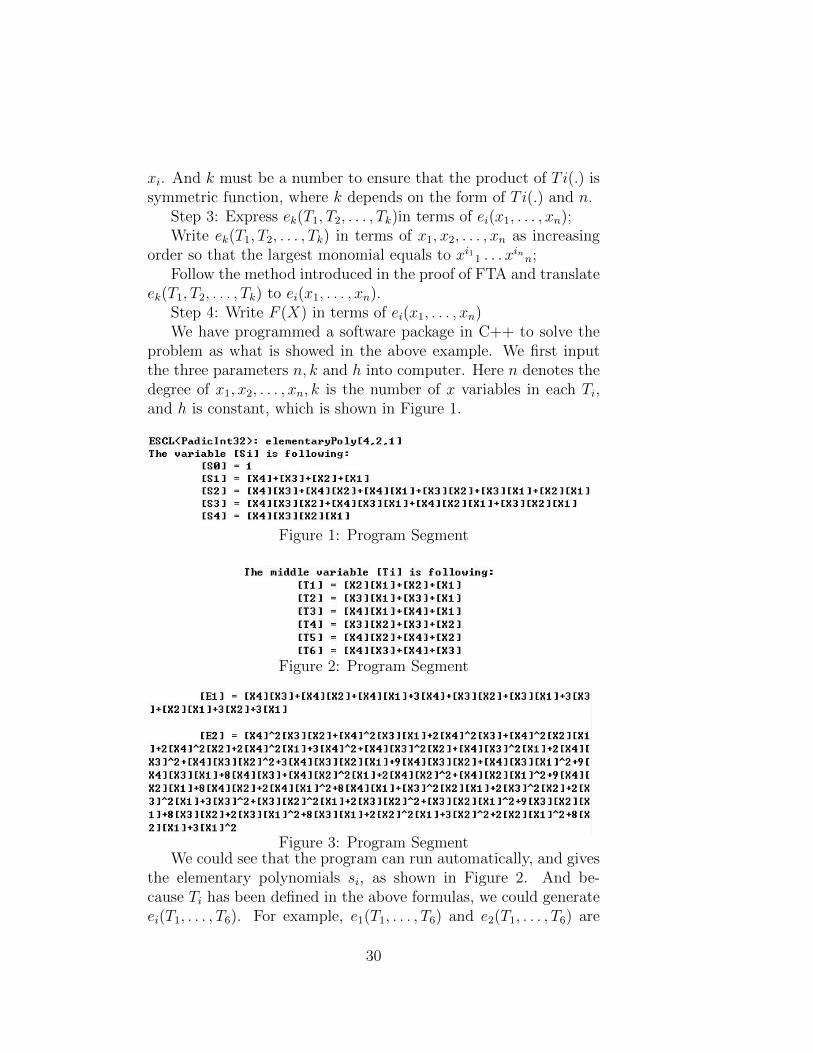
Step 4: Write F (X) in terms of ei(x1, . . . , xn)We have programmed a software package in C++ to solve the

problem as what is showed in the above example. We first inputthe three parameters n, k and h into computer. Here n denotes thedegree of x1, x2, . . . , xn, k is the number of x variables in each Ti,and h is constant, which is shown in Figure 1.

Figure 1: Program Segment

Figure 2: Program Segment

Figure 3: Program SegmentWe could see that the program can run automatically, and gives

the elementary polynomials si, as shown in Figure 2. And be-cause Ti has been defined in the above formulas, we could generateei(T1, . . . , T6). For example, e1(T1, . . . , T6) and e2(T1, . . . , T6) are

30

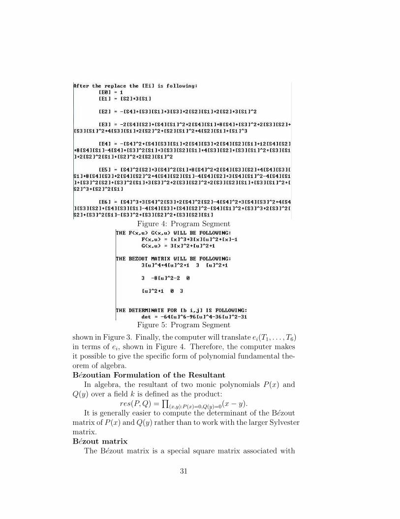
Figure 4: Program Segment

Figure 5: Program Segment

shown in Figure 3. Finally, the computer will translate ei(T1, . . . , T6)in terms of ei, shown in Figure 4. Therefore, the computer makesit possible to give the specific form of polynomial fundamental the-orem of algebra.Bezoutian Formulation of the Resultant

In algebra, the resultant of two monic polynomials P (x) andQ(y) over a field k is defined as the product:

res(P,Q) =∏

(x,y):P (x)=0,Q(y)=0(x− y).It is generally easier to compute the determinant of the Bezout

matrix of P (x) andQ(y) rather than to work with the larger Sylvestermatrix.Bezout matrix

The Bezout matrix is a special square matrix associated with

31

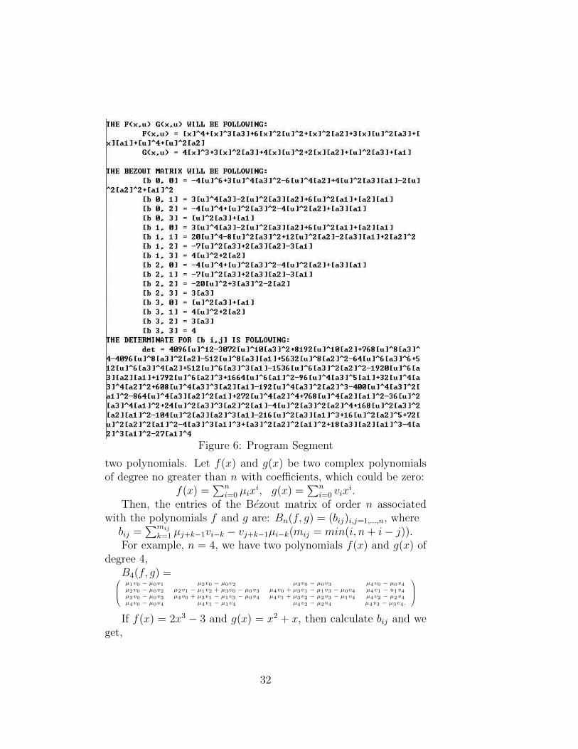
Figure 6: Program Segment

two polynomials. Let f(x) and g(x) be two complex polynomialsof degree no greater than n with coefficients, which could be zero:

f(x) =∑n

i=0 µixi, g(x) =

∑ni=0 vix

i.Then, the entries of the Bezout matrix of order n associated

with the polynomials f and g are: Bn(f, g) = (bij)i,j=1,...,n, wherebij =

∑mijk=1 µj+k−1vi−k − vj+k−1µi−k(mij = min(i, n+ i− j)).

For example, n = 4, we have two polynomials f(x) and g(x) ofdegree 4,

B4(f, g) =µ1v0 − µ0v1 µ2v0 − µ0v2 µ3v0 − µ0v3 µ4v0 − µ0v4µ2v0 − µ0v2 µ2v1 − µ1v2 + µ3v0 − µ0v3 µ4v0 + µ3v1 − µ1v3 − µ0v4 µ4v1 − u1v4µ3v0 − µ0v3 µ4v0 + µ3v1 − µ1v3 − µ0v4 µ4v1 + µ3v2 − µ2v3 − µ1v4 µ4v2 − µ2v4µ4v0 − µ0v4 µ4v1 − µ1v4 µ4v2 − µ2v4 µ4v3 − µ3v4.

If f(x) = 2x3 − 3 and g(x) = x2 + x, then calculate bij and we

get,

32

B3(f, g) =

3 3 03 0 20 2 2

.

Also, we can see that the Bezout matrix is symmetric.Computing process

We apply the resultant computation method in our modifiedWood-Gordan proof. Then the Q(v) can be obtained through thefollowing steps:

Step 1: f(x) has a degree n = 2qP , where P is odd and q ≥ 1.We assume q = 1, P = 3 and

f(x) = x6 − e1x5 + e2x4 − e3x3 + e4x

2 − e5x+ e6.Step 2: Construct the polynomials F (x, u) and G(x, u) accord-

ing to the following rules:{F (x, u) = 1

2[f(x+ u) + f(x− u)]

G(x, u) = u−1

2[f(x+ u)− f(x− u)]

F (x, u) = x6 − e1x5 + (e2 + 15u2)x4 + (−e3 − 10e1u2)x3 + (e4 +

6e2u2 + 15u4)x2 + (−e5 − 3e3u

2 − 5e1u4)x+ (e6 + e4u

2 + e2u4 + u6)

G(x, u) = 6x6 − 5e1x4 + (4e2 + 20u2)x3 + (−3e3 − 10e1u

2)x2 +(2e4 + 4e2u

2 + 6u4)x+ (−e5 − e3u2 − e1u4)Step 3: Construct Bezout matrix of F (x, u) and G(x, u) in re-

gard of x, B6(F,E) = (bij)i,j=1,...,6, wherebij =

∑mijk=1 µj+k−1vi−k − vj+k−1µi−k (mij = min(i, 6 + i− j)).

Since the entries of the matrix bij are quite complicated, we willnot provide full details here. However, they are all polynomials asbij(u, e1, . . . , e6).

Step 4: Since the resultant R(u) of F and G is exactly thedeterminant of Bezout matrix of F and G. We will compute thedeterminant of the matrix B6(F,G). Then we can get R(u), whichis of degree 30, and consists only of terms in u2, u4, . . . , u30.

Step 5: Let v = u2, we get the Q(v), which is of degree 15.Following this process, we get the exact form of Q(v) when q = 1

and P = 3, and we can get other Q(v) when P is odd and q ≥ 1analogously.Implementation on a computer

Example 9. Examining for practice the case of polynomialf(x) = x3 + x − 1, which does not need a reduction in index, theimplementation is shown in Figure 5.

Example 10. Given f(x) = x4 + a3x3 + a2x

2 + a1x+ a0, thenthe implementation is shown in Figure 6.

33

10 Software Design Considerations

10.1 The general structure of C++ package

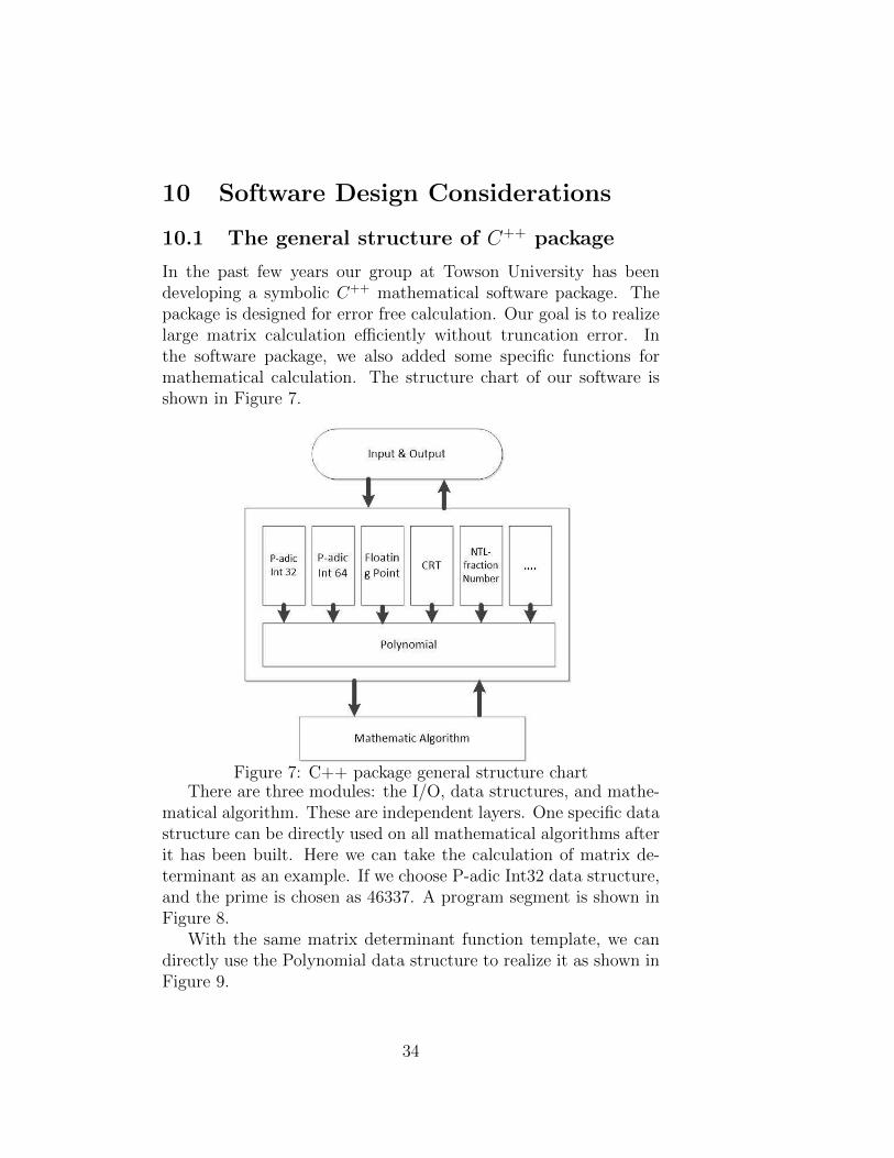
In the past few years our group at Towson University has beendeveloping a symbolic C++ mathematical software package. Thepackage is designed for error free calculation. Our goal is to realizelarge matrix calculation efficiently without truncation error. Inthe software package, we also added some specific functions formathematical calculation. The structure chart of our software isshown in Figure 7.

Figure 7: C++ package general structure chartThere are three modules: the I/O, data structures, and mathe-

matical algorithm. These are independent layers. One specific datastructure can be directly used on all mathematical algorithms afterit has been built. Here we can take the calculation of matrix de-terminant as an example. If we choose P-adic Int32 data structure,and the prime is chosen as 46337. A program segment is shown inFigure 8.

With the same matrix determinant function template, we candirectly use the Polynomial data structure to realize it as shown inFigure 9.

34

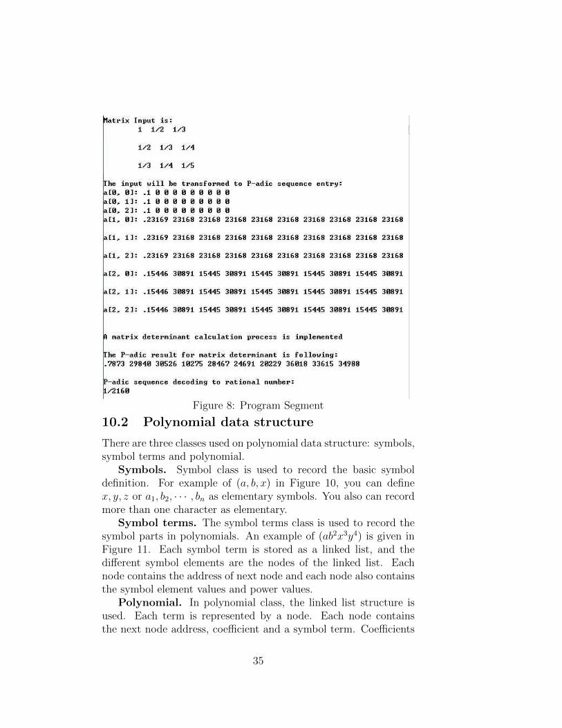
Figure 8: Program Segment

10.2 Polynomial data structure

There are three classes used on polynomial data structure: symbols,symbol terms and polynomial.

Symbols. Symbol class is used to record the basic symboldefinition. For example of (a, b, x) in Figure 10, you can definex, y, z or a1, b2, · · · , bn as elementary symbols. You also can recordmore than one character as elementary.

Symbol terms. The symbol terms class is used to record thesymbol parts in polynomials. An example of (ab2x3y4) is given inFigure 11. Each symbol term is stored as a linked list, and thedifferent symbol elements are the nodes of the linked list. Eachnode contains the address of next node and each node also containsthe symbol element values and power values.

Polynomial. In polynomial class, the linked list structure isused. Each term is represented by a node. Each node containsthe next node address, coefficient and a symbol term. Coefficients

35

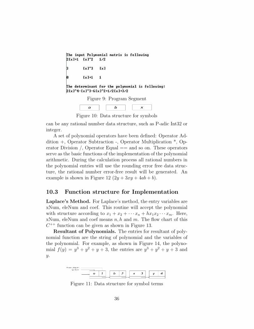
Figure 9: Program Segment

Figure 10: Data structure for symbols

can be any rational number data structure, such as P-adic Int32 orinteger.

A set of polynomial operators have been defined: Operator Ad-dition +, Operator Subtraction -, Operator Multiplication *, Op-erator Division /, Operator Equal == and so on. These operatorsserve as the basic functions of the implementation of the polynomialarithmetic. During the calculation process all rational numbers inthe polynomial entries will use the rounding error free data struc-ture, the rational number error-free result will be generated. Anexample is shown in Figure 12 (2y + 3xy + 4ab+ b).

10.3 Function structure for Implementation

Laplace’s Method. For Laplace’s method, the entry variables arexNum, eleNum and coef. This routine will accept the polynomialwith structure according to x1 + x2 + · · ·xn + hx1x2 · · · xm. Here,xNum, eleNum and coef means n, h and m. The flow chart of thisC++ function can be given as shown in Figure 13.

Resultant of Polynomials. The entries for resultant of poly-nomial function are the string of polynomial and the variables ofthe polynomial. For example, as shown in Figure 14, the polyno-mial f(y) = y3 + y2 + y + 3, the entries are y3 + y2 + y + 3 andy.

Figure 11: Data structure for symbol terms

36

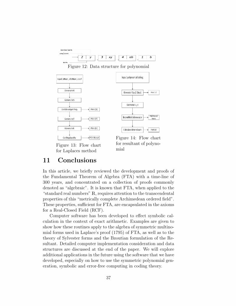
Figure 12: Data structure for polynomial

Figure 13: Flow chartfor Laplaces method

Figure 14: Flow chartfor resultant of polyno-mial

11 Conclusions

In this article, we briefly reviewed the development and proofs ofthe Fundamental Theorem of Algebra (FTA) with a time-line of300 years, and concentrated on a collection of proofs commonlydenoted as “algebraic”. It is known that FTA, when applied to the“standard real numbers”R, requires attention to the transcendentalproperties of this “metrically complete Archimedean ordered field”.These properties, sufficient for FTA, are encapsulated in the axiomsfor a Real-Closed Field (RCF).

Computer software has been developed to effect symbolic cal-culation in the context of exact arithmetic. Examples are given toshow how these routines apply to the algebra of symmetric multino-mial forms used in Laplace’s proof (1795) of FTA, as well as to thetheory of Sylvester forms and the Bzoutian formulation of the Re-sultant. Detailed computer implementation consideration and datastructures are discussed at the end of the paper. We will exploreadditional applications in the future using the software that we havedeveloped, especially on how to use the symmetric polynomial gen-eration, symbolic and error-free computing in coding theory.

37

Acknowledgment

This research project has been supported by the Air Force Officeof Scientific Research, FA9550-11-1-0315.

References

[1] Alperin, J.L., Local Representation Theory: Modular Repre-sentations as an Introduction to the Local Representation The-ory of Finite Groups, Cambridge University Press(1986)

[2] Arnold, B.H., A Topological Proof of the Fundamental Theo-rem of Algebra, Amer. Math. Monthly, 56, no.7(1949) 465-466

[3] Artin, E. & Schreier, O., Algebraische Konstruktion reellerKorper; Uber die Zerlegung definiter Funktionen in Quadrate;Eine Kennzeichnung der reell abgeschlossenen Korper, Abh.Math. Sem. Univ. Hamburg, 5(1927) 8599

[4] Bourbaki, N., Algebre, Chap. VI(1952), 40-41

[5] Branco de Oliveira, O.R., The Fundamental Theoremof Algebra: From the Four Basic Operations, arXiv:1110.0165v1(2011)

[6] Brown, W.C., Matrices Over Commutative Rings(1993), Mar-cel Dekker, New York

[7] Burkel, R.B., Fubinito Immediately implies FTA, Amer. MathMonthly 113(2006), 344-347

[8] Cauchy, A.-L., Cours d’analyse vol VII, Bologna(1990)

[9] Cayley, A., Note sur la methode d’elimination de Bezout, J.Reine Angew. Math 53(1857), 366367

[10] Dugundji, J., Topology, Allyn and Bacon(1966), New York

[11] Ebbinghaus et al, H.-D., Numbers, Graduate Texts in Mathe-matics vol. 123(1993), Springer-Verlag, New York

[12] Elliott, E.B., On the Existence of a Root of a Rational IntegralEquation, Proc. London Math. Soc.(1893) Series 1 25 173-184

38

[13] Fine, B. and Rosenberger, G., The Fundamental Theoremof Algebra, Undergraduate Texts in Mathematics, Springer-Verlag(1997), New York

[14] Foncenex, D. de, Reflexions sur les quantites imaginaires,Misc. Taurinensia 1(1759), 113-146

[15] Gauss, C.-F., Demonstratio nova theorematis functionem alge-braicam rationale . . . , Universitat Helmstedt(1799)

[16] Gauss, C.-F., Demonstratio nova alter theorematis onmenfunctionem algebraicam rationale integram . . . , Comm. Soc.Reg. Sci. Gottingen 3(1815), 107-142

[17] Gersten, S.M. and Stallings, J.R., On Gausss First Proof ofthe Fundamental Theorem of Algebra, Proc. Amer. Math.Soc(1988), 103 no. 1, 231-232

[18] Gordan, P., Ueber den Fundamentalsatz der Algebra, Math.Ann. 10(1876), 572-575

[19] Gordan, P., Vorlesungen ueber Invariantentheorie, vol 1(1885),B.G. Teubner, Leipzig

[20] Herstein, I.N., Topics in Algebra, second ed., J. Wiley(1975),New York

[21] Hille, E., Analytic Function Theory, Chelsea. 2 Vols(1973),New York

[22] Hyland, J.M.E., Why is there an Elementary Proof of the Fun-damental Theorem of Algebra?, Eureka 45(1985), 40-41

[23] Kerber, M., Division-free computation of subresultants usingBezout matrices. Tech. Report(2006) MPI-I-2006-1-006

[24] Lang, S., Algebra, 3rd revised ed. Springer-Verlag(2002), NewYork

[25] Littlewood, J.E., Mathematical notes (14): Every Polynomialhas a Root, J. London Mathematical Society 16(1941), 95-98

[26] Macdonald, I.G., Symmetric Functions and Hall Polynomials,2nd ed. Clarendon Press, Oxford(1998)

39

[27] Malet, J.C., Proof that every algebraic equation has a root,Trans. R. Irish Acad 26(1878), 453-455

[28] Mead, D.G., Newton’s Identities, The American MathematicalMonthly 99(1992), 749751

[29] Milnor, J., Analytic proofs of the ”hairy ball theorem” and theBrouwer fixed-point theorem, Amer. Math. Monthly 85(1978),no. 7, 521-524

[30] Smithies, F., A Forgotten Paper on the Fundamental Theoremof Algebra, Notes and Records of the Royal Society of London,54(2000) 333-341

[31] Stanley, R.P., Enumerative Combinatorics, Vol. 2. Camridge:Cambridge University Press, Cambridge(1999), U.K

[32] Stewart, I., Galois Theory, 3rd ed., Chapman andHall/CRC(2004), Boca Raton

[33] Sturm, C.-F., Memoire sur les resolutions des equationsnumeriques, Acad. Royale des Science 6(1835), 271-318

[34] Tarski, A., A Decision Method for Elementary Algebra andGeometry, Univ. of California Press(1951), Berkeley

[35] Taylor, P., Gauss’s Second Proof, Eureka 45(1985), 42-47

[36] Van der Waerden, B.L., Modern Algebra vol. 1, Ungar(1948),New York

[37] Wood, J. and Maskelyne, N., On the Roots of Equations,Philosophical Transactions of the Royal Society of London,88(1798), 369-377

40