FUNDAMENTAL STUDIES OF INTERFERENCES IN ICP - MS

FUNDAMENTAL STUDIES OF I N T E R F E R E N C E S IN

ICP - MS

By

LINDA K A T H L E E N R O W L E Y , BSc (Hons), MSc

A thesis submitted to the University of Plymouth

in partial fijlfilment for the degree of

DOCTOR O F PHILOSOPHY

Department of Environmental Sciences

Faculty of Science

In collaboration with

VG Elemental, Winsford, Cheshire

November 2000

90 0470386 4

U N I V E R S S T V O F P L Y M O U T H

Item No.

Date 1 1 J U L 2001 5

Class No" Cont. No

PLYMOUTH LiBRARY

LIBRARY S" ORF

ABSTRACT

FUNDAMENTAL STUDIES O F I N T E R F E R E N C E S IN ICP - MS

Linda Kathleen Rowley

Methods of temperature measurement by mass spectrometry have been critically

reviewed. It was concluded that the most appropriate method depended critically on the

availability of fundamental data, hence a database of fundamental spectroscopic

constants, for diatomic ions which cause interferences in ICP-MS, was compiled. The

equilibration temperature, calculated using the different methods and using various

diatomic ions as the thermometric probes, was between c.a. 400 - 10,000 K in the

central channel, and between c.a. 600 - 16,000 K when the plasma was moved 1.8 mm

off-centre. The wide range in temperature reflected the range of temperature

measurement methods and uncertainty in the fundamental data.

Optical studies using a fibre optic connected to a monochromalor were performed in

order to investigate the presence of interferences both in the plasma and the interface

region of the ICP-MS, and the influence of a shielded torch on these interferences. It was

possible to determine the presence of some species in the plasma, such as the strongly

bound metal oxides, however, no species other than OH were detected in the interface

region of the ICP-MS. The OH rotational temperature within the interface region of the

ICP-MS was calculated to be between 2,000 - 4,000 K.

The effect of sampling depth, operating power, radial position and solvent loading, with

and without the shielded torch, on the dissociation temperature of a variety of

polyatomic interferences was investigated. These calculated temperatures were then used

to elucidate the site of formation for different polyatomic interferences. Results

confirmed that strongly bound ions such as MO* were formed in the plasma, whereas

weakly bound ions such as ArO* were formed in the interface region due to gross

deviation of the calculated temperatures from those expected for a system in thermal

equilibrium.

CONTENTS

Title i

Abstract ii

Contents iii

List of Figures ix

List of Tables xv

List of Abbreviations xvii

Acknowledgements xxii

Authors Declaration xxiii

CHAPTER 1: INTRODUCTION I

1.1: General Introduction 2

1.1.1: History and Development of ICP - MS 2

1.1.2: The Inductively Coupled Plasma - Mass Spectrometer:

System Set - up and Operation 3

1.1.2.1: Forming and Sustaining the Plasma 6

1.1.2.2: Sample Introduction 7

1.1.2.3: Detection 11

1.1.3: Strengths and Weaknesses oflCP - MS 14

1.1.4: Applications of ICP - MS 17

1.2: Interferences in ICP - MS 18

1.2.1: Spectroscopic Interferences 18

1.2.1.1: Isobaric Interferences 18

1.2.1.2: Doubly Charged Species 20

1.2.1.3: Polyatomic Ion Interferences 21

iii

1.2.2: Methods for Removing Interferences 23

1.2.2.1: Multivariate Correction Methods 23

1.2.2.2: Alternative Sample Preparation Methods 24

1.2.2.3: Alternative Sample Introduction Methods 27

1.2.2.4: Instrumental Methods 29

1.2.3: Non-Spectroscopic Interferences 39

1.3: Fundamental Studies 41

1.3.1; Excitation Mechanisms 42

1.3.1.1: Formation Mechanisms of Analyte Ions 42

1.3.1.2: Formation Mechanisms of Molecular Ions 45

1.3.2: Ion Sampling and Formation of Secondary Discharge 47

1.3.2.1: Ion Sampling 47

1.3 .2.2: Formation of the Secondary Discharge 49

1.4: Aims of Study 51

CHAPTER 2: E X P E R I M E N T A L 52

2.1: Instnjmentation 53

2.1.1: PlasmaQuad 2+ ICP - MS 53

2.1.2: PlasmaQuad 3 ICP - MS 54

2.2: Reagent Preparation 56

CHAPTER 3: PRELIMINARY O P T I C A L STUDIES 57

3.1: Introduction 58

3.2: Experimental 58

3.2.1: Plasma Studies (Effect of Sampling Depth) 58

3.2.2: Interface Studies (Effect of Power) 62

3.3; Resuhs and Discussion 65

3.3.1: Plasma Studies (Effect of Sampling Depth) 65

3.3 .2: Interface Studies (Effect of Power) 73

3.3.2.1: OH Rotational Temperature 75

3.4: Conclusions 77

CHAPTER 4: C R I T I C A L COMPARISON O F T E M P E R A T U R E

DETERMINATION METHODS BY ICP - MS 79


4.1.1: lonisation Temperature 81

4.1.2: Dissociation Temperature 83


4.3: Results and Discussion 85

4.3.1: Radial Profile of ArX^ and MO' Species 85

4.3.2: Temperature Determination 90

4.3.2.1: Method A 90

4.3.2.2: Method B 94

4.3.2.3: Method C 98

4.3.2.4: Method D 105

4.3.2.5: Method E 108

4.4: Conclusions 111

4.4.1: Method A 111

4.4.2: Method B 112

4.4.3: Method C 112

4.4.4: Method D 113

4.4.5: Method E 114

4.4.6: Overall Conclusions 114

CHAPTER 5: E F F E C T O F SAMPLKSG DEPTH ON P O L Y A T O M I C

IONS AND T H E I R DISSOCL\TION T E M P E R A T U R E S 118




5.3 .1: Variation of Dissociation Temperature with Sampling

Depth 121

5.3.1.1: Dissociation Temperature of MO* 121

5.3.1.2: Dissociation Temperature of ArX* 127

5.3.2: Effect of Sampling Depth on M* Signal 129

5.3.3: Effect of Sampling Depth on MO" Signal 131

5.3 .4: Effect of Sampling Depth on ArX" Signal 136


CHAPTER 6: E F F E C T O F POWER ON P O L Y A T O M I C IONS AND

T H E I R DISSOCL\TION T E M P E R A T U R E S 146




6.3 .1: Variation of Dissociation Temperature with Power 148

6.3. M : Dissociation Temperature of MO" 148

6.3.1.2: Dissociation Temperature of ArX"^ 150

6.3 .2; Effect of Power on M* Signal 152

6.3.3: Effect of Power on MO* Signal 155

vi

6.3.4: Effect of Power on ArX^ Signal 159


CHAPTER 7: E F F E C T OF SOLVENT LOADIIVG ON POLYATOMIC

IONS AND T H E I R DISSOCL^TION T E M P E R A T U R E S 165




7.3 .1: Effect of Solvent Loading on Dissociation Temperature 169

7.3.2: Effect of Solvent Loading on Ion Signals 171


CHAPTER 8: DETERMINATION O F T H E SITE AND MECHANISMS O F

FORMATION O F P O L Y A T O M I C ION I N T E R F E R E N C E S 176




8.3.1: Temperature Determination 180


CHAPTER 9: CONCLUSIONS AND SUGGESTIONS FOR F U R T H E R

WORK 187


9.2: Suggestions for Further Work 191

References 193

Appendices 215

Appendix 1: Table of Fundamental Data 216

Appendix 2: Conferences and Courses Attended 219

Appendix 3: Presentations 221

Appendix 4: Publications 222

V l l l

LIST O F FIGURES

1.1 Schematic diagram of VG PlasmaQuad 3 ICP - MS instrumentation 4

1.2 Schematic diagram of a standard 'Tassel" ICP torch 5

1.3 Temperature regions of the ICP 7

1.4 ICP -MS sample introduction system 7

1.5 Concentric Meinhard nebuliser, showing enlarged nebuliser tip 8

1.6 Typical spray chamber designs. A: Scott double pass and B: single

pass with impact bead 9

1.7 Fate of a sample droplet af^er introduction into an ICP discharge 10

J.8 Two stage rotary pump ICP interface 11

1.9 Schematic of the supersonic expansion formed in the expansion chamber 13

1.10 Comparison of (A) standard inverted load coil system, and (B) centre -

tapped load coil system 33

M l Schematic diagram of the shielded torch system 33

1.12 Comparison of background spectra using standard plasma conditions

and shielded plasma conditions 34

3.1 Schematic diagram of the optical arrangement used to image the plasma

onto the tip of the fibre optic 60

3.2 Schematic diagram to show optical sampling of the plasma where the

plasma is moved to create a sampling depth profile 61

3.3 Schematic diagram to show optical sampling of the plasma where the

fibre optic is moved to create a sampling depth profile 62

3 .4 Schematic diagram of the fibre optic arrangement used to observe

the interface region of the ICP - MS 64

3.5 Schematic diagram of the tip of the fibre optic and spacer 64

3.6 Mass spectrometric sampling depth profile for Ti" within the plasma.

Errors = 3 a for n = 3 66

3.7 Optical sampling depth profile for Ti" within the plasma. Errors = 3 a

for n = 3 66

3.8 Mass spectrometric sampling depth profile for TiO^ within the plasma.


3.9 Optical sampling depth profile for TiO within the plasma. Errors = 3 a

for n = 3 69

3.10 Comparison of optical sampling depth profiles for TiO within the plasma,

at different sampling depth positions. Errors = 3 a for n = 3 72

3.11 Typical optical spectrum of OH (0 - 0) band emission showing Qi

branches 73

3.12 Effect of power on the signal for the Qi ' branch of the OH (0 - 0) band

emission at 307.844 nm within the interface. Errors = 3 a for n = 3 74

3.13 Comparison of the optical signal for the Hg reference line (546.07 nm)

through the interface and without the interface 74

3.14 Example of Boltzmann plot used to calculate the OH rotational

temperature within the interface 76

3.15 Effect of power on the OH rotational temperature within the interface

region of the ICP. Errors = 3 o for n = 3 77

4.1 Radial profile f o r ' '^In^ Errors = 3 a for n = 3 86

4.2 Radial profile for Ba^ Errors = 3 a for n = 3 87

4.3 Radial profile for Ba^'. Errors = 3 a for n = 3 87

4.4 Comparison of the radial profiles for MO^. Signals normalised to 100%

abundance (Signals divided by molecular abundance then multiplied by

100). Molecular abundances of the metal oxides are given in Table 4.1.

Do values given are for MO*. Errors = 3 a for n = 3 88

4.5 Radial profile for ArO" . Errors = 3 a for n = 3 89

4.6 Example of plot used to calculate the temperature using Method A 91

4.7 Comparison of the radial profiles for the temperature calculated using

Method A, with data for Do (MO) and Do (MO^. Errors = 3 a forn = 3 93

4.8 Example of plot used to calculate the temperature using Method B 96

4.9 Radial profile for the temperature calculated using Method B. Errors =

3 a for n = 3 97


Method C, with Do values for MO. Errors = 3 o for n = 3 102


Method C, with data for AlO and AlO*. Errors = 3 a for n = 3 104

4.12 Radial profile for the temperature calculated using Method D. Errors =

3 a for n = 3 106


Method E, for equilibration in the plasma and interface. Errors = 3 a for

n = 3 110


all methods. Errors = 3 a for n = 3 116

5.1 Schematic diagram of an ICP showing the different zones v^thin the

plasma 119

XI

5 .2 Comparison of the sampling depth profiles for the MO^ temperature.


5.3 Comparison of the sampling depth profiles for the MO" temperature

up to a sampling depth of 25 mm. Errors = 3 a for n = 3 123

5.4 Comparison of the sampling depth profiles for the ArO* temperature.

Errors = 3 a f o r n = 3 127

5.5 Sampling depth profile for Ba" . Errors = 3 o for n = 3 129

5.6 Sampling depth profile for BaO" . Errors = 3 a fiDr n = 3 132

5.7 Comparison of the sampling depth profiles for MO^ at 1350 W. Signals

normalised to 100% abundance. Molecular abundances of metal oxides

are given in Table 5.1. Do values given are for MO*. Errors =3 a for

n = 3 134

5 .8 Comparison of the sampling depth profiles for MO* with the shield torch

at 620 W. Signals normalised to 100% abundance. Molecular abundances

of metal oxides are given in Table 5.1. Do values given are for MO" .

Errors = 3 o f o r n = 3 135

5 .9 Comparison of the sampling depth profiles for MO* at 620 W. Signals

normalised to 100% abundance. Molecular abundances of metal oxides

are given in Table 5.1. Do values given are for MO*. Errors =3 a for

n = 3 135

5.10 Sampling depth profile for ArO*. Errors = 3 a fo rn = 3 136

5 .11 Comparison of the sampling depth profiles for the ArX* species at 1350W.

Signals normalised (Signals divided by highest signal in profile). Errors =

3 o f o r n = 3 138

M l

5.12 Comparison of the sampling depth profiles for the ArX^ species at 620W.

Signals normalised. Errors = 3 a for n = 3 138

5 .13 Comparison of the sampling depth profiles for the ArX^ species with the

shield torch at 620 W. Signals normalised. Errors = 3 o for n = 3 139

6.1 Comparison of the effect of power for the MO* temperature. Errors =

3 a f o r n = 3 149

6.2 Comparison of the effect of power for the ArO' temperature. Errors =

3 a f o r n = 3 151

6.3 Effect of power on the signal for La\ Errors = 3 a for n = 3 153

6.4 Effect of power on the signal for Al". Errors = 3 a for n = 3 154

6.5 Effect of power on the signal for LaO". Errors = 3 a for n = 3 156

6.6 Comparison of the effect of power for the MO" / M" ratio with standard

conditions. MO" and M^ signals normalised to 100%. Molecular and

atomic abundances are given in Table 6.1. Do values given are for MO* 157

6.7 Comparison of the effect of power for the MO* / M* ratio with the shield

torch. MO* and M^ signals normalised to 100%. Molecular and atomic

abundances are given in Table 6.1. Do values given are for MO* 157

6.8 Effect of power on the signal for ArO*. Errors = 3 a for n = 3 159

6.9 Comparison of the effect of power for the ArX*^ species with standard

conditions. Signals normalised. Errors = 3 a for n = 3 161

6.10 Comparison of the effect of power for the ArX* species with the shield

torch. Signals normalised. Errors = 3 a for n = 3 162

7.1 Schematic diagram of apparatus used for the introduction of water

vapour via a temperature controlled Dreschel bottle 167

X l l l

169

7.2 Effect of solvent loading for the ArO* temperature. Errors = 3 o for

n = 3

7.3 Effect of solvent loading for the ArX^ species at 1350 W. Signals

normalised. Errors - 3 a fo rn = 3 171

7.4 Effect of solvent loading for the ArX^ species at 700 W. Signals

normalised. Errors = 3 a for n = 3 174

7.5 Effect of solvent loading for the ArX* species with the shield torch.

Signals normalised. Errors = 3 a for n = 3 174

XIV

LIST OF TABLES

1.1 Detection limits (3o) for ICP - MS, ICP - AES and GF - AAS, for

selected elements 15

1.2 Examples of isobaric interferences encountered in ICP - MS 19

1.3 Commonly observed M " ions in ICP - MS and the affected isotopes 20

1.4 Common polyatomic interferences and the affected isotopes 22

1.5 Interferences of iron and selenium 23

2.1 ICP - MS operating parameters for PQ2+ 53

2.2 ICP - MS data collection parameters 54

2.3 ICP - MS operating parameters for PQ3 55

3.1 Operating conditions for the SPEX 1704 monochromator used for

optical observation of the plasma 59

3.2 Operating conditions for the SPEX 1704 monochromator used for

optical observation of the interface 63

3.3 Wavelengths of the Qi branches of the OH (0 - 0) band monitored

optically within the interface of the ICP 65

3.4 Assignment, wavelengths, energies and transition probabilities for the Qi

branches of the OH (0 - 0) band 77

4.1 Isotopes studied during radial profile experiment 85

4.2 Comparison of Do (MO) and Do (MO"^) values 92

4.3 Comparison of spectroscopic constants for AlO and AlO* 102

4.4 Comparison of the temperature calculated using all methods 115

5.1 Isotopes studied during effect of sampling depth experiment 121

6.1 Isotopes studied during effect of power experiment 148

7.1 Isotopes studied during the effect of solvent loading experiment 168

8.1 Isotopes studied during the introduction of 2% HNO3 for the site of

formation experiment 178

8.2 Isotopes studied during the introduction of 1% HCI for the site of


8.3 Isotopes studied during the introduction of 1% MeOH for the site of


8.4 Isotopes studied during the introduction of 10 ng ml'* MO solution for

the site of formation experiment 179

8.5 Dissociation temperatures calculated for the polyatomic ions (K) 182

LIST OF ABBREVIATIONS

a Degree of ionisation

AE Energy difference

Eoeb Nebuliser efficiency

A, Wavelength

a Standard deviation for 3 replicates

CO Vibrational constant

A Transition probability

AAS Atomic absorption spectrometry

AFS Atomic fluorescence spectrometry

Afm* Metastable excited argon atom

ArX Argon polyatomic molecule

ArX^ Argon polyatomic ion

B Rotational constant

BCR Community Bureau of Reference

C Solution concentration of indicated element

CCT Collision cell

CE Capillary electrophoresis

CID Collision induced dissociation

D Sampling diameter

dc / DC Direct current

dM Mass difference between peaks

Do Dissociation energy

DSI Direct sample introduction / insertion

E Energy

e" Electron

EIE Easily ionised element

ETV Electrothermal vaporisation

F Solution uptake rate

FIA Flow injection analysis

g Statistical weight of ground electronic state

GC Gas chromatography

GF - AAS Graphite furnace - atomic absorption spectrometry

h Plancks constant

HR - ICP - MS High resolution - inductively coupled plasma - mass spectrometry

hvcont Continuum photon

hvunc Spectral line photon

I Signal intensity

ICP Inductively coupled plasma

ICP - AES Inductively coupled plasma - atomic emission spectroscopy

ICP - MS Inductively coupled plasma - mass spectrometry

IE lonisation energy

IE' Second ionisation energy

INAA Instrument neutron activation analysis

IR Induction region

IRZ Initial radiation zone

k Boltzmann constant

K Equilibrium constant

Kd Equilibrium constant for dissociation of diatomic molecule

w i l l

KioD Equilibrium constant for ionisation of metal atom

K'ioo Equilibrium constant for ionisation of metal ion

LC Liquid chromatography

LTE Local thermodynamic equilibrium

M Mass

M Metal atom

Metal Ion

M"* Doubly charged metal ion

iMAr"*" Metal argide ion

MASSCAL Mass calibration solution

M H"*" Metal hydride ion

MIP Microwave induced plasma

M L R Multiple linear regression

MO Metal oxide molecule

MO"*" Metal oxide ion

MO / M Metal oxide to metal atom ratio

MO"*" / M* Metal oxide ion to metal ion ratio

IMO""] / IM""! Measured ratio of metal oxide ion to metal ion signal

M O I f Metal hydroxide ion

Mp Low energy (ground) state metal atom

Mp" Low energy (ground) state metal ion

Mq High energy state (excited) metal atom

Mq" High energy state (excited) metal ion

MS Mass spectrometry

m / z Mass to charge ratio

XIX

n Number density

NAZ Normal analytical zone

NdrYAG Neodymium - yttrium aluminium garnet

He- Number density of electrons

n.M Number density of metal atom

nM+ Number density of metal ion

n.Mo Number density of metal oxide molecule

no Number density of oxygen atom

No Avagadro's number

n\(pia una) Dcnsity of species X in plasma

nx(int) Density of species X in interface

p Vapour pressure

PGR Principle components regression

PII Polyatomic ion interference

PLS Partial least squares

p - LTE Partial local thermodynamic

ppb Parts per billion

ppt Parts per trillion

PS Plasma screen

Q Gas flow rate

R Universal gas constant

RF Radio frequency

Rp Resolution

RSD Relative standard deviation

SFC Supercritical fluid chromatography

XX

S I Spectroscopic interference

SsH Measured M* signal

SMO+ Measured MO' signal

S T Standard mode

T Temperature

T B Torchbox

TdL« Dissociation temperature

Te Electron temperature

Teic Excitation temperature

Tgas Gas kinetic temperature

Tion lonisation temperature

Tkin Kinetic temperature

Tpiasma Plasma temperature

Troom Room temperature

Trot Rotational temperature

Spray chamber temperature

X Position downstream from sampling orifice

X Metal or non - metal atom

X" Metal or non - metal ion

XRF X - ray fluorescence

XV^ Diatomic molecular ion

Z Partition function

XXI

ACKNOWLEDGEMENTS

I would like to offer my thanks to Dr Hywel Evans and Professor Les Ebdon for their

guidance and support throughout this PhD. I would also like to thank Professor Steve

Hill for the loan of the monochromator.

I would like to thank the EPSRC and VG Elemental for a CASE research grant, and

providing the spare expansion chamber which was modified for the optical measurements

in the interface, and to my industrial supervisor Dr Martin Liezers.

Thanks to everyone I have worked with during my time in Plymouth, past and present,

including Fishcake, Gav, Neil, Wobbly Bob, Elena, Jason, Anita, various mad Spaniards

(with varying degrees of madness!), Matt, Hugh, Warren, Jackie and anyone else I've

forgotten to mention. Special thanks to James who, even though he*s in America, found

the time to proof read my thesis - Cheers Scouse!!!. Further special thanks to Rob

Harvey who was just down the corridor whenever Gordon or Thomas *'went bang"!!!

Extra special thanks to Rob for putting up with me throughout the PhD and the writing

of this thesis - 1 told you I 'd get it done eventually!!

Finally, I would like to dedicate this work to my parents, who have been there all

through my student life providing constant support in the form of both finance and food

parcels, to Grandma and to the memory of my other grandparents. I hope I've done you

proud.

XXII

AUTHORS DECLARATION

At no time during the registration for the degree of Doctor of Philosophy has the author

been registered for any other University award.

The study was financed with the aid of a CASE studentship from the Engineering and

Physical Sciences Research Council in collaboration with VG Elemental, Winsford,

Cheshire.

The work described in this thesis has entirely been carried out by the author. Relevant

scientific seminars and conferences were regularly attended at which work was

presented, external institutions were visited for consultation purposes, and several papers

were prepared for publication.

Signed. >?d^%^^

\\\\\

CHAPTER 1

Introduction

1 INTRODUCTION

1.1 GENERAL INTRODUCTION

1.1,1 History and Development o f l C P - MS

The need for ultra - trace level elemental analysis has been a major driving force

for the development and improvement of analytical techniques. Plasma source mass

spectrometry is one technique that is currently of interest for multi - element analysis at

the part per billion (ppb) and part per trillion (ppt) levels*.

The original concept of ICP - MS developed from a requirement, expressed in

1970, for the next generation of multi - element analytical instrument systems needed to

complement the rapidly developing technique of ICP - AES^ which suffered from a

number of matrix interferences^. Following a survey of available and emerging

techniques, including atomic fluorescence spectrometry (AFS), instrumental neutron

activation analysis (FNAA), atomic absorption spectrometry (AAS) and X - ray

fluorescence (XRF), it was concluded that atomic mass spectrometry was the only basic

spectrometric technique that potentially had the wide element coverage, element

specificity and relatively uniform sensitivity across the Periodic Table that was essential.

The ICP operating at atmospheric pressure was first utilised by Reed** in 1961 to

grow crystals under high temperature conditions. The analytical potential of the ICP as

an optical source was realised by Greenfield et al.^ in 1964 and Wendt and Fassel in

1965. Initial work on plasma MS was carried out by Gray^ '**, who used a small direct

current (dc) plasma, which was being used for emission studies, as an ion source for

mass spectrometry. However, the ionisation temperature was too low to provide

adequate ionisation of elements whose ionisation energy was greater than about 8 eV,

and severe ionisation suppression was caused by easily ionised elements (EIEs)**. This

ultimately led to the replacement of the capillary dc arc by an ICP by Gray and Houk'^,

whereas Douglas^^ at the University of Toronto began work with a microwave induced

plasma (MIP).

The first paper describing the coupling of an argon plasma and a mass

spectrometer was published in 1980 by Houk <?/ a/.'^, as a result of the collaboration

between the research group at the Ames Lab, Iowa State University and Gray at the

University of Surrey. Work was also underway by Douglas and colleagues''* at Sciex in

Canada. The first mass spectra from an ICP source were obtained by Date and Gray*^ '*'

in 1982. By 1983 two commercial instruments were launched, the PlasmaQuad, based on

the Surrey system, by VG Isotopes Ltd. (now T J A Solutions) in the U K ' \ and the Elan

in Canada by Sciex Inc. (now Perkin Elmer Ltd.), based on the work of the Toronto

group^^. Since this time ICP - MS has experienced rapid growth and there are now at

least six manufacturers, with the original quadrupole ICP - MS being continuously

modified. Many features, such as the shield torch system*^ and collision cell

technology* * **, have also been introduced to overcome interferences. In addition to the

original quadrupole ICP - MS some manufacturers also produce a high resolution

magnetic sector ICP - MS. A schematic diagram of a typical quadrupole ICP - MS is

given in Figure 1.1.

1.1.2 Inductively Coupled Plasma - Mass Spectrometer: System Set - up and

Operation

The ICP is an electrode - less discharge in a gas at atmospheric pressure,

maintained by energy coupled to it from a radio frequency generator. The gas used is

commonly argon, although other gases, such as nitrogen and helium, have been used^V

Quadrupole ^^^^^^ mass filter

Detector

P C

Jl

Skimmer cone

ampling cone

Torch

Analyser Stage

Plasma

Expansion Stage

Interm ediate Stage

F T * Spary Chamber

Nebuliser

Peristaltic Pump

Sample

Figure 1.1: Schematic diagram of VG PlasmaQuad 3 ICP- MS instrumentation'

The plasma is generated inside and at the end of an assembly of quartz tubes

known as the torch. The standard Fassel type torch is shown in Figure 1.2.

Induction Coil

Injector Tube

Concentric Quarto Tubes

X

V ^ Aerosol of Ar

sample 0.5-1.5lmln-^

Coolant Gas Auxiliary Gas 10-15lmin-' ' 0 -3 lmln-^

Figure 1.2: Schematic diagram of a standard "Fassel" ICP torch

This consists of an outer tube within which are two concentric tubes terminating short of

the torch mouth. Each annular region formed by the tubes is supplied with gas by a side

tube entering tangentially, so that it creates a vorticular flow. The innermost of the three

gas flows (the nebuliser or injector gas) carries the aerosol from the sample introduction

system at about 1.0 1 min"'. This produces a high velocity jet of gas which punches a hole

in the base of the plasma. This central, or axial, tunnel is cooler than the rest of the

plasma, but at 5000 - 6000 K is hot enough to atomise most samples and cause varying

degrees of ionisation of the constituent elements^. The outer, or coolant, gas flow

(usually 10-151 min'') protects the torch walls and acts as the main plasma support gas.

The second, or auxiliary, gas flow (0 - 1.5 I min'*) ensures that the hot plasma is kept

clear of the tip of the injector tube.

/ . / . 2.1 Forming and Sustaining the Plasma

Upon emerging at the tip of the torch the argon gas is surrounded by a 2 or 3 -

turn water cooled copper induction coil, which is located with its outer turn about 5 mm

below the mouth of the torch. An alternating current flows through this coil, typically at

a frequency of either 27.12 or 40.68 MHz and power levels of I - 3 kW^^ The argon gas

stream that enters the coil is initially seeded with free electrons from a Tesia discharge

coil. These seed electrons quickly interact with the magnetic field of the coil and gain

sufficient energy to ionise argon atoms by collisional excitation. Cations and electrons

generated by the initial TesIa spark are accelerated by the magnetic field in a circular

flow perpendicular to the stream that emerges from the tip of the torch. The fast moving

cations and electrons, known as an eddy current, collide with more argon atoms to

produce ftirther ionisation and intense thermal energy. This collisional ionisation

continues in an "avalanche" reaction forming the ICP discharge.

The ICP is sustained by continuous energy transfer between the radio frequency

(RF) generator and the torch. A flame shaped plasma is formed near the top of the torch,

with a temperature of 6000 - 10,000 K ^ , although the degree of ionisation of argon is

only about 0.1 % at these temperatures^^ The temperature distribution throughout the

system is shown in Figure 1.3.

A plasma with torroidal, or annular, geometry results from the aerosol gas

punching the plasma, which lengthens the residence time (approx. 2 ms) of the sample in

the interior, high temperature zone of the plasma, thereby increasing sensitivity for many

elements. The sample stream then forms a long, well defined tail emerging from the high

temperature region v^thin the load coil. This tail is the spectroscopic source, containing

all the analyte atoms and ions that have been excited and ionised.

Temperature (K) (t10%)

6500K

eoooK BOOOK

G O O

r z 1

6200K eeoQK

o o o

10.000K

Figure 1.3: Temperature regions of the ICP

I. L 2.2 Sample Introduction

There are a number of different ways that samples can be introduced to an ICP,

but the most common method is by aspiration of aqueous samples. The sample

introduction system for simple aqueous samples consists of a peristaltic pump, a

nebuliser, a spray chamber and a torch, and this set - up is shown in Figure 1.4.

MASS R O W

COHTROOBl

WATWOUT - * WASTE WATER COOLED

SPRAY CHAMBER

Figure 1.4: ICP - MS sample introduction system

The sample is pumped via a peristaltic pump to a nebuliser, normally a

pneumatic ** or ultrasonic nebuliser^', where it comes into contact with argon gas,

regulated by a mass flow controller, generating an aerosol. The pneumatic method, in

which a high velocity gas stream produces a fine droplet dispersion of the analyte

solution, is the most popular because of its convenience, reasonable stability and ease of

use. Various pneumatic nebuliser designs exist and include the concentric glass

nebulisers, such as the Meinhard, shown in Figure 1.5, cross flow nebulisers, and V -

groove nebulisers.

A R G O N

^ S A M P L E

Figure L5: Concentric Meinhard nebuliser, showing enlarged nebuliser tip

However, other techniques are also becoming more widely used, with liquid

sample introduction being achieved using ultrasonic nebulisers"'^°, thermospray

vaporisers ' ' ^ and direct injection nebulisers'*"*"** which can improve nebulisation and

transport efficiencies.

33-35

Liquid samples, either aqueous or organic, have also been introduced into the

plasma using chromatographic techniques, including liquid chromatography (LCf^^^'^^

42 , gas chromatography (GC) 36,37,39,43 , flow injection analysis (FIA)'""^^ supercritical fluid

,50.52 chromatography (SFC/ ' '*'*' ' and capillary electrophoresis (CE)'

Gaseous sample introduction into the ICP offers several advantages over liquid

sample introduction. Unlike pneumatic nebulisation, where > 90 % of the sample is

discarded using most nebulisation systems, the transport efificiency of a gas to the plasma

approaches 100 %. Thus, more sample reaches the plasma, resulting in improved signal -

to - background ratios and detection limits. The introduction of gaseous samples to the

ICP has been performed using hydride generation^^ and direct injection '*.

The analysis of solid samples employs either vaporisation of the sample, i.e.

electrothermal vaporisation (ETV)'^"^* or laser ablation""****, or direct analysis, i.e. slurry

65-67 nebulisation

After the aerosol has been formed it must be transported, via a spray chamber, to

the torch for introduction to the plasma. Figure 1.6 shows some typical spray chamber

designs.

TO ICP

WATER OUT,

DRAIN WATER IN

A: Scott Double Pass B: Single pass with impact bead

Figure 1.6: Typical spray chamber designs. A: Scott double pass and B: single pass

with impact bead

The spray chamber is placed between the nebuliser and the torch and serves to

remove the large aerosol droplets and to smooth out pulses occurring during nebulisation

due to pumping of the solution. Only droplets less than about 10 |im reach the plasma

after passing through the spray chamber, which constitutes about I - 2 % of the sample

that is introduced to a pneumatic nebuliser . For an ultrasonic nebuliser the percentage

efficiency is significantly greater. The spray chamber is required because these larger

droplets would cause signal fluctuations, plasma instability and eventually could

extinguish the plasma.

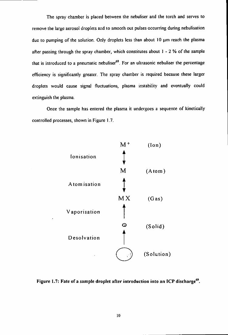
Once the sample has entered the plasma it undergoes a sequence of kinetically

controlled processes, shown in Figure 1.7.

( Ion)

lonisation •

I M (Atoin)

Atom isation

Vapor i sa t ion

Deso lvat ion

M X (Gas) a

^ ( S o l i d ) A

(So lut ion)

Figure 1.7: Fate of a sample droplet after introduction into an ICP d^scharge^^

10

A droplet of sample undergoes desolvation until a dry or nearly dry particle remains. The

particle is heated by the plasma, and vaporisation begins when the particle surface

temperature is sufficiently hot. Molecules or atoms are released into the plasma at rates

that depend on either the transfer of heat to the particle surface, or the transfer of

vaporised sample away from the particle surface . Molecules are atomised and atoms are

ionised in the plasma, and the vaporisation products diffuse. The ions produced in the

ICP are then transported through the sampling orifice, skimmer, ion optics, the mass

spectrometer and then strike the ICP - MS detector.

IJ.2.3 Detection

The use of an ICP as an ion source for mass spectrometry has several intrinsic

problems because the plasma operates at atmospheric pressure while the mass

spectrometer operates under high vacuum. This extraction is achieved using a two stage

rotary pumped interface, shown in Figure .1.8.

Slide Vatve

Skimmer Cone

Sampler Cone

Extraction Lens

Figure 1.8: Two stage rotary pump ICP interface

11

The interface consists of two nickel or platinum cones enclosing a region of

intermediate pressure between the plasma and mass spectrometer. The ions are extracted

through a 1 mm sampling cone into a low pressure expansion chamber. As the gas

emerges through the sampling orifice it undergoes rapid adiabatic expansion, where the

kinetic temperature of the gas falls but the total enthalpy remains constant, and the flow

becomes supersonic. Under these conditions, the kinetic energy of the sample is

converted into a directed flow along this axis. In effect, a free jet is formed that is

bounded by a shock wave known as ''barrel shock". The barrel shock helps prevent the

gas jet from mixing with any surrounding gas and hence helps prevent the formation of

molecular species. A second shock wave exists across this axis. This is formed when the

expansion is halted by the background gas pressure. This second shock wave is called the

Mach disc. The position of the Mach disc is dependent on the diameter of the aperture in

the sampling cone and on the pressure, and is typically 10 mm behind the aperture.

Behind the Mach disc the ion beam becomes subsonic again and may mix with any

surrounding gas. To prevent this a skimmer cone is placed at a distance of just over 6

mm away from the aperture of the sampling cone, as shown in Figure 1.9. This allows

the gas jet to pass through to the next stage of the spectrometer. Once through the

skimmer, the gas jet becomes random and requires focusing onto the detector by a set of

electrostatic ion lenses.

The function of the ion lenses is to focus as many ions as possible from the cloud

formed behind the skimmer cone through a differential pumping aperture into an axial

beam of circular cross section at the entrance to the quadrupole mass analyser. The ion

lenses are basically metal rings with electric potentials applied to them, and are housed in

the intermediate region of the instrument. Several different systems are in use, and many

have a photon stop present on the axis to prevent photons from the plasma reaching the

detector and adding to the background signal.

12

S k i m m e r Barre s h o c k

Mach disk

Figure 1.9: Schematic of the supersonic expansion formed in the expansion

chamber

The function of the quadrupole is to produce an electric field that selectively

allows a stable trajectory for ions that have a narrow mass - to - charge ratio (m / z). It is

comprised of four electrically conducting rods that are arranged to produce an oscillating

electric field between them. Before the main mass analyser there is often a series of pre -

rods which are used to improve the transmission of the lighter ions and to prevent

contamination of the main analyser. Similarly, at the end of the main analyser a set of

rods can be used to improve extraction of the ions. The entire assembly is under high

vacuum to ensure that there is no residual gas that can disrupt the ion trajectories by

scattering, and hence causing decreased sensitivity. The ions of selected m / z

"corkscrew" their way through the filter while other ions strike the rods and are lost.

The ions transmitted fi-om the quadrupole mass analyser are detected by an

electron multiplier. In a single dynode multiplier a positive ion strikes the funnel of the

multiplier to produce one or more secondary electrons which are ejected from the

13

surface and accelerated down the tube. During the passage down the tube they collide

with the walls dislodging fijrther electrons and thus an avalanche effect quickly builds up.

At the bottom of the tube the cloud of electrons leave the base of the channel and is

attracted by a collector electrode. The signal is therefore measured as an electrical pulse,

which is transferred to a computer. Once stored on the computer the data can be

manipulated as appropriate.

1.1.3 Strengths and Weaknesses of ICP - MS

ICP - MS has both a number of advantages over its rival techniques, but also

some disadvantages. The coupling of the highly efficient ICP ion source with the

sensitivity and selectivity of the mass spectrometer means that the ICP - MS is a highly

sensitive instrument, with detection limits in the sub ppt range, although these are usually

obtained under ideal conditions using ultra pure deionised water. These detection limits

are, for most elements, at least three orders of magnitude better than ICP - AES and

better than, or equivalent to, detection limits obtainable with GF - AAS. Some examples

of this are summarised in Table 1.1 In addition to being sensitive the technique has a

linear calibration range of at least six orders of magnitude, which is far superior to that

obtainable with GF - AAS. Another key advantage of the ICP - MS is the semi -

quantitative capability. This allows the operator to measure the concentration of over 60

elements, in under sixty seconds, to within a factor of 2 or 3 of the true value. Another

feature of the quadrupole mass spectrometer is multi - element analysis, with the

possibility of fully quantitative calibrations for elements across the mass range. ICP -

AES also offers a multi - element facility, but this is limited by the monochromator or the

polychromator used. GF - AAS is typically a single element technique and as a result the

sample throughput is far lower than for the ICP techniques.

14

Table l . l : Detection limits (3a) for ICP - MS'^ ICP - AES'^ and G F - AAS'^ for

selected elements.

Element ICP - MS (ppt)" ICP - AES (ppb)** G F - A A S (ppb)**

Li 0.01 -0.1 (PS) 1 0.1

B 10- 100 (ST) 0.5 43

Na 0.1-1 (PS) 1.0 0.05

S >1000 (ST) 20 -

Ca 1 - 10 (PS) 0.03 0.04

Mn 0.1 - 1 (ST/PS) 0.3 0.03

Fe 0.1-1 (PS) 1 0.06

Ni 0.1 - 1 (PS) 6 0.24

Co 0.1 - 1 (ST) 2 0.5

Cu 0.1-1 ( P S / C C T ) 2 0.07

Zn 0.1 - I (PS) 1 0.008

As 1 - 10 (ST/CCT) 12 0.33

Rb 0.01 -0.1 (ST) 35 0.06

Mo 0.01 -0.1 (ST) 4 0.14

Cd 0.01 -0.1 (ST) 1 0.02

Te 1 - 10 (ST) 27 0.5

La 0.01 -0.1 (ST) 0.02 -

Lu 0.01 -0.1 (ST) 0.05 -

Au 0.01 -0.1 (ST) 0.5 0.05

Hg 1 - 10(ST) 9 18

Pb 0.01 -0.1 (ST) 14 0.04

U 0.01 -0.1 (ST) 3.5 -

a) ICP - MS data obtained in multi - element mode with 10 s integrations, data from TJA

Solutions product literature*^ (ST = standard mode, PS = plasma screen, CCT = collision

cell)

b) ICP - AES data and GF - AAS data represent the technique, not a particular

instrument'**

15

Most instruments have single - ion monitoring and time - resolved analysis. These

are software packages that monitor the signal at one isotope for single - ion monitoring

or at several isotopes in a rapid sequential manner for time - resolved analysis. They are

most useful with transient signals, such as those obtained with laser ablation, flow

injection, electrothermal vaporisation, or when chromatography is being coupled with

ICP - MS. Another advantage is that the ICP - MS can be used to determine isotope

ratios for geological, or other applications, and isotope dilution analysis.

The ICP - MS is extremely flexible with respect to sample introduction, being

able to admit samples as gas, liquid or solid. Manufacturers offer laser ablation and

electrothermal vaporisation (ETV) accessories for solid sample introduction and hydride

generators for gaseous sample introduction into the ICP - MS. These options are also

available for ICP - AES but have been less extensively exploited commercially. GF -

AAS can take samples as liquid or solid, but sample loading is time consuming and

awkward.

While ICP - MS has a number of distinct advantages over competitive techniques

it has some notable drawbacks. Firstly, it is expensive both to purchase and maintain,

with instruments costing > £100 K and accessories up to £20 K, while the running costs

amount to about £5 K per annum. This is some two to three times and five to seven

times the cost incurred in buying and running an ICP - AES and GF - AAS instrument

respectively. In addition to these costs an ICP - MS instrument should ideally be kept in

a temperature controlled clean room in order to function at its best, which can be

expensive. The biggest problem encountered in ICP - MS is the occurrence of

interferences, which is discussed in Section 1.2.

16

1.1.4 Applications of ICP - MS

The advantages of ICP - MS over competitive techniques has resulted in its rapid

application in a wide range of fields. ICP - MS is now used in many areas including:

• Clinica^'"'^ i.e. analysis of body fluids for toxic metal levels or for vital trace

elements.

• Biological **' ', i.e. analysis of animal or plant materials, or sediments for toxic metal

levels.

• Geo!ogical^^''\ i.e. analysis of potential ore materials or isotopic ratio measurements

for dating rocks.

• Nuclear industry '** ^ where the sensitivity and speed of analysis make it more

favourable than traditional techniques for the analysis of radioactive materials or

dosimetry of nuclear industry workers.

• Water industry^ ' , where high sample throughput and multi - element capabilities

make it well suited to the analysis of potable waters.

• Chemicals and petroleum industries"*'******"'****, for both routine and more specialised

applications, i.e. ultratrace analysis of high purity chemicals or analysis of impurities in

materials, such as steel.

• Environmental*** '** , i.e. analysis of environmentally sensitive elements such as Cd,

As or Pb.

• Certification and validation**' * **, i.e. Certification of Community Bureau of

Reference (BCR) reference materials (now the Measurements and Testing

Programme).

• Higher education establishments, for both fijndamental and applied research.

17

1.2 I N T E R F E R E N C E S IN ICP - MS

Interferences which occur in ICP - MS can be defined as either spectroscopic or

non - spectroscopic. Spectroscopic interferences are caused by atomic or molecular ions

having the same nominal mass as the analyte of interest, thereby interfering with the

analysis by causing an erroneously large signal at the m / z of interest* *. Non -

spectroscopic interferences (or matrix effects) are complex, not specific to one particular

element and not apparent in the spectrum. They can be divided into* *:

a) suppression and enhancement effects,

b) physical effects caused by high total dissolved solids.

1.2.1 Spectroscopic Interferences

Spectroscopic interferences (Sis) can be divided into 3 main areas' *;

a) isobaric overlap,

b) doubly charged ions,

c) polyatomic ion interferences.

L 2. L1 Isobaric Interferences

Isobaric interferences occur when two or more elements have isotopes at the

same nominal mass. In fact, masses may differ by a small amount (0.005 m / z) which

cannot be resolved by a conventional quadrupole mass analyser. Some examples of these

isobaric interferences are shown in Table 1.2. Isobaric overlaps are well documented, and

hence easy to predict, and can be overcome by the use of elemental equations* '' ^

However, in practice, isobaric interferences are not always a problem because all

18

elements, with the exception of In at m / z 113 and 115 (which overiap with "^Cd and

"^Sn), have at least one isotope which is free from isobaric overiap

Table 1.2: Examples of isobaric interferences encountered in ICP - MS

Isotope Isobaric Interference

•'S (0 02) "'Ar (0 34)

** K (0 01) •*'Ar (99 6) &-^^Ca (96 9)

^ V (0 25) ^^Ti (5 30) & ^'Cr (4 35)

•*Ni (0 95) '•*Zn (48 9)

' 'Sr(0 56) ' 'Kr(57 0)

^'Zr(17 1) ^^Mo(14 8)

"Mn (4 3) ' ' 'Cd(12.2)

"-In (95 7) '"Sn(0 35)

'-'Te (4 60) '^'Sn (5 8) & '^'Xe (0 01)

"*Nd(5 7) "'^Smdl 2)

'^Gd (21 7) '^^Dy(2 30)

''^Lu (2.6) ' ' 'Yb(12.7)& " ' H f ( 5 20)

'"^Pt (25 3) ""Hg (0 15)

^ > b ( l 4) ' ' 'Hg (6 8)

Values in brackets are isotopic abundances

1'^

1.2. L 2 Doubly Charged Species

Doubly charged ions (M^^ are common for elements with a low second

ionisation potential, such as barium, which has a second ionisation potential of 10.0 eV.

The alkaline earth elements, the rare earth elements and elements such as U and Th are

most likely to form M " species. The formation of a doubly charged ion results in a loss

of sensitivity for the singly charged species and also generates an isotopic overiap at one

half of the mass of the parent element. The problem of M " formation is fijrther

exacerbated if the interferent precursor is present in high concentrations, which is of en

the case with the rare earth elements in geological samples* . The range of M^*

interferences is shown in Table 1.3.

Table 1.3: Commonly observed IM'" ions in ICP - MS and the afTected isotopes

M^* Species Affected Isotope

''Ca (2.06)

''Ga (60.2)

'**Ge (20.5)

''Se (7.58)

** Rb (72.2)

''Sr (82.5)

**^Sn(14.2)

238y2+ ** Sn (8.58)

Values in brackets are isotopic abundances.

20

7.2.1,3 Polyatomic Ion Interferences

This form of spectroscopic interferences is far more of a problem than isobaric

interferences and can be much more difficult to overcome. Polyatomic ions are molecular

species which are formed in the plasma and interface region of the ICP - MS. These

polyatomic ions typically come fi-om precursors in the argon support gas (e.g. Ar, H, O),

entrained atmospheric gases (e.g. N, O), from solvents or acids used during sample

preparation (e.g. N, CI, S, P), or from the sample matrix, and are particularly problematic

below m / z go* ** ' ^*". Polyatomic ion intereferences (PDs) can be placed into several

groupings;

* oxides i.e. ArO\ C\0\ MO'

* hydroxides i.e. ArOPT, ClOH", MOIT

* hydrides i.e. ArH*, MH'

* argides i.e. MAr'.

Therefore, their occurrence will depend on the sample composition with regard

to both the solute and the solvent. Common examples of polyatomic ion interferences are

given in Table 1.4, although this is by no means an exhaustive list. Particularly

problematic polyatomic interferences are those which interfere with mono - isotopic

elements, i.e. ^^ArCr on ' As" and *** ArCu* on *' Rh' . Other problematic elements are

Fe and Se, as they suffer from interferences on most of their isotopes, as shown in Table

1.5.

21

Table 1.4: Common polyatomic interferences and the affected isotopes

Polyatomic interference AfTected Isotope

"0 (0.20)

^'Si (92.2)

"NOPT "P(IOO)

"S (95.0)

•"N20*, •"C02" •"Ca (2.08)

"Cr (83.8)

"Fe (2.36)

'*Fe (91.7)

"ArOir "Fe (2.14)

**ArCO* '"'Zn(18.6)

"ArCr ''As (100)

'*Ar2^ "Se (7.7)

»"Ar2 '"Se (50.0)

'"^ArCu* '"Rh(lOO)

'"BaO^ '"Sm (22.8) & '"Gd (2.2)

"»BaOH^ '"Gd(14.9)

'»'HoO^ "'Ta (99.9)

"'Os(41.0)& ' 'Pt (0.78)

Values in brackets are natural isotopic abundances

* Radioactive isotopes

22

Table 1.5: Interferences of iron and selenium

AfTected Isotope Interferent Ion

"Fe (5.8) '"Cr (2.36) & "ArN

' Fe (91.7) ^^ArO

"Fe (2 .14) "ArOH

''Fe (0.31) 'Ni (67.8)

''Se (0.9) ''Ge (36.4)

' Se (9.0) '**Ge (7.7)&'*'Ar2

"Se (7.5) "ArCl

''Se (23.5) ''Kr (0.35)&''Ar2

'**Se (50.0) '**Kr (2.25) &'**Ar2

''Se (9.0) ''Kr(11.6)

Values in brackets are isotopic abundances

1.2.2 Methods for Removing Interferences

The problem of spectroscopic interferences can be dealt with in two ways, either

by their removal or by correcting for them. Careful setting of instrumental parameters

has been shown to reduce the relative levels of interferences'' ** '*** ^ with the nebuliser

gas flow, sampling depth and forward power being the most important.

1.2,2.1 Multivariate Correction Methods

One of the simplest methods to correct for spectroscopic interferences is the use

of mathematical correction methods* ''*'**'* ***"'*", such as elemental equations* "*'**'* *

and multivariate techniques*"'*". Elemental equations* '*'**'* * have been used to correct

for both isobaric and polyatomic interferences. For example, the interference caused by

23

•^^Ar^cr on ' As^ can be corrected for by measuring the ''W^Cr signal at m / z 77 and

back calculating the contribution fi-om **°Ar"cr at m / z 75, assuming the sample does

not contain "Se^ ' V

Multivariate techniques used to overcome spectroscopic interferences include

multiple linear regression (MLR)*", principle components regression (PCR)'" and

partial least squares (PLS)'". MLR and PCR have been used to correct for MoO^, ZrO"

and RuO* in the determination of low levels of C d \ In^ and Sn , respectively PLS has

been used to correct for interferences caused by light rare earth oxides on heavier rare

earth elements*".

L 2.2.2 A hern ative Sample Preparation Meth ads

a) Sample Dissolution Procedures

Polyatomic interferences can be removed by alternative sample preparation,

which may be as simple as changing the dissolution media in order to remove the

interference precursors fi-om the plasma system. Hence, if V or As is to be determined

then hydrochloric acid should be avoided in order to prevent the occurrence of CI based

polyatomic interferences. In general, nitric acid is favoured as a dissolution media as it

gives rise to the simplest spectra, with digestion media such as hydrochloric, sulphuric

and phosphoric acids all giving rise to a wide range of

interferences* *' '* '*'*'''*"'*'''* •* •**' However, it is not always possible to use an

alternative sample digestion media, particularly for geological samples* **. One answer to

this problem has been the use of slurry nebulisation "** , where the sample is introduced

as a finely ground solid in suspension, avoiding the need for sample dissolution.

While it is possible to avoid potential interferences due to acids used for

dissolution, if the sample matrix itself contains the interfering species then it is often

necessary to separate the analyte completely from the interfering matrix component.

24

h) Desolvation Techniques

Many of the most serious polyatomic interferences in ICP - MS are caused by

species which contain oxygen in combination with an element in the support gas (e.g.

argon or nitrogen), in the acids used to dissolve the sample (e.g. chlorine or sulphur), or

in the sample itself ** *^^*". Since water is the major source of oxygen in the plasma when

nebulising aqueous samples, decreasing the water loading decreases the oxygen

concentration in the plasma^ '* .

An extremely simple method to reduce oxygen - containing interferences derived

from injected water is to cool the spray chamber, thereby condensing some of the water

vapour. More efficient solvent removal can be achieved by the use of more complex

arrangements, such as Peltier coolers*", membrane interfaces^^''^, or heater /

condensers ' **. These methods have reduced the levels of both oxides and polyatomic

ion interferences, while increasing the sensitivity for a variety of metal analytes.

The desolvation system generally used with an ultrasonic or thermospray

nebuliser can also be used with other nebulisers for attenuating polyatomic ions

containing oxygen. The aerosol is first heated to vaporise the solvent. Most of the

solvent vapour is then removed in a condenser that is kept at a temperature near the

melting point of the solvent, i.e. 0 - 2 °C for water*^. Additional water may be removed

by attaching a second device to the outlet of the condenser.

Cryogenic desolvation uses repetitive heating and cooling steps to condense

solvent vapour **'' ' " . In this method the aerosol generated by the nebuliser is heated to

140 °C and then passed through a series of condensers. The first condenser at 0 °C

removes most of the water present. The partially dried aerosol stream is warmed to room

temperature before it enters a second glass condenser at - 80 °C. The aerosol stream then

25

passes into a set of copper loops where it is repeatedly cooled and heated at - 80 °C and

140 °C respectively, before being transported to the ICP **.

Membrane methods also vaporise the solvent, which then passes as a vapour

through a porous membrane and is evacuated or purged continuously by a sweep

g^g28.29.i6o,i6i,i64 ^ ^ ^ j ^ j _ ^ ^ ^ ^ j Nafion® dryer, located between the spray chamber and

torch, has been used to remove 97 % of the total mass of water leaving the spray

chamber'^.

c) On - Line Separation methods

Co - p r e c i p i t a t i o n a n d solvent extraction"^ are useflil methods of separating

the analyte from the matrix component. However, such procedures are time consuming

and impurities in the organic solvents or complexing agents can increase blank values. A

rapid method of analyte separation is that of preconcentration or matrix removal using

chelating resins, ion exchange or chromatographic methods, which can be performed on -

line'". Using microcolumns of exchange media analytes can be preconcentrated, the

matrix eliminated, and hence interferences removed'" ' . This approach has been used

for a large number of applications, including the determination of trace analytes in

seawater•*'*''^«''"•'«^ concentrated brines'^^''^ biological samples^'''*'•''^''^''"-'^^

waters**^'"""**"^"'''^-"', and geological samples' **. Many of these applications use ion

exchange resins to retain the analytes while the bulk matrix is eluted to waste. Therefore,

potentially interfering species have cdready been removed by the time the analytes reach

the ICP.

26

7.22. J Alternative Sample Introduction Methods

ICP - MS has the abiHty to accept samples in gas, Hquid or solid states, and the

abiHty to modify the sample introduction system can be utilised in the removal of

interferences.

a) Tliermal Vaporisation

Thermal vaporisation as a method of sample introduction for ICP - MS has been

performed using electrothermal vaporisation (ETV)""^* and direct sample introduction

(DS!) '*'''*'*^^ For ETV the normal sample introduction system of the ICP is replaced by a

graphite furnace. For the majority of ETV applications the sample is dispensed on a

graphite rod or platform, dried, ashed and then vaporised. The vapour is then swept to

the plasma by a flow of carrier gas. This technique has the advantage of separating the

analytes from the matrix, which is removed during the ashing phase, hence reducing

interferences. Interferences arising from solvents are also reduced, since the sample is

dry.

ETV has been used to determine trace metals in seawater*^^ trace metals in

biological samples' ** and radioisotopes in waters'^, where the interferences from the

matrix have been eliminated. ETV has also been used to determine sulphur in steel

where the background interferences of '^0'^0\ *'0*'0'H^ and ' ' 0* '0 ' on ''S*, " S \

and ''S^ respectively, have been reduced.

However, due to the possibility of insufficient vaporisation of some refractory

analytes this technique often requires the use of matrix modifiers, which increases the

possibility of interferences.

27

b) Laser Abiation

Laser ablation ICP - MS is a modification of ICP - MS in which a laser is used

for initial volatilisation prior to its introduction into the plasma. A laser (often a Nd:YAG

laser) is focused onto (or close to) the surface of a solid sample causing it to vaporise.

The sample vapour is then swept by a flow of carrier gas to the plasma for ionisation and

detection. This enables the introduction of solids directly into the plasma, thereby

eliminating time consuming and difficult dissolution, and the risks of contamination from

reagents*^. This has been applied to the analysis of geological material^^, the analysis of

impurities in solid uranium^"*, and the analysis of ceramic layers in solid oxide fuel

cells^^. The production of a dry vapour of the sample leads to decreased interference

effects that normally arise from the solvent. However, the laser only vaporises very small

areas of the sample, which can lead to spurious resuhs if the sample is not homogeneous.

c) Hydride Generation

Hydride generation involves the conversion of species in aqueous solution into

volatile hydrides by reaction with sodium tetrahydroborate ( I I I ) " . The volatile hydride

product can be readily removed from the bulk matrix, resulting in the isolation of the

analytes from interferents. Another advantage of hydride generation is that the transport

efficiency of the analyte to the ion source is far higher than for aqueous nebulisation

(close to 100 % ) , which leads to a substantial increase in sensitivity.

The tetrahydroborate (III) reagent is fairly selective in the compounds with which

it will react to yield a volatile product and has been used for the determination of As, Se,

Sn, Sb, Ge, Te, Pb, Bi and Hg*^''^°^. Hydride generation has been particularly used for

As' ' ' - ' ° ' and Se'''' ^^ analysis for samples with high chloride content, such as HCl ' ' ' ,

seawater ** ' ** ' **'' ** and biological samples^°', to avoid spectral interferences such as

^^Ar^^Cr on '^As\ "Cl"cr on and "W^Cr on "Se^.

28

L 2 2.4 Instrumental Methods

a) Aheniaiive Plasma Sources

Another option is to use an alternative plasma source such as a helium microwave

induced plasma (MIP)^'**'^'V The use of helium removes all of the argon based

interferences and also allows the more effective analysis of difficult to ionise elements, by

virtue of its higher first ionisation potential. Low pressure MlPs^** and ICPs'** ' * ' *

have also been used to reduce interference levels, although helium ICPs are difficult to

initiate and sustain. Therefore, mixed gas plasmas, where a molecular or monatomic gas

is bled into or replaces one of the three gas flows of the ICP, are more common.

b) Mixed Gas Plasmas

Mixed gas plasmas, using molecular or inert gases bled into, or replacing one of

the three gas flows of the ICP - MS, have been employed to reduce polyatomic ion

interferences. A mixed gas plasma is formed by the addition of only a few percent of an

alternative gas to the outer gas flow, or in some cases to the intermediate or injector gas

flows, with alternative gases including nitrogen*^ '*^^^*' ^^ helium^^ oxygen^^^'^",

air^"•^"•"^ xenon^\ hydrogen methane^^ ' ^•^^ ethane^^ and

trifluoromethane"^. Nitrogen addition has been extensively studied, with nitrogen being

added to the nebuliser gas, auxiliary gas and coolant gas. Nitrogen addition in ICP - MS

for interference removal was first reported by Evans and Ebdon' ' ^^ with the authors

finding the gas to be of use in reducing the ArCr interference when added to the

nebuliser gas flow. Nitrogen addition to the plasma has also been used by other groups

to reduce chloride - based interferences^^'^^. This approach was later applied for

improving the determination of As in high chloride matrices^^^'. Nitrogen addition has

been extensively studied by other groups' ^ *'' **' '' ^ who found that the addition of

nitrogen to the plasma not only enhanced analyte sensitivity but also reduced polyatomic

29

interference signals. Beauchemin and Craig ' ' *^ focused their addition of nitrogen to the

outer gas to improve the analysis of ^e and ^ Se and also to overcome nonspectral

matrix interferences due to Na.

While nitrogen addition to the plasma has been the most popular supplementary

gas, others have also been studied. The use of an Ar - He plasma was investigated by

Sheppard ei a/.^^, who found that the addition of He produced a plasma that was

capable of ionising elements of high ionisation potential more efficiently than a pure Ar

plasma. Hydrogen addition has been reported and was found to be useful in

reducing MO* interferences, although other interferences such as ArCr and ArO* were

enhanced. Oxygen addition has been used*^^'^ with differing results. Lam and Horl ick^

found no effect on analyte sensitivity with oxygen addition but Evans and Ebdon*^^ found

that it reduced the levels of ArCr, Ar2^ and Cl2^ The addition of air to the plasma^"'^^

was found to have a similar effect to nitrogen addition, in that analyte sensitivity was

improved, particulariy for elements with high ionisation potentials. Xenon addition has

been investigated by Smith et a/.^' and they reported a significant reduction of various

polyatomic ions (such as Nz', HNa^ N0\ ArH*, C10\ ClOH*, ArC\ ArN*, and ArO^,

which facilitated the measurement of Si, K, V, Cr, and Fe. Hydrocarbon gases have also

been introduced to the plasma. Allain et al}^^ used methane addition to achieve analyte

enhancement, particulariy of pooriy ionised elements. Methane has also been used to

reduce interferences in ICP - MS^^^'^^, and was found to be even more effective than

nitrogen addition for reducing a wide range of interferences. Ethane addition to the

plasma has also been investigated^^ and found to greatly reduce the interference levels of

species such as ArCr, ArNa\ 802^ S2^ ^Oi, ArO\ CIO* and CeO*. Trifluoromethane

has been added to the nebuliser gas by Platzner et a/.^^, who found an increase in analyte

response and a decreased background for the analysis of As, Se, Cu and Zn.

30

c) High Resolution Instruments

One of the most effective methods of overcoming spectral interferences is to

spectrally separate the interfering masses by coupling the Ar ICP source to a high

resolution mass spectrometer^''-^'^ The high resolution ICP - MS (HR - ICP - MS) is

based on a double focusing magnetic sector mass spectrometer, and it is this double

focusing nature of the spectrometer which enables the separation of several species of

the same nominal mass. The ability to separate species is described by the resolving

power, which is defined by '*

Rp = M/£yM (1.1)

where Rp = resolution

M = nominal mass peak

c/M = mass difference between the peaks.

Separation of the peaks is said to have occurred i f the depth of the valley between the

two peaks is 10 % of the peak height (for peaks of equal height). Most predicted

interferences in ICP - MS can be resolved from the isotopes of interest with an Rp of up

to 10,000, although the separation of isobaric interferences requires an Rp greater than

20,000, which is outside the performance of the spectrometer. Reed et al.^*^ catalogued

and illustrated the polyatomic spectral interferences affecting measurements of Li to Ge

for common anion matrices (sulphate, nitrate, chloride) and those species containing C,

N, H, O and Ar, and the resolution required in order to separate out these interferences.

High resolution ICP - MS has been applied to the determination of 40 ultratrace elements

in terrestrial waters '*** and the determination of V, Cr, Ga, Ge, and As in HCP''\ while

Becker and Dietze *** have reviewed other applications of HR - ICP - MS.

31

The implementation of high resolution is not achieved without compromise, as

the sensitivity will decrease as resolution is increased. HR - ICP - MS instruments are

also roughly four times as expensive as quadrupole ICP - MS instruments.

d) Alternate Load Coil Geometries /Shielded Torch System

A secondary discharge has been shown to cause interference effects that have a

severely detrimental effect on the performance of the instrumentation^^'. The secondary

discharge can promote the formation of polyatomic ions such as ArO*, ArH"^ and

behind the sampling cone ** . The formation and implications of the secondary discharge

are discussed further in Section 1.3.2.

A centre tapped load coil is often used to minimise the secondary discharge and is

compared to the standard load coil in Figure 1.10. With the centre - tapped load coil high

voltage of equal amplitude but opposite phase is applied to the two ends of the coil, and

the centre is connected to ground. The potential gradient from the left end of the coil to

the centre is balanced by that from the right end of the coil to the centre, so the net RF

potential coupled into the plasma remains close to zero. Electrical current still flows

through the coil, so the inductive coupling remains to sustain the plasma ** .

The centre - tapped load coil has been used by Douglas and French ** and Ross et

while Gray' * investigated several alternative load coil geometries as a means of

reducing the secondary discharge. Douglas and French ** found a greatly reduced level

of M^^, but a slight increase in the oxide level. Ross et al^^^ found that the load coil

geometry only had a minor effect on M " and MO^ formation, but that there was a great

difference in the amount of A r l f .

One of the load coil configurations investigated by Gray*^* involved the insertion

of a grounded slotted metal cylinder (the shield torch) between the outer surface of the

torch and the load coil, as shown in Figure I I I .

32

RF

\ /

A

RF

\ /

B

Figure 1.10: Comparison of (A) standard inverted load coil system; and (B) centre

- tapped load coil system.

Sampler Cone

Load Coil

G O O

G O O

< 0 Sample

Shield Torch

Plasma

Figure 1.11: Schematic diagram of the shielded torch system

The shielded system minimises capacitive coupling between the electrical fields of

the load coil and the plasma' *, so that the potential in the plasma is lower than that

without the shield torch system. As a resuh the secondary discharge is eliminated and

polyatomic ions are not formed behind the sampler cone '*^ However, Uchida and Ito***

stated that while the shield torch reduces the plasma potential a secondary discharge can

33

still persist, and Sakata et al.^^^ found that even with the shield torch polyatomic ions

were present at significant levels at RF powers above 1200 W. In order to reduce the

level of polyatomic ions the plasma conditions must be adjusted to generate a cooler

plasma, which can be accomplished by increasing the injector gas flow rate and / or

lowering the forward power.

Sakata et o/.*" and Nonose et al.^^^ have investigated the shield torch system to

alter the polyatomic spectral interferences, with particular focus on the reduction of

ArO* level in order to facilitate the determination of iron. They found that when the

shield torch system was combined with the cooler plasma the polyatomic ions such as

ArH*, C02^ and ArO* can be reduced, with species such as NO* becoming the dominant

background ion. This can be seen in Figure 1.12, which shows the background spectra

with and without the use of the shield torch system.

standard Mode PlasmaScrcen Mode

10'

.0' 10' 1?'

13" iitii iiyiiJ

e te a Q <

i A U M «£ « O O H cs p « c«

Figure 1.12: Comparison of background spectra using standard plasma conditions

19 and shielded plasma conditions .

The shielded ICP system produces remarkably low ion energies compared with

the conventional plasma system*** '^**'". Therefore, with the shield torch lower ionisation

potential elements, such as Li , Mg and Fe, are still ionised at neariy 100 %, while the

ionisation efficiencies of elements with higher ionisation potentials are drastically

34

reduced^^ . By using a combination of the shield torch system and cool plasma conditions

polyatomic ions such as ArO^, ArC^ and ArFT can be drastically reduced, while analytes

such as Li , Mg and Fe are still ionised efficiently. However, this technique generates

other polyatomic ions, such as MO" and MOPT, and prohibits ionisation of higher

ionisation potential elements'". Hence, while some of the common interferences such as

'***Ar' , ArH^, ArC^, ArOH^ and ArO^ can be reduced or even eliminated by applying cool

plasma techniques, the plasma stability suffers under these lower temperature conditions.

This is particularly the case if there are large amounts of dissolved solids or strong acids

present in the sample' ' ^V Most cool plasma analyses therefore require the use of the

standard addition method to overcome matrix - induced signal suppression. Also, i f many

analytes are to be determined, each sample must be analysed twice, first with a reduced

temperature plasma for analytes with a sufficiently low first ionisation potential and a

second time with a normal plasma for all other analytes.

ej Collision Cells

One way of overcoming the problems associated with cool plasma conditions is

the use of a collision cell, where all analytes can be determined using normal, high

temperature plasma conditions, so that there is no need to determine elements such as K,

Ca and Fe using cool plasma conditions. This reduces the matrix effects which occur

with cool plasma conditions.

Collision cells used in ICP - MS are based on instrumentation developed for the

production of fragment ions for structural elucidation and selective analysis of mixtures

in organic MS, and for fundamental studies in ion - molecule reactions^^ although there

is one important difference. In ICP - MS the collision cell should remove polyatomic ions

completely, whereas in the other disciplines it is usually sufficient to merely make new

ions not already present in the spectrum.

35

Collision cells provide a means for molecular ion discrimination that is

independent of m / z, i.e. collisional dissociation^^ This method of discrimination is also

independent of the ICP operating conditions and the nature of the sample. This allows

the ICP to be operated at 'normal' RF power, in a conventional *hot* regime, where the

ionisation efficiency is high for most elements^". Generally, the ions are passed into a

multipole ion guide (either quadrupole, hexapole or octapole) in an enclosed housing

filled with one or more collision gases^". The target gas density is high enough to

remove the undesired ions, while collisional cooling^ ** and the focusing properties of the

multipole help retain many of the analyte ions.

Early studies by Douglas^" and Rowan and Houk^^^ uith quadrupole collision

cells for ICP - MS found that collision induced dissociation (CID) reactions, typically

used in tandem MS, were not sufficient to remove most polyatomic ions to the extent

desired. I f the target gas density was increased to values high enough to drive CID to

completion then the atomic analyte ions were lost to scattering. Rowan and Houk ** also

showed that a chemically reactive collision gas, i.e. CH4, helped to remove particular

polyatomic ions, i.e. ArO*, Ar2' and Ar>r, with enough efficiency for analytical

purposes, although it was found that different collision gases and energies were

necessary for different polyatomic ions. They also observed that polyatomic ions were

removed by reactions between the polyatomic ions and the neutral collision gas, as well

as collision induced dissociation of the polyatomic ions. This resulted in new peaks in the

mass spectrum fi-om products of ion - molecule reactions between both interfering ions

and background ions with the target gas.

Douglas and French ** showed that a collision cell can also serve to reduce the

kinetic energy spread of ions, thus reducing the peak tailing observed in the spectra, and

this cooling effect for atomic ions in ICP - MS was also demonstrated by Turner et a/.^".

36

Various collision cell gases have been used in order to reduce polyatomic

interferences. Turner et a/.^" have used He in the collision cell to reduce the polyatomic

interferences Pi.x{, ArCf , ArO^ Ar" , and ArH^ on the signals for **Se\ "AS" (in 1 %

HCl), ^^Fe\ ' Ca and ^V*, respectively, whilst maintaining the sensitivity for analyte

species. Ammonia has been used as a collision cell gas by several workers^*"^^. Vollkopf

et al^^ used ammonia as a collision cell gas to successftilly reduce ArH*, Ar^ ArC" ,

ArOH^, and ArO' to enable the analysis of "^Ca^ " C r \ " M n ' and ' 'Fe' in high

purity hydrogen peroxide. However, they found that the use of methane as a collision cell

gas was more effective for removing the Ar2* interference to allow the determination of

^ Se" . Ammonia has been used by Bollinger and Schleisman"' to determine AJ, As, Ca,

Cr, Fe, K, Ni, Ga, Ge, Mn, Sn, Ti, and V in concentrated HNO3 and HCl, although they

found that the ammonia could not eliminate the interferences from hydrochloric acid on

V or As. Neubauer and Vollkopf^^** have also used ammonia as a collision cell gas to

remove chloride and carbon based spectral interferences to allow the determination of

Cr, Mn, V and As in sucrose solution, 1 % HCl and NaCl. Bandura and Tanner^* have

used neon as a collision cell gas to reduce plasma noise during the determination of Pb

and Ag isotope ratios.

Most of these polyatomic ions studied are weakly bound, (e.g. Do = 1.25

eV, ArM^ Do « 0.5 - 1 eV). Usually the ions to be removed also have higher internal

energies than the corresponding atomic analyte ions, so both CID and chemical reactions

would be expected to be effective. This is not the case for metal oxide ions ( M O ^ which

are often quite strongly bound (LaO^ Do = 8.89 eV). These MO" ions often have ion

energies similar to those of the analyte ions and thus CID and charge exchange reactions

would not be expected to be effective in these cases.

Du and Houk^^^ have used a hexapole collision cell with a mixture of He and H2

gas to attenuate metal oxide signals. They found that the MO* / M^ signal ratio was

37

suppressed by a factor of up to 60 for CeO* and LaO*, while maintaining » 20 % of the

original signal for atomic analyte ions. They also found that the conditions used served to

remove most of the ArO", Ar2* and ArN* fi-om the background spectmm.

Ion traps have been used in a similar fashion for selective storage of the analyte

or removal of undesired ions"^'^"'^, although they differ fi-om collision cells in their

position relative to the mass analyser of the ICP. Ion traps are situated after the

quadrupole of the ICP - MS, whereas collision cells are located in fi^ont of the

quadrupole. The use of H2^^ and He ** in ion traps have been found to reduce the

background spectra, with the signals for ArO*, Ar*, Ar2*, Ar>r and CIO* (in a 2 % HCl

matrix) being greatly reduced.

Collision cells are now produced commercially by at least two manufacturers,

although they diff*er greatly in their approach to reducing polyatomic interferences. One

approach is the use of an inert gas, such as He, as a collision gas to dissociate the

polyatomic ions into their component atoms or ions. This selectively reduces all argon -

based polyatomic interferences. The other approach is to use a reaction gas to selectively

remove interfering polyatomic ions using controlled ion - molecule chemistry^ ' ^^

There are three major considerations in implementing the ICP - MS reaction cell

technique^^ . The first is identifying an appropriate reaction gas which is able to eliminate

the interferences of interest. Xenon''', C H , ' " , He"^" ' , ammonia''^''*'^ Hz''^, He / H2'",

ethane '**, and neon'^' have been used as reaction gases in order to remove polyatomic

ion interferences. These studies have shown that it is necessary to use different reaction

gases to remove different interfering species'^'. The second consideration is the elevation

of the chemical background'^. This characteristic is associated with the nature of ion -

molecule chemistry, which does not eliminate ions fi-om the reaction cell but converts

them into other ions. These were overcome by Du and Houk'" by operating at a

negative hexapole dc pole bias in relation to that of the quadrupole. This led to most of

38

the artefact ions produced in the hexapole not having sufficient kinetic energy to enter

the quadrupole. The third consideration is associated with the properties of the reaction

ceil as an ion - molecule reactor, where it is desirable to provide a controlled thermal

environment for the promotion of usefiji reactions^.

The plasma operates at normal power for both systems, when used vnih a

collision cell. This maintains the high sensitivity of the system, since with normal powers

the degree of analyte ionisation is very high. Therefore, spectral interferences are

significantly reduced, while maintaining high analyte sensitivity. This enables elements

such as K, Ca, Cr, Fe, Cu, As and Se to be analysed in one analytical run, without the

matrix induced limitations of cool plasma or the need for hydride generation.

1.2.3 Non - Spectroscopic Interferences

Non - spectroscopic interferences are characterised by a reduction or

enhancement in analyte signal due to factors exerting an influence on sample transport,

ionisation in the plasma, ion extraction and ion throughput in the resultant ion beam^^V

Sample introduction and transport are affected by the nebuliser design and nebuliser gas

flow, the viscosity, surface tension, density, evaporation rate and vapour pressure of the

solvent '" '' . Therefore, i f a different solvent is used, with all other parts of the sample

introduction system being equal, changes in sample delivery rates occur and hence

interfere with or suppress the signal^^^ Therefore, it is critical to matrix match samples

and standards with respect to the solvent. The sample matrix can also affect the

atomisation, excitation and ionisation characteristics by altering the plasma

temperature'"'*'-''*.

An excess of heavy, easily ionisable elements (EIEs) in the matrix creates the

most serious non - spectroscopic interferences*'*. The presence of easily ionisable

39

elements can lead to enhancements in analyte signals, but usually resuh in severe

suppression of analyte response ** . This effect is particularly severe i f the matrix is a

heavy element with a low ionisation potential, and the affected element is one of low

mass ' . The role of the EIEs in suppressing analyte signal has been attributed to space

charge effects with the ion optics^'*'^'^^^. This effect occurs due to the loss of the

negatively charged electrons in the ion optics which are designed to focus positively

charged ions. This loss of electrons leads to repulsion between the remaining positive

ions which is most pronounced for the light elements^". The presence of heavy matrix

ions increases this repulsion, by fijrther deflecting light elements ft"om the centre of the

ion beam. Suppression of the analyte signal and long term stability problems can also

result fi-om the physical deposition of material on the sampler and skimmer cones and the

subsequent restriction of the orifices*^'.

The problems of matrix induced non - spectroscopic interferences can be deah

with by removal of the matrix, or its effect. Internal standardisation has been widely used

to correct for the effects of matrix elements*^° "'*"^", with the best resuhs being obtained

when the internal standard is as close as possible in mass and ionisation potential to the

analyte of interest. Non - spectroscopic interferences can also be reduced by judicious

setting of the operating parameters of the ICP - MS*^ '*^^ "'" '. Mixed gas plasmas have

also been explored to reduce matrix effects * ' ^ .

Removal of the matrix fi-om the sample is the alternative to correction for its

effects. This can be achieved in a similar fashion to the removal of spectroscopic

interferences, e.g. LC or on - line preconcentration*^ '*' ' ""*^^^^*^ ' ^^ and matrix

removal using flow injection can be used' '*"' ' ' ' ' - '" ' ' ' ' - ' '*- ' ' '^-*^'™. Flow injection has

also been used to introduce samples with very high solids content "* **, or to introduce

organic solvents^''". The use of flow injection for these samples prevents a continual

40

loading of the plasma with high solids, thereby preventing torch / nebuliser / cone

blockage"'".

1.3 FUNDAMENTAL STUDIES

The fundamental properties of ICPs are of importance for the characterisation of

plasmas and for their efficient use for analytical purposes **. The aim of fundamental

studies is to identify the pertinent excitation, ionisation, de - excitation and

recombination processes that are responsible for observed analyte behaviour^". The

elucidation of these processes is called 'excitation mechanisms'. *Plasma diagnostic'

techniques are used to measure the physical properties of the plasma discharge that will

yield significant information about the excitation mechanisms^^^ The fundamental

parameters of plasmas are considered to be plasma temperatures, electron number

densities, atom and ion emission intensities, number densities of analyte and argon

species and spectral line widths^ '*. Spectroscopic diagnostics consist of measuring single

emission lines or spectra from species in the plasma and from that emission evaluating

temperatures and relative or absolute number densities ***. An accurate knowledge of the

temperature actually experienced by the analyte species is one of the prerequisites

leading to the definitive understanding of solute vaporisation, dissociation, atomisation

and ionisation processes occurring in the plasma^". The electron number density is an

important indicator of the degree of ionisation""*, with free electrons thought to be the

primary plasma particle responsible for excitation and ionisation in the ICP^^ .

The majority of these measurements are determined optically, and a description

of the optical methods used in this study can be found in Chapter 3. Descriptions of other

optical temperature and electron density methods can be found in the reviews by

41

Mermet^^^ Hasegawa et al}^ and Cabannes and Chapelle^^'. Mass spectrometric

methods for temperature determination are discussed extensively in Chapter 4.

1.3.1 Excitation Mechanisms

The ICP discharge contains a host of species, all of which can interact with one

another physically or chemically^ **. However, comprehensive understanding of how all

these species are formed, and how they interact with one another has still not been fully

achieved'''*'^.

/ . 3,1.1 Formation Mechanisms of Analyte Ions

The majority of research has focused on the processes that act to produce an

excited or ionised analyte, known as excitation mechanisms ^ . These excitation

mechanisms show how all the species interact with one another as reactants and

products, and common reactions encountered in plasma discharges are given below:

1) Collisional excitation and de - excitation mechanisms

Analyte atoms Mp + e' (high energy) <-> + e' (low energy) (1,2)

Analyte ions Mp* + e' (high energy) <-> H , " + e" (low energy) (1.3)

where Mp / Mp^ = ground state atom / ion

Mq / M^* = excited state atom / ion

e* = an electron.

42

In the forward process, kinetic energy is taken up from the electron by the analyte atom

or ion, which is left in an excited state. In the reverse process, excitation energy is

transferred from the excited atom or ion to the colliding electron. For the forward

process the energy of the electron must be equal to, or exceed the transition energy

involved""'.

2) Collisional ionisation and 3 - body recombination

Nt, + e" + 2e- (1.4)

This process leads to the production of analyte ions, normally in the ground state. The

electron energy must match or exceed the ionisation energy. The reverse process, three -

body recombination, is an ion decay mechanism through which excited state analyte

atoms may be produced^"^

3) Radiative recombination of an analyte ion (M*) producing background emission

(hv,on.)

+ e * H , + hvcont (1.5)

where hvcom = continuum photon.

The products of this reaction are excited analyte atoms and a continuum photon (hvcmi).

The reverse process, photo ionisation, is not as important in the ICP because, for the

most part, the analyte lines are optically thin for reabsorption""'.

43

4) Radiative decay to produce spectra (hvune)

Atoms Mp + hviinc (1.6)

Ions H , ' - > N4p'+ hviine (1.7)

where hviine = spectral line photon.

These reactions are the most important in ICP - AES, since they create the characteristic

line spectra. The reverse process is not favourable in an ICP due to its low optical

density ^V

5) Penning ionisation and excitation

M + Ar^* IVT + AT + e (1.8)

M + Ar^* o H,^ + Ar + e (1.9)

M + A r n , * < ^ H , + A T (1.10)

where Ar^* = an Ar atom excited in a metastable state.

Penning ionisation reactions produce ionised and / or ionised and excited analytes,

depending on the energies involved, with excess energy being carried away in the form of

kinetic energy of the free electron (1.8 and 1.9). Thus, reaction 1.8 will produce analyte

ions for any species whose ionisation energy is less than the Ar metastable energies of

11.55 and 11.71 eV^^^ Similarly, in reaction 1.9 excited analyte ions are produced.

Direct excitation of atoms and ions is also possible (1.10).

44

6) Charge exchange with Ar

A T ' + Mp <t-> H,^ + AT + AE (1.11)

where A E = energy difference.

In this process asymmetrical charge transfer takes place between Ar ions and analyte

atoms, leading to the production of excited state analyte ions. The difference in energy is

dissipated as kinetic energy of the colliding partners^^.

1.3. L2 Formation Mechanisms of Molecular Ions

Ideally, the plasma would produce solely monatomic ions, so that spectroscopic

interferences would be few and easy to predict ** . Unfortunately, some polyatomic ions

are produced in the ICP, although there is some uncertainty as to whether these ions are

present in the plasma or made during the extraction process '*^ and this is discussed

further in Chapter 8.

Just as the formation of analyte ions is governed by more than one reaction

mechanism, so there are several mechanisms for the formation of molecular ions V

1) Associative ionisation

A r „ , * + X ^ A r X ' + e (1.12)

where Ar^* = metastable excited argon atom

X = metal or non metal.

45

2) Association reaction of an ion (X^) and an argon atom

+ A r ^ ArX" (1.13)

3) lonisation by electron impact of a neutral argon molecule

ArX + e" ArX" + 2e" (1.14)

4) Association reaction of an atomic argon ion with a metal atom

Ar" + X ^ ArX" (1.15)

Becker et a/." ' investigated the formation of several metal argide molecular ions. From

the similar distribution of metal argide ions and metal ions they assumed that the

association reaction (1.13) was dominant for their formation, although associative

ionisation (1.12) was also a probable formation mechanism for the formation of argon

molecular ions.

Van Heuzen and Nibbering*"^ found an unexpectedly high intensity of the H2O'"

peak in comparison to that of the OFT peak and suggested that an amount of the water in

the ICP was not decomposed in the plasma. They also suggested that this undecomposed

water may undergo an ion / molecule reaction with an argon ion to form an argon

hydride ion, as shown in Equation 1.16.

Ar^ + H2O -> ArH" + OH (1.16)

46

Nonose et al. also suggested that ArO" was formed via a collision induced

reaction of neutral argon and an oxygen ion (1.17), rather than an ionisation reaction of

neutral ArO.

Ar + O ' ^ ArO' ( 1 . 1 7 )

Nonose et al. '''^ also theoretically calculated the monoxide to analyte (MO / M)

ratios, assuming the dissociation equilibrium in the ICP. They proposed that the MO^

due to analytes was derived from undissociated MO in the ICP because the theoretical

MO / M ratios in the ICP agreed satisfactorily with the experimental MO* / M " ratios.

Therefore, polyatomic ions can be classified into two groups according to their

formation mechanism, with argon polyatomic ions in one group and metal monoxide

ions, as well as species such as NO* and O2* in the other group.

1.3.2 Ion Sampling and Formation of Secondary Discharge

1.3.2.1 Ion Sampling

The ion extraction process is of crucial importance to the analytical performance

of an ICP - MS. A key facet of the extraction process is the extent to which the plasma

and sampling interface interact electrically^^. This interaction affects the kinetic energies

of the extracted ions and hence the resolution and peak shapes obtainable with the mass

analyser. The discharge also influences the abundance of doubly charged ions, metal

oxide ions and other species observed in the mass spectra^^.

The first analytical mass spectrometer for ion sampling from an ICP*^ used a

stagnant layer sampling interface, subsequently referred to as boundary layer sampling^^.

With the small sampling orifice (approx. 0.1 mm) a cooled boundary layer was formed

47

over the sampler, and the observed mass spectrum corresponded to the ionic

composition of this layer rather than to that of the bulk plasma* . The small sampling

orifice was also found to erode rapidly and to clog with solutions of even moderate salt

content.

This type of sampling interface was soon replaced by the sampler - skimmer

arrangement, which has subsequently been adopted for plasma sampling on commercial

ICP - MS systems^^ This interface differed in that a much larger sampling orifice (ca. 1

mm) was used, through which the source gas flowed under continuum conditions into an

evacuated expansion stage ^ . This enlarging of the orifice led to an improvement in the

performance of ICP - MS in several respects. The larger sampling orifice resulted in a

higher gas flow, which broke through the boundary layer and sheath. These cool layers

were still present but they formed obliquely along the inside edge of the sampling orifice

rather than across its mouth. The bulk of the gas simply flowed through the sampler

without passing through either the boundary layer or sheath. This arrangement provided

a) much higher total flow of ions, b) a more representative sample of ions from the

plasma, and c) greater resistance to plugging from deposited solids ** .

The initial problem with continuum flow sampling in ICP - MS was that an

electrical discharge (known as a secondary discharge) formed between the plasma and

the sampler through the gas flow into the orifice^** . A bad discharge causes crackling of

the plasma and is characterised by bright white emission fi-om the gas flowang into the

orifice. This caused a very high proton noise level, produced ions of high kinetic energy

and energy spread and led to rapid erosion of the orifice^^**. This erosion of the orifice

leads to decreased vacuum in the expansion region which therefore leads to increased

interference effects such as more doubly charged ions and more polyatomic ions **'.

Initially it was thought that the secondary discharge resulted from an electro -

gasdynamic effect which led to an increase in the electron density at the orifice. This

48

secondary discharge was called the "pinch" effect. Douglas and French **, however,

indicated that the secondary discharge resulted simply from a capacitive discharge caused

by the large RF voltage swing in the plasma relative to the grounded interface.

7.3.2.2 Formation of the Secondary Discharge

When the plasma is completely inductively coupled with the RF coil, the plasma

has only a slight DC potential and there is little potential difference between the plasma

and the interface, which is at ground level. However, there is also capacitive coupling

between the plasma and the RF coil, which creates a potential in the plasma that

oscillates at the radio frequency of the current ** . An equal number of positive ions and

electrons exist in the plasma in the absence of any external influence. However, because

electrons are more mobile than the more massive positive ions, the electrons will be lost

to the grounded sampling cone more rapidly and a positive potential builds up in the

plasma. Additionally, a sheath of neutral argon atoms builds up between the cool

interface and the plasma, acting as a condenser so the plasma potential is grounded to the

interface and vacuum chamber through the sheath.

The plasma potential is divided by two capacitances: one is between the plasma

and the RF coil and the second is between the plasma and the interface "* . Likewise

behind the sampling cone the ions and electrons oscillate, with the movement of the

electrons much faster than that of the ions, so that the RF potential is rectified to a mean

net positive dc voltage. I f the plasma potential is too high a strong secondary discharge

forms between the plasma and the sampling orifice ** ' **. This discharge is strongest at

low power, high aerosol gas flow rate and high water loads^^"^^. The discharge also

becomes more intense as the sampler is retracted further downstream in the plasma*** .

The secondary discharge can promote the formation of polyatomic ions such as ArO"',

ArH" and Ar2* behind the sampling cone ** .

49

There have been several methods used to remove the secondary discharge,

including careful optimisation of the sampling depth, using a low nebuliser gas flow, and

reducing the solvent loading of the plasma''*''"'*''^'^'^. A number of different load coil

configurations have been used to minimise the plasma potential and to eliminate the

secondary discharge. They include 'reversed' load coils' **, centre tapped load coils*^^'^°,

balanced load coils^, and shielded load coils' ^* '•*' •>^ ' '''*^ '*^ while Gray'"

investigated several alternative load coil geometries as a means of reducing the

secondary discharge.

With the centre - tapped load coil high voltage of equal amplitude but opposite

phase is applied to the two ends of the coil, and the centre is connected to ground. The

potential gradient from the left end of the coil to the centre is balanced by that from the

right end of the coil to the centre, so the net RF potential coupled into the plasma

remains close to zero. Electrical current still flows through the coil, so the inductive

coupling remains to sustain the plasma "* . A centre tapped load coil has previously been

compared to the standard load coil in Figure 1.10.

One of the load coil configurations investigated by Gray'" involved the insertion

of a grounded slotted metal cylinder (the shield torch) between the outer surface of the

torch and the load coil, as previously shown in Figure 1.11.

The shielded system minimises capacitive coupling between the electrical fields of

the load coil and the plasma*", so that the potential in the plasma is lower than that

without the shield torch system^^ . As a result the secondary discharge is eliminated^** .

However, Uchida and Ito''** stated that while the shield torch reduces the plasma

potential a secondary discharge can still persist. The shielded ICP system produces

remarkably low ion energies compared with the conventional plasma system''*^'"''".

50

1.4 ACVtS OF STUDY

Inductively coupled plasma - mass spectrometry is widely accepted as the leading

technique for trace element analysis. It suffers, however, from a range of interferences,

both spectral and non - spectral, which limit the range of analytes and substrates which

can be analysed successfully. Numerous attempts have been made to reduce these

interferences, such as the use of a shield torch, although the mechanisms of how these

species are formed, and hence also successfully reduced, are still not fully understood.

The aim of this study was to investigate the use of a shield torch, and the effect of

different operating parameters, on the formation of a variety of polyatomic ion

interferences, in order to determine how molecular interferences are thermodynamicaily

or kinetically influenced by conditions in the plasma.

The influence of the shield torch and varying operating parameters on the

fundamental properties of the plasma, such as temperature and electron number density,

was determined in order to elucidate the formation mechanisms and site of formation of

the molecular interferences.

Optical measurements, using a monochromator, were carried out in conjunction

with the mass spectrometric measurements, in order to obtain as much information about

the molecular interferences as possible, to facilitate the understanding into their

formation.

51

CHAPTER 2

Experimental

52

2 E X P E R I M E N T A L

2.1 INSTRUMENTATION

2.1.1 PlasmaQuad 2+ ICP - MS

Preliminary experiments were conducted using a PlasmaQuad 2+ ICP - MS (VG

Elemental, Ion Path, Road Three, Winsford, Cheshire, UK) fitted with a Meinhard

nebuliser and a double pass spray chamber, cooled to 10 ''C. The sample solution was

delivered to the nebuliser by a peristaltic pump at a flow rate of 1.0 1 min'V Standard

nickel sampler and skimmer cones were used, with a 1 mm and 0.7 mm orifice

respectively. Results were obtained at 1350 W and operating conditions are given in

Table 2.1. Ion lens settings and torchbox position were optimised throughout the

experiments to give maximum "^In^ signal using 10 ng ml"' MASSCAL solution. Data

collection parameters were kept constant for all experiments and are given in Table 2.2.

Table 2.1: ICP - MS operating parameters for PQ2+

Power (W) 1350

Gas Flow Rate (1 min ' )

Nebuliser 0.9

Auxiliary 0.8

Coolant 13.0

53

Table 2.2: ICP - MS data collection parameters

Mass Range (amu): 5.6 -> 239.40

Detection Mode: Dual

Dwell Time (pis):

PC 320

Analog 320

Channels per amu 19

Time / sweep: 0.5

2.1.2 PlasmaQuad 3 ICP - MS

Experiments were conducted using a PlasmaQuad 3 ICP - MS (VG Elemental,

Ion Path, Road Three, Winsford, Cheshire, UK) fitted with a Meinhard nebuliser and a

double pass spray chamber, cooled to 12.5 °C. The sample solution was delivered to the

nebuliser by a peristaltic pump at a flow rate of 1.0 I min"'. Standard nickel sampler and

skimmer cones were used, with a I mm and 0.7 mm orifice respectively. Results were

obtained using three different sets of operating conditions, a) typical conditions (1350

W), b) with the shield torch (620 W / 700 W), and c) at 620 W / 700 W without the

shield torch. This last set of conditions were used as a control to ensure that any

differences observed were not merely due to a power effect. The operating parameters

for the three sets of conditions used are given in Table 2.3. Ion lens settings and

torchbox position were optimised throughout the experiments to give maximum ^ In""

signal using 10 ng ml'* MASSCAL solution. Data collection parameters were kept

constant for all experiments and are given in Table 2.2.

54

Table 2.3: ICP - MS operating parameters for PQ3

1350 W Shield Torch Control

Power (\V) 1350 620 / 700 620 / 700

Gas Flow Rate (1 min ' )

Nebuliser 0.9 0.9 0.9

Auxiliary 0.8 0.4 0.8

Coolant 13.0 12.5 13

Lens Settings (V)*

Extraction -210 -141 -180

Collector -1.3 0.4 -1.3

L I -2.6 1.7 1.4

L2 -26.8 1.5 -21.8

L3 1.3 0.3 0.3

L4 -41.0 -88.3 -35.0

Pole Bias 3.0 -8.0 4.0

Torchbox position

(arbitrary units)*

x axis 803 736 111

y axis 289 297 297

z axis 270 291 211

* These parameters were optimised throughout the experiments. Values stated are

typical settings under these conditions.

55

2.2 REAGENT PREPARATION

All solutions were prepared with deionised water (18 MQ cm) from a Milli - Q

analytical grade water purification system (Millipore, Bedford, MA, USA) in acid

washed volumetric flasks, using previously calibrated pipettes and balances. All reagents

were Aristar® grade unless otherwise stated. All metal standards were Spectrosol® grade

unless otherwise stated.

10 ^g ml * stock solutions of the analytes (Al, Ba, La, Mn, Ti, Y, and Zr) were

prepared from either 10,000 |ig ml * or 100 (ig ml ' commercial stock solutions (BDH,

Poole, Dorset, UK) and stored in 100 ml acid washed (10 % v / v HNO3) polypropylene

containers. The 10,000 \xg ml * Y stock solution was prepared by dissolving 1.2575 g of

Y2O3 (Specpure®) (Johnson, Matthey and Co., Hatton Garden, London, UK) in 15 ml

cone. HCI (BDH, Poole, Dorset, UK) made up to 100 ml with Milli - Q water.

Standard solutions were prepared daily in 100 ml acid washed (10 % v / v HNO3)

volumetric flasks by appropriate dilution of the stock solutions with 2 % v / v nitric acid

(2 parts concentrated HNO3 (BDH, Poole, Dorset, UK) and 98 parts Milli - Q water).

10 ng ml * MASSCAL (Be, Mg, Co, In, Pb, U) standard was prepared daily from

10 ng ml * commercial stock standard (BDH, Poole, Dorset, UK).

1 % V / V MeOH and 1 % v / v HCI were prepared from appropriate dilution of

MeOH (BDH, Poole, Dorset, UK) and HCI (concentration 36 %) (BDH, Poole, Dorset,

UK) with Milli - Q water.

56

CHAPTER 3

Preliminary Optical Studies

57

3 PRELIMINARY OPTICAL STUDIES

3.1 UVTRODUCTION

Mass spectrometric studies are widely used to determine the influence o f

operating parameters on both analytes and interferences*^ '* '* ' " . The resulting signals,

however, may not be representative o f the behaviour o f these species within the plasma,

as the sampled ions may be affected as they travel through the mass spectrometer to the

detector. Optical studies can be used to determine the influence o f different operating

parameters on various species directly in the plasma, without the influence o f any

external parameters, such as the extraction system. Optical studies, in conjunction with

mass spectrometric studies, may therefore provide additional information on the

behaviour o f the selected species, which would not be possible solely with mass

spectrometric studies. It is also possible to perform optical studies in different regions o f

the ICP - MS, i.e. in the plasma and the interface o f the ICP - MS, which may facilitate

the determination o f the site o f formation o f molecular ion interferences.

Therefore, simultaneous optical and mass spectrometric studies o f species within

the ICP - MS may provide a useful tool into the understanding o f interference behaviour

and formation within the ICP.

3.2 E X P E R I M E N T A L

3,2.1 Plasma Studies (Effect o f Sampling Depth)

Experiments were conducted using a PlasmaQuad 2+ ICP - MS (VG Elemental,

Ion Path, Road Three, Winsford, Cheshire, UK) , as described in Section 2.1.1. Optical

measurements o f the plasma were performed using a SPEX 1704 monochromator

58

(SPEX, Edison, New Jersey, US), with pre - installed Scadas operating software.

Operating parameters are given in Table 3.1.

Table 3.1: Operating conditions fo r the SPEX 1704 monochromator used f o r

optical observation of the plasma

Slit Widths (\im)

Entrance 30

Exit 30

Slit Height (mm) 2

Voltage Appl ied to

Photomultiplier (V) 600

A 1000 f im core diameter HPSUVIOOOP optical fibre cable (Oxford Electronics Ltd. ,

Four Marks, Hampshire, U K ) was used to transfer the light emitted from the plasma to

the monochromator. The fibre optic consisted o f a high purity silica core with doped

silica cladding and an acrylate coating, and was fitted with SMA connectors at each end.

The transmission range o f the fibre optic was ft"om 180 to 1200 nm. The fibre optic was

held in place in fi-ont o f the entrance slit o f the monochromator using a modified blanking

disc, which secured on to the ft-ont o f the monochromator. The other end o f the fibre

optic was attached to an X Y translation stage using a fibre optic holder (Oriel Ltd . ,

Leatherhead, Surrey, U K ) which screwed onto the translation stage. The light fi-om the

plasma was focused on to the end o f the fibre optic using a I cm diameter lens, with a

focal length determined to be approx. 8 cm, which was attached to the side o f the

torchbox. A schematic diagram o f this arrangement is shown in Figure 3.1. The region o f

the plasma being sampled could be altered using the X Y translation stage.

59

Sampler Cone

Figure 3 .1: Schematic diagram of the optical arrangement used to image the

plasma onto the t ip o f the f ib re optic

The central channel o f the plasma, at the tip o f the sampler cone, was focused on

the fibre optic using the emission observed fi-om 10,000 | ig ml'* yttrium solution. A

solution o f 10 | i g ml"' titanium standard was aspirated into the plasma in order to

monitor titanium and titanium oxide signals simuhaneously by mass spectrometric and

optical methods. Ti* was monitored mass spectrometrically at m / z = 49 and optically at

a wavelength o f 368.52 nm. TiO^ was monitored mass spectrometrically at m / z = 65.

However, there was no wavelength available for the titanium oxide ion and so the neutral

titanium oxide was monitored optically at a wavelength o f 617.44 nm. A high

concentration o f Ti solution was necessary in order to observe the optical signals.

However, this meant that the ion lens o f the mass spectrometer had to be detuned in

order to monitor such a high concentration o f Ti solution without overloading the

detector.

60

A mass spectrometric sampling depth profile was obtained from 8 to 16 mm by

positioning the torchbox as far forward as possible and then moving it back at 1 mm

intervals. Sampling depth is defined as the distance between the first turn o f the load coil

and the tip o f the sampling cone. Two methods o f observing the axial channel o f the

plasma were employed, as shown in Figures 3.2 and 3.3. First (Figure 3.2), the

observation region was fixed at a point just in front o f the tip o f the sampling cone, and

the plasma was moved, by moving the torchbox, such that the region corresponding to a

sampling depth between 8 - 1 6 mm was observed. This method sampled the optical

profile in the same way as the mass spectrometric profile was obtained, and so both

profiles were sampled from the same region o f the plasma and hence a direct comparison

was possible.

Saraplar Cons

Movable

FIbrs OpOc

Fixed

Region of plasma being sampled by fibre optic

S^raplBr Cono

Movable

Fibre optic

Filed

Region of plasma being sampled by fibre optic

Figure 3.2: Schematic diagram to show optical sampling of the plasma where the

plasma is moved to create a sampling depth profi le

61

Second (Figure 3.3), the plasma was fixed at various sampling depths and the

optical observation region was moved along the axial channel at 0.66 mm intervals, by

moving the focusing lens and fibre optic assembly, from just in fi^ont o f the top edge o f

the torch to the tip o f the sampling cone. This extended the sampling depth profile down

to the base o f the plasma and the load coil. Three different sampling depths, o f 8 mm,

11.5 mm, and 15 mm were chosen, representing the range o f typical sampling depths

used in ICP - MS studies. Unfortunately, a comparative mass spectrometric study was

not possible since the optical and mass spectrometric probes were sampling fi^om

different regions o f the plasma.

Sampler Cone

Fibre Optic

Movable

Fixed

Region of plasma being sampled by f ib r e optic

Figure 3.3: Schematic diagram to show optical sampling o f the plasma where the

Fibre optic is moved to create a sampling depth profi le

3.2.2 Interface Studies (Effect of Power)

Experiments were conducted using a PlasmaQuad 3 ( V G Elemental, Ion Path,

Road Three, Winsford, Cheshire, U K ) , as described in Section 2.1.2. Optical

measurements o f the interface were performed using a SPEX 1704 monochromator

62

(SPEX, Edison, New Jersey, US), with Spectrad operating software (Glen Spectra Ltd. ,

Stanmore, Middlesex, U K ) . Operating parameters are given in Table 3.2.

Table 3.2: Operating conditions fo r the SPEX 1704 monochromator used fo r

optical observation of the interface

Slit Widths ( ^m)

Entrance 30

Exi t 30

Slit Height (mm) 2

Voltage Appl ied to

Photomultiplier (V) 850

A 1000 | im core diameter HPSUVIOOOA optical fibre cable (Oxford Electronics Ltd . ,

Four Marks, Hampshire, U K ) was used to transfer the light emitted from the interface to

the monochromator. The fibre optic consisted o f a high purity silica core with doped

silica cladding and an aluminium coating, which had an operating temperature up to 400

°C, in order to withstand the temperature in the interface. The transmission range o f the

fibre optic was from 180 to 1200 nm. The fibre optic was fitted with an SMA connector

at one end and this was held in place in front o f the entrance slit o f the monochromator

using a modified blanking disc, which secured on to the front o f the monochromator. The

other end o f the fibre optic had a simple polished end, with no connectors, which was

inserted in to the end o f a modified expansion chamber and held in place with UltraTorr

fittings (Bristol Valve & Fitting Co. Ltd. , Avonmouth, Bristol, U K ) , to maintain the

pressure inside the expansion chamber. A schematic diagram o f this arrangement is

shown in Figure 3.4.

63

Expansion Chamber

Fibre Optic

Ultra-Torr Rttings

dimmer Cone

Figure 3.4: Schematic diagram of the f ib re optic arrangement used to observe the

interface region of the ICP - M S

The fibre optic was positioned to sample light from the tip o f the skimmer cone with the

use o f a ceramic spacer used in the lens stack assembly. This set - up is shown in Figure

3.5. Without the ceramic spacer the fibre optic would be sampling light from the wall o f

the skimmer cone.

Without Spacer With Spacer

Figure 3.5: Schematic diagram of the t ip of the f ibre optic and spacer

64

Deionised water was aspirated into the plasma in order to monitor O H signals.

Power profiles o f the O H signal were obtained from 550 to 1600 W at 50 W intervals,

using standard ICP - MS operating conditions and a sampling depth o f 16 mm. The O H

signals were monitored optically v^thin the interface using the Qi branches o f the O H (0

- 0) band at wavelengths between 307.5 and 310 nm. The wavelengths o f the Q i

branches monitored are given in Table 3.3.

Table 3.3: Wavelengths o f the Q i branches o f the O H (0 - 0) band monitored

optically w i th in the interface o f the ICP.

Q i Branch Wavelength (nm)

1 307.844

2 307.995

4 308.328

5 308.520

6 308.734

8 309.239

9 309.534

3.3 RESULTS A N D DISCUSSION

3.3.1 Plasma Studies (Effect of Sampling Depth)

The mass spectrometric and optical viewing depth profiles for Ti"^ within the

plasma are shown in Figures 3.6 and 3.7 respectively.

65

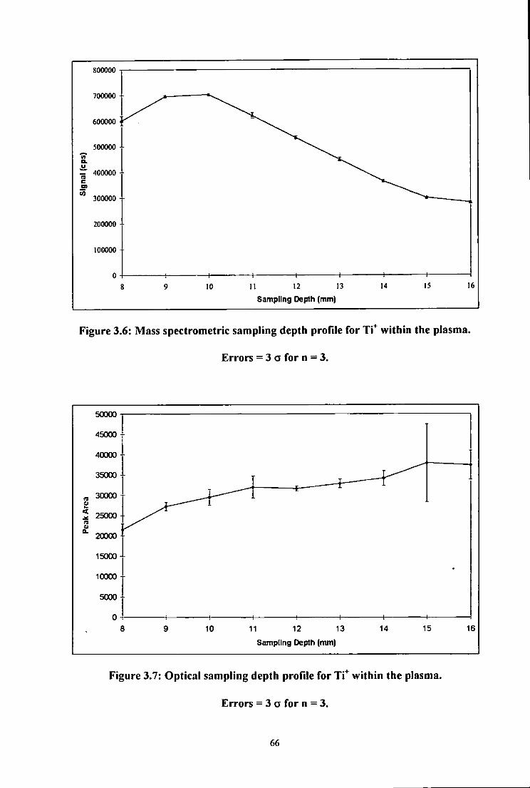
800000

700000

600000

500000

I ~ 400000 c V)

300000

200000

100000 4

10 M 12 13 Sampling Depth (mm)

14 IS 16

Figure 3.6: Mass spectrometric sampling depth profi le f o r T i ^ wi th in the plasma.

Errors = 3 a fo r n = 3.

40000 +

35000 +

30000

20000 -f

15000 +

10000 +

10 11 12 13

Sampling Depth (nun)

16

Figure 3.7: Optical sampling depth profi le fo r T i ^ w i t h i n the plasma.


66

These results show that the mass spectrometric signal for Ti* increased to a

maximum at a sampling depth o f 10 mm and then decreased as the sampling depth was

increased further, while the optical signal for T i " increased as the sampling depth was

increased, and levelled o f f at a sampling depth o f 16 mm.

This behaviour can be explained with reference to the two main zones in the ICP,

the initial radiation zone (IRZ) and the normal analytical zone (NAZ) . In ICP - AES the

N A Z is generally associated with the position at which the most intense ion line emission

is observed, while the 1R2 is where the most intense neutral atom line emission is

observed*^ ' ** . In ICP - MS the optimum observation zone is somewhere between the

IRZ and NAZ^^^, which is at a sampling depth o f approximately 5 - 1 5 mm ** . At small

sampling depths, corresponding to the IRZ, analytes introduced into the plasma have a

short residence time in the plasma. This short residence time in the plasma leads to

reduced ionisation o f the analyte species. As the sampling depth is increased the

residence time o f analytes in the. plasma increases, and so the analytes are present in the

plasma long enough for efficient ionisation to occur^^^. Therefore, as the sampling depth

is increased from the IRZ to the N A Z , the analyte signal intensity increases, as the

analyte is being more effectively ionised^°'*•^**^ However, at greater sampling depths the

plasma gas becomes cooler and so the ion population is lower, as the analyte is no longer

being effectively ionised at the lower temperatures and hence the analyte signal

decreases*^ . Therefore a zone o f maximum intensity is exhibited". This zone o f

maximum intensity was observed for the mass spectrometric signal, while the optical

signal had possibly just reached a maximum at a sampling depth o f 16 mm.

Previous studies on the effect o f sampling depth on metal analyte species include

Mg^ 139^ ,3M39^ ,39^ g ^ . 138,139,144^ pj^ . 138.139^ g ^ . 138^ 138^ 144

species were studied over different sampling depth ranges. However, the majority o f

species reached a maximum signal intensity at sampling depths between 5 and 10'mm,

67

and then decreased as the sampling depth was increased ftirther. The remainder o f the

species were studied at sampling depth ranges which started above 15 mm. These species

all reached a maximum signal intensity at the lowest sampling depth studied. The effect

o f sampling depth on the optical emission signals for Pb'^^, Cd'^***, Mg"^^**^-^" and Y*^^^

have also been studied. A l l o f the signals reached a maximum signal intensity at a

sampling depth around 10 mm.

Therefore, other studies show that the maximum analyte signal occurred at

sampling depths between 5 and 10 mm, which corresponds to the mass spectrometric

results o f this study, where the analyte signal reached a maximum at a sampling depth o f

10 mm. The optical results showed a maximum analyte signal at a larger sampling depth,

around 15 mm. However, this could be explained due to the system which is being

monitored optically. The previous optical studies have studied analyte species in an ICP -

AES, where the plasma is independent o f the detection optics. However, in this study

analyte species were studied optically in an ICP - MS, where the plasma is coupled

intimately to the extraction system which sits in the middle o f the plasma. Therefore, the

presence o f the extraction system within the plasma may aher the behaviour o f the

analyte species within the plasma.

Comparison o f the optical and mass spectrometric sampling depth profiles for Ti*

show no correlation between the two signals, whereas they would be expected to exhibit

the same trend as they are sampled fi*om the same region o f the plasma. However, while

the optical signal is sampled directly fi-om the plasma the mass spectrometric signal has

to travel through the mass spectrometer prior to detection. The influence o f the sampling

process, under high vacuum, is not known and this could explain the difference observed

in the optical and mass spectrometric data.

The mass spectrometric and optical sampling depth profiles o f TiO* and TiO

within the plasma are shown in Figures 3.8 and 3.9 respectively.

68

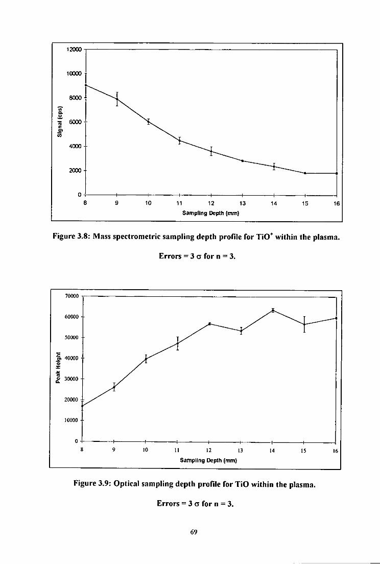
12000

10000

Sampling Depth (mm)

Figure 3.8: Mass spectrometric sampling depth profi le for T iO* wi th in the plasma.


70000

60000

50000

•g> 40000

20000

10000

P 30000 +

10 II 12 13

Sampling Depth (mm)

14 15 16

Figure 3.9: Optical sampling depth profi le fo r T i O wi th in the plasma.


69

These results show that the mass spectrometric signal for TiO"^ decreased as the

sampling depth was increased. At low sampling depths the analytes are being sampled

from the IRZ, where a short residence time in the plasma can lead to insufficient

dissociation o f any metal oxide species present in the plasma* "*. As the sampling depth is

increased the sampling region o f the ICP moves from the IRZ to the N A Z , resulting in

promotion o f MO"^ dissociation^ '***^. Molecular dissociation occurs progressively along

the axial channel o f the plasma^**^ because at larger sampling depths a long residence

time in the plasma results in effective dissociation o f the metal oxide. Therefore, a zone

o f maximum intensity is exhibited as the oxide is progressively formed and then

dissociated again. Therefore, at the sampling depths studied, which started at 8 mm, the

maximum signal intensity had probably already occurred lower down in the plasma, and

only the decrease in signal, as the sampling depth was increased from this position, was

observed.

Previous studies have investigated the effect o f sampling depth on various metal

oxide species, including CeO^ BaO"^ GdO' and TbO ' ^\ In all cases it was

found that either the metal oxide signal or the MO"" / ratio decreased as the sampling

depth was increased, as found in this study.

The optical sampling depth profile for TiO is shown in Figure 3.9. The optical

signal for TiO increased as the sampling depth was increased, until a sampling depth o f

12 mm, after which the signal remained fairly constant. This differed from the trend

observed for Y O by Furuta^°^ using ICP - AES. He found that the Y O emission was

localised low in the central channel o f the plasma, between sampling depths o f 0 and 10

mm, with a maximum occurring about 5 mm. However, in this study the analyte species

were being sampled from a plasma which is coupled intimately to the extraction system

which sits in the middle o f the plasma, and may alter the behaviour o f the analyte species

within the plasma.

70

Comparison o f the mass spectrometric and optical sampling depth profiles show

that the optical signal exhibited a diflferent trend from the mass spectrometric signal. The

optical signal for neutral TiO increased as the sampling depth was increased, while the

mass spectrometric signal for TiO* decreased as the sampling depth was increased. As

the sampling depth was increased the TiO* signal decreased as longer residence times in

the plasma resulted in more efficient dissociation o f the metal oxide ion. This was

reflected in the optical signal for neutral TiO, which increased as the sampling depth was

increased. Therefore, an increase in sampling depth resulted in a decrease o f the TiO*

signal and an increase in neutral TiO, as the TiO* was reduced to the neutral molecule.

Hence, simultaneous optical and mass spectrometric studies show that the TiO* ion was

not being dissociated in the plasma, but reduced to neutral TiO.

The optica! sampling depth profiles for TiO at diflferent positions o f the torchbox

are shown in Figure 3.10. The plots are arranged so that they are zeroed at the load coil

(sampling depth = 0 mm). Hence, the sampler cone was at sampling depths o f 8 mm (TB

- 0 ) , 11.5 mm (TB = 7) and 15 mm ( T B = 14).

These results show that at each position o f the torchbox (TB) the TiO signal

increased, reached a maximum, and then decreased again. This trend would be expected

for neutral metal oxides, which are most probably formed by collisional mechanisms*** .

At the load coil a low signal for neutral metal oxides would be expected, since there was

little time for these collisional processes to occur, and this signal would increase as the

sampling depth was increased, due to increased collisional formation o f MO. However,

molecular dissociation occurs progressively along the axial channel o f the plasma*** ,

which would lead to a decrease in the signal. Therefore, a maximum signal would occur

as the oxide was progressively formed and then dissociated again. In accordance to this

theory the plot for the maximum sampling depth profile (TB = 14) would exhibit this

trend, with the signal increasing, reaching a maximum and then decreasing again.

71

100000

80000

60000

• I B = 0 (8mm)

- ^ T B = 7 (11.5mm)

- * - T B = 14(15mm)

rz

CL

40000

20000

20 17.5 15 12.5 10 75 5 2 5 0 -2.5 Sampling Depth (mm)

-7.5

Figure 3.10: Comparison of optical sampling depth profiles for T iO wi th in the

plasma, at different sampling depth positions. Frrors = 3 a for n = 3.

However, the plots for ihc minimum (TB = 0) and the intermediate ( I B = 1) sampling

depth profiles had shorter measurable profiles, so it would be expected that the signal

was prematurely cut o f f by the tip o f the sampler cone, rather than decreasing naturally.

I his can be seen in Figure 3.10 where the signal for TB = 14 decreased gradually as the

tip o f the sampler cone was approached. The signal for TB = 7 decreased more sharply

as the tip o f the sampler cone was approached, although there was some indication that

the signal was beginning to decrease naturally, l l i e signal for T B = 0 decreased very

sharply as the tip o f the sampler cone was approached. Therefore, these results show that

with short sampling depth profiles the signal is greatly affected by the sampler cone,

which prematurely cut o f f the signal. However, with greater sampling depth profiles the

sampler cone was less significant as the signal began to decrease naturally.

72

3.3.2 Interface Studies (EfTect of Power)

A typical optical spectrum for (0 - 0) band emission from OH, showing the Qi

branches is shown in Figure 3.11. The optical power profile, within the interface, for the

Qi* branch, at 307.844 nm, of the (0 - 0) band emission from OH is shown in Figure

3.12.

309.5 308.5 Wavelength (nm)

Figure 3.11: Typical optical spectrum of OH (0 - 0) band emission showing Qi

branches.

These results show that the optical signal for OH in the interface remained fairly

constant as the power of the plasma was altered, although the signals obtained were not

very reproducible, with large RSDs at all powers studied. However, the sensitivity of the

fibre optic through the interface was less than half that through the fibre optic normally.

This can be seen in Figure 3.13, where a mercury lamp was used to obtain the mercury

line at 546.07 nm, which was used as a reference line throughout the optical studies.

73

2 0.8

5 0.6

O 0.4

Power (W)

Figure 3.12: EfTect of power on the signal for theQi' branch of the OH (0-0) band

emission at 307.844 nm within the interface. Errors = 3 a for n = 3.

70

60

3

^ AO <9

CO 20

10

Fibre Optic + Interface

Fibre Optic

545.5 545.6 545.7 545.8 545.9 546 546.1 Wavelength (nm)

546.2 546.3 546.4 546.5

Figure 3.13: Comparison of the optical signal for the Hg reference line (546.07 nm)

through the interface and without the interface.

74

This reduction in signal when monitoring the interface is illustrated in Figure 3.12, where

the signal obtained was very low, with poor reproducibility. These low signals and poor

RSDs meant that it was not possible to determine a meaningful trend in OH signal with

increasing power.

J. J. 2.1 OH Rotational Temperature

The OH optical emission data was used to calculate the rotational temperature,

from the slope of the graph log (I A. / A) against E , which is given by - 0.625 / T, where I

is the signal intensity, X is the wavelength, A is the transition probability, E is the energy

and T is the temperature, using the assignment, wavelength, energies and transition

probability data given in Table 3.4. An example plot is shown in Figure 3.14. This graph

was plotted for every power studied, in order to obtain a power profile of the OH

rotational temperature within the interface.

Table 3.4: Assignment, wavelengths, energies and transition probabilities for the

Q, branches of the OH (0 - 0) band^.

K X (nm) E (cm *) A (10** s *)

1 307.844 32,475 0.0

2 307.995 32,543 17.0

4 308.328 32,779 33.7

5 308.520 32,948 42.2

6 308.734 33,150 50.6

8 309.239 33,652 67.5

9 309.534 33,952 75.8

75

<

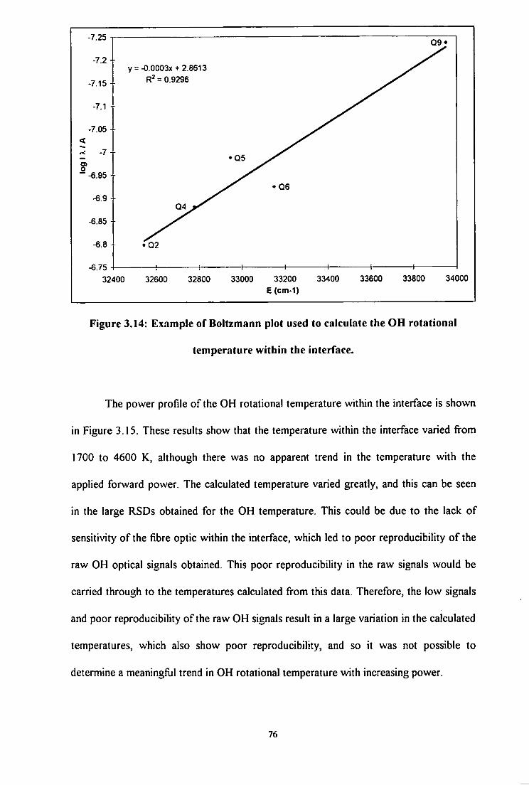
•7.25

-7.2

-7.15

-7.1

-7.05

-7

-6.95

-6.9

-6.85

-6.8

-6.75

Q9»

y = -0.0003x +2.8613 = 0.9296

•Q5

•Q6

Q4 > ^

• Q2

1 1 1 1 1 — t i

32400 32600 32800 33000 33200 33400 E (cm-l)

33600 33800 34000

Figure 3.14: Example of Boltzmann plot used to calculate the OH rotational

temperature within the interface.

The power profile of the OH rotational temperature within the interface is shown

in Figure 3.15. These results show that the temperature within the interface varied from

1700 to 4600 K, although there was no apparent trend in the temperature with the

applied forward power. The calculated temperature varied greatly, and this can be seen

in the large RSDs obtained for the OH temperature. This could be due to the lack of

sensitivity of the fibre optic within the interface, which led to poor reproducibility of the

raw OH optical signals obtained. This poor reproducibility in the raw signals would be

carried through to the temperatures calculated from this data. Therefore, the low signals

and poor reproducibility of the raw OH signals result in a large variation in the calculated

temperatures, which also show poor reproducibility, and so it was not possible to

determine a meaningful trend in OH rotational temperature with increasing power.

76

7000

6000

5000

o 4000 -a 2 V a. E 3000-o

j -

2000 -

1000

500 700 —,— 1100

1300 1500 1700 Power (W)

Figure 3.15: Effect of power on the OH rotational temperature within the interface

region of the ICP. Errors = 3 o for n = 3.

3.4 CONCLUSIONS

There was no correlation between the simultaneous optical and mass

spectrometric signals for T i \ although there was a definite correlation between the

optical signal of TiO and the mass spectrometric signal for TiO^ with the TiO signal

increasing as the TiO" signal decreased. Therefore, while mass spectrometric studies

would indicate that the dissociation of TiO* was enhanced with increasing sampling

depth, the simultaneous optical studies indicate that the TiO" was being reduced to

neutral TiO, rather than dissociated Ti* and O, due to the increase in the optical TiO

signal with increasing sampling depth. Therefore, the simultaneous optical and mass

spectrometric studies may provide an insight into the formation mechanisms occurring

within the plasma, which would not be possible with only mass spectrometric studies.

77

Both the Ti' and TiO signals monitored optically exhibited trends different to

previous studies performed with ICP - AES. This suggests that the extraction system,

which sits in the middle of the plasma in ICP - MS, may alter the detected signal of the

analyte species, when compared to optical measurements which are independent of the

mass detection system.

In the interface region of the ICP - MS the optical signals were very low v«th

poor reproducibility, which affected the OH rotational temperatures calculated from

them. This could be due to the reduced signal through the interface, which was half the

intensity of the signal not through the interface. However, in general it was very difficult

to detect any signal in the interface region of the ICP - MS, with the OH signal being the

only signal which could be determined within the interface.

Due to problems with the monochromator it was necessary to change the

operating software, and following this it was difficult to obtain signals in the plasma as

well as the interface, and so it proved very difficult to obtain signals which would be

sensitive enough to perform temperature or electron number density calculations. In

addition, the species of most interest to study optically in the plasma and interface, i.e.

the argon polyatomic ion interferences, suffered from a lack of available reference

wavelength data and so could not be measured optically. Therefore, although

simultaneous optical and mass spectrometric studies had the potential to provide

information on possible formation mechanisms and sites of formation, it was not possible

to study the analytes of interest with the equipment available.

78

CHAPTER 4

Critical Comparison Of Temperature Determination

Methods By ICP - MS

79

4 C R I T I C A L COMPARISON OF T E M P E R A T U R E

DETERMINATION METHODS BY ICP - MS

4.1 INTRODUCTION

A single temperature for the ICP cannot be determined explicitly because local

thermodynamic equilibrium (LTE) does not prevail in the plasma ****' . If the plasma is in

a state of L T E then Twin = Te = T„c = Tjon. However, this has been found to not be the

case for an argon atmospheric pressure ICP **, and the determined temperatures give

different values by the definition of the temperature. In general the temperature within

the ICP is decreasing in the order of electron temperature (Te), ionisation temperature

(Tion), excitation temperature (T„c) and rotational temperature (Trot) **"*.

The majority of techniques used to determine the temperature within the plasma

involve optical measurements, although it is also possible to calculate the temperature of

the plasma using mass spectrometric (jata*'* ' ** ' *'''"" *'', and both ionisation temperature,

(T,on) '** * and dissociation temperature, (Tdiss) '"" ^ '" * ''* have been calculated using

mass spectrometric means. The ion sampling process in ICP - MS is inherently radially

resolved, so there is no need to perform an Abel inversion, which is used in optical

emission experiments to construct radial emission profiles from line - of - sight intensity

measurements, thereby introducing substantial imprecision in the measured emission

profiles. Thus, mass spectrometric methods would be expected to produce more reliable

Tion values, provided that the relative ion abundances measured by the mass spectrometer

reflect the relative population of ions in the plasma **.

80

4.1.1 lonisation Temperature

The ionisation temperature can be calculated using the Saha equation **

(Equation 4.1)

log Kjon (M) = 1.5 log Tion - 5040 (IEm) / Ti^ + log (Zm^ / Zm) + 15.684 (4.1)

where Z = the partition function

IE = the ionisation energy

Tion = ionisation temperature

Kion = equilibrium constant.

If the relative abundances of the ions, atoms and electrons are known the equilibrium

constant can be calculated (Equation 4.2) and used to solve for Tion in the Saha equation.

M <-> + e Kien (M) = n.M n^ / nM (4.2)

where nM - = abundance of metal ion

n - = abundance of electrons

n\i = abundance of metal atom.

It is usual to calculate the temperature from the ratio of singly charged ions of

different elements which are similar in mass, thereby reducing the influence of mass bias

in the results. This involves the determination of the relative numbers of singly charged

ions formed from two elements (Mi and M2) of different ionisation energies * . The same

Tion is assumed for the reactions:

81

M, <->Mi' + e Ki (4.3)

Mz <^ M2' + e" K2 (4.4)

where K = equilibrium constant.

Subtracting the logarithmic forms of the Saha equation for K2 from that for Ki leads to

the relationship

log ( K , / K2) = [5040 (IE2 - IE,) / Tion] + log (2m,+ / Zm.) - log (Zm,. / Znu) (4.5)

The ratio of equilibrium constants in Equation 4.5 may be evaluated as follows

log (K, / K2) = log [(nMi+ / nM.+) (nM. / nM,)] (4.6)

nM-(l - o c ) C (4,7)

-(n,-/(nc- + K ) ) C (4.8)

log ( K , / K2) = log [(nM,. / hnu O (ne- + K i / n.- + K2) (C2 / C , ) ] (4.9)

where oc = the degree of ionisation

C = the solution concentration of the indicated element.

82

The ionisation temperature is taken to be that value which results in equivalence of

Equation 4.9 using n - values taken from the literature ' . This method has been used to

measure the ionisation temperature of the plasma by comparing the ratio of Cd* / T

SbVln^^^andAsVGa^^".

2-K3I3 These calculations can be extended to include doubly charged ions (M~*)

M" <-> M " + e' K'ioD (M) = nM2+ n - / nM+ (4.10)

log K'ion (M) = 1.5 log Tion - 5040 (IE') / Tion + log (Zm2+ / Zm+) + 15.684 (4.11)

where IE' = the second ionisaiion energy of the element M

Zm2+ = the electronic partition function of M^*.

2.1.2 Dissociation Temperature

There are several different methods which can be used to determine the

dissociation temperature within the plasma, all based on the dissociation of a diatomic

molecular ion ( X Y ^

XY" <^ X" + Y Kd ( X T ) = nv nx+ / nxv ^ (4.12)

where the equilibrium constant IQ is defined as ^

Kd = (Zx+ Z y / ZxY+) ((271 k T) / h') ((Mx+ My) / Mxy+)"' (hcB/k (1 - exp -(hc<o/kT)) /

T) exp(-Do/kT) (4.13)

83

where M = the species mass

Do = the dissociation energy

k = the Boltzmann constant

T = the plasma temperature

Z = the electronic partition function

B = the rotational constant

© = the vibrational constant.

The majority of these methods use the dissociation of metal oxides''* *"* ' *'' to

calculate the temperature, although other diatomic molecules, such as ArO" ^ ^ have also

been studied. This method could be used to obtain a dissociation temperature from most

diatomic molecules, as long as all the necessary fundamental data exists. A table of

existing fundamental data is given in Appendix

2.2 EXPERKMENTAL


Ion Path, Road Three, Winsford, Cheshire, UK), as described in Section 2.1.2. Both

ArX^ and MO"*" interferences were studied at the m / z shown in Table 4.1.

A radial profile of the plasma using standard conditions, at 1350 W, was obtained

by moving the torchbox from right to left across the tip of the sampler cone at 0.25 mm

intervals, at a sampling depth of 16 mm. A solution containing 10 ng ml * MASSCAL

(Be, Mg, Co, In, Pb and U) and 100 ng ml'* Al, Ba, La, Mn, Ti, Y and Zr (in order to

obtain MO^ signals) was aspirated into the plasma. At each position of the radial profile

the ion lens and torchbox position in the other two axes were adjusted to obtain a

maximum signal for "^In*.

84

Table 4.1: Isotopes studied during radial profile experiment

Species Mass Abundance Species Mass Abundance

Al' 27 100 89 100

Ar' 38 0.1 Zr^ 96 2.8

ArH" 39 0.1* Y O ' 105 99.8*

AIO^ 43 99.8* ZrO^ 106 51.3*

Ti^ 49 5.5 In' 115 95.8

Mn^ 55 100 Ba' 132 0.1

ArO' 56 99.4* La' 138 0.1

TiO' 64 73.6* BaO' 154 71.6*

Ba^' 66 0.1 LaO' 155 99.7*

MnO^ 71 99.8*

* The abundances for the molecular species were calculated by combining the

abundances of the two constituent elements. Molecular abundances were obtained by

multiplying abundances of constituent elements and then dividing by 100.

4.3 RESULTS AND DISCUSSION

4.3.1 Radial Profile of ArX^ and MO* Species

Indium was introduced to act as an internal reference to determine the centre of

the plasma. Because the indium solution was aspirated into the plasma the majority

should pass through the centre of the central channel, with little signal being observed

beyond the central channel of the plasma. The results for *'^In', shown in Figure 4.1,

indicate that as the torchbox was moved from right to left across the tip of the sampler

cone the signal increased, reaching a maximum and then decreased again.

85

350000

300000 +

250000

« 200000

c § 150000

100000

50000

-0.5 0 0.5

Radial Position (mm)

1.5

Figure 4.1: Radial profile for "^In*. Errors = 3 a for n = 3

This has been observed for the optical emission of Y"" and Mg^ where the

maximum signal occurs on - axis (i.e. the centre of the plasma) with little signal being

observed beyond 3 mm either side of the central axis. Therefore, the position where the

maximum In^ signal was observed in the radial profile of the plasma was taken to be the

centre of the plasma. This trend can also be seen for other species which were introduced

into the plasma, as shown in Figures 4.2 and 4.3 for '' Ba' and * Ba ^ respectively.

For these species the signal also exhibited a maximum signal along the central

axis, as defined by the In" signal, and decreased as the distance from this central axis was

increased, with little signal being observed at either edge of the profile. This was also the

case for interferences such as metal oxides because, although oxygen is present

throughout the plasma, the metals were only introduced through the central channel. This

can be seen in Figure 4.4 where the radial profile of all of the seven metal oxides studied,

as given in Table 4.1, are compared.

86

4500

4000 -}-

3500

3000 i

fi- 2500 +

|> 2000

1500

1000 - f

500

0 -2 -1.5 -0.5 0


0.5 1.5

Figure 4.2: Radial profile for Ba^ Errors = 3 a for n = 3.

45000

40000

35000

30000 +

S. 25000

m 20000

15000

10000

5000 -

0 --0.5 0

Radlat Position (mm)

0.5 1.5

Figure 4.3: Radial profile for Ba"*. Errors = 3 a for n = 3.

87

2000000

1800000

1600000

1400000

- 1200000 a

o ^ 1000000 c at

« 800000

600000

400000

200000

0

LaO (Do = 8 88eV)

ZKXDo = 7 76eV)

YCK (Do = 7 24eV)

T i O (Do = 6 93eV)

BaO (Do = 4 09eV)

MnCH (Do = 2 75eV)

AJO(Do= 1 71eV)

1 5 -1 -05 0 Radial Position (mm)

05

Figure 4.4: Comparison of the radial profiles for MO . Signals normalised to 100%

abundance (Signals divided by molecular abundance then multiplied by 100).

Molecular abundances of metal oxides are given in Table 4.1. Do values given are

for M O \ Errors = 3 a for n = 3.

Figure 4.4 shows that all of the metal oxides studied exhibited the same trend,

with a maximum signal along the central axis of the plasma, and the signal decreasing as

the distance from the central axis was increased, with little signal being observed at either

edge of the profile. However, the maximum intensity reached varied considerably

between each metal oxide species. It can be seen that the intensity of the metal oxide

signal varied according to its dissociation energy. Species with a high dissociation energy

require large amounts of energy to break the metal oxide bond, so were present in the

plasma in large quantities, and hence a large signal was observed. Conversely, species

with low dissociation energies require little energy to break the metal oxide bond, were

present in the plasma in very small quantities because they have dissociated to a greater

sx

extent, so relatively little signal was observed. This can be seen in Figure 4.4 where

LaO\ with a high dissociation energy of 8.88 eV, gave rise to a very large signal and

AlO*, with a low dissociation energy of 1.71 eV, produced virtually no signal.

Other interference ions, such as ArO^, showed a broadly similar trend to the

metals and metal oxides, as shown in Figure 4.5.

3500000

3000000

2500000

^ 2000000 c

1500000

1000000

500000 1.5 -1 -0.5 0 0.5


1.5

Figure 4.5: Radial profile for ArO*. Errors = 3 o f e r n = 3.

Figure 4.5 shows that the signal for ArO" still reached a maximum signal

intensity, although the maximum was spread over a wider distance than for the metal

analyte species. At the edges of the radial profile the signal intensity did decrease but not

as rapidly as for the other species, and there was still a relatively large signal at the edges

of the radial profile, whereas the signal intensities for the metal oxides were minimal at

these positions. These results suggest that, although there is more oxygen entering the

plasma through the central channel with the aspiration of the analyte solution in 2 %

89

HNOs, there were also significant amounts of both argon and oxygen throughout the rest

of the plasma, indicating that there were significant levels of ArO" being formed in parts

of the plasma beyond the central channel.

4.3.2 Temperature Determination

The generalised methods for determining the temperature in the plasma,

described in Section 3.1, have been used by various workers''* ' '* '"*** '*' ''*. However,

several problems exist with the application of these methods and the interpretation of

their results, as discussed in the following sections.

4.3,2,1 Method A

This method was first proposed by Douglas and French **, and applied by

Longerich^***. The assumption is made that MO" / N4 oc e^'^\ and that the temperature

can be determined fi-om the energy of formation of the monopositive monoxide ion fi-om

the corresponding monopositive metal ion (M" ) ***.

The equilibrium of the metal oxide monopositive ion with the monopositive metal ion

and neutral oxygen is given as

MO" -> + O dissociation energy = Do (4.14)

Do = - RT In ([MO'] / [M' ] ) (4.15)

This equation can be rearranged to

log ([MO^] / [M^]) = Do/ [RT X In (10)] + constant (4.16)

90

where [MO*]/[>f ] = the measured ratio of the metal oxide and metal ion signals

Do = the dissociation energy of the metal oxide

R = the universal gas constant

T = the temperature.

A plot of y = log ( [ M 0 1 / [M1) versus x = Do gives a straight line where

s l o p e = l / [ l n ( 1 0 ) x R T ] ( 4 . 1 7 )

Rearrangement of this equation gives

T = l / [ l n ( l O ) x R x s l o p e ] (4.18)

The constant (intercept) is a function of the fugacity of oxygen and is constant for a set

of elements determined at a given set of operating conditions. This graph was plotted for

every point of the radial signal profile, in order to obtain a radial profile of the

temperature. An example plot is shown in Figure 4.6.

0

-0.5

-1

-1.5

-2

-2.5

-3

-3.5

-4

-4.5

y = 9E-06x-7.0157 R' = 0.9836

Slopes 1/pn(10)xRTl

300000 350000 400000 450000 500000 550000 600000 650000 700000 750000 800000

Dissociation Energy (J/mol)

Figure 4.6: Example of plot used to calculate the temperature using Method A.

91

This was initially plotted with the dissociation energy data for the neutral metal oxides,

for a direct comparison with previous calculations which have erroneously used the MO,

rather than the MO^, dissociation energies due to the limited MO* data. However, the

MO" dissociation energy data did exist for most of the metal oxides used in this study

and it was possible to calculate the others using Equation 4.19^^^

Do (MO") = Do (MO) - lE(MO) + IE(M) (4.19)

These values were then used to calculate the temperature using the Do ( M O ^

data, in graphs similar to Figure 4.6. These graphs were plotted for every point of the

radial signal profile, in order to obtain a radial profile of the temperature using the Do

(MO*) data. The differences between Do (MO*) and Do (MO) are shown in Table 4.2.

Table 4,2: Comparison of Dp (MO) and Do {MO^ values

Metal Do(MO)/eV Do (MO") / eV

Al 5.27 1.71

Ba 5.79 4.09*

La 8.23 8.88

Mn 3.71 2.95

T i 6.87 6.93

Y 7.39 7.25

Zr 7.85 7.76

* = value calculated using Equation 4.19.

The radial temperature profiles determined using this method are shown in Figure 4.7.

92

18000

160CX)

14000

12000 T

10000

I 8000 o

6000

4000

2000 -

0

Do (MO) » •Do(M04-)

H — •1.5 -0.5 0

Radial Position (mm) 0.5 1.5

Figure 4.7: Comparison of the radial profiles for the temperature calculated using

Method A, with data for Do (MO) and Do (MO"^. Errors = 3 CT f e r n = 3.

The temperature determined using the MO dissociation energies ranged fi'om 6200 K at

the central axis of plasma to 14,500 K at the edges of the radial profile. The temperature

calculated using the MO^ dissociation energies v/as slightly higher than that for the MO

data, ranging fi-om 7400 K at the central axis of the plasma to 16,000 K at the edges o f

the radial profile. The temperatures using both sets of dissociation energies were much

lower than other temperatures reported using this method, 21,000 K^^^ and 12,500 K '**,

although Longerich'^^ also reported a lower temperature of 10,100 K using this method.

The temperatures calculated using this method, except at the very edges of the radial

profiles, were within the range expected in the plasma (5000 - 10,000 K)^^^.

The radial profiles of the temperature exhibited the opposite trend to that shown

by the raw data, i.e. the temperature was lowest at the central axis and increased as the

distance ft-om this central axis was increased. This trend was also observed by Komblum

and De Galan^" for the excitation temperatures of Ar, Ca and Mg and the OH rotational

93

temperature. This would be expected because the aspiration of solution through the

central channel cools this region of the plasma relative to the outer regions. Therefore, it

would be expected that the central channel of the plasma was the coolest part of the

plasma, and that the temperature increased as the distance fi-om the central channel was

increased.

The raw data plots used to calculate the temperature, e.g. Figure 4.6, indicate the

magnitude of inherent errors in these temperature calculations. Towards the edges of the

radial profile, where the raw signals were low, poor values were obtained, e.g. 0.87.

However, near the central axis, where the raw signals were high, the points were much

less scattered about the slope of the graph, as demonstrated by R^ values of 0.98 and

higher.

Previous studies using this method have used the dissociation energies of the

neutral metal oxides to calculate the dissociation temperature, due to the lack of available

data for the MO' species. The MO' data for the majority of the metal oxides used in this

study were available, but in general the available M O ' data is still limited, with the data

for most species not available, and that which is available is not easily obtainable. The

use of the M O ' dissociation energies produced an increase in the calculated temperature,

but which was still within the range expected in the plasma.

4.3.Z2 Method B

This method, developed by Kubota et al. '*", is also based on the relationship

between the measured metal oxide ion to metal ion signal ratio (SMO+ / SM+) and the

oxide bond strength (Do). However, they devised an expression which uses the

dissociation energies of the neutral metal oxides (Equation 4.20), and hence it is not

necessary to know the dissociation energies of the metal oxide ions.

94

nMo / HM = ZMO / ( -2K M M MQ kT / h MMO)^'^ Z M ZO X no exp (Do / kT) (4.20)

where n = the number density

M = the atomic or molecular weight

Z = the partition function

subscripts M , O and MO indicate a metal element, oxygen and a monoxide.

For the ionisation equilibria

M ^ M " + e (4.21)

and

MO o MO^ + e (4.22)

the equilibrium constants are

Ki =nM4-ne--/nM (4.23)

and

= nMo nc-1 n.Mo (4.24)

The elimination of nc- from equations 4.23 and 4.24 gives

nMo+ / nM+ = K 2 HMO / Ki nM (4.25)

Substituting equation 4.20 for equation 4.25 and rearranging gives

HMO^ ZO ( M M Mo / MMO)^'^ / nM+ ZMO = K 2 no exp (Do / kT) / K, (-27ikT / hY'^ (4.26)

95

Assuming that the signal ratio SMO - / SM+ equals nMo - / nM -

log [ SMO- ZM ZO ( M M MQ / MMO)"'/SM+ ZMO] = A + log ( K 2 / K,) + 5040 Do/ T ( 4 . 2 7 )

where A = log [no / ( -27 ikT /hV ' ]

Therefore, assuming K 2 / Ki is constant, the left hand side of Equation 4.27, i.e. the

logarithmic term in which the partition functions, atomic weights and molecular weights

are taken into consideration, should have a linear relationship with Do. This was plotted

for every point of the radial signal profile, in order to obtain a radial profile of the

temperature. An example plot is shown in Figure 4.8.

-72.5

(0

I g -73.5

If-74.5 + S N

i l -75+ N ^

E -75.5 N

-76

§» -76.5

-77

y = 0.e003x-79.254 R = 0.9671

slope = 5040 / T

Mn

Al

5 6 Dissociation Energy (eV)

Figure 4.8: Example of plot used to calculate the temperature using Method B

96

The need to know the dissociation energies of the metal oxide ions has been

overcome by this method, but other assumptions have been introduced. The calculation

of the temperature using Equation 4.27 assumes that the ratio of K 2 / K i is constant for

all the different metals and their oxide ions studied. This method introduces the partition

functions into the calculation, which are, by definition, a temperature dependent term.

Therefore, an assumption about the temperature of the plasma has to be made in order to

calculate the partition functions, which may affect the resultant temperature calculated

using that data.

The radial temperature profile calculated using Method B is shown in Figure 4.9.

The temperature determined ranged ft-om 6200 K at the central axis of plasma to 15,000

K at the edges of the radial profile. These temperature values were almost identical to

those calculated for Method A using the MO dissociation data. The temperature profile

also followed the same trend as shown for Method A, in that the temperature was

coolest at the central axis of the plasma and increased as the distance fi^om this central

axis was increased.

16000

14000 4

12000

g 10000

I ^ 8000

6000

4000 +

2000

0 -1.5 -0.5 0 Radial Position (mm)

0.5 1.5

Figure 4.9: Radial profile for the temperature calculated using Method B. Errors

3 a for n = 3.

97

These temperatures determined using Method B corresponded to other

temperatures calculated using this method (6650 K)'*" and lay within the expected values

for the plasma (5000 - 10,000 K)"^.

As with Method A the raw plots used to calculate the temperature (e.g. Figure

4.8), were variable, with poor values obtained for the edges of the radial profile (e.g.

« 0.86). However, near the central axis the points were much less scattered about the

slope of the graph, with R^ values of 0.97.

4.3,2.3 Method C

This method has been suggested by Houk^^^, and is based on the theory that the

dissociation of a diatomic molecule at a gas kinetic temperature (Tgas) is governed by an

equation similar to the Saha equation ** . The main reaction for the dissociation of an

oxide ion MO* is

MO^ M" + 0 (MO") = no n.M^ / nMo (4.28)

where the equilibrium constant IQ is defined as ^

K, = ((271 M M MO) / (h ' MMO) kT) ' ' ' (ZM ZO / ZMO) exp (-Do / kT) (4.29)

where M = the species mass

Do = the dissociation energy (eV)

k = the Boltzmann constant

T = the plasma temperature

Z = the partition fijnction.

98

Equation 4.29 can be rearranged to include the spectroscopic constants of MO"^ rather

than the partition fijnction, which is difficult to evaluate, as given in Equation 4.30.

log Kd = log Z M Z O + 0.5 log T + log ( M O ^ " ^ c / F J _ 5Q4Q / T + C ( 4 . 3 0 )

where

C = 20.432 + 1.5 log ( M M + M O / M M O ) + log ( B / g) ( 4 . 3 1 )

where g = the statistical weight of the ground electronic state of M O *

CO = a vibrational constant (cm'*)

B = a rotational constant (cm"*)

M = the atomic or molecular weight.

Combination of Equations. 4.30 and 4.31 gives 142,249

log ( M O " ) = 0.5 log Tgas - 5040 Do / Tg s + 1.5 log (MN,. M Q / MMO) + log (ZM^ ZQ)

+ log ( I - 10 + log (B / g) + 20.432 (4.32)

Temperature measurements using this method may be inaccurate due to the use o f

partition fianction values, which are, by definition, temperature dependent. However, in

the case of ions and neutral atoms the electronic partition function can be calculated

using equation 4.33, with the appropriate constants **.

B(T) = a + b (T/10^) + c (T/IO') ' + d (T/10^)' + e (T/IO')' + f (T/IO')' (4.33)

99

For the calculations undertaken here the value for the partition fijnction (Zx) did not rely

upon a single temperature value, because a spreadsheet was set up so that the value for

the partition ftinction changed as the temperature value was altered.

The resuhs obtained fi-om Section 4.3.1 were used to calculate an experimental value for

Ki ( M O ' ) using Equation 4.34.

Kd ( M O ' ) = no nM+ / n.Mo (4.34)

This was calculated by measuring the signals for M ' and M O ' in order to obtain an nM+ /

nMo+ ratio. This was then multiplied by the theoretical value of oxygen atoms in the

plasma, calculated using Equation 4.35 '* .

no = Encb F No Troom / MH20 Q f plasma (4.35)

where £ n c b = nebuliser efficiency (= 2 %)

F = solution uptake rate (= 1.2 ml min * = 0.02 g s'*)

No = Avagadro's number

Mn2o = molecular weight of water (= 18 .015 g mol'*)

Q = gas flow rate (= 0.9 1 min'* = 15 cm^ s' )

Troom = room temperature (= 292 K)

Tpiasma = plasma temperature (= 5000 K).

This value, of 5.21 x lO'^ atom cm'^ is the contribution of 0 atoms fi-om the water

droplets. However, there is also a contribution of O atoms fi-om water vapour, calculated

using Equation 4.36^^^

100

no(vap) = P / R Tspniy X {Jspr^y I TpUsma) (4.36)

where P = vapour pressure of water (= 1498 Pa)

R = gas constant (= 8.31451 J K * mol"*)

Tfipray = temperature of spray chamber (= 289 K)

Tpiaana = plasma temperature (= 5000 K).

This value, of 2.17 x lO'^ atom cm^ is the contribution of O atoms fi-om the water

vapour. The value for the amount of 0 atoms in the plasma is obtained by combining the

contributions fi-om water droplets and water vapour, resulting in a value of 7.38 x 10*

atom cm'^

This experimental value of Kd (MO"^ was then compared to the theoretical

(MO*) value, calculated using Equation 4.28. Using a spreadsheet, the value for the

temperature was adjusted until the theoretical Ka value was the same as the experimental

Kd value. This temperature was then assumed to be the equilibrium dissociation

temperature for the MO^ species.

Unfortunately, the spectroscopic constants for most of the MO" species do not

exist, therefore, the spectroscopic constants for the neutral metal oxides had to be used

instead. A table of the spectroscopic constants which are available is given in Appendix

| 3 i5-33i p i Q ^ g v e r , the spectroscopic constants for AlO* were available, and a comparison

of these with the spectroscopic constants for neutral AlO is shown in Table 4.3. In order

for a complete comparison of AlO and AlO" the dissociation energy of AIO" was used.

The radial profiles of the temperatures calculated ft*om the dissociation of each of

the seven metal oxides studied, as given in Table 4.1, are shown in Figure 4.10.

iOl

Table 4.3: Comparison of spectroscopic constants for AlO and AlO

Spectroscopic Constant AlO AlO*

(0 / cm ' 979.23 710

B / c m ' 0.64136 0.5066

g 2 6

7500

7000

6500

6000

f 5500 3

5 5000

I 4500

4000

3500

3000

2500 -15 -1

^ L a O ( O o = = 8 23eV) -ii-ZrO(Do = 786eV)

• YO(Do = 7 39eV) - ^ T O ( D o = 687eV) • BaO(Do = 5 79eV)

^ AIO(Do = 527eV) MnO(Do = 3.71eV)

-05 0 0.5


15

Figure 4.10: Comparison of the radial profiles for the temperatures calculated

using Method C, with Do values for MO. Errors = 3 a for n = 3.

The temperatures calculated for the dissociation of BaO, LaO, YO and ZrO

exhibited the same trend as for Methods A and B, in that the temperature was lowest at

the central axis of the plasma and increased as the distance from this central axis was

increased. The temperature calculated for the dissociation of AlO, MnO and TiO

exhibited the opposite trend, in that the temperature was greatest at the central axis of

the plasma and decreased as the distance from this central axis was increased.

102

The resuhs of Methods A and B, and the work of others^" all indicate that the

temperature should be lowest at the central axis of the plasma and that it increases as the

distance fi-om this central axis is increased. This was the case for four of the seven metal

oxides studied, i.e. BaO, LaO, YO and ZrO, and indicates that there may be a problem

with the temperature calculation for the other three metal oxides, i.e. AlO, MnO and

TiO. Inspection of the raw data for these species seems to suggest that this was the case.

The raw signal for MnO* was negligible and therefore this would lead to a large error in

the Mn* / MnO" ratio, which in turn would lead to a large error in the temperature

calculated fi'om this data. This was also the case for AlO*, although not to such an extent

as for MnO*. There was ample signal for TiO*, so this was not the reason for an unusual

trend in the temperature calculated for TiO*. However, a 10 ng ml * of MASSCAL was

aspirated along with the solution used to obtain the metal oxide signals. The MASSCAL

solution contained Be at m / z = 9, and so there was the possibility of this reacting with

Ar to form the interference ion ArBe*, which would interfere with the isotope of Ti*

monitored at m / z = 49. There was also the possibility of a minor isotope of NO2*,

formed fi-om the 2 % HNO3 solution, causing an interference at m / z = 49. Therefore,

these would lead to a deviation fi-om the correct Ti* / TiO* ratio, and hence an error in

the temperature calculated fi-om this ratio.

Despite the differences in the trends for the temperatures calculated fi'om the

different species, all of the temperatures calculated were within the range 4000 - 7000 K,

which is well within the range expected in the plasma ^ . The temperatures calculated

exhibited no correlation with the dissociation energy of the metal oxide species.

The temperatures calculated fi'om the data for the neutral metal oxide and the

metal oxide ion of AlO are compared in Figure 4.11.

103

7000

6000

5000

S 4000

E 3000 CI

2000

1000

-^AlO (Do = 5.27eV)

• ••AI0+ (Do = 1.71 eV)

-1.5 -0.5 0 Radial Position (mm)

0.5 1.5

Figure 4 . 1 1 : Comparison of the radial profiles for the temperature calculated using

Method C, with data for A I D and A I O ^ Errors = 3 a fern = 3.

The temperature calculated fi-om the data for the metal oxide ion was much lower

that that calculated fi'om the data for the neutral metal oxide. The temperature calculated

for AlO ranged ft*om 5400 to 6250 K, whereas the temperature calculated for AlO"

ranged ft-om 2000 to 2350 K. This is different to Method A where the temperature

calculated with the metal oxide ion data was higher than that calculated with the neutral

metal oxide data. This may be due to the fact that the dissociation energy of AIO* was

much lower than that for neutral AlO (1.71 eV as compared to 5.27 eV). AIO^, with a

lower dissociation energy than the neutral AlO, would require less energy to dissociate

the molecule, resulting in the dissociation equilibrium being reached at a lower

temperature, and so a lower temperature would be expected for the dissociation of AlO"^

compared to that for AlO. However, this lower temperature calculated for the

dissociation of AlO* (< 2500 K) was much lower than would be expected within the

plasma (5000- 10,000 K ) ' "

104

4.3.2.4 MethodD

This method has been utilised by Houk et al}^^ and is based on the ionisation of

an already ionised metal ion. A set of ionisation reactions can be written for the major

plasma constituents (Ar, H and 0) , the matrix elements (X) from the sample, and the

analyte elements (M)^'*^ e.g. for metal analyte

M <^ IvT + e Kion (M) = fiM^ ne- / n.M (4.37)

The ionisation constant can be calculated from the Saha equation "*

log Kion ( M ) = 1.5 log T i ^ - 5040 ( IEM) / Tjon + log ( Z ^ . / Z M ) + 15.684 (4.38)

where I E M = the first ionisation energy for the element M (eV)

Z = the partition function

Tion = the ionisation temperature (K).

These calculations can be extended to include doubly charged ions (M^^).

NT <^ M ' ' + e" K'ian (M) = nM2+ nc- / n^^ (4.39)

log K'iox, (M) = 1.5 log Tion - 5040 ( I E ' ) / Tion + log (ZM2. / Z M . ) + 15.684 (4.40)

where I E ' = the second ionisation energy of the element M

ZM2+ = the electronic partition function of M^^.

105

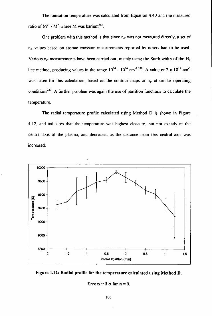
The ionisation temperature was calculated from Equation 4.40 and the measured

ratio of M^^ / where M was barium^

One problem with this method is that since nc- was not measured directly, a set of

n - values based on atomic emission measurements reported by others had to be used.

Various n^ measurements have been carried out, mainly using the Stark width of the Hp

line method, producing values in the range lO*'* - 10* cm'^"^. A value of 2 x 10* cm'

was taken for this calculation, based on the contour maps of nc- at similar operating

conditions'^'. A further problem was again the use of partition functions to calculate the

temperature.

The radial temperature profile calculated using Method D is shown in Figure

4.12, and indicates that the temperature was highest close to, but not exactly at the

central axis of the plasma, and decreased as the distance from this central axis was

increased.

10000

9800 4

_ 9600

I* 5 9400 u a

9200

9000 i

8800 •1.5 -0.5 0 0.5


1.5

Figure 4.12: Radial pronie for the temperature calculated using Method D.

Errors = 3 a for n = 3.

106

The temperature calculated using this method was higher than those calculated

using the previous methods, varying from 9300 K at the edges of the radial profile to

10,000 K around the central axis of the plasma. This higher ionisation temperature would

be expected because the plasma is not in thermal equilibrium, and values for the

ionisation temperature are typically higher than those for the dissociation and excitation

temperatures'^^

Other Tion determinations have also produced temperatures which are higher than

those determined for excitation and dissociation temperatures (5000 - 7000 K). Mass

spectrometric Tjon measurements have produced temperatures of 7600 - 8000 K using

Ba V Ba* and Sr V Sr ratios, and 7800 - 8400 K using the Cd^ / V ratio, for n - values of

2x10'^ cm" ^'^ The Cd" / T ratio has also resulted in ionisation temperatures of 6700 -

7400 K^*^ while the ratios of Sb^ / In" and As^ / Ga"" have resulted in ionisation

temperatures of 6850 K and 6450 K respectively^*'. Optical Tion measurements have

resulted in temperatures of 8100 K using Ca"^'"^ 7600 K using Ba"^ and 8000 K using

Mg""* as the thermometric species, at similar n - values (2 x lO'^ cm'^). However, the

power used for these studies, 1 kW^ '"* ^ and 530 W^^ , was much lower than used in this

experiment. A Tjon value of 7200 K for Mg was obtained at the same power as used for

this experiment (1350 W) '*'', although the observation height was very low (2 mm) and

the nc- value used was only 5 x lO'** cm'^. All of the optical Tion measurements were

calculated using the / M ratio.

The trend shown by the temperature, with the highest temperature being along

the central axis of the plasma, is different to that which would be expected, i.e. with the

central channel of the plasma being cooler than the outer areas due to cooling by the

solution being aspirated. This could be due to a very minor isotope of Ba " (m / z = 66 at

0.1 % abundance) being monitored, which would probably suffer from interference by a

minor isotope of TiO"" (m / z = 66 at 5.4 % abundance) which would also be present

107

since it was one of the species being studied. However, the isotopic ratio of TiO* was

known, and so the contribution of the signal at m / z = 66 which was due to TiO* was

calculated and corrected for.

4.3.15 Method E

A similar reaction to that described in Section 4.3.2.3, for the metal oxides using

Method C, can be written for the dissociation of other polyatomic ions, such as ArO" ^**'.

ArO^ <^ + AT Ki (ArO') = no ^ nAr / nAK)+ (4.41)

log (ArO') = 0.5 log • 5040 Do / Tgas + 1.5 log (MATMo- / MAro+) + log {Z^Zo^)

+ log( l - 10 +log ( B / g ) +20.432 (4.42)

The results obtained in Section 4.3.1 were used to obtain an Ar^ / ArO" ratio, which was

then divided by the degree of ionisation for argon, in order to obtain the value for Ar /

ArO^. This value was then multiplied by the theoretical value of oxygen atoms in the

plasma, calculated previously in Section 4.3.2.3. This value was then multiplied by the

degree of ionisation for oxygen in order to obtain the amount of O" (5.99 x lO''* atoms

cm'^) in the plasma. However, species such as ArO"" are thought to form in the interface

of the ICP - MS rather than in the plasma and so another Ka value was calculated using

the oxygen ions concentration assumed to be in the interface (1.97 x 10* atoms cm"^),

calculated using Equation 4.43^ '

nx (int) = 0.161 nx(plasma) ( D / x ) ' (4.43)

108

where nx(piasma) = the density of the species X in the plasma

X = the position downstream from the sampling orifice

D = the sampling diameter.

The experimental IQ (ArO^ value, calculated for both the plasma and interface was

compared to the theoretical (ArO^ value as described previously for Method C in

Section 4.3.2.3. Alternatively, K\ (ArO"^ can be calculated by measuring the / ArO"

ratio, which was then multiplied by the concentration of argon assumed to be in the

plasma (1.45 x 10 ^ atoms cm*'), calculated from the ideal gas law'", to obtain a IQ

(ArOO value for the plasma. The amount of Ar in the interface (4.76 x lO'^ atoms cm'')

was calculated using Equation 4.43 and used to obtain a (ArO*) value for the

interface. These experimental Kd (ArO^ values, calculated for both the plasma and

interface were then compared to the theoretical Kd (ArO"^) value as described previously.

The results are shown in Figure 4.13, and indicate that the temperature was

lowest at the central axis of the plasma, and increased as the distance from this central

axis was increased. This trend is the same as that which would be expected, with the

central channel of the plasma being cooler than the outer areas due to cooling by the

solution being aspirated.

The temperature calculated for the plasma using this method was much lower

than those calculated for the other methods, varying from 650 K at the central axis o f the

plasma to 2250 K at the edges of the radial profile studied. This is much lower than

would be expected in the plasma (5000 - 10,000 K), and this could be due to the low

dissociation energy of ArO*, which is only 0.43 eV. This is much lower than the metal

oxides, the lowest being MnO with a dissociation energy of 3.71 eV. However, AlO^

also has a dissociation energy much lower than the neutral metal oxides (1.71 eV), and

the temperatures calculated for this species were also much lower than those expected

109

within the plasma (< 2500 K). Therefore, the low temperature calculated for ArO* may

be due to its low dissociation energy, although the metal oxides showed no trend

between the temperature and the dissociation energy of the molecule.

3000

2500

_ 2000

I 1500

I 1000

500

Plasma Interface

— i —

-1.5 -0.5 0


0.5 1.5

Figure 4.13: Comparison of the radial proflles for the temperature calculated using

Method E, for equilibration in the plasma and interface. Errors = 3 a for n = 3.

Argon polyatomics, such as ArO", are thought to possibly be formed in the

interface rather than in the plasma''*^ and this may reflect the low temperature. The

temperature calculated for the interface was even lower than that calculated for the

plasma, ranging from 350 K at the central axis of the plasma to 600 K at the outer edges

of the radial profile studied.

These temperatures calculated for both the plasma and interface were much

lower than expected for the plasma. The temperature calculations are based on partial

local thermodynamic equilibrium (p - LTE) conditions within the plasma, and therefore

the low temperatures calculated using ArO* may indicate a deviation from LTE

110

conditions. LTE conditions are not thought to exist in the interface region of the ICP -

MS, suggesting that the ArO^ species is formed in the interface rather than the plasma.

The low temperatures calculated correspond to those thought to prevail in the interface

(< 3500 K) ' ' ' ^ also suggesting formation in the interface rather than the plasma.

4.4 CONCLUSIONS

4.4.1 Method A

The temperature calculated using Method A varied between 6150 and 14,500 K,

which was much lower than those previously reported for this method, which were as

high as 21,000 K **. These previously high temperatures were thought to be due to the

incorrect use of the neutral metal oxide dissociation energies. However, the combination

of metal oxides used in this study enabled the determination of the temperature using the

dissociation energies of the metal oxide ions, which were available for these species. The

temperature calculated using the Do (MO*) values were slightly higher than those for Do

(MO), varying between 7400 and 16,000 K. These values are higher than temperatures

reported by other workers using optical methods to determine the temperature (4000 -

7000 K), but apart from at the extreme edges of the radial profile, the calculated

temperatures lie within the range expected for the plasma (5000 - 10,000 K)"^.

The metal oxides species used in this study have Do (MO) values similar to their

Do (MO*) values, and this could explain the similar temperatures calculated using the two

sets of dissociation energies, whereas previous studies reported temperatures up to

21,000 K using the Do (MO) values. The metal oxide species used in these previous

studies were different to those used in this study and the Do (MO*) values were not

necessarily available for these species. I f the Do (MO) and Do (MO*) values for these

111

species are not similar, this might result in the extremely high temperatures calculated in

these studies using the Do (MO) values.

Therefore, the problem of extremely high calculated temperatures previously

associated with this method were overcome by using the correct Do (MO*) values.

However, this was only possible because the Do ( M O ^ values were obtainable for the

metal oxide species used in this study. There is very limited MO* data available, with that

which does exist being difficult to obtain, and therefore the use of the correct Do (MO*)

values may not be possible with other metal oxides.

4.4.2 Method B

The temperature calculated using Method B (6200 - 15,000 K) was very similar

to that calculated for method A using Do (MO) values, and were within the range

expected for the plasma, except for the extreme edges of the radial profile. This method

uses a calculation which compensates for the use of Do (MO) values and so it is not

necessary to use the Do (MO*) values which are difficult to obtain. The only problem

with this method is that to compensate for the use of the Do (MO) values the partition

functions are included into the calculation. The partition functions are by definition a

temperature dependent term and so care should be taken when using them to calculate

the temperature, as an assumption about the temperature of the plasma is necessary to

determine the value of the partition function.

4.4.3 Method C

The temperatures calculated using Method C varied with each individual species,

however, they all lay within the range 4000 - 7000 K, well within the range expected in

the plasma. The trends in the radial profile of the temperature for several of the species

112

studied were different to those exhibited using Methods A and B, due to the significantly

lower raw signals for the oxide ions of these species.

This method also has the problem of the inclusion of partition functions in the

calculation. However, this was overcome by their incorporation into the spreadsheet, so

that the value of the partition function changed as the temperature was altered. Due to

the format of the spreadsheet used to determine the temperature it was not possible to

use this method for overcoming the temperature dependence of the partition fijnctions in

the other methods used (i.e. Methods B and D).

Another problem associated with this method was the lack of spectroscopic data

for the metal oxide ions, making it necessary to use the spectroscopic data for the neutral

metal oxides. The author noted that many workers v/rongly use the data for the neutral

metal oxides (particularly the dissociation energy) when calculating the temperature by

this method. However, the references cited within this paper only contained data for the

neutral metal oxides, with no references providing any data for the metal oxide ions, with

the exception of AlO*. As seen with previous studies using Method A, the use of data for

the neutral metal oxide rather than the correct MO^ data can result in extreme deviations

from the expected temperature, and so it is not advisable to use this method until more

extensive MO" data becomes available.

4.4.4 Method D

The temperatures calculated using Method D were higher than those calculated

using the previous methods. This higher temperature would be expected as the second

ionisation energy of barium (10.0 eV) is higher than the dissociation energies of the

metal oxides studied in the other methods. Hence, it would require more energy to

fijrther ionise ionic barium than it would to dissociate the metal oxides, and so the

113

temperature calculated for this process would also be greater. Due to the inhomogeneity

of the plasma it would be expected that the ionisation temperature is greater than the

dissociation temperature within the plasma.

This method also suffers from the inclusion of the partition functions into the

calculation, which are not only temperature dependent but difficult to calculate for Ba^*.

4.4,5 Method E

The temperatures calculated using Method E were much lower than those

calculated for Methods A - D, and lower than would be expected in the plasma. The


plasma, but both these temperatures were within the range expected for the interface

region, suggesting that ArO* is formed in the interface. Therefore, it may be possible to

determine where in the plasma a species is being formed using this method.

4.4.6 Overall Conclusions

All of the methods discussed utilise mass spectrometric data to calculate the

temperature of the plasma. I f the results obtained in Section 4.3 .1 are used to calculate

the temperature of the plasma using these different methods it would be reasonable to

expect temperatures which, although not identical, would be similar, assuming that

thermal equilibrium exists. This is because all the species used to determine the

temperature were being aspirated into the plasma at the same time and so experienced

the same conditions within the plasma. This is particularly so for the three methods

which were used to determine the temperature from the dissociation of the metal oxides,

since the raw data used to calculate the temperature was identical for all three methods.

However, all of these methods depend upon different assumptions and also on the

114

availability of the fundamental data needed to calculate the temperature. Therefore,

although all of the methods would be expected to give similar temperatures and to lie

within the accepted range of temperatures for the plasma, i.e. 5000 - 10,000 K, this

would depend upon how accurate the assumptions were.

Therefore, the temperature calculated would be expected to diflFer from method

to method depending upon the assumptions inherent within that method, and this can be

seen in Figure 4.14 and Table 4.4 where the temperatures calculated for all the methods

are compared.

Table 4.4: Comparison of the temperature calculated using all methods

Temperature Method Temperature Range (K)

Method A (MO) 6190- 14,400

Method A (MO") 7410- 15,900

Method B (MO) 6230- 14,640

Method C (AlO) 5400 - 6220

Method C (BaO) 5400 - 6950

Method C (LaO) 5330 - 5740

Method C (MnO) 3900 - 5780

Method C (TiO) 4680 - 4900

Method C (YO) 5260 - 5950

Method C (ZrO) 5030 - 5440

Method C (AlO^) 1980-2330

Method D 9280 - 9940

Method E (plasma) 660 - 2220

Method E (interface) 370 - 580

115

16000

12000

• 10000 3 • 8000

6000

4000

2000

0 -15 -1 -05 0


05

• Method A (MO)

• Method A (MO*)

• MethodB

C(AIO*)

C(AIO)

C(BaO)

• Method C(LaO)

Mett td C (MnO)

Method C(TiO)

• Method C(Y0)

• Method C(ZrO)

" MethodO

-•-Method E (plasma)

Method E (interface)

Figure 4.14: Comparison of the radial profiks for the temperature calculated usin^

all methods. Errors = 3 a for n = 3.

These show that there were large differences in the temperatures calculated, depending

upon which method was used, with nearly 15 ,500 K difference between the lowest and

the highest temperature calculated. This emphasises how critical it is to select the

appropriate method when determining the temperature of the plasma.

All of these methods suffer fi-om a lack of fundamental data, and hence certain

assumptions have to be made regarding this if it is to be possible to determine the

temperature. A list of all the fundamental data available is given in Appendix 1. One

assumption which atlects all of the temperature methods is that in order to calculate the

temperature it is assumed that the plasma is in local thermal equilibrium. However, it is

well established' ^^^^ that this is not the case and that the plasma is inhomogeneous and

composed of several different zones' * ^", which will be at different temperatures.

I herefore. the temperature value calculated will depend upon the region of the plasma

being sampled, and this is investigated in Chapter 5.

I 16

The most popular method of determining the temperature of the plasma using

mass spectrometric data is the dissociation of the metal oxides, although the three

methods used to do this vary in both the temperature calculated and the assumptions

used in the calculation. However, all three methods suffer from the lack the fundamental

data for the metal oxide ions, although the calculation for Method B compensates for

this lack of MO^ data. With the combination of metal oxides studied it was possible to

determine the temperature using MO" data for Method A, although this may not be

possible for other metal oxides due to the lack of MO^ data. Method C suffers the most

from the lack of MO^ data, although it has the advantage of being the same as Method E,

which would allow for the direct comparison between two different types of

interferences. The necessary data for ArO" exists and so it is possible to use this method

to calculate the ArO* dissociation temperature, but until MO" data is available it should

not be used to calculate MO" dissociation temperatures.

Therefore, in all further experiments the temperature of the plasma will be

determined from the metal oxides using Methods A (MO"^ data) and B and from the

argon polyatomics using Method E.

117

CHAPTER 5

Effect Of Sampling Depth On Polyatomic Ions And

Their Dissociation Temperatures

l i s

5 E F F E C T OF SAMPLING DEPTH ON POLYATOMIC

IONS AND T H E I R DISSOCIATION TEMPERATURES

5.1 INTRODUCTION

As mentioned in Chapter 4 the ICP is not homogeneous, but composed of several

different zones with different temperatures*"'"^ as shown in Figure 5.1.

NAZ

Tail Plume

Figure 5.1: Schematic diagram of an ICP showing the difTerent zones within the

plasma^".

Energy is transferred from the load coil to the plasma through the induction

region (IR), where argon atom emission is observed in optical spectroscopy^ **. The axial

channel consists of three distinct zones: the initial radiation zone (IRZ), normal analytical

zone (NAZ) and plasma taiP** . The IRZ contains mostly molecular species and neutral

atoms, atomic analyte ions are mostly abundant in the NAZ, while the plasma tail

contains neutral atoms and oxides formed by reactions of atomic ions v^th oxygen from

119

entrained air* * ** . In ICP - MS the characteristics of the mass spectrum depend on the

position of the sampler relative to the IRZ and NAZ. Generally, the signal from analyte

ions is maximum somewhere in - between the IRZ and NAZ at a position 1 - 5 mm

downstream from the tip of the IRZ*^ ' '*^ which can be visualised by the aspiration of Y

into the plasma* **. This position corresponds to a zone of the plasma which is at a

sampling depth of approximately 5-15 mm '*^ Therefore, it would be expected that the

region of the plasma being sampled would have a great effect on both the raw analyte

signals and temperatures calculated using mass spectral data.

5.2 EXPERIMENTAL


Ion Path, Road Three, Winsford, Cheshire, UK), as described in Section 2.1.2. Both

ArX* and MO* interferences were studied at the m / z shown in Table 5.1.

Ion sampling depth profiles of the plasma were obtained from 16-39 mm by

moving the torchbox as far forward as possible and then moving it back at 1.25 mm

intervals. These were obtained using standard conditions (1350 W), using a shield torch

(620 W), and at 620 W without a shield (to act as a control to ensure any differences

observed were not merely a power effect). A solution of 10 ng ml ' MASSCAL (Be, Mg,

Co, In, Pb and U) and 100 ng ml * Al, Ba, La, Mn, Ti, Y and Zr (in order to obtain MO*

signals) was aspirated into the plasma. At each sampling depth monitored all other

operating parameters, i.e. lens settings and position of torchbox in the other two axes

were adjusted to give maximum signal for *'^In*.

120

Table S.l: Isotopes studied during efTect of sampling depth experiment


Al^ 27 100 80 99.2

Ar* 38 0.1 89 100

ArH^ 39 0.1* Zr^ 96 2.8

AIO^ 43 99.8* YO' 105 99.8*

Ti* 50 5.3 ZrO^ 106 51.3*

ArN" 54 99.2 In ' 115 95.8

Mn ' 55 100 Ba^ 134 2.6

ArO' 56 99.4* La' 139 99.9

TiO^ 64 73.6* BaO' 154 71.6*

MnO' 71 99.8* LaO' 155 99.7*


abundances of the two constituent elements.


5.3.1 Variation of Dissociation Temperature with Sampling Depth

5.3. L1 Dissociation Temperature of MOt

These methods for calculating the dissociation temperatures of the metal oxides

have been described previously for Methods A and B in Sections 4.3.2.1 and 4.3.2.2,

respectively.

Comparisons of the temperatures calculated, using Methods A and B, for the

metal oxide species at 1350 W, with the shield torch and at 620 W are shown in Figure

5.2.

121

70000

• Method B1350W

60000 Method B Shield

- Method B 6 2 0 W

Method A 1350W 50000

• Method A Shield

* Me(hodA620W

• 40000

30000

20000

10000

15 20 25 30

Sampling Depth (mm)

Figure 5.2: Comparison of the sampling depth profiles for the M O ' temperature.

Errors = 3 CT for n = 3.

These results show that the temperature at 1350 W increased as the sampling

depth was increased, to a maximum at a sampling depth of 32.5 mm and then decreased

as the sampling depth was increased further. For both the temperature methods used the

temperatures calculated for sampling depths greater than 25 mm were ver\' large (greater

than 13,000 K) with poor reproducibility, particularly at sampling depths greater than 30

mm. This poor reproducibility at sampling depths above 25 mm meant that it was

difficult to interpret the data below 25 mm, and so the temperature profiles up to a

sampling depth of 25 mm are shown in Figure 5.3, for a clearer comparison of the

signals.

The temperature calculated at 1350 W using Method A increased from 7100 K at

a sampling depth of 16 mm to 14,000 K at 25 mm, while the temperature calculated

using Method B increased trom 5650 K at 16 mm to 13,000 K at 25 mm.

122

16000 Me(hodB1350W lyiemod B Shield Method B 620W Method A 1350W Method A S h ^ Method A 620W

14000

12000

20 21 22

Sampling Depth (mm)

Figure 5.3: Comparison of the sampling depth profiles for the MO* temperature

up to a sampling depth of 25 mm. Errors = 3 a for n = 3.

At 620 W the temperatures calculated were lower than those calculated at 1350

W, although they exhibited the same trend, in that they increased as the sampling depth

was increased, up to a maximum at a sampling depth of 32.5 mm and then decreased as

the sampling depth was increased ftirther. These temperature profiles also exhibited poor

reproducibility at sampling depths greater than 25 mm. Ilie temperature calculated using

Method A increased from 7100 K at a sampling depth of 16 mm to 9700 K at 25 mm.

while the temperature calculated using Method B increased from 4800 K at 16 mm to

6200 K at 25 mm.

With the shield torch the temperatures calculated were lower than those

calculated at both 1350 W and 620 W, and they exhibited a different trend, with the

temperature decreasing as the sampling depth was increased, up to a sampling depth of

24 mm. At sampling depths greater than 24 mm the temperature began to increase as the

sampling depth was increased further, although they exhibited poor reproducibility at

123

sampling depths greater than 25 mm. The temperature calculated using Method A

decreased from 5050 K at a sampling depth of 16 mm to 4000 K at 24 mm, while the

temperature calculated using Method B decreased from 3150 K at 16 mm to 2650 K at

24 mm.

The calculated dissociation temperatures were greatest at 1350 W, with lower

temperatures at 620 W, and with the temperatures calculated for the shield torch being

lower than both those at 1350 W and 620 W. At 1350 W the positive plasma potential

would be large, since there was a large amount of forward power to couple both to the

load coil and the sampler cone. Therefore, a large temperature would be expected. At

620 W the coupling between the plasma and both the load coil and the sampler cone

would still occur, but would be reduced since there was less forward power available for

the coupling. Hence, the temperature would be greater at 1350 W than at 620 W. With

the shield torch, not only was the coupling reduced but there was no secondary

discharge, and hence an even lower temperature would be expected.

The typical "doughnut" form of an ICP, in which the RF energy is coupled into

the outer "skin" of the gas stream, provides a region (the induction region) with a gas

temperature of about 10,000 K from which energy is transferred to the central channel

flow of initially cold gas. Within this central channel the gas temperature rises from

ambient, at the entrance to the plasma, to about 8000 K by the time the gas has reached

the mouth of the torch. Once the central channel gas leaves the torch the temperature

begins to fall, and by a sampling depth of 30 mm it has dropped to about 6000 K or

less ** ' '* . Therefore, the temperature in the plasma should be hottest at low sampling

depths and decrease as the sampling depth is increased, and this was found with the

shield torch for sampling depths up to 24 mm. However, this was found not to be the

case, at 1350 W and 620 W where the temperature increased until a sampling depth of

32.5 mm.

124

At 1350 W and 620 W a prominent secondary discharge was easily observed at

the tip of the sampling cone, especially at large sampling depths where the secondary

discharge was not obscured by the light emitted from the plasma. This secondary

discharge, which promotes the dissociation of MO' , becomes more intense as the

sampler is retracted further downstream in the plasma*^*. Therefore, as the sampling

depth was increased the secondary discharge would increase, resulting in an increase in

the plasma potential. An increase in plasma potential would increase the energy coupling

to the plasma, resulting in an increase in temperature. Therefore, although the

temperature would be expected to decrease with increasing sampling depth, the

increased secondary discharge results in an increase in temperature with increased

sampling depth at 1350 W and 620 W. With the shield torch no secondary discharge was

observed at the power used (620 W), although a discharge has been observed when

using a shield torch at powers above 1200 W*". Therefore, with the shield torch the

secondary discharge, which causes an increase in temperature at larger sampling depths,

has been removed and so the temperature decreases as expected with increasing sampling

depths.

With all three sets of conditions used it was not possible to interpret any

meaningful trends at sampling depths greater than 25 mm due to the poor reproducibility

of the calculated temperatures.

The majority of temperature determination methods use optical measurements to

determine the excitation or ionisation temperature of the plasma, whereas this study

determined the dissociation temperature using mass spectrometric measurements. The

calculated dissociation temperature would be expected to be greatest with conditions

where complete dissociation has occurred. At low sampling depths dissociation is

incomplete, resuhing in lower temperatures than at greater sampling depths where

effective dissociation of the metal oxide has occurred. Therefore, the unexpected trend,

125

with the temperature increasing with increasing sampling depth, could be due to the type

of temperature being determined. Dissociation occurs at higher sampling depths than

excitation, which typical plasma temperature calculations are based on, and so the

maximum dissociation temperature would occur at higher sampling depths than

expected.

Previous studies on the effect of sampling depth on temperature have mainly been

carried out using optical measurements. However, Grain et a!?^^ investigated the effect

of sampling depth (10 - 14 mm) on the ionisation temperature of As, using mass

spectrometric measurements. The temperature decreased from 6500 K at 10 mm to 6400

K at 14 mm, although the sampling depth range studied was very limited. Furuta **

investigated the effect of sampling depth (4 - 30 mm) on the ionisation temperature for

both Ar and Ca, using optical measurements. The ionisation temperature for Ca

increased from 6300 K at 12 mm to a maximum of 7000 K at a sampling depth of 16

mm. The temperature then decreased to 5700 K as the sampling depth was increased

further. The ionisation temperature for Ar increased from 6600 K at 12 mm to a

maximum of 7300 K at a sampling depth of 18 mm. The temperature then decreased to

6500 K as the sampling depth was increased further. Nonose et al}^^ measured the

ionisation temperature for Mg with and without a shield torch, using optical

measurements. The temperature with the shield was lower than with the conventional

ICP, but only slightly (7300 K with the shield torch compared to 7400 K with the

conventional ICP).

Therefore, previous studies have found that the ionisation temperature also

increased at lower sampling depths **. At low sampling depths ionisation is also not

complete '* • ** which could affect the calculated temperature in the same way as for the

dissociation temperature. It was also found that the use of the shield torch reduced the

temperature of the plasma*** .

126

5.3, L 2 Dissociation Temperature of ArX^

This method for calculating the dissociation temperature of the argon polyatomic

ions has been described previously for Method E in Section 4.3.2.5.

The sampling depth profile of the temperature calculated for ArO' is shown in

Figure 5.4. These results show that the temperature for ArO' at 1350 W in the plasma

increased from 650 K at a sampling depth of 16 mm to a maximum of 1550 K at 31 mm.

The temperature then decreased as the sampHng depth was increased further. At 620 W

in the plasma the temperature increased from 450 K at 16 mm to 600 K at 31 mm. The

temperature then remained constant as the sampling depth was increased further. With

the shield torch the raw signal for Ar ' was so negligible that it was not possible to

calculate the temperature.

1600

1400

1200

1 1000 o

2 600

I 600

400

200 i

620W Plasma

620W Interface

1350W Plasma

1350W Interface

15 20 25 30

Sampling Depth (mm)

35 40

Figure 5.4: Comparison of the sampling depth profiles for the ArO"^ temperature.


127

The temperatures calculated for the dissociation of ArO* exhibited a similar trend

to those shown for the dissociation of the metal oxides, with the temperature increasing

as the sampling depth was increased. The secondary discharge, which promotes the

formation of ArX^ species, becomes more intense as the sampler is retracted further

downstream in the plasma*** . Therefore, as the sampling depth was increased the

secondary discharge would increase, resulting in an increase in the plasma potential,

which in turn would result in an increase in temperature. Therefore, as for the metal

oxides, although the temperature would be expected to decrease with increasing

sampling depth, the increased secondary discharge results in an increase in temperature

with increasing sampling depth.

The temperature calculated for ArO" was much lower than those calculated for

the metal oxides, varying between 650 K and 1550 K at 1350 W. This was much lower

than would be expected in the plasma (5000 - 10,000 K), and this could be due to the

low dissociation energy of ArO^ which is only 0.43 eV. AlO* also has a low dissociation

energy (1.71 eV) and the temperatures calculated for this species (< 2500 K) in Chapter

4 were also much lower than those expected within the plasma. Therefore, the low

temperature calculated for ArO^ may be due to its low dissociation energy.

Argon polyatomics, such as ArO\ are thought to possibly be formed in the

interface rather than in the plasma*** , and this may reflect the low temperature. The


plasma. At 1350 W the temperature for ArO" in the interface increased from 350 K at a

sampling depth of 16 mm to 550 K at 31 mm, while the temperature at 620 W increased

from 300 K at 16 mm to 350 K at 31 mm. It was not possible to calculate the

temperature with the shield torch due to the negligible values for the Ar" raw data.

These temperatures calculated for both the plasma and interface are much lower

than expected for the plasma. The temperature calculations are based on p - LTE

]28

conditions within the plasma, and therefore the low temperatures calculated using ArO"

may indicate a deviation from LTE conditions. LTE conditions are not thought to exist

in the interface region of the ICP - MS, suggesting that the ArO* species is formed in the

interface rather than the plasma. The low temperatures calculated correspond to those

thought to prevail in the interface (< 3500 K)'**^ also suggesting formation in the

interface rather than the plasma.

5.3.2 Effect of Sampling Depth on Signal

An example of the sampling depth profile for the metals studied is shown in

Figure 5.5 for Ba^.

c V)

eoooo

700C0

500C0

40000

30000 +

20000

10000

0

—•—620W

- • • - S h i e l d Torch

— 13S0W

rB-- 0 - r a . . . . O - - - - B -

15 20 25 30

Sampling Depth (mm)

35 40

Figure 5,5: Sampling depth profile for Ba*. Errors = 3 a for n = 3.

129

These results showed that the signal for Ba" at 1350 W reached a maximum at a

sampling depth Just afier 16 mm and then steadily decreased as the sampling depth was

increased further, until a sampling depth of 30 mm where the signal became negligible.

With the shield torch the signal for Ba" was much lower than that at 1350 W. The signal

increased to a maximum at a sampling depth of 24 mm and then decreased as the

sampling depth was increased further. At 620 W the signal for Ba^ was negligible at all

sampling depths.

This behaviour can be explained with reference to the two main zones in the ICP,

the initial radiation zone (IRZ) and the normal analytical zone (NAZ). In ICP - AES the

NAZ is generally associated with the position at which the most intense ion line emission

is observed, while the IRZ is where the most intense neutral atom line emission is

observed* ' '* . In ICP - MS the best observation zone is somewhere between the IRZ

and NAZ'^^ which is at a sampling depth of approximately 5-15 mm **'.

At small sampling depths, corresponding to the IRZ, analytes introduced into the

plasma have a short residence time in the plasma. This short residence time in the plasma

leads to insufficient ionisation of the analyte species. However, as the sampling depth is

increased the residence time of analytes in the plasma increases. Hence, the analytes are

present in the plasma long enough for efficient ionisation to occur *' Therefore, as the

sampling depth is increased from the IRZ to the NAZ, the analyte signal intensity

increases, as the analyte is being more eflfectively ionised^^'*'''°^ However, at greater

sampling depths the plasma gas becomes cooler and so the ion population is lower, as the

analyte is no longer being effectively ionised at the lower temperatures and hence the

analyte signal decreases*^ . Therefore a zone of maximum intensity is exhibited^^.

Therefore, at the sampling depths studied, which started at 16 mm, the maximum signal

intensity at 1350 W had already occurred lower down in the plasma, and only the

decrease in signal, as the sampling depth was increased fi^om this position, was being

130

observed. With the shield torch the zone of maximum intensity covered a wide range and

occurred at a greater sampling depth than at 1350 W, typically 25 mm. With the shield

torch the plasma was cooler than at 1350 W, and so a longer residence time in the

plasma was necessary for effective ionisation to occur*", and so the maximum signal

intensity would occur at a larger sampling depth than at 1350 W. At 620 W the Ba"

signal also exhibited a maximum at a greater sampling depth than at 1350 W, at a

sampling depth of 20 mm, although the signal was negligible. The temperature of the

plasma at 620 W was less than that at 1350 W, and so it would also be expected to

exhibit a maximum signal at a sampling depth greater than that at 1350 W, since a longer

residence time would be necessary for effective ionisation to occur. However, the

temperature at 620 W was greater than with the shield torch, and so a shorter residence

time in the plasma would be necessary for ionisation to occur, and so the maximum

signal at 620 W would occur at a smaller sampling depth than with the shield torch.

Previous studies' ^ ' ^ *'* have shown that the majority of species reached a

maximum signal intensity at sampling depths between 5 and 10 mm. The remainder of

the species were studied at sampling depth ranges which started above 15 mm. These

species all reached a maximum signal intensity at the lowest sampling depth studied.

Therefore, other studies show that the maximum analyte ion signal occurred at a

sampling depth of 16 mm or lower, and decreased as the sampling depth was increased

further, as seen in this study at 1350 W.

5.3.3 Effect of Sampling Depth on MO" Signal

The metal oxides exhibited a different trend, with increasing sampling depth, to

that shown for the metal analyte ions, as shown in Figure 5.6 for BaO*.

131

50000

45000

40000

35000

30000

u •5 25000 c Ui

*^ 20000

15000

10000

5000

0

620W

Shield Torch

1350W

. 5 - - * . . .

'I. I l l

15 20 25 30

Sampling Depth (mm)

40

Figure 5.6: Sampling depth profile for BaO^ Errors = 3 a for n = 3.

These results show that the metal oxide signal at 1350 W was initially very large

but rapidly decreased as the sampling depth was increased, with minimal signal at

sampling depths greater than 20 mm. With the shield torch the signal increased to a

maximum around 24 mm, before decreasing as the sampling depth was increased further.

With the shield torch the metal oxide signal was large compared to that at 1350 W, and

at sampling depths above 20 mm was much greater than that at 1350 W. At 620 W the

signal was negligible compared to those at 1350 W and with the shield torch. However,

the signal did increase to a maximum around 21 mm, before decreasing as the sampling

depth was increased further.

At low sampling depths the analytes are sampled from the IRZ, where a short

residence time in the plasma can lead to insufficient dissociation of any metal oxide

species present in the plasma*** . As the sampling depth is increased the sampling region

of the ICP moves from the IRZ to the NAZ, resulting in promotion of MO^

dissociation^ '*** . Molecular dissociation occurs progressively along the axial channel of

132

the plasma^°^, because at larger sampling depths a long residence time in the plasma

resuhs in effective dissociation of the metal oxide. Therefore, at low sampling depths a

large MO^ signal would be expected due to insufficient dissociation, but as it is more

efficiently dissociated at larger sampling depths the MO" signal would decrease, as

observed at 1350 W.

With the shield torch the forward power is much lower than at 1350 W and so

there is less energy available within the plasma to dissociate the metal oxides*^ . Hence, a

greater amount of metal oxides would be expected with the shield torch, especially at

sampling depths which would correspond to theNAZ (15-25 mm). At 1350 W, at these

sampling depths the residence time in the plasma was sufficient for effective dissociation

of the metal oxides to occur, and so there was little metal oxide signal at these sampling

depths. With the shield torch, although the residence time in the plasma was identical, the

plasma was operating at 620 W compared to 1350 W, so there was insufficient energy to

dissociate the metal oxides effectively. Therefore, with the shield torch significant metal

oxide signal was observed at sampling depths between 15 and 25 mm and it was only at

greater sampling depths that the metal oxide was effectively dissociated.

At 620 W the forward power is again much lower than at 1350 W, with less

energy available to dissociate the metal oxides'", and so the MO^ signal would be

expected to be comparable to that with the shield torch. However, the shield torch

effectively removes the secondary discharge which promotes the formation of metal

oxide ions, while at 620 W this secondary discharge is still present. Therefore, at 620 W

the power is lower than that at 1350 W, resulting in reduced ionisation of the metal

oxide. In addition the secondary discharge effectively dissociates any MO^ ions which are

formed, resulting in negligible MO* signal at 620 W. With the shield torch the secondary

discharge which promotes the dissociation of MO" is removed, resuhing in enhanced

MO^ signals compared to those at both 620 W and 1350 W.

133

Previous studies have investigated the effect of sampling depth on various metal

oxide species, including CeO' BaO' GdO* and TbO* ' \ In all cases it was

found that either the metal oxide signal or the MO* / M^ ratio decreased as the sampling

depth was increased, as was the case in this study at 1350 W.

A comparison of the metal oxide signals, (Figures 5.7 - 5.9) show that the

relative signal intensity of the metal oxide increased as the dissociation energy of the

metal oxide increased. This is best illustrated at 1350 W (Figure 5.7), which shows that

all of the metal oxides studied, as given in Table 5.1, exhibited the same trend, in that the

maximum signal was observed at a sampling depth of 16 mm and then decreased as the

sampling depth was increased further. However, the maximum intensity reached varied

considerably between each metal oxide species. It can be seen that the intensity of the

metal oxide signal varied according to its dissociation energy.

1600000

1400000

1200000

1000000

600000

400000

200000

I 800000

CO

L a O ( D o = = 8 88eV)

ZfO+(Do = 7 76eV)

Y C K ( D o = 7 24eV)

TiO> (Do = 6 93eV)

• B a O ( D o = 4 09eV)

M n O ( D o = 2 75eV)

A K X D o = 1 71eV)

25 30

Sampling Depth (mm)

4C

Figure 5.7: Comparison of the sampling depth profiles for MO* at 1350 W. Signals

normalised to 100% abundance. Molecular abundances of metal oxides are jjiven

in Table 5.1. Do values given are for MO*. Errors = 3 a for n = 3.

134

250000

200000

— L a O ( D o = : 8 88eV)

ZJO^(DO = 7 76eV)

Y O ( D o = 7 24eV)

T O * (Do = 693eV)

• B a O ( D o = 4 09eV)

Mr>CH(Do = 2 75eV)

A ) 0 ( D o = 171eV)

: r 150000

» 100000

50000

15 2C 25 30

Sampling Depth (mm)

4-

Figure 5.8: Comparison of the sampling depth profiles for MO* with shield torch.

Signals normalised to 100% ahundance. Molecular abundances of metal oxides are

given in Table 5.1. Do values given are for MO*. Errors = 3 a for n = 3.

• L a O (Do = 8 88eV)

• Z f O (Do = 7 76eV)

. Y O ( D o = 7 24eV)

- ^ T i O + ( D o = 6 93eV)

• B a O ( D o = 4 09eV)

M n O (Do = 2 75eV)

• A K > ( D o = 1 71eV)

14000

12000

10000

15 20 25 30

Sampling Depth (mm)

40

Figure 5.9: Comparison of the sampling depth profiles for MO* at 620 W. Signals

normalised to 100% abundance. Molecular abundances of metal oxides are given

in Table 5.1. Do values given are for MO*. Errors = 3 a for n = 3.

135

Species with a large dissociation energy require large amounts of energy to break the

metal oxide bond so were persistent in the plasma, and a large signal was therefore

observed. Conversely, species with low dissociation energies require little energy to

break the metal oxide bond, were less persistent in the plasma because they dissociated

to a greater extent, so relatively little signal was observed. This can be seen in Figure 5.7

where LaO', with a high dissociation energy of 8.88 eV, gave rise to a very large signal

and AlO" , with a low dissociation energy of 1.71 eV, resulted in virtually no signal. With

the use of the shield torch (Figure 5.8) the metal oxides show the same trend, in that the

metal oxide signal increased as the dissociation energy was increased. At 620 W (Figure

5.9) the correlation between signal intensity and dissociation energy was less obvious,

due to negligible signals at 620 W.

5.3.4 Effect of Sampling Depth on ArX^ Signal

An example of the sampling depth profile for the ArX^ species studied is shown

in Figure 5.10 for ArO*.

2500000

2000000 1

w 1000000

500000

- ^ 6 2 0 W

--•• •Shield Torch

- * - 1 3 5 0 W

15 20 25 30

Sampling Depth (mm)

35 40

Figure 5.10: Sampling depth profile for A r O \ Errors = 3 a forn = 3.

136

These results show that the signal for ArO" at 1350 W reached a maximum at a

sampling depth of 17 mm, remained fairly constant between 18 and 24 mm and then

decreased as the sampling depth was increased further. After a sampling depth of 31 mm

the signal began to increase slightly, although the signal was negligible compared to that

at smaller sampling depths. At 620 W the signal for ArO* was lower than that at 1350

W, remained fairly constant until a sampling depth of 24 mm, after which the signal

decreased as the sampling depth was increased ftjrther. At sampling depths greater than

31 mm the signal began to increase slightly. With the shield torch the signal for ArO* was

negligible at all sampling depths.

Capacitive coupling between the plasma and the load coil creates a potential in

the plasma, which forms a secondary discharge between the plasma and the sampling

orifice '* ' '* i f the plasma potential is too high. This secondary discharge can promote the

formation of polyatomic ions behind the sampling cone^^. At 1350 W the large forward

power would create a large plasma potential, resulting in large ArX* signals. At 620 W

the forward power is less and so a smaller plasma potential would occur, resulting in less

ArX^ signal at 620 W than at 1350 W. With the shield torch the capacitive coupling is

reduced and the secondary discharge removed, resulting in negligible ArX^ signal.

Comparison of the sampling depth profiles of ArX^ species, as given in Table 5.1,

at 1350 W, 620 W and with the shield torch are shown in Figures 5.11, 5.12, and 5.13,

respectively. These results show that at 1350 W (Figure 5.11) the argon polyatomic

species exhibit three different trends. The signal for ArH^ exhibited a similar trend to that

observed for ArO*, with maximum signal at low sampling depths which decreased as the

sampling depth was increased ftirther.

137

13

1.2

1.1 I 1

09

I 08

o it

07

06 I 05

04

03

02

0.1

0 15 25 30

Sampling Depth (mm)

4C

Figure 5.11: Comparison of the sampling depth profiles for the ArX* species at

1350 W. Signals normalised (Signals divided by highest signal in profile).


13

12

1 1

1

09

I 08 CO

TJ 07 I 06 E 5 05 z

04

03

02

0 1

0 15 20 25 30

Sampling Depth (mm)

4C

Figure 5.12: Comparison of the sampling depth profiles for the ArX^ species at

620W. Signals normalised. Frrors = 3 a for n = 3.

138

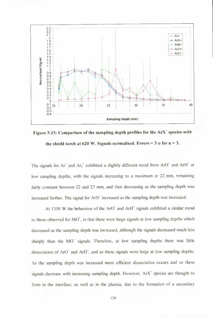
CO

t : o ft

23 22 21

2 19 18 17 16 15 14 1 3 12 11

1 4 09 08 07 06 0.5 04 03 02 0 1

0

ArH-f

• AfO • Ar2+

-01 -02 -03 -04

15 30 35

Sampling Depth (mm)

Figure 5.13: Comparison of the sampling depth profiles for the ArX* speeies with

the shield torch at 621) \N. Si<:nals normalised. Krrors = 3 a for n = 3.

The signals for Ar* and Ar2* exhibited a slightly different trend from ArO* and ArH* at

low sampling depths, with the signals increasing to a maximum at 22 mm, remaining

fairly constant between 22 and 27 mm, and then decreasing as the sampling depth was

increased tlirther. The signal for ArN* increased as the sampling depth was increased.

At 1350 W the behaviour of the ArO* and ArH^ signals exhibited a similar trend

to those observed for M O \ in that there were large signals at low sampling depths which

decreased as the sampling depth was increased, although the signals decreased much less

sharply than the MO* signals. Therefore, at low sampling depths there was little

dissociation of ArO* and A r H \ and so these signals were large at low sampling depths.

As the sampling depth was increased more efficient dissociation occurs and so these

signals decrease with increasing sampling depth. However, ArX* species are thought to

form in the interface, as well as in the plasma, due to the formation of a secondary

139

discharge behind the sampler cone. This secondary discharge, which promotes the

formation of ArX^, becomes more intense as the sampler is retracted further downstream

in the plasma*** . Therefore, due to an increase in the secondary discharge the ArX^

signals would be expected to increase as the sampling depth was increased, and this was

observed at sampling depths greater than 31 mm, where the ArO" and ArFT signals

began to increase again as the sampling depth was increased beyond 31 mm.

The Ar^ signal exhibited a trend similar to the metal analytes, although the

maximum signal occurred at a larger sampling depth than that exhibited for the metal

ions. At low sampling depths the short residence time in the plasma leads to insufficient

ionisation of the argon atom. As the sampling depth increases the Ar* signal increases,

due to more efficient ionisation. As the sampling depth is increased further less efficient

ionisation occurs at the lower temperatures at these sampling depths, and so the Ar*

signal decreases. The maximum Ar^ signal occurred at a larger sampling depth than the

metal ions due to its higher ionisation potential. The ionisation potential of Ar at 15.76

eV is almost double that of the metals studied, which are typically less than 8 eV, and so

a longer residence time in the plasma is required for effective ionisation of Ar to occur,

compared to that for the metals, resulting in a maximum signal at a larger sampling

depth.

The Ar2* signal followed an identical trend to that observed for the Ar* signal.

Ar2* is thought to be formed in the plasma by collisional reactions, rather than by

ionisation of the neutral species*^^ e.g.

Ar + Ar*<^ Arz' (5.1)

140

As the population of Ar' increases at increasing sampling depths, the Ar2^ signal would

increase as more collisional reactions with Ar occur within the plasma, and then decrease

again as less Ar* is formed in the plasma at greater sampling depths.

The signal for ArlsT exhibited a completely different trend to those exhibited by

the other ArX* species, with the signal increasing as the sampling depth was increased.

This can be explained by air entrainment. As the sampling depth was increased the

plasma was moved further away from the sampling cone, increasing the air entrainment

into the system.

At 620 W (Figure 5.12) the ArX* signals are similar to those exhibited at 1350

W. However, at large sampling depths (greater than 30 mm) the ArX" signals increase to

significant levels. This can be explained by the secondary discharge which becomes more

intense as the sampler is retracted further downstream in the plasma*** . Therefore, at

larger sampling depths the secondary discharge becomes more intense, promoting the

formation of ArX* species. This trend was also observed at 1350 W but was not so

pronounced due to the large ArX^ signals at low sampling depths. At 620 W the ArX*

signals were lower than those at 1350 W, due to the reduced plasma power, and so the

signals at larger sampling depths were of comparable intensity to those at low samphng

depths. At both 1350 W and 620 W a prominent secondary discharge was easily

observed at the tip of the sampler cone, especially at large sampling depths when the

secondary discharge was not obscured by the light emitted from the plasma. However, at

the power used with the shield torch (620 W) no secondary discharge was observed,

although a secondary discharge has been observed when using a shield torch at powers

above 1200 W^"

With the shield torch (Figure 5.13) the signals for ArO\ ArH* and ArlsT,

exhibited a similar trend, in that the signals remained fairly constant to a sampling depth

of 24 mm, before decreasing as the sampling depth was increased further. Unlike the

141

signals at 1350 W and 620 W the ArX* signals with the shield torch did not increase at

sampling depths above 30 mm, due to the removal of the secondary discharge which

causes this effect. The maximum signal observed occurred over a wider range of

sampling depths than at 1350 W and 620 W. With the shield torch the plasma potential is

greatly reduced and so effective dissociation of these species occurs at a greater sampling

depth. The signals for Ar* and Ar2* did not exhibit a determinable trend with sampling

depth, due to the reduced potential with the shield torch which was not sufficient to

effectively ionise the argon in the plasma.

Previous studies on argon polyatomic species are not as common as for the

metals or their oxides, and those that have been carried out are very patchy. Evans and

Ebdon*^^ investigated the effect of sampling depth (8.75 - 11.5 mm) on ArO*, ArN* and

Ar2^ at conditions comparable to those at 1350 W in this study. The signal for all of these

ions gradually increased as the sampling depth was increased. Kawaguchi et al also

investigated the effect of sampling depth ( 4 - 1 0 mm) on ArO" and Ar2* at 1200 W,

although it was only in the form of the effect of carrier gas flow rate at various sampling

depths. The signal for ArO* decreased as the sampling depth was increased, while the

signal for Ar2* increased as the sampling depth was increased, at a carrier gas flow rate

of 0.9 1 min'V Nonose ei ai investigated the effect of sampling depth (12 - 16 mm) on

ArO" with a shield torch at several different forward powers. At 800 W the signal for

ArO"*" increased to a maximum at 15 mm and then decreased as the sampling depth was

increased further. At higher powers the signal increased as the sampling depth was

increased, over the range of sampling depths studied.

Therefore, previous studies have found that argon polyatomic signals increased at

low sampling depths. However, all these studies were carried out at sampling depths

which were beyond the range of this study and so a valid comparison is not possible.

142

5.4 CONCLUSIONS

The sampling depth had a significant effect on the signal for metal analytes and

polyatomic ions, showing how important it is to optimise the sampling depth for

maximum response, and also to reduce interferences. At a sampling depth of 20 nmi the

analyte ion signal was two thirds of the signal at 16 mm. However, the metal oxide signal

at 20 mm had dropped to less than one tenth of the signal at 16 mm. Therefore, simply

by careful selection of the sampling depth it is possible to greatly reduce the metal oxide

interferences, with minimal loss of signal. This eliminates the need for other, more

expensive or time consuming, methods for oxide reduction, such as desolvation.

However, this is not effective for the argon polyatomic species, which are still present in

the plasma in significant amounts at sampling depths beyond 25 mm.

These argon polyatomic species are greatly reduced, in most cases to negligible

levels, with the use of the shield torch, while maintaining a reasonable level of metal

analyte signal. Unfortunately, with the shield torch the levels of metal oxides greatly

increased, especially at sampling depths up to 25 mm. This difference in behaviour

between the metal oxides and argon polyatomics, with the shield torch, suggests that

they may be formed by different mechanisms*'* . This can also be seen in the temperatures

calculated for the different species, where temperatures of 5000 - 14,000 K suggest that

metal oxides are formed in the plasma, and temperatures below 1500 K suggest that

argon polyatomics are formed in the interface region of the plasma. The use of

temperature calculations to investigate the possible site of formation for interference ions

is investigated in a later chapter.

The presence of the secondary discharge has a great influence on both the raw

signals and the dissociation temperatures. While the signals for both the metal oxides and

the argon polyatomics decrease with increasing sampling depths, at sampling depths

greater than 30 mm the ArX^ signals at 1350 W and 620 W began to increase again. At

143

these sampling depths the region of the plasma being sampled is beyond the tail plume,

and so it is the secondary discharge which is being sampled. The secondary discharge

promotes the formation of ArX* species and this was observed at sampling depths above

30 mm, where the ArX* signals increased as the sampling depth was increased. With the

shield torch, where no secondary discharge is formed, the ArX* signals did not increase

at sampling depths greater than 30 mm.

The temperatures calculated for both the metal oxides and argon polyatomic

species increased as the sampling depth was increased, at both 1350 W and 620 W. At

both 1350 W and 620 W a prominent secondary discharge was observed at the tip of the

sampler cone, which becomes more intense as the sampler is retracted further

downstream in the plasma'** . As the sampling depth was increased the secondary

discharge would increase, resulting in an increase in the plasma potential. An increase in

the plasma potential would increase the energy coupling to the plasma, resulting in an

increase in temperature. Therefore, although the temperature would be expected to

decrease with increasing sampling depth, the increased secondary discharge resuhs in an

increase in temperature with increasing sampling depth at 1350 W and 620 W. With the

shield torch no secondary discharge was observed, and the temperature decreased with

increasing sampling depth as expected.

In this investigation the minor isotopes of many of the species studied were used

in order to prevent the overloading of the detector. However, it was found that although

the minor isotopes gave ample signal at 1350 W this was not always the case. At 620 W

and with the shield torch the signals for some species dropped significantly, especially at

larger sampling depths. While these greatly reduced signals could still be used to

calculate the temperature, it would introduce unnecessary errors into the temperature

calculation. In the case of Ar* the signal with the shield torch was so low that it was not

possible to calculate the temperature. Therefore, in all further experiments more major

144

isotopes of the analytes under investigation will be used, in order to prevent these errors

in the temperature calculations.

The shield torch was operated with compromise conditions, so that while the

argon polyaiomics were reduced there was also some loss of analyte signal, by about an

order of magnitude. Throughout the experiment it was impossible to reduce the argon

polyatomic species further without reducing the metal ion signal to lower than this

recommended amount. The shield torch was operated at 620 W because that was the

default power setting which the plasma was set at when the shield was in operation.

Therefore, it was assumed that since that was the default power setting that it was also

the optimum power at which the shield torch operated. However, subsequent

investigations revealed that the plasma was not stable with the shield torch at the

recommended power of 620 W, so further experiments were performed at 700 W.

145

CHAPTER 6

Effect of Power on Polyatomic Ions and their

Dissociation Temperatures

146

6 E F F E C T OF POWER ON POLYATOMIC IONS AND

T H E I R DISSOCIATION TEMPERATURES

6.1 INTRODUCTION

Plasma operating conditions, such as nebuliser gas flow rate, power and solvent

loading, influence the relative positions of the initial radiation zone (IRZ) and normal

analytical zone (TSIAZ), and are thus related to the sampling position '* . I f the RF power

is increased, the IRZ and NAZ move closer to the load coil because the central channel

of the ICP contracts^^. Therefore, at a fixed sampling depth, increasing the RF power

moves the sampling region of the ICP from the IRZ to the NAZ^ '*** . As shown in

Chapter 5, the sampling position greatly affects the signal obtained for both metal analyte

species and polyatomic ion interferences. Therefore, it would be expected that plasma

operating conditions which are related to the sampling depth would also affect the

signals of metal analyte ions and polyatomic ion interferences.

6.2 EXPERIMENTAL

Experiments were conducted using a PlasmaQuad 3 (VG Elemental, Ion Path,

Road Three, Winsford, Cheshire, UK), as described in Section 2.1.2. Both ArX* and

MO* interferences were studied at the m / z shown in Table 6.1.

A power profile of the plasma was obtained from 550 to 1600 W at 50 W

intervals, at a sampling depth of 16 mm. When using the shield torch the power profile

was obtained from 650 to 1400 W at 50 W intervals, due to the unpredictable stability of

the plasma with the shield torch at lower powers and the possibility of damaging the Ni

147

shield with prolonged use at high powers. At each power monitored all other operating

parameters, i.e. lens settings and position of torchbox were adjusted to give maximum

signal for *'^ln*.

Table 6.1: Isotopes studied during effect of power experiment


A l ' 27 100 Ar2^ 80 99.2

Ar^ 36 0.34 r 89 100

ArH" 39 0.1* Zr^ 90 51.4

AID* 43 99.8* YO^ 105 99.8*

Ti^ 48 73.8 ZrO' 106 51.3*

ArN" 54 99.2 In^ 115 95.8

M n ' 55 100 Ba^ 138 71.7

ArO^ 56 99.4* La^ 139 99.9

TiO^ 64 73.6* BaO* 154 71.6*

MnO' 71 99.8* LaO* 155 99.7*



6.3.1 Variation of Dissociation Temperature with Power

6. J . /. 1 Dissociation Temperature of MO*

The methods used for calculating the dissociation temperature of the metal oxides

have been described previously for Methods A and B in Sections 4.3.2.1 and 4.3.2.2,

respectively.

148

Comparisons of the dissociation temperatures, using Methods A and B,

calculated for the different metal oxide species with standard conditions and with the

shield torch are shown in Figure 6.1.

18000

16000 i

14000

12000

10000

8000

6000

4000

2000

Standard (Method A) Standard (Method B) Shield Torch (Method A) Shield Torch (Method B)

500 — h -700 900 1100

Power (W) 1300 1500 1700

Figure 6.1: Comparison of the efTect of power for the MO^ temperature.

Errors = 3 a f o r n = 3.

With standard conditions the metal oxide dissociation temperatures increased as

the power was increased. The temperature calculated using Method A increased from

7900 K at a power of 550 W to 16,500 K at 1600 W, while the temperature calculated

using Method B increased from 6000 K at a power of 550 W to 10,500 K at 1600 W.

The temperatures calculated at higher powers using Method A were higher than the

range expected within the plasma (4000 - 10,000 K ) " \ but the temperatures calculated

using Method B were within this range expected within the plasma.

As the power was increased more energy would enter the plasma and so the

temperature within the plasma would increase. Therefore, the temperature would be

149

expected to increase as the power was increased. Longerich^*'* and Grain et a/.^" have

investigated the effect of power on the dissociation temperature of metal oxides and the

ionisation temperature of Sb and As, respectively. They found that the temperature

increased as the power was increased.

With the shield torch the temperatures initially decreased as the power was

increased but then remained fairly constant as the power was increased above 800 W.

The temperature calculated using Method A decreased from 5650 K at a power of 650

W to 4250 K at 850 W, while the temperature calculated using Method B decreased

from 4500 K at a power of 650 W to 3150 K at 850 W. At powers above 800 W the

temperature with the shield torch remained fairly constant as the power was increased.

Previous studies ** have shown that the plasma potential with the shield torch varies

much less with the plasma operating parameters than with a standard coil. Therefore, the

power has little effect on the plasma potential, and hence the temperature, with the shield

torch.

The temperatures calculated with the shield torch were lower than those

calculated with standard conditions. This would be expected because the use of the

shield torch removes the capacitive coupling and the secondary discharge within the

plasma, removing some of the energy within the plasma. Therefore, with less energy

within the plasma the temperature would be expected to be lower.

6.3. L 2 Dissociation Temperature of ArX"

This method for calculating the dissociation temperature of the argon polyatomic

ions has been described previously for Method E in Section 4.3.2.5.

The power profile of the temperature for ArO* is shown in Figure 6.2. These

results show that the temperature for ArO" with standard conditions increased from 480

K at 550 W to a maximum of 830 K at 1100 W. The temperature then decreased to 700

150

K at 1200 W, af^er which the temperature varied very little as the power was increased

further. With the shield torch the temperature increased from 500 K at 650 W to a

maximum of 830 K at 1350 W. As the power was increased more energy would enter the

plasma and so the temperature within the plasma would increase. Therefore, the

temperature would be expected to increase as the power was increased.

900

800

700

600

500

400

300

200

100

Standard (Plasma) Standard (Interface) Shield Torch (Plasma) Shield Torch (Interface)

500 700 900 1100 Power m

1300 1500 1700

Figure 6.2: Comparison of the effect of power for the ArO* temperature. Errors =

3 a f o r n = 3.

The temperatures calculated with the shield torch were slightly lower than those

calculated with standard conditions. This would be expected because the use of the

shield torch removes the capacitive coupling and the secondary discharge within the

plasma, removing some of the energy within the plasma. Therefore, with less energy

within the plasma the temperature would be expected to be lower.

151

Argon polyatomics, such as ArO\ are thought to possibly be formed in the

interface rather than in the plasma''*^ and this may reflect the low temperature. The


plasma. With standard conditions the temperature for ArO* in the interface increased

from 300 K at 550 W to a maximum of 420 K at 1100 W. The temperature then

decreased to 380 K at 1200 W, after which the temperature varied very little as the

power was increased further. With the shield torch the temperature increased from 300 K

at 650 W to a maximum of 415 K at 1350 W.

These temperatures calculated for both the plasma and interface are much lower

than expected for the plasma. The temperature calculations are based on p - LTE

conditions within the plasma, and therefore the such low temperatures calculated using

ArO^ may indicate a deviation from LTE conditions. LTE conditions are not thought to

exist in the interface region of the ICP - MS, suggesting that the ArO^ species is formed

in the interface rather than the plasma. The low temperatures calculated correspond to

those thought to prevail in the interface (< 3500 K)^''^ also suggesting formation in the


6.3.2 Effect of Power on Signal

The metal ion signals with standard conditions increased as the power was

increased, as shown in Figure 6.3 for La^ although the signal was negligible below 1050

W. With the shield torch the signal for La^ was negligible at all powers, although the

signal increased as the power was increased.

152

1400000

1200000

1000000

S. 800000

n ^ 600000

400000

200000

Standard Shield Torch

500 700 900 1100

Power (W)

1300 1500 1700

Figure 6.3: Effect of power on the signal for La*. Errors = 3 a f o r n = 3.

All the metal ions studied, as given in Table 6.1, exhibited the same trend with

standard conditions, with the signals increasing as the power was increased. This trend

would be expected, because as the power was increased there would be more energy

available within the plasma to ionise analytes present in the plasma. As the power was

increased an increase in analyte ionisation would therefore lead to an increase in metal

ion signal.

With the shield torch all of the metal ions studied also increased as the power was

increased, with several species reaching a maximum signal and then decreasing as the

power was increased further. However, not all the metal ion signals v^th the shield torch

were negligible in comparison to those with standard conditions. The signals for A l ^

Mn* and the internal reference ion In* exhibited a different trend to that observed for La*,

as shown in Figure 6.4 for Al*. The signal for Al* with the shield torch was much greater

than that with standard conditions. This was particularly pronounced at powers below

153

1100 W, where the signals with the shield torch were more than ten times greater than

the signals with standard conditions. Even at high powers the signals with the shield

torch were twice that of the signals with standard conditions.

4500000

4000000

3500000

3000000

g- 2500000 4

I 2000000 to

1500000 4

1000000

500000-i-

Standard Shield Torch

.i

500 700 900 1100 Power (W)

1300 1500 1700

Figure 6.4: Effect of power on the signal for Ar, Errors = 3 CT for n = 3.

The signal with the shield torch would be expected to be lower than with

standard conditions, since the plasma would be cooler with the shield due to the removal

of the capacitive coupling and secondary discharge within the plasma. Therefore, at the

same operating power there would be less energy within the plasma to ionise metal

analytes and so there would be less signal with the shield torch.

The difference in NT signal with the shield torch could possibly be explained due

to the oxide forming potential of the metal analytes. La readily forms oxides, the

promotion of which with the use of the shield torch, was shown in Section 5.3.3.

Therefore, due to the high probability of oxide formation with the shield torch, the signal

for La^ would be expected to be small since any La present in the plasma would form

154

LaO\ In addition the reduced energy with the shield torch does not promote the

dissociation of the oxide, due to the high dissociation energy of this species, resuhing in

large LaO" signals. However, metals such as In, AJ and Mn form oxides less readily than

La, hence giving rise to higher signals with the use of the shield torch.

Previous studies on the effect of power on metal analyte species include Li"^

134.136,138 g+ 136,137 137 134,136,137 134,137 j j * 136,137 y+ 137 136,137 137,150

137 ^ ^ + 134.137-139.150 | ^ | * 136.137 »37 139 { b 137 § g + 2 8 1 130,134.138,139.150.314

Pb^ 136.137,139,150^ 125.134,150,304^ p^. 136^ p j . 136^ 136^ 136^ 136^ 136^ j ^^+ 136,150^

HT In^ Sn^ Sb' TV Bi^ Sr i T La^ B e ^ a n d

Cs" These have found that the signal for metal analytes, with standard conditions,

increased as the power was increased, ahhough one investigation*^^ found that a

maximum in signal was reached depending upon the mass of the analyte. These findings

correspond to the resuhs of this investigation, where with standard conditions the metal

analyte signals increased as the power was increased.

Sakata et o/.*" investigated the effect of power on Co" , with the use of a shield

torch. They found that the signal for Co* increased as the power was increased. This

corresponds to the findings of this investigation, where the signals for the metai analytes

increased as the power was increased.

6.3.3 Eflect of Power on MO"^ Signal

An example of the effect of power on metal oxide signals is shown in Figure 6.5

for LaO^ These results show that with standard conditions the signal for LaO^ increased

as the power was increased. With the shield torch the signal for LaO* increased as the

power was increased. The signal for LaO^ with the shield torch was much greater than

that with standard conditions, particularly at powers above 900 W. The signal for LaO*

155

would be expected to decrease with increasing power^^, due to more effective

dissociation of the metal oxide with increasing power^^^

1600000

1400000

1200000 +

1000000

•5 800000 c w

600000

400000

200000 4-

standard • • • Shield Torch

500 700 900 1100

Power (W)

1300 1500 1700

Figure 6.5: EfTect of power on the signal for LaO" . Errors = 3 o for n = 3.

Metal oxide signals are more commonly expressed as a MO" / M^, and these MO^

/ ratios are shown in Figures 6.6 and 6.7 for standard conditions and with the shield

torch respectively.

These results show that with standard conditions the MO^ / ratio decreased,

for all the species studied, despite the raw MO^ signal increasing with increasing power.

At low powers there was less energy within the plasma to dissociate the metal oxide

while, at high powers there was more energy within the plasma and so the metal oxides

were more effectively dissociated.

156

4500

4000

3500

_ 3000

2500

i 2000

Power (W)

—•— LaO* (Do = 8.88eV)

• Z f O (Do = 776eV)

YCH (Do = 7 24eV)

TiO+ (Do = 6 93eV)

—•— BaO+ (Do = 4 09eV)

MnO* (Do = 2.75eV)

AID* (Do = 1.71eV)

1300 1500 1700

Figure 6.6: ( omparison of the effect of power for the MO* / IM* ratio with

standard conditions. MO* and M* signals normalised to 100%. Molecular and

atomic abundances are given in Table 6.1. Do values given are for MO*.

900000

800000

700000

_ 600000

I 500000

5 400000

6

* 300000

200000

100000

LaCK (Do = 8 88eV) ZsO* (Do = 7 76eV) Y D * (Do = 7 24eV) TiO+(Do = 6 93eV) BaO+ (Do = 4 09eV) MnO^ (Do = 2 75eV) A l O (Do = 1 71eV)

600 1500

Figure 6.7: Comparison of the effect of power for the MO* / M* ratio w ith the

shield torch. M O ' and M ' signals normalised to 100V«. Molecular and atomic

abundances are given in Table 6.1. Do values given are for MO .

157

Comparisons of the MO* / M* ratios show that the MO* / M* ratio increased as

the dissociation energy of the metal oxide increased. Species with a large dissociation

energy require large amounts of energy to break the metal oxide bond, so were persistent

in the plasma, and a large signal was therefore observed in relation to the metal signal,

resulting in a large MO* / M* ratio. Conversely, species with low dissociation energies

require little energy to break the metal oxide bond, were less persistent in the plasma, so

relatively little signal was observed in relation to the metal signal, resulting in a small

MO* / M* ratio. At low powers the MO* / M* ratios were extremely high, greater than

50 % for all species except Al and Mn, and several of these were much greater than 100

% (i.e. the oxide signal was greater than the metal signal). It was only at powers above

1200 W that the MO* / M* ratios dropped below 10 %, and even at the highest powers

the MO* / M* ratio for La did not fall below 5 %.

With the shield torch the MO* / M* ratios were different to those exhibited with

standard conditions, and did not exhibit the same trend as each other, as shown in Figure

6.7. These results show that, with the exception of Al and Mn, the MO* / M* ratios were

much higher than those with standard conditions. The MO* / M* ratio for Al and Mn

remained fairly constant with the increase of power, while the MO* / M* ratio for Ba

decreased as the power was increased. For all other species the MO* / M* ratio increased

as the power was increased, with Ti and Y reaching a maximum at about 1000 W and La

and Zr reaching a maximum at a power of about 1300 W.

The shield torch greatly promoted the formation of the metal oxides, well beyond

the level which would be expected, and this is particularly prominent at high powers. At

high powers the MO' / M* ratios with standard conditions were negligible, due to

increased dissociation of the metal oxide at these higher powers. With the shield torch

the plasma is cooler than v^th standard conditions, and the metal oxides are not so

158

effectively dissociated at these lower temperatures, resulting in greater MO" / ratios,

particularly at higher powers.

Previous studies on the effect of power on metal oxide species have been

performed, using standard conditions, on CeO^ BaO' TbO^ GdO*

ThO^^^ and LaO^ In all cases it was found that the M O ' / ratio decreased as the

power was increased, as found during this investigation for standard conditions.

6.3.4 Effect of Power on ArX^ Signal

An example of the effect of power on ArX' is shown in Figure 6.8 for ArO" .

These results show that the signal for ArO^ increased to a maximum at 650 W and then

decreased as the power was increased up to 1100 W. Beyond 1100 W the signal rose

until a power of 1250 W, after which the signal remained fairly constant.

4500000

500 700

4000000 +

3500000 +

3000000 +

J 2500000 4-

5> 2000000

1500000 +

1000000

standard Shield Torch

900 1100 Power (W)

1300 1500 1700

Figure 6.8: Effect of power on the signal for ArO*. Errors = 3 o for n = 3.

159

The signals for the argon polyatomic species would be expected to increase as

the power was increased, as more energy is introduced into the plasma promoting the

formation of argon polyatomic species. At powers above 1100 W the ArO" signals

followed this expected trend, in that the signals increased as the power was increased.

However, at powers below 1100 W the ArO* signal increased as the power was

decreased below 1100 W. This can be explained by the formation of the secondary

discharge, which is strongest at low powers*^ . The secondary discharge, which

promotes the formation of argon polyatomic species*^^ is correlated with the plasma

potential, which has been found to be three times higher at 800 W than 1400 W^°^.

Therefore, this increase in plasma potential, and hence secondary discharge, at low

powers would be expected to enhance the ArX* signals at low powers.

With the shield torch the signal for ArO" increased as the power was increased

until 1000 W. Beyond 1000 W the signal decreased as the power was increased further,

until a power of 1300 W, after which the signal began to increase again. The ArO* signal

could initially increase as the power was increased, due to the increased ionisation of O

precursors from the nebuliser gas, resulting in an increased signal*^ . However, ArO" has

very low dissociation energies (0.4 eV) compared to the ionisation potentials of its

constituent species (14 eV), hence as the power was increased further the dissociation of

ArO* would become the predominant effect. However, at powers above 1300 W the

signals began to increase again with a further increase in power. Sakata et al. observed

that even with the use of the shield torch the secondary discharge was present in the

plasma at powers above 1200 W. Therefore, this increase in ArO" signal above 1300 W

could be due to the secondary discharge reappearing in the plasma, which promotes the

formation of ArX^ species. The signal with the shield torch was negligible compared to

that without the shield.

160

The effect o f power, with standard conditions, on various ArX* species, as given

in Table 6.1, is showTi in Figure 6.9. These resuhs show that the signals for ArFT, ArN*,

and ArO* all showed a similar trend, ahhough the effect was much more pronounced for

ArO*, while the signals for Ar*, and AT:* exhibited a similar trend, with the signals

increased as the power was increased. The signal for Ar* would be expected to be similar

to those observed for metal analyte species because although the plasma is composed of

argon, only about 0.1 % is ionised^\ In addition, argon is introduced into the plasma in

the same way as analyte species in the form of the nebuliser gas. Therefore, as the power

was increased the Ar would be more efficiently ionised, leading to an increase in Ar*

signal.

Power (W)

Figure 6.9: C omparison of the effect of power for the ArX* species with standard

conditions. Signals normalised. Errors = 3 CT for n = 3.

Ar2* is thought to be formed in the plasma by collisional reactions, rather than by

ionisation of the neutral species' , e.g.

161

AT + AT* <^ Arz (6.1)

As the population of Ar* increased at high powers the Ar2* signal would be expected to

increase as more collisional reactions with Ar occur within the plasma.

The effect of power, with the shield torch on various ArX* species is shown in

Figure 6.10. The signals for A r H \ and ArN* exhibited a trend similar to that observed

for ArO'. With the shield torch the signal for Ar' exhibited the same trend as that shown

with standard conditions, in that the signal increased as the power was iiKreased.

I hcrclorc. both with and without the shield torch Ar exhibited the same trend as the

metal analytes introduced into the plasma.

Power W

Figure 6.10: Comparison of the effect of power for the ArX^ species with the shield

torch. Signals normalised. Errors = 3 a for n = 3.

162

The signal for ATJ* increased to a maximum at 900 W before decreasing as the power

was increased further. I f Ar2* was formed according to Equation 6.1 the Ar2* signal

would be expected to increase as the power was increased, as more Ar was ionised.

However, the dissociation energy of Ar2* is very low (1.05 eV), and so as the power was

increased further the dissociation of Ar2^ would rapidly become the predominant process

occurring within the plasma, leading to a decrease in the Ar2^ signal.

Previous studies on the effect of power on ArX* have mainly investigated the

effect of power with standard conditions. Gray and Williams* '* and Kawaguchi et aL^^

investigated the effect of power (1.1 - 1.5 kW) on Ar2^ and ArO*. They both found that

the signal for Ar2' increased as the power was increased. Gray and Williams' ** also found

that the signal for ArO^ increased as the power was increased. However, Kawaguchi et

a/.'**** found that the ArO" signal decreased as the power was increased, to a power of

1300 W and then increased slightly as the power was increased further. Evans and

Ebdon*^^ also investigated the effect of power (1.0 - 1.8 kW) on A r O \ ArK", and Ar2' .

They found that the signals for ArO* and ArN* decreased as the power was increased,

while the signal for Ar2' varied little over the range studied. Therefore, none of the

previous studies have investigated the effect of power below 1000 W. However, they

found that the signals for all the ArX^ species increased as the power was increased* ** '****,

as expected, and as seen in this study at powers above 1100 W.

Sakata et <7/.*" and Nonose et a/.*** investigated the effect of power (0.7 - 1.4

kW) with the use of the shield torch on A r \ Axi, ArO* and ArH". They found that the

signals for Ar* Ar2* and ArO* increased as the power was increased,

although the signals were negligible below 1.2 kW*^ . The signal for ArH" was much

larger and exhibited a different trend to that shown by the other argon polyatomic

species*". The signal for ArH" increased as the power was increased up to a power of

0.9 kW, after which it decreased as the power was increased further up to a power of 1.2

163

kW. Beyond 1.2 kW the signal began to increase again as the power was increased

further. Therefore, although the results from this study differed from most o f the

previous studies, they did follow a similar trend to that seen by Sakata et al. for ArH*.

6.4 CONCLUSIONS

The operating power had a great effect on the signals for metal analytes and

polyatomic ions. With standard conditions the metal analyte signals were negligible at

powers below 1100 W, showing how important it is to operate at a high enough power

to ionise the analytes of interest. However, at these higher powers polyatomic ion signals

were also higher, although the MO* / NT ratios were lower at high powers.

The use of the shield torch effectively reduced the argon polyatomic ion species,

particularly at high powers. The use of the shield torch also significantly enhanced the

signal for certain metal analytes, at all powers. Therefore, the use of the shield torch at

high powers significantly reduces the argon polyatomic species and also increases analyte

sensitivity by at least double. However, the formation of metal oxides was greatly

enhanced with the shield torch, particularly at high powers, and this is reflected in the

low signals for the metal analytes, such as La, which readily form oxides.

Therefore, while the operation of the shield torch at high powers has significant

potential for both increased analyte sensitivity and removal of interferences, the nature of

the analyte being studied must be carefully considered, with oxide forming analytes

causing a specific problem. Not only is the sensitivity of these species greatly reduced

with the shield at high powers, but the formation of oxide species may cause interference

problems on other analytes being studied.

164

CHAPTER 7

Effect of Solvent Loading on Polyatomic Ions and their

Dissociation Temperatures

165

7 E F F E C T OF SOLVENT LOADING ON POLYATOMIC

IONS AND T H E I R DISSOCIATION TEMPERATURES

7.1 INTRODUCTION

Samples are most commonly introduced into an ICP by aspiration of aqueous

samples in the form of an aerosol, which is a mixture of gases, droplets, particles and

solvent vapour, although gaseous sample introduction is also possible.

Water vapour introduced into the plasma region influences the coupling of the

plasma with the RF field, which in turn affects the power absorbed by the plasma^* .

Water dissociation must also be taken into account as this process requires a large

amount of energy^^, hence, this would lower the amount of energy available for analyte

atomisation and ionisation '*^ In addition, the power required to desolvate aerosol

droplets, atomise solvent molecules and then excite the solvent pyrolysis products is

supplied at the expense of the power available to vaporise, atomise and excite the

analyte '*^ Therefore, the solvent loading of the plasma may greatly affect the energy

within the plasma available to ionise the analyte species. It has been proposed that the

influence of variations in water aerosol loadings on plasma properties is substantially

greater than that of water vapour'** , because, for a certain water loading containing both

liquid aerosol droplets and water vapour, energy is required to vaporise the liquid

droplets before atomisation and ionisation of the resulting vapour can be achieved. This

should result in a significant difference in the intensity of both analyte and interference

signals for samples consisting of nebulised droplets and vapour, and vapour only,

particularly at similar solvent loadings.

166

Many of the most serious polyatomic interferences in ICP - MS are caused by

species which contain oxygen in combination with another element ** *^ '*". The presence

of water when aspirating aqueous samples is a major source of oxygen in the plasma, and

hence also oxygen containing interferences. Therefore, the introduction of the sample as

a vapour rather than as vapour / droplets should reduce the solvent loading, by removing

the droplets, and so should also reduce the amount of oxygen containing interferences.

7.2 EXPERIMENTAL


Ion Path, Road Three, Winsford, Cheshire, UK), as described in Section 2.1.2. Water

vapour was introduced directly into the back of the ICP torch using the apparatus shown

in Figure 7.1.

From Argon Supply

Mass Flow Controller OflCP-MS Nebuliser Gas

Rotameter

TolCP-MS < '

Dreschel Bottle

Sample

Figure 7.1: Schematic diagram of apparatus used for the introduction of water

vapour via a temperature controlled Dreschel bottle.

167

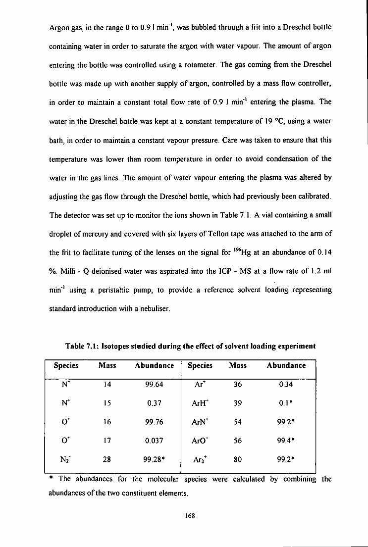
Argon gas, in the range 0 to 0.9 I min'*, was bubbled through a frit into a Dreschel bottle

containing water in order to saturate the argon with water vapour. The amount of argon

entering the bottle was controlled using a rotameter. The gas coming from the Dreschel

bottle was made up with another supply of argon, controlled by a mass flow controller,

in order to maintain a constant total flow rate of 0.9 1 min"* entering the plasma. The

water in the Dreschel bottle was kept at a constant temperature of 19 °C, using a water

bath, in order to maintain a constant vapour pressure. Care was taken to ensure that this

temperature was lower than room temperature in order to avoid condensation of the

water in the gas lines. The amount of water vapour entering the plasma was altered by

adjusting the gas flow through the Dreschel bottle, which had previously been calibrated.

The detector was set up to monitor the ions shown in Table 7.1. A vial containing a small

droplet of mercury and covered with six layers of Teflon tape was attached to the arm of

the frit to facilitate tuning of the lenses on the signal for *^Hg at an abundance of 0.14

%. Milli - Q deionised water was aspirated into the ICP - MS at a flow rate of 1.2 ml

min'^ using a peristaltic pump, to provide a reference solvent loading representing

standard introduction with a nebuliser.

Table 7.1: Isotopes studied during the effect of solvent loading experiment


14 99.64 Ar* 36 0.34

15 0.37 ArH* 39 0.1*

0* 16 99.76 ArN* 54 99.2*

0^ 17 0.037 ArO* 56 99.4*

28 99.28* A r / 80 99.2*



168


7.3.1 Effect of SoKent Loading on Dissociation Temperature

This method for calculating the dissociation temperature of the argon px)lyatomic

ions has been described previously for Method K in Section 4.3.2.5.

The effect of solvent loading on the dissociation temperature of AK)* is shown in

Figure 7.2.

^ 1000

• 1350W Plasma 1350W Interface

• 700W Plasma . 700W Interfaoe • Shiekj Rasma •• Shield Interface

Nebuliser

1 15 Sotvent Loading (g/hr)

2 5

Figure 7.2: Effect of solvent loading for the AK)* temperature.


These results show that at 1350 W the ArO* dissociation temperature in the

plasma increased as the solvent vapour loading was increased, from 750 K at a solvent

loading of 0.01 g / hr to 1550 K at a solvent loading of 0.94 g / hr. At 700 W the ArO*

dissociation temperature in the plasma also increased as the solvent vapour loading was

increased, from 350 K at a solvent loading of 0.01 g / hr to 900 K at a solvent loading of

169

0.94 g / hr. With the shield torch the ArO^ dissociation temperature in the plasma also

increased as the solvent vapour loading was increased, from 400 K at a solvent loading

of 0.01 g / hr to 600 K at a solvent loading of 0.94 g / hr. For all three conditions used

the temperature with the nebuliser was lower than that vAth the vapour.

As the solvent vapour loading was increased the amount of atomic hydrogen

entering the plasma would be increased. The thermal conductivity of hydrogen is about

ten times higher than that of argon^''\ and improves the heat transfer towards the central

channel"^ and so an increase in temperature would be expected. With the nebuliser the

solvent loading has increased, increasing the amount of atomic hydrogen entering the

plasma, and so the temperature would be expected to be greater than that with the

vapour. However, the temperature did not increase as the solvent loading was increased

with the nebulised droplets. The nebulised droplets introduced into the plasma require a

large amount of energy for vaporisation. This would reduce the energy within the

plasma, even though the presence of atomic hydrogen improves the heat transfer, and so

led to a reduction in the temperature calculated. Therefore, with the nebuliser, the

temperature decreased due to the extra energy required to vaporise the droplets.

Previous studies investigating the effect of solvent loading on the temperature

have been carried out by Alder et i?/."^ Tang and Trassy^**', and Murillo and Mermet^^

who investigated the effect of desolvation on the temperature. It was found that the

presence of water increased the temperature^^" ' **' by 1000 K^^.

For the ArO" dissociation temperature, calculated using equilibrium conditions in

the interface, the temperatures calculated were much lower than those calculated for the

plasma, at all three operating conditions used, but followed the same trends as those

shown by the temperatures calculated for equilibration in the plasma, (i.e. the

temperatures increased as the solvent vapour loading was increased, with the

temperature for the nebuliser being lower than for the vapour).

170


lower than expected for the plasma. The temperature calculations are based on p - LTE

conditions within the plasma, and therefore the low temperatures calculated using ArO^

may indicate a deviation from LTE conditions. LTE conditions are not thought to exist

in the interface region of the ICP - MS, suggesting that the ArO* species is formed in the

interface rather than the plasma. The low temperatures calculated correspond to those

thought to prevail in the interface (< 3500 K)'^'^, also suggesting formation in the


7.3.2 Effect of SoKcnt Loading on Polyatomic Ion Signals

The effect of solvent loading at 1350 W on the interference species studied, as

given in Table 7.1, is shown in Figure 7.3. These results show that as the solvent vapour

loading was increased the interference signals increased, reached a maximum at a solvent

loading of 0.7 g / hr and then decreased as the solvent loading was increased further.

Soh/ent Loading (g/hr)

Figure 7.3: Effect of solvent loading for the ArX* species at 1350 W. Signals

normalised. Errors = 3 a for n = 3.

171

With the increase in solvent vapour loading the signals would be expected to

increase, due to the increase in analyte mass transport^^^. However, as the vapour

loading was increased there would be more water vapour present in the plasma, which

would require more energy for atomisation, leading to less energy available within the

plasma for the ionisation of analyte species. This would lead to a decrease in signal at

higher vapour loadings.

The signal for species such as ArO*, and ArH* would be expected to increase as

the solvent vapour loading was increased due to an increase in the analyte mass

transport "* , which in this case is water. However, it was also found that the signals for

species such as Ar^, and Ar2^ also increase as the solvent vapour loading was increased,

even though they are not formed by any of the constituent species formed by the

atomisation of water. Hutton and Eaton'**^ also reported a strong dependence of the Ar2^

signal on the water loading. Therefore, the increased presence of water in the plasma not

only acts to increase the species which are directly formed from its constituent species,

but also it increases the signal of other species in the plasma.

The increase in solvent vapour loading introduces more atomic hydrogen into the

plasma, improving the heat transfer toward the central channel and leading to an increase

in temperature"^. This increase in thermal conductivity and temperature would explain

the strong dependence of signals such as Ar2' on the solvent loading, as more atomic

argon would be ionised, resulting in greater amounts of Ar2^ being formed. As v^th the

signals for ArO" , the signals would then begin to decrease as the solvent loading was

increased further due to the increase in water vapour, which would require more energy

to atomise.

With the nebuliser the signal for Ar* decreased compared to those for the vapour,

but the signals for the other ArX^ species increased compared to those v^th the vapour.

These signals would be expected to increase due to the much greater volume of solvent

172

entering the plasma as nebulised droplets compared to the vapour. With the nebuliser the

temperature was lower than for the vapour, and so the Ar^ signal would be expected to

be lower, due to a reduction in ionisation at the lower temperature with the nebuliser.

Previous studies investigating the effect of solvent loading have concentrated on

the reduction of the solvent loading by desolvation techniques ' **' *''**' * " , such as

membrane separators "'**'** or cryogenic desolvation^**'**", or the reduction of the

solvent loading by cooling the temperature of the spray chamber *'* ' ** . Several studies

have investigated the effect of aerosol water loading on the spectral characteristics

observed in ICP - MS by incrementally adjusting the spray chamber temperature^* ''* ' ***.

These studies found that the ArO* and Ar2^ signals were dependent on the solvent

loading*** , decreasing as the spray chamber temperature was reduced from 30 to 0 °C

(decreasing solvent loading). These species have also been investigated using desolvation

techniques ' ''**'* *'* '*'' ''*'* comparing signals with water present in the sample and

when the water had been removed from the sample. These studies showed that the

polyatomic ion interferences, such as ArO^, CIO^, ArCr and ArOtT were reduced when

the desolvation techniques were used **'" *'* .

Therefore, previous studies have found that interference ion signals decreased as

the solvent loading of the plasma was reduced.

The effect of solvent loading at 700 W and with the shield torch on the

interference species studied are shown in Figures 7.4 and 7.5 respectively.

These signals exhibited a similar trend to that observed at 1350 W, with the

signals increasing as the solvent vapour loading was increased, reached a maximum and

then decreased as the solvent vapour loading was increased further. At 700 W the signals

with the nebuliser were greater than those for the vapour, except for Ar*, due to the

greater volume of solvent entering the plasma.

173

12

Ar2-f ArH+ ArCK

N2+

1 15

Solvent Loading (g/hr)

Nebultser

2 5

Figure 7.4: Effect of solvent loading for the ArX* species at 700 W. Signals

normalised. Krrors = 3 a for n = 3.

to 0 8

05

. Ar+

• Ai2+

• ArH-f

• A f O

. ArN+

1 1.5 Solvent Loading (g/hr)

h4ebuliser

2 5

Figure 7.5: Effect of solvent loading for the ArX* species with the shield torch.

Signals normalised. Errors = 3 a for n = 3.

174

With the shield torch the signals with the nebuliser were lower than those for the vapour.

The temperature with the shield torch was lower than at 1350 W and 700 W and so, the

large amount of energy required to vaporise the droplets would reduce the energy

available for ionisation of the analytes, resulting in a decrease in signal with the nebuliser

compared to the vapour.

The signals at 1350 W were greater than those at 700 W, with the signals using

the shield torch being negligible compared with both these signals. This reflects the

amount of energy within the plasma, at each of these conditions, available to vaporise the

solvent and ionise analyte species.

7.4 CONCLUSIONS

The introduction of solvent in the form of nebulised droplets, compared with a

vapour, affected both the raw ArX"^ signals and the temperature calculated from them.

With the nebuliser the ArX" signals were greater than those for the vapour, due to the

increased volume of solvent entering the plasma. The introduction of solvent as nebulised

droplets reduced the temperature within the plasma, compared with that for the vapour,

due to the increased energy required to vaporise the water droplets. This reduction in

temperature would result in less energy available within the plasma to ionise analyte

species, ahhough this is not the case for the argon polyatomic species.

The introduction of solvent in the form of a vapour rather than as nebulised

droplets reduced the interference signals and increased the temperature of the plasma,

which would improve analyte signals. Therefore, i f the nature of the sample allows, the

introduction of the sample as a vapour would be beneficial, both due to the reduction in

interferences and the enhancement of analyte signals.

175

CHAPTER 8

Determination Of The Site And Mechanisms Of

Formation Of Polyatomic Ion Interferences

176

8 DETERMINATION OF T H E SITE AND MECHANISMS

O F FORMATION O F POLYATOMIC ION

I N T E R F E R E N C E S

8.1 INTRODUCTION

Since the development of ICP - MS, fiindamental studies have been performed to

elucidate ionisation and / or excitation mechanisms within the plasma^^^^^'^*'^. Analyte

ions are not the only species formed within the ICP, with molecular interference ions

such as oxides, hydroxides and background species due to plasma gases and / or solvent

being formed. These species can cause a significant problem and much work has been

carried out to reduce these interferences (as discussed in Section 1.2.2), however, the

mechanisms and site of formation of these interfering species are not well understood. A

clear interpretation of formation mechanisms and the site of formation of these

interfering species would greatly enhance the understanding of these interferences and

could lead to design modifications of the instrument, rather than relying on modification

of the analytical method, to reduce them.

One complication in the determination of the formation of polyatomic ions in ICP

- MS is related to the insertion of a sampling interface made of cooled metal between the

ICP and the mass spectrometer, and the resulting reactions occurring in the interface

region*'* . The secondary discharge occurring at the sampling region was thought to

affect the formation of M ^ ' and MO^ species*^°•*'*^•' '''* '' **' ^^ due to an increase in nc at

the surface of the sampling cone. However, this secondary discharge has been shown to

result from a large RF voltage swing in the plasma to the grounded interface ^**, and that

177

reduction in this plasma potential greatly affected the formation of ArX* species but had

little effect on M^* and MO^ formation"'*.

Therefore, comparison of the formation of polyatomic interferences and their

relationship to physical properties of the plasma with a standard plasma and with a shield

torch, which is known to affect the formation of polyatomic ions, may result in a better

understanding of the formation mechanisms and sites of formation of these species.

8.2 E X P E R I M E N T A L

Experiments were conducted using a PlasmaQuad 3 (VG Elemental, Winsford,

UK) using the experimental conditions described in Section 2.1.2.

Various solvents were introduced into the plasma at a flow rate of 1.2 ml min'*

using a peristaltic pump, including 2 % HNO3, 1 % methanol, 1 % HCl and 10 ng ml'*

MO solution. Various interferences were studied at the m / z shown in Tables 8.1 - 8.4.

Table 8.!: Isotopes studied during the introduction of 2 % HNO3 for the site of

formation experiment


>r 14 99.64 32 99.52*

15 0.37 Ar^ 36 0.34

16 99.76 Artr 39 0.1*

0 17 0.037 ArN" 54 99.2*

28 99.28* ArO* 56 99.4*

30 99.40* A r / 80 99.2*



178

Table 8.2: Isotopes studied during the introduction of I % HCI for the site of



c r 35 75.8 C I / 70 57.5*

Ar^ 36 0.02 ArCr 75 75.5*

ClO^ 51 75.6*

Table 8.3: Isotopes studied during the introduction of 1 % MeOH for the site of


Species IVfass Abundance Species Mass Abundance

12 98.9 Ar' 36 0.02

c / 24 97.8* ArC' 52 98.5*

CO' 28 98.7*

Table 8.4: Isotopes studied during the introduction of 10 ng ml'* MO Solution for

the site of formation experiment


A l ' 27 100 YO' 105 99.8*

AlO' 43 99.8* ZrO' 106 51.3*

T i ' 48 73.8 In^ 115 95.7

Mn" 55 100 Ba' 138 71.7

TiO^ 64 73.7* La* 139 99.9

MnO^ 71 99.8* BaO' 154 71.6*

r 89 100 LaO' 155 99.7*

Zr' 90 51.4



179

The experiment was carried out at 1350 W, 700 W and 700 W with a shield torch. With

each solvent studied the lens settings and torchbox position were adjusted to give

maximum signal for ''^In* prior to each analysis.


8.3.1 Temperature Determination

The methods for calculating the dissociation temperature of the metal oxide and

argon polyatomic ions have been described previously for Methods A, B and E in

Sections 4.3.2.1, 4.3 .2.2 and 4.3.2.5, respectively. The determination of the temperature

of molecular species XY*, i.e. CO^ required more complicated calculation since both the

constituent species were being introduced into the plasma. Also, the dissociation

mechanism is more complicated, since either species may form the positive ion, e.g.

CO* <^ C + O (8.1)

CO' <-> O' + C (8.2)

Therefore, the temperature was calculated using both possible mechanisms. The

concentration of the neutral species was calculated using Equation 8.3, using carbon in

methanol as an example.

density of C atoms = (((vapour loading / 3600) x % in solution x No) / (Molecular

weight X nebuliser gas flow)) x (Tbath / Tpiasma) (8.3)

180

This was then multiplied by the experimental O" / CO* ratio in order to obtain an

experimental (CO*) value, which could then be used to calculate the temperature

using the method described previously. Alternatively, the density of O atoms was

calculated using Equation 8.3, which was then multiplied by the experimental C* / CO*

ratio in order to obtain an experimental ¥^ (CO*) value, which was then used to calculate

the temperature.

The calculation of the temperatures for the species ArCI* and CIO* was not

possible due to the lack of available data for these ions, nor was it possible to calculate

the temperature for ArH*, due to the lack of data to calculate the partition function for

H*.

Polyatomic ions are thought to be formed in the interface as well as in the plasma,

and so the dissociation temperatures were calculated for equilibration in the interface as

well as in the plasma.

The dissociation temperatures calculated using this method are given in Table

8.5. These results show that at 1350 W the dissociation temperatures calculated for the

metal oxide ions ranged from 7350 - 9150 K, which correspond to the temperature

thought to prevail in the plasma. The MO* dissociation temperatures calculated at 700 W

were lower than those calculated for 1350 W, being in the range 5200 - 7900 K. This

would be expected due to the reduced power being introduced to the plasma, which

would result in lower plasma temperatures. The MO* dissociation temperatures

calculated with the shield torch were lower than the temperatures calculated at both

1350 W and 700 W. With the shield torch, not only was less power introduced into the

plasma, but the plasma potential was reduced, resulting in an even lower temperature.

181

Table 8.5: Dissociation temperatures calculated for the polyatomic ions (K)

1350W 700W Shield

Species Plasma Interface Plasma Interface Plasma Interface

ArO' ( 0 ^ 2245 584 828 415 2090 575

ArO'(ArO 867 424 619 356 726 388

Ar>r (N") 5222 2180 3148 1726 3810 1901

Ar>r(ArO 2544 1531 1500 1083 1076 835

4995 3890 3845 3157 2770 2395

ArC' (C^) 2795 1067 1505 814 4170 1202

ArC'(Ar') 1325 759 1405 785 1625 846

c / 4518 3174 4500 3165 3260 2500

CO' (0 ' ) 5423 4040 5020 3812 5121 3870

CO' ( C ) 3732 4803 5738 4277 5897 4364

C I / 4401 2831 3045 2205 3184 2276

M O ' 7368 5205 2752

(Kubota)

MO* 9145 7897 4355

(Longerich)

Due to the nature of the M O ' dissociation temperature calculation it was not

possible to calculate the temperature within the interface. However, the calculated M O '

dissociation temperatures show that they are probably formed in the plasma, with little

indication of formation in the interface.

The dissociation temperatures calculated for argon polyatomic species, such as

ArO', were much lower than those calculated for the metal oxides, with temperatures

below 2800 K, with the exception of ArlsT. Argon polyatomic ions are thought to be

182

formed in the interface rather than the plasma*'*^ and this may reflect the low

temperature. The temperatures calculated for the interface were even lower than those

calculated for the plasma, with temperatures in the range 400 - 2200 K. With a

dissociation temperature of less than 3000 K calculated at 1350 W it would seem

unlikely that the ArX" species were formed in the plasma, and this is reflected in the

dissociation temperatures calculated for the interface, which were generally less than

1000 K. This suggests that while there may be some ArX^ formed in the plasma, it is

predominantly formed in the interface.


lower than expected for the plasma. The temperature calculations are based on p - LTE

conditions within the plasma, and therefore the low temperatures may indicate a

deviation from LTE conditions. LTE conditions are not thought to exist in the interface

region of the ICP - MS, suggesting that the ArX^ species are formed in the interface

rather than the plasma.

ArN^, however, exhibited a different trend to the other ArX^ species, with a

dissociation temperature of 5200 K at 1350 W. This temperature corresponds to

temperatures thought to prevail in the plasma. However, the dissociation temperature

calculated for the interface was 2200 K, which is much less than thought to exist in the

plasma. Therefore, it is possible that ArN^ is formed in the plasma, probably due to air

entrainment, and also in the interface in the same way as the other ArX^ species.

Other polyatomic species, such as exhibit dissociation temperatures in the

range 3700 - 5500 K at 1350 W. These temperatures correspond to the temperature

thought to prevail in the plasma. The temperatures calculated for the interface are in the

range 2800 - 4800 K, which still correspond to temperatures within the plasma rather

than the interface. Therefore, this suggests than the other polyatomic species, such as

183

are formed in the plasma rather than in the interface like the argon polyatomic

species.

Polyatomic ions can be divided into two groups according to their formation

mechanisms, with argon polyatomic ions probably forming in the interface, and metal

oxides, and other species such as CO* and N2' probably forming in the plasma.

Previous studies into the formation mechanisms and site of formation of

polyatomic interferences are scarce. Nonose et a/.*'* theoretically calculated the

monoxide to analyte (MO / M) ratio, assuming the dissociation equilibrium in the ICP.

They proposed that the MO^ due to analytes was derived from undissociated MO in the

ICP because the theoretical MO / M ratios in the ICP agreed satisfactorily with the

experimental MO* / M" ratios. Similar calculations with ArO" showed little

relationship between the signal behaviour of ArO* and its dissociation equilibrium in the

ICP, suggesting that a collision - induced reaction of neutral argon and O^ was a

dominant process for the formation of ArO* Becker e/ a/}^^ investigated the

formation of several metal argide molecular ions, and from the similar distribution of

metal argide ions and metal ions they assumed that an association reaction was donunant

for their formation.

Nonose et al. '" ^ also carried out theoretical calculations to determine the site of

formation of various polyatomic ion species. The signal behaviour of MO" species

seemed to reflect the physical properties of the ICP rather than the interface, and was not

influenced by the secondary discharge occurring at the tip of the sampling cone.

Theoretical calculations were used to determine the equilibrium dissociation temperature

for ArO' and ArH ' The theoretical ArH^ / ArO* ratio which corresponded to the

experimental ratio produced a temperature of 3500 K, suggesting that the dissociation

equilibrium for ArX^ species was reached in the interface region of the ICP.

184

Therefore, previous studies into the site and mechanisms of formation for

polyatomic ions suggest that they can be divided into two groups. Metal oxide ions seem

to be formed in the ICP by the ionisation of undissociated MO in the ICP. Argon

polyatomic species, however, seem to be formed in the interface by collision - induced

reactions of neutral Ar with X".

8.4 CONCLUSIONS

Comparison of the dissociation temperatures calculated for different polyatomic

molecular ions shows that there was a wide range of temperatures determined,

depending on the molecular ion used for the calculation.

Dissociation temperatures calculated for metal oxide ions, at 1350 W were within

the range expected for the plasma. It was not possible to calculate the MO" dissociation

temperature in the interface, but there was little to suggest that metal oxide ions are

formed in the interface. Therefore, the dissociation temperatures calculated for the metal

oxide ions indicate that they are formed in the plasma.

Dissociation temperatures calculated for argon polyatomic species were much

lower than both those calculated for the metal oxides and those expected in the plasma,

with the temperatures calculated for the interface even lower than those calculated for

the plasma. This suggests that the argon polyatomic ions are not present in the plasma,

but formed within the interface. These low temperatures calculated for the ArX^ ions,

both in the plasma and the interface, suggest a deviation from LTE conditions, further

indicating formation in the interface, where LTE conditions are thought not to prevail.

The exception to this was ArN^, for which the dissociation temperature at 1350

W suggests formation in the plasma. A likely source of ArlsT is air entrainment, which

would result in the formation of Ar>r in the plasma. However, the ArN^ dissociation

185

temperature calculated for the interface was much lower than both that calculated for the

plasma and that expected within the plasma, suggesting that AiN^ was formed in the

interface in a similar method to the other ArX^ ions. Therefore, the dissociation

temperatures for ArN* suggest that it is formed both in the plasma and the interface.

Dissociation temperatures calculated for other polyatomic ion species, such as

CT", and CO^, for both the plasma and interface, were within the range expected for

the plasma, indicating that they were formed in the plasma.

The dissociation temperature calculated for the polyatomic ion interferences

suggest that they can be divided into two groups, depending on their site of formation,

with ArX* species formed in the interface, and metal oxides and other molecular ions

formed in the plasma.

The differing sites of formation for the different types of molecular ions suggests

that these species are also formed by different mechanisms. The preliminary optical

studies in Chapter 3 showed that the neutral metal oxide signal increased as the MO*

signal decreased, suggesting that the MO"" ion was reduced to neutral metal oxide. This

suggests that the metal oxide ions are most probably formed from undissociated neutral

metal oxide in the plasma. However, while the dissociation temperatures provide an

indication to the site of formation, further information is necessary in order to determine

possible formation mechanisms.

The determination of the dissociation temperature can provide a useful indication

of the site of formation of the molecular ion. This method can be used to determine the

site of formation of any molecular ion species, providing the necessary fundamental data

is available for that species. Therefore, this method provides a simple, non - invasive

technique for determining the site of formation of any potential interference molecular

ion.

186

CHAPTER 9

Conclusions and Future Work

187

9 CONCLUSIONS AND FUTURE WORK

9.1 CONCLUSIONS

1) The temperature method used and the species used to determine the temperature

have a considerable effect on the calculated temperature value. Many of the previous

mass spectrometric temperature determinations have erroneously used data for the

neutral metal oxide species, rather than the data for the metal oxide ions. Some

authors have highlighted this problem but then still use the data for the neutral metal

oxides, resulting in some cases in extremely high calculated temperatures. Therefore,

it is of utmost importance to use the correct spectroscopic and thermochemical data in

order to obtain correct temperature values. However, extreme care must be taken

when choosing the metal oxide species to study, as the fundamental data is very

patchy and difficult to obtain, and the data for many metal oxide ions is not available.

Similarly, the fundamental data is not available for all argon polyatomic ions.

2) The operating conditions used have a large influence on both analyte and

interference signals, highlighting the importance of careful optimisation of the

operating parameters for successful use of the ICP - MS. Careful optimisation of the

operating conditions can reduce the metal oxide interferences to below 5 %, although

interferences such as argon polyatomic ions exhibit similar trends to the metal analytes

with differing operating conditions. Therefore, operating conditions which

successfully reduce argon polyatomic ions of\en also reduced analyte signals, and so

other methods, such as desolvation of the sample or the use of a shield torch, must be

utilised to reduce such interferences.

188

3) The temperature of the plasma with the shield torch was generally lower than the

temperature at 1350 W. This difference in temperature could explain the difference in

the trends of the raw signals observed at 1350 W and with the shield torch. However,

the temperature at 700 W was also lower than the temperature at 1350 W. In general

the raw signals at 700 W exhibited similar trends to those observed at 1350 W,

although displaced slightly due to the increased residence time required for efficient

ionisation / dissociation to occur at the lower power. Therefore, i f the difference in

raw signal behaviour with the shield torch compared to 1350 W was due to the

decreased temperature with the shield torch, the raw signals with the shield torch

would be expected to exhibit similar trends to those at 1350 W. However, while the

raw signals at 700 W exhibited similar trends to those at 1350 W, the signals with the

shield torch exhibited trends different to both those at 1350 W and 700 W. Therefore,

the difference in raw signals with the shield torch can not be explained by the

reduction in temperature compared to that at 1350 W.

4) The presence of the secondary discharge had a significant effect on the raw

signals observed. In general, the signals at 1350 W and 700 W exhibited similar

trends, although they were sometimes different to those expected, due to the influence

of the secondary discharge. At both 1350 W and 700 W a prominent secondary

discharge was observed at the tip of the sampler cone, although at standard operating

conditions it was obscured by the light emitted from the plasma. The secondary

discharge promotes both the formation of ArX^ species and the dissociation of metal

oxides, and this was reflected in the raw signals observed. At both 1350 W and 700 W

the signals for the ArX^ species were large, due to the large secondary discharge

present, while negligible ArX^ signals were observed with the shield torch, where the

secondary discharge was removed. Conversely, the metal oxide signals were larger

189

with the shield torch than at 1350 W and 700 W, due to the removal of the secondary

discharge which promotes metal oxide dissociation.

The presence of the secondary discharge also affected the behaviour of the raw

signals at 1350 W and 700 W, and this was most pronounced for the effect of

sampling depth, where the secondary discharge became more intense at larger

sampling depths. At these sampling depths the tip of the sampler cone was not

obscured by the plasma, and the secondary discharge was clearly visible. At large

sampling depths the signals for the ArX* species increased, due to the more intense

secondary discharge at these sampling depths, which promoted the formation of these

species. However, with the shield torch, where the secondary discharge had been

removed, there was no increase in ArX^ signal at these large sampling depths.

Therefore, the presence of the secondary discharge greatly affected the raw signals

observed, although it did not have a significant influence on the temperature of the

plasma.

5) The use of the shield torch at low powers greatly reduced the signals for the

ArX^ species, but the metal analyte signals were also reduced. The use of the shield

torch at high powers, however, maintained the low ArX^ signals but enhanced the

metal analyte signals, in most cases to higher levels than with standard conditions. The

signals for the metal oxides with the shield torch at high powers, however, were

greatly enhanced, to levels much greater than expected. The use of the shield torch at

high powers could potentially be a very usefiji analytical tool for increasing analyte

signals, while reducing argon polyatomic ions. However, this method would not be

suitable for the analysis of refractory metals or for species which suffer fi*om metal

oxide interferences.

190

6) The determination of the dissociation temperature can provide a useful indication

of the site of formation of the molecular ion, indicating whether they are formed in the

plasma or the interface region of the ICP - MS. This method can be used to determine

the site of formation of any molecular ion species, providing the necessary

fundamental data is available for that species. Therefore, this method provides a

simple, non - invasive technique for determining the site of formation of any potential

interference molecular ion.

After considering these conclusions, the following areas for future work can be

identified.

9.2 SUGGESTIONS FOR F U T U R E W O R K

1) The determination of the dissociation temperatures provided an indication of the

site of formation of the polyatomic interferences, or at least an indication of the

predominant site of equilibrium, providing that thermal equilibrium prevailed.

However, the behaviour of species such as ArX* suggested that they behaved in a non

- equilibrium manner, so were less useful to predict plasma temperature.

The use of a fibre optic to determine an optical temperature, such as the

excitation temperature of argon, would provide a non - invasive method for

determining the temperature of the plasma. The use of the fibre optic for optical

temperature measurements would also allow for the determination of the temperature

in the interface, using the modified interface described in Chapter 3. This would allow

a direct comparison between the temperature of the plasma and interface, which is not

possible with mass spectrometric temperature determinations. Methods such as laser

induced fluorescence could provide a better way of determining the temperature.

191

2) The difference in signal behaviour observed with the shield torch compared with

1350 W, camiot be explained by the difference in temperature between the two

different operating conditions. The use of the shield torch removes the secondary

discharge at the tip of the sampler cone, and so the use of the shield torch may have a

greater influence on the electron number density rather than the temperature o f the

plasma. The fibre optic arrangement used for the optical measurement of the plasma

could also be used to determine the electron number density of the plasma. Argon

polyatomic species are thought to be formed in the interface region of the ICP, due to

the secondary discharge, and the fibre optic system could also be used to determine

the electron number density in the interface. This would allow a direct comparison

between the electron number density of the plasma and interface, which could explain

the formation of argon polyatomic species in the interface.

3) The use of the shield torch at high powers was shown in Chapter 6 to enhance

metal analyte signals, while maintaining low argon polyatomic signals, providing a

potentially useful analytical tool. The shield torch operated at low powers is not

capable of ionising analytes with high ionisation potentials due to inefficient ionisation

at these low powers. However, the shield torch operated at higher powers may have

sufficient energy to effectively ionise these species, while still successfully reducing

the argon polyatomic interference. Therefore, the use of the shield torch at high

powers could possibly be used to analyse species such as As and Se, which suffer

from argon polyatomic interferences, but cannot be analysed with the conventional

low power shield torch system due to their high ionisation potentials. Further work

would also be required on the shield torch system at high powers to reduce the metal

oxide signals, which were greatly enhanced using these conditions.

192

References

193

R E F E R E N C E S

1) Sheppard, B. S., and Caruso, J. A., J. Anal. At. Spectrom., 1994, 9, 145.

2) Gray, A. L., J. Anal. At. Spectrom, 1986, 1, 403.

3) Jarvis, K. E., Gray, A. L., and Houk, R. S., Handbook Of Inductively Coupled Plasma

Mass Spectrometry, Blackie, Glasgow, 1992, p i .

4) Reed, T. B., J. AppL Phys., 1961, 32, 821.

5) Reed, T. B., J. AppL Phys., 1961, 32, 2534.

6) Reed, T. B., Int. Sci. Tech., 1962, 6, 42.

7) Greenfield, S., Jones, I . L. , and Berry, C. T., Analyst, 1964,89, 713.

8) Wendt, R H., and Fassel, V. A., Anal. Chem. 1965, 37, 920.

9) Gray, A. L., Proc. Soc. Anal. Chem., 1974, 11, 182.

10) Gray, A. L , Analyst, 1975,100, 289.

1 l)Gray, A. L., Spectrochim. Acta, 1985, 400, 1525.

12) Houk, R. S., Fassel, V. A., Flesch, G. D., Svec, H. J., Gray, A. L., and Taylor, C. E.,

Anal. Chem., 1980, 52, 2283.

13) Douglas, D. J., and French, J. E.,Anal. Chem., 1981, 53, 37.

14) Douglas, D. J., Quan, E. S. K., and Smith, R. G., Spectrochim. Acta, 1983, 388, 39.

15) Gray, A. L., and Date, A. R , Analyst, 1983, 108, 1033.

16) Date, A. R., and Gray, A. L., Spectrochim. Acta, 1983, 388, 29.

17) Date, A. R., and Gray, A. L., Analyst, 1983, 108, 159.

18) Douglas, D. }.,J. Can. Res., 1983, 16, 55.

19) Instrument Literature, PQ Excell, TJA Solutions, Winsford, Cheshire, UK, 2000.

20) Denoyer, E. R., Tanner, S. D., and Vollkopf, U., Spectroscopy, 1999, 14, 43.

194

21) Jarvis, K. E., Gray, A. L., and Houk, R. S., Handbook Of Inductively Coupled

Plasma Mass Spectrometry, Blackie, Glasgow, 1992, plO.

22) Thompson, M., and Walsh, J. N. , Handbook Of Inductively Coupled Plasma

Spectrometry, Blackie, Glasgow, 1989, p239.

23) Gray, A. L., in "Inorganic Mass Spectrometry", Adams, F., Gybels, R., and van

Grieken, R., (eds), Wiley, New York, 1988, p258.

24) WilIard, H. H., Merritt, L. L., Dean, J. A., and Settle, F. A., Instrumental Methods Of

Analysis, Wadsworth, Belmont, 1988, p267.

25) Jarws, K. E., Gray, A. L., and Houk, R. S., Handbook Of Inductively Coupled

Plasma Mass Spectrometry, Blackie, Glasgow, 1992, pi6.

26) Sharp, B., L., J. Anal. At. Spectrom., 1988, 3, 613.

27) Wang, S. R., and Jiang, S. J., 1 Chinese Chem. Soc, 1991, 38, 327.

28) Montaser, A., Tan, H., Ishii, 1., Nam, S. H., and Cai, M. , Anal. Chem., 1991, 63,

2660.

29) Brenner, I . B., Zander, A., Plantz, M. , and Zhu, J., J. Anal. At. Spectrom., 1997, 12,

273.

30) Alves, L. C , Wiederin, D. R., and Houk, R. S., Anal. Chem., 1992, 64, 1164.

31) Vanhoe, H., Moens, L., and Dams, R. J , J. Anal. At. Spectrom., 1994, 9, 815.

32) Vanhoe, H., Saverwijn, S., Parent, M. , Moens, L., and Dams, R. J., J. Anal. At.

Spectrom., 1995, 10,575.

33) Shum, S. C. K., and Houk, R S., Anal. Chem., 1993, 65, 2972.

34) Shum, S. C K., Neddersen, R , and Houk, R. S., Analyst, 1992,117, 577.

35) Crain, J. S., and Kiely, J. T., J. Anal. At. Spectrom., 1996, 11, 525.

36) Vela, N. P., Olson, L. K., and Caruso, J. A., Anal Chem., 1993, 65, 585A.

37) Hill, S. J., Bloxham, M . J., and Worsfold, P. J., J. Anal. At. Spectrom., 1993, 8, 499.

38) Vela, N. P., and Caruso, J. A , J. Anal. At. Spectrom., 1993, 8, 787.

195

39) Lobinski, R., Rodriguez Pereiro, I . , Chassaigne, H., Wasik, A., and Szpunar, J., Anal.

At. Spectrom., 1998, 13, 859.

40) McLaren, J. W., Siu, K. W. M. , Lam, J. W., Willie, S. N. , Maxwell, P. S., Palepu, A.,

Koether, M. , and Herman, S. S., FreseniusJ. Anal. Chem., 1990, 337, 721.

41) Feldman, J., Anal. Comm., 1996, 33, 11.

42) Heumann, K. G., Rottmann, L., and VogI, J., J. AnaL At. Spectrom., 1994, 9, 1351.

43) Van Loon, J. C , Alcock, L. R., Pinchin, W. H., and French, J. B., Spectroscopy

Letters, 1986, 19, 1125.

44) Burguera, J. L. , and Burguera, M. , J. AnaL At. Spectrom., 1997, 12, 643.

45) Ebdon, L., Fisher, A. S., Worsfold, P. J., Crews, H., and Baxter, M., J. Anal. At.

Spectrom., 1993, 8, 691.

46) Fairman, B., Sanz-Medel, A., and Jones, ?.,J. Anal. At. Spectrom., 1995, 10, 281.

47) Richner, ?.,J. Anal. At. Spectrom., 1993, 8, 927.

48) Viczian, M. , Lasztity, A., Wang, X., and Barnes, R. M. , J. Anal. At. Spectrom., 1990,

5, 125.

49) Vickers, G. H., Ross, B. S., and Hieftje, G. M. , Appl. Spectrosc, 1989, 43, 1330.

50) Tomlinson, M. J., Liu, L., and Caruso, J. A., Analyst, 1995, 120, 583.

51) Shen, W. L., Vela, N. P., and Sheppard, B. S.,AnaL Chem., 1991, 63, 1491.

52) Tangen, A., Trones, R., Greibrokk, T., and Lund, W., J. Anal. At. Spectrom., 1997,

12, 667.

53) Howard, A. G., J. Anal. At. Spectrom., 1997, 12, 267.

54) Karanassios, V., and Horlick, G., Spectrochim. Acta, 1989,44B, 1301.

55) Hughes, D. M. , Chakrabarti, C. L., Gohz, D. M. , Gregoire, D. C , Sturgeon, R. E.,

and Byrne, J. P., Spectrochim. Acta, 1995, SOB, 425.

56) Shibata, N. , Fudagawa, N. , and Kubota, M. , Spectrochim. Acta, 1992,47B, 505.

196

57) Marshall, J., and Franks, J., Atomic Spectroscopy, 1990, 11. 177.

58) Shibata, N. , Fudagawa, N. , and Kubota, M. , Spectrochim. Acta, 1993, 48B, 1127.

59) Ediger, R. D., and Beres, S. A., Spectrochim. Acta, 1992, 47B, 907.

60) Gregoire, D. C , and Sturgeon, R. E., Spectrochim. Acta, 1993, 48B, 1347.

61) Hall, G. E. M. , Pelchat, J. C , Boomer, D. W., and Powell, M. , J. Anal. At.

Spectrom., 1988, 3,791.

62) Omenetto, N.,y. AnaL At. Spectrom., 1998, 13, 385.

63) Shuttleworth, S., and Kremser, D. T., J. AnaL At. Spectrom., 1998, 13, 697.

64) Longerich, H. P., Jackson, S. E., and Gunther, D., J. AnaL At. Spectrom., 1996, 11,

899.

65) Ebdon, L., Foulkes, M. , and Sutton, K., J. AnaL At. Spectrom., 1997, 12, 213.

66) Fonseca, R. W., and Miller - Ihli, N. J., AppL Spectrosc, 1995, 49, 1403.

67) Gregoire, D. C , Miller - Ihli, N . J , and Sturgeon, R. E., AnaL At. Spectrom., 1994,

9, 605.


Plasma Mass Spectrometry, Blackie, Glasgow, 1992, pi4.

69) 01esik, J. W., AppL Spectrosc., 1997, 51, 158A.

70) lnstrument Literature "AAS, FAAS, ICP or ICP-MS? Which technique should I

use?", TJA Solutions, Winsford, Cheshire, UK, 2000.

71) Goenaga Infante, H., Fernandez Sanchez, M. L., and Sanz Medel, A., J. AnaL At.

Spectrom., 1998, 13, 899.

72) De Boer, J. L. M. , De Joode, P., and Ritsema, R., J. AnaL At. Spectrom., 1998, 13,

971.

73) Sariego Muniz, C , Marchante Gayon, J. M. , Garcia Alonso, J. I . , and Sanz Medel,

A., J. AnaL At. Spectrom., 1998, 13, 283.

197

74) Caddia, M. , and Iversen, B. S.,7. Anal. At. Spectrom., 1998, 13, 309.

75) Latkoczy, C , Prohaska, T., Stingeder, G., and Teschler-Nicola, M., J. Anal. At.

Spectrom., 1998, 13, 561.

76) Moreton, J. A., and Delves, H. T., J. Anal. At. Spectrom., 1998, 13, 659.

77) Kjachler, M. , Alimonti, A., Petrucci, F., Forastiere, F., and Caroli, S., J. Ami. At.

Spectrom., 1998, 13, 701.

78) Townsend, A. T., Miller, K. A., McLean, S., and Aldous, S., J. Anal. At. Spectrom,,

1998, 13, 1213.

79) Gwiazda, R , Woolard, D., and Smith, D.,J. Anal. At. Spectrom., 1998, 13, 1233.

80) Fecher, P. A., Goldman, I . , and Nagengast, A., J. Anal. At. Spectrom., 1998,13, 977.

81) Menegario, A. A., Gine, M . F., Bendassolli, J. A., Bellato, A. C. S., and Trivelin, P.

C. 0 ,7. Anal. At. Spectrom., 1998, 13, 1065.

82) Woller, A., Garraud, H., Boisson, J., Dorthe, A. M. , Fodor, P., and Donard, O. F. X.,

J. Anal. At. Spectrom., 1998, 13, 141.

83) KlueppeI, D., Jakoibowski, N. , Messerschmidt, J., Stuewer, D., and KJockow, D., J.

Anal. At. Spectrom., 1998, 13, 255.

84) Townsend, A. T., and Edwards, R., J. Anal. At. Spectrom., 1998, 13, 463.

85) Karunasagar, D., Arunachalam, J., and Gangadharan, S., J. Anal. At. Spectrom.,

1998, 13, 679.

86) Yang, L., Lam, J. W. H., Sturgeon, R. E., and McLaren, J. W., J. Anal. At.

Spectrom., 1998, 13, 1245.

87) Stump, S., Dahlgaard, H., and Nielsen, S. C , J. Anal. At. Spectrom., 1998, 13, 1321.

88) Watling, R. J., J. Anal. At Spectrom., 1998, 13, 927.

89) Shibuya, E. K., Sarkis, J. E., Enzweiler, J., Jorge, A. P. S., and Figueiredo, A. M . G.,

J. Anal At. Spectrom., 1998, 13, 941.

198

90) Gunther, D., Audetat, A., Frischknecht, R , and Heinrich, C. A., J. Anal. At.

Spectrom., 1998, 13, 263.

91) Norman, M. D., Griffin, W. L., Pearson, N. J., Garcia, M. O., and O'Reilly, S. Y., J.

Anal. At. Spectrom., 1998, 13, 477.

92) Townsend, A. T., Yu, Z., McGoldrick, P., and Hutton, J. A., J. Anal At. Spectrom.,

1998, 13, 809.

93) Barefoot, R. K.,J. Anal At. Spectrom., 1998, 13, 1077.

94) Eroglu, A. E., McLeod, C. W., Leonard, K. S., and McCubbin, D., J. Anal. At.

Spectrom., 1998, 13, 875.

95) Barrero Moreno, J. M. , Betti, M. , and Garcia Alonso, J. 1., J. Anal. At. Spectrom.,

1997, 12,355.

96) Richter, R. C , Koirtyohann, S. R., and Jurisson, S. S., J. Anal. At. Spectrom., 1997,

12, 557.

97) Pilon, F., Lorthioir, S., Birolleau, J. C , and Lafontan, S., J. Anal. At. Spectrom.,

1996, 11, 759.

98) Magnuson, M. L., Creed, J. T., and Brockhoff, C. A., J. Anal. At. Spectrom., 1997,

12, 689.

99) Montes Bayon, M. , Garcia Alonso, 1., and Sanz Medel, A., J. Anal At. Spectrom.,

1998, 13, 1027.

100) Tao, H., Murakami, T., Tominaga, M. , and Miyazaki, A., J. Anal At. Spectrom.,

1998, 13, 1085.

101) Coedo, A. G., Dorado, M . T , Padilla, I . , and Alguacil, F. J., J. Anal. At. Spectrom.,

1998, 13, 1193.

102) Becker, J. S., Soman, R. S., Becker, T., Panday, V. K., and Dietze, H. J., J. Anal.

At. Spectrom., 1998, 13, 983.

199

103) Nonose, N. , and Kubota, M. , J. AnaL At. Spectrom., 1998, 13, 151.

104) Wildner, H.,y. AnaL At. Spectrom., 1998, 13, 573.

105) Mierzwa, J., and Yang, M. H., J. AnaL At. Spectrom., 1998, 13, 667.

106) Atatsuka, K., Suzuki, T., Nobuyama, N. , Hoshi, S., Haraguchi, K., Nakagawa, K.,

Ogata, T., and Kato, 1,1 AnaL At. Spectrom., 1998, 13, 271.

107) Kumagai, H., Yamanaka, M. , Sakai, T., Yokoyama, T., Suzuki, T. M., and Suzuki,

T.,7. AnaL At. Spectrom., 1998, 13, 579.

108) Waggoner, J. W., Belkin, M. , Sutton, K. L., Caruso, J. A., and Fannin, H. B., J.

AnaL At. Spectrom., 1998, 13, 879.

109) Cocherie, A., Negrel, P., Roy, S., and Guerrot, C , J. AnaL At. Spectrom., 1998, 13,

1069.

110) Vanhaecke, F., Moens, L., and Dams, R.,7. AnaL AL Spectrom., 1998, 13, 1189.

11 l)Rosland, E., and Lund, W.,7. AnaL At. Spectrom., 1998, 13, 1239.

1 l2)Balaram, VAtomic Spectroscopy, 1993, 14, 174.

113) Gregoire, D. C , J. AnaL At. Spectrom., 1990, 5, 623.

114) HaraIdsson, C , Lyven, B., Pollak, M. , and Skoog, A., AnaL Chim. Acta, 1993, 284,

327.

115) Bersier, P. M., Howell, J., and Bmntlett, Q., Analyst, 1994, 119, 219.

116) Bayon, M. M., Garcia Alonso, J. I . , and Sanz Medel, A., J. AnaL At. Spectrom.,

1998, 13, 277.

I I7)0memark, U., Taylor, P. D., and De Bievre, P., J. AnaL At. Spectrom., 1997, 12,

567.

118) Held, A., Taylor, P., Inglebrecht, C , De Bievre, P., Brockaert, , S., Van Straaten,

M. , and Gijbels, R.,7. AnaL At. Spectrom., 1995, 10, 849.

119) Furuta, N. , AnaL ScL, 1991, 7, 823.

200

120) Vanhaecke, F., Goossens, J., Dams, R., and Vandecasteete, C , Talanta, 1993, 4 0 ,

975.

121) Evans, E. H., and Giglio, J. J., J. AnaL At, Speclrom,, 1993, 8 , 1.

122) Park, C. J., Cho, K. H., Suh, J.K., and Han, M. S., 1 Anal. At, Spectrom., 2000, 1 5 ,

567.

123) Vanhoe, H., Goossens, J., Moens, L., and Dams, R., J. Anal At, Spectrom,, 1994,

9 , 177.

124) Date, A. R., Cheung, Y. Y., and Stuart, M. E., Spectrochim. Ada, 1987, 4 2 B , 3.

125) Longerich, H. P., Fryer, B. J., Strong, D. F., and Kantipuly, C. J., Spectrochim,

Acta, 1987, 4 2 B , 75.

126) Shao, Y., and Horlick, G., AppL Spectrosc, 1991, 4 5 , 143.

127) Wilson, D. A., Vickers, G. H., and Hieftje, G. M. , J. Anal. At. Spectrom., 1987, 2 ,

365.

128) Van Heuzen, A. A., and Nibbering, N. M. M, , Spectrochim, Acta, 1993, 4 8 B , 1013.

129) Tan, S. H., and Horlick, G., Appl. Spectrosc, 1986, 4 0 , 445.

130) Vaughan, M. A., and Horlick, G., Appi Spectrosc, 1986, 4 0 , 434.

131) Munro, S., Ebdon, L., and McWeeny, D. J . , / Anal. At. Spectrom., 1986, 1, 211.

132) Houk, R.S., Anal. Chem., 1986, 5 8 , 97A.

133) May, T. W., and Wiedmeyer, R. H.,At. Spectrosc, 1998, 1 9 , 150.

134) Gray, A. L., and Williams, J. G., J. Anal. At. Spectrom., 1987, 2 , 599.

135) Longerich, H. P., Strong, D. F., and Kantipuly, C. J., Can. J. Spectrosc., 1986, 31,

111.

136) Vaughan, M . A., Horlick, G., and Tan, S. H., J. Anal. At. Spectrom., 1987, 2 , 765.

137) Horlick, G., Tan, S. H., Vaughan, M. A., and Rose, C. A., Spectrochim. Acta, 1985,

4 0 B , 1555.

201

138) Evans, E. H., and Ebdon, L., J. Anal. At Spectrom., 1991, 6 , 421.

139) Zhu, G., and Browner, R. F., App/. Spectrosc, 1987, 4 1 , 349.

140) Kawaguchi, H., Tanaka, T., and Mizuike, A., Spectrochim. Acta, 1988, 4 3 B , 955.

141) Gray, A. L., Spectrochim. Acta, 1986, 4 1 B , 151.

142) Nonose, N. S., Matsuda, N . , Fudagawa, N . , and Kubota, M . , Spectrochim. Acta,

1994, 4 9 B , 995.

143) Lepla, K., Vaughan, M. A., and Horlick, G., Spectrochim. Acta, 1991, 4 6 B , 967.

144) Kubota, M. , Fudagawa, N. , and Kawase, A , Anal. Sci., 1989, 5 , 701.

145) Vanhaecke, F., Dams, R., and Vandecasteele, C , J. Anal. At. Spectrom., 1993, 8 ,

433.

146) Uchida, H., and Ito, T., J. Anal. At. Spectrom., 1994, 9 , 1001.

147) Vickers, G. H., Wilson, D. A., and Hieftje, G. M. , J. Anal. At. Spectrom., 1989, 4 ,

749.

148) Hutton, R. C , and Eaton, A. N. , J. Anal. At. Spectrom., 1987, 2 , 595.

149) Amad, M . H., and Houk, R. S., J. Anal. At. Spectrom., 1998, 1 3 , 223.

150) Ross, B. S., Yang, B., Chambers, D. M. , and Hieftje, G. M. , Spectrochim. Acta,

1991, 4 6 B , 1667.

151) Gray, A. L.,J. Anal. At. Spectrom., 1986, 1 , 247.

152) Sakata, K., and Kawabata, K., Spectrochim. Acta, 1994, 4 9 B , 1027.

153) KeUerer, M. E., Reschl, J. J., and Peters, M. ].,AnaL Chem., 1989, 6 1 , 2031.

154) Van Veen, E. H., Bosch, S., and De Loos - Vollebregt, M . T. C, Spectrochim.

Acta, 1994, 4 9 B , 1347.

155) Casetta, B.,Ai. Spectrosc., 1990, 1 1 , 102.

156) Selby, M.,At. Spectrosc., 1994, 1 5 , 27.

202

157) Zhu, W., DeLeer, E. W. B., Kennedy, M. , Kelderman, P., and Alaerts, G. J. F. R., 1

Anal. At. Spectrom., 1997, 1 2 , 661.

158) Evans, E. H., and Ebdon, L., J. Anal. At. Spectrom., 1990, 5 , 425.

159) Browner, R. F., and Zhu, G., J. Anal. At. Spectrom., 1987, 2 , 543.

160) McLaren, J. W., Lam, J. W., and Gustavsson, A., Spectrochim. Acta, 1990, 4 5 B ,

1091.

161) Tao, H., and Miyazaki, A., 7. Anal. At. Spectrom., 1995, 1 0 , 1.

162) Louie, H., and Yoke-Peng Soo, S., J. Anal. At. Spectrom., 1992, 7 , 557.

163) Weir, D. G. J., and Blades, M . W., Spectrochim. Acta, 1990, 4 5 8 , 615.

164) Minnich, M. G., and Houk, R. S.,J. Anal. At. Spectrom., 1998,13, 167.

165) Minnich, M . G., Woodin, M. A., Christiani, D. C , and Houk, R. S., J. Anal. At.

Spectrom., 1997, 1 2 , 1345.

166) Fitzgerald, N., Tyson, J. F., and Leighty, D. A., J. Anal. At. Spectrom., 1998, 1 3 ,

13.

167) Shabani, M. B., Sahoo, S. K., and Masuda, A., Analyst, 1992, 1 1 7 , 1477.

168) Batterham, G. J., Munksgaard, N. C , and Parry, D. L., J. Anal. At. Spectrom.,

1997, 12, 1277.

169) Katoh, T., Akiyama, M. , Ohtsuka, H., Nakamura, S., Haraguchi, K., and Akatsuka,

K.,y. Anal. At. Spectrom., 1996, 1 1 , 69.

170) Vircavs, M. , Peine, A., Rone, V., and Vircava, D., Analyst, 1992,117, 1013.

171) Ebdon, L., Fisher, A. S., Hill, S. J., and Worsfold, P. J., J. Automatic Chem., 1991,

1 3 , 281.

172) Ebdon, L., Fisher, A. S., and Worsfold, P. J., J. Anal. At. Spectrom., 1994, 9 , 611.

173) Goossens, J., Moens, L., and Dams, R.,y. Anal. At. Spectrom., 1993,8, 921.

203

174) Seuberi, A., Petzold, G., and McLaren, J. W., J. Anal. At. Spectrom., 1995, 1 0 ,

371.

175) Bloxham, M. J., Hill, S. J., and Worsfold, P. J., J. Anal. At. Spectrom., 1994, 9 ,

935.

176) Shabani, M. B., Akagi, T., and Masuda, A., Anal. Chem., 1992, 6 4 , 737.

177) Greenway, G. M. , Nelms, S. M. , and Koller, D., Anal. Comm., 1996, 3 3 , 57.

178) Beauchemin, D., and Berman, S. S.,Anal. Chem., 1989, 6 1 , 1857.

179) Akatsuka, K., McLaren, J. W., Lam, J. W., and Berman, S. S., J. Anal. At,

Spectrom., 1992, 7 , 889.

180) Shabani, M. B., and Masuda, A , Anal. Chim. Acta, 1992, 2 6 1 , 315.

181) Miyazaki, A., and Reimer, R. A., J. Anal. At. Spectrom., 1993, 8 , 449.

182) Heithmar, E. M. , Hinners, T. A , Rowan, J. T., and Rivielio, J. M. , Anal. Chem.,

1990, 6 2 , 857.

183) Plantz, M. R., Fritz, J. S., Smith, F. G., and Houk, R. S., Anal. Chem., 1989, 6 1 ,

149.

184) Taylor, D. B., Kingston, H. M. , Nogay, D. J., Koller, D., and Hutton, R., J. Anal.

At. Spectrom., 1996, I I , 187.

185) Ebdon, L, Fisher, A., Handley, H., and Jones, P., J. Anal. At. Spectrom., 1993, 8 ,

979.

186) Stroh, A., Vollkopf, U., and Denoyer, E. K.,J. Anal. At. Spectrom., 1992, 7 , 1201.

187) Sheppard, B. S., Shen, W. L., Caruso, J. A., Heitkemper, D. T., and Fricke, F. L., J.

Anal. At. Spectrom., 1990, 5 , 431.

188) Kumar, U. T., Vela, N. P., Dorsey, J. G., and Caruso, J. A., J. Chromatog. A, 1993,

6 6 5 , 340.

189) Lu, P. L., Huang, K. S., and Jiang, S. J., Anal. Chim. Acta, 1993, 2 8 4 , 181.

204

190) Hall, G. E. M. , and Pelchat, J. C , J. Anal At. Spectrom., 1993, 8 , 1059.

191) Gomez, M. M. , and McLeod, C. W , J. Anal. At. Spectrom., 1995, 1 0 , 89.

192) Beauchemin, D., McLaren, J. W., Mykytiuk, A. P., and Berman, S. S., Anal. Chem.,

1987, 5 9 , 778.

193) Yang, H. J., Huang, K. S., Jiang, S. J., Wu, C. C , and Chou, C. H., Anal. Chim.

Acta, 1993 ,282, 437.

194) Rattray, R., Minoso, J., and Salin, E. D., J. Anal. At. Spectrom., 1993, 8 , 1033.

195) Chapple, G., and Byrne, J. P., J. Anal. At. Spectrom., 1996,11, 549.

196) Yu, L., Koirtyohann, S. R., Rueppel, M. L., Skipor, A. K., and Jacobs, J. J., J. Anal.

At. Spectrom., 1997, 1 2 , 69.

197) Alvarado, J. S., and Erickson, M. D., J. Anal. At. Spectrom., 1996, 1 1 , 923.

198) Naka, H., and Gregoire, D. C.,J. Anal. At. Spectrom., 1996, 1 1 , 359.

199) WatIing, R. J., Lynch, B. F., and Herring, D., J. Anal. At. Spectrom., 1997, 1 2 , 195.

200) Gunther, D., Frischknect, R., Heinrich, C. A., and Kahlert, H. J., J. Anal. At.

Specirom., 1997, 1 2 , 939.

201) Leloup, C , Marty, P., Dall'ava, D., and Perdereau, M. , J. Anal. At. Spectrom.,

1997, 1 2 , 945.

202) Westheide, J., Becker, J. S., Jager, R., Dietze, H. J., and Broekaert, J. A. C , J.

Anal. At. Spectrom., 1996, 1 1 , 661.

203) Stroh, A., and Vollkopf, U., J. Anal. At. Spectrom., 1993, 8 , 35.

204) Hwang, C. J., and Jiang, S. J., Anal. Chim. Acta, 1994, 2 8 9 , 205.

205) Huang, M . F., Jiang, S. J., and Hwang, C. J., J. Anal. At. Spectrom., 1995, 1 0 , 31.

206) Branch, S., Corns, W. T., Ebdon, L., Hill, S., and O'Neill, P., J. Anal. At.

Spectrom., 1991,6, 155.

205

207) Quijano, M. A., Gutierrez, M . A., Perez Conde, M. C , and Camara, C , J. Anal At.

Spectrom., 1995, 1 0 , 871.

208) Tao, H., Lam, J. W. H., and McLaren, J. W., J. Anal. At. Spectrom., 1993, 8 , 1067.

209) Haygarth, P. M. , Rowland, A. P., Sturup, S., and Jones, K. C , Analyst, 1993, 1 1 8 ,

1303.

210) Winefordner, J. D., Wagner, E. P., and Smith, B. W., J. Anal. At. Spectrom., 1996,

11 ,689.

21 l)Evans, E. H., Giglio, J. J., Castillano, T. M. , and Caruso, J. A., Inductively Coupled

and Microwave Induced Plasma Sources For Mass Spectrometry, The Royal Society

of Chemistry, Cambridge, 1995.

212) 0'Connor, G., Ebdon, L., Evans, E. H., Ding, H., Olson, L. K., and Caruso, J. A.,

J. Anal. At. Spectrom., 1996, 1 1 , 1151.

213) 0'Connor, G., Ebdon, L., and Evans, E. H , J. Anal. At. Spectrom., 1997,12, 1263.

214) Yan, X., Huang, B., Tanaka, T., and Kawaguchi, H., J. Anal. At Spectrom., 1997,

1 2 , 697.

215) Castillano, T. M. , Giglio, J. J., Evans, E. H., and Caruso, J. A., J. Anal. At

Spectrom., 1997, 1 2 , 383. 216) Montaser, A., Ishi, L, Palmer, B. A., and Layman, L. R., Spectrochim, Acta, 1990,

4 5 B , 603.

217) Van Der Velde-Koerts,T., and De Boer, J. L. M. , J. Anal. At. Spectrom., 1994, 9 ,

1093.

218) Beauchemin, D., and Craig, J. M . , Spectrochim. Acta, 1991 ,46B, 603.

219) Craig, J. M. , and Beauchemin, D.,J. Anal. At Spectrom., 1992, 7, 937.

220) Lam, J . W., and McLaren, J . W., J. Anal. At Spectrom., 1990, 5 , 419.

221) Hill, S. J., Ford, M. J., and Ebdon, L.,J. Anal. At Spectrom., 1992, 7, 719.

206

222) Bloxham, M. J., Worsfold, P. J., and Hill, S. J., Anal. Proc, 1994, 3 1 , 95.

223) Laborda, F., Baxter, M. J., Crews, H. M. , and Dennis, J., J. Anal. At. Spectrom.,

1994, 9 , 727.

224) Ford, M. J., Ebdon, L., Hutton, R. C , and Hill. S. J., Anal. Chim. Acta, 1994, 2 8 5 ,

23.

225) Lam, J. W. H., and Horlick, G., Spectrochim. Acta, 1990, 4 5 B , 1313.

226) Wang, J., Evans, E. H., and Caruso, J. A , J. Anal. At. Spectrom., 1992, 7, 929.

227) Raeymaekers, B., Brockaert, J. A. C , and Leis, F., Spectrochim. Acta, 1988, 4 3 B ,

941.

228) Evans, E. H., and Ebdon, L., J. Anal. At. Spectrom., 1989, 4 , 299.

229) Sheppard, B. S., Shen, W., Davidson, T. M. , and Caruso, J. A., J. Anal. At.

Spectrom., 1990, 5 , 697.

230) Miller, G. P., Spectrochim. Acta, 1989, 4 4 B , 395.

231) Smith, F. G., Wiederin, D. R., and Houk, R. S., Anal, Chem., 1991,63, 1458.

232) MurilIo, M. , and Mermet, J. M., Spectrochim. Acta, 1989, 4 4 B , 359.

233) Hiil, S. J., Ford, M. J., and Ebdon, L., J. Anal. At, Spectrom., 1992, 7, 1157.

234) Alder, J. J., and Mermet, J. M. , Spectrochim. Acta, 1973, 2 8 B , 421.

235) Ebdon, L., Ford, M. J., Hutton, R. C , and Hill, S. J., Appl. Spectrosc., 1994, 4 8 ,

507.

236) Platzner, I . , Sala, J. V., Mousty, F., Trincherini, P. R., and Polettini, A. L. , J. Anal.

At. Spectrom., 1994, 9 , 719.

237) Branch, S., Ebdon, L, Ford, M. J., Foulkes, M. E., and O'Neill, P., J, Anal. At.

Spectrom., 1991,6, 151.

238) Ebdon, L., Ford, M. J., Goodall, P. S., and Hill, S. J., Microchem. J., 1993, 4 8 , 246.

239) Beauchemin, D., Analyst, 1993, 1 1 8 , 815.

207

240) Allain, P., Jaunault, L., Mauras, Y., Mermet, J. M. , and Delaporte, T., Anal. Chem.,

1991,63, 1497.

241) Marriott, P., Fletcher, R , Cole, A., Beaumont, I . , Lofthouse, J., Bloomfield, S., and

Miller, P., J. Anal. At. Spectrom., 1998, 1 3 , 1021.

242) Moens, L., Vanhaecke, F., Riondato, J., and Dams, R., J. Anal. At. Spectrom.,

1995, 1 0 , 569.

243) Reed, N . M. , Cairns, R. O., Hutton, R. C , and Takaku, Y., J. Anal. At. Spectrom.,

1994,9, 881.

244) Yamasaki, S. I . , Tsumura, A., and Takaku, Y.,Microchem. 1, 1994, 4 9 , 305.

245) Tittes, W., Jakubowski, N. , Stuwer, D., Tolg, G., and Broekaert, J. A. C , J, Anal.

At. Spectrom., 1994, 9 , 1015.

246) Becker, J. S., and Dietze, H. J., J. Anal. At. Spectrom., 1997, 1 2 , 881.

247) Fisher, A. S., and Ebdon. L., in "Advances In Atomic Spectroscopy", Vol. 3, JAI

Press inc., 1997, pi3.

248) HewIett Packard HP4500 ICP - MS Applications Handbook, 1996.

249) Niu, H., and Houk, R. S., Spectrochim. Acta, 1996, 5 1 B , 779.

250) Douglas, D. J., and French, J. B., Spectrochim. Acta, 1986, 4 1 B , 197.

251) DougIas, D. J., and Tanner, S. D., in Montaser, M. , ICP-MS, 1998, Wiley-VCH,

p623-626.

252) Du, Z , and Houk, R S , J. Anal. At. Spectrom,, 2000, 1 5 , 383.

253) Eiden, G. C , Baringa, C. J., and Koppenaal, D. W., J, Anal. At. Spectrom., 1999,

1 4 , 1129.

254) DougIas, D. J., and French, J. B., Am. Soc. Mass Spectrom., 1992, 3 , 398.

255) Douglas, D. J., Can. J. Spectrosc., 1989, 3 4 , 38.

256) Rowan, J. T., and Houk, R. S., Appl. Spectrosc., 1989, 4 3 , 976.

208

257) Tumer, P., Merren, T., Speakman, J., and Haines, C , Plasma Source Mass

Spectrometry, Developments and Applications, The Royal Society of Chemistry,

Cambridge, UK, 1997, p.28.

258) VolIkopf, U., Klemm, K., and Pfluger, M. , At. Spectrosc, 1999, 2 0 , 53.

259) Bollinger, D. S., and Schleisman, A J., At. Spectrosc., 1999, 2 0 , 60.

260) Neubauer, K., and Vollkopf, U . , At. Spectrosc., 1999, 2 0 , 64.

261) Bandura, D. R., and Tanner, S. D., At. Spectrosc., 1999, 2 0 , 69.

262) Duckworth, D. C , and Barshick, C. M. , Anal. Chem., 1998, 7 0 , 709A.

263) Baringa, C. J., and Koppenaal, D. W., Rapid Commun. Mass Spectrom., 1994, 8 ,

71.

264) Eiden, G. C , Baringa, C. J., and Koppenaal, D. W., J. Anal. At. Spectrom., 1996,

11 ,317.

265) Tanner, S. D., and Baranov, V. I . , At. Spectrosc., 1999, 2 0 , 45.

266) Baranov, V. I . , and Tanner, S. D., J. Anal. At. Spectrom., 1999,14, 1133.

267) Marichy, M. , Mermet, M. , and Mermet, J. M. , Spectrochim. Acta, 1990, 4 5 B , 1195.

268) Brenner, I . B., Segal, 1., Mermet, M. , and Mermet, J. M . , Spectrochim. Acta, 1995,

S O B , 333.

269) Brenner, I . B., Mermet, J. M. , Segal, 1., and Long, G. L., Spectrochim. Acta, 1995,

5 0 8 , 3 2 3 .

270) Blades, M. W., and Caughlin, B. L., Spectrochim. Acta, 1985, 4 0 8 , 579.

271) Kreuning, G., and Maessen, F. J. M. J., Spectrochim. Acta, 1989, 4 4 8 , 367.

272) Hu, K., and Houk, R. S., / Am. Soc. Mass Spectrom., 1993,4, 28.

273) Hieftje, G. M., Spectrochim. Acta, 1992, 4 7 8 , 3.

274) Wang, J., Shen, W. L., Sheppard, B. S., Evans, E. H., Caruso, J. A , and Fricke, F.

L., J. Anal. At Spectrom., 1990, 5 , 445.

209

275) Beauchemin, D., McLaren, J. W., and Berman, S. S., Spectrochim. Acta, 1987,

4 2 B , 467.

276) Goossens, J., Vanhaecke, F., Moens, L., and Dams, R., Anal. Chim. Acta, 1993,

2 8 0 , 137.

277) Rodushkin, L, Ruth, T., and Klockare, D., J. Anal. At. Spectrom., 1998, 1 3 , 159.

278) Evans, E. H., and Caruso, J. A., Spectrochim. Acta, 1992, 4 7 B , 1001.

279) Gregoire, D. C , Appl. Spectrosc., 1987, 4 1 , 897.

280) Ross, B. S., and Hieftje, G. M. , Spectrochim, Acta, 1991, 4 6 B , 1263.

281) Tan, S. H., and Horlick, G.,J. Anal. At Spectrom., 1987, 2 , 745.

282) Pretty, J. R., Evans, E. H. , Blubaugh, E. A., Shen, W. L. , Caruso, J. A., and

Davidson, T. U.,J. Anal. At. Spectrom., 1990, 5 , 437.

283) Beauchemin,D.,y4//a/. Chem., 1995,67, 1553.

284) Hasegawa, T., Umemoto, M. , Haraguchi, H., Hsiech, C , and Montaser, A., in

"Inductively Coupled Plasmas in Analytical Atomic Spectrometry", Montaser, A., and

Golightly, D. W., (eds), UCH Publishers, New York, 1992, chpt 8.

285) BIades, M . W., in "Inductively Coupled Plasma - Emission Spectroscopy, Pt 11:

Applications and Fundamentals", Boumans, P. W. J. M. , (ed), Wiley, New York,

1987, chpt 11. 286) Blades, M. W., and Weir, D. G., Spectroscopy, 1994, 9 , 14.

287) KaInicky, D. J., Kniseley, R N. , and Fassel, V. A., Spectrochim. Acta, 1975, 3 0 B ,

511.

288) Mermet, J. M. , in "Inductively Coupled Plasma - Emission Spectroscopy, Pt I I :

Applications and Fundamentals", Boumans, P. W. J. M. , (ed), Wiley, New York,

1987, chpt 10.

289) Cabannes, F., and Chapelie, J., in "Reactions Under Plasma Conditions",

Venugopalan, M. , (ed), Wiley, New York, 1971, chpt. 7.

210

290) Fannin, H. B., Seliskar, C. J., and Miller, D. C , Appl. Spectrosc, 1987, 4 1 , 621.

291) Becker, J. S., Seifert, G., Saprykin, A. I . , and Dietze, H. J., J. Anal. At. Spectrom.,

1996, 11 ,643.

292) Houk, R. S., Schoer, J. K., and Grain, J. S.,/ Anal At. Spectrom., 1987, 2 , 283.

293) OIivares, J. A., and Houk, R. S., Anal. Chem., 1985, 5 7 , 2674.

294) Douglas, D. J., and French, J. B.,y. Anal. At Spectrom., 1988, 3 , 743.

295) Gray, A. L., Houk, R. S., and Williams, J. G., J. Anal. At. Spectrom., 1987, 2 , 13.

296) 01ivares, J. A., and Houk, R. S., Appl. Spectrosc, 1985, 3 9 , 1070.

297) Lim, H. B., and Houk, R. S., Spectrochim. Acta, 1990, 4 5 B , 453.

298) Jakubowski, N., Raeymaekers, B. J., Broekaert, J. A. C , and Steuwer, D.,

Spectrochim. Acta, 1989, 4 4 B , 219.

299) Jiang, S. J., Houk, R. S., and Stevens, M. A., Anal. Chem., 1988, 6 0 , 1217.

300) Duersch, B. S., Patterson, J. E., and Famsworth, P. B., J. Anal. At Spectrom.,

1999, 14 ,615.

301) Tanaka, T., Yonemura, K., Tanabe, M. , and Kawaguchi, H., Anal. Sci., 1991, 7 ,

537.

302) Park, C. J., and Noh, S. M. , J. Anal. At Spectrom., 1998, 1 3 , 719.

303) Hieftje, G. M. , and Norman, L. A., ////. J. Mass Spectrom. Ion Proc, 1992,

1 1 8 / 1 1 9 , 519.

304) Furuta, N. , Spectrochim. Acta, 1985, 4 0 B , 1013.

305) Furuta, N. , Spectrochim. Acta, 1986, 4 1 B , 1115.

306) Zhu, G., and Browner, R. F., J. Anal. At. Spectrom., 1988,3, 781.

307) Olesik, J. W., and Den, S. J., Spectrochim. Acta, 1990, 4 5 B , 731.

308) Date, A. R., and Gray, A. L., in "Applications of Inductively Coupled Plasma Mass

Spectrometry", Blackie, Glasgow, 1989, p27.

211

309) Davies, J., and Snook, R. D.,J. Anal. At. Spectrom., 1986,1, 325.

310) Smith, T. R., and Denton, M. B., Appl. Spectrosc., 1989,43, 1385.

31 l)Crain, J. S., Smith, F. G., and Houk, R. S., Spectrochim. Acta, 1990, 4 5 B , 249.

312) Houk, R. S., Montaser, A., and Fassel, V. A., Appl. Spectrosc., 1983,37, 425.

313) Houk, R. S., Svec, H. J., and Fassel, V. A., Appl. Spectrosc., 1981, 3 5 , 380.

314) Longerich, H. ?.,J. Anal. At. Spectrom., 1989, 4 , 491.

315) Lias, S. G., Bartmess, J. E., Liebman, J. F., Holmes, J. L., and Levin, R. D., "Gas

Phase Ion And Neutral Thermochemistry", J. Phys. Chem. Ref. Data, Vol .17 , Suppl.

1, 1988.

316) Chase, M . W., Davies, C. A., Downey, J. R., Fnirip, D. J., McDonald, R. A., and

Syverud, A. N. , "JANAF Thermochemical Tables", J. Phys. Chem. Ref. Data, Vol . 14 ,

Suppl. 1, 1985.

317) Huber, K. P., and Herzberg, G., **Molecular Spectra And Molecular Structure IV:

Constants Of Diatomic Molecules", Van Nostrand, New York, 1979.

318) Suchard, S. N . , "Spectroscopic Data Vol 1: Heteronuclear Diatomic Molecules",

IF! / Plenum, New York, 1975.

319) Drawin, H. W., and Felenbok, P., 'T)ata For Plasmas In Local Thermodynamic

Equilibrium", Gauthier - Villars, Paris, 1965.

320) Mavrodineanu, R., and Boiteux, H., 'TIame Spectroscopy", Wiley, New York,

1965.

321) Frenking, G., Koch, W., Cremer, D., Gauss, J., and Liebman, J. F., / Phys. Chem.,

1989,93, 3410.

322) Wong, M . W., and Radom, L., J. Phys. Chem., 1989,93, 6303.

323) Rosmus, P., Theoret. Chim. Acta, 1979, 5 1 , 359.

324) Wadt., W. K.,J. Chem. Phys., 1978, 6 8 , 402.

212

325) CIemmer, D. E., Elkind, J. L., Aristov, N. , and Armentrout, P. B.,J. Chem. Phys.,

1991,95, 3387.

326) Walch, S. P., Wagner, A. F., Dunning, T. H., and Schatz, G. C , / Chem. Phys.,

1980, 7 2 , 2894.

327) Ding, A., Karlau, J., and Weise, J., Chem. Phys.Letts., 1977, 4 5 , 92.

328) Fisher, E. R., Elkind, J. L., Clemmer, D. E., Georgiadis, R., Loh, S. K., Aristov, N . ,

Sunderlin, L. S., and Armentrout, P. B.,J. Chem. Phys,, 1990, 9 3 , 2676.

329) Sievers, M. R., Chen, Y. M. , and Armentrout, P. B., J. Chem. Phys., 1996, 1 0 5 ,

6322.

330) Murad, E., and Hildenbrand, D. L., J. Chem. Phys., 1980, 7 3 , 4005.

331) Johns, J. W. C.,J. Mol. Spectrosc., 1970, 3 6 , 488.


Plasma Mass Spectrometry, Biackie, Glasgow, 1992, pi2.

333) Komblum, G. R., and De Galan, L., Spectrochim. Acta, 1977, 3 2 8 , 71.

334) De Galan, L., Smith, R., and Winefordner, J. D., Spectrchim. Acta, 1968, 2 3 8 , 521.

335) Atkins, P. W., Physical Chemistry, 4th Edition, Oxford University Press, Oxford,

1990, p8.

336) Hasegawa, T., and Winefordner, J. D., Spectrochim. Acta, 1987, 4 2 8 , 773.

337) Caughlin, B. L., and Blades, M. W., Spectrochim. Acta, 1985 ,408, 987.

338) Kalnicky, D. J., Fassel, V. A., and Knisely, R. N. , Appl. Spectrosc., 1977, 3 1 , 137.

339) Alder, J. F., Bombelka, R. M. , and Kirkbright, G. F., Spectrchim. Acta, 1980, 3 5 8 ,

163.

340) Jarosz, J., Mermet, J. M. , and Robin, J. P., Spectrochim. Acta, 1978, 3 3 8 , 55.

341) Togashi, H., Hashizume, A., and Niwa, Y., Spectrochim. Acta, 1992, 4 7 8 , 561.

342) Koirtyohann, S. R., Jones, J. S., and Yates, D. A , Anal. Chem. 1980, 5 2 , 1965.

213

343) Date, A. R., and Gray, A. L., in "Applications of Inductively Coupled Plasma Mass

Spectrometry", Blackie, Glasgow, 1989, pl2.

344) Gray, A. L., in "Inorganic Mass Spectrometry", Adams, F., Gybels, R , and van

Grieken, R , (eds), Wiley, New York, 1988, p263.

345) Weir, D. G., and Blades, M. W., J, Anal. At. Spectrom., 1994, 9 , 1311.

346) Long, S. E., and Browner, R. F., Spectrochim. Acta, 1988, 4 3 B , 1461.

347) Tang, Y. Q., and Trassy, C , Spectrochim. Acta, 1986, 4 1 B , 143.

348) You, J., Dempster, M. A., and Marcus, R. K., J. Anal. At. Spectrom., 1997, 1 2 ,

807.

349) Vaughan, M. A., and Horlick, G., Spectrochim. Acta, 1990, 4 5 B , 1289.

214

Appendices

215

APPENDIX 1: T A B L E OF FUNDAMENTAL DATA 315-331

Species lonisation Potential Dissocintion Energy (Oc ©cXo B e ttc r g (eV) (eV) (cm*) (cm') (cm^) (cm») (A)

Ar 15.76 / / 1 / / / I Ar* 27.62 / / / / / / 6 ArH 3.40 10.20 1.297

ArH^ 4.03 2810.7 56 10.43 0.364 1.286 Ar2 14.50 0.011 25.74 14.80 0.0598 0.00375 3.758

Ar." 1.05 293 0.137 2.43 ArC

ArC" 0.88 304 12.7 0.41 0.0147 2.059 ArN

ArN" 1.94 515 5.0 0.45 0.0044 1.87 ArO 3.2 3.31

ArO"^ 0.42 289.2 0.280 2.292 ArCi 4.51 230

A r C r H 13.60 / / / / / / 2

/ / / / / / / 1 C 11.26 / / / / / / 9

c" 24.38 / / / / / / 6 C 2 12.11 6.21 1854.7 13.34 1.819 0.0176 1.243 I

5.32 1350 1.659 1.301 CO 14.01 11.09 2169.5 13.37 1.930 0.0175 1.128 1

CO" 26.8 8.34 2214.2 15.16 1.977 0.0189 1.115 N 14.53 / / / / / / 4 N" 29.61 / / / / / / 9

216

Appendix 1 Cont'd Species lonisation Potential Dissociation Energy (Dc Be ac r g

(eV) (eV) (cm^) (cm ) (cm') (cm') (A) N2 15.58 9.76 2358.6 14.32 1.998 0.0173 1.098 3

27.1 8.71 2207.0 16.10 1.932 0.0190 1.116 2 NO 9.26 6.50 1904.2 14.08 1.672 0.0I7I 1.151 2

30.3 10.85 2376.4 16.26 1.997 0.0189 1.063 1 0 13.62 / / / / / / 9 0" 35.11 / / / / / / 4 O2 12.07 5.13 1580.3 11.98 1.446 0.0159 1.208 3 O:" 24.2 6.66 1904.8 16.26 1.691 0.0198 1.116 4 OH 13.00 4.39 3737.8 84.88 18.91 0.724 0.969 2

OH* 5.09 3113.4 78.52 16.79 0.749 1.029 3 CI 12.97 / / / / / / 6 c r 23.80 / / / / / / 9 CI2 11.48 2.48 559.8 2.68 0.244 0.00149 1.988

CI:* 3.95 645.6 3.02 0.269 0.00164 1.892 CIO 10.95 2.75 853.8 5.5 0.623 0.0058 1.569

CIO*

Al 5.99 / / / / / / 6 Al* 18.82 / / / / / / 1 AlO 9.46 5.27 979.2 6.97 0.641 0.0058 1.618 2

AlO* 1.71 710 4 0.507 0.004 1.82 6 Ba 5.21 / / / / / / 1 Ba* 10.00 / / / / / / 2 BaO 6.91 5.79 669.8 2.04 0.313 0.00139 1.939 1

BaO* 217

Species lonisation Potential (eV)

Dissociation Energy (eV) (cm^)

(DcXc

(cm^) Be

(cm^) (cm^) r

(A) g

La 5.58 / / / / / / 10 La" n.43 / / / / / / 21 LaO 4.95 8.23 817.3 3.09 0.352 0.0014 1.826 2

LaO" 8.88 Mn 7.44 / / / / / / 6

Mn" 15.64 / / / / / / 7 MnO 8.65 3.71 839.6 4.79 0.435 1.769

MnO" 2.95 Ti 6.82 / / / / / / 21

Ti" 13.63 / / / / / / 28 TiO 6.4 6.87 1009.0 4.49 0.535 0.00303 1.620 2

6.93 Y 6.22 / / / / / / 10

Y" 12.4 / / / / / / 1 YO 7.39 861.0 2.93 0.388 0.0018 1.790 2

YO" 7.24 Zr 6.84 / / / / / / 21

Zr" 13.13 / / / / / / 28 ZrO 6.1 7.85 969.8 4.90 0.423 0.0023 1.712 1

7.76

/ Molecular constants not applicable to atomic species. Gaps in table represent data not available.

218

APPENDIX 2

C O N F E R E N C E S AND COURSES ATTENDED

1) Spectroscopic Techniques For In-Situ Water Monitoring. University of Plymouth, 11

July 1996.

2) 8* Biennial National Atomic Spectroscopy Symposium. University of East Anglia, 17-

19 July 1996.

3) Research And Development Topics In Analytical Chemistry. Nottingham Trent

University, 22-23 July 1996.

4) Research And Development Topics In Analytical Chemistry. University of

Northumbria at Newcastle, 2-3 July 1997.

5) EPSRC Graduate School. University of York, 17-22 July 1997.

6) XXX Colloquium Spectroscopicum Internationale. Melbourne, Australia, 22-25

September 1997.

7) Research And Development Topics In Analytical Chemistry. University of Durham, 6-

7 April 1998.

8) 9** Biennial National Atomic Spectroscopy Symposium. University of Bath, 8-10 July

1998.

219

Royal Society of Chemistry lectures and lectures by invited speakers at the University of

Plymouth. Various weekly research seminars at the University of Plymouth.

220

APPEXDDC 3

PRESENTATIONS

1) Fundamental Studies Of Interferences In ICP-MS. Poster presented at Research And

Development Topics In Analytical Chemistry. Nottingham Trent University, 22-23

July 1996.

2) Optical And Mass Spectrometric Studies Of Interferences In ICP-MS. Poster

presented at Research And Development Topics In Analytical Chemistry. University

of Northumbria at Newcastle, 2-3 July 1997.

3) Spatial Studies Of Interferences In Inductively Coupled Plasma - Mass Spectrometry.

Lecture presented at XXX Colloquium Spectroscopicum Internationale. Melbourne,

Australia, 22-25 September 1997.

4) Temperature Measurements Of Interferences In Inductively Coupled Plasma - Mass

Spectrometry. Poster presented at Research And Development Topics In Analytical

Chemistry. University of Durham, 6-7 April 1998.

5) Comparison Of Temperature Measurement Techniques In ICP-MS. Lecture

presented at 9* Biennial National Atomic Spectroscopy Symposium. University of

Bath, 8-10 July 1998.

Regular lecture presentations at the University of Plymouth research seminars and at VG

Elemental, Winsford, Cheshire.

221

A P P E N D K 4

PUBLICATIONS

1) Rowley, L.K., Evans, E.H., and Ebdon, L., Mass Spectrometric Techniques For

Temperature Determination In ICP-MS: A Review. To be submitted.

2) Evans, E.H., Rowley, L.K., Carter, J., and Ebdon, L., Insight Into The Formation Of

Molecular Ions In ICP-MS By Studying Deviation From Equilibrium Dissociation

Temperature. To be submitted.

3) Rowley, L.K., Evans, E.H., and Ebdon, L., Eflfect Of Operating Parameters And The

Influence Of A Shielded Torch System On Interferences In ICP-MS. I . Effect Of

Power. To be submitted.

222

FUNDAMENTAL STUDIES OF INTERFERENCES IN ICP - MS

Documents

Transcript of FUNDAMENTAL STUDIES OF INTERFERENCES IN ICP - MS