Fundamental Problems in Quantum Field...

Fundamental Problems in QuantumField Theory

By

Takehisa Fujita and Naohiro Kanda

Foreword

The inherent purpose of a textbook is to teach the reader the basics of a topic, but ideally,also to inspire a learner to seek further knowledge. Memorizing the contents of textbooks,along with analytical thinking, is without argument an important component of higher edu-cation. For readers with some knowledge of physics, this book will make the reader thinkbeyond the boundaries of current knowledge, about what physics is and may suggest a dif-ferent view from what they have learnt from other textbooks, ”What are the differences?””Why?” Such serious contemplation is the first step in an intrinsic approach to physics.

To discover something truly new, it is important not only to enrich one’s own knowledgebut keep an open mind and pursue answers to the Why’s, Why not’s, and discover theHow’s. Sometimes such innovative thinkers may appear as if they are slow learners. Theythink and contemplate for a long time. It is, however, from among such people who engagein deep thought that new ideas in Science are born. Pierre Curie was a poetic physicist.A so-called dropout, refused by schools, he spent his childhood immersed in Nature yethe became a rare physicist who formulated principles on symmetry, piezo-electricity andmagnetism - approaching the essence of Nature. Curie also discovered radium and foundan application for radioactivity.

I believe that this is a book that will challenge the reader, and it is my hope, the reader,in being challenged, will be inspired to seek new answers in physics.

Hideaki Koizumi, Fellow and Corporate Officer, Hitachi, Ltd.

i

Preface

Quantum field theory has been a central subject in physics research for a long time. Thisis basically because the fundamental physics law is essentially written in terms of quantumfield theory terminology. The Newton equation is the exception in this respect since it is notthe field theory equation, but it is the equation for the coordinate of the particle object. TheNewton equation can be derived from the Schrodinger equation in terms of the Ehrenfesttheorem, and thus it cannot be a fundamental equation of motion. Therefore, the generalrelativity that aimed at generalizing the Newton equation to a relativistic equation is not afundamental equation of motion, either.

In this respect, the physical world is described in terms of field theory terminology, andphysically interesting objects must be always the fieldΨ which depends on space and time.This presents a physical state of the corresponding object in nature, and the basic equationof motion can determine the behavior of the field.

This world is described by fields of photonAµ, leptonsΨ` and quarksΨf,c which are allquantized. In addition, there are a gravitational fieldG and the weak vector bosonsWµ, Zµ

which are well included into the Lagrangian density. The fields of photon, leptons, quarksand weak vector bosons should be quantized, but the quantization of the gravitational field isnot yet clear from the experimental point of view since there is no discovery of the gravitonuntil now. In this sense, it is most likely true that the gravitational fieldG should not bequantized. The Lagrangian density that governs the equation of motion for all the fields withfour interactions (QED, QCD, weak and gravitational interactions) can be uniquely written,and at the present stage, there is no experiment which is in contradiction to theoreticalpredictions of the above fields.

The quantum field theory has an infinite number of freedom once its field is quantized,and therefore the theory cannot be solved exactly. This indicates that we should rely on theperturbation theory when we wish to calculate any physical observables. The evaluation ofthe perturbation theory is well established in terms of the S-matrix theory which is essen-tially the same as the non-static perturbation theory in non-relativistic quantum mechanics.In the course of the evaluations of the physical observables, some of the Feynman diagramscontain the infinity in the momentum integral. The treatment of the infinity is developedin terms of the renormalization scheme in QED. The basic strategy is that the infinity inthe evaluation of the physical observables should be renormalized into the wave functionsince its infinity in the physical observables is just the same as that of the self-energy con-

ii

Contents iii

tribution. At present, physical observables calculated by the renormalization scheme areconsistent with the experiment. However, any physical observables like the vertex correc-tions should be finite if the theoretical framework is sound, and in this sense, we still believethat they should not have any logarithmic divergences if we can treat them properly withcorrect propagators. Therefore, it is most probable that the renormalization scheme shouldmeet a major modification in near future.

Here, we should notice that science is only to understand nature, in contrast to engi-neering which may be connected to the invention of human technology. Therefore, scienceis always faced to a difficulty and, in some sense, to a fear that some of the research ar-eas should fail to keep highest activities after this research area is completely understood.In this respect, the field theory should survive at any time of research in science since itpresents the fundamental technique to understand nature whatever one wishes to study.

In this textbook, we clarify the fundamental part of basic physics law which can be wellunderstood by now. The most important of all is to understand physics in depth, whichis very difficult indeed. To remember the text book knowledge is not as important as onewould have thought at the beginning of his physics study. Once one can understand physicsin depth, then one can apply the physics law to understanding many interesting phenomenain nature, which should be basically complicated many body problems.

In the last chapter, we discuss some problems which are not understood very well atthe present stage of the renormalization scheme. Some of the open problems should besolved by experimental observations, and some are solved by modifying the theoreticalconsiderations.

The motivation of writing this textbook is initiated by Asma Ahmed who repeatedlypushed one of the authors (TF) who was reluctant to preparing a new textbook which maywell displease quite a few physicists with vested rights. As a result, we concentrated on writ-ing this book from intensive discussions and hard works with our collaborators to achievedeeper but simpler understanding of the quantum field theory than ever.

We should be grateful to all of our collaborators, in particular, R. Abe, H. Kato, H.Kubo, Y. Munakata, S. Obata, S. Oshima, T. Sakamoto and T. Tsuda for their great contri-butions to this book.

Contents

1 Maxwell and Dirac Equations 31.1 Introduction . . . . . . . . . . . . . . . . . . . . . . . . . . . . . . . . . . 31.2 Maxwell Equation . . . . . . . . . . . . . . . . . . . . . . . . . . . . . . . 4

1.2.1 Vector Potential . . . . . . . . . . . . . . . . . . . . . . . . . . . . 51.2.2 Static Fields . . . . . . . . . . . . . . . . . . . . . . . . . . . . . . 51.2.3 Free Vector Field and Its Quantization . . . . . . . . . . . . . . . . 61.2.4 Photon . . . . . . . . . . . . . . . . . . . . . . . . . . . . . . . . 71.2.5 Field Energy of Photon . . . . . . . . . . . . . . . . . . . . . . . . 71.2.6 Static Field Energy per Time . . . . . . . . . . . . . . . . . . . . . 81.2.7 Oscillator of Electromagnetic Wave . . . . . . . . . . . . . . . . . 8

1.3 Dirac Equations . . . . . . . . . . . . . . . . . . . . . . . . . . . . . . . . 91.3.1 Free Field Solutions . . . . . . . . . . . . . . . . . . . . . . . . . 101.3.2 Quantization of Dirac Fields . . . . . . . . . . . . . . . . . . . . . 131.3.3 Quantization in Box with Periodic Boundary Conditions . . . . . . 131.3.4 Hamiltonian Density for Free Dirac Fermion . . . . . . . . . . . . 141.3.5 Fermion Current and its Conservation Law . . . . . . . . . . . . . 151.3.6 Dirac Equation for Coulomb Potential . . . . . . . . . . . . . . . . 151.3.7 Dirac Equation for Coulomb and Gravity Potential . . . . . . . . . 17

2 S-Matrix Theory 202.1 Introduction . . . . . . . . . . . . . . . . . . . . . . . . . . . . . . . . . . 202.2 Time Dependent Perturbation Theory and T-matrix . . . . . . . . . . . . . 21

2.2.1 Non-static Perturbation Expansion . . . . . . . . . . . . . . . . . . 212.2.2 T-matrix in Non-relativistic Potential Scattering . . . . . . . . . . . 222.2.3 Born Approximation . . . . . . . . . . . . . . . . . . . . . . . . . 242.2.4 Separable Interaction . . . . . . . . . . . . . . . . . . . . . . . . . 24

2.3 Interaction Picture and Definition of S-matrix . . . . . . . . . . . . . . . . 252.3.1 Interaction Picture . . . . . . . . . . . . . . . . . . . . . . . . . . 262.3.2 S-matrix . . . . . . . . . . . . . . . . . . . . . . . . . . . . . . . 26

2.4 Photon Propagator . . . . . . . . . . . . . . . . . . . . . . . . . . . . . . 272.4.1 Free Wave of Photon . . . . . . . . . . . . . . . . . . . . . . . . . 272.4.2 Feynman Propagator of Photon . . . . . . . . . . . . . . . . . . . 28

iv

Contents v

2.4.3 Calculation of〈0|TAµ(x1)Aν(x2)|0〉 . . . . . . . . . . . . . . . 292.4.4 Summation of Polarization States . . . . . . . . . . . . . . . . . . 302.4.5 Coulomb Propagator . . . . . . . . . . . . . . . . . . . . . . . . . 302.4.6 Correct Propagator of Photon . . . . . . . . . . . . . . . . . . . . 31

2.5 Feynman Propagator vs. Correct Propagator . . . . . . . . . . . . . . . . . 312.5.1 Scattering of Two Fermions . . . . . . . . . . . . . . . . . . . . . 312.5.2 Loop Diagrams (Fermion Self-energy) . . . . . . . . . . . . . . . . 33

3 Quantum Electrodynamics 353.1 Introduction . . . . . . . . . . . . . . . . . . . . . . . . . . . . . . . . . . 353.2 Lagrangian Density in QED . . . . . . . . . . . . . . . . . . . . . . . . . 36

3.2.1 QED Lagrangian Density . . . . . . . . . . . . . . . . . . . . . . . 363.2.2 Local Gauge Invariance . . . . . . . . . . . . . . . . . . . . . . . 373.2.3 Equation of Motion . . . . . . . . . . . . . . . . . . . . . . . . . . 373.2.4 Noether Current and Conservation Law . . . . . . . . . . . . . . . 383.2.5 Gauge Invariance of Interaction Lagrangian . . . . . . . . . . . . . 383.2.6 Gauge Fixing . . . . . . . . . . . . . . . . . . . . . . . . . . . . . 393.2.7 Gauge Choices . . . . . . . . . . . . . . . . . . . . . . . . . . . . 393.2.8 Quantization of Gauge Fields . . . . . . . . . . . . . . . . . . . . 41

3.3 Renormalization Scheme in QED: Photon . . . . . . . . . . . . . . . . . . 423.3.1 Self-energy of Photon . . . . . . . . . . . . . . . . . . . . . . . . 433.3.2 Photon Self-energy Contribution . . . . . . . . . . . . . . . . . . . 443.3.3 Gauge Conditions ofΠµν(k) . . . . . . . . . . . . . . . . . . . . 463.3.4 Physical Processes Involving Vacuum Polarizations . . . . . . . . . 473.3.5 Triangle Diagrams with Two Photons . . . . . . . . . . . . . . . . 473.3.6 Specialty of Photon Propagations . . . . . . . . . . . . . . . . . . 48

3.4 Renormalization Scheme in QED: Fermions . . . . . . . . . . . . . . . . 503.4.1 Vertex Correction and Fermion Self-energy . . . . . . . . . . . . . 513.4.2 Ward Identity . . . . . . . . . . . . . . . . . . . . . . . . . . . . . 52

3.5 Photon-Photon Scattering . . . . . . . . . . . . . . . . . . . . . . . . . . . 533.5.1 Feynman Amplitude of Photon-Photon Scattering . . . . . . . . . . 533.5.2 Logarithmic Divergence . . . . . . . . . . . . . . . . . . . . . . . 543.5.3 Definition of Polarization Vector . . . . . . . . . . . . . . . . . . . 543.5.4 Calculation ofMa at Low Energy . . . . . . . . . . . . . . . . . . 553.5.5 Total Amplitude . . . . . . . . . . . . . . . . . . . . . . . . . . . 583.5.6 Cross Section of Photon-Photon Scattering . . . . . . . . . . . . . 58

3.6 Proposal to Measure Photon-Photon Scattering . . . . . . . . . . . . . . . 603.6.1 Possible Experiments of Photon-Photon Elastic Scattering . . . . . 613.6.2 Comparison withe+ + e− → e+ + e− Scattering . . . . . . . . . . 623.6.3 Comparison withγ + γ → e+ + e− Scattering . . . . . . . . . . . 623.6.4 Discussions . . . . . . . . . . . . . . . . . . . . . . . . . . . . . . 62

3.7 Chiral Anomaly: Unphysical Equation . . . . . . . . . . . . . . . . . . . . 63

vi Fujita and Kanda

3.7.1 π0 → γ + γ process . . . . . . . . . . . . . . . . . . . . . . . . . 633.7.2 Standard Procedure of Chiral Anomaly Equation . . . . . . . . . . 653.7.3 Z0 → γ + γ process . . . . . . . . . . . . . . . . . . . . . . . . . 66

3.8 No Chiral Anomaly in Schwinger Model . . . . . . . . . . . . . . . . . . . 693.8.1 Chiral Charge of Schwinger Vacuum . . . . . . . . . . . . . . . . 693.8.2 Exact Value of Chiral Charge in Schwinger Vacuum . . . . . . . . 703.8.3 Summary of Chiral Anomaly Problem . . . . . . . . . . . . . . . . 71

4 Quantum Chromodynamics and Related Topics 724.1 Introduction . . . . . . . . . . . . . . . . . . . . . . . . . . . . . . . . . . 724.2 Properties of QCD withSU(Nc) Colors . . . . . . . . . . . . . . . . . . . 73

4.2.1 Lagrangian Density of QCD . . . . . . . . . . . . . . . . . . . . . 734.2.2 Infinitesimal Local Gauge Transformation . . . . . . . . . . . . . . 744.2.3 Local Gauge Invariance . . . . . . . . . . . . . . . . . . . . . . . 744.2.4 Noether Current in QCD . . . . . . . . . . . . . . . . . . . . . . . 754.2.5 Conserved Charge of Color Octet State . . . . . . . . . . . . . . . 764.2.6 Gauge Non-invariance of Interaction Lagrangian . . . . . . . . . . 764.2.7 Equation of Motion . . . . . . . . . . . . . . . . . . . . . . . . . . 774.2.8 Hamiltonian Density of QCD . . . . . . . . . . . . . . . . . . . . 774.2.9 Hamiltonian of QCD . . . . . . . . . . . . . . . . . . . . . . . . . 78

4.3 Nuclear Force . . . . . . . . . . . . . . . . . . . . . . . . . . . . . . . . . 784.3.1 One Boson Exchange Potential . . . . . . . . . . . . . . . . . . . . 784.3.2 Two Pion Exchange Process . . . . . . . . . . . . . . . . . . . . . 794.3.3 Double Counting Problem . . . . . . . . . . . . . . . . . . . . . . 81

4.4 Physical Observables in QCD . . . . . . . . . . . . . . . . . . . . . . . . . 834.4.1 Perturbation Theory or Exact Hamiltonian . . . . . . . . . . . . . . 834.4.2 Electric Charge . . . . . . . . . . . . . . . . . . . . . . . . . . . . 834.4.3 Magnetic Moments of Nucleons . . . . . . . . . . . . . . . . . . . 844.4.4 Cross Section Ratio ofσe+e−→hadrons andσe+e−→µ+µ− . . . . . . 85

5 Weak Interactions 865.1 Introduction . . . . . . . . . . . . . . . . . . . . . . . . . . . . . . . . . . 865.2 Critical Review of Weinberg-Salam Model . . . . . . . . . . . . . . . . . . 87

5.2.1 Spontaneous Symmetry Breaking . . . . . . . . . . . . . . . . . . 885.2.2 Higgs Mechanism . . . . . . . . . . . . . . . . . . . . . . . . . . 895.2.3 Gauge Fixing . . . . . . . . . . . . . . . . . . . . . . . . . . . . . 905.2.4 Gauge Freedom and Number of Independent Equations . . . . . . . 915.2.5 Unitary Gauge Fixing . . . . . . . . . . . . . . . . . . . . . . . . 915.2.6 Non-abelian Gauge Field . . . . . . . . . . . . . . . . . . . . . . . 925.2.7 Summary of Higgs Mechanism . . . . . . . . . . . . . . . . . . . 92

5.3 Theory of Conserved Vector Current . . . . . . . . . . . . . . . . . . . . . 925.3.1 Lagrangian Density of CVC Theory . . . . . . . . . . . . . . . . . 935.3.2 Renormalizability of CVC Theory . . . . . . . . . . . . . . . . . . 93

Contents vii

5.3.3 Renormalizability of Non-Abelian Gauge Theory . . . . . . . . . . 935.4 Lagrangian Density of Weak Interactions . . . . . . . . . . . . . . . . . . 94

5.4.1 Massive Vector Field Theory . . . . . . . . . . . . . . . . . . . . . 945.5 Propagator of Massive Vector Boson . . . . . . . . . . . . . . . . . . . . . 94

5.5.1 Lorentz Conditions ofkµεµ = 0 . . . . . . . . . . . . . . . . . . . 955.5.2 Right Propagator of Massive Vector Boson . . . . . . . . . . . . . 965.5.3 Renormalization Scheme of Massive Vector Fields . . . . . . . . . 97

5.6 Vertex Corrections by Weak Vector Bosons . . . . . . . . . . . . . . . . . 975.6.1 No Divergences . . . . . . . . . . . . . . . . . . . . . . . . . . . . 975.6.2 Electrong − 2 by Z0 Boson . . . . . . . . . . . . . . . . . . . . . 985.6.3 Muong − 2 by Z0 Boson . . . . . . . . . . . . . . . . . . . . . . 98

6 Gravity 996.1 Introduction . . . . . . . . . . . . . . . . . . . . . . . . . . . . . . . . . . 99

6.1.1 Field Equation of Gravity . . . . . . . . . . . . . . . . . . . . . . 1006.1.2 Principle of Equivalence . . . . . . . . . . . . . . . . . . . . . . . 1006.1.3 General Relativity . . . . . . . . . . . . . . . . . . . . . . . . . . 101

6.2 Lagrangian Density with Gravitational Interactions . . . . . . . . . . . . . 1026.2.1 Lagrangian Density for QED and Gravity . . . . . . . . . . . . . . 1026.2.2 Dirac Equation with Gravitational Interactions . . . . . . . . . . . 1026.2.3 Total Hamiltonian for QED and Gravity . . . . . . . . . . . . . . . 1036.2.4 Static-dominance Ansatz for Gravity . . . . . . . . . . . . . . . . . 1036.2.5 Quantization of Gravitational Field . . . . . . . . . . . . . . . . . 104

6.3 Cosmology . . . . . . . . . . . . . . . . . . . . . . . . . . . . . . . . . . 1056.3.1 Cosmic Fireball Formation . . . . . . . . . . . . . . . . . . . . . . 1056.3.2 Relics of Preceding Universe . . . . . . . . . . . . . . . . . . . . . 1056.3.3 Mugen-universe . . . . . . . . . . . . . . . . . . . . . . . . . . . 106

6.4 Time Shifts of Mercury and Earth Motions . . . . . . . . . . . . . . . . . . 1076.4.1 Non-relativistic Gravitational Potential . . . . . . . . . . . . . . . 1076.4.2 Time Shifts of Mercury, GPS Satellite and Earth . . . . . . . . . . 1076.4.3 Mercury Perihelion Shifts . . . . . . . . . . . . . . . . . . . . . . 1096.4.4 GPS Satellite Advance Shifts . . . . . . . . . . . . . . . . . . . . . 1096.4.5 Time Shifts of Earth Rotation− Leap Second . . . . . . . . . . . . 1106.4.6 Observables from General Relativity . . . . . . . . . . . . . . . . . 1106.4.7 Prediction from General Relativity . . . . . . . . . . . . . . . . . . 1116.4.8 Summary of Comparisons between Calculations and Data . . . . . 1116.4.9 Intuitive Picture of Time Shifts . . . . . . . . . . . . . . . . . . . . 1126.4.10 Leap Second Dating . . . . . . . . . . . . . . . . . . . . . . . . . 113

6.5 Time Shifts of Comets . . . . . . . . . . . . . . . . . . . . . . . . . . . . 1136.6 Effects of Additional Potential by Hamilton Equation . . . . . . . . . . . . 115

6.6.1 Bound State Case . . . . . . . . . . . . . . . . . . . . . . . . . . . 1166.6.2 Scattering State Case . . . . . . . . . . . . . . . . . . . . . . . . . 118

viii Fujita and Kanda

6.7 Photon-Photon Interactionvia Gravity . . . . . . . . . . . . . . . . . . . . 119

7 Open Problems 1217.1 Introduction . . . . . . . . . . . . . . . . . . . . . . . . . . . . . . . . . . 1217.2 EDM of Neutron . . . . . . . . . . . . . . . . . . . . . . . . . . . . . . . 122

7.2.1 Neutron EDM . . . . . . . . . . . . . . . . . . . . . . . . . . . . . 1237.2.2 CP Transformation . . . . . . . . . . . . . . . . . . . . . . . . . . 1237.2.3 Neutron EDM in One Loop Calculations . . . . . . . . . . . . . . 1237.2.4 T-violation and Neutron EDM . . . . . . . . . . . . . . . . . . . . 1247.2.5 Neutron EDM in Higher Loop Calculations . . . . . . . . . . . . . 1247.2.6 Origin of Neutron EDM . . . . . . . . . . . . . . . . . . . . . . . 1257.2.7 P-Violating Electromagnetic Vertex for Proton . . . . . . . . . . . 125

7.3 Lamb Shifts in Hydrogen Atom . . . . . . . . . . . . . . . . . . . . . . . 1267.3.1 Quantization of Coulomb Fields . . . . . . . . . . . . . . . . . . . 1277.3.2 Uehling Potential . . . . . . . . . . . . . . . . . . . . . . . . . . . 1277.3.3 Self-energy of Electron . . . . . . . . . . . . . . . . . . . . . . . . 1287.3.4 Mass Renormalization and New Hamiltonian . . . . . . . . . . . . 1297.3.5 Energy Shifts of2s 1

2State in Hydrogen Atom . . . . . . . . . . . . 129

7.3.6 Problems of Bethe’s Treatment . . . . . . . . . . . . . . . . . . . . 1307.3.7 Relativistic Treatment of Lamb Shifts . . . . . . . . . . . . . . . . 1307.3.8 Higher Order Center of Mass Corrections in Hydrogen Atom . . . . 131

7.4 Lamb Shifts in Muonic Hydrogen . . . . . . . . . . . . . . . . . . . . . . 1317.4.1 Vacuum Polarization and Uehling Potential . . . . . . . . . . . . . 1317.4.2 Lamb Shifts in Muonic Hydrogen: Theory and Experiment . . . . . 1327.4.3 Center of Mass Effects on Lamb Shifts . . . . . . . . . . . . . . . 1337.4.4 Degeneracy of2s 1

2and2p 1

2in FW-Hamiltonian . . . . . . . . . . . 133

7.4.5 Higher Order Center of Mass Corrections in Muonic Hydrogen . . 1347.4.6 Comparison between Theory and Experiment . . . . . . . . . . . . 1347.4.7 Summary . . . . . . . . . . . . . . . . . . . . . . . . . . . . . . . 135

7.5 Lamb Shifts in Muonium . . . . . . . . . . . . . . . . . . . . . . . . . . . 1357.5.1 Higher Order Center of Mass Corrections in Muonium . . . . . . . 1357.5.2 Disagreement of Bethe’s Calculation with Experiment . . . . . . . 136

7.6 Further Corrections in QED . . . . . . . . . . . . . . . . . . . . . . . . . . 1377.6.1 Infra-Red Singularities . . . . . . . . . . . . . . . . . . . . . . . . 1377.6.2 Correction Terms in Coulomb Interaction . . . . . . . . . . . . . . 138

A Regularization 139A.1 Cutoff Momentum Regularization . . . . . . . . . . . . . . . . . . . . . . 139A.2 Pauli-Villars Regularization . . . . . . . . . . . . . . . . . . . . . . . . . . 139A.3 ζ−Function Regularization . . . . . . . . . . . . . . . . . . . . . . . . . . 140A.4 Dimensional Regularization . . . . . . . . . . . . . . . . . . . . . . . . . 140

Contents ix

B Gauge Conditions 141B.1 Vacuum Polarization Tensor . . . . . . . . . . . . . . . . . . . . . . . . . 141B.2 Vacuum Polarization Tensor for Axial Vector Coupling . . . . . . . . . . . 142B.3 Compton Scattering . . . . . . . . . . . . . . . . . . . . . . . . . . . . . . 142B.4 Decay ofπ0 → 2γ . . . . . . . . . . . . . . . . . . . . . . . . . . . . . . 143B.5 Decay of Vector BosonZ0 into 2γ . . . . . . . . . . . . . . . . . . . . . . 144B.6 Decay of Scalar FieldΦ into 2γ . . . . . . . . . . . . . . . . . . . . . . . 144B.7 Photon-Photon Scattering . . . . . . . . . . . . . . . . . . . . . . . . . . . 145B.8 Gauge Condition and Current Conservation . . . . . . . . . . . . . . . . . 145B.9 Summary of Gauge Conditions . . . . . . . . . . . . . . . . . . . . . . . . 146

C Lorentz Conditions 147C.1 Gauge Field of Photon . . . . . . . . . . . . . . . . . . . . . . . . . . . . 147C.2 Massive Vector Fields . . . . . . . . . . . . . . . . . . . . . . . . . . . . . 148

D Basic Notations in Field Theory 150D.1 Natural Units and Constants . . . . . . . . . . . . . . . . . . . . . . . . . 150D.2 Hermite Conjugate and Complex Conjugate . . . . . . . . . . . . . . . . . 151D.3 Scalar and Vector Products (Three Dimensions) : . . . . . . . . . . . . . . 152D.4 Scalar Product (Four Dimensions) . . . . . . . . . . . . . . . . . . . . . . 153D.5 Four Dimensional Derivatives∂µ . . . . . . . . . . . . . . . . . . . . . . 153

D.5.1 pµ and Differential Operator . . . . . . . . . . . . . . . . . . . . . 154D.5.2 Laplacian and d’Alembertian Operators . . . . . . . . . . . . . . . 154

D.6 γ-Matrix . . . . . . . . . . . . . . . . . . . . . . . . . . . . . . . . . . . . 154D.6.1 Pauli Matrix . . . . . . . . . . . . . . . . . . . . . . . . . . . . . 154D.6.2 Representation ofγ-matrix . . . . . . . . . . . . . . . . . . . . . . 155D.6.3 Useful Relations ofγ-Matrix . . . . . . . . . . . . . . . . . . . . 155

D.7 Transformation of State and Operator . . . . . . . . . . . . . . . . . . . . 156D.8 Fermion Current . . . . . . . . . . . . . . . . . . . . . . . . . . . . . . . 156D.9 Trace in Physics . . . . . . . . . . . . . . . . . . . . . . . . . . . . . . . . 157

D.9.1 Definition . . . . . . . . . . . . . . . . . . . . . . . . . . . . . . . 157D.9.2 Trace in Quantum Mechanics . . . . . . . . . . . . . . . . . . . . 157D.9.3 Trace inSU(N) . . . . . . . . . . . . . . . . . . . . . . . . . . . 158D.9.4 Trace ofγ-Matrices andp/ . . . . . . . . . . . . . . . . . . . . . . 158

D.10 Lagrange Equation . . . . . . . . . . . . . . . . . . . . . . . . . . . . . . 159D.10.1 Lagrange Equation in Classical Mechanics . . . . . . . . . . . . . 159D.10.2 Lagrange Equation for Fields . . . . . . . . . . . . . . . . . . . . . 160

D.11 Noether Current . . . . . . . . . . . . . . . . . . . . . . . . . . . . . . . . 161D.11.1 Global Gauge Symmetry . . . . . . . . . . . . . . . . . . . . . . . 161D.11.2 Chiral Symmetry . . . . . . . . . . . . . . . . . . . . . . . . . . . 162

D.12 Hamiltonian Density . . . . . . . . . . . . . . . . . . . . . . . . . . . . . 162D.12.1 Hamiltonian Density from Energy Momentum Tensor . . . . . . . 163D.12.2 Hamiltonian Density for Free Dirac Fields . . . . . . . . . . . . . . 164

x Fujita and Kanda

D.12.3 Role of Hamiltonian . . . . . . . . . . . . . . . . . . . . . . . . . 164D.13 Variational Principle in Hamiltonian . . . . . . . . . . . . . . . . . . . . . 165

D.13.1 Schrodinger Field . . . . . . . . . . . . . . . . . . . . . . . . . . . 165D.13.2 Dirac Field . . . . . . . . . . . . . . . . . . . . . . . . . . . . . . 166

Index 172

Chapter 1

Maxwell and Dirac Equations

Abstract: This chapter discusses the basic equations in quantum field theory.First, we clarify some important properties of Maxwell equation so that the main partof the electromagnetisms can be easily understood. Then, we present some usefulproperties of the Dirac equation and its free wave solution. These two equations arethe basic ingredients in understanding quantum field theory. We also give the exactenergy spectrum of Dirac equation with Coulomb plus gravity potential in hydrogen-like atom

Keywords: Maxwell equation, Dirac equation, photon, oscillator of electromagneticwave, free Dirac equation, energy eigenvalue in Coulomb and gravity

1.1 Introduction

Science is to study and understand nature, and it is always fascinating even though it is quitedifficult. The physics research is intended to clarify the fundamental law of physical world.At the present stage, the dynamics of electrons and nuclei is well described by the Diracand Maxwell equations. In addition to the electromagnetic interactions, we have now thegravitational and weak interactions which are included into the same Lagrangian densitythat describes the field equations of the Dirac and Maxwell fields. The Dirac equation nowcontains the gravitational potential in the mass term, and the weak decay processes can bejust calculated in the same manner as the standard treatment of quantum field theory afterthe field quantization.

The success of the Dirac equation is explained in the field theory textbooks, and there-fore there is no need to add anything further to the standard description. However, the realexamination of the Dirac equation is only done basically for one body problem and freecase, and as long as the limited range of applications of the Dirac equation are concerned,it is perfectly successful. This does not mean that the Dirac equation is all correct for ev-erything in nature. This is clear since we cannot solve even two body problems for theDirac equation in an exact fashion. It should be interesting to note that the full relativistic

3

4 Chapter 1. Maxwell and Dirac Equations

treatment of the positronium has its intrinsic difficulty and up to the present stage, there isno solid method to solve the spectrum of the positronium in a correct manner.

Nevertheless the property of the matter fields is determined by the Dirac equation if wecan luckily solve the many body problems. The dynamics of fermions becomes very com-plicated since the motion of charged particles can generate electromagnetic fields which, inturn, should affect on the motion of fermions.

Here, we intend to clarify the basic physics law as clearly as possible, and the difficultyof the many body nature should be treated in future. The most important of all shouldbe that the fundamental four interactions (electromagnetic, strong, weak and gravitationalinteractions) can be well described in terms of the Lagrangian density, and therefore allthe physical law should be written by the Lagrange equations which are common to fourfundamental interactions.

1.2 Maxwell Equation

The most fundamental equation in physics is the Maxwell equation. This equation is dis-covered by extracting physical law from experiments, and therefore the equation is basicallyrelated to describing nature itself. The Maxwell equation is written for the electric fieldEand magnetic fieldB as

∇ ·E = eρ, (Gauss law) (1.1a)

∇ ·B = 0, (No magnetic monopole) (1.1b)

∇×E +∂B

∂t= 0, (Faraday law) (1.1c)

∇×B − ∂E

∂t= ej, (Ampere−Maxwell law) (1.1d)

whereρ andj denote the charge and current densities, respectively, and we explicitly writethe chargee. Here, the charge density means the density of fermions which should be laterdenoted asρ = ψ†ψ for one fermion state, and therefore it does not include the chargee. This is because the chargee denotes the strength of the electromagnetic interactionwith fermions, and the charge of electron, for example, should be considered as a quantumnumber of electron state, which is−1. Therefore, if there existn electrons in the small areaV , then the chargeQ of the areaV becomesQ = −en, and the charge is measured in unitsof e.

The behavior of the charge densityρ and the current densityj should be understoodby solving the equations of motion for fermions. In this sense, it is important to realizethat the Maxwell equation cannot tell us anything about the charge and current densities.In reality, the behavior of the charge and current density in the metal is very complicated,and it is mostly impossible to produce and understand the physics of the charge and current

1.2. Maxwell Equation 5

density in the metal in a proper manner. This is, of course, related to the fact that manybody problems cannot be solved even for the non-relativistic equations of motion.

It may be important to note that the Maxwell equation does not contain any~ eventhough it is a field theory equation of motion. However, if one considers the energy ofphoton, then one should introduce the~ to express the photon energy like~ω. In thisrespect, one may say that the free photon is the result of the quantization of the vector field,and the classical field equation which is derived for the vector field in the absence of thematter fields does not prove the existence of photon. It only says that the wave equation forthe vector fieldA indicates that it should behave like a free massless particle.

In this sense, the Maxwell equation itself does not know about the quantization of fields,and the basic theoretical reason why one should quantize the fields is one of the most impor-tant problems left for readers as a home work. There must be some fundamental principleto understand the field quantization in connection with the electromagnetic field. On theother hand, the quantization of the Dirac field should be originated from the negative en-ergy states which should require the field quantization with the anti-commutation relationfor the creation and annihilation operators within the theoretical framework.

1.2.1 Vector Potential

In order to describe the Maxwell equation in a different way, one normally introduces thevector potential(A0,A) as

E = −∇A0 − ∂A

∂t, B = ∇×A. (1.2)

In this case, the Faraday law (∇×E = −∂B∂t ) and no magnetic monopole (∇ ·B = 0) can

be automatically satisfied. In this case, the Maxwell equation can be written in terms of thevector potential(A0,A) as

∇2A0 = −eρ, (Poisson equation) (1.3a)(

∂2

∂t2−∇2

)A +

∂

∂t∇A0 = ej, with ∇ ·A = 0. (1.3b)

In this expression, we take the Coulomb gauge fixing since this is simple and best.

1.2.2 Static Fields

If the field does not depend on time, then the electric fieldE can be written asE = −∇A0

because∂A∂t = 0. By making use of the identity equation for theδ−function,

∇2 1|r − r′| = −4πδ(r − r′) (1.4)

we can obtain the solution for the Poisson equation as

A0(r) =e

4π

∫ρ(r′)|r − r′|d

3r′ (1.5)


and thus we obtain the electric field by

E(r) =e

4π

∫ρ(r′)(r − r′)|r − r′|3 d3r′. (1.6)

On the other hand, the Ampere law becomes

∇2A = −ej

which can be easily solved, and we can obtain the solution of the above equation as

A(r) =e

4π

∫j(r′)|r − r′|d

3r′. (1.7)

In this case, the magnetic fieldB = ∇×A can be expressed as

B(r) =e

4π

∫Jdr′ × (r − r′)

|r − r′|3 , with Jdr′ ≡ j(r′)d3r′ (1.8)

which is Biot-Savart law.

1.2.3 Free Vector Field and Its Quantization

When there exist neither charge nor current densities, that is, the vacuum state, then theMaxwell equation becomes

(∂2

∂t2−∇2

)A(t, r) = 0 (1.9)

which is the wave equation. However, it is clear that the vector field is a real field, andtherefore there is no free field solution at the present condition for the vector field. Moreexplicitly, the solution of the free field should be an eigenstate of the momentum operatorp = −i∇. This means the solution of the vector field with its momentumk should havethe following shape

A(t, r) =1√V

eik·r−iωt, or1√V

e−ik·r+iωt

which are, however, complex functions. Therefore, we should have another condition onthe vector field if we wish to have a free field solution, corresponding to a photon state.This is indeed connected to the quantization of the vector field and we write

A(x) =∑

k

2∑

λ=1

1√2V ωk

εk,λ

[c†k,λe−iωkt+ik·r + ck,λeiωkt−ik·r

](1.10)

whereck,λ, c†k,λ denote the creation and annihilation operators, andωk = |k|. Here,εk,λ denotes the polarization vector which should satisfy the following condition from theCoulomb gauge fixing

k · εk,λ = 0 (1.11)

which is the most reasonable gauge fixing condition, and up to now, it does not give rise toany problems concerning the evaluation of all the physical observables in quantum electro-dynamics.

1.2. Maxwell Equation 7

Commutation Relations

Since the gauge fields are bosons, the quantization procedure must be done in the commu-tation relations, instead of anti-commutation relations. Therefore, the quantization can bedone by requiring thatck,λ, c†k,λ should satisfy the following commutation relations

[ck,λ, c†k′,λ′ ] = δk,k′δλ,λ′ (1.12)

and all other commutation relations vanish.

1.2.4 Photon

For this quantized vector field, we can define one-photon state with(k, λ), and it can bewritten as

Ak,λ(x) = 〈k, λ|A(x)|0〉 =1√

2V ωkεk,λeik·r−iωkt (1.13)

which is indeed the eigenstate of the momentum operatorp = −i∇. Here, we see thatphoton is the result of the field quantization. In this respect, photon cannot survive in theclassical field theory of the Maxwell equation even though the wave equation suggests thatthere must be some wave that can propagate like a free particle. Indeed, eq.(1.9) indicatesthat there should be a free wave solution. However, the vector potentialA itself is a realfield, and therefore it cannot behave like a free particle which should be a complex function(eik·r). In this respect, the existence of photon should be understood only after the vectorfield A is quantized. After the field quantization, the energy of photon is measured in unitsof ~, that is,

Ephoton = ~ω. (1.14)

The fact that the Maxwell equation does not contain any~ may be a good reason why itcould not lead us to the concept of the first quantization even though it is indeed a fieldtheory equation.

1.2.5 Field Energy of Photon

The energy of the gauge field can be calculated from the energy momentum tensorT µν ofthe electromagnetic fields and it becomes

H0 =∫T 00d3r =

12

∫ [(∂A

∂t

)2

+ (∇ × A)2]

d3r =∑

k,λ

ωk

(c†k,λck,λ +

12

).

(1.15)This represents the energy of photons, and it is written in terms of the field quantized ex-pression.


1.2.6 Static Field Energy per Time

The energy increase per second can be written as

W0 = e

∫j ·Ed3r. (1.16)

This equation can be rewritten by making use of the Maxwell equation as

W0 = − d

dt

∫ (12|B|2 +

12|E|2

)d3r −

∫∇ · Sd3r (1.17)

where the Poynting vectorS is defined as

S = E ×B. (1.18)

This first term in this equation corresponds to the normal field energy increase of the staticfieldsE andB. The second term is the energy flow from the Poynting vector, but we shouldnote that the energy should flow into the inner part of the system and should be accumulatedinto the condenser thorough the Poynting vector. But it never flows out into the air. Thatmeans that the emission of photons has nothing to do with the Poynting vector. This is,of course, clear since the emission of photon should be only possible through electrons(fermions) as we see below.

1.2.7 Oscillator of Electromagnetic Wave

Photon can be emitted from the oscillator when the electromagnetic field is oscillating. Aquestion is as to how it can emit photons. Now the electromagnetic interactionHI withelectrons can be written as

HI = −e

∫j ·Ad3r (1.19)

and thus we should start from this expression. The interaction energy increase per time canbe written as

W ≡ dHI

dt= −e

∫ [∂j

∂t·A + j · ∂A

∂t

]d3r (1.20)

where we consider the case withoutA0 term, and thus the electric field can be written as

E = −∂A

∂t. (1.21)

Thus,W becomes

W = −e

∫∂j

∂t·Ad3r + e

∫j ·Ed3r. (1.22)

¿From the above equation, we see that the second term is justW0, and thus there is no needto discuss it further. Therefore, defining the first term byW1, we obtain

W1 = −e

∫∂j

∂t·Ad3r = − e

m

∫ ∂

∂t(ψ†pψ)

·Ad3r (1.23)

1.3. Dirac Equations 9

where we take the non-relativistic currentj as

j =1m

ψ†pψ, with p = −i∇. (1.24)

Since the Zeeman HamiltonianHZ is written as

HZ = − e

2mσ ·B0 (1.25)

we can evaluate the current variation with respect to time as

∂j

∂t=

1m

[∂ψ†

∂tpψ + ψ†p

∂ψ

∂t

]=

e

2m2∇B0(r) (1.26)

where we assume that theB0 is in thez−directionB0 = B0ez. Thus, we find

W1 = − e2

2m2

∫(∇B0(r)) ·Ad3r (1.27)

where we note thatA is associated with current electrons whileB0 is an external magneticfield. This is the basic mechanism for the production of the electromagnetic waves (lowenergy photons) through the oscillators. This clearly shows that the electromagnetic wavecan be produced only when there are, at least, two coils where one coil should produce thechange of the magnetic field which can affect on electrons in another coil.

In most of the textbooks in electromagnetism, the description of the photon emission isinsufficient, and we should be very careful for the photon emission processes.

1.3 Dirac Equations

The fundamental equation for fermions is the Dirac equation which can describe the energyspectrum of the hydrogen atom to a very high accuracy. The Dirac equation can naturallydescribe the spin part of the wave function and this is essentially connected to the relativisticwave equations. In addition to the spin degree of freedom, the Dirac equation contains thenegative energy states which are quite new to the non-relativistic wave equations. Theexistence of the negative energy states requires the Pauli principle which enables us to buildthe vacuum state, and it should be defined as the state in which all the negative energy statesare filled. In this case, this vacuum state becomes stable since no particle can be decayedinto the vacuum state due to the Pauli principle.

It should be noted that the Pauli principle can be derived if we ask the quantization ofthe Dirac field in terms of the anti-commutation relations. In this respect, the quantizationof the Dirac field is essential because of the Pauli principle, and the field quantization isbasically necessary within the theoretical framework.


1.3.1 Free Field Solutions

The Dirac equation for free fermion with its massm is written as

(i∂

∂t+ i∇ ·α−mβ

)ψ(r, t) = 0 (1.28)

whereψ has four components

ψ =

ψ1

ψ2

ψ3

ψ4

. (1.29)

α andβ denote the Dirac matrices and can be explicitly written in the Dirac representationas

α =(

0 σσ 0

), β =

(1 00 −1

)

whereσ denotes the Pauli matrix.The derivation of the Dirac equation and its application to hydrogen atom can be found

in the standard textbooks. One can learn from the procedure of deriving the Dirac equationthat the number of components of the electron fields is important, and it is properly obtainedin the Dirac equation. That is, among the four components of the fieldψ, two degrees offreedom should correspond to the positive and negative energy solutions and another twodegrees should correspond to the spin withs = 1

2 . It is also important to note that thefactorization procedure indicates that the four component spinor is the minimum number offields which can take into account the negative energy degree of freedom in a proper way.

Eq.(1.28) can be rewritten in terms of the wave function components by multiplyingβfrom the left hand side

(i∂µγµ −m)ijψj = 0 for i = 1, 2, 3, 4 (1.30)

where the repeated indices ofj indicate the summation ofj = 1, 2, 3, 4. Here, gammamatrices

γµ = (γ0, γ) ≡ (β, βα)

are introduced, and the repeated indices of Greek lettersµ indicate the summation ofµ =0, 1, 2, 3. The expression of eq.(1.30) is calledcovariant since its Lorentz invariance ismanifest. It is indeed written in terms of the Lorentz scalars, but, of course there is no deepphysical meaning in covariance.

Lagrangian Density for Free Dirac Fields

The Lagrangian density for free Dirac fermions can be constructed as

L = ψ†i [γ0(i∂µγµ −m)]ijψj = ψ(i∂µγµ −m)ψ (1.31)


whereψ is defined asψ ≡ ψ†γ0.

This Lagrangian density is just constructed so as to reproduce the Dirac equation of (1.30)from the Lagrange equation. It should be important to realize that the Lagrangian densityof eq.(1.31) is invariant under the Lorentz transformation since it is a Lorentz scalar. Thisis clear since the Lagrangian density should not depend on the system one chooses.

Lagrange Equation for Free Dirac Fields

The Lagrange equation forψ†i is given as

∂µ∂L

∂(∂µψ†i )≡ ∂

∂t

∂L∂(∂0ψ

†i )

+∂

∂xk

∂L∂(∂ψ†i

∂xk)

=∂L∂ψ†i

(1.32)

and one can easily calculate the following equations

∂

∂t

∂L∂(∂0ψ

†i )

= 0,∂

∂xk

∂L∂(∂ψ†i

∂xk)

= 0

∂L∂ψ†i

= [γ0(i∂µγµ −m)]ijψj

and thus, this leads to the following equation

[γ0(i∂µγµ −m)]ijψj = 0 (1.33)

which is just the free Dirac equation. Here, it should be noted that theψi and ψ†i areindependent functional variables, and the functional derivative with respect toψi or ψ†igives the same equation of motion.

Plane Wave Solutions of Free Dirac Equation

The free Dirac equation of eq.(1.33) can be solved exactly, and it has plane wave solutions.A simple way to solve eq.(1.33) can be shown as follows. First, one writes the wave functionψ in the following shape

ψs(r, t) =(

ϕφ

)1√V

e−iEt+ip·r (1.34)

whereϕ andφ are two component spinors

ϕ =(

n1

n2

), φ =

(n3

n4

). (1.35)


In this case, eq.(1.33) becomes(

m−E σ · pσ · p −m− E

)(ϕφ

)= 0 (1.36)

which leads toE2 = m2 + p2. (1.37)

This equation has the following two solutions.

Positive Energy Solution (Ep =√

p2 + m2)

In this case, the wave function becomes

ψ(+)s (r, t) =

1√V

u(s)p e−iEpt+ip·r (1.38a)

u(s)p =

√Ep + m

2Ep

(χs

·pEp+mχs

), with s = ±1

2(1.38b)

whereχs denotes the spin wave function and is written as

χ 12

=(

10

), χ− 1

2=

(01

).

Negative Energy Solution (Ep = −√

p2 + m2)

In this case, the wave function becomes

ψ(−)s (r, t) =

1√V

v(s)p e−iEpt+ip·r (1.39a)

v(s)p =

√|Ep|+ m

2|Ep|

(− ·p|Ep|+mχs

χs

). (1.39b)

Some Properties of Spinor

The spinor wave functionu(s)p andv

(s)p are normalized according to

u(s)†p u

(s)p = 1 (1.40a)

v(s)†p v

(s)p = 1. (1.40b)

Further, they satisfy the following equations when the spin is summed over

2∑

s=1

u(s)p u

(s)p =

pµγµ + m

2Ep(1.41a)

2∑

s=1

v(s)p v

(s)p =

pµγµ + m

2Ep. (1.41b)


1.3.2 Quantization of Dirac Fields

Here, we discuss the quantization of free Dirac fields and write the free Dirac field as

ψ(r, t) =∑n,s

1√L3

(a

(s)n u

(s)n eipn·r−iEnt + b

(s)n v

(s)n eipn·r+iEnt

), (1.42)

whereu(s)n andv

(s)n denote the spinor part of the plane wave solutions as given in eqs.(1.38).

Here, the basic method to quantize the fields is to require that the annihilation and creation

operatorsa(s)n anda†(s

′)n′ for positive energy states andb(s)

n andb†(s′)

n′ for negative energystates become operators which should satisfy the anti-commutation relations.

Anti-commutation Relations

The creation and annihilation operators for positive and negative energy states should satisfythe following anti-commutation relations,

a

(s)n , a†

(s′)n′

= δs,s′δn,n′ ,

b(s)n , b†

(s′)n′

= δs,s′δn,n′ . (1.43a)

All the other cases of the anti-commutations vanish, for examples,a

(s)n , a

(s′)n′

= 0,

b(s)n , b

(s′)n′

= 0,

a

(s)n , b

(s′)n′

= 0. (1.43b)

1.3.3 Quantization in Box with Periodic Boundary Conditions

In field theory, one often puts the theory into the box with its volumeV = L3 and re-quires that the wave function should satisfy the periodic boundary conditions (PBC). Thisis mainly because the free field solutions are taken as the basis states, and in this case, onecan only calculate physical observables if one works in the box. It is clear that the free fieldcan be defined well only if it is confined in the box. Since the wave functionψs(r, t) for afree particle in the box should be proportional to

ψs(r, t) '(

ϕφ

)1√V

e−iEt+ip·r

the PBC equations become

eipxx = eipx(x+L), eipyy = eipy(y+L), eipzz = eipz(z+L).

Therefore, one obtains the constraints on the momentumpk as

px =2π

Lnx, py =

2π

Lny, pz =

2π

Lnz, nk = 0,±1,±2, · · · . (1.44)

In this case, the number of statesN in the largeL limit becomes

N =∑

nx,ny,nz

∑s

= 2L3

(2π)3

∫d3p (1.45)


where a factor of two comes from the spin degree of freedom.At this point, we should make a comment on the validity of the periodic boundary

conditions. After we solve the Schrodinger equation, we should impose some boundaryconditions on the wave function. Normally, one puts the condition that the wave functionshould vanish at infinity when solving the bound state problems, and this can determinethe energy eigenvalues of the Hamiltonian. On the other hand, the plane wave solutionsas given in eq.(1.42) cannot satisfy this type of boundary condition that the wave functionshould be zero at infinity. Nevertheless, we want to confine the waves within the box, andthe only possible boundary condition is the periodic boundary conditions. Up to now, thereare no physical observables which are in contradiction with this condition of PBC. Theimportant requirement is that any physical observables should not depend on the box lengthL if it is sufficiently large, which is called the thermodynamic limit.

1.3.4 Hamiltonian Density for Free Dirac Fermion

The Hamiltonian density for free fermion can be constructed from the energy momentumtensorT µν

T µν ≡∑

i

(∂L

∂(∂µψi)∂νψi +

∂L∂(∂µψ†i )

∂νψ†i

)− Lgµν . (1.46)

Hamiltonian Density from Energy Momentum Tensor

Now, one defines the Hamiltonian densityH as

H ≡ T 00 =∑

i

(∂L

∂(∂0ψi)∂0ψi +

∂L∂(∂0ψ

†i )

∂0ψ†i

)− L. (1.47)

Since the Lagrangian density of free fermion is given in eq.(1.31) and is rewritten as

L = iψ†i ∂0ψi + ψ†i [iγ0γ ·∇−mγ0]ij ψj . (1.48)

In this case, the Hamiltonian density becomes

H = T 00 = ψi [−iγ ·∇ + m]ij ψj = ψ [−iγ ·∇ + m]ψ. (1.49)

Hamiltonian for Free Dirac Fermion

The Hamiltonian for free fermion fields is obtained by integrating the Hamiltonian densityover all space

H =∫Hd3r =

∫ψ [−iγ ·∇ + m] ψd3r. (1.50)

As we discussed in the Schrodinger field, the Hamiltonian itself cannot give us many in-formation on the dynamics. One can learn some properties of the system described bythe Hamiltonian, but one cannot obtain any dynamical information of the system from the


Hamiltonian. In order to calculate the dynamics of the system in the classical field theorymodel, one has to solve the equation of motions which are obtained from the Lagrangeequations for fields.

When one wishes to consider the quantum effects of the fields or, in other words, cre-ations of particles and anti-particles, then one should quantize the fields. In this case, theHamiltonian becomes an operator. Therefore, one has to prepare the Fock states on whichthe Hamiltonian can operate. Most of the difficulties of the field theory models should beto find the correct vacuum of the interacting system. In four dimensional field theory mod-els, only the free field theory can be solved exactly, and therefore we are all based on theperturbation theory to obtain physical observables.

1.3.5 Fermion Current and its Conservation Law

Dirac equation has a very important equation of current conservation. This is, in fact,related to the global gauge symmetry which should be always satisfied in Dirac as well asSchrodinger equations. If the Lagrangian density should have the following shape

L = F (ψ†ψ)

then it is invariant under the global gauge transformation of

ψ′ = eiαψ.

In this case, if one defines the Noether currentjµ as

jµ ≡ −i

[∂L

∂(∂µψ)ψ − ∂L

∂(∂µψ†)ψ†

](1.51)

then one has the conservation of current

∂µjµ = 0. (1.52)

For Dirac fields, one can obtain as a conserved current

jµ = ψγµψ (1.53)

while the conserved currentjµ = (ρ, j) for the Schrodinger field is written as

ρ = ψ†ψ, j =1

2im

(ψ†∇ψ − (∇ψ†)ψ

)(1.54)

1.3.6 Dirac Equation for Coulomb Potential

For a hydrogen-like atomic system, one can write the Dirac equation as(

i∂

∂t+ i∇ ·α−mβ +

Ze2

r

)ψ(r, t) = 0 (1.55)


whereψ has four components

ψ =

ψ1

ψ2

ψ3

ψ4

. (1.56)

α andβ denote the Dirac matrices and can be explicitly written in the Dirac representationas

α =(

0 σσ 0

), β =

(1 00 −1

)

whereσ denotes the Pauli matrix. In this case, one can easily prove that the quantities thatcan commute with the Dirac Hamiltonian must beJ andK as defined below

J = L + s, K = β(2s ·L + 1) (1.57)

whereL ands are defined as

L = r × p, s =12

(σ 00 σ

).

Therefore, the energy eigenvalue of the Dirac field can be specified by the quantum numbersof J, Jz, K.

Energy Eigenvalue with Coulomb in Hydrogen-like Atom

The energy eigenvalue of the Dirac equation can be obtained for the hydrogen-like atomicsystem. The Dirac equation can be written as

(−i∇ ·α + meβ − Ze2

r

)ψ(r, t) = Eψ(r, t) (1.58)

whereme denotes the electron mass. This can be solved exactly, and the energy eigenvalueis given as

En,j = me

1− (Zα)2

n2 + 2(n− (j + 1

2)) [√

(j + 12)2 − (Zα)2 − (j + 1

2)]

12

(1.59)

whereα denotes the fine structure constant withα = 1137 . The quantum numbern runs as

n = 1, 2, . . . . The energyEn,j can be expanded up to the orderα4 as

En,j −me = −me(Zα)2

2n2− me(Zα)4

2n4

(n

j + 12

− 34

)+O (

(Zα)6). (1.60)

The first term in the energy eigenvalue is the familiar energy spectrum of the hydrogen-likeatom in the non-relativistic quantum mechanics.


It should be noted that this result is mathematically exact, but the Dirac equationeq.(1.58) itself is simply obtained within one body problem, and it is, of course, an ap-proximation. A question may arise as to how much the reduction of the one body problemcan be justified. Namely, the hydrogen atom should be, at least, a two body problem sinceit involves electron and proton in the hydrogen atom. In fact, the relativistic two body Diracequation cannot be solved or cannot be reduced to one body problem in a proper manner.The Dirac equation of eq.(1.58) is indeed one body equation, but the massm should bereplaced by the reduced mass, and this is indeed a very artificial procedure.

In reality, it may well be even more complicated than the tow body problems, and oncethe fields are quantized, then the hydrogen atom should become many body problems. Thismeans that one electron state could be mixed up by the two electron-one positron statesin the electron wave function after the field quantization. At present, however, there is noreliable calculation with this additional configuration, and therefore we do not know howlarge these contributions to the energy should be for the hydrogen atom.

1.3.7 Dirac Equation for Coulomb and Gravity Potential

Even when one considers the hydrogen-like atom, there is a gravitational interaction be-tween electron and proton. Here, we write a full Dirac equation in the hydrogen-like atomwhen the gravitational interaction is included

[−i∇ ·α +

(me − GmeMpZ

r

)β − Ze2

r

]Ψ = EΨ (1.61)

whereMp andG denote the proton mass and the gravitational constant, respectively. Thegravity is too weak to make any influence on the spectrum in the hydrogen-like atom, buttheoretically it should be important that all the interactions in the hydrogen-like atom arenow included in the Dirac equation.

Energy Eigenvalue with Coulomb and Gravity in Hydrogen-like Atom

The equation (1.61) can be solved exactly, and we obtain

E

me=−Z2αc′ + (γ + nr)

√(Zα)2 − (Zc′)2 + (γ + nr)2

(Zα)2 + (γ + nr)2(1.62)

wherec′ ≡ GMpme, γ ≡

√κ2 − (Zα)2 + (Zc′)2

and

κ ≡ ∓(j +

12

)for

j = l + 12

j = l − 12 .

When we solve the equation, we see that the allowed region ofZ is changed as

Z <1 +

√1 + 2(GMpme)2

2α.


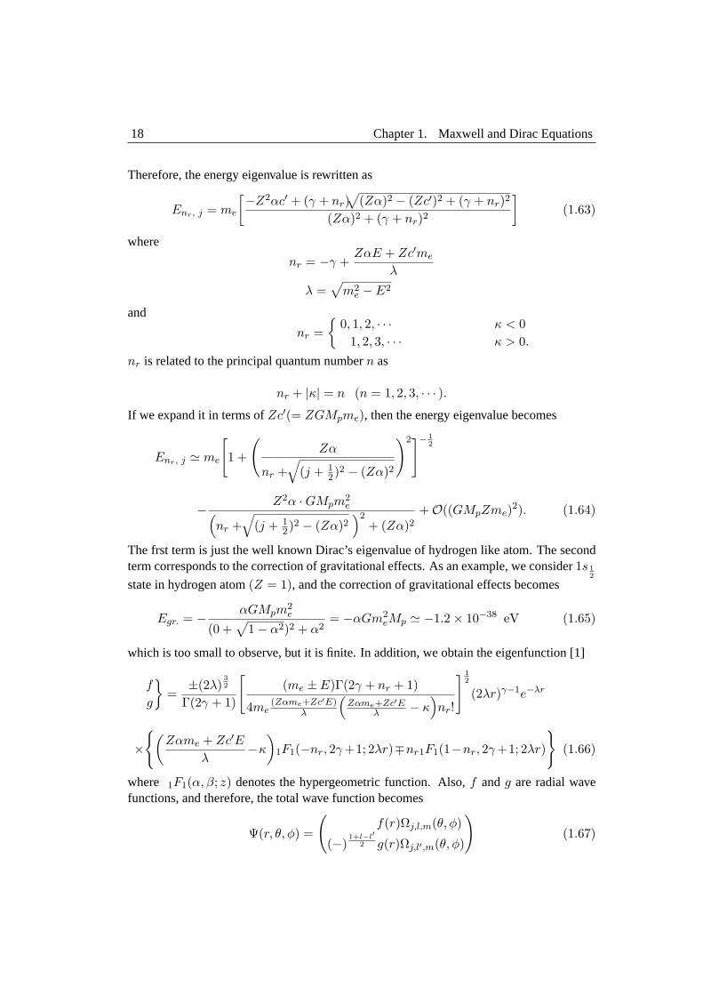
Therefore, the energy eigenvalue is rewritten as

Enr, j = me

[−Z2αc′ + (γ + nr)√

(Zα)2 − (Zc′)2 + (γ + nr)2

(Zα)2 + (γ + nr)2

](1.63)

where

nr = −γ +ZαE + Zc′me

λ

λ =√

m2e − E2

and

nr =

0, 1, 2, · · · κ < 01, 2, 3, · · · κ > 0.

nr is related to the principal quantum numbern as

nr + |κ| = n (n = 1, 2, 3, · · · ).If we expand it in terms ofZc′(= ZGMpme), then the energy eigenvalue becomes

Enr, j ' me

[1 +

(Zα

nr +√

(j + 12)2 − (Zα)2

)2]− 12

− Z2α ·GMpm2e(

nr +√

(j + 12)2 − (Zα)2

)2+ (Zα)2

+O((GMpZme)2). (1.64)

The frst term is just the well known Dirac’s eigenvalue of hydrogen like atom. The secondterm corresponds to the correction of gravitational effects. As an example, we consider1s 1

2

state in hydrogen atom(Z = 1), and the correction of gravitational effects becomes

Egr. = − αGMpm2e

(0 +√

1− α2)2 + α2= −αGm2

eMp ' −1.2× 10−38 eV (1.65)

which is too small to observe, but it is finite. In addition, we obtain the eigenfunction [1]

f

g

=

±(2λ)32

Γ(2γ + 1)

[(me ± E)Γ(2γ + nr + 1)

4me(Zαme+Zc′E)

λ

(Zαme+Zc′E

λ − κ)nr!

] 12

(2λr)γ−1e−λr

×(

Zαme + Zc′Eλ

−κ

)1F1(−nr, 2γ+1; 2λr)∓nr1F1(1−nr, 2γ+1; 2λr)

(1.66)

where 1F1(α, β; z) denotes the hypergeometric function. Also,f andg are radial wavefunctions, and therefore, the total wave function becomes

Ψ(r, θ, φ) =

(f(r)Ωj,l,m(θ, φ)

(−)1+l−l′

2 g(r)Ωj,l′,m(θ, φ)

)(1.67)


where

l = j ± 12

l′ = 2j − l

Ωj,l′,m(θ, φ) = il−l′(σ · r

r

)Ωj,l,m(θ, φ)

and

Ωl+ 12,l,m(θ, φ) =

√

j+m2j Y

m− 12

l (θ, φ)√j−m2j Y

m+ 12

l (θ, φ)

Ωl− 12,l,m(θ, φ) =

−

√j−m+12j+2 Y

m− 12

l (θ, φ)√j+m+12j+2 Y

m+ 12

l (θ, φ)

.

Classical Limits

As we see in the later chapter, the gravitational force becomes important when we discussthe motion of the planets in the Newton equation. When we make the non-relativisticreduction of the Dirac Hamiltonian, then we find

H =p2

2me− e2

r− GmeMp

r+

GMp

2merp2. (1.68)

Now, we make the classical limit of the Hamiltonian and obtain a new potential for theNewton equation with an additional gravitational potential

V (r) = −e2

r− GmeMp

r+

12mec2

(GmeMp

r

)2

. (1.69)

If the new potential is applied to the motion of the planets, then this additional gravitationalpotential turns out to be responsible for the description of the observed advance shifts ofthe Mercury perihelion, the GPS satellite motion and the earth rotation around the sun.

Conflict of InterestThe author(s) confirm that this article content has no conflicts interest.

Acknowledgements:Declared none.

Fundamental Problems in Quantum Field...

Documents

Transcript of Fundamental Problems in Quantum Field...