Fundamental Principles Governing Solvents...

2

Fundamental Principles

Governing Solvents Use

2.1 SOLVENT EFFECTS ON CHEMICAL SYSTEMS

Estanislao Silla, Arturo Arnau and Iñaki TuñóN

Department of Physical Chemistry, University of Valencia,Burjassot (Valencia), Spain

2.1.1 HISTORICAL OUTLINE

According to a story, a little fish asked a big fish about the ocean, since he had heard it beingtalked about but did not know where it was. Whilst the little fish’s eyes turned bright andshiny full of surprise, the old fish told him that all that surrounded him was the ocean. Thisstory illustrates in an eloquent way how difficult it is to get away from every day life, some-thing of which the chemistry of solvents is not unaware.

The chemistry of living beings and that which we practice in laboratories and factoriesis generally a chemistry in solution, a solution which is generally aqueous. A daily routinesuch as this explains the difficulty which, throughout the history of chemistry, has been en-countered in getting to know the effects of the solvent in chemical transformations, some-thing which was not achieved in a precise way until well into the XX century. It wasnecessary to wait for the development of experimental techniques in vacuo to be able to sep-arate the solvent and to compare the chemical processes in the presence and in the absenceof this, with the purpose of getting to know its role in the chemical transformations whichoccur in its midst. But we ought to start from the beginning.

Although essential for the later cultural development, Greek philosophy was basicallya work of the imagination, removed from experimentation, and something more than medi-tation is needed to reach an approach on what happens in a process of dissolution. However,in those remote times, any chemically active liquid was included under the name of “divinewater”, bearing in mind that the term “water” was used to refer to anything liquid or dis-solved.1

Parallel with the fanciful search for the philosopher’s stone, the alchemists toiledaway on another impossible search, that of a universal solvent which some called “alkahest”and others referred to as “menstruum universale”, which term was used by the veryParacelsus (1493-1541), which gives an idea of the importance given to solvents during thatdark and obscurantist period. Even though the “menstruum universale” proved just as elu-sive as the philosopher’s stone, all the work carried out by the alchemists in search of these

illusionary materials opened the way to improving the work in the laboratory, the develop-ment of new methods, the discovery of compounds and the utilization of novel solvents.One of the tangible results of all that alchemistry work was the discovery of one of the firstexperimental rules of chemistry: “similia similibus solvuntor”, which reminds us of thecompatibility in solution of those substances of similar nature.

Even so, the alchemistry only touched lightly on the subject of the role played by thesolvent, with so many conceptual gulfs in those pre-scientific times in which the terms dis-solution and solution referred to any process which led to a liquid product, without makingany distinction between the fusion of a substance - such as the transformation of ice into liq-uid water -, mere physical dissolution - such as that of a sweetener in water - or the dissolu-tion which takes place with a chemical transformation - such as could be the dissolution of ametal in an acid. This misdirected vision of the dissolution process led the alchemists downequally erroneous collateral paths which were prolonged in time. Some examples are worthquoting: Hermann Boerhaave (1688-1738) thought that dissolution and chemical reactionconstituted the same reality; the solvent, (menstruum), habitually a liquid, he considered tobe formed by diminutive particles moving around amongst those of the solute, leaving theinteractions of these particles dependent on the mutual affinities of both substances.2 Thispaved the way for Boerhaave to introduce the term affinity in a such a way as was conservedthroughout the whole of the following century.3 This approach also enabled Boerhaave toconclude that combustion was accompanied by an increase of weight due to the capturing of“particles” of fire, which he considered to be provided with weight by the substance whichwas burned. This explanation, supported by the well known Boyle, eased the way to consid-ering that fire, heat and light were material substances until when, in the XIX century, themodern concept of energy put things in their place.4

Even Bertollet (1748-1822) saw no difference between a dissolution and a chemicalreaction, which prevented him from reaching the law of definite proportions. It was Proust,an experimenter who was more exacting and capable of differentiating between chemicalreaction and dissolution, who made his opinion prevail:

“The dissolution of ammonia in water is not the same as that ofhydrogen in azote (nitrogen), which gives rise to ammonia”5

There were also alchemists who defended the idea that the substances lost their naturewhen dissolved. Van Helmont (1577-1644) was one of the first to oppose this mistaken ideaby defending that the substance dissolved remains in the solution in aqueous form, it beingpossible to recover it later. Later, the theories of osmotic pressure of van´t Hoff (1852-1911)and that of electrolytic dissociation of Arrhenius (1859-1927) took this approach even fur-ther.

Until almost the end of the XIX century the effects of the solvent on the differentchemical processes did not become the object of systematic study by the experimenters. Theeffect of the solvent was assumed, without reaching the point of awakening the interest ofthe chemists. However, some chemists of the XIX century were soon capable of unravelingthe role played by some solvents by carrying out experiments on different solvents, classi-fied according to their physical properties; in this way the influence of the solvent both onchemical equilibrium and on the rate of reaction was brought to light. Thus, in 1862,Berthelot and Saint-Gilles, in their studies on the esterification of acetic acid with ethanol,

8 Estanislao Silla, Arturo Arnau and Iñaki Tuñón

discovered that some solvents, which do not participate in the chemical reaction, are capa-ble of slowing down the process.6 In 1890, Menschutkin, in a now classical study on the re-action of the trialkylamines with haloalcans in 23 solvents, made it clear how the choice ofone or the other could substantially affect the reaction rate.7 It was also Menschutkin whodiscovered that, in reactions between liquids, one of the reactants could constitute a solventinadvisable for that reaction. Thus, in the reaction between aniline and acetic acid to pro-duce acetanilide, it is better to use an excess of acetic acid than an excess of aniline, since thelatter is a solvent which is not very favorable to this reaction.

The fruits of these experiments with series of solvents were the first rules regarding theparticipation of the solvent, such as those discovered by Hughes and Ingold for the rate ofthe nucleophilic reactions.8 Utilizing a simple electrostatic model of the solute - solvent in-teractions, Hughes and Ingold concluded that the state of transition is more polar than theinitial state, that an increase of the polarity of the solvent will stabilize the state of transitionwith respect to the initial state, thus leading to an increase in the reaction rate. If, on the con-trary, the state of transition is less polar, then the increase of the polarity of the solvent willlead to a decrease of the velocity of the process. The rules of Hughes-Ingold for thenucleophilic aliphatic reactions are summarized in Table 2.1.1.

Table 2.1.1. Rules of Hughes-Ingold on the effect of the increase of the polarity of thesolvent on the rate of nucleophilic aliphatic reactions

Mechanism Initial state State of transition Effect on the reaction rate

SN2

Y- + RX [Y--R--X]- slight decrease

Y + RX [Y--R--X] large increase

Y- + RX+ [Y--R--X] large decrease

Y + RX+ [Y--R--X]+ slight decrease

SN1RX [R--X] large increase

RX+ [R--X]+ slight decrease

In 1896 the first results about the role of the solvent on chemical equilibria were ob-tained, coinciding with the discovery of the keto-enolic tautomerism.9 Claisen identified themedium as one of the factors which, together with the temperature and the substituents,proved to be decisive in this equilibrium. Soon systematic studies began to be done on theeffect of the solvent in the tautomeric equilibria. Wislicenus studied the keto-enolic equilib-rium of ethylformylphenylacetate in eight solvents, concluding that the final proportion be-tween the keto form and the enol form depended on the polarity of the solvent.10 This effectof the solvent also revealed itself in other types of equilibria: acid-base, conformational,those of isomerization and of electronic transfer. The acid-base equilibrium is of particularinterest. The relative scales of basicity and acidity of different organic compounds and ho-mologous families were established on the basis of measurements carried out in solution,fundamentally aqueous. These scales permitted establishing hypotheses regarding the ef-fect of the substituents on the acidic and basic centers, but without being capable of separat-ing this from the effect of the solvent. Thus, the scale obtained in solution for the acidity of

2.1 Solvent effects on chemical systems 9

the α-substituted methyl alcohols [(CH3)3COH > (CH3)2CHOH > CH3CH2OH > CH3OH]11

came into conflict with the conclusions extracted from the measurements of movements byNMR.12 The irregular order in the basicity of the methyl amines in aqueous solution alsoproved to be confusing [NH3 < CH3NH2 < (CH3)2NH > (CH3)3N],13 since it did not matchany of the existing models on the effects of the substituents. These conflicts were only re-solved when the scales of acidity-basicity were established in the gas phase. On carrying outthe abstraction of the solvent an exact understanding began to be had of the real role itplayed.

The great technological development which arrived with the XIX century has broughtus a set of techniques capable of giving accurate values in the study of chemical processes inthe gas phase. The methods most widely used for these studies are:

• The High Pressure Mass Spectrometry, which uses a beam of electron pulses14

• The Ion Cyclotron Resonance and its corresponding Fourier Transform (FT-ICR)15

• The Chemical Ionization Mass Spectrometry, in which the analysis is made of thekinetic energy of the ions, after generating them by collisions16

• The techniques of Flowing Afterglow, where the flow of gases is submitted toionization by electron bombardment17-19

All of these techniques give absolute values with an accuracy of ±(2-4) Kcal/mol andof ±0.2 Kcal/mol for the relative values.20

During the last decades of XX century the importance has also been made clear of theeffects of the solvent in the behavior of the biomacromolecules. To give an example, the in-fluence of the solvent over the proteins is made evident not only by its effects on the struc-ture and the thermodynamics, but also on the dynamics of these, both at local as well as atglobal level.21 In the same way, the effect of the medium proves to be indispensable in ex-plaining a large variety of biological processes, such us the rate of interchange of oxygen inmyoglobin.22 Therefore, the actual state of development of chemistry, as much in its experi-mental aspect as in its theoretical one, allows us to identify and analyze the influence of thesolvent on processes increasingly more complex, leaving the subject open for new chal-lenges and investigating the scientific necessity of creating models with which to interpretsuch a wide range of phenomena as this. The little fish became aware of the ocean and beganexplorations.

2.1.2 CLASSIFICATION OF SOLUTE-SOLVENT INTERACTIONS

Fixing the limits of the different interactions between the solute and the solvent which enve-lopes it is not a trivial task. In the first place, the liquid state, which is predominant in themajority of the solutions in use, is more difficult to comprehend than the solid state (whichhas its constitutive particles, atoms, molecules or ions, in fixed positions) or the gaseousstate (in which the interactions between the constitutive particles are not so intense). More-over, the solute-solvent interactions, which, as has already been pointed out, generally hap-pen in the liquid phase, are half way between the predominant interactions in the solid phaseand those which happen in the gas phase, too weak to be likened with the physics of the solidstate but too strong to fit in with the kinetic theory of gases. In the second place, dissectingthe solute-solvent interaction into different sub-interactions only serves to give us an ap-proximate idea of the reality and we should not forget that, in the solute-solvent interaction,the all is not the sum of the parts. In the third place, the world of the solvents is very variedfrom those which have a very severe internal structure, as in the case of water, to those


whose molecules interact superficially, as in the case of the hydrocarbons. At all events,there is no alternative to meeting the challenge face to face.

If we mix a solute and a solvent, both being constituted by chemically saturated mole-cules, their molecules attract one another as they approach one another. This interaction canonly be electrical in its nature, given that other known interactions are much more intenseand of much shorter range of action (such as those which can be explained by means of nu-clear forces) or much lighter and of longer range of action (such as the gravitational force).These intermolecular forces usually also receive the name of van der Waals forces, from thefact that it was this Dutch physicist, Johannes D. van der Waals (1837-1923), who recog-nized them as being the cause of the non-perfect behavior of the real gases, in a period inwhich the modern concept of the molecule still had to be consolidated. The intermolecularforces not only permit the interactions between solutes and solvents to be explained but alsodetermine the properties of gases, liquids and solids; they are essential in the chemical trans-formations and are responsible for organizing the structure of biological molecules.

The analysis of solute-solvent interactions is usually based on the following partitionscheme:

∆ ∆ ∆ ∆E E E Ei ij jj= + + [2.1.1]

where i stands for the solute and j for the solvent.This approach can be maintained while theidentities of the solute and solvent molecules are preserved. In some special cases (see be-low in specific interactions) it will be necessary to include some solvent molecules in thesolute definition.

The first term in the above expression is the energy change of the solute due to theelectronic and nuclear distortion induced by the solvent molecule and is usually given thename solute polarization. ∆Eij is the interaction energy between the solute and solvent mole-cules. The last term is the energy difference between the solvent after and before the intro-duction of the solute. This term reflects the changes induced by the solute on the solventstructure. It is usually called cavitation energy in the framework of continuum solvent mod-els and hydrophobic interaction when analyzing the solvation of nonpolar molecules.

The calculation of the three energy terms needs analytical expressions for the differentenergy contributions but also requires knowledge of solvent molecules distribution aroundthe solute which in turn depends on the balance between the potential and the kinetic energyof the molecules. This distribution can be obtained from diffraction experiments or moreusually is calculated by means of different solvent modelling. In this section we will com-ment on the expression for evaluating the energy contributions. The first two terms in equa-tion [2.1.1] can be considered together by means of the following energy partition :

∆ ∆ ∆ ∆ ∆E E E E Ei ij el pol d r+ = + + − [2.1.2]

Analytical expressions for the three terms (electrostatic, polarization and disper-sion-repulsion energies) are obtained from the intermolecular interactions theory.

2.1.2.1 Electrostatic

The electrostatic contribution arises from the interaction of the unpolarized charge distribu-tion of the molecules. This interaction can be analyzed using a multipolar expansion of thecharge distribution of the interacting subsystems which usually is cut off in the first term


which is different from zero. If both the solute and the solvent are considered to be formedby neutral polar molecules (with a permanent dipolar moment different from zero), due toan asymmetric distribution of its charges, the electric interaction of the type dipole-dipolewill normally be the most important term in the electrostatic interaction. The intensity ofthis interaction will depend on the relative orientation of the dipoles. If the molecular rota-tion is not restricted, we must consider the weighted average over different orientations

EkTr

d d− = −2

3 6

µ µ(4πε)

12

22

2[2.1.3]

where:µ i, µ j dipole momentsk Boltzmann constantε dielectric constantT absolute temperaturer intermolecular distance

The most stable orientation is the antiparallel, except in the case that the molecules inplay are very voluminous. Two dipoles inrapid thermal movement will be orientatedsometimes in a way such that they are at-tracted and at other times in a way that theyare repelled. On the average, the net energyturns out to be attractive. It also has to beborne in mind that the thermal energy of themolecules is a serious obstacle for the di-poles to be oriented in an optimum manner.The average potential energy of the di-pole-dipole interaction, or of orientation, is,therefore, very dependent on the tempera-ture.

In the event that one of the species in-volved were not neutral (for example an an-

ionic or cationic solute) the predominant term in the series which gives the electrostaticinteraction will be the ion-dipole which is given by the expression:

Eq

kTri d

i j

− = −2 2

2 46 4

µ

πε( )[2.1.4]

2.1.2.2 Polarization

If we dissolve a polar substance in a nonpolar solvent, the molecular dipoles of the solute arecapable of distorting the electronic clouds of the solvent molecules inducing the appearancein these of new dipoles. The dipoles of solute and those induced will line up and will be at-tracted and the energy of this interaction (also called interaction of polarization or induc-tion) is:


Figure 2.1.1. The dipoles of two molecules can approachone another under an infinite variety of attractive orienta-tions, among which these two extreme orientations standout.

Er

d id

j i

− = −α µ

πε

2

2 64( )[2.1.5]

where:µ i dipole momentα j polarizabilityr intermolecular distance

In a similar way, the dissolution of an ionic substance in a nonpolar solvent also willoccur with the induction of the dipoles in the molecules of the solvent by the solute ions.

These equations make reference to the interactions between two molecules. Becausethe polarization energy (of the solute or of the solvent) is not pairwise additive magnitude,the consideration of a third molecule should be carried out simultaneously, it being impossi-ble to decompose the interaction of the three bodies in a sum of the interactions of two bod-ies. The interactions between molecules in solution are different from those which takeplace between isolated molecules. For this reason, the dipolar moment of a molecule mayvary considerably from the gas phase to the solution, and will depend in a complicated fash-ion on the interactions which may take place between the molecule of solute and its specificsurroundings of molecules of solvent.

2.1.2.3 Dispersion

Even when solvent and solute are constituted by nonpolar molecules, there is interaction be-tween them. It was F. London who was first to face up to this problem, for which reasonthese forces are known as London’s forces, but also as dispersion forces, charge-fluctua-tions forces or electrodynamic forces. Their origin is as follows: when we say that a sub-stance is nonpolar we are indicating that the distribution of the charges of its molecules issymmetrical throughout a wide average time span. But, without doubt, in an interval of timesufficiently restricted the molecular movements generate displacements of their chargeswhich break that symmetry giving birth to instantaneous dipoles. Since the orientation ofthe dipolar moment vector is varying constantly due to the molecular movement, the aver-age dipolar moment is zero, which does not prevent the existence of these interactions be-tween momentary dipoles. Starting with two instantaneous dipoles, these will be oriented toreach a disposition which will favor them energetically. The energy of this dispersion inter-action can be given, to a first approximation, by:

EI I

I I rdisp

i j

i j

i j= −+

3

2 4 2 6( ) ( )πε

α α[2.1.6]

where:Ii, Ij ionization potentialsα i, α j polarizabilitiesr intermolecular distance

From equation [2.1.6] it becomes evident that dispersion is an interaction which ismore noticeable the greater the volume of molecules involved. The dispersion forces are of-ten more intense than the electrostatic forces and, in any case, are universal for all the atomsand molecules, given that they are not seen to be subjected to the requirement that perma-nent dipoles should exist beforehand. These forces are responsible for the aggregation ofthe substances which possess neither free charges nor permanent dipoles, and are also the


protagonists of phenomena such as surface tension, adhesion, flocculation, physical adsorp-tion, etc. Although the origin of the dispersion forces may be understood intuitively, this isof a quantum mechanical nature.

2.1.2.4 Repulsion

Between two molecules where attractive forces are acting, which could cause them to be su-perimposed, it is evident that also repulsive forces exist which determine the distance towhich the molecules (or the atoms) approach one another. These repulsive forces are a con-sequence of the overlapping of the electronic molecular clouds when these are nearing oneanother. These are also known as steric repulsion, hard core repulsion or exchange repul-sion. They are forces of short range which grow rapidly when the molecules which interactapproach one another, and which enter within the ambit of quantum mechanics. Throughoutthe years, different empirical potentials have been obtained with which the effect of theseforces can be reproduced. In the model hard sphere potential, the molecules are supposed tobe rigid spheres, such that the repulsive force becomes suddenly infinite, after a certain dis-tance during the approach. Mathematically this potential is:

Er

rep =

∞σ[2.1.7]

where:r intermolecular distanceσ hard sphere diameter

Other repulsion potentials are the power-law potential:

Er

rep

n

=

σ[2.1.8]

where:r intermolecular distancen integer, usually between 9 and 16σ sphere diameter

and the exponential potential:

E Cr

rep = −

exp

σ0

[2.1.9]

where:r intermolecular distanceC adjustable constantσo adjustable constant

These last two potentials allow a certain compressibility of the molecules, more inconsonance with reality, and for this reason they are also known as soft repulsion.

If we represent the repulsion energy by a term proportional to r-12, and given that theenergy of attraction between molecules decreases in proportion to r-6 at distances above themolecular diameter, we can obtain the total potential of interaction:

E Ar Br= − +− −6 12 [2.1.10]


where:r intermolecular distanceA constantB constant

which receives the name of potential “6-12”or potential of Lennard-Jones,23 widely usedfor its mathematical simplicity (Figure2.1.3)

2.1.2.5 Specific interactions

Water, the most common liquid, the “uni-versal solvent”, is just a little “extraordi-nary”, and this exceptional nature of the“liquid element” is essential for the worldwhich has harbored us to keep on doing so.It is not normal that a substance in its solidstate should be less dense than in the liquid,but if one ill-fated day a piece of ice sponta-neously stopped floating on liquid water, allwould be lost, the huge mass of ice which isfloating in the colder seas could sink thusraising the level of water in the oceans.

For a liquid with such a small molecu-lar mass, water has melting and boiling tem-peratures and a latent heat of vaporizationwhich are unexpectedly high. Also unusualare its low compressibility, its high dipolarmoment, its high dielectric constant and thefact that its density is maximum at 4 ºC. Allthis proves that water is an extraordinarilycomplex liquid in which the intermolecularforces exhibit specific interactions, theso-called hydrogen bonds, about which it isnecessary to know more.

Hydrogen bonds appear in substanceswhere there is hydrogen united covalently to

very electronegative elements (e.g., F, Cl, O and N), which is the case with water. The hy-drogen bond can be either intermolecular (e.g., H2O) or intramolecular (e.g., DNA). Theprotagonism of hydrogen is due to its small size and its tendency to become positively po-larized, specifically to the elevated density of the charge which accumulates on the men-tioned compounds. In this way, hydrogen is capable, such as in the case of water, of beingdoubly bonded: on the one hand it is united covalently to an atom of oxygen belonging to itsmolecule and, on the other, it electrostatically attracts another atom of oxygen belonging toanother molecule, so strengthening the attractions between molecules. In this way, eachatom of oxygen of a molecule of water can take part in four links with four more moleculesof water, two of these links being through the hydrogen atoms covalently united to it and theother two links through hydrogen bonds thanks to the two pairs of solitary electrons which it


Figure 2.1.2. Hard-sphere repulsion (a) and soft repul-sion (b) between two atoms.

Figure 2.1.3. Lennard-Jones potential between two at-oms.

possesses. The presence of the hydrogenbonds together with this tetrahedric coordi-nation of the molecule of water constitutethe key to explaining its unusual properties.

The energy of this bond (10-40KJ/mol) is found to be between that corre-sponding to the van der Waals forces (~1KJ/mol) and that corresponding to the sim-ple covalent bond (200-400 KJ/mol). Anenergetic analysis of the hydrogen bond in-teraction shows that the leading term is theelectrostatic one which explains that stronghydrogen bonds are found between hydro-gen atoms with a partial positive charge anda basic site. The second term in the energydecomposition of the hydrogen bond inter-action is the charge transfer.24

The hydrogen bonds are crucial in ex-plaining the form of the large biological molecules, such as the proteins and the nucleic ac-ids, as well as how to begin to understand more particular chemical phenomena.25

Those solutes which are capable of forming hydrogen bonds have a well known affin-ity for the solvents with a similar characteristic, which is the case of water. The formation ofhydrogen bonds between solute molecules and those of the solvent explains, for example,the good solubility in water of ammonia and of the short chain organic acids.

2.1.2.6 Hydrophobic interactions

On the other hand, those nonpolar solutes which are not capable of forming hydrogen bondswith water, such as the case of the hydrocarbons, interact with it in a particular way. Let usimagine a molecule of solute incapable of forming hydrogen bonds in the midst of the water.Those molecules of water which come close to that molecule of solute will lose some or allof the hydrogen bonds which they were sharing with the other molecules of water. Thisobliges the molecules of water which surround those of solute to arrange themselves inspace so that there is a loss of the least number of hydrogen bonds with other molecules ofwater. Evidently, this rearrangement (solvation or hydration) of the water molecules aroundthe nonpolar molecule of solute will be greatly conditioned by the form and the size of thislatter. All this amounts to a low solubility of nonpolar substances in water, which is knownas the hydrophobic effect. If we now imagine not one but two nonpolar molecules in themidst of the water, it emerges that the interaction between these two molecules is greaterwhen they are interacting in a free space. This phenomenon, also related to the rearrange-ment of the molecules of water around those of the solute, receives the name of hydrophobicinteraction.

The hydrophobic interaction term is used to describe the tendency of non-polar groupsor molecules to aggregate in water solution.26 Hydrophobic interactions are believed to playa very important role in a variety of processes, specially in the behavior of proteins in aque-ous media. The origin of this solvent-induced interactions is still unclear. In 1945 Frank andEvans27 proposed the so-called iceberg model where emphasis is made on the enhanced lo-cal structure of water around the non-polar solute. However, computational studies and ex-


Figure 2.1.4. Tetrahedric structure of water in a crystal ofice. The dotted lines indicate the hydrogen bridges.

perimental advances have yielded increasing evidence against the traditionalinterpretation,28 and other alternative explanations, such as the reduced freedom of watermolecules in the solvation shell,29 have emerged.

To understand the hydrophobic interaction at the microscopic level molecular simula-tions of non-polar compounds in water have been carried out.30 The potential of mean forcebetween two non-polar molecules shows a contact minimum with an energy barrier. Com-puter simulations also usually predict the existence of a second solvent-separated mini-mum. Although molecular simulations provide valuable microscopic information onhydrophobic interactions they are computationally very expensive, specially for large sys-tems, and normally make use of oversimplified potentials. The hydrophobic interaction canalso be alternatively studied by means of continuum models.31 Using this approach a differ-ent but complementary view of the problem has been obtained. In the partition energyscheme used in the continuum models (see below and Chapter 8) the cavitation free energy(due to the change in the solvent-solvent interactions) is the most important contribution tothe potential of mean force between two non-polar solutes in aqueous solution, being re-sponsible for the energy barrier that separates the contact minimum. The electrostatic con-tribution to the potential of mean force for two non-polar molecules in water is close to zeroand the dispersion-repulsion term remains approximately constant. The cavitation free en-ergy only depends on the surface of the cavity where the solute is embedded and on the sol-vent physical properties (such as the surface tension and density).

2.1.3 MODELLING OF SOLVENT EFFECTS

A useful way of understanding the interaction between the molecules of solvent and those ofsolute can be done by reproducing it by means of an adequate model. This task of imitationof the dissolution process usually goes beyond the use of simple and intuitive structuralmodels, such as “stick” models, which prove to be very useful both in labors of teaching asin those of research, and frequently require the performance of a very high number of com-plex mathematical operations.

Even though, in the first instance, we could think that a solution could be considered asa group of molecules united by relatively weak interactions, the reality is more complex, es-pecially if we analyze the chemical reactivity in the midst of a solvent. The prediction of re-action mechanisms, the calculation of reaction rates, the obtaining of the structures ofminimum energy and other precise aspects of the chemical processes in solution require thesupport of models with a very elaborated formalism and also of powerful computers.

Traditionally, the models which permit the reproduction of the solute-solvent interac-tions are classified into three groups:32

i Those based on the simulation of liquids by means of computers.ii Those of continuum.iii Those of the supermolecule type.In the models classifiable into the first group, the system analyzed is represented by

means of a group of interacting particles and the statistical distribution of any property iscalculated as the the average over the different configurations generated in the simulation.Especially notable among these models are those of Molecular Dynamics and those of theMonte Carlo type.

The continuum models center their attention on a microscopic description of the solutemolecules, whilst the solvent is globally represented by means of its macroscopic proper-ties, such as its density, its refractive index, or its dielectric constant.


Finally, the supermolecule type models restrict the analysis to the interaction amongjust a few molecules described at a quantum level which leads to a rigorous treatment oftheir interactions but does not allow us to have exact information about the global effect ofthe solvent on the solute molecules, which usually is a very long range effect.

The majority of these models have their origin in a physical analysis of the solutionsbut, with the passage of time, they have acquired a more chemical connotation, they havecentered the analysis more on the molecular aspect. As well as this, recourse is more andmore being made to combined strategies which use the best of each of the methods referredto in pursuit of a truer reproduction of the solute-disolvente interactions. Specially usefulhas been shown to be a combination of the supermolecular method, used to reproduce thespecific interactions between the solute and one or two molecules of the solvent, with thoseof continuum or of simulation, used to reproduce the global properties of the medium.

2.1.3.1 Computer simulations

Obtaining the configuration or the conformation of minimum energy of a system providesus with a static view of this which may be sufficient to obtain many of its properties. How-ever, direct comparison with experiments can be strictly be done only if average thermody-namic properties are obtained. Simulation methods are designed to calculate averageproperties of a system over many different configurations which are generated for beingrepresentative of the system behavior. These methods are based in the calculation of aver-age properties as a sum over discrete events:

F dR dR P R F R P Fn i i

i

N

= ≈=∑∫ 1

1

K ( ) ( ) [2.1.11]

Two important difficulties arise in the computation of an average property as a sum.First, the number of molecules that can be handled in a computer is of the order of a fewhundred. Secondly, the number of configurations needed to reach the convergency in thesum can be too great. The first problem can be solved by different computational strategies,such as the imposition of periodic boundary conditions.33 The solution of the second prob-lem differs among the main used techniques in computer simulations.

The two techniques most used in the dynamic study of the molecular systems are theMolecular Dynamics, whose origin dates back34 to 1957, and the Monte Carlo methods,which came into being following the first simulation of fluids by computer,35 which oc-curred in 1952.

Molecular DynamicsIn the Molecular Dynamic simulations, generation of new system configurations or se-quence of events is made following the trajectory of the system which is dictated by theequations of motion. Thus, this methods leads to the computation of time averages and per-mits the calculation of not only equilibrium but also transport properties. Given a configura-tion of the system, a new configuration is obtained moving the molecules according to thetotal force exerted on them:

md R

dtE R

j

j jk

k

n2

21

= − ∇=

∑ ( ) [2.1.12]


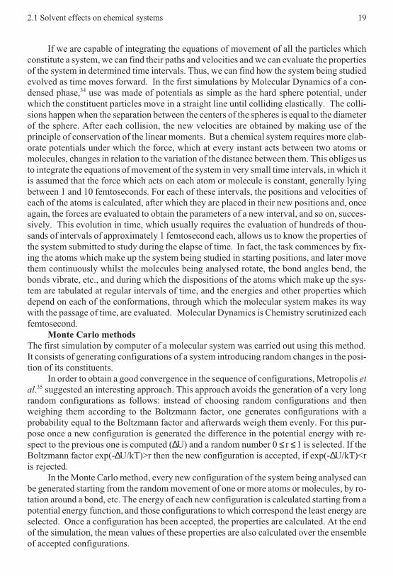
If we are capable of integrating the equations of movement of all the particles whichconstitute a system, we can find their paths and velocities and we can evaluate the propertiesof the system in determined time intervals. Thus, we can find how the system being studiedevolved as time moves forward. In the first simulations by Molecular Dynamics of a con-densed phase,34 use was made of potentials as simple as the hard sphere potential, underwhich the constituent particles move in a straight line until colliding elastically. The colli-sions happen when the separation between the centers of the spheres is equal to the diameterof the sphere. After each collision, the new velocities are obtained by making use of theprinciple of conservation of the linear moments. But a chemical system requires more elab-orate potentials under which the force, which at every instant acts between two atoms ormolecules, changes in relation to the variation of the distance between them. This obliges usto integrate the equations of movement of the system in very small time intervals, in which itis assumed that the force which acts on each atom or molecule is constant, generally lyingbetween 1 and 10 femtoseconds. For each of these intervals, the positions and velocities ofeach of the atoms is calculated, after which they are placed in their new positions and, onceagain, the forces are evaluated to obtain the parameters of a new interval, and so on, succes-sively. This evolution in time, which usually requires the evaluation of hundreds of thou-sands of intervals of approximately 1 femtosecond each, allows us to know the properties ofthe system submitted to study during the elapse of time. In fact, the task commences by fix-ing the atoms which make up the system being studied in starting positions, and later movethem continuously whilst the molecules being analysed rotate, the bond angles bend, thebonds vibrate, etc., and during which the dispositions of the atoms which make up the sys-tem are tabulated at regular intervals of time, and the energies and other properties whichdepend on each of the conformations, through which the molecular system makes its waywith the passage of time, are evaluated. Molecular Dynamics is Chemistry scrutinized eachfemtosecond.

Monte Carlo methodsThe first simulation by computer of a molecular system was carried out using this method.It consists of generating configurations of a system introducing random changes in the posi-tion of its constituents.

In order to obtain a good convergence in the sequence of configurations, Metropolis etal.35 suggested an interesting approach. This approach avoids the generation of a very longrandom configurations as follows: instead of choosing random configurations and thenweighing them according to the Boltzmann factor, one generates configurations with aprobability equal to the Boltzmann factor and afterwards weigh them evenly. For this pur-pose once a new configuration is generated the difference in the potential energy with re-spect to the previous one is computed (∆U) and a random number 0 ≤ r ≤1 is selected. If theBoltzmann factor exp(-∆U/kT)>r then the new configuration is accepted, if exp(-∆U/kT)<ris rejected.

In the Monte Carlo method, every new configuration of the system being analysed canbe generated starting from the random movement of one or more atoms or molecules, by ro-tation around a bond, etc. The energy of each new configuration is calculated starting from apotential energy function, and those configurations to which correspond the least energy areselected. Once a configuration has been accepted, the properties are calculated. At the endof the simulation, the mean values of these properties are also calculated over the ensembleof accepted configurations.


When the moment comes to face the task of modelling a dissolution process, certaindoubts may arise about the convenience of using Molecular Dynamics or a Monte Carlomethod. It must be accepted that a simulation with Molecular Dynamics is a succession ofconfigurations which are linked together in time, in a similar way that a film is a collectionof scenes which follow one after the other. When one of the configurations of the systemanalysed by Molecular Dynamics has been obtained, it is not possible to relate it to thosewhich precede it or those which follow, which is something which does not occur in theMonte Carlo type of simulations. In these, the configurations are generated in a randomway, without fixed timing, and each configuration is only related to that which immediatelypreceded it. It would therefore seem advisable to make use of Molecular Dynamics to studya system through a period of time. On the other hand, the Monte Carlo method is usually themost appropriate when we are able to do without the requirement of time. Even so, it is ad-visable to combine adequately the two techniques in the different parts of the simulation, us-ing a hybrid arrangement. In this way, the evolution of the process of the dissolution of amacromolecule can be followed by Molecular Dynamics and make use of the Monte Carlomethod to resolve some of the steps of the overall process. On the other hand, its is fre-quently made a distinction in the electronic description of solute and solvent. So, as thechemical attention is focused on the solute, a quantum treatment is used for it while the restof the system is described at the molecular mechanics level.36

2.1.3.2 Continuum models

In many dissolution processes the solvent merely acts to provide an enveloping surround-ing for the solute molecules, the specific interactions with the solvent molecules are not ofnote but the dielectric of the solvent does significantly affect the solute molecules. This sortof situation can be confronted considering the solvent as a continuum, without including ex-plicitly each of its molecules and concentrating on the behavior of the solute. A large num-ber of models have been designed with this approach, either using quantum mechanics orresorting to empirical models. They are the continuum models.32 The continuum modelshave attached to their relative simplicity, and therefore a lesser degree of computational cal-culation, a favorable description of many chemical problems in dissolution, from the pointof view of the chemical equilibrium, kinetics, thermochemistry, spectroscopy, etc.

Generally, the analysis of a chemical problem with a model of continuum begins bydefining a cavity - in which a molecule of solute will be inserted - in the midst of the dielec-tric medium which represents the solvent. Differently to the simulation methods, where thesolvent distribution function is obtained during the calculation, in the continuum modelsthis distribution is usually assumed to be constant outside of the solute cavity and its value istaken to reproduce the macroscopic density of the solvent.

Although the continuum models were initially created with the aim of the calculationof the electrostatic contribution to the solvation free energy,37 they have been nowadays ex-tended for the consideration of other energy contributions. So, the solvation free energy isusually expressed in these models as the sum of three different terms:

∆ ∆ ∆ ∆G G G Gsol ele dis rep cav= + +− [2.1.13]

where the first term is the electrostatic contribution, the second one the sum of dispersionand repulsion energies and the third one the energy needed to create the solute cavity in thesolvent. Specific interactions can be also added if necessary.


For the calculation of the electrostatic term the system under study is characterized bytwo dielectric constants, in the interior of the cavity the constant will have a value of unity,and in the exterior the value of the dielectric constant of the solvent. From this point the to-tal electrostatic potential is evaluated. Beyond the mere classical outlining of the problem,Quantum Mechanics allows us to examine more deeply the analysis of the solute inserted inthe field of reaction of the solvent, making the relevant modifications in the quantum me-chanical equations of the system under study with a view to introducing a term due to thesolvent reaction field.38 This permits a widening of the benefits which the use of the contin-uum methods grant to other facilities provided for a quantical treatment of the system, suchas the optimization of the solute geometry,39 the analysis of its wave function,40 the obtain-ing of its harmonic frequencies,41 etc.; all of which in the presence of the solvent. In thisway a full analysis of the interaction solute-solvent can be reached at low computationalcost.

Continuum models essentially differ in:• How the solute is described, either classically

or quantally• How the solute charge distribution and its

interaction with the dielectric are obtained• How the solute cavity and its surface are

described.The first two topics are thoroughly consid-

ered in Chapter 8 by Prof. Tomasi, here we willconsider in detail the last topic.

2.1.3.3. Cavity surfaces

Earliest continuum models made use of oversim-plified cavities for the insertion of the solute in thedielectric medium such as spheres or ellipsoids. Inthe last decades, the concept of molecular surfaceas become more common. Thus, the surface hasbeen used in microscopic models of solution.38,42

Linear relationships were also found between mo-lecular surfaces and solvation free energies.43

Moreover, given that molecular surfaces can helpus in the calculation of the interaction of a solutemolecule with surroundings of solvent molecules,they are one of the main tools in understanding thesolution processes and solvent effects on chemicalsystems. Another popular application is the gener-ation of graphic displays.44

One may use different types of molecularcavities and surfaces definitions (e.g.equipotential surfaces, equidensity surfaces, vander Waals surfaces). Among them there is a subsetthat shares a common trait: they consider that amolecule may be represented as a set of rigid inter-locking spheres. There are three such surfaces: a)


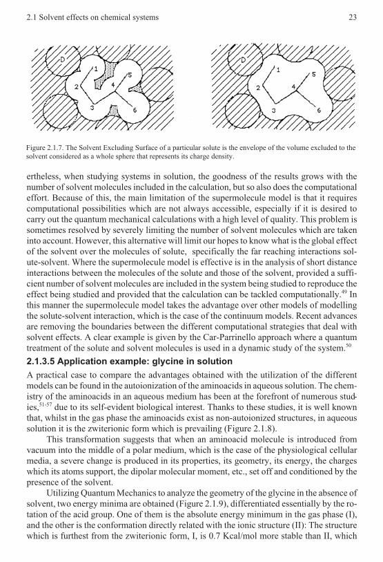
Figure 2.1.5. Molecular Surface models. (a) vander Waals Surface; (b) Accessible Surface and(c) Solvent Excluding Surface.

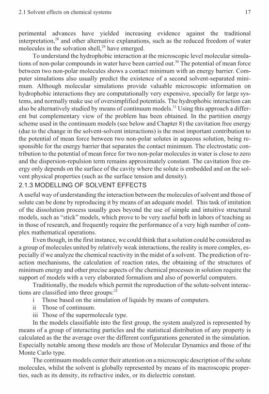
the van der Waals surface (WSURF), which is the external surface resulting from a set ofspheres centered on the atoms or group of atoms forming the molecule (Figure 2.1.5a); b)the Accessible Surface (ASURF), defined by Richards and Lee45 as the surface generated bythe center of the solvent probe sphere, when it rolls around the van der Waals surface (Fig-ure 2.1.5b); and c) the Solvent Excluding Surface (ESURF) which was defined byRichards46 as the molecular surface and defined by him as composed of two parts: the con-tact surface and the reentrant surface. The contact surface is the part of the van der Waalssurface of each atom which is accessible to a probe sphere of a given radius. The reentrantsurface is defined as the inward-facing part of the probe sphere when this is simultaneouslyin contact with more than one atom (Figure 2.1.5c). We defined47 ESURF as the surface en-velope of the volume excluded to the solvent, considered as a rigid sphere, when it rollsaround the van der Waals surface. This definition is equivalent to the definition given byRichards, but more concise and simple.

Each of these types of molecular surfaces is adequate for some applications. So, thevan der Waals surface is widely used in graphic displays. However, for the representation of

the solute cavity in a continuum model theAccessible and the Excluding molecularsurfaces are the adequate models as far asthey take into account the solvent. Themain relative difference between both mo-lecular surface models appears when oneconsiders the separation of two cavities in acontinuum model and more precisely thecavitation contribution to the potential ofmean force associated to this process (Fig-ure 2.1.6). In fact, we have shown31 thatonly using the Excluding surface the cor-rect shape of the potential of mean force isobtained. The cavitation term cannot becorrectly represented by interactionsamong only one center by solvent mole-

cule, such as the construction of the Accessible surface implies. The Excluding surface,which gives the area of the cavity not accessible to the solvent whole sphere and whichshould be close to the true envelope of the volume inaccessible to the solvent charge distri-bution, would be a more appropriate model (Figure 2.1.7).

2.1.3.4 Supermolecule models

The study of the dissolution process can also be confronted in a direct manner analyzing thespecific interactions between one or more molecules of solute with a large or larger group ofsolvent molecules. Quantum Mechanics is once again the ideal tool for dealing with thistype of system. Paradoxically, whilst on the one hand the experimental study of a system be-comes complicated when we try to make an abstraction of the solvent, the theoretical studybecomes extraordinarily complicated when we include it. In this way, Quantum Mechanicshas been, since its origins, a useful tool and relatively simple to use in the study of isolatedmolecules, with the behavior of a perfect gas. For this reason, Quantum Mechanics becomesso useful in the study of systems which are found in especially rarefied gaseous surround-ings, such as the case of the study of the molecules present in the interstellar medium.48 Nev-


Figure 2.1.6. Variation of the area of the Solvent Accessi-ble Surface and Solvent Excluding Surface of a methanedimer as a function of the intermolecular distance.

ertheless, when studying systems in solution, the goodness of the results grows with thenumber of solvent molecules included in the calculation, but so also does the computationaleffort. Because of this, the main limitation of the supermolecule model is that it requirescomputational possibilities which are not always accessible, especially if it is desired tocarry out the quantum mechanical calculations with a high level of quality. This problem issometimes resolved by severely limiting the number of solvent molecules which are takeninto account. However, this alternative will limit our hopes to know what is the global effectof the solvent over the molecules of solute, specifically the far reaching interactions sol-ute-solvent. Where the supermolecule model is effective is in the analysis of short distanceinteractions between the molecules of the solute and those of the solvent, provided a suffi-cient number of solvent molecules are included in the system being studied to reproduce theeffect being studied and provided that the calculation can be tackled computationally.49 Inthis manner the supermolecule model takes the advantage over other models of modellingthe solute-solvent interaction, which is the case of the continuum models. Recent advancesare removing the boundaries between the different computational strategies that deal withsolvent effects. A clear example is given by the Car-Parrinello approach where a quantumtreatment of the solute and solvent molecules is used in a dynamic study of the system.50

2.1.3.5 Application example: glycine in solution

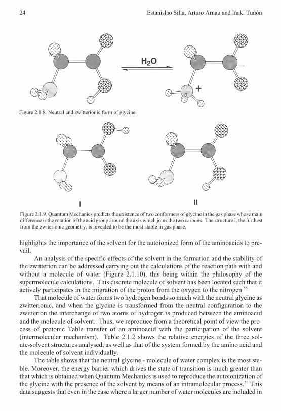
A practical case to compare the advantages obtained with the utilization of the differentmodels can be found in the autoionization of the aminoacids in aqueous solution. The chem-istry of the aminoacids in an aqueous medium has been at the forefront of numerous stud-ies,51-57 due to its self-evident biological interest. Thanks to these studies, it is well knownthat, whilst in the gas phase the aminoacids exist as non-autoionized structures, in aqueoussolution it is the zwiterionic form which is prevailing (Figure 2.1.8).

This transformation suggests that when an aminoacid molecule is introduced fromvacuum into the middle of a polar medium, which is the case of the physiological cellularmedia, a severe change is produced in its properties, its geometry, its energy, the chargeswhich its atoms support, the dipolar molecular moment, etc., set off and conditioned by thepresence of the solvent.

Utilizing Quantum Mechanics to analyze the geometry of the glycine in the absence ofsolvent, two energy minima are obtained (Figure 2.1.9), differentiated essentially by the ro-tation of the acid group. One of them is the absolute energy minimum in the gas phase (I),and the other is the conformation directly related with the ionic structure (II): The structurewhich is furthest from the zwiterionic form, I, is 0.7 Kcal/mol more stable than II, which


Figure 2.1.7. The Solvent Excluding Surface of a particular solute is the envelope of the volume excluded to thesolvent considered as a whole sphere that represents its charge density.

highlights the importance of the solvent for the autoionized form of the aminoacids to pre-vail.

An analysis of the specific effects of the solvent in the formation and the stability ofthe zwitterion can be addressed carrying out the calculations of the reaction path with andwithout a molecule of water (Figure 2.1.10), this being within the philosophy of thesupermolecule calculations. This discrete molecule of solvent has been located such that itactively participates in the migration of the proton from the oxygen to the nitrogen.55

That molecule of water forms two hydrogen bonds so much with the neutral glycine aszwitterionic, and when the glycine is transformed from the neutral configuration to thezwitterion the interchange of two atoms of hydrogen is produced between the aminoacidand the molecule of solvent. Thus, we reproduce from a theoretical point of view the pro-cess of protonic Table transfer of an aminoacid with the participation of the solvent(intermolecular mechanism). Table 2.1.2 shows the relative energies of the three sol-ute-solvent structures analysed, as well as that of the system formed by the amino acid andthe molecule of solvent individually.

The table shows that the neutral glycine - molecule of water complex is the most sta-ble. Moreover, the energy barrier which drives the state of transition is much greater thanthat which is obtained when Quantum Mechanics is used to reproduce the autoionization ofthe glycine with the presence of the solvent by means of an intramolecular process.55 Thisdata suggests that even in the case where a larger number of water molecules are included in


Figure 2.1.8. Neutral and zwitterionic form of glycine.

Figure 2.1.9. Quantum Mechanics predicts the existence of two conformers of glycine in the gas phase whose maindifference is the rotation of the acid group around the axis which joins the two carbons. The structure I, the furthestfrom the zwiterionic geometry, is revealed to be the most stable in gas phase.

the supermolecule calculation, the intramolecular mechanism will still continue as the pre-ferred in the autoionization of the glycine. The model of supermolecule has been useful tous, along with the competition of other models,54,55 to shed light on the mechanism by whichan aminoacid is autoionized in aqueous solution.

If the calculations are done again but this time including the presence of the solvent bymeans of a continuum model (implemented by means of a dielectric constant = 78.4; for thewater), the situation becomes different.55,58-60 Now it is the conformation closest to the zwit-terionic (II) which is the most stable, by some 2.7 Kcal/mol. This could be explained on thebasis of the greater dipolar moment of the structure (6.3 Debyes for the conformation IIcompared to 1.3 of the conformation I).

The next step was to reproduce the formation of the zwitterion starting with the moststable initial structure in the midst of the solvent (II). Using the continuum model, we ob-serve how the structure II evolves towards a state of transition which, once overcome, leads


Figure 2.1.10. Intramolecular and intermolecular proton transfer in glycine, leading from the neutral form to thezwitterionic one.

Table 2.1.2. Relative energies (in Kcal/mol) for the complexes formed between amolecule of water with the neutral glycine (NE·H2O), the zwitterion (ZW·H2O), and thestate of transition (TS·H2O), as well as for the neutral glycine system and independentmolecule of water (NE+H2O), obtained with a base HF/6-31+G**

NE·H2O TS·H2O ZW·H2O NE+H2O

0 29.04 16.40 4.32

to the zwitterion (Figure 2.1.7). This transition structure corresponds, then, to anintramolecular protonic transfer from the initial form to the zwiterionic form of theaminoacid. The calculations carried out reveal an activation energy of 2.39 Kcal/mol, and areaction energy of -1.15 Kcal/mol at the MP2/6-31+G** level.

A more visual check of the process submitted to study is achieved by means of hybridQM/MM Molecular Dynamics,58 which permits “snapshots” to be obtained which repro-duce the geometry of the aminoacid surrounded by the solvent. In Figure 2.1.11 are shownfour of these snapshots , corresponding to times of 200, 270, 405 and 440 femtoseconds af-ter commencement of the process.

In the first of these, the glycine has still not been autoionized. Two molecules of water(identified as A and B) form hydrogen bonds with the nitrogen of the amine group, whilst


Figure 2.1.11. The microscopic environment in which the formation of zwitterion takes place is exhibited in thesefour “snapshots”. It is possible to see the re-ordering of the structure of the molecule of glycine, along with there-ordering of the shell of molecules of water which surround it, at 200, 270, 405 and 440 femtoseconds from thebeginning of the simulation of the process by Molecular Dynamics.

only one (D) joins by hydrogen bond with the O2. Two more molecules of water (C and E)appear to stabilize electrostatically the hydrogen of the acid (H1). The second snapshot hasbeen chosen whilst the protonic transfer was happening. In this, the proton (H1) appearsjumping from the acid group to the amine group. However, the description of the first shellof hydratation around the nitrogen atoms, oxygen (O2) and of the proton in transit remain es-sentially unaltered with respect to the first snapshot. In the third snapshot the aminoacid hasnow reached the zwiterionic form, although the solvent still has not relaxed to its surround-ings. Now the molecules of water A and B have moved closer to the atom of nitrogen, and athird molecule of water appears imposed between them. At the same time, two molecules ofwater (D and E) are detected united clearly by bridges of hydrogen with the atom of oxygen(O2). All of these changes could be attributed to the charges which have been placed on theatoms of nitrogen and oxygen. The molecule of water (C) has followed a proton in its transitand has fitted in between this and the atom of oxygen (O2). In the fourth snapshot of the Fig-ure 2.1.8 the relaxing of the solvent, after the protonic transfer, is now observed, permittingthe molecule of water (C) to appear better orientated between the proton transferred (H1)and the atom of oxygen (O2), and this now makes this molecule of solvent strongly attachedto the zwitterion inducing into it appreciable geometrical distortions.

From the theoretical analysis carried out it can be inferred that the neutral conformerof the glycine II, has a brief life in aqueous solution, rapidly evolving to the zwitterionicspecies. The process appears to happen through an intramolecular mechanism and comesaccompanied by a soft energetic barrier. For its part, the solvent plays a role which is crucialboth to the stabilization of the zwitterion as well as to the protonic transfer. This latter is fa-vored by the fluctuations which take place in the surroundings.

2.1.4 THERMODYNAMIC AND KINETIC CHARACTERISTICS OF CHEMICALREACTIONS IN SOLUTION

It is very difficult for a chemical equilibrium not to be altered when passing from gas phaseto solution. The free energy standard of reaction, ∆Gº, is usually different in the gas phasecompared with the solution, because the solute-solvent interactions usually affect the reac-tants and the products with different results. This provokes a displacement of the equilib-rium on passing from the gas phase to the midst of the solution.

In the same way, and as was foreseen in section 2.1.1, the process of dissolution mayalter both the rate and the order of the chemical reaction. For this reason it is possible to usethe solvent as a tool both to speed up and to slow down the development of a chemical pro-cess.

Unfortunately, little experimental information is available on how the chemical equi-libria and the kinetics of the reactions become altered on passing from the gas phase to thesolution, since as commented previously, the techniques which enable this kind of analysisare relatively recent. It is true that there is abundant experimental information, nevertheless,on how the chemical equilibrium and the velocity of the reaction are altered when one sameprocess occurs in the midst of different solvents.

2.1.4.1 Solvent effects on chemical equilibria

The presence of the solvent is known to have proven influences in such a variety of chemi-cal equilibria: acid-base, tautomerism, isomerization, association, dissociation,conformational, rotational, condensation reactions, phase-transfer processes, etc.,1 that itsdetailed analysis is outside the reach of a text such as this. We will limit ourselves to analyz-


ing superficially the influence that the solvent has on one of the equilibria of greatest rele-vance, the acid-base equilibrium.

The solvent can alter an acid-base equilibrium not only through the acid or basic char-acter of the solvent itself, but also by its dielectric effect and its capacity to solvate the dif-ferent species which participate in the process. Whilst the acid or basic force of a substancein the gas phase is an intrinsic characteristic of the substance, in solution this force is also areflection of the acid or basic character of the solvent and of the actual process of solvat-ation. For this reason the scales of acidity or basicity in solution are clearly different fromthose corresponding to the gas phase. Thus, toluene is more acid than water in the gas phasebut less acid in solution. These differences between the scales of intrinsic acidity-basicityand in solution have an evident repercussion on the order of acidity of some series of chemi-cal substances. Thus, the order of acidity of the aliphatic alcohols becomes inverted on pass-ing from the gas phase to solution:

The protonation free energies of MeOH to t-ButOH have been calculated in gas phaseand with a continuum model of the solvent.61 It has been shown that in this case continuummodels gives solvation energies which are good enough to correctly predict the acidity or-dering of alcohols in solution. Simple electrostatic arguments based on the chargedelocalization concept, were used to rationalize the progressive acidity of the alcohols whenhydrogen atoms are substituted by methyl groups in the gas phase, with the effect on the so-lution energies being just the opposite. Thus, both the methyl stabilizing effect and the elec-trostatic interaction with the solvent can explain the acid scale in solution. As both terms arerelated to the molecular size, this explanation could be generalized for acid and base equi-libria of homologous series of organic compounds:

AH ⇔ A- + H+

B + H+ ⇔ BH+

In vacuo, as the size becomes greater by adding methyl groups, displacement of theequilibria takes place toward the charged species. In solution, the electrostatic stabilizationis lower when the size increases, favoring the displacement of the equilibria toward the neu-tral species. The balance between these two tendencies gives the final acidity or basicity or-dering in solution. Irregular ordering in homologous series are thus not unexpected takinginto account the delicate balance between these factors in some cases.62

2.1.4.2 Solvent effects on the rate of chemical reactions

When a chemical reaction takes place in the midst of a solution this is because, prior to this,the molecules of the reactants have diffused throughout the medium until they have met.This prior step of the diffusion of the reactants can reach the point of conditioning the per-formance of the reaction, especially in particularly dense and/or viscous surroundings. Thisis the consequence of the liquid phase having a certain microscopic order which, although


in gas phase:

in solution:

R CH2 OH R CH OH

R'

R C OH

R'

R''

R CH2 OH R C OH

R'

R''

R CH OH

R'

< <

> >

much less than that of the solid state, is not depreciable. Thus, in a solution, each moleculeof solute finds itself surrounded by a certain number of molecules of solvent which enve-lope it forming what has been denominated as the solvent cage. Before being able to escapefrom the solvent cage each molecule of solute collides many times with the molecules ofsolvent which surround it.

In the case of a dilute solution of two reactants, A and B, their molecules remain for acertain time in a solvent cage. If the time needed to escape the solvent cage by the moleculesA and B is larger than the time needed to suffer a bimolecular reaction, we can say that thiswill not find itself limited by the requirement to overcome an energetic barrier, but that thereaction is controlled by the diffusion of the reactants. The corresponding reaction rate will,therefore, have a maximum value, known as diffusion-controlled rate. It can be demon-strated that the diffusion-limited bimolecular rate constants are of the order of 1010-1011

M-1s-1, when A and B are ions with opposite charges.63 For this reason, if a rate constant is ofthis order of magnitude, we must wait for the reaction to be controlled by the diffusion of thereactants. But, if the rate constant of a reaction is clearly less than the diffusion-limitedvalue, the corresponding reaction rate is said to be chemically controlled.

Focusing on the chemical aspects of the reactivity, the rupture of bonds which goesalong with a chemical reaction usually occurs in a homolytic manner in the gas phase. Forthis reason, the reactions which tend to prevail in this phase are those which do not involve aseparation of electric charge, such as those which take place with the production of radicals.In solution, the rupture of bonds tends to take place in a heterolytic manner, and the solventis one of the factors which determines the velocity with which the process takes place. Thisexplains that the reactions which involve a separation or a dispersion of the electric chargecan take place in the condensed phase. The effects of the solvent on the reactions which in-volve a separation of charge will be very drawn to the polar nature of the state of transitionof the reaction, whether this be a state of dipolar transition, isopolar or of the free-radicaltype. The influence of the solvent, based on the electric nature of the substances which arereacting, will also be essential, and reactions may occur between neutral nonpolar mole-cules, between neutral dipolar molecules, between ions and neutral nonpolar molecules, be-tween ions and neutral polar molecules, ions with ions, etc. Moreover, we should bear inmind that alongside the non specific solute-solvent interactions (electrostatic, polarization,dispersion and repulsion), specific interactions may be present, such as the hydrogen bonds.


Table 2.1.3. Relative rate constants of the Menschutkin reaction betweentriethylamine and iodoethane in twelve solvents at 50oC. In 1,1,1-trichloroethane therate constant is 1.80×10-5 l mol-1 s-1. Data taken from reference 40

SolventRelative rate

constantSolvent

Relative rateconstant

1,1,1-Trichloroethane 1 Acetone 17.61

Chlorocyclohexane 1.72 Cyclohexanone 18.72

Chlorobenzene 5.17 Propionitrile 33.11

Chloroform 8.56 Benzonitrile 42.50

1,2-Dichlorobenzene 10.06

The influence of the solvent on the rate at which a chemical reaction takes place wasalready made clear, in the final stages of the XIX century, with the reaction of Menschutkinbetween tertiary amines and primary haloalkanes to obtain quaternary ammonium salts.64

The reaction of Menschutkin between triethylamine and iodoethane carried out in differentmedia shows this effect (Table 2.1.3):

2.1.4.3 Example of application: addition of azide anion to tetrafuranosides

The capacity of the solvent to modify both the thermodynamic and also the kinetic aspectsof a chemical reaction are observed in a transparent manner on studying the stationary struc-tures of the addition of azide anion to tetrafuranosides, particularly: methyl2,3-dideoxy-2,3-epimino-α-L-erythrofuranoside (I), methyl 2,3-anhydro-α-L-erythro-furanoside (II), and 2,3-anhydro-β-L-erythrofuranoside (III). An analysis with molecularorbital methods at the HF/3-21G level permits the potential energy surface in vacuo to becharacterized, to locate the stationary points and the possible reaction pathways.65 The ef-fect of the solvent can be implemented with the aid of a polarizable continuum model. Fig-ure 2.1.12 shows the three tetrafuranosides and the respective products obtained when azideanion attacks in C3 (P1) or in C4 (P2).

The first aim of a theoretical study of a chemical reaction is to determine the reactionmechanism that corresponds to the minimum energy path that connects the minima of reac-tant and products and passes through the transition state (TS) structures on the potential en-


Figure 2.1.12. Models of the reaction studied for the addition of azide anion to tetrafuranosides. The experimentalproduct ratio is also given.

ergy surface. In this path the height of the barrier that exists between the reactant and TS iscorrelated to the rate of each different pathway (kinetic control), while the relative energy ofreactants and products is correlated to equilibrium parameters (thermodynamic control).The second aim is how the solute-solvent interactions affect the different barrier heights andrelative energies of products, mainly when charged or highly polar structures appear alongthe reaction path. In fact, the differential stabilization of the different stationary points in thereaction paths can treat one of them favorably, sometimes altering the relative energy orderfound in vacuo and, consequently, possibly changing the ratio of products of the reaction.An analysis of the potential energy surface for the molecular model I led to the location ofthe stationary points showed in Figure 2.1.13.

The results obtained for the addition of azide anion to tetrafuranosides with differentmolecular models and in different solvents can be summarized as follows:65

• For compound I, in vacuo, P1 corresponds to the path with the minimum activationenergy, while P2 is the more stable product (Figures 2.1.14 and 2.1.15). When thesolvent effect is included, P1 corresponds to the path with the minimum activationenergy and it is also the more stable product. For compound II, in vacuo, P2 is themore stable product and also presents the smallest activation energy. The inclusionof the solvent effect in this case changes the order of products and transition statesstability. For compound III, P1 is the more stable product and presents the smallestactivation energy both in vacuo and in solution.

• A common solvent effect for the three reactions is obtained: as far as the dielectricconstant of the solvent is augmented, the energy difference between P1 and P2


Figure 2.1.13. Representation of the stationary points (reactants, reactant complex, transition states, and products)for the molecular mechanism of compound I. For the TS´s the components of the transition vectors are depicted byarrows.

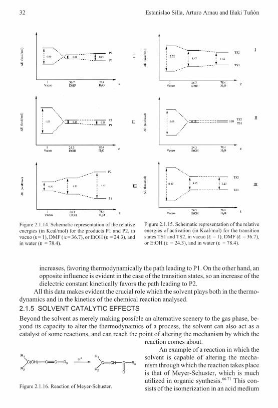
increases, favoring thermodynamically the path leading to P1. On the other hand, anopposite influence is evident in the case of the transition states, so an increase of thedielectric constant kinetically favors the path leading to P2.

All this data makes evident the crucial role which the solvent plays both in the thermo-dynamics and in the kinetics of the chemical reaction analysed.

2.1.5 SOLVENT CATALYTIC EFFECTS

Beyond the solvent as merely making possible an alternative scenery to the gas phase, be-yond its capacity to alter the thermodynamics of a process, the solvent can also act as acatalyst of some reactions, and can reach the point of altering the mechanism by which the

reaction comes about.An example of a reaction in which the

solvent is capable of altering the mecha-nism through which the reaction takes placeis that of Meyer-Schuster, which is muchutilized in organic synthesis.66-71 This con-sists of the isomerization in an acid medium


Figure 2.1.14. Schematic representation of the relativeenergies (in Kcal/mol) for the products P1 and P2, invacuo (ε= 1), DMF ( ε= 36.7), or EtOH (ε = 24.3), andin water (ε = 78.4).

Figure 2.1.15. Schematic representation of the relativeenergies of activation (in Kcal/mol) for the transitionstates TS1 and TS2, in vacuo (ε = 1), DMF (ε = 36.7),or EtOH (ε = 24.3), and in water (ε = 78.4).

Figure 2.1.16. Reaction of Meyer-Schuster.

of secondary and tertiaryα-acetylenic alcohols to carbon-ylic α β, -unsaturated compounds(Figure 2.1.16).

Its mechanism consists ofthree steps (Figure 2.1.17). Thefirst one is the protonation of theoxygen atom. The second, whichdetermines the reaction rate, isthat in which the 1.3 shift from theprotonated hydroxyl group is pro-duced through the triple bond togive way to the structure of alenol.The last stage corresponds to thedeprotonation of the alenol, pro-ducing a keto-enolic tautomerismwhich displaces towards theketonic form.

For the step which limits thereaction rate (rate limiting step),three mechanisms have been pro-

posed, two of which are intramolecular - denominated intramolecular, as such, andsolvolytic - and the other intermolecular (Figure 2.1.18). The first of these implies a cova-lent bond between water and the atoms of carbon during the whole of the transposition. Inthe solvolytic mechanism there is an initial rupture from the O-C1 bond, followed by anucleophilic attack of the H2O on the C3. Whilst the intermolecular mechanism correspondsto a nucleophilic attack of H2O on the terminal carbon C3 and the loss of the hydroxyl groupprotonated of the C1.

The analysis of the first two mechanisms showed72 the solvolytic mechanism as themost favorable localizing itself during the reaction path to an alquinylic carbocation inter-acting electrostatically with a molecule of water. This fact has been supported by the exper-imental detection of alquinylic carbocations in solvolytic conditions. Things being like that,two alternatives remain for the slow stage of the Meyer-Schuster reaction, the solvolyticand the intermolecular mechanism, and it seems that the solvent has a lot to say in this.

Although both mechanisms evolve in two steps, these are notably different. In theintermolecular mechanism, the first transition state can be described as an almost pure elec-trostatic interaction of the entrant molecule of water with the C3, whilst the C1 remainsunited covalently to the protonated hydroxyl group. This first transition state leads to a in-termediate in which the two molecules of water are covalently bonded to the C1 and C3 at-oms. The step from the intermediate to the product takes place through a second transitionstate, in which the C3 is covalently bonded to the molecule of entrant water and there is anelectrostatic interaction of the other water molecule. In the mechanism which we callsolvolytic, the first transition state corresponds to the pass from covalent to electrostatic in-teraction of the H2O united to the C1, that is to say, to a process of solvolysis, so, the watermolecule remains interacting electrostatically with the carbons C1 and C3.


Figure 2.1.17. Steps of the reaction of Meyer-Schuster.

On comparing the solvolytic and intermolecular processes a smaller potential barrieris observed for the latter, thus the solvent plays an active part in the Meyer-Schuster reac-tion, being capable of changing radically the mechanism through which this takes place. Itseems clear that in the presence of aqueous solvents the nucleophilic attack on the C3 pre-cedes the loss of the water (solvolysis): a lesser activation energy corresponds to theintermolecular process than to the solvolytic. Moreover, if we analyze the intermolecularmechanism we can verify that the solvent stabilizes both the reactants as well as the prod-ucts by the formation of hydrogen bridges.

EpilogueAs a fish in the midst of the ocean, the reactants are usually found in the midst of a solutionin our laboratory tests. In the same way as in the ocean where there is both danger and aheaven for the fish, in the internal scenery of a solution the chemical reactions can bespeeded up or slowed down, favored thermodynamically or prejudiced. In this way, onpassing from vacuum to a solution, the molecules of the reactants can experience alterationsin their geometry, the distribution of their charges, or their energy, which can have an effecton the outcome of the reaction. In the preceding pages we have attempted to make clearthese solute-solvent influences, and to achieve this we have plunged, hand in hand with the-oretical chemistry, into the microscopic and recondite environment of the solutions.

REFERENCES

1 Ch. Reichardt, Solvents and Solvent Effects in Organic Chemistry, VCH, Weinheim, 1988, p. 1.2 H. Metzger, Newton, Stahl, Boerhaave et la doctrine chimique, Alcan, Paris, 1930, pp. 280-289.3 M.M. Pattison, A History of Chemical Theories and Laws, John Wiley & Sons, New York, 1907, p. 381.4 H.M. Leicester, Panorama histórico de la química, Alhambra, Madrid, 1967, pp. 148, 149. (Transcription

from: The Historical Background of Chemistry, John Wiley & Sons, New York.)5 J.L. Proust, J. Phys., 63, 369, 1806.6 M. Berthelot and L. Péan de Saint-Gilles, Ann. Chim. et Phys., Ser. 3, 65, 385 (1862); 66, 5 (1862); 68, 255

(1863).7 N. Menschutkin, Z. Phys. Chem., 6, 41 (1890).8 E. D. Hughes, C. K. Ingold, J. Chem. Soc., 244, 252 (1935).9 L. Claisen, Liebigs Ann. Chem., 291, 25 (1896).


Figure 2.1.18. Three different mechanism for the rate-limiting step of the reaction of Meyer-Schuster.

10 W. Wislicenus. Liebigs Ann. Chem., 291, 147 (1896).11 J. E. Bartmess, J. A. Scott, R. T. McIver Jr., J. Am. Chem. Soc., 101, 6056 (1979).12 L. M. Jackman, D. P. Kelly, J. Chem. Soc., (B) 102 (1970).13 H. C. Brown, H. Bartholomay, M. D. Taylor, J. Am. Chem. Soc., 66, 435 (1944).14 J. P. Briggs, R. Yamdagni, P. Kebarle, J. Am. Chem. Soc., 94, 5128 (1972).15 T. A. Leheman, M. M. Bursey, Ion Cyclotron Resonance Spectrometry, Wiley, New York, 1976.16 S. A. McLukey, D. Cameron, R. G. Cooks, J. Am. Chem. Soc., 103, 1313 (1981).17 B. K. Bohme, P. Fennelly, R. S: Hemsworth, H. J. Schiff, J. Am. Chem. Soc. b, 7512 (1973).18 J. E. Bartmess, R. T. McIver, Gas phase Ion Chemistry, M. T. Bowe ed., Ed., Academic Press, New York,

1979.19 J. W. Larson, T. B. McMahon, J. Am. Chem. Soc., 104, 6255 (1982).20 M. Meotner, L. W: Sieck, J. Am. Chem. Soc., 105, 2956 (1983).21 C. L. Brooks III, M. Karplus, Methods Enzymol., 127, 369 (1986).22 D. Beece, L. Eisenstein, H. Frauenfelder, D. Good, M. C. Marden, L. Reinisch, A. H. Reynolds,

L. B. Sorensen, K. T. Yue, Biochemistry, 19, 5147 (1980).23 J.E. Lennard-Jones, Proc. Phys. Soc. London, 43, 461 (1931).24 J. P. Daudey, Int. J. Quantum Chem., b, 29 (1974); J. L. Rivail, Éléments de Chimie Quantique à l’usage

des Chimistes, InterÉditions-CNRS Éditions, Paris (1994).25 C. Sandorfy, R. Buchet, L.S. Lussier, P. Ménassa and L. Wilson, Pure Appl. Chem., 58, 1115 (1986).

J. N., Israelachvili, Intermolecular and surface forces, Academic Press, San Diego, 1989.26 W. Kauzmann, Adv. Protein Chem., 14, 1 (1959).27 H. S. Frank and M. W. Evans, J. Chem. Phys., 13, 507 (1945).28 W. Blokzilj and J. B. F. N. Engberts, Angew. Chem. Int. Ed. Engl., 32, 1545 (1993).29 B. Lee, Biopolymers, 24, 813 (1985), B. Lee, Biopolymers, 31, 993 (1991).30 W. L. Jorgensen, J. K. Bukner, S. Boudon and J. Tirado-Rives, Chem. Phys., 89, 3742 (1988); C. Pangali,

M. Rao and B. J. Berne, J. Chem. Phys., 71, 2975(1979); D. van Belle and S. J. Wodak, J. Am. Chem. Soc.,115, 647 (1993); M. H. New and B. J. Berne, J. Am. Chem. Soc., 117, 7172 (1995); D. E. Smith, L. Zhang andA. D. J. Haymet, J. Am. Chem. Soc., 114, 5875 (1992); ); D. E. Smith and A. D. J. Haymet, J. Chem. Phys.,98, 6445(1994); L. X. Dang, J. Chem. Phys., 100, 9032(1994); T. Head-Gordon, Chem. Phys. Lett., 227, 215(1994).

31 J. Pitarch, V. Moliner, J. L. Pascual-Ahuir, E. Silla and I. Tuñçon , J. Phys. Chem., 100, 9955(1996).32 J. Tomasi and M. Persico, Chem. Rev., 94, 2027-2094 (1994).33 A. Rahman and F.M. Stillinger, J. Chem. Phys., 57, 3336 (1971). A. R. Leach, Molecular Modelling,

Addison Wesley Longman, Singapore, 1997.34 B.J. Alder and T.E. Wainwright, J. Chem. Phys., 27, 1208-1209 (1957).35 N. Metropolis, A.W. Rosenbluth, M.N. Rosenbluth, A. Teller and E. Teller, J. Chem. Phys., 21, 1087 (1953)36 A. Warshel, M. Levitt, J. Mol. Biol., 103, 227-249 (1973). P. A. Bash, M. J. Field, M. Karplus, J. Am. Chem.

Soc., 109, 8092-8094 (1987).37 M. Born, Z. Physik, 1, 45 (1920); J. G. Kirkwood, J. Chem. Phys., 2, 351 (1934); J. G. Kirkwood,

F. H. Westheimer, J. Chem. Phys., 6, 506 (1936); L. Onsager, J. Am. Chem. Soc., 58, 1486 (1936).38 E. Scrocco, J. Tomasi, Top. Curr. Chem., 42, 97 (1973). J. L. Pascual-Ahuir, E. Silla, J. Tomasi,

R. Bonaccorsi, J. Comput. Chem., 8, 778 (1987).39 D. Rinaldi, J. L. Rivail, N. Rguini, J. Comput. Chem., b, 676 (1992).40 I. Tuñón, E. Silla, J. Bertrán, J. Chem. Soc. Fraday Trans., 90, 1757 (1994).41 X. Assfeld, D. Rinaldi, AIP Conference Proceedings ECCC1, F. Bernardi, J. L. Rivail, Eds., AIP, Woodbury,

New York, 1995.42 F. M. Floris, J. Tomasi, J. L. Pascual Ahuir, J. Comput. Chem., 12, 784 (1991); C. J. Cramer and

D. G. Trhular, Science, 256, 213 (1992); V. Dillet, D. Rinaldi, J. G. Angyan and J. L. Rivail, Chem. Phys.Lett., 202, 18 (1993).

43 I. Tuñón, E. Silla, J. L. Pascual-Ahuir, Prot. Eng., 5, 715 (1992); I. Tuñón, E. Silla, J. L. Pascual-Ahuir,Chem. Phys. Lett., 203, 289 (1993); R. B. Hermann, J. Phys. Chem., 76, 2754 (1972); K. A. Sharp,A. Nicholls, R. F: Fine, B. Honig, Science, 252, 106 (1991).

44 L. H. Pearl, A. Honegger, J. Mol. Graphics, 1, 9 (1983); R. Voorintholt, M. T. Kosters, G. Vegter, G. Vriend,W. G. H. Hol, J. Mol. Graphics, 7, 243 (1989); J. B. Moon, W. J. Howe, J. Mol. Graphics, 7, 109 (1989);E. Silla, F. Villar, O. Nilsson, J.L. Pascual-Ahuir, O. Tapia, J. Mol. Graphics, 8, 168 (1990).

45 B. Lee, F. M. Richards, J. Mol. Biol., 55, 379 (1971).46 F. M. Richards, Ann. Rev. Biophys. Bioeng., 6, 151 (1977).47 J. L. Pascual-Ahuir, E. Silla, I. Tuñón, J. Comput. Chem., 15, 1127-1138 (1994).


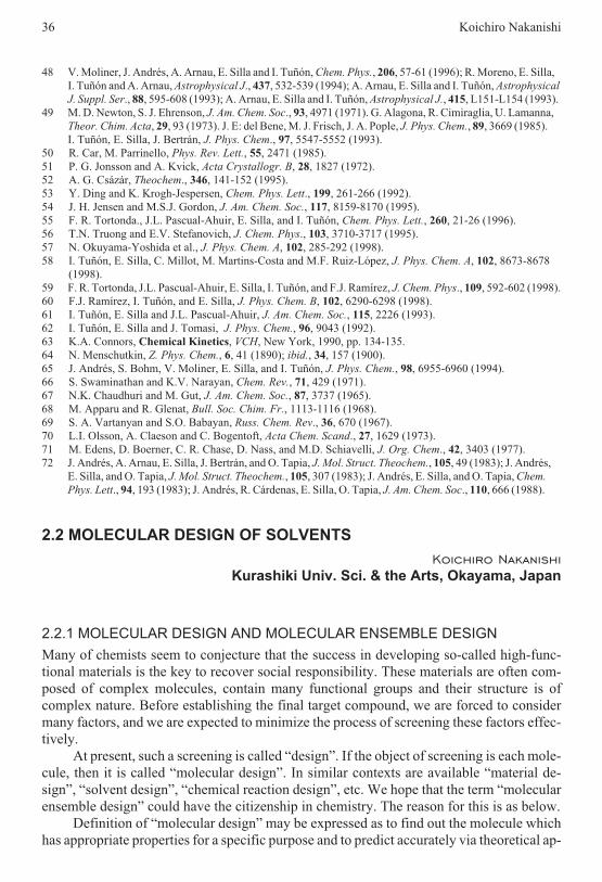
48 V. Moliner, J. Andrés, A. Arnau, E. Silla and I. Tuñón, Chem. Phys., 206, 57-61 (1996); R. Moreno, E. Silla,I. Tuñón and A. Arnau, Astrophysical J., 437, 532-539 (1994); A. Arnau, E. Silla and I. Tuñón, AstrophysicalJ. Suppl. Ser., 88, 595-608 (1993); A. Arnau, E. Silla and I. Tuñón, Astrophysical J., 415, L151-L154 (1993).

49 M. D. Newton, S. J. Ehrenson, J. Am. Chem. Soc., 93, 4971 (1971). G. Alagona, R. Cimiraglia, U. Lamanna,Theor. Chim. Acta, 29, 93 (1973). J. E: del Bene, M. J. Frisch, J. A. Pople, J. Phys. Chem., 89, 3669 (1985).I. Tuñón, E. Silla, J. Bertrán, J. Phys. Chem., 97, 5547-5552 (1993).

50 R. Car, M. Parrinello, Phys. Rev. Lett., 55, 2471 (1985).51 P. G. Jonsson and A. Kvick, Acta Crystallogr. B, 28, 1827 (1972).52 A. G. Csázár, Theochem., 346, 141-152 (1995).53 Y. Ding and K. Krogh-Jespersen, Chem. Phys. Lett., 199, 261-266 (1992).54 J. H. Jensen and M.S.J. Gordon, J. Am. Chem. Soc., 117, 8159-8170 (1995).55 F. R. Tortonda., J.L. Pascual-Ahuir, E. Silla, and I. Tuñón, Chem. Phys. Lett., 260, 21-26 (1996).56 T.N. Truong and E.V. Stefanovich, J. Chem. Phys., 103, 3710-3717 (1995).57 N. Okuyama-Yoshida et al., J. Phys. Chem. A, 102, 285-292 (1998).58 I. Tuñón, E. Silla, C. Millot, M. Martins-Costa and M.F. Ruiz-López, J. Phys. Chem. A, 102, 8673-8678

(1998).59 F. R. Tortonda, J.L. Pascual-Ahuir, E. Silla, I. Tuñón, and F.J. Ramírez, J. Chem. Phys., 109, 592-602 (1998).60 F.J. Ramírez, I. Tuñón, and E. Silla, J. Phys. Chem. B, 102, 6290-6298 (1998).61 I. Tuñón, E. Silla and J.L. Pascual-Ahuir, J. Am. Chem. Soc., 115, 2226 (1993).62 I. Tuñón, E. Silla and J. Tomasi, J. Phys. Chem., 96, 9043 (1992).63 K.A. Connors, Chemical Kinetics, VCH, New York, 1990, pp. 134-135.64 N. Menschutkin, Z. Phys. Chem., 6, 41 (1890); ibid., 34, 157 (1900).65 J. Andrés, S. Bohm, V. Moliner, E. Silla, and I. Tuñón, J. Phys. Chem., 98, 6955-6960 (1994).66 S. Swaminathan and K.V. Narayan, Chem. Rev., 71, 429 (1971).67 N.K. Chaudhuri and M. Gut, J. Am. Chem. Soc., 87, 3737 (1965).68 M. Apparu and R. Glenat, Bull. Soc. Chim. Fr., 1113-1116 (1968).69 S. A. Vartanyan and S.O. Babayan, Russ. Chem. Rev., 36, 670 (1967).70 L.I. Olsson, A. Claeson and C. Bogentoft, Acta Chem. Scand., 27, 1629 (1973).71 M. Edens, D. Boerner, C. R. Chase, D. Nass, and M.D. Schiavelli, J. Org. Chem., 42, 3403 (1977).72 J. Andrés, A. Arnau, E. Silla, J. Bertrán, and O. Tapia, J. Mol. Struct. Theochem., 105, 49 (1983); J. Andrés,

E. Silla, and O. Tapia, J. Mol. Struct. Theochem., 105, 307 (1983); J. Andrés, E. Silla, and O. Tapia, Chem.Phys. Lett., 94, 193 (1983); J. Andrés, R. Cárdenas, E. Silla, O. Tapia, J. Am. Chem. Soc., 110, 666 (1988).

2.2 MOLECULAR DESIGN OF SOLVENTS

Koichiro Nakanishi

Kurashiki Univ. Sci. & the Arts, Okayama, Japan

2.2.1 MOLECULAR DESIGN AND MOLECULAR ENSEMBLE DESIGN

Many of chemists seem to conjecture that the success in developing so-called high-func-tional materials is the key to recover social responsibility. These materials are often com-posed of complex molecules, contain many functional groups and their structure is ofcomplex nature. Before establishing the final target compound, we are forced to considermany factors, and we are expected to minimize the process of screening these factors effec-tively.

At present, such a screening is called “design”. If the object of screening is each mole-cule, then it is called “molecular design”. In similar contexts are available “material de-sign”, “solvent design”, “chemical reaction design”, etc. We hope that the term “molecularensemble design” could have the citizenship in chemistry. The reason for this is as below.

Definition of “molecular design” may be expressed as to find out the molecule whichhas appropriate properties for a specific purpose and to predict accurately via theoretical ap-

36 Koichiro Nakanishi

proach the properties of the molecule. If the molecular system in question consists of an iso-lated free molecule, then it is “molecular design”. If the properties are of complexmacroscopic nature, then it is “material design”. Problem remains in the intermediate be-tween the above two. Because fundamental properties shown by the ensemble of moleculesare not always covered properly by the above two types of design. This is because the mo-lecular design is almost always based on quantum chemistry of free molecule and the mate-rial design relies too much on empirical factor at the present stage. When we proceed tomolecular ensemble (mainly liquid phase), as the matter of fact, we must use statistical me-chanics as the basis of theoretical approach.

Unfortunately, statistical mechanics is not familiar even for the large majority ofchemists and chemical engineers. Moreover, fundamental equations in statistical mechan-ics cannot often be solved rigorously for complex systems and the introduction of approxi-mation becomes necessary to obtain useful results for real systems. In any theoreticalapproach for molecular ensemble, we must confront with so-called many-body problemsand two-body approximations must be applied. Even in the frameworks of this approxima-tion, our knowledge on the intermolecular interaction, which is necessary in statistical me-chanical treatment is still poor.

Under such a circumstance, numerical method should often be useful. In the case ofstatistical mechanics of fluids, we have Monte Carlo (MC) simulation based on the Metrop-olis scheme. All the static properties can be numerically calculated in principle by the MCmethod.

Another numerical method to supplement the MC method should be the numerical in-tegration of the equations of motion. This kind of calculation for simple molecular systemsis called molecular dynamics (MD) method where Newton or Newton-Euler equation ofmotion is solved numerically and some dynamic properties of the molecule involved can beobtained.

These two methods are invented, respectively, by the Metropolis group (MC, Metrop-olis et al., 1953)1 and Alder’s group (MD, Alder et al., 1957)2 and they are the molecularversions of computer experiments and therefore called now molecular simulation.3 Molecu-lar simulation plays a central role in “molecular ensemble design”. They can reproducethermodynamics properties, structure and dynamics of a group of molecules by using highspeed supercomputer. Certainly any reasonable calculations on molecular ensemble needlong computer times, but the advance in computer makes it possible that this problem be-comes gradually less serious.

Rather, the assignment is more serious with intermolecular interaction potential used.For simple molecules, empirical model potential such as those based on Lennard-Jones po-tential and even hard-sphere potential can be used. But, for complex molecules, potentialfunction and related parameter value should be determined by some theoretical calcula-tions. For example, contribution of hydrogen-bond interaction is highly large to the total in-teraction for such molecules as H2O, alcohols etc., one can produce semi-empiricalpotential based on quantum-chemical molecular orbital calculation. Molecular ensembledesign is now complex unified method, which contains both quantum chemical and statisti-cal mechanical calculations.

2.2.2 FROM PREDICTION TO DESIGN

It is not new that the concept of “design” is brought into the field of chemistry. Moreover,essentially the same process as the above has been widely used earlier in chemical engineer-

2.2 Molecular design of solvents 37

ing. It is known as the prediction and correlation methods of physical properties, that is, themethod to calculate empirically or semi-empirically the physical properties, which is to beused in chemical engineering process design. The objects in this calculation include ther-modynamic functions, critical constant, phase equilibria (vapor pressure, etc.) for one-com-ponent systems as well as the transport properties and the equation of state. Also includedare physical properties of two-components (solute + pure solvent) and even of three-compo-nents (solute + mixed solvent) systems. Standard reference, “The properties of Gases andLiquids; Their Estimation and Prediction”,4 is given by Sherwood and Reid. It was revisedonce about ten years interval by Reid and others. The latest 4th edition was published in1987. This series of books contain excellent and useful compilation of “prediction” method.However, in order to establish the method for molecular ensemble design we need to followthree more stages.(1) Calculate physical properties of any given substance. This is just the establishment

and improvement of presently available “prediction” method.(2) Calculate physical properties of model-substance. This is to calculate physical

properties not for each real molecule but for “model”. This can be done bycomputer simulation. On this stage, compilation of model"substance data base willbe important.

(3) Predict real substance (or corresponding “model”) to obtain required physicalproperties. This is just the reverse of the stage (1) or (2). But, an answer in thisstage is not limited to one particular substance.

The scheme to execute these three stages for a large variety of physical properties andsubstances has been established only to a limited range. Especially, important is the estab-lishment of the third stage, and after that, “molecular ensemble design” will be worth to dis-cuss.

2.2.3 IMPROVEMENT IN PREDICTION METHOD

Thus, the development of “molecular ensemble design” is almost completely future assign-ment. In this section, we discuss some attempts to improve prediction at the level of stage(1). It is taken for the convenience’s sake from our own effort. This is an example of re-peated improvements of prediction method from empirical to molecular level.

The diffusion coefficient D1 of solute 1 in solvent 2 at infinitely dilute solution is a fun-damental property. This is different from the self-diffusion coefficient D0 in pure liquid.Both D1 and D0 are important properties. The classical approach to D1 can be done based onStokes and Einstein relation to give the following equation

D kT r1 2 16η π= / [2.2.1]

where D1 at constant temperature T can be determined by the radius r1 of solute moleculeand solvent viscosity η2 (k is the Boltzmann constant). However, this equation is valid onlywhen the size of solvent molecule is infinitely small, namely, for the diffusion in continuousmedium. It is then clear that this equation is inappropriate for molecular mixtures. The wellknown Wilke-Chang equation,5 which corrects comprehensively this point, can be used forpractical purposes. However, average error of about 10% is inevitable in the comparisonwith experimental data.


One attempt6 to improve the agreement with experimental data is to useHammond-Stokes relation in which the product D1η2 is plotted against the molar volume ra-tio of solvent to solute Vr. The slope is influenced by the following few factors, namely,

(1) self-association of solvent,(2) asymmetricity of solvent shape, and(3) strong solute-solvent interactions.

If these factors can be taken properly into account, the following equation is obtained.

D T K V K Vr T1 2 1 0

1 3

2η / / //= + [2.2.2]

Here constants K1 and K2 contain the parameters coming from the above factors andV0 is the molar volume of solute.

This type of equation [2.2.2] cannot be always the best in prediction, but physical im-age is clearer than with other purely empirical correlations. This is an example of the stage(1) procedure and in order to develop a stage (2) method, we need MD simulation data forappropriate model.

2.2.4 ROLE OF MOLECULAR SIMULATION

We have already pointed out that statistical mechanical method is indispensable in “molec-ular ensemble design”. Full account of molecular simulation is given in some books3 andwill not be reproduced here. Two types of approaches can be classified in applying thismethod.

The first one makes every effort to establish and use as real as exact intermolecular in-teraction in MC and MD simulation. It may be limited to a specific type of compounds. Thesecond is to use simple model, which is an example of so-called Occam’s razor. We may ob-tain a wide bird-view from there.

In the first type of the method, intermolecular interaction potential is obtained basedon quantum-chemical calculation. The method takes the following steps.(1) Geometry (interatomic distances and angles) of molecules involved is determined.

For fundamental molecules, it is often available from electron diffraction studies.Otherwise, the energy gradient method in molecular orbital calculation can beutilized.

(2) The electronic energy for monomer E1 and those for dimers of various mutualconfigurations E2 are calculated by the so-called ab initio molecular orbitalmethod, and the intermolecular energy E2-2E1 is obtained.

(3) By assuming appropriate molecular model and semi-empirical equation,parameters are optimized to reproduce intermolecular potential energy function.

Representative example of preparation of such potential energy function, called nowab initio potential would be MCY potential for water-dimer by Clementi et al.7 Later, simi-lar potentials have been proposed for hetero-dimer such as water-methanol.8 In the case ofsuch hydrogen-bonded dimers, the intermolecular energy E2-2E1 can be fairly large valueand determination of fitted parameters is successful. In the case of weak interaction, ab in-itio calculation needs long computer time and optimization of parameter becomes difficult.In spite of such a situation, some attempts are made for potential preparation, e.g., for ben-zene and carbon dioxide with limited success.

To avoid repeated use of long time MO calculation, Jorgensen et al.9 has proposedMO-based transferable potential parameters called TIPS potential. This is a potential ver-


sion of additivity rule, which has now an empirical character. It is however useful for practi-cal purposes.

2.2.5 MODEL SYSTEM AND PARADIGM FOR DESIGN

The method described above is so to speak an orthodox approach and the ability of pres-ent-day’s supercomputer is still a high wall in the application of molecular simulation. Thenthe role of the second method given in the last section is highly expected.

It is the method with empirical potential model. As the model, the approximation thatany molecule can behave as if obeying Lennard-Jones potential seems to be satisfactory.This (one-center) LJ model is valid only for rare gases and simple spherical molecules. Butthis model may also be valid for other simple molecules as a zeroth approximation. We mayalso use two-center LJ model where interatomic interactions are concentrated to the majortwo atoms in the molecule. We expect that these one-center and two-center LJ models willplay a role of Occam’s razor.

We propose a paradigm for physical properties prediction as shown in Figure 2.2.1.This corresponds to the stage (2) and may be used to prepare the process of stage (3),namely, the molecular ensemble design for solvents.

Main procedures in this paradigm are as follows; we first adopt target molecule ormixture and determine their LJ parameters. At present stage, LJ parameters are availableonly for limited cases. Thus we must have method to predict effective LJ parameters.


Figure 2.2.1. A scheme for the design of molecular ensembles.

For any kinds of mixtures, in addition to LJ parameters for each component, combin-ing rule (or mixing rule) for unlike interaction should be prepared. Even for simple liquidmixtures, conventional Lorentz-Berthelot rule is not good answer.

Once potential parameters have been determined, we can start calculation downwardfollowing arrow in the figure. The first key quantity is radial distribution function g(r)which can be calculated by the use of theoretical relation such as Percus-Yevick (PY) orHypernetted chain (HNC) integral equation. However, these equations are an approxima-tions. Exact values can be obtained by molecular simulation. If g(r) is obtained accurately asfunctions of temperature and pressure, then all the equilibrium properties of fluids and fluidmixtures can be calculated. Moreover, information on fluid structure is contained in g(r) it-self.

On the other hand, we have, for non-equilibrium dynamic property, the time correla-tion function TCF, which is dynamic counterpart to g(r). One can define various TCF’s foreach purpose. However, at the present stage, no extensive theoretical relation has been de-rived between TCF and φ(r). Therefore, direct determination of self-diffusion coefficient,viscosity coefficient by the molecular simulation gives significant contribution in dynamicsstudies.

Concluding RemarksOf presently available methods for the prediction of solvent physical properties, the solubil-ity parameter theory by Hildebrand10 may still supply one of the most accurate and compre-hensive results. However, the solubility parameter used there has no purely molecularcharacter. Many other methods are more or less of empirical character.

We expect that the 21th century could see more computational results on solvent prop-erties.

REFERENCES

1 N. Metropolis, A. W. Rosenbluth, M. N. Rosenbluth, A. H. Teller and E. Teller, J. Chem. Phys., 21, 1087(1953).

2 B. J. Alder and T. E. Wainwright, J. Chem. Phys., 27, 1208 (1957).3 (a) M. P. Allen and D. J. Tildesley, Computer Simulation of Liquids, Clarendon Press, Oxford, 1987.

(b) R. J. Sadus, Molecular Simulation of Fluids, Elsevier, Amsterdam, 1999.4 R. C. Reid, J. M. Prausnitz and J. E. Poling, The Properties of Gases and Liquids; Their Estimation and

Prediction, 4th Ed., McGraw-Hill, New York, 1987.5 C. R. Wilke and P. Chang, AIChE J., 1, 264 (1955).6 K. Nakanishi, Ind. Eng. Chem. Fundam., 17, 253 (1978).7 O. Matsuoka, E. Clementi and M. Yoshimine, J. Chem. Phys., 60, 1351 (1976).8 S. Okazaki, K. Nakanishi and H. Touhara, J. Chem. Phys., 78, 454 (1983).9 W. L. Jorgensen, J. Am. Chem. Soc., 103, 345 (1981).10 J. H. Hildebrand and R. L. Scott, Solubility of Non-Electrolytes, 3rd Ed., Reinhold, New York, 1950.

APPENDIX

PREDICTIVE EQUATION FOR THE DIFFUSION COEFFICIENT IN DILUTESOLUTION

Experimental evidence is given in Figure 2.2.2 for the prediction based on equation [2.2.1].The diffusion coefficient D0 of solute A in solvent B at an infinite dilution can be calculatedusing the following equation:

[ ]D

I V

A S V

I S V

T

A A

B B B

A A A

0

8

1 3

8997 10 240 10

= × +×

− −. .

/ η B

[2.2.3]


where D0 is in cm2 s-1. VA and VB are the liquid molar volumes in cm3 mol-1 of A and B at thetemperature T in K, and the factors I, S, and A are given in original publications,4,6 and η isthe solvent viscosity, in cP.

Should the pure solute not be a liquid at 298 K, it is recommended that the liquid vol-ume at the boiling point be obtained either from data or from correlations.4 Values of D0

were estimated for many (149) solute-solvent systems and average error was 9.1 %.

2.3 BASIC PHYSICAL AND CHEMICAL PROPERTIES OF SOLVENTS

George Wypych

ChemTec Laboratories, Inc., Toronto, Canada

This section contains information on the basic relationships characterizing the physical andchemical properties of solvents and some suggestions regarding their use in solvent evalua-tion and selection. The methods of testing which allow us to determine some of physical andchemical properties are found in Chapter 15. The differences between solvents of variouschemical origin are discussed in Chapter 3, Section 3.3. The fundamental relationships inthis chapter and the discussion of different groups of solvents are based on extensiveCD-ROM database of solvents which can be obtained from ChemTec Publishing. The data-base has 110 fields which contain various data on solvent properties which are discussedbelow. The database can be searched by the chemical name, empirical formula, molecularweight, CAS number and property. In the first case, full information on a particular solvent


Figure 2.2.2. Hammond-Stokes plot for diffusion of iodine and carbon tetrachloride in various solvents at298.15K. o,,: D1η2, n: (D1)selfη2, �: D1η2 at the Stokes-Einstein limit. Perpendicular lines connect two or moredata for the same solvent from different sources. [Adapted, by permission, from K. Nakanishi, Bull. Chem. Soc. Ja-pan, 51, 713 (1978).

is returned. In the second case, a list of solvents and their values for the selected property aregiven in tabular form in ascending order of the property in question.

2.3.1 MOLECULAR WEIGHT AND MOLAR VOLUME

The molecular weight of a solvent is a standard but underutilized component of the informa-tion on properties of solvents. Many solvent properties depend directly on their molecularweights. The hypothesis of Hildebrand-Scratchard states that solvent-solute interaction oc-curs when solvent and polymer segment have similar molecular weights. This is related tothe hole theory according to which a solvent occupying a certain volume leaves the samevolume free when it is displaced. This free volume should be sufficient to fit the polymersegment which takes over the position formerly occupied by the solvent molecule.

Based on this same principle, the diffusion coefficient of a solvent depends on its mo-lecular mass (see equations [6.2] and [6.3]). As the molecular weight of a solvent increasesits diffusion rate also increases. If there were no interactions between solvent and solute, theevaporation rate of the solvent would depend on the molecular weight of the solvent. Be-cause of various interactions, this relationship is more complicated but solvent molecularweight does play an essential role in solvent diffusion. This is illustrated best by membraneswhich have pores sizes which limit the size of molecules which may pass through. The re-sistance of a material to solvents will be partially controlled by the molecular weight of thesolvent since solvent molecules have to migrate to the location of the interactive material inorder to interact with it.

The chemical potential of a solvent also depends on its molecular weight (see eq.[6.6]). If all other influences and properties are equal, the solvent having the lower molecu-lar weight is more efficiently dissolving materials, readily forms gels, and swells materials.All this is controlled by the molecular interactions between solvent and solute. In otherwords, at least one molecule of solvent involved must be available to interact with a particu-lar segment of solute, gel, or network. If solvent molecular weight is low more moleculesper unit weight are available to affect such changes. Molecular surface area and molecularvolume are part of various theoretical estimations of solvent properties and they are in part

dependent on the molecular mass of the sol-vent.

Many physical properties of solventsdepend on their molecular weight, such asboiling and freezing points, density, heat ofevaporation, flash point, and viscosity. Therelationship between these properties andmolecular weight for a large number of sol-vents of different chemical composition isaffected by numerous other influences butwithin the same chemical group (or similarstructure) molecular weight of solvent cor-relates well with its physical properties.

Figure 2.3.1 gives an example of in-terrelation of seemingly unrelated parame-ters: Hildebrand solubility parameter andheat of vaporization (see more on the sub-

2.3 Basic physical and chemical properties 43

5

10

15

20

25

0 500 1000 1500 2000 2500

Hild

eb

ran

dso

lubili

typ

ara

mete

r,δ,

calcm

-3

Heat of vaporization, kJ kg-1

Figure 2.3.1. Hildebrand solubility parameter vs. heat ofvaporization of selected solvents.

ject in the Section 2.3.19). As heat of vaporization increases, the solubility parameter alsoincreases.

Molar volume is a rather speculative, theoretical term. It can be calculated from Avo-gadro’s number but it is temperature dependent. In addition, free volume is not taken intoconsideration. Molar volume can be expressed as molecular diameter but solvent moleculesare rather non-spherical therefore diameter is often misrepresentation of the real dimension.It can be measured from the studies on interaction but results differ widely depending on themodel used to interpret results.

2.3.2 BOILING AND FREEZING POINTS

Boiling and freezing points are two basic properties of solvents often included in specifica-tions. Based on their boiling points, solvents can be divided to low (below 100oC), medium(100-150oC) and high boiling solvents (above 150oC).

The boiling point of liquid is frequently used to estimate the purity of the liquid. Asimilar approach is taken for solvents. Impurities cause the boiling point of solvents to in-crease but this increase is very small (in the order of 0.01oC per 0.01% impurity). Con-sidering that the error of boiling point can be large, contaminated solvents may beundetected by boiling point measurement. If purity is important it should be evaluated bysome other, more sensitive methods. The difference between boiling point and vapor con-densation temperature is usually more sensitive to admixtures. If this difference is morethan 0.1oC, the presence of admixtures can be suspected.

The boiling point can also be used to evaluate interactions due to the associationamong molecules of solvents. For solvents with low association, Trouton’s rule, given bythe following equation, is fulfilled:

∆∆

SH

TJ mol Kbp

o bp

o

bp

= = − −88 1 1 [2.3.1]

where:∆Sbp

o molar change of enthalpy∆Hbp

o molar change of entropyTbp boiling point

If the enthalpy change is high it suggests that the solvent has a strong tendency to form asso-ciations.

Boiling point depends on molecular weight but also on structure. It is generally lowerfor branched and cyclic solvents. Boiling and freezing points are important considerationsfor solvent storage. Solvents are frequently stored under nitrogen blanket and they contrib-ute to substantial emissions during storage. Freezing point of some solvents is above tem-peratures encountered in temperate climatic conditions. Although, solvents are usually verystable in their undercooled state, they rapidly crystallize when subjected to any mechanicalor sonar impact.

Figures 2.3.2 to 2.3.6 illustrate how the boiling points of individual solvents in a groupare related to other properties. Figure 2.3.2 shows that chemical structure of a solvent af-fects the relationship between its viscosity and the boiling point. Alcohols, in particular,show a much larger change in viscosity relative to boiling point than do aromatic hydrocar-bons, esters and ketones. This is caused by strong associations between molecules of alco-hols, which contain hydroxyl groups. Figure 2.3.3 shows that alcohols are also less volatile

44 George Wypych

than other three groups of solvents and for the same reason. Viscosity and evaporation rateof aromatic hydrocarbons, esters, and ketones follow single relationship for all three groupsof solvents, meaning that the boiling point has strong influence on these two properties.There are individual points on this set of graphs which do not fall close to the fitted curves.These discrepancies illustrate that chemical interactions influence viscosity and evapora-tion rate. However, for most members of the four groups of solvents, properties correlatemost strongly with boiling point.

All linear relationships in Figure 2.3.4 indicate that specific heat is strongly related tothe boiling point which is in agreement with the fact that boiling point is influenced by mo-lecular weight. However, there are substantial differences in the relationships between dif-


0

1

2

3

4

5

6

7

8

50 100 150 200 250 300

alcoholsaromatic CHestersketones

Vis

co

sity,

cP

Boiling point,oC

Figure 2.3.2. Effect of boiling point on solventviscosity.

0

2

4

6

8

10

12

50 100 150 200 250


Eva

po

ration

rate

Boiling point,oC

Figure 2.3.3. Effect of boiling point on solventevaporation rate (relative to butyl acetate = 1).

0

20

40

60

80

100

50 100 150 200 250


Spe

cific

he

at,

ca

lk-1

mo

l-1

Boiling point,oC

Figure 2.3.4. Specific heat of solvents vs. their boilingpoint.

-50

0

50

100

150

200

50 100 150 200 250 300


Fla

sh

po

int,

oC

Boiling point,oC

Figure 2.3.5. Flash point of solvents vs. their boilingpoint.

ferent groups of solvents and many experimental points are scattered. Figure 2.3.5 verifiesthe origin of flash point which has strong correlation with boiling point. Here, all four chem-ical groups of solvents have the same relationship.

Odor threshold is an approximate but quite unreliable method of detection of solventvapors. As the boiling point increases, the odor threshold (concentration in air when odorbecomes detectable) decreases (Figure 2.3.6). This may suggest that slower evaporatingsolvents have longer residence time close to the source of contamination.

Figure 2.3.7 shows the relationship between boiling and freezing points. A generalrule is that the difference between boiling and freezing points for analyzed solvents is190±30oC. Relatively small fraction of solvents does not follow this rule. Natural solventmixtures such as aromatic or aliphatic hydrocarbons deviate from the rule (note that hydro-carbons in Figure 2.3.7 depart from the general relationship). If more groups of solvents isinvestigated, it will be seen that CFCs, amines, and acids tend to have a lower temperaturedifference between boiling and freezing points whereas some aliphatic hydrocarbons andglycol ethers have a tendency towards a larger difference.

2.3.3 SPECIFIC GRAVITY

The specific gravity of most solvents is lower than that of water. When solvent is selectedfor extraction it is generally easy to find one which will float on the surface of water. Twogroups of solvents: halogenated solvents and polyhydric alcohols have specific gravitygreater than that of water. The specific gravity of alcohols and ketones increases with in-creasing molecular weight whereas the specific gravity of esters and glycol ethers decreasesas their molecular weight decreases.

The specific gravity of solvents affects their industrial use in several ways. Solventswith a lower density are more economical to use because solvents are purchased by weightbut many final products are sold by volume. The specific gravity of solvent should be con-sidered in the designs for storage systems and packaging. When switching the solvent typesin storage tanks one must determine the weight of new solvent which can be accommodatedin the tank. A container of CFC with a specific gravity twice that of most solvents, may be

46 George Wypych

0

5

10

15

20

25

30

50 100 150 200 250


Odo

rth

resh

old

,p

pm

Boiling point,oC

Figure 2.3.6. Odor threshold of solvent vs. its boilingpoint.

-150

-100

-50

0

50

100

150

200

50 100 150 200 250 300


Fre

ezi

ng

po

int,

oC

Boiling point,oC

Figure 2.3.7. Relationship between boiling andfreezing points of solvents.

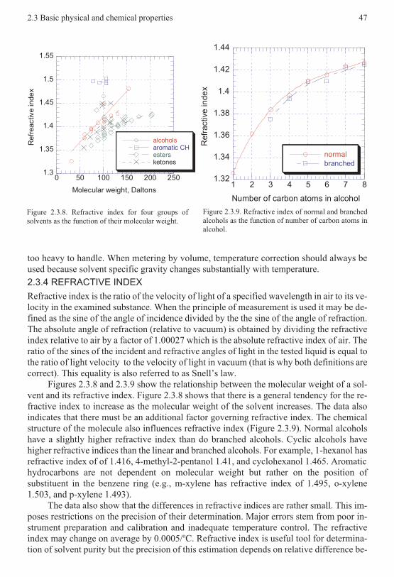
too heavy to handle. When metering by volume, temperature correction should always beused because solvent specific gravity changes substantially with temperature.

2.3.4 REFRACTIVE INDEX

Refractive index is the ratio of the velocity of light of a specified wavelength in air to its ve-locity in the examined substance. When the principle of measurement is used it may be de-fined as the sine of the angle of incidence divided by the the sine of the angle of refraction.The absolute angle of refraction (relative to vacuum) is obtained by dividing the refractiveindex relative to air by a factor of 1.00027 which is the absolute refractive index of air. Theratio of the sines of the incident and refractive angles of light in the tested liquid is equal tothe ratio of light velocity to the velocity of light in vacuum (that is why both definitions arecorrect). This equality is also referred to as Snell’s law.

Figures 2.3.8 and 2.3.9 show the relationship between the molecular weight of a sol-vent and its refractive index. Figure 2.3.8 shows that there is a general tendency for the re-fractive index to increase as the molecular weight of the solvent increases. The data alsoindicates that there must be an additional factor governing refractive index. The chemicalstructure of the molecule also influences refractive index (Figure 2.3.9). Normal alcoholshave a slightly higher refractive index than do branched alcohols. Cyclic alcohols havehigher refractive indices than the linear and branched alcohols. For example, 1-hexanol hasrefractive index of of 1.416, 4-methyl-2-pentanol 1.41, and cyclohexanol 1.465. Aromatichydrocarbons are not dependent on molecular weight but rather on the position ofsubstituent in the benzene ring (e.g., m-xylene has refractive index of 1.495, o-xylene1.503, and p-xylene 1.493).

The data also show that the differences in refractive indices are rather small. This im-poses restrictions on the precision of their determination. Major errors stem from poor in-strument preparation and calibration and inadequate temperature control. The refractiveindex may change on average by 0.0005/oC. Refractive index is useful tool for determina-tion of solvent purity but the precision of this estimation depends on relative difference be-


1.3

1.35

1.4

1.45

1.5

1.55

0 50 100 150 200 250


Refr

eactive

ind

ex

Molecular weight, Daltons

Figure 2.3.8. Refractive index for four groups ofsolvents as the function of their molecular weight.

1.32

1.34

1.36

1.38

1.4

1.42

1.44

1 2 3 4 5 6 7 8

normal

branched

Refr

active

inde

xNumber of carbon atoms in alcohol

Figure 2.3.9. Refractive index of normal and branchedalcohols as the function of number of carbon atoms inalcohol.

tween the solvent and the impurity. If this difference is small, the impurities, present insmall quantities, will have little influence on the reading.

2.3.5 VAPOR DENSITY AND PRESSURE

The relative vapor density of solvents is given by the following equation:

dM

Mvp

s

air

= [2.3.2]

where:Ms the molecular mass of solventsMair the molecular mass of air (28.95 Daltons)

Figure 2.3.10 shows that the vapor density has linear correlation with molecular mass andthat for both alcohols and ketones (as well as the other solvents) the relationship is similar.The data also show that solvent vapor densities are higher than air density. This makes ven-tilation a key factor in the removal of these vapors in the case of spill or emissions fromequipment. Otherwise, the heavier than air vapors will flow along floors and depressionsfilling pits and subfloor rooms and leading to toxic exposure and/or risk of ignition and sub-sequent explosions.

The Clausius-Clapeyron equation gives the relationship between molecular weight ofsolvent and its vapor pressure:

d p

dT

M

RT

ln = Λ2

[2.3.3]

where:p vapor pressureT temperatureM molecular mass of solventΛ heat of vaporizationR gas constant

Figure 2.3.11 shows that the vapor pressure of alcohols increases as the number of carbonatoms in the molecules and the molecular mass increases. A small increase in vapor pres-sure is produced when branched alcohols replace normal alcohols.

Vapor pressure at any given temperature can be estimated by the use of Antoine (eq.[2.3.4]) or Cox (eq. [2.3.5]) equation (or chart). Both equations are derived fromClausius-Clapeyron equation:

logp AB

C T= −

+[2.3.4]

logp AB

T= −

+ 230[2.3.5]

where:A, B, C constants. The constants A and B are different in each equation. The equations

coincide when C = 230 in the Antoine equation.

From the above equations it is obvious that vapor pressure increases with temperature.

48 George Wypych

The vapor pressure at the boiling point of a pure solvent is equal to atmospheric pres-sure. When solvents are used in mixtures or solutions, the vapor pressure is affected byother components present in the mixture. For example, if a solvent is hydrophilic, the addi-tion of a hydrophilic solute decreases the vapor pressure. The addition of a hydrophobic sol-ute to a hydrophilic solvent increases the vapor pressure. Alcohols have hydrophobicchains, therefore addition of small quantities of alcohol to water increases vapor pressure ofresulting solution. Because of these phenomena and other types of associations betweensolvents in their mixtures, theory cannot be used to accurately predict the resulting vaporpressure.

Raoult’s Law has limited prediction capability of the vapor pressure of two misciblesolvents:

p m p m p12 1 1 1 21= + −( ) [2.3.6]

where:p12 vapor pressure of the mixturem1 molar fraction of the first componentp1, p2 vapor pressures of the components

If associations exist between molecules in the mixture, the vapor pressure of the mixture islower than that predicted by the law.

2.3.6 SOLVENT VOLATILITY

The evaporation rate of solvents is important in many applications. This has resulted in at-tempts to model and predict solvent volatility. The evaporation rate of a solvent depends onits vapor pressure at the processing temperature, the boiling point, specific heat, enthalpyand heat of vaporization of the solvent, the rate of heat supply, the degree of association be-tween solvent molecules and between solvent and solute molecules, the surface tension ofthe liquid, the rate of air movement above the liquid surface, and humidity of air surround-ing the liquid surface.


1

2

3

4

5

6

20 40 60 80 100 120 140 160

alcohols

ketones

Vap

or

de

nsity

rela

tive

toair


Figure 2.3.10. Vapor density relative to air of alcoholsand ketones vs. their molecular weight.

0

20

40

60

80

100

120

140

1 2 3 4 5 6 7 8

normal

branched

Vap

or

pre

ssu

rea

t25o

C,m

mh

gNumber of carbon atoms in alcohol

Figure 2.3.11. Vapor pressure at 25oC of normal andbranched alcohols vs. number of carbon atoms in theirmolecule.

The vapor pressure of solvent was found in the previous section to depend on its mo-lecular weight and temperature. Figure 2.3.3 shows that the evaporation rate of a solventmay be predicted based on knowledge of its boiling point and Figure 2.3.4 shows that thespecific heat of solvent also relates to its boiling point. The boiling point of solvent also de-pends on its molecular weight as does enthalpy and heat of vaporization. But there is not ahigh degree of correlation among these quantities because molecular associations existwhich cannot be expressed by universal relationship. For this reason experimental valuesare used to compare properties of different solvents. The two most frequently used refer-ence solvents are: diethyl ether (Europe) and butyl acetate (USA). The evaporation rate ofother solvents is determined under identical conditions and the solvents are rankedaccordingly. If diethyl ether is used as a reference point, solvents are grouped into fourgroups: high volatility < 10, moderate volatility 10-35, low volatility 35-50, and very lowvolatility > 50. If butyl acetate is used as the reference solvent, the solvents are grouped intothree classes: rapid evaporation solvents > 3, moderate 0.8-3, and slow evaporating solvents< 0.8.

In some applications such as coatings, casting, etc., evaporation rate is not the only im-portant parameter. The composition must be adjusted to control rheological properties, pre-vent shrinkage, precipitation, formation of haze, and to provide the required morphology.Solvents with different evaporation rates can address all existing requirements.

Both the surface tension of mixture and solvent diffusion affect the evaporation rate.This becomes a complex function dependent not only on the solvents present but also on in-fluence of solutes on both surface tension and diffusion. These relationships affect the realevaporation rates of solvents from the complicated mixtures in the final products. In addi-tion, solvent evaporation also depends on relative humidity and air movement.

2.3.7 FLASH POINT

Flash point is the lowest temperature, corrected to normal atmospheric pressure (101.3kPa), at which the application of an ignition source causes the vapors of a specimen to igniteunder the specific conditions of the test. Flash point determination methods are designed tobe applied to a pure liquid but, in practice, mixtures are also evaluated. It is important to un-derstand limitations of such data. The flash point of a solvent mixture can be changed byadding various quantities of other solvents. For example, the addition of water orhalogenated hydrocarbons will generally increase the flash point temperature of mixture.The flash point can also be changed by forming an azeotropic mixture of solvents or by in-creasing the interaction between solvents. At the same time, the flash point of single compo-nent within the mixture is not changed. If conditions during production, application, or in aspill allow the separation or removal of a material added to increase the flash point, then theflash point will revert to that of the lowest boiling flammable component.

An approximate flash point can be estimated from the boiling point of solvent usingthe following equation:

Flash point = 0.74Tb[2.3.7]

Figure 2.3.5 shows that there is often good correlation between the two but there are in-stances where the relationship does not hold. The correlation for different groups of sol-vents varies between 0.89 to 0.96.

Flash point can also be estimated from vapor pressure using the following equation:

50 George Wypych

Flash point = a log p + b [2.3.8]

The constants a and b are specific to each group of solvents. Figure 2.3.12 shows that esti-mation of flash point from vapor pressure of solvent is less accurate than its estimation fromboiling point.

2.3.8 FLAMMABILITY LIMITS

Two limits of solvent flammability exist. The lower flammability limit is the minimum con-centration of solvent vapor in oxidizing gas (air) that is capable of propagating a flamethrough a homogeneous mixture of the oxidizer and the solvent vapor. Below the lowerflammability limit the mixture is too lean to burn or explode. The upper flammability limitis the maximum concentration of solvent vapor in an oxidizing gas (air) above which prop-agation of flame does not occur. Mixtures with solvent vapor concentrations above the up-per flammability limit are too rich in solvent or too lean in oxidizer to burn or explode.

The flammable limits depend on oxygen concentration, concentration of gases otherthan oxygen, the inert gas type and concentration, the size of the equipment, the direction offlame propagation, and the pressure, temperature, turbulence and composition of the mix-ture. The addition of inert gases to the atmosphere containing solvent is frequently used toreduce the probability of an explosion. It is generally assumed that if the concentration ofoxygen is below 3%, no ignition will occur. The type of inert gas is also important. Carbondioxide is more efficient inert gas than nitrogen. The size of equipment matters because ofthe uniformity of vapor concentration. A larger head space tends to increase the risk ofinhomogeneity. The cooling effect of the equipment walls influences the evaporation rateand the vapor temperature and should be used in risk assessment.

The flash point is not the temperature at which the vapor pressure in air equals thelower flammable limit. Although both parameters have some correspondence there arelarge differences between groups of solvents. There is a general tendency for solvents with alower flammability limit to have a lower flash point. The flash point determination uses a


-20

0

20

40

60

80

100

0 50 100 150 200 250

alcohols

ketones

Fla

sh

po

int,

oC

Vapor pressure, mm Hg

Figure 2.3.12. Flash point vs. vapor pressure ofsolvent.

0

1

2

3

4

5

6

7

-20 0 20 40 60 80 100 120


Lo

we

rflam

ma

bility

limit,%

Flash point,oC

Figure 2.3.13. Lower flammability limit of solvents vstheir flash points.

downward and horizontal propagation of flame. Flame propagation in these directions gen-erally requires a higher vapor concentration than it is required for the upward flame propa-gation used to determine flammability limits. The flame in flash point determination is atsome distance from the surface where the vapor concentration is at its highest (because va-pors have higher density than air) than exists on the liquid surface thus flush analysisunderestimates concentration of vapor.

An increased vapor pressure typically increases the upper limit of flammability and re-duces the lower limit of flammability. Pressures below atmospheric have little influence onflammability limits. An increase in temperature increases the evaporation rate and thus de-creases the lower limit of flammability.

There are a few general rules which help in the estimation of flammability limits. Inthe case of hydrocarbons, the lower limit can be estimated from simple formula: 6/numberof carbon atoms in molecule; for benzene and its derivatives the formula changes to: 8/num-ber of carbon atoms. To calculate the upper limits, the number of hydrogen and carbon at-oms is used in calculation.

The lower flammability limit of a mixture can be estimated from Le Chatelier’s Law:

LFL

LFL LFL LFL

mix

n

n

=+ + +

100

1

1

2

2

φ φ φL

[2.3.9]

where:φi fraction of components 1, 2, ..., nLFLi lower flammability limit of component 1, 2, ..., n

2.3.9 SOURCES OF IGNITION AND AUTOIGNITION TEMPERATURE

Sources of ignition can be divided to mechanical sources (impact, abrasive friction, bear-ings, misaligned machine parts, choking or jamming of material, drilling and other mainte-nance operations, etc), electrical (broken light, cable break, electric motor, switch gear,liquid velocity, surface or personal charge, rubbing of different materials, liquid spraying orjetting, lightning, stray currents, radio frequency), thermal (hot surface, smoking, hot trans-fer lines, electric lamps, metal welding, oxidation and chemical reactions, pilot light, arson,change of pressure, etc.), and chemical (peroxides, polymerization, catalysts, lack of inhibi-tor, heat of crystallization, thermite reaction, unstable substances, decomposition reac-tions). This long list shows that when making efforts to eliminate ignition sources, it is alsoessential to operate at safe concentrations of volatile, flammable materials because of nu-merous and highly varied sources of ignition.

The energy required for ignition is determined by the chemical structure of the sol-vent, the composition of the flammable mixture, and temperature. The energy of ignition ofhydrocarbons decreases in the order alkanes > alkenes > alkynes (the presence of double ortriple bond decreases the energy energy required for ignition). The energy requirement in-creases with an increase in molecular mass and an increase branching. Conjugated structuregenerally requires less ignition energy. Substituents increase the required ignition energy inthe following order: mercaptan < hydroxyl < chloride < amine. Ethers and ketones requirehigher ignition energy but an aromatic group has little influence. Peroxides require ex-tremely little energy to ignite.

52 George Wypych

Figure 2.3.14 shows the effect ofchanging the ratio of air to methyl ethylketone on the minimum spark ignition en-ergy. The ignition energy decreases withinthe studied range as the amount of airincreases (less flammable content). Figure2.3.15 shows the effect of temperature onthe minimum ignition energy of selectedsolvents. There are differences betweensolvents resulting from differences inchemical structure as discussed above butthe trend is consistent − a decrease of re-quired energy as temperature increases.

The autoignition temperature is theminimum temperature required to initiatecombustion in the absence of a spark orflame. The autoignition temperature de-pends on the chemical structure of solvent,

the composition of the vapor/ air mixture, the oxygen concentration, the shape and size ofthe combustion chamber, the rate and duration of heating, and on catalytic effects. Figure2.3.16 shows the effect of chemical structure on autoignition temperature. The general trendfor all groups of solvents is that the autoignition temperature decreases as molecular weightincreases. Esters and ketones behave almost identically in this respect and aromatic hydro-carbons are very similar. The presence of a hydroxyl group substantially reducesautoignition temperature.


0.2

0.6

1

1.4

0.9 1.1 1.3 1.5 1.7

Min

imu

msp

ark

ign

itio

ne

ne

rgy,m

J

Stoichiometric air to solvent ratio

Figure 2.3.14. Minimum ignition energy vs.stoichiometric ratio of air to methyl ethyl ketone.[Data from H F Calcote, C A Gregory, C M Barnett,R B Gilmer, Ind. Eng. Chem., 44, 2656 (1952)].

0.1

0.2

0.3

0.4

20 60 100 140

ethyl acetatetolueneethanol

Min

imu

mig

nitio

ne

ne

rgy,

mJ

Temperature,oC

Figure 2.3.15. Minimum ignition energy vs.temperature for selected solvents. [Data fromV S Kravchenko, V A Bondar, Explosion Safety ofelectrical Discharges and Frictional Sparks,Khimia, Moscow, 1976].

250

300

350

400

450

500

20 40 60 80 100 120 140 160


Auto

ignitio

nte

mpe

ratu

re,o

C


Figure 2.3.16. Autoignition temperature of selectedsolvents vs. their molecular weight.

The effect of the air to solvent ratio onautoignition temperature is similar to thaton ignition energy (see Figure 2.3.14). Asthe oxygen concentration increases withinthe range of the flammability limits, theautoignition temperature increases. Theautoignition temperature increases whenthe size of combustion chamber decreases.Rapid heating reduces the autoignitiontemperature and catalytic substance maydrastically reduce it.

2.3.10 HEAT OF COMBUSTION(CALORIFIC VALUE)

Heat of combustion, also known as calo-rific value, is the quantity of energy permole released during combustion. It coin-cides with the heat of reaction. Solventshave higher heats of combustion than typi-

cal fuels such as natural gas, propane or butane. They can be very good source of energy inplants which process solutions. In addition to supplying energy, the combustion of solventscan be developed to be one of the cleanest method of processing from solutions. Twoapproaches are commonly used: solvent vapors are directed to a combustion chamber orspent solvents are burned in furnaces. The heat of combustion of a liquid solvent is less than1% lower than the heat of combustion of a vapor.

Figure 2.3.17 shows the relationship between the heat of combustion and the numbernumber of carbon atoms in the molecule. The heat of combustion increases as molecularweight increases and decreases when functional groups are present.

2.3.11 HEAT OF FUSION

Heat of fusion is the amount of heat to melt the frozen solvent. It can be used to determinethe freezing point depression of solute.

2.3.12 ELECTRIC CONDUCTIVITY

Electric conductivity is the reciprocal of specific resistance. The units typically used are ei-ther ohm-1 m-1 or, because the conductivities of solvents are very small picosiemens per me-ter which is equivalent to10-12 ohm-1 m-1. The electric conductivity of solvents is very low(typically between 10-3 - 10-9 ohm-1 m-1). The presence of acids, bases, salts, and dissolvedcarbon dioxide might contribute to increased conductivity. Free ions are solely responsiblefor the electric conductivity of solution. This can be conveniently determined by measuringthe conductivity of the solvent or the conductivity of the water extract of solvent impurities.The electronic industry and aviation industry have the major interest in these determina-tions.

2.3.13 DIELECTRIC CONSTANT (RELATIVE PERMITTIVITY)

The dielectric constant (or relative permittivity) of a solvent reflects its molecular symme-try. The value of the dielectric constant is established from a measurement relative to vac-uum. The effect is produced by the orientation of dipoles along an externally applied

54 George Wypych

0

1000

2000

3000

4000

5000

6000

1 2 3 4 5 6 7 8

n-hydrocarbons

alcohols

He

at

of

co

mb

ustio

n,kJ

mo

l-1

Number of carbon atoms

Figure 2.3.17. Heat of combustion vs. number of carbonatoms in molecule.

electric field and from the separation of charges in apolar molecules. This orientation causespolarization of the molecules and a drop in electric field strength. Dielectric constant datamay be used in many ways. In particular, it is the factor which permits the evaluation ofelectrostatic hazards. The rate of charge decay is a product of dielectric constant and resis-tivity.

In solvent research, dielectric constant has a special place as a parameter characteristicof solvent polarity. The dielectric constant, ε, is used to calculate dipole moment, µ:

µ εε

= −−

1

2VM

[2.3.10]

where:VM molar volume

The product of dipole moment and dielectric constant is called the electrostatic factor and itis a means of classifying solvents according to their polarity.

Figure 2.3.18 shows that the dielectric constant correlates with molecular weight. It isonly with aliphatic hydrocarbons that the dielectric constant increases slightly as the molec-ular weight increases. The dielectric constant of alcohols, esters, and ketones decreases astheir molecular weight increases, but only alcohols and ketones have the same relationship.The dielectric constants of esters are well below those of alcohols and ketones.

The dielectric constant also correlates with refractive index. In the case of aliphatichydrocarbons, the dielectric constant increases slightly as refractive index increases. Botharomatic and aliphatic hydrocarbons have dielectric constants which follow the relation-ship: ε ≈ n D

2 . The dielectric constants of alcohols, esters and ketones decrease as the refrac-tive constants increase but only alcohols and ketones form a similar relationship. Thedielectric constants of ketones poorly correlate with their refractive indices.


0

5

10

15

20

25

30

35

20 40 60 80 100 120 140

alcoholsaliphatic CHestersketones

Die

lectr

iccon

sta

nt


Figure 2.3.18. Dielectric constant vs. molecularweight of selected solvents.

0

5

10

15

20

25

30

35

1.3 1.35 1.4 1.45 1.5

alcoholsaliphatic CHestersketones

Die

lectr

iccon

sta

nt

Refractive index

Figure 2.3.19. Dielectric constant of selected solventsvs. their refractive index.

2.3.14 OCCUPATIONAL EXPOSURE INDICATORS

The measurement of solvent concentration in the workplace place is required by nationalregulations. These regulations specify, for individual solvents, at least three different con-centrations points: the maximum allowable concentration for an 8 hour day exposure, themaximum concentration for short exposure (either 15 or 30 min), and concentration whichmust not be exceeded at any time. These are listed in the regulations for solvents. The listingis frequently reviewed and updated by the authorities based on the most currently availableinformation.

In the USA, the threshold limit value, time-weighted average concentration,TLV-TWA, is specified by several bodies, including the American Conference of Govern-mental Industrial Hygienists, ACGIH, the National Institute of Safety and Health, NIOSH,and the Occupational Safety and Health Administration, OSHA. The values for individualsolvents stated on these three lists are very similar. Usually the NIOSH TLV-TWA arelower than on the other two lists. Similar specifications are available in other countries (forexample, OES in UK, or MAK in Germany). The values for individual solvents are selectedbased on the presumption that the maximum allowable concentration should not causeinjury to a person working under these conditions for 8 hours a day.

For solvent mixtures, the following equation is used in Germany to calculate allow-able limit:

Ic

MAKMAK

i

ii

i n

==

=

∑1

[2.3.11]

where:IMAK evaluation indexc concentrations of components 1, 2, ..., nMAK maximum permissible concentrations for components 1, 2, ..., n

The maximum concentrations for short exposure is the most frequently limit specifiedfor an exposure of 15 min with a maximum of 4 such occurrences per day each occurring atleast 60 min apart from each other. These values are 0-4 times larger than TLVs. They areselected based on the risks associated with an individual solvent.

Solvent concentrations which should not be exceeded at any time are seldom specifiedin regulations but, if they are, the values stated as limits are similar to those on the three lists.

In addition, to maintaining concentration below limiting values, adequate protectionshould be used to prevent the inhalation of vapors and contact with the skin (see Chapter24).

2.3.15 ODOR THRESHOLD

The principal for odor threshold was developed to relate the human sense of smell to theconcentration of the offending substances. If the substance is toxic, its detection may pro-vide early warning to the danger. However, if the odor threshold is higher than the concen-tration at which harm may be caused it is not an effective warning system. Toxic substancesmay have very little or no odor (e.g., carbon monoxide) and an individual’s sense of smellmay vary widely in its detection capabilities. A knowledge of odor threshold is most usefulin determining the relative nuisance factor for an air pollutant when designing a control sys-tem to avoid complaints from neighboring people surrounding a facility. Regulations oftenstate (as they do for example in Ontario, Canada) that, even when the established concentra-

56 George Wypych

tion limits for air pollutants are met, if neighbors complain, penalties will be applied. Figure2.3.6 shows that odor threshold is related to the boiling point (although odor threshold de-creases with boiling point increasing). It is known from comparisons of TLV and odor de-tection that odor detection is not a reliable factor.

2.3.16 TOXICITY INDICATORS

Lethal dose, LD50, and lethal concentration, LC50, are commonly used indicators of sub-stance toxicity. LD50 is reported in milligrams of substance per kilogram of body weight tocause death in 50% of tested animals (exception is LC50 which is given in ppm over usuallythe period of 4 hours to produce the same effect). It is customary to use three values:LD50-oral, LD50-dermal, and LC50-inhalation which determine the effect of a chemicalsubstance on ingestion, contact with the skin and inhalation. The preferred test animal forLD50-oral and LC50-inhalation is the rat. The rabbit is commonly used for LD50-dermaldetermination but other test animals are also used.

There is no official guideline on how to use this data but the Hodge-Sterner table is fre-quently referred to in order to assign a particular substance to a group which falls within cer-tain limits of toxicity. According to this table, dangerously toxic substances are those whichhave LD50 < 1 mg/kg, seriously toxic - 1-50, highly toxic - 50-500, moderately toxic -500-5,000, slightly toxic - 5,000-15,000, and extremely low toxic - >15,000 mg/kg. Usingthis classification one may assess the degree of toxicity of solvents based on a lethal dosescale. No solvent is classified as a dangerously toxic material. Ethylenediaminetetraaceticacid and furfural are seriously toxic materials. Butoxyethanol, ethylene oxide, formalde-hyde, metasulfonic acid, 3-methyl-2-butanone, N-nitrosodimethylamine, and triethylamineare classified as highly toxic material. The remaining solvents fall into the moderately,slightly, and extremely low toxic material classes.

The LD50-oral is usually assigned a lower value than LD50-dermal but there are manycases where the opposite applies. Toxicity information is usually further expanded by add-ing more details regarding test animals and target organs.

In addition to estimates of toxicity for individual solvents, there are lists whichdesignate individual solvents as carcinogenic, mutagenic, and reproductively toxic. Theselists contain the name of solvent with yes or no remark (or similar). If a solvent is not presenton the list that does not endorse its benign nature because only materials that have beentested are included in the lists. To further elaborate, materials are usually divided into threecategories: substance known to cause effect on humans, substance which has causedresponses in animal testing and given reasons to believe that similar reactions can be ex-pected with human exposures, and substance which is suspected to cause responses basedon experimental evidence.

In the USA, four agencies generate lists of carcinogens. These are: the EnvironmentalProtection Agency, EPA, the International Agency for Research on Cancer, IRAC, the Na-tional Toxicology Program, NTP, and the Occupational Safety and Health Administration,OSHA. Although, there is a good agreement between all four lists, each assessment differsin some responds. The following solvents made at least one of the lists (no distinction isgiven here to the category assignment but any known or suspected carcinogen found on anylist is given (for more details see Chapter 3)): acetone, acrolein, benzene, carbon tetrachlo-ride, dichloromethane, 1,4-dioxane, ethylene oxide, formaldehyde, furfural, d-limonene,N-nitrosodimethyl amine, propylene oxide, tetrachloroethylene, 2,4-toluenediisocyanate,1,1,2-trichloroethylene, and trichloromethane.


Mutagenic substances have the ability to induce genetic changes in DNA. Themutagenicity list maintained in the USA includes the following solvents: all solvents listedabove for carcinogenic properties with exception of dichloromethane, d-limonene, andtetrachloroethylene. In addition, the following long list solvents: 1-butanol, 2-butanol,γ-butyrolactone, 2-(2-n-butoxyethoxy)ethanol, chlororodifluoromethane, chloromethane,diacetone alcohol, dichloromethane, diethyl ether, dimethyl amine, dimethylene glycoldimethyl ether, dimethyl sulfoxide, ethanol, 2- ethoxyethanol, 2-ethoxyethanol acetate,ethyl acetate, ethyl propionate, ethylbenzene, ethylene glycol diethyl ether, ethylene glycolmethyl ether acetate, ethylene glycol monophenyl ether, ethylenediaminetetraacetic acid,formic acid, furfuryl alcohol, heptane, hexane, methyl acetate, 3-methyl-2-butanol, methylester of butyric acid, methyl propionate, N-methylpyrrolidone, monomethylamine,1-octanol, 1-pentanol, 1-propanol, propyl acetate, sulfolane, 1,1,1-trichloroethane,triethylene glycol, triethylene glycol dimethyl ether, trifluoromethane, trimethylene glycol,and xylene (mixture only). It is apparent that this much longer list includes commonly usedsolvents from the groups of alcohols, halogenated solvents, hydrocarbons, glycols, and es-ters.

The following solvents are reported to impair fertility: chloroform, ethylene glycoland its acetate, 2-methoxypropanol, 2-methoxypropyl acetate, dichloromethane, methyleneglycol and its acetate, and N,N-dimethylformamide.

2.3.17 OZONE - DEPLETION AND CREATION POTENTIAL

Ozone depletion potential is measured relative to CFC-11 and it represents the amount ofozone destroyed by emission of a vapor over its entire atmospheric lifetime relative to thatcaused by the emission of the same mass of CFC-11.

Urban ozone formation potential is expressed relative to ethene. It represents the po-tential of an organic solvents vapor to form ozone relative to that of ethene ((g O3/g sol-vent)/(g O3/g ethene)). Several groups of solvents, including alcohols, aldehydes, amines,aliphatic and aromatic hydrocarbons, esters, ethers, and ketones are active in ozoneformation. Aldehydes, xylenes, some unsaturated compounds, and some terpenes are themost active among those.

2.3.18 OXYGEN DEMAND

There are several indicators of solvent biodegradation. Most solvents have a biodegradationhalf-life of days to weeks and some biodegrade even faster.

The amount of oxygen required for its biodegradation is a measure of a solvent’s im-pact on natural resources. Several factors are used to estimate this, such as biological oxy-gen demand, BOD, after 5-day and 20-day aerobic tests, chemical oxygen demand, COD,and theoretical oxygen demand, TOD. All results are given in grams of oxygen per gram ofsolvent. COD is the amount of oxygen removed during oxidation in the presence of per-manganate or dichromate. TOD is the theoretically calculated amount of oxygen required tooxidize solvent to CO2 and H2O. Most alcohols and aromatic hydrocarbons have a highestBOD5. They consume twice their own weight in oxygen.

2.3.19 SOLUBILITY

The prediction of solubility of various solutes in various solvents is a major focus of re-search. An early theory has been that “like dissolves like”. Regardless of the apparent meritsof this theory it is not sufficiently rigorous and is overly simple.

58 George Wypych

A universal approach was developed by Hildebrand who assumed that the mutual sol-ubility of components depends on the cohesive pressure, c. The square root of cohesivepressure is the Hildebrand’s solubility parameter, δ:

δ = =−

cH RT

V

v

m

∆[2.3.12]

where:∆Hv heat of vaporizationR gas constantT temperatureVm molar volume of solvent = M/dM molecular mass of solventd density of solvent

Frequently, the term RT is neglected because it accounts for only 5-10% of the heat ofvaporization. This equation explains the reasons for the correlation between the Hildebrandsolubility parameter and heat of vaporization as given in Figure 2.3.1.

The Hildebrand model takes into account only the dimensions of molecules or of themolecular segments participating in the process of solvation and dispersion interactions.The model is useful, therefore, in predicting the solubility of non-polar substrates. The solu-bility parameters of solvents and solutes are compared and if they are similar there is highprobability (exceptions exist) that the solvents are miscible that a solute is soluble in a sol-vent. Two solvents having the same solubility parameters should have the same dissolvingcapabilities. If one solvent has solubility parameter slightly below the solubility parameterof solute and the second solvent has solubility parameter above the solute, the mixture ofboth solvents should give better results than either solvent alone. This model is an experi-mental and mathematical development of the simple rule of “like dissolves like”.

Solvents and solutes also interact by donor-aceptor, electron pair, and hydrogen bond-ing interactions. It can be predicted that the above concept is not fully universal, especiallyin the case of solutes and solvents which may apply these interactions in their solubilizingaction. Hansen developed a three-dimensional scale with parameters to expand theory in or-der to include these interactions. Hansen defined solubility parameter by the followingequation:

δ δ δ δ2 2 2 2= + +d p h[2.3.13]

where:δd dispersion contribution to solubility parameterδp polar contribution to solubility parameterδh hydrogen bonding contribution to solubility parameter

Hansen defined solvent as a point in three-dimensional space and solutes as volumes(or spheres of solubility). If a solvent point is within the boundaries of a solute volume spacethen the solute can be dissolved by the solvent. If the point characterizing the solvent isoutside the volume space of a solute (or resin) such a solvent does not dissolve the solute.The solubility model based on this concept is broadly applied today by modern computertechniques using data obtained for solvents (the three components of solubility parameters)and solutes (characteristic volumes). A triangular graph can be used to outline the limits of


solubility and place different solvents within the matrix to determine their potential dissolv-ing capability for a particular resin.

Simpler methods are also used. In the paint industry, Kauri butanol values are deter-mined by establishing the tolerance of a standard solution of Kauri resin in n-butanol to theaddition of diluents. This method is applicable to hydrocarbons (both aromatic andaliphatic) and CFCs. Figure 2.3.20 shows that there is a good correlation between the Kauributanol number and the Hildebrand solubility parameter. The Kauri butanol number can beas high as 1000 (amyl ester of lactic acid) or 500 (Freon solvent M-162).

The aniline point determination is another method of establishing the solubilizingpower of a solvent by simple means. Here, the temperature is measured at which a solutionjust becomes cloudy. Figure 2.3.21 shows that there is a good correlation between the Kaurinumber and the aniline point. Also dilution ratio of cellulose solution is measured by stan-dardized methods (see Chapter 15).

2.3.20 OTHER TYPICAL SOLVENT PROPERTIES AND INDICATORS

There are many other solvent properties and indices which assist in solvent identificationand selection and help us to understand the performance characteristics of solvents. Mostdata characterizing the most important properties were discussed in the sections above. Thesolvent properties and classification indicators, which are discussed below, are included inthe Solvent Database available on CD-ROM from ChemTec Publishing.

Name. A solvent may have several names such as common name, Chemical Abstractsname, and name according to IUPAC systematic nomenclature. Common names have beenused throughout this book and in the CD-ROM database because they are well understoodby potential users. Also, CAS numbers are given in the database to allow user of the data-base to use the information with Chemical Abstract searches. In the case of commercial sol-vents which are proprietary mixtures, the commercial name is used.

The molecular formula for each solvent is given in the database, followed by the mo-lecular formula in Hills notation, and the molecular mass (if solvent is not a mixture).

60 George Wypych

20

40

60

80

100

120

140

7 7.5 8 8.5 9 9.5 10

aliphatic CHaromatic CHCFC

R2= 0.994

R2= 0.996

R2= 0.992

Kau

rib

uta

no

lnu

mb

er

Hildebrand solubility parameter, cal-1/2

cm-3/2

Figure 2.3.20. Kauri butanol number vs. Hildebrandsolubility parameter.

25

30

35

40

45

50

55

10 20 30 40 50 60 70 80

y = 62.2 - 0.47x R2= 0.996

Kau

rib

uta

no

lnu

mb

er

Aniline point,oC

Figure 2.3.21. Kauri butanol number vs. aniline point.

The CAS number identifies thechemical compound or composition with-out ambiguity.

RTECS number is the symbol givenby Registry of Toxic Effects of ChemicalSubstances (e.g. AH4025000) to identifytoxic substances.

Composition is given for solventswhich are manufactured under trade nameand have a proprietary composition (if suchinformation is available).

Solvent purity (impurities) is givenas a percent and known impurities and theirconcentrations are provided.

Hygroscopicity and water solubilityof solvents is an important characteristic inmany applications. The data are given inthe database either in mg of water per kilo-

gram of solvent or in a generic statement (e.g. miscible, slight). Many solvents are hygro-scopic, especially those which contain hydroxyl groups. These solvents will absorb waterfrom their surrounding until equilibrium is reached. The equilibrium concentration dependson the relative humidity of air and the temperature. If solvents must maintain a low concen-tration of water, vents of storage tanks should be fitted with silica gel or molecular sievescartridges or tanks should be sealed and equipped with pressure and vacuum relief ventswhich open only to relieve pressure or to admit a dry inert gas to replace the volume pumpedout. Preferably prevention of water from contacting solvents or the selection of solventswith a low water content is more economical than the expensive operation of drying a wetsolvent.

Surface tension and solubility parameter have been related in the following equation:

δ γ=

211 3

./

KV

a

[2.3.14]

where:δ Hildebrand solubility parameterK, a constantsγ surface tensionV molar volume of the solvent

However, Figure 2.3.22 shows that the parameters correlate only for aromatic hydrocar-bons. For three other groups the points are scattered. The equation has a very limited predic-tive value.

Viscosity. Figure 2.3.2 shows that viscosity of solvents correlates with their boilingpoint. There are substantial differences in the viscosity - boiling point relationship amongalcohols and other groups of solvents. These are due to the influence of hydrogen bondingon the viscosity of alcohols.


7

8

9

10

11

12

13

14

15

20 25 30 35 40 45


Hild

eb

ran

dso

lubility

pa

ram

ete

r,cal1/2

cm

-3/2

Surface tension, dynes cm-2

Figure 2.3.22. Hildebrand solubility parameter vs.surface tension for four groups of solvents.

Thermal conductivity of solvents is an important property which determines the heattransfer in a solvent or solution and influences the evaporation rate of solvents as a solutionis being dried.

Activity coefficients may be applied to different processes. In one application, the ac-tivity coefficient is a measure of the escaping tendency from liquid to another liquid or agaseous phase (in the liquid to gas phase they can be quantified using Henry’s Law coeffi-cient). These activity coefficients are derived from distillation data at temperatures near theboiling point or from liquid-liquid extraction calculations. In another application as definedby Hildebrand and Scratchard solvent activity to dissolve a non-electrolyte solute is givenby equation:

( )lnf

V

RT

m solute sovent=−δ δ 2

[2.3.15]

where:f activity coefficientVm molar volume of soluteδsolute solubility parameter of soluteδsolvent solubility parameter of solventRT gas constant x temperature

This coefficient is used to express rate constants of bimolecular reactions.Azeotropes. One solvent may form azeotropes with another solvent due to molecular

association. This physical principle can be exploited in several ways. The most important insolvent applications is the possibility of reducing the boiling temperature (some azeotropeshave lower boiling point) therefore an applied product such as a coating may lose its sol-vents and dry faster. The formation of such azeotrope also lowers flash point by which it in-creases hazards in product use. The formation of an azeotrope is frequently used to removewater from a material or a solvent. It affects the results of a distillation since azeotrope for-mation makes it difficult to obtain pure components from a mixture by distillation.Azeotrope formation can be suppressed by lowering the boiling point (distillation undervacuum). One benefit of azeotropic distillation is the reduction in the heat required to evap-orate solvents.

Henry’s constant is a measure of the escaping tendency of a solvent from a very di-lute solution. It is given by a simple equation: Henry’s constant = p × φ, where p is the pres-sure of pure solvent at the solution temperature and φis the solvent concentration in theliquid phase. A high value of Henry’s constant indicates that solvent can be easily strippedfrom dilute water solution. It can also be used to calculate TLV levels by knowing concen-tration of a solvent in a solution according to the equation: TLV (in ppm) = [18 H (concen-tration of solvent in water)]/ molecular weight of solvent.

pH and corrosivity. The pH of solvents is of limited value but it is sometimes useful ifthe solvent has strong basic or acidic properties which could cause corrosion problems.

The acid dissociation constant is the equilibrium constant for ionization of an acidand is expressed in negative log units.

The color of a solvent may influence the effect of solvent on the final product and al-low the evaluation of solvent quality. The colorless solvents are most common but there aremany examples of intrinsically colored solvents and solvents which are colored because ofan admixture or inadequate storage conditions or too long storage.

62 George Wypych

Odor. Odor threshold (discussed above) is not a precise tool for estimation concentra-tion of vapors. The description of odor has little relevance to the identification of solvent butdescription of odors in the database may be helpful in the selection of solvent to minimizeodor or make it less intrusive.

UV absorption maxima for different solvents given in the database are useful to pre-dict the potential effect of solvent on UV absorption from sun light. The collection of data isalso useful for analytical purposes.

Solvent partition - activated carbon and between octanol and water. Solvents canbe economically removed from dilute solutions by activated carbon or ion exchange resins.Activated carbon partition coefficient which helps to determine the amount of activated car-bon needed to remove a contaminant can be obtained using the following equation:

mw

Pc= [2.3.16]

where:w total weight of solvent in solutionP partition coefficientc residual concentration of solvent remaining after treatment.

The octanol/water partition coefficient is the log of solubility of the solvent in waterrelative to that in octanol. This coefficient is used to estimate biological effects of solvents.It can also be used to estimate the potential usefulness of a solvent extraction from water byany third solvent.

Soil adsorption constant is a log of the amount of a solvent absorbed per unit weightof organic carbon in soil or sediment.

Atmospheric half-life of solvents due to reaction in the atmosphere with hydroxylradicals and ozone is a measure of the persistence of particular solvent and its effect on at-mospheric pollution.

Hydroxyl rate constant is the reaction rate constant of the solvent with hydroxyl radi-cals in the atmosphere.

Global warming potential of a well-mixed gas is defined as the time-integrated com-mitment to radiative forcing from the instantaneous release of 1 kg of trace gas expressedrelative to that from the release of 1 kg of CO2.

Biodegradation half-life determines persistence of the solvent in soil. Commercialproprietary solvents mixtures are classified as biodegradable and solvents having knownchemical compositions are classified according to the time required for biodegradation tocut their initial mass to half.

Target organs most likely affected organs by exposure to solvents. The databasecontains a list of organs targeted by individual solvents.

Hazchem Code was developed in the UK for use by emergency services to determineappropriate actions when dealing with transportation emergencies. It is also a useful to ap-ply as a label on storage tanks. It consists a number and one or two letters. The numberinforms about the firefighting medium to be used. The first letter gives information on ex-plosion risk, personal protection and action. A second letter (E) may be added if evacuationis required.


Fundamental Principles Governing Solvents...

Documents

Transcript of Fundamental Principles Governing Solvents...