Fundamental Principles and Results of a New Astronomic Theory … › images › PaperPDF ›...

Fundamental Principles and Results of a New Astronomic Theory of Climate Change

Joseph J. Smulsky

Institute of Earth’s Cryosphere, Malygina Str. 86, PO Box 1230, Tyumen, 625000, Russia Email: [email protected]

Abstract. In light of the latest research developments, this paper describes the fundamental principles of the astronomic theory of climate change. It comprises three problems: the evolution of the orbital motion, the evolution of the Earth’s rotational motion and the evolution of the insolation controlled by the evolutions of those motions. All the problems have been solved in a new way and other methods. The paper demonstrates geometric parameters of the Earth’s insolation by the Sun, and explains a new insolation theory. Its results are identical to the results of the previous theory. The equations of orbital movement are established, is told about their solution and the results for the different periods of time are submitted. These results improve the results of the previous theories: the planets’ and the Moon’s orbits are stable and the Solar system is stable. In much the same way, the problem of the Earth’s rotation is described. Unlike the previous papers, this problem is solved here without simplification. The calculations demonstrate significant oscillation of the Earth’s axis. These results were confirmed with other three independent solutions of the Earth’s rotation problem. The oscillations of the Earth’s axis result in such oscillations of insolation that explain the paleoclimate changes. The material in this paper is presented in a format intelligible for a broad audience.

Keywords: Evolution, Earth’s orbit, rotational axes, insolation, cause, climate, change.

1 Introduction

The Earth’s history is marked by numerous iterations of warm and cold spells [1]-[2]. A glacier that used to cover the north and midland of Europe melted ten thousand years ago. On the other hand, polar areas that are now almost inanimate used to be covered by rich vegetation with trees, as well as populated by abundant fauna, such as mammoths, wooly rhinoceroses, buffalos, horses and other animals. What is the reason for this sort of climate fluctuations on the Earth?

Back in the 19th century, Louis Agassiz [3], J. Adhemar [4], James Croll [5] and others fathered the idea that changes of the Earth’s orbit parameters and its rotation axis may entail change in the amount of heat reaching the Earth’s surface from the Sun in different latitudes. By the end of the 19th century, accomplishments in mathematical astronomy enabled the scientists to calculate changes of orbital and rotational parameters of the Earth, and in the beginning of the 20th century Milutin Milankovitch [6] completed work on his Astronomical Theory of Ice Ages, which is, in essence, an astronomical theory of climate change. In this theory, Milankovitch calculates the Earth’s insolation in different latitudes based on three parameters: eccentricity e of the Earth’s orbit, perihelion angular position φpγ and obliquity .

Radiation of the Earth by the Sun and the value of resulting heat on the surface is commonly known as insolation (in-sol, where in is a verb prefix with a meaning of “bring”, “lead”, and solis is sun). At the same time, we must bear in mind that the same process has other aspects denoted by different terms, such as irradiation, illumination, radiation, etc. Insolation may be expressed for different time periods, including momentary, daily, seasonal, half-year, or yearly insolation.

Inasmuch as parameters e, φpγ and change and fluctuate within periods of tens of thousands of years, insolation values from age to age may be calculated, for example, for the warm half-year period at the latitude of 65°, and the change of insulation values may lead to certain conclusions on climate change. However, the fluctuation amplitude for eccentricity e and obliquity in the Milankovitch theory was fairly small. For example, the angle fluctuated within the range of ± 1°. Such oscillations could result in temperature fluctuations also in the range of 1-2°C. This is why the astronomical theory of

Advances in Astrophysics, Vol. 1, No. 1, May 2016 https://dx.doi.org/10.22606/adap.2016.11001 1

Copyright © 2016 Isaac Scientific Publishing AdAp

climate change has caused doubt among the researchers [7] of paleoclimate both at the times of Milankovitch and today.

After M. Milankovitch, his research was repeated by several groups of researchers [8]-[13] at intervals of several decades. They updated the evolution of parameters e, φpγ and and extended the initial calculation for the past 600 thousand years [6] over a longer period, such as 30 million years [10]. Still, the main result, i.e. oscillation of eccentricity e and obliquity , remained fairly insignificant.

It was found in the second half of the 20th century that marine sediments demonstrate oscillations of the quantity of oxygen isotope O18. Vast research was carried out all across the global ocean. Results of this research were summarized in the form of standard relations of relative oxygen isotope concentration

Oδ 18 versus sediment thickness associated with time T [14]. These relations were named using initial letters of CLIMAP [16] project or names of the authors of LR-4 [15]. It is believed that lighter isotope O16 contained in the water evaporates and accumulates in glaciers. In this context, it was assumed that surplus of oxygen isotope O18, i.e. excess of Oδ 18 above the mean level, is proportionate to the volume of ice accumulated in the Earth’s ice cover.

One of the major periods on the Oδ 18 curve is 100 million years. It is close to one of the periods of change in the Earth’s orbit eccentricity e. Therefore, it was identified that eccentricity e has a significant impact on the Earth’s climate. For example, study [7] even claims that M. Milankovitch does not take into account the direct impact of eccentricity on the Earth’s climate. In fact, the insolation theory that was developed by Milankovitch identifies a mathematically strict dependence of insolation on parameters e, φpγ and [17]. On the other hand, a lot more has to be done to determine the developments and causes of establishment of certain properties of marine sediments, glacial cores of contemporary glaciers, and other paleoclimatic data arrays. The same work has to be done to identify reliability of findings offered by the astronomical climate theory. This is what we have been working on at the Institute of the Earth Cryosphere for the past two decades.

Astronomical climate theory is based on the computation of body interactions. For that reason, to make sure our findings are valid, we studied the fundamentals of mechanics, tried to remove the odd stuff and keep what is necessary [18]. The astronomical theory of the Earth’s climate includes such elements as the problems of orbital motion of bodies and rotational motion of the Earth, as well as the problem of the Earth’s insolation as function of the parameters of its orbital and rotational motions.

We mentioned above that several generations of researchers consistently repeated the studies of M. Milankovitch. Still, they all followed the same path that had been developed in mathematical astronomy over centuries. We take a different path. We do not copy equations of our predecessors but derive them on the basis of fundamental principles. Second, we seek to employ minimum simplification in our derivations. And third, we solve problems using numerical procedures, aiming to employ their most accurate variations or create new ones. In this study, the Astronomical theory of the climate change is presented in the results that we have obtained. In the beginning, we will speak about insolation of the Earth, and then about the evolution of the orbital motion and evolution of the Earth’s axis. As regards the first two problems, our independent studies confirm findings of our predecessors, while the results of the rotational motion study are different. The oscillation amplitude of obliquity is seven times greater than the value identified by pervious theories. These oscillations result in such fluctuations of insolation that can explain the past climate changes. This significant difference in the results of the Earth rotation problem requires a comprehensive verification. The final part of this study will focus on the verification of solutions of the Earth rotation problem.

2 Geometric Characteristics of Insolation

Let us place observer M in the center of celestial sphere 1 (see Fig. 1). Its horizon crosses the celestial sphere in circle HH. A perpendicular to the plane of the horizon crosses the celestial sphere at the point of zenith Z. The Earth’s axis of rotation marked by the Earth’s angular velocity vector E

crosses the celestial sphere at the point of the north pole N. Angle formed by E

and the plane of horizon represents the observer’s latitude. Bear in mind that the angle of arc of the sphere’s great circle is equal to the central angle between the radii of its ends, e.g., arc φ equals HMN.

Annual movement of the Sun S projects onto the celestial sphere 1 an ecliptic circle EE in counter-clockwise direction. This elliptic circle intersects the equator circle AA in points γ and ’γ . Longitude

2 Advances in Astrophysics, Vol. 1, No. 1, May 2016

AdAp Copyright © 2016 Isaac Scientific Publishing

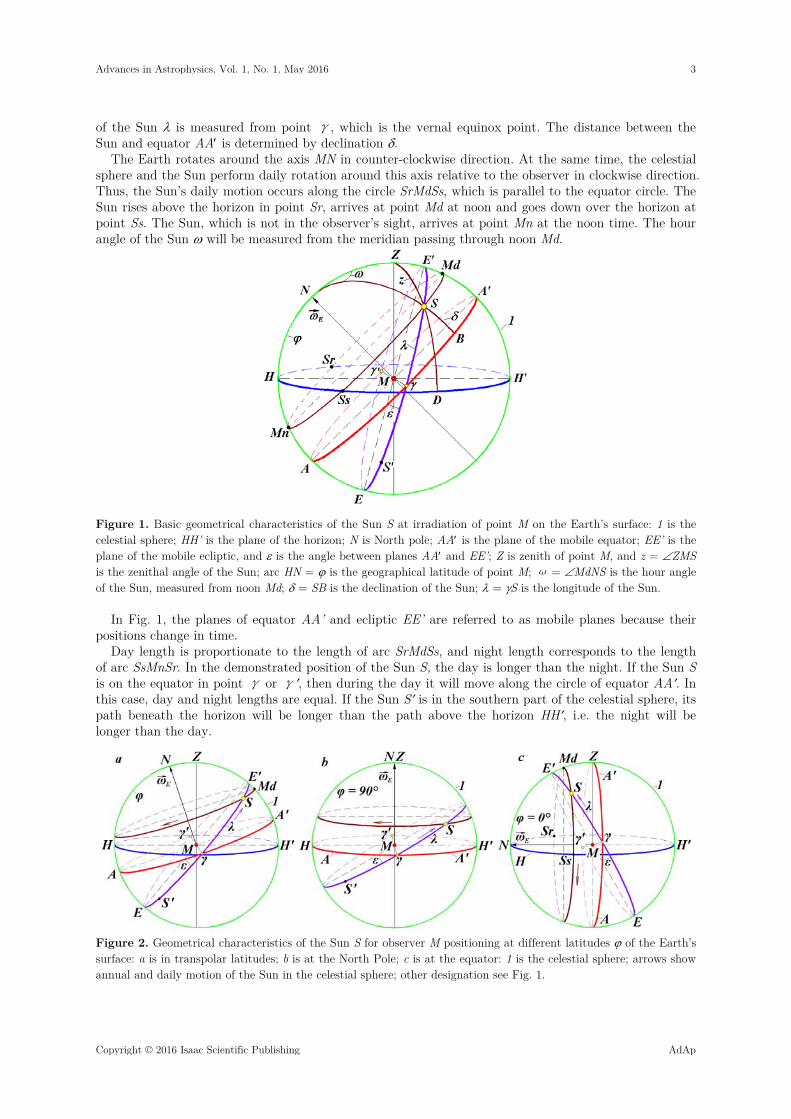
of the Sun is measured from point γ, which is the vernal equinox point. The distance between the Sun and equator AA is determined by declination .

The Earth rotates around the axis MN in counter-clockwise direction. At the same time, the celestial sphere and the Sun perform daily rotation around this axis relative to the observer in clockwise direction. Thus, the Sun’s daily motion occurs along the circle SrMdSs, which is parallel to the equator circle. The Sun rises above the horizon in point Sr, arrives at point Md at noon and goes down over the horizon at point Ss. The Sun, which is not in the observer’s sight, arrives at point Mn at the noon time. The hour angle of the Sun will be measured from the meridian passing through noon Md.

Figure 1. Basic geometrical characteristics of the Sun S at irradiation of point M on the Earth’s surface: 1 is the celestial sphere; HH’ is the plane of the horizon; N is North pole; AA is the plane of the mobile equator; EE’ is the plane of the mobile ecliptic, and is the angle between planes AA and EE’; Z is zenith of point M, and z = ZMS is the zenithal angle of the Sun; arc HN = is the geographical latitude of point M; ω = MdNS is the hour angle of the Sun, measured from noon Md; = SB is the declination of the Sun; = S is the longitude of the Sun.

In Fig. 1, the planes of equator AA’ and ecliptic EE’ are referred to as mobile planes because their positions change in time.

Day length is proportionate to the length of arc SrMdSs, and night length corresponds to the length of arc SsMnSr. In the demonstrated position of the Sun S, the day is longer than the night. If the Sun S is on the equator in point γ or γ, then during the day it will move along the circle of equator AA. In this case, day and night lengths are equal. If the Sun S is in the southern part of the celestial sphere, its path beneath the horizon will be longer than the path above the horizon HH, i.e. the night will be longer than the day.

Figure 2. Geometrical characteristics of the Sun S for observer M positioning at different latitudes of the Earth’s surface: a is in transpolar latitudes; b is at the North Pole; c is at the equator: 1 is the celestial sphere; arrows show annual and daily motion of the Sun in the celestial sphere; other designation see Fig. 1.

Advances in Astrophysics, Vol. 1, No. 1, May 2016 3


Fig. 2a demonstrates the observer position in high latitude . In this case, daily circle MdS of the Sun S does not cross the horizon and is above it. When the Sun S is in the southern part of the sphere, its daily motion circle that is parallel to the equator will be below the horizon. Observer M will find themselves in the condition of polar night. When the Sun on the circle EE is in positions that are closer to points γ or γ, observer M will experience both day and night.

When the observer is at the North Pole with φ = 90° (see Fig. 2b), the circle of horizon HH in the celestial sphere matches the circle of equator AA'. During the daytime, the daily motion of the Sun occurs along the circle parallel to the circles above. In this case, the circle of horizon on the celestial sphere matches the circle of equator AA'. There are no sunrises (point Sr) and sunsets (point Ss) at the pole. In the winter time, the daily motion of the Sun S' in Fig. 2b occurs below the horizon, i.e. the polar night sets at the pole.

When the observer is on the equator with φ = 0° (see Fig. 2c), North Pole N is in the plane of horizon HH', and the point of zenith Z is in the plane of equator AA'. Daily motion of the Sun occurs along the circle SrMdSs parallel to the circle of equator AA'. At the points of sunrise Sr and sunset Ss, the Sun moves perpendicular to the horizon, so the day begins and ends almost instantaneously.

3 Insolation of the Earth

The angle of sunlight incidence z onto the plane of horizon HH (see Fig. 1) is measured from the line of zenith ZM. This angle is the smallest at noon Md (zmin), and at the points of sunrise Sr and sunset Ss, the zenith angle z = /2. The variation of the angle from /2 to zmin and from zmin to /2 defines the oscillation of solar radiation during the daylight. In this case, the amount of solar heat per one square meter of the Earth’ surface in unit time, i.e. the power of insolation, is calculated as follows [6][19][20]:

02

d cosd

JW zt

(1)

where J0 = 1366.22 W/m2 is the flux of solar heat at the distance r from the Sun to the Earth that equals mean radius of the Earth’s orbit a; and = r/a is the relative distance from the Sun.

The value J0 is known as the solar constant, and formula (1) describes insolation of the Earth ignoring the atmospheric influence. If we express the zenith angle z in formula (1) through other angles and integrate the solar flux d / dW t over the length of day [19][20], then daily insolation of the Earth will be expressed as follows:

00 02

( sin sin sin cos sin cos(arcsin(sin sin ))J

W

(2)

where = 243600 is the length of day in seconds, and hour angle of day limit ω0 determined by arcs SrMd = SsMd (see Fig.1) depends on the angles φ and δ and is calculated as follows [19][20]: 0 arccos tan arcsi{ [ ( )n sin sin tan] } (3)

Figure 3. The Earth’s (E) motion along the orbit around the Sun (S): is the point of vernal equinox; PE and AphE are the perihelion and aphelion of the Earth’s orbit, respectively; о is the polar angle of the Earth’s motion along the orbit; p is the angle of the Earth’s perihelion.

Formulas (2) and (3) for daily insolation include longitude λ of the Sun and its distance r from the Earth. These values depend on the parameters of the Earth’s orbit (see Fig. 3). The Earth (E) moves along the orbit counter-clockwise. At the point of perihelion PE, its distance from the Sun is minimal



(Rp), and at the point of aphelion AphE is it maximal (Ra). Eccentricity of the orbit is determined on the basis of these distances: /a p a pe R R R R (4)

In Fig. 1, the plane of the Earth’s orbit is in the plane of ecliptic EE', and the line Sγ of the orbit matches the line Mγ. The Sun S moves along the circle of ecliptic EE' relative to the Earth located in point . This is why images of the Earth in Fig. 1 will mirror the Sun. In spring, the Sun is in point М γ, and the Earth is in point 'γ , if the Sun S is in point .М Planes of equator and the Earth’s orbit change in space, which is why point moves on the Earth’s orbit (Fig. 3). Position of perihelion PE also moves on the orbit regardless of point . Angle p will be measured between these two points and PE.

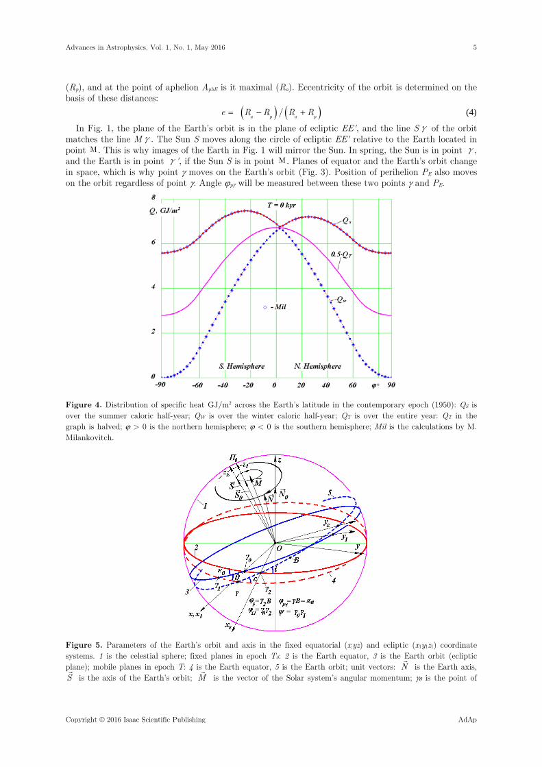
Figure 4. Distribution of specific heat GJ/m2 across the Earth’s latitude in the contemporary epoch (1950): QS is over the summer caloric half-year; QW is over the winter caloric half-year; QT is over the entire year: QT in the graph is halved; > 0 is the northern hemisphere; < 0 is the southern hemisphere; Mil is the calculations by M. Milankovitch.

Figure 5. Parameters of the Earth’s orbit and axis in the fixed equatorial (x,yz) and ecliptic (x1y1z1) coordinate systems. 1 is the celestial sphere; fixed planes in epoch T0: 2 is the Earth equator, 3 is the Earth orbit (ecliptic plane); mobile planes in epoch T: 4 is the Earth equator, 5 is the Earth orbit; unit vectors: N

is the Earth axis,

S

is the axis of the Earth’s orbit; M

is the vector of the Solar system’s angular momentum; is the point of



vernal equinox in ear T0; B is the position of perihelion on the celestial sphere; = 02 is the angular distance of the orbit’s ascending node; р = 2B is the angular distance of perihelion; i is the angle of inclination of the orbital plane against the plane of fixed equator.

New understanding of the orbital motion [21] has led to the development of an algorithm for calculating parameters r and λ that determine the value of daily insolation (2). A program was developed to calculate insolation on any day of the year, during a season, half-year, and year [19][20]. This program also enables determination of other elements of insolation. Fig. 4 describes the change by latitude φ° of the summer QS, winter QW and halved annual QT insolation in the contemporary epoch. Annual insolation QT declines steadily from the equator towards the poles. At the poles, the value of insolation is 2.4 times smaller than at the equator. Winter insolation QW near the equator is maximal, shrinking to zero at the poles. Summer insulation QS is maximal near the tropical latitudes ( = = 23.4) and minimal at the poles. In the contemporary epoch, summer insolation QS at the North Pole is smaller than at the South Pole, as shown in Fig. 4. Also, summer insolation in the northern tropics is 1.04 times smaller than in the southern tropics.

The program used for calculation of all the insolation elements can be freely accessed at http://www.ikz.ru/~smulski/Data/Insol/ [20]. It is based on our insolation calculation algorithm which is more convenient than the one developed by Milankovitch. In terms of quantity, the results of these two theories typically coincide, as shown in Fig. 4.

Angular parameters and distance that are part of the daily insolation formula (2) depend on the parameters of the Earth’s orbit and axis of its rotation, which tend to change in time, as stated above. Circles on the celestial sphere in Fig. 5 demonstrate planes of the Earth’s equator 2 and orbit 3 fixed in a certain epoch, such as year 2000. The angle between these planes equals 0. In a different epoch, the equator plane will move to position 4, and the orbit plant – to position 5, and the angle between these planes will equal . Seeking to determine behavior of parameters included in the formula of insolation (2), we must solve two tasks, specifically calculate the change of 1) orbital and 2) rotational motion.

4 Evolution of Orbital Motion

Subject to the law of universal gravitation, body k attracts body i with the following force:

3

i kik ik

ik

m mF G r

r

(5)

where G is the gravitational constant; ikr is radius vector from the body with mass mk to the body with mass mi.

All other k-bodies exert force (5) on the i-body. When we add up all the action forces and divide the resulting value by the mass of the i-body, we obtain such body’s acceleration as follows:

2

2 3

d, 1 ,2, , ,

d

ni k ik

k i ik

ir m r

Gt r

n

(6)

where ir is the radius vector of body im relative to a center in a nonaccelerating coordinate system

(in our case, relative to the Solar system’s center of mass). Equation (6) is a system of 3n nonlinear differential equations, where n = 11 (nine planets, the Sun

and the Moon). A high-precision method was developed to solve these equations, and it was later used to develop the Galactica system [22], which is free for access [23]. Viability of this method is confirmed by the solution of a number of problems in the contemporary celestial and space dynamics [24] - [28].

Evolution of the orbit is considered in a fixed coordinate system xyz associated with the fixed plane of equator 2 (see Fig. 5). In this study, we examine the evolution of orbit eccentricity e, angle of its inclination i against the plane of equator 2, and φ = γ0γ2, ascending node of orbit 2, and angular position of perihelion р = 2B, where B is the projection of perihelion on the celestial sphere 1.

The points in Fig. 6 represent the dynamics of elements the Earth’s orbit, i.e. eccentricity e and angles , i and р. Within the period of 7 thousand years (from –3.4 thousand years to 3.6 thousand years), eccentricity e and orbit inclination i decrease, while the angle of perihelion р increases. At the same time, the angle of ascending node decreases in the beginning of the period, and then begins to



increase. The minimum of occurs one thousand years before December 30, 1949. Unlike other parameters, the angle of perihelion р changes irregularly. Lines 2 and 3 in Fig. 6 describe the average changes of these parameters, which are derived by S. Newcomb [29], J. L. Simon et al. [30] from observations. The graphs demonstrate that calculation results are confirmed by observations.

Figure 6. Secular changes of the Earth’s orbit 1 and comparison with the approximations 2 and 3 of observation data obtained by S. Newcomb [29] and J.L. Simon et al. [30], respectively: e is the eccentricity; i is the inclination of orbit plane to equator plane of 2000.0; is the angular position of ascending node of orbit from axis x in the epoch of 2000.0; p is the angular position of perihelion in the plane of orbit from ascending node; all angles are in radians, and time T is in centuries from December 30, 1949; the gap between points is 200 years; 1 cyr equals one century.

Figure 7. Evolution of the Earth’s orbit in the past 3 million years. Designations are the same as in Fig. 6. Values with subscript m represent mean values of parameters over 50 million years; Тe, Тi, ТΩ represent the main periods of oscillations of corresponding parameters in thousands and millions of years, and Тp is the mean period of perihelion evolution in 3 million years; the gap between points is 10 thousand years; kyr is one thousand years; Myr is one



million years.

The evolution of the Earth’s orbit parameters over the past three million years is shown in Fig. 7. The eccentricity undergoes short-term changes with mean period Te1 = 94.5 thousand years around its mean value em = 0.028. Some longer oscillations also occur with the period Te2 = 413 kyr, which result in extreme values of eccentricity e = 0.0022 and e = 0.062. Longitude of ascending node φΩ changes with a mean period TΩ = 68.7 thousand years around its mean value φΩ т = 0.068 radian. Oscillations with longer duration superimpose on the main period.

The inclination angle of orbit plane undergoes changes with the same period T= 68.7 thousand years around its mean value m = 0.402 radian. Oscillations of angle i occur within the limits of 0.36 to 0.45 radian and the range of oscillations is 5º.

Perihelion position angle φр increases in time. Perihelion moves in the direction of the Earth’s evolution about the Sun, with one full evolution in 147 thousand years on average in 3 million years. Perihelion evolution is irregular. In addition to mean counterclockwise evolution, perihelion also shows reverse clockwise motion.

Analysis of the resulting solutions demonstrated that the axis of the Earth’s orbit S (see Fig. 5)

rotates clockwise, i.e. in counter-direction of the orbital motion of the Earth, with the period TS = -68.7 thousand years. Let's remind that the axis of the orbit S

is perpendicular to its plane 5. This rotation

results in the oscillations of angles i and φΩ shown in Fig. 7. The axis of the orbit S rotates around

the vector M

(Fig. 5), which is the angular momentum of the entire Solar system.

Figure 8. The evolution of the Earth’s orbit parameters in the past 50 million years: es is the sliding average of eccentricity; φp is the angle of perihelion; s is the angle of precession; and Ss are sliding average values of the inclination angle of orbital axis S

. Angles р and s are in radians, and Ss is in degrees.

Differential equations of orbital motion (6) were integrated using the Galactica software for the period of 100 million years. It is impossible to represent the resulting calculations with the previous parameters at this period, because their oscillations merge into a continuous band. This is why Fig. 8 shows evolution of the Earth’s orbit parameters over the period of 50 million years in a somewhat different format. Sliding average values of eccentricity es averaged over an interval of 2Te2 850 ≈ kyr. As we see from the graph, there is a third period of change of eccentricity Te3 = 2.31 Myr. Instead of angles of orbit i and φΩ, Fig. 8 shows evolution of angles Ss and S of the orbital axis S

relative to

vector M

(see Fig. 5). The angle of inclination Ss, which is also represented as a sliding average value, is the angle between vectors S

and M

.



Maximum deflection of axis S from moment M

is Smax = 2.94º. The periods of its oscillation are

as follows: T1 = 97.4 kyr, T2 =1.16 Myr and T=2.32 Myr. Oscillations with these periods are shown in Fig. 8. The angle of precession S is identical to angle φΩ, but it changes in the plane perpendicular to angular momentum M

instead of the plane of equator 2. Similar to the angle of perihelion φр, the

angle of precession S changes irregularly, with reverse movements. However, these oscillations of φр and S cannot be seen in the scale shown in Fig. 8. Due to irregular rotation, average periods of perihelion and orbital axis S

within the period of -50 million years are slightly different: Tp = 150

thousand years, and TS = -72.9 thousand years, respectively. The variation of parameters within the period from -50 million years to -100 million years is identical

to that shown in Fig. 8 [31]. Similar studies were carried out for all other planets and the Moon [28][32][33]. The parameters of their orbits change steadily, like the parameters of the Earth’s orbit. This leads to the conclusion that there are no other periods and amplitudes of oscillation of orbit parameters except those identified. The obtained results also indicate that the Solar system is stable. It should also be noted that the studies of other researchers [34] - [36], who used other methods to solve this problem, demonstrated changing oscillations. This is why they concluded that orbits and the Solar system in general are unstable [36].

Note that our integration results and orbit parameters of all planets for 100 Myr are available at http://www.ikz.ru/~smulski/Data/OrbtData/.

5 Evolution of Rotational Motion of the Earth

Under the influence of centrifugal forces, rotating Earth elongates in the plane of equator (see Fig. 9). Let us look at the impact of body B on two halves of the Earth, i.e. the action of force 1F

on the near

half and force 2F

on the far half. If the Earth was a centrally symmetrical sphere, the resultant of forces 1F

and 2F

would pass the Earth through its center O. For the oblate Earth, the center of

masses of the near part of the Earth will tend towards the body B, and the far part will tend away from it. This is why force 1F

will grow, and force 2F

will shrink, resulting in the clockwise moment of forces

mO. This process of action on the Earth is described by the theorem of change of angular momentum:

d

( )d

OO k

Km F

t

(7)

where OK

is the angular momentum of the Earth relative to the center O in a nonrotating coordinate system x1y1z1, and ( )O km F

is the total of the moments of forces exerted by bodies acting on the Earth.

Figure 9. The precession of the Earth’s axis under the influence of body B: 1 and 2 are planes of the Earth’s equator and orbit, respectively; 3 is the plane of the orbit of body B acting on the Earth.

The problem of the Earth’s rotation must be solved (see Fig. 5) in a nonrotating coordinate system x1y1z1 associated with the fixed plane of the Earth’s orbit 3. Moving plane of the Earth’s equator 4 is determined by the angle of inclination to the plane 3 and angle of precession =γ0γ1. The velocity of the Earth’s rotation relative to its moving axis N

must be considered as well. Based on the

theorem (7), we obtained [37][38] differential equations of the Earth’s rotational motion:



2 2

1 151

1 1 1 1 1

3cos2 0.5 sin(2 )( )sin sin

cos cos(2 ) ( cos sin )sin

nz E i d z

i iix i x

i i i i i

J GM E Jx y

J r J

x y z x y

(8)

2 2 2

151

2 2 21 1 1 1 1 1 1

sin 30.5 sin(2 ) sin(2 ) sin

2 cos sin(2 ) 2 ( sin cos )cos(2 ) ,

nz E i d z

iix i x

i i i i i i i

J GM E Jx

J r Jy z x y z x y

(9)

cosE (10)

where Jx, Jy and Jz are the moments of inertia of rotating Earth on the axes of the coordinate system associated with the rotating Earth; ( ) /d z x zE J J J is the dynamic ellipticity of the Earth; E =

const is the projection of absolute velocity of the Earth’s rotation onto its axis N

(see Fig. 5) n is the number of bodies acting on the Earth, Mi is the mass of such bodies, and x1i, y1i, z1i are their coordinates.

Equations (8) and (9) result in the angles of position and of the moving plane of equator 4 relative to the plane of fixed orbit 3 (see Fig. 5). Integration of equations (8)-(9) results in the angles of inclination and precession of moving equator 4 relative to the fixed plane of orbit 3. Integration of the equations of orbital motion (6) results in the angles of inclination i and ascending node φΩ of moving plane of orbit 5 relative to the fixed plane of equator 2, as well as the angle of perihelion φр. These parameters of angular and orbital motion help determine the angles of obliquity and perihelion φpγ of the moving plane of orbit 5 relative to the moving equator 4. Evolution of these angles , φpγ and eccentricity e defines the evolution of insolation.

Let us look at the basic results of solving the Earth rotation problem (8)-(9). Fig. 10 shows the change of obliquity in five different intervals In. The graphs demonstrate main periods Tni and amplitude (ai and a4 of oscillation of the inclination angle: half-month Tn2, six-month Tn3 and Tn4 = 18.6 years. These oscillations are known as nutation oscillations. The angle of precession has similar periods of oscillation, and its amplitudes are 2-3 times greater.

Figure 10. Changes of inclination angles and (in radians) of the Earth’s equator plane to its orbit in five time intervals In: yr is year; - 0; 0 is the obliquity in the initial epoch of December 30, 1949; Tn2, Tn3, Tn4 and a2, a3, a4 are periods and amplitudes of oscillation of the obliquity ; 1 is based on our results of numerical



integration; 2 is the approximation of observation data obtained by S. Newcomb [29] and J. Simon et al. [30]; 3 is based on the results of integration by Laskar, Robutel et al. [12]; 4 is based on the results of integration by S.G. Sharaf and N.A. Budnikova [10].

In the interval In = 0.1 year, we see half-monthly oscillations and daily oscillations; six-month oscillations occur in the interval In = 1 year; the interval In = 10 years already shows the trend of oscillations with the period of 18.6 years, and oscillations with this period prevail in the interval In = 100 years.

In the interval In = 100 years, we see that the calculated 1 obliquity oscillates about the average 2 obliquity determined by S. Newcomb [29] and J. Simon et al. [30]. The amplitude of oscillations a4=9.2˝ for the period Tn4=18.6 years also agrees with the observation results. This amplitude is known in astronomy as the constant of nutation. The calculated angle of precession also fluctuates about the averaged angle of precession observed, and the average change of agrees with observation results.

As one can see in Fig. 10, the approximated observation results coincide with the results obtained by other authors [10][12] in the range of up to 2000 years within interval In = 10 thousand years. After this, the obliquity that we calculated begins to differ from the results of solutions [10][12].

Fig. 11 demonstrates that differences grow in time, and further evolution of the calculated obliquity varies significantly from the evolution results obtained by other authors who solved a simplified problem of the Earth’s rotation. The graphs show that oscillations of angle in our solutions occur within the range of 16.7º to 31º, while previous solutions result in the oscillation range of 22.26º to 24.32º, i.e. the range of oscillations is 7 times greater. We calculated the Earth’s insolation with new evolution of angle [17] Its oscillations are also 7 times greater than oscillations of insolation according to previous astronomical theories of paleoclimate.

The second angle in equations (8) - (10), i.e. the angle of precession , varies in a different manner than the angle . It decreases continuously, but this decrease occurs with the same oscillations as for angle , only the amplitude of oscillations is 2-3 times greater. This change of angle proves that the Earth’s axis N

(see Fig. 5) rotates clockwise, and the average period of its rotation is PN = -25740

years. Existing studies of these two problems formulate the following vision of motion in the Solar system.

Perihelion rotates irregularly counterclockwise in the plane of the orbit with a mean period Tp = 147 kyr, and deformation of the orbit occurs with oscillations of eccentricity with the periods of 94.5 kyr, 413 kyr and 2.31 Myr. Similar changes of orbit with their own periods occur to the Moon and other planets, except Pluto. Perihelion of Pluto rotates in a clockwise direction.

Figure 11. The evolution of obliquity (in radians) of the plane of the Earth’s equator to the plane of its orbit in the interval of 200 thousand years: 1 is based on our results of numerical integration; 2 is based on the results of integration by Laskar, Robutel et al. [12]; 3 is based on the results of integration by S.G. Sharaf and N.A. Budnikova [10]. Maximum and minimum values of angle are indicated in degrees.

The axis of the Earth’s orbit S (see Fig. 5) rotates clockwise about the vector of moment M

with

average period TS = 68.7 kyr over 3 million years. Axis S also fluctuates with different periods of 97.4

kyr, 1.16 Myr and 2.32 Myr. The axis of the Moon’s orbit (not shown in Fig. 5) rotates clockwise about the moving axis S

of the Earth’s orbit. The period of this rotation is 18.6 years. Also, the axis of the

Moons’ orbit fluctuates with the period of 0.4745 years.



As stated above, the Earth’s axis of rotation N

(see Fig. 5) rotates clockwise with a mean period of 25740 years. Axis N

fluctuates with a half-month, six-month and 18.6 year periods. Besides, wide-

amplitude oscillations of axis N

occur (see Fig. 11) with periods of tens and hundreds of thousand years. During these oscillations, the obliquity of the Earth’s axis varies from 16.7° to 31°, while according to the previous theories it varies from 22.26 to 24.32. In other words, the range of the Earth’s axis oscillations increased seven-fold.

6 Evolution of Insolation

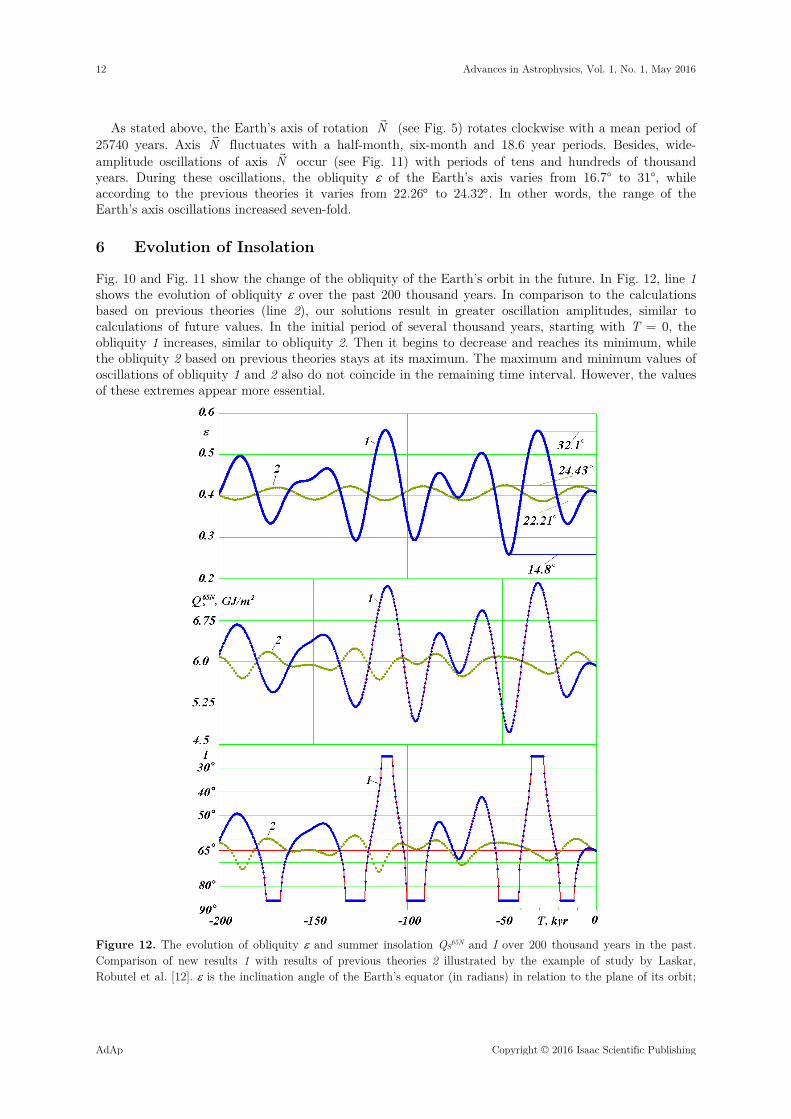
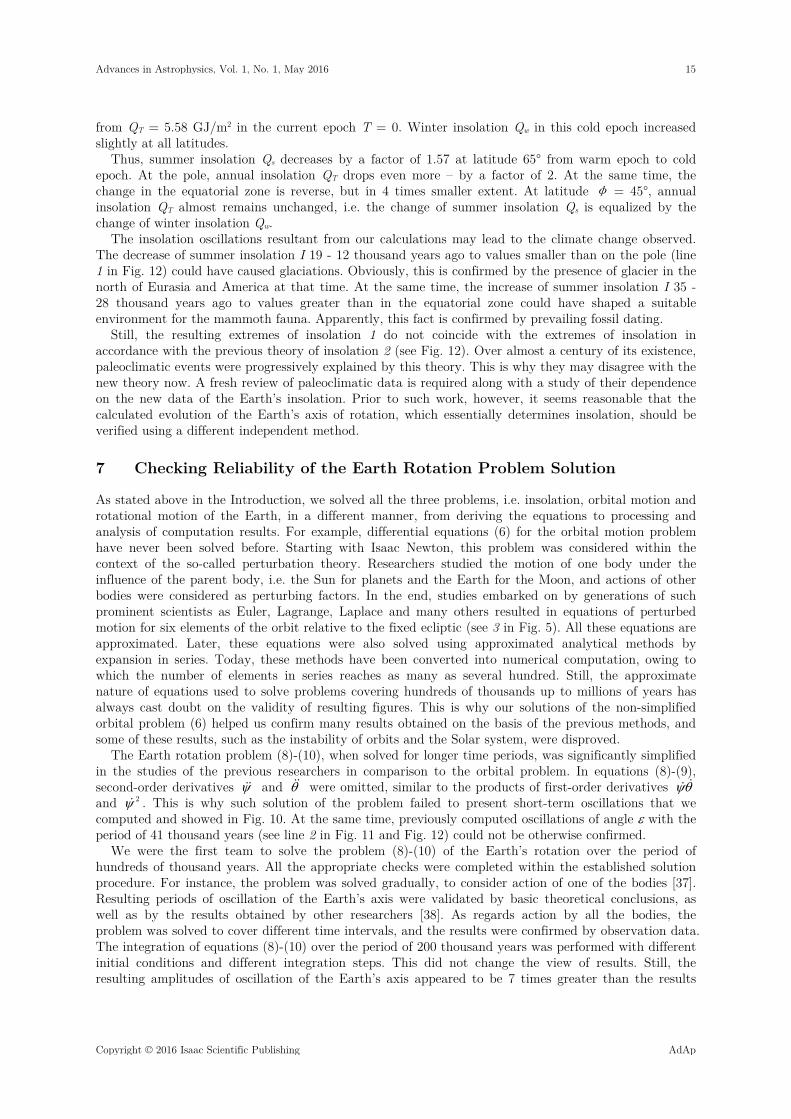
Fig. 10 and Fig. 11 show the change of the obliquity of the Earth’s orbit in the future. In Fig. 12, line 1 shows the evolution of obliquity over the past 200 thousand years. In comparison to the calculations based on previous theories (line 2), our solutions result in greater oscillation amplitudes, similar to calculations of future values. In the initial period of several thousand years, starting with T = 0, the obliquity 1 increases, similar to obliquity 2. Then it begins to decrease and reaches its minimum, while the obliquity 2 based on previous theories stays at its maximum. The maximum and minimum values of oscillations of obliquity 1 and 2 also do not coincide in the remaining time interval. However, the values of these extremes appear more essential.

Figure 12. The evolution of obliquity and summer insolation QS65N and I over 200 thousand years in the past. Comparison of new results 1 with results of previous theories 2 illustrated by the example of study by Laskar, Robutel et al. [12]. is the inclination angle of the Earth’s equator (in radians) in relation to the plane of its orbit;



QS65N is the insolation (GJ/m2) over the summer caloric half-year period on the northern latitude of 65; I is the insolation in equivalent latitudes over the summer caloric half-year in the northern latitude of 65. Maximum and minimum values of angle are indicated in degrees.

In accordance with previous theories, the obliquity changes from 22.21 to 24.43 during this time interval. Based on our solutions, the inclination of the Earth’s equator plane in relation to the plane of its orbit varies from 14.8 to 32.1. In this case, the range of oscillations of new solutions becomes 7.8 times higher. Astronomical theories of paleoclimate study insolation over equal caloric half-year periods instead of astronomic half-year periods. The beginning and the end of the summer caloric half-year period is determined so as to make sure that insolation on any of its day is greater than insolation on any day of the winter half-year. Below we will study insolation on the latitude of 65° of the northern hemisphere, which is marked as N. We calculate the change of insolation QS

65N over 200 thousand years in the past both on the basis of our identified parameters e, and φpγ (line 1 in Fig. 12), and on the basis of the same parameters calculated by Laskar, Robutel et al. [12] (line 2). As one can see in the graphs, insolation QS

65N over the summer caloric half-year period in northern latitude of 65 based on our solutions occurs with the oscillation amplitude that is 7 times greater than that calculated on the basis of previous theories. The time of warm spells and cold spells based on our calculations (1) and previous theories (2) do not coincide, as well. In the beginning, starting with T = 0, as we see from QS

65N in Fig. 12, summer insolation grows during 4-5 thousand years, and then it begins to decrease, reaching its minimum 16 thousand years ago. This minimum is followed by a warm spell, which ends in the greatest maximum of insolation 31 thousand years ago.

The average period of the obliquity oscillations in accordance with previous theories (see 2 in Fig. 12) is 41.1 thousand years. The same period is true for the oscillation of insolation QS

65N (line 2). As we see from the new equation, the obliquity (line 1) typically has a 1.5-2 times shorter period of oscillations.

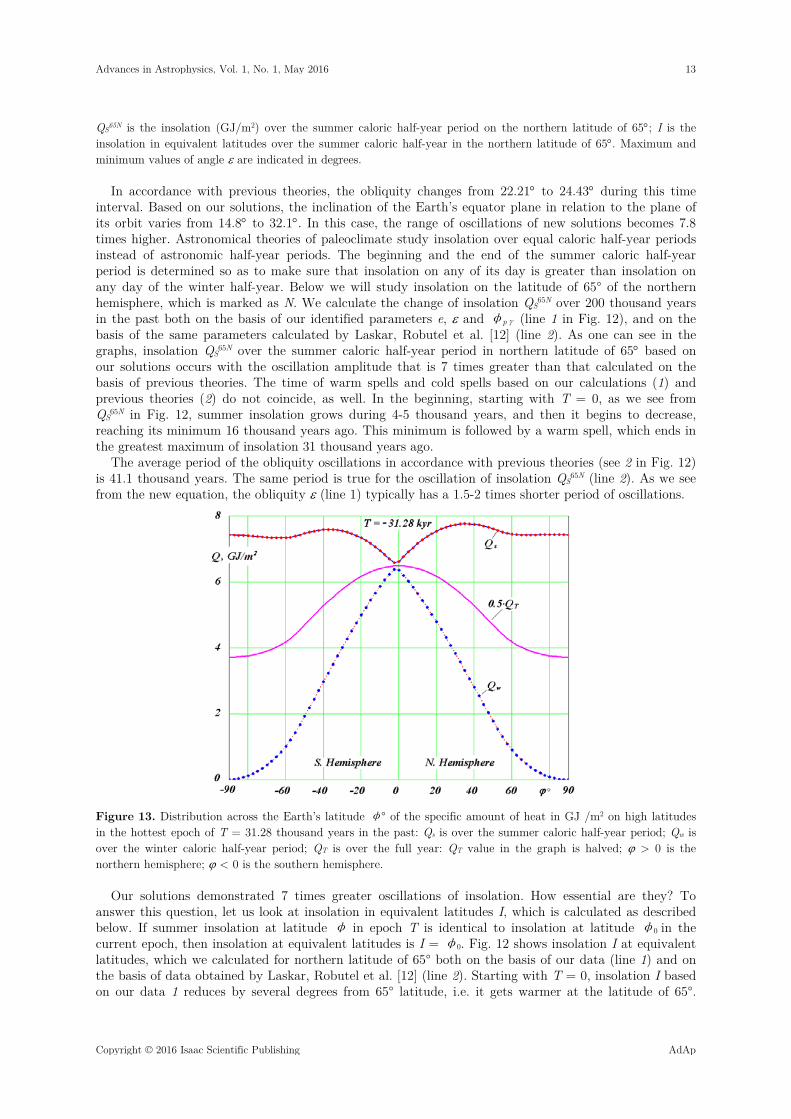
Figure 13. Distribution across the Earth’s latitude φ° of the specific amount of heat in GJ /m2 on high latitudes in the hottest epoch of T = 31.28 thousand years in the past: Qs is over the summer caloric half-year period; Qw is over the winter caloric half-year period; QT is over the full year: QT value in the graph is halved; > 0 is the northern hemisphere; < 0 is the southern hemisphere.

Our solutions demonstrated 7 times greater oscillations of insolation. How essential are they? To answer this question, let us look at insolation in equivalent latitudes I, which is calculated as described below. If summer insolation at latitude φ in epoch T is identical to insolation at latitude φ0 in the current epoch, then insolation at equivalent latitudes is I = φ0. Fig. 12 shows insolation I at equivalent latitudes, which we calculated for northern latitude of 65° both on the basis of our data (line 1) and on the basis of data obtained by Laskar, Robutel et al. [12] (line 2). Starting with T = 0, insolation I based on our data 1 reduces by several degrees from 65° latitude, i.e. it gets warmer at the latitude of 65°.



After I reaches its maximum, it starts decreasing towards latitudes of 80° and 90°. For T = -15 thousand years, the summer insolation at the latitude of 65° is smaller than the current summer insolation at the pole, which is why graph I shows a horizontal line. Thus, the horizontal line approximately 15 thousand years ago shows that the insolation at the latitude of 65° is smaller than at the pole today. This small amount of heat could lead to glaciations of territories at the latitude of 65°.

Later, towards T = -30 kyr, insolation I at the equivalent latitudes reaches the latitudes of 50°, 40° and 30°, i.e. the latitude of 65° gets much more sunlight. Horizontal line in the epoch of T = -30 kyr means that 65° latitude gets more heat than the equator today.

Line 2 shows insolation I at the equivalent latitudes in accordance with the previous theories. As we see, the summer insolation at the latitude of 65 over the time period of 30 - 50 thousand years varies within the limits of 60 to 70. It is unlikely that the change in the amount of heat at the 65 latitude to the values true for the latitudes of 60 and 70 today may lead to any substantial warming or cooling of the climate. These insignificant changes of insolation have always been doubtful [7].

In the text above, we studied the change of insolation in time at the northern latitude of 65°. Let us now look at the change of insolation by latitude at certain points in time. Fig. 4 shows distribution of insolation across the globe in the current epoch. Fig. 13 shows the change of summer Qs, winter Qw and halved annual QT insolation by latitude φ° in the epoch T = -31.28 thousand years. This time is marked by the most intensive summer insolation over 200 thousand years at 65°N (see Fig. 12). Just like in the current epoch (see Fig. 4), annual insolation QT is the greatest at the equator, gradually decreasing towards the poles. Winter insolation Qw is maximal near the equator, tending to zero at the poles. The summer insolation is maximal in the tropics, which were then at higher latitudes than in the current epoch (see Fig. 4). Furthermore, the summer insolation at high latitudes is close to maximal and is significantly greater than the summer insolation at the equator.

Annual insolation QT in epoch T = -31.28 thousand years at high latitudes is greater (Fig. 13) than in the current epoch (Fig. 4). At the same time, the annual insolation at the equator is less than in the current epoch. Still, this reduction is not as significant as at high latitudes. Winter insolation Qw in epoch T = -31.28 thousand years at all latitudes is less than in the current epoch (Fig. 4).

Figure 14. Distribution across the Earth’s latitudes φ° of specific amount of heat in GJ/m2 in the coldest epoch of T = 46.44 thousand years in the past for high latitudes. Other designations see Fig. 13.

Fig. 14 shows the change of the same elements of insolation in the coldest epoch of T = -46.44 thousand years over the 200-thousand-year period. At high latitudes, such as φ° = 65°N, summer insolation Qs = 4.72 GJ/m2 has decreased substantially versus Qs = 7.43 GJ/m2 in the epoch T = -31.28 thousand years and Qs = 5.92 GJ/m2 in the current epoch T = 0. Annual insolation, such as QT = 3.58 GJ/m2 at the North Pole, dropped from QT = 7.43 GJ/m2 in the epoch T = -31.28 thousand years and



from QT = 5.58 GJ/m2 in the current epoch T = 0. Winter insolation Qw in this cold epoch increased slightly at all latitudes.

Thus, summer insolation Qs decreases by a factor of 1.57 at latitude 65° from warm epoch to cold epoch. At the pole, annual insolation QT drops even more – by a factor of 2. At the same time, the change in the equatorial zone is reverse, but in 4 times smaller extent. At latitude φ = 45°, annual insolation QT almost remains unchanged, i.e. the change of summer insolation Qs is equalized by the change of winter insolation Qw.

The insolation oscillations resultant from our calculations may lead to the climate change observed. The decrease of summer insolation I 19 - 12 thousand years ago to values smaller than on the pole (line 1 in Fig. 12) could have caused glaciations. Obviously, this is confirmed by the presence of glacier in the north of Eurasia and America at that time. At the same time, the increase of summer insolation I 35 - 28 thousand years ago to values greater than in the equatorial zone could have shaped a suitable environment for the mammoth fauna. Apparently, this fact is confirmed by prevailing fossil dating.

Still, the resulting extremes of insolation 1 do not coincide with the extremes of insolation in accordance with the previous theory of insolation 2 (see Fig. 12). Over almost a century of its existence, paleoclimatic events were progressively explained by this theory. This is why they may disagree with the new theory now. A fresh review of paleoclimatic data is required along with a study of their dependence on the new data of the Earth’s insolation. Prior to such work, however, it seems reasonable that the calculated evolution of the Earth’s axis of rotation, which essentially determines insolation, should be verified using a different independent method.

7 Checking Reliability of the Earth Rotation Problem Solution

As stated above in the Introduction, we solved all the three problems, i.e. insolation, orbital motion and rotational motion of the Earth, in a different manner, from deriving the equations to processing and analysis of computation results. For example, differential equations (6) for the orbital motion problem have never been solved before. Starting with Isaac Newton, this problem was considered within the context of the so-called perturbation theory. Researchers studied the motion of one body under the influence of the parent body, i.e. the Sun for planets and the Earth for the Moon, and actions of other bodies were considered as perturbing factors. In the end, studies embarked on by generations of such prominent scientists as Euler, Lagrange, Laplace and many others resulted in equations of perturbed motion for six elements of the orbit relative to the fixed ecliptic (see 3 in Fig. 5). All these equations are approximated. Later, these equations were also solved using approximated analytical methods by expansion in series. Today, these methods have been converted into numerical computation, owing to which the number of elements in series reaches as many as several hundred. Still, the approximate nature of equations used to solve problems covering hundreds of thousands up to millions of years has always cast doubt on the validity of resulting figures. This is why our solutions of the non-simplified orbital problem (6) helped us confirm many results obtained on the basis of the previous methods, and some of these results, such as the instability of orbits and the Solar system, were disproved.

The Earth rotation problem (8)-(10), when solved for longer time periods, was significantly simplified in the studies of the previous researchers in comparison to the orbital problem. In equations (8)-(9), second-order derivatives and were omitted, similar to the products of first-order derivatives and 2 . This is why such solution of the problem failed to present short-term oscillations that we computed and showed in Fig. 10. At the same time, previously computed oscillations of angle with the period of 41 thousand years (see line 2 in Fig. 11 and Fig. 12) could not be otherwise confirmed.

We were the first team to solve the problem (8)-(10) of the Earth’s rotation over the period of hundreds of thousand years. All the appropriate checks were completed within the established solution procedure. For instance, the problem was solved gradually, to consider action of one of the bodies [37]. Resulting periods of oscillation of the Earth’s axis were validated by basic theoretical conclusions, as well as by the results obtained by other researchers [38]. As regards action by all the bodies, the problem was solved to cover different time intervals, and the results were confirmed by observation data. The integration of equations (8)-(10) over the period of 200 thousand years was performed with different initial conditions and different integration steps. This did not change the view of results. Still, the resulting amplitudes of oscillation of the Earth’s axis appeared to be 7 times greater than the results



based on the previous theories, which required the results to be confirmed. Apparently, a different way should be used to solve this problem. For several years, we have been trying to define and implement such ways of solving the problem.

The problem of the Earth rotation is one of the most complicated problems in mechanics. This is confirmed by the way equations (8)-(10) look. Their derivation involves a number of conversions from one coordinate system into another, as well as a number of simplifications and approximations. This is why the results could be verified cardinally if they were obtained without solving the differential equations (8)-(9).

When studying the orbits, we discovered that the evolution of the Moons’ orbit axis is similar to evolution of the Earth’s axis of rotation. This result led us to the compound model of the Earth (see Fig. 15), where a portion of the Earth’s mass is equally distributed among circumferential bodies orbiting around the central body on a circular orbit. Orbits of circumferential bodies begin to change under the action of the Moon, the Sun and planets. Evolution of orbital axis of one of these bodies reflects evolution of the Earth’s axis of rotation. In the first series of studies [25], three models were investigated, confirming the possibility to simulate evolution of the Earth’s axis. In these models, the periods of precession of model orbit axes equaled 170 years and 2,604 years, while average period of precession of the Earth’s axis TprE = 25,740 years. Eleven other models were developed later, until the desired period of precession was obtained.

Figure 15. Compound model of the Earth’s rotation. The Earth’s mass is distributed among the central body and circumferential bodies: a – circumferential bodies’ orbital radius.

This simulation of the Earth’s rotation involves several stages of solving the orbital problem (6) using the Galactica software. It appears that the model with desired period of precession can be obtained if gravitational interaction among the model bodies is reduced or increased. Thus, the Galactica software was developed with the modified interaction among certain bodies.

Figure 16. The evolution of angles of obliquity and precession of rotation axis of the Earth’s compound model No. 13 over 300 years. The points in the figure represent the results of integration of equations (6) using Galactica. The distance between the points is 3 years. The lines represent mean changes of angles and ψ at the rate 300m =

- 2.28·10-4 1/cyr = - 0.470 ˝/yr; 300m = - 2.42·10-2 1/cyr = - 49.9 ˝/yr.



The points in Fig. 16 show results of the 13th compound model of the Earth for the period of 300 years. As one can see, the obliquity and precession angle vary with the period of 18.6 years. Solutions for shorter time periods resulted in oscillations with half-month and half-year periods, i.e. these results coincided with the results of the integration of equations (8)-(10). The amplitudes of these oscillations also coincide. Straight lines in Fig. 16 identify mean changes of angles and . They also coincided with the results of direct problem of the Earth rotation, as well as with the observation data. Equivalence of results is also obvious if one compare Fig. 16 with the graph of angle for the interval of 100 years in Fig. 10.

This similarity between the results of the model problem and the results of direct problem occurs in the period of up to 3 thousand years. Then equations (6) are integrated in the Galactica software, errors accumulate for model bodies, and the model dimensions start changing. The orbit’s period of precession also changes. For example, by the end of the integration interval of 13.763 thousand years, the period of precession reduced from 25740 years to 14840 years, and the model no longer represents the evolution of the Earth’s axis. This process occurs due to highly intense dynamic parameters of the model. For instance, the orbital radius of circumferential bodies a (see Fig. 15) equals the Earth’s radius, their orbital period is 0.142 hours, and the interaction between the model bodies is 9.6 times stronger than the gravitational interaction. Thus, the model bodies rotate 170 times faster than the Earth. This is why the integration step of problem (6) must be reduced 1000-fold compared to the step used in solving the orbital problem. This results in a long time of computation. For example, it took 2.13 months to compute the problem over the period of 13.763 thousand years. To make sure the model does not change in the interval of 200 thousand years, integration step must be reduced to such values that will require unpractical computation time.

At this stage, compound model covering 3000 years confirmed the results for integration of differential equations (8)-(10) of the Earth’s rotation. This proves the assumptions and simplifications made during the derivation of equations (8)-(10), their derivation, solution method and conversion of integration results into the final view.

The second independent verification involved the use of a more precise method during the integration of equations (8)-(10), specifically the 8th order Runge-Kutta method in the interpretation of Dormand and Prince [39]. Previously, the DfEqAl1-.for program used a 4th order Runge-Kutta integration method [40]. We were using it for several decades to solve various problems, and the results were always satisfactory. When integrating equations of rotational motion (8)-(10) over time intervals of some 200 thousand years, we faced an unexpected shortfall of this method. Solutions of these equations show daily oscillations of derivatives of and . Amplitude of these oscillations by the end of the specified interval of integration increased by several orders. Despite the tests to check the impact of daily amplitudes of and on the end results and certain steps to eliminate such impact, the threat of their accidental impact still remained.

A program DfEqADP8-.for was developed, to solve the Earth rotation problem based on the Dormand and Prince method and equations (8)-(10) were integrated at different intervals, including 200 thousand years. All the previous results were confirmed. The amplitudes of daily oscillations of derivatives of and do not increase and remain on the same level. Thus, equation integration method has no effect on the obtained results, and the results are confirmed through application of a more precise method.

The third independent verification implied the use of a different problem solution process. The differential equations of rotational motion (8)-(9) include coordinates x1i, y1i, z1i of bodies acting on the Earth that are associated with the plane of orbit. When solving the orbital problem (6) using Galactica, we calculate coordinates of bodies xi, yi, zi associated with the plane of fixed equator. They were converted into coordinates x1i, y1i, z1i. However, when we integrate the problem (8)-(9) over long time periods, the resulting data array will require impractical huge amount of memory. This is why we developed a mathematical model of the Solar system [21] that delivers, at the right time, coordinates of bodies x1i, y1i, z1i on the basis of results of two-body problem, i.e. the parent body and its satellite. In this case, parameters of the body’s orbit, including e, i, φΩ, φр, Rp, etc. at each point of time are determined on the basis of the data that were calculated prior in Galactica. When solving this task, we ran a comprehensive check of the Solar system’s mathematical model. Still, the possibility remained that, in case of long time intervals, insignificant differences of the results of the Solar system’s mathematical



model from the values of coordinates computed by Galactica may impact the evolution of rotational motion parameters and .

Working on the problem of the Earth’s rotation, we repeatedly tried using a different computation process. All our attempts were futile until we delivered an idea of effective consolidation of these two problems into one. As a result, we developed a new program, glc3rtc2.for, for the integrated solution of the orbital problem and the Earth rotation problem. In this program, a single step is used for solving the orbital problem (6) using Galactica and then to compute the Earth rotation problem (8)-(10) using the Dormand-Prince method. The new program helped us solve these two problems over different time periods, including the 200 thousand year interval. All the previous results were confirmed. This verification also proved the Solar system’s mathematical model over a long interval.

Table 1. Comparison of three methods of integrating the equations of rotational motion (8)-(9) over the past 200 thousand years: RG-4 is the 4th order Runge-Kutta method; DP-8 is the 8th order Runge-Kutta method in interpretation of Dormand-Prince; Gal is the coordinates of bodies included in equations (8)-(9), they are computed in Galactica, and the equations are solved using DP-8 method.

Method Ppr, yrs min max RG-4 -25774 14.806° 32.073° DP-8 -25774 14.806° 32.073° Gal -25749 14.802° 32.077°

Graphs in Fig. 12 obtained using the initial method were identical to graphs received by solving the

problem using the last two methods. Table 1 contains a quantitative comparison of the period of precession Ppr and the minimum min and maximum max angles of inclination, accurate to the fifth significant figure. The results of the third method, as seen from Table 1, vary in the 4th figure for the period of precession Ppr and in the 5th figure for the obliquity . While this is a higher-precision method, the last values represent the update to the results obtained using the first two methods.

Thus, miscellaneous tests and verifications of the initial method of solving the Earth rotation problem, as well as independent solutions of this problem using three other methods, confirmed that the Earth’s axis of rotation fluctuates with an amplitude 7 times greater than that previously computed by our predecessors.

Let us look at the new solutions of the Earth insolation problem once again. As shown in Fig. 12, both summer insolation QS

65N and insolation at equivalent latitudes I based on our calculations (line 1) varies significantly from insolation based on the previous theories (line 2) already at the initial time gap of 0 to -50 thousand years. According to the new solutions, the ice age could have occurred in the interval of 19 to 12 thousand years ago. It was preceded by a very warm period some 35 – 28 thousand years ago. These climate changes are confirmed by the research of A. S. Arkhipov (1928-1998) in the Upper Pleistocene of the West Siberia [41]. According to Arkhipov, “the Sartan glacial complex consists of moraines of the Gydan Stage and two recessive stages, i.e. Nyapan and Norilsk Stages. The apex of glaciations occurred 20-18 thousand years ago, the Nyapan stage 15-13 thousand years ago, and the Norilsk Stage 11.5-10.4 thousand years ago.” In the same study [41], the warm period mentioned above is confirmed by the following statement: “Radiometric age of the Karginsky interglacial (megastage) horizon dates back to the period from 55 - 50 to 23 - 22 thousand years ago, and this horizon contains a combination of marine and alluvial deposits, as well as staged lokhpodgort glacial, glaciolacustrine and terrestrial deposits…” As we see, a cold period 19 - 12 thousand years ago (see insolation I in Fig. 12, line 1) and a warm period 35 - 28 thousand years ago are consistent within the accuracy of the paleoevents dating.

Professor A. S. Arkhipov was famous for good reasoning behind his conclusions pertaining to the paleoclimate. This is why the results of his studies provided above deserve close attention, even though they disagreed with the results of the previous astronomical theory of paleoclimate (see 2 in Fig. 12). Except Arkhipov [41], other paleoclimatologists: Grosswald [42], Svendsen et al [43] and others had the same understanding of paleoclimate. However, their point of view was sinking in a sea of different theories of the majority of paleo-climatologists. As stated above, for almost one hundred years, paleoclimate researchers had to refer to the results of the previous astronomical climate theory. They



will now need to put substantial effort in reconsidering the entire body of data on paleoclimate, which will result in a more accurate definition of the Earth’s history.

8 Conclusion

The astronomical theory of ice ages, as originally suggested by its authors L. Agassiz [3], J. Adhemar [4], J. Croll [5], R. Hargreaeves [44], M. Milankovitch [6] and other researchers, can explain the occurrence of ice ages in the past in rotation with very warm periods. The theory should be studied further and expanded. On one hand, the solution of the problem of the Earth’s rotation over long intervals in the past must continue. On the other hand, existing results of oscillations of the Earth’s insolation must be used to analyze the evidence of paleoclimatic changes to identify if they are associated with oscillations of the Earth’s insolation.

Further studies of the astronomical theory of climate change on Mars [13][35] also appear interesting. The space exploration of its surface [45] proves that the planet used to have river beds, water basins and other evidence of warmer climate than there is now. It is possible that one of the reasons for climate change lies also in the oscillation of Mars rotation axis and parameters of its orbit.

9 Acknowledgement

This study began in 1995, and at different stages of the work helped me: O.I. Krotov, K.E. Sechenov, L.I. Smulsky, Ya.J. Smulsky and others. Computations were performed on the supercomputers of M.V. Keldysh Institute of Applied Mathematics of the Russian Academy of Sciences (Moscow) and the Siberian Supercomputer Center, the Siberian Branch of the Russian Academy of Sciences (Novosibirsk). The work was performed with support of grants provided by the Governor of Tyumen Region in 2003 and 2004, as well as the Integration Programme of the RAS Presidium No. 13 and ONZ-11 in 2004 – 2011. Throughout the study, it was supported by V.P. Melnikov, the Director of the Institute of the Earth Cryosphere. I hereby acknowledge the above colleagues and teams for their assistance.

References

1. B. John, E. Derbyshire, G Young., R. Fairbridge and J. Andrews, Winters of the World, In Russian, Ed. B. John, Moscow: Mir, 1982, 336 p.

2. J. Imbrie and K. P. Imbrie, Ice ages, Solving the Mystery. Earth under Ice Ages, In Russian, Ed. G. . Avsyuk, А

Moscow: Progress, 1988, 264 p. 3. L. Agassiz, Etudes sur les glaciers. Neuchatel, 1840. 4. J. A. Adhemar, Revolutions de la mer: Deluges Periodiques, Carilian-Goeury et V. 1842. Dalmont. Paris. 5. J. Croll, “On the physical cause of the change of climate during geological epochs,” Philosophical Magazine, 1864,

28, 121-137. 6. M. Milankovitch, Mathematische Klimalhre und Astronomische Theorie der Klimaschwankungen (Mathematic

Climatology and the Astronomical Theory of Climate Change). Gebruder Borntraeger, Berlin, 1930; GONTI, Moscow, 1939, 207 p.

7. V. A. Bol’shakov and A. P. Kapitsa, “Lessons of the Development of the Orbital Theory of Paleoclimate,” J Her. Russ. Acad. Sci., 2011, 81 (4), 387. Available: http://dx.doi.org/10.1134/S1019331611030014

8. D. Brauwer and A. J. J Van Woerkom, “The secular variation of the orbital elements of the principal planets,” Astron. Pap, 1950, (13), P. 2.

9. A. Woerkom, “The astronomical theory of climatic change,” in book: The Climate Change, oscow: I. I. L. 1958М , 168-178 (In Russian).

10. Sh. G. Sharaf and N. A. Budnikova, “Secular Changes in the Elements of the Earth’s Orbit and the Astronomical Theory of Climate Fluctuations,” in Proceedings of the Institute of Theoretical Astronomy (Nauka, Leningrad), 1969, vol. 14 (In Russian).

11. A. Berger and M. F. Loutre, “Insolation values for the climate of the last 10 million years,” Quaternary Science Reviews, 1991, 10, 297-317.



12. J. Laskar, P. Robutel, F. Joutel, M. Gastineau, A. C. M. Correia and B. Levrard, “A Long-term numerical solution for the Earth,” Icarus, 2004, 170, (2), 343-364.

13. S. Edvardsson, K. G. Karlsson and M. Engholm, “Accurate Spin Axes and Solar System Dynamics: Climatic Variations for the Earth and Mars,” Astronomy & Astrophysics, 2002, 384 689-701. Available: http://dx.doi.org/10.1051/0004-6361:20020029.

14. J. Adem, “Numerical Experiments on Ice Ages climates,” Climatic change, 1981, 3, 155-171. 15. L. E. Lisiecki and M. E. Raymo, “A Pliocene-Pleistocene Stack of 57 globally distributed benthic δ18O

records,” Paleocenography, 2005, 20 1-17. 16. CLIMAP Project Members. “The Surface of the Ice-Age Earth”, Science, 1976, 191, 1131-1137. 17. I. I. Smul'skii, “Analyzing the Lessons of the Development of the Orbital Theory of the Paleoclimate,” J Herald

of the Russian Academy of Sciences, 2013, 83, (1), 46-54. Available: http://dx.doi.org/10.7868/S0869587313010118.

18. J. J. Smulsky, The Theory of Interaction, Novosibirsk: Novosibirsk University, Scientific Publishing Center of UGG SB of RAS, 1999, 294 p. Available: http://www.ikz.ru/~smulski/TVfulA5_2.pdf (In Russian). English translation: J. J. Smulsky, The Theory of Interaction, PH Cultural Information Bank. Ekaterinburg, 2004302 p. Available: http://www.ikz.ru/~smulski/TVEnA5_2.pdf

19. J. J. Smulsky and O. I. Krotov, “New Computing Algorithm of the Earth's Insolation,” The Institute of the Earth Cryosphere SB RAS, Tyumen, 2013, 38 p., Dept. at VINITI 08.04.2013 No. 103-B2013. Available: http://www.ikz.ru/~smulski/Papers/NwAlClI2c.pdf. (In Russian).

20. J. J. Smulsky and O. I. Krotov, “New Computing Algorithm of the Earth's Insolation,” Applied Physics Research, 2014, 6, (4), 56-82. Available: http://dx.doi.org/10.5539/apr.v6n4p56.

21. J. J. Smulsky, “The Mathematical Model of Solar System,” in Col. The Theoretical and Applied tasks of the Nonlinear Analysis, Russian Academy of Sciences: A.A. Dorodnicyn Computing Center. Moscow, 2007, 119-138. Available: http://www.ikz.ru/~smulski/Papers/MatMdSS5.pdf (In Russian).

22. J. J. Smulsky, “Galactica Software for Solving Gravitational Interaction Problems,” Applied Physics Research, 2012, 4, (2), 110-123. Available: http://dx.doi.org/10.5539/apr.v4n2p110.

23. J. J. Smulsky, “The System of Free Access Galactica to Compute Interactions of N-Bodies,” I. J. Modern Education and Computer Science, 2012, 11, 1-20. Available: http://dx.doi.org/10.5815/ijmecs.2012.11.01

24. J. J. Smulsky, “Optimization of Passive Orbit with the Use of Gravity Maneuver,” Cosmic Research, 2008, 46, (5), 456–464. Available: http://dx.doi.org/10.1134/S0010952508050122. http://www.ikz.ru/~smulski/Papers/COSR456.PDF.

25. V. P. Mel’nikov, I. I. Smul’skii and Ya. I. Smul’skii, “Compound Modeling of Earth Rotation and Possible Implications for Interaction of Continents,” Russian Geology and Geophysics, 2008, 49, 851–858. Available: http://dx.doi.org/10.1016/j.rgg.2008.04.003. http://www.ikz.ru/~smulski/Papers/RGG190.pdf.

26. J. J. Smulsky, “New Components of the Mercury’s Perihelion Precession,” Natural Science, 2011, 3, (4), 268-274. Available: http://dx.doi.org/10.4236/ns.2011.34034, http://www.scirp.org/journal/ns.

27. I. I. Smul'skii, “Multilayer Ring Structures,” Physics of Particles and Nuclei Letters, 2011, (8), 5, 436-440. Available: http://dx.doi.org/10.1134/S1547477111050189. http://www.ikz.ru/~smulski/Papers/PHPL436.pdf.

28. J. J. Smulsky and Ya. J. Smulsky, “Dynamic Problems of the Planets and Asteroids, and Their Discussion,” International Journal of Astronomy and Astrophysics, 2012, 2, 129-155. Available: http://dx.doi.org/10.4236/ijaa.2012.23018.

29. S. Newcomb, The elements of the four inner planets and the fundamental constants of astronomy, Washington: Government printing office, 1895, 202 p.

30. Simon J. L. , Bretagnon P., Chapront J. et al 1994. Numerical Expression for Precession Formulae and Mean Elements for the Moon and the Planets. Astron. and Astrophys, 282, 663-683.

31. V. P. Melnikov and J. J. Smulsky, Astronomical theory of ice ages: New approximations. Solutions and challenges, Novosibirsk: Academic Publishing House “GEO”, 2009, 182 p. Available: http://www.ikz.ru/~smulski/Papers/AsThAnE.pdf.

32. J. J. Smulsky, “Calculation of Interactions in the Solar System over 50 Million Years to Study Climate Evolution,” Bolshaya Medveditsa, Journal of Problems of Earth Protection, Novosibirsk: Lomonosov Interregional Public Fund, 2005, 1, 44-56. Available: http://www.ikz.ru/~smulski/Papers/RasVSS2c.pdf (In Russian).



33. E. A. Grebenikov and J. J. Smulsky, “Evolution of Mars’s orbit over 100 Myr,” Papers on Applied Mathematics, Russian Acad. Sci., Dorodnitsyn Computing Center, Moscow, 2007, 63 p. Available: http://www.ikz.ru/~smulski/Papers/EvMa100m4t2.pdf (In Russian).

34. A. Morbidelli, “Modern Interactions of Solar System Dynamics,” Annul Rev. Earth planet. Sci., 2002, 30, 89-112.

35. J. Laskar, A. C. M. Correia, M. Gastineau, F. Joutel, B. Levrard and P. Robutel, “Long term evolution and chaotic diffusion of the insolation quantities of Mars,” Astron. and Astrophys, 2004, 428, 261-285.

36. J. Laskar, “Large-scale chaos in the Solar system,” Astron. and Astrophys, 1994, L9 – L12. 37. J. J. Smulsky, K. E. Sechenov, “Equations of the Earth’s Rotational Motion and their Solutions with regard to

Action of the Sun and the Planets,” Institut Kriosfery Zemli SO RAN, Tyumen, 2007, 35. Deposited at VINITI 02.05.07, No. 492-V2007. Available: http://www.ikz.ru/~smulski/Papers/UVrVzSPc.pdf (In Russian).

38. J. J. Smulsky, “The Influence of the Planets, the Sun and the Moon on the Evolution of the Earth's Axis,” International Journal of Astronomy and Astrophysics, 2011, 1, 117-134. Available: http://dx.doi.org/10.4236/ijaa.2011.13017. http://www.SciRP.org/journal/ijaa.

39. E. Hairer, S. Nersett and G. Vanner, Solving ordinary differential equations, Moscow: Mir, 1990, 513 p. 40. P. D., Krutko A. I. Maksimov and L. M. Skvortsov, Automated system engineering algorithms and programs,

Moscow: Radio and Communication, 1988, 298 p. 41. S. A. Arkhipov, “Late Pleistocene Geological Time Scale in the West Siberia,” Geology and Geophysics, 1997,

(38), 12, 1863-1884. 42. M. G. Grosswald, Ice sheets in the Russian North and North-East during the last Great Chill. Materials of

glaciological studies, Moscow: Publishing House "Science", 2009, Issue 106, 152 p. (In Russian) 43. J. I. Svendsen, V. I. Astakhov, D. Yu. Bolshiyanov et al, "Maximum extent of the Eurasian ice sheets in the

Barents and Kara Sea region during the Weichselian,” Boreas, 1999, 28, № 1, 234-242. 44. R. Hargreaeves, “Distribution of Solar Radiation on the surface of the earth and its dependence on astronomical

elements,” Trans. Cambr. Phil. Soc., 1896, 16. 45. I. A. Komarov and V. S. Isaev, Cryology of Mars and other Solar System planets, Moscow: Scientific World,

2010, 232 p.



Fundamental Principles and Results of a New Astronomic Theory … › images › PaperPDF ›...

Documents

Transcript of Fundamental Principles and Results of a New Astronomic Theory … › images › PaperPDF ›...