Fundamental Parameter Methods in XRF Spectroscopy · The basic theoretical treatment as used in...

FUNDAMENTAL PARAMETER METHODS IN XRF SPECTROSCOPY

Hans A. van Sprang

Philips Research Laboratories Prof Holstlaan 4

5656 AA Eindhoven The Netherlands

ABSTRACT

It is shown thatfundamentalparameter based quanttfication is a versatile way of extracting analytical resultsporn XRF measurements. For thick, bulk materials two sofiarepackage are available which yield similar results. Only one of them is also capable of coping with stacks of layers of unknown thickness. Resultsfor a number of sputtered layers are compared with ICP-AES data and the agreement is found excellent,

INTRODUCTION

In the recent past innovations in X-ray fluorescence spectroscopy were related to both hardware and software improvements, This paper does not aim at describing hardware innovations but is confined to analytical software. The main item is the route “from precision to accu.racy”. In other words, what are the limitations to the accuracy of the analytical result if the fluorescence intensities can be determined with a high precision .

The above question, which relates to the keyword calibration, can not be answered in a unique way. In this paper the main focus will be on fundamental parameter based quantification and some remarks will be made on influence coefficient based calibration and quantification. Both methods start from the same equation which describes the production of X-rays in a sample when irradiated with an X-ray beam. This equation, which is shown below in eq (1) for primary fluorescence in an infinitely thick sample, can be found in many textbooks (see e.g. [ 11). The equation reads:

Pi = q Ei Ci c” cL s’XiLdA F, h, (1)

Where Pi is the fluorescence based on primary excitation only, Ei contains element dependent fundamental parameters like fluorescence efficiencies, q contains geometrical factors, Ci is the weight fraction of the relevant element “2’. The integral in the equation describes the contribution of the exciting x-rays 1~ to the process of generating fluorescence. The pi,1 and lts,h are the absorption coefficients at wavelength h of the element i and the sample s respectively, while A is a geometrical constant . The most obvious feature of this relation is the integration from the shortest wavelength available ho to the relevant absorption edge of element i. And it is this integral which causes the problems for the standard polychromatic excitation. Especially before the availability of personal

Copyright(C)JCPDS-International Centre for Diffraction Data 2000, Advances in X-ray Analysis, Vol.42 1Copyright(C)JCPDS-International Centre for Diffraction Data 2000, Advances in X-ray Analysis, Vol.42 1ISSN 1097-0002

http://www.icdd.com

This document was presented at the Denver X-ray Conference (DXC) on Applications of X-ray Analysis. Sponsored by the International Centre for Diffraction Data (ICDD). This document is provided by ICDD in cooperation with the authors and presenters of the DXC for the express purpose of educating the scientific community. All copyrights for the document are retained by ICDD. Usage is restricted for the purposes of education and scientific research. DXC Website – www.dxcicdd.com

ICDD Website - www.icdd.com

ISSN 1097-0002

http://www.dxcicdd.com/

http://www.icdd.com/

computers it was necessary to linearize this non-linear behavior. In 1953 Sherman [2] derived the basic equation for what are now generally known as influence coefficient or a methods. In this approach the integration is replaced by evaluation of the integrand at a so called “effective wavelength”. Furthermore it includes the influence of all other elements j on element i through the influence coefficient aid. In the course of time many books have been written on the number of coefficients needed in multi-component systems and on the exact ways to determine the effective excitation wavelength which is dependent on the sample composition. To go into any detail is outside the scope of this paper; apart from that it would require a much larger space because of the enormous variety of theoretical and empirical approximations. In conclusion, the following properties of such influence coefficient methods seem relevant:

1. Influence coefficient methods aim at the transformation of non-linear equations into a set of linear ones. A consequence is the conversion of integration over many wavelengths into evaluation at a single, effective, excitation wavelength.

2. The models incorporate effects of third elements by introduction of either more coefficients or by performing a calibration in various concentration ranges.

3. Influence coefficient methods only work when all elements in the sample have been accounted for in the calibration.

4. In practice a series of “type standards” is needed to do a calibration. This means that the procedure is fit for process control, but not for analysis of really unknown samples.

5. The influence coefficient models are only operational for bulk materials and are not suitable for layered samples.

In the rest of this paper we will confine ourselves to the fundamental parameter approach which does not take recourse to simplifications of the kind shown above. On the contrary, the exact equations are solved, which is quite feasible using a modern PC. Two different packages have been tested. The first, PCFPW , is written by L. Feng and is being marketed by his software company called Fundex. The package is fast and is only applicable to bulk samples of infinite or ( known) finite thickness. The second package is called FP-multi for windows (abbreviated as FP-MULTIW) and is marketed by Philips Analytical. This packages by no means are the only ones available on the market. In this paper I restrict the attention to the above mentioned packages which allow for direct transfer of experimental results from the spectrometer to the software. The procedure used in both packages is essentially the same and will be described first. Then a number of bulk samples is discussed which could be analyzed using both software packages. In a subsequent section also some layered samples are shown which were analyzed by the FP-MULTI@ package. The final conclusions include a number of topics where research is needed.

BASIC FEATURES OF FUNDAMENTAL PARAMETER SOFTWARE.

The basic theoretical treatment as used in fundamental parameter software can be found e.g. in the paper by De Boer and Brouwer [3] . Basically it contains an algorithm which solves the set of non- linear equations describing the dependence of the intensity on the concentration and layer thickness of each element. The theory as presented in [3] is accurate both for layered samples and bulk materials. It contains up to second order enhancement effects. The main advantage is that the full non-linear equations are solved and no linearization is done at any stage, as is customary for the influence coefficient methods. ‘1 The ingredients are:

I


l A description of the tube spectrum of the X-ray tube used. An example can be found in ref. [4]. l Fundamental parameters for each element. These parameters include fluorescence intensities,

absorption coefficients, emission wavelengths, absorption edges etc. l The spectrometer transmission is determined by using at least one standard per element that can

differ, both in concentration and composition, from the unknown. The standards are measured and the ratios of the experimental intensities to the intensities calculated using the FP-package, are measures for the spectrometertransmission. When more than one standard is used and some elements occur in more than one standard, a linear regression can be performed. Especially when the fluorescence measurements were done without background correction, the resulting regression line will not pass through the origin . Slope and background found this way describe the calibration.

Given all of the instrumental transmission factors it is possible to calculate a set of theoretical intensities for an unknown sample, using an estimated composition. These calculated intensities can be compared with the measured intensities. A procedure is then invoked to minimize the sum of the squared differences between these calculated and measured intensities. An estimate of the accuracy of this approach and of the advantage of using overdetermined systems can be found in ref [5].

ANALYTICAL PROCEDURE

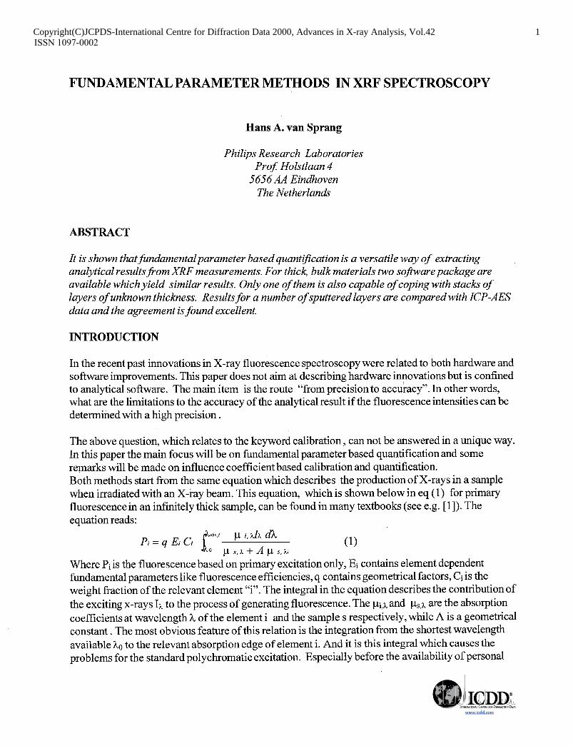
The analytical procedure used is straightforward. First the spectrometer was selected based on analytical criteria. In practice two Philips PW2400 spectrometers were available , one with a I& and one with a Cr anode x-ray tube. Only for the (Ag, In, Sb , Te) layers to be discussed below the Cr anode was preferred due to the bad efficiency of the Rh tube when exciting the L-lines of all of these elements. Subsequently standards were chosen. These standards were measured using the same analytical procedure and fluorescence lines as used for the “ unknowns “ later on. Subsequently the fluorescence intensities are calculated for the relevant elements. As an instrumental transmission factor PCFP W uses the ratio of the calculated over the measured intensity, while FP-WLTW uses the inverse. An example of a calibration plot as obtained from FP-MULTIW is shown in fig. 1 below. The slope of this line through the origin is used as a calibration coefficient. For unknown samples a “qualitative” model is made, describing the composition in terms of elements and , if relevant, the number of layers in combination with the elements per layer. PCFPW uses an internal procedure to generate adequate starting values to solve the set of equations. FP- MULTI requires a set of guessed starting values. Optimization stops when a specified criterion is fulfilled or a predefined number of iterations has been performed.


Figure 1 Calibration for Na as generated by FP-MULTI@‘.

The PCFPW and FP-MULTIW package have some features which are different. The most important are: l PCFPW supports batch processing of a number of similar samples l FP-MULTI@’ supports use with layered materials. l The algorithms describing the x-ray tube emission are different for both packages. l FP-MULTI requires an estimated sample composition as starting values for the optimization.


RESULTS FOR BULK MATERIALS OF INFINITE THICKNESS

A number of glass samples has been prepared for which the composition is well known. Some of the identifications refer to NIST standards. Four samples were used as calibration standards and the Na calibration plot in the introduction stems from this calibration procedure. The rest was used as if they were unknown samples containing the calibrated elements. . The results are summarized in table 1 below. The table requires some extra explanation.

All elements in the table are shown as weight fractions of the oxides although they are indicated using elementary symbols. The first 4 standards, 93a to G/4 were used as calibration standards. The selection criterion was the necessity to have all elements represented by at least 1 standard. . Due to the measurement procedure no backgrounds were measured for a number of elements. For these elements at least 2 points were needed. The indications in the column id refer to sample identities. Here 93a, 620 and 621 are NIST reference standards. The indications under org (origin) refer to the known composition (cer), the analytical result using PCFPW (pcf) or FPMULTI- W (fpw) The “0” indicates absence of a fluorescence signal for the relevant line.

In general the results show a very good correspondence for all elements. In a number of samples small quantities of other elements were also certified ( e.g. TiO$.These have been omitted intentionally but the quantification was always very accurate also for these minors. A further strong point is the automatic quantification of Boron. In all of the samples the amount of B2O3 was undefined at the start of the quantification. Because no fluorescence for B has been measured, the amount of B was determined as a kind of balance. This apparently works out reasonably well. A remark of caution applies to the results of PCFP W which does not use normalization to 100%. Quite often sums of concentrationexceed 100% and for comparison a manual normalization had to be performed. In order to quantify this type of samples using an influence coefficient method, all of these standards ( and even some more) had to be used to generate a calibration. When this procedure was replaced by a fundamental parameter procedure calibration time was reduced with a factor of 5. In addition the fundamental parameter procedure is easily adapted to additional elements because only one or a few standards containing this new element are sufficient to obtain an instrumental transmission factor for this element . Subsequently the unknown sample can be reliably quantified without requiring a full set of standards to correct for all third element effects as is needed in the case of influence coefficients.


Table I Composition of various glasses determined by FP quantification.

id 93a

js4

su8

G/4

621

ccl

r4

r5

r6

dgl

03

298

nnx

erg cer Pcf fPW cer Pcf fP w cer Pcf fP w cer Pcf fP w cer Pcf fPW cer Pcf fP w cer Pcf fP w cer PCf fP w cer Pc f fpw cer Pc f fP w cer Pcf fP w cer Pcf fPW cer Pc f fP w cer Pcf fpw cer Pcf fP w

B Na Mg Al 12.6 3.98 .Ol 2.3 13.0 3.32 0 2.3 12.3 4.01 0 2.3 2.5 8.24 .13 1.3 4.5 8.38 .06 1.2 2.7 8.51 .06 1.2 .59 11.0 .92 .86 .73 11.2 .92 1.0 0 11.2 .93 1.0 0 20.1 0 4.8 0.6 20.1 0 4.8 0 20.3 0 5.1 0 14.4 3.7 1.8 .19 14.6 3.8 1.8 0 14.7 3.9 1.8 0 12.7 .27 2.8 0 12.8 .24 2.8 0 13.0 .25 2.8 0 13.4 3.8 1.1 0 13.6 3.9 1.1 0 13.7 3.9 1.1 .19 15.4 0 1.7 .19 16.3 0 3.1 0 16.3 0 3.1 0 15.6 2.8 1.1 .54 15.8 2.8 1.0 0 16.0 2.9 1.0 0 14.6 0 1.7 I.23 14.7 0 1.6 0 14.9 0 1.6 0 14.9 4.1 1.2 0 15.0 4.4 1.2 0 15.2 4.4 1.2 0 13.7 3.4. .l 0 13.8 3.6 .l 0 14.1 3.6 0 0 16.6 2.9 1.5 0.2 16.4 3.0 1.5 0 16.5 3.0 1.5 18.4 1.14 .03 3.6 20.8 1.1 0 3.6 18.8 1.1 0 3.7 14.9 4.41 0 1.4 11.4 4.4 0 1.5 15.0 3.28 0 1.5

si Sb Ba Pb Fe Zn As Zr S K Ca 80.8 0 0 0 .03 0 0 .04 0 .Ol .Ol 81.2 0 .Ol 0 .02 .Ol 0 .04 0 .Ol .02 81.4 0 0 0 .02 0 0 .04 0 .Ol .02 67.6 0 3.8 0 .07 0 0 .03 .25 8.7 6.2 66.7 .04 37 0 .07 .Ol 0 .02 .25 8.7 6.3 68.1 .04 3.8 0 .07 0 0 .03 .25 8.9 6.4 69.5 .29 2.0 0 .02 0 .17 0 0 5.0 9.3 69.3 .29 2.1 0 .03 0 .07 0 .03 5.0 9.2 70.1 .30 2.1 0 .03 0 .06 0 .03 5.0 9.3 64.7 0 5.0 .83 0 2.9 .41 0 0 .05 0 64.1 0 5.0 .83 .03 2.9 .43 0 .03 .02 .02 66.5 0 5.4 34 0 3.0 .43 0 0 .02 .02 72.1 0 0 0 .04 0 .06 0 .28 .41 7.1 71.7 0 .02 0 .04 0 .03 .03 .23 .38 7.1 71.7 0 0 0 .04 0 .03 .03 .23 .38 7.2 71.1 0 .12 0 .04 0 .03 .Ol .13 2.0 10.7 70.7 0 .12 0 .03 0 .02 .Ol .lO 1.9 10.8 70.9 0 .13 0 .04 0 .02 .Ol .09 1.9 10.8 72.0 0 0 0 .lO 0 0 0 .22 .59 8.6 71.8 0 .03 0 .13 0 0 .Ol .19 .59 8.7 71.6 0 .03 0 .ll 0 0 .Ol .19 .59 8.8 73.1 0 0 0 .lO 3.3 0 0 0 .57 4.2 69.6 0 .06 .04 .12 3.0 .04 0 .08 .53 4.1 72.4 0 .06 .04 .ll 3.1 a .Ol .08 .54 4.3 72.7 0 0 0 .04 0 0 0 .21 .42 6.6 72.5 0 0 0 .04 .Ol .04 .03 .17 .40 6.5 72.8 0 .06 0 .04 .Ol .04 .03 .17 .40 6.6 73.1 0 0 0 .03 0 0 0 .2 0 9.9 71.8 0 .02 0 .02 0 .02 .Ol .16 .Ol 9.8 73.2 0 .02 0 .03 0 .02 .Ol .16 .Ol 9.9 71.7 0 0 0 .19 0 0 0 .44 .38 6.7 71.5 0 .02 0 .25 0 0 .Ol .35 .38 6.8 71.2 0 .02 0 .20 0 0 .Ol .35 .37 6.9 72.3 0 0 0 .02 0 0 0 .27 0 10.1 71.6 0 .02 0 0 0 0 0 .22 .02 10.1 71.7 0 .02 0 .Ol 0 0 0 .22 .02 10.2 69.5 .58 2.1 .38 .03 0 0 0 0 1.1 5.4 69.2 .71 2.0 .35 .03 0 .09 .Ol .03 1.1 5.5 69.1 .75 2.0 .35 .03 0 .09 .Ol .03 1.1 5.5 68.8 0 0 0 .04 0 0 .02 0 7.1 0 67.5 0 .04 0 .03 0 0 .Ol 0 6.8 .OS 69.1 0 .03 0 .03 0 0 .02 0 7.0 .08 73.2 0 .02 4.9 .04 0 .39 0 0 .71 0 75.7 0 .04 4.8 .03 0 1.3 .Ol 0 .73 .Ol 73.4 0 .04 4.7 .03 0 1.2 0 0 .68 .02


RESULTS FOR LAYERED MATERIALS OF UNKNOWN THICKNESS.

As can be understood from the introduction, the use of either an influence coefficient based calibration or the use of the PCFPW package is impossible for layered materials of unknown thickness. Nevertheless it is one of the main advantages of using Fp-based quantification that also quantificationof layered materials is possible. In the sections below a discussion will be given of two different types of layered samples which are routinely being analyzed using XRF in combination with FP-MULTIW. Both samples are layers of sputtered material used for optical recording. The first set contains Ge, Sb and Te as active components while the second series is concerned with In, Sb , Ag and Te. The first set, which contains Ge in addition to Sb and Te, has been measured on a PW2400 spectrometer equipped with a Rh tube. This mainly because Ge is minor constituent and for thin layers the Gel& is hardly observed when a Cr- anode tube is employed. For Sb and Sn the L-lines are being used and for these elements a Cr-anode tube would be preferred. The second series of layers, without the Ge, contains only elements for which a Cr- anode is more suitable, so these samples are measured on a spectrometer equipped with a Cr tube.

ANALYSIS OF THIN LAYERS OF GE, SB AND TE.

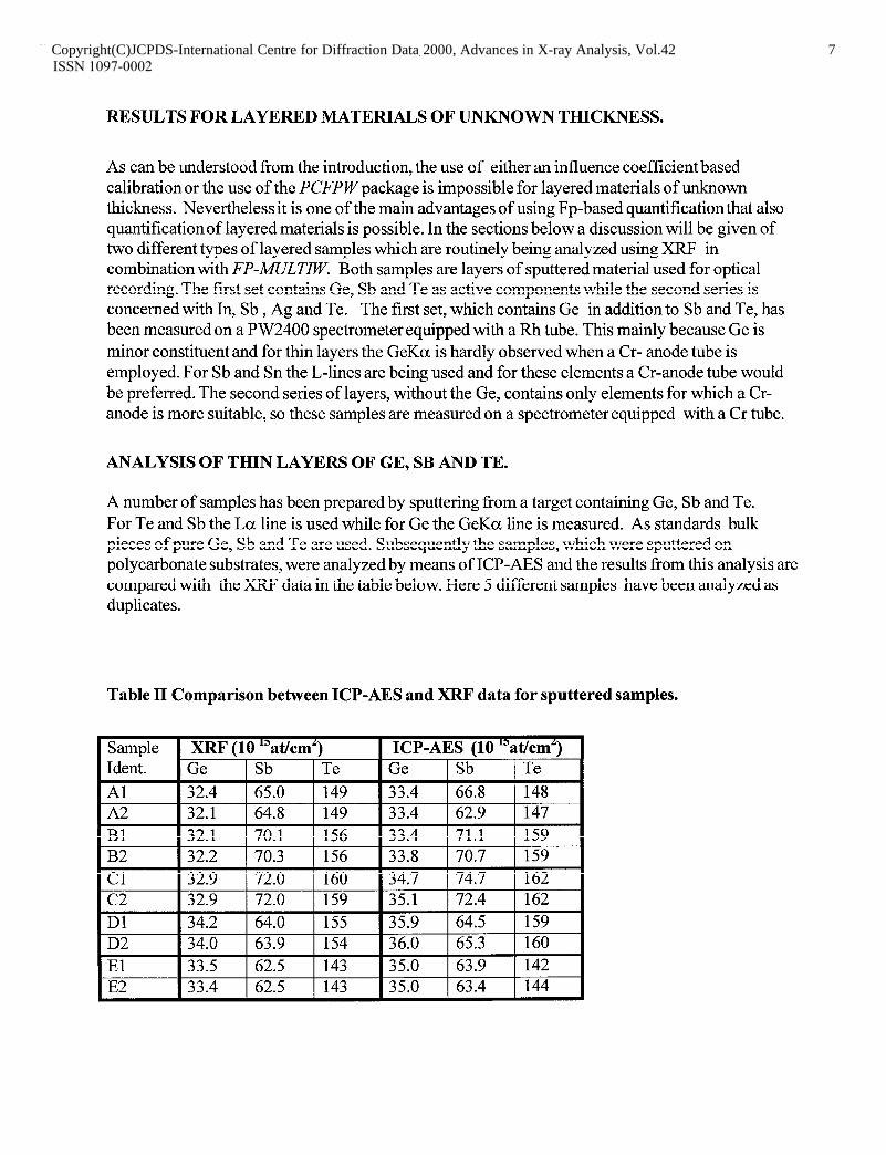
A number of samples has been prepared by sputtering from a target containing Ge, Sb and Te. For Te and Sb the La line is used while for Ge the GeKa line is measured. As standards bulk pieces of pure Ge, Sb and Te are used. Subsequently the samples, which were sputtered on polycarbonate substrates, were analyzed by means of ICP-AES and the results from this analysis are compared with the XRF data in the table below. Here 5 different samples have been analyzed as duplicates.

Table II Comparison between ICP-AES and XRF data for sputtered samples.

Sample Ident. Al A2 Bl B2 Cl c2 Dl D2 El E2

XRF (10 13at/cmL) Ge Sb Te 32.4 65.0 149 32.1 64.8 149 32.1 70.1 156 32.2 70.3 156 32.9 72.0 160 32.9 72.0 159 34.2 64.0 155

~ 34.0 63.9 154 33.5 62.5 143 33.4 62.5 143

ICP-AES (10 “at/cmL)

m

I I 33.4 I 71.1 I 159 33.8 70.7 159 34.7 74.7 162 35.1 72.4 162 35.9 64.5 159 36.0 65.3 160 I I 35.0 1 63.9 1 142 I I 35.0 1 63.4 I 144


As can be seen the results compare rather well. There are some differences but these are within the accuracies as claimed by both techniques. For ICP-AES this is generally said to be within 3% while for FP-MULTIW a 2-5% accuracy is found adequate. Because even for Ge the results match within 5%, we consider the agreement to be very good. This is even more encouraging because samples were used which were deposited on 3cm x 3cm square substrates. In XRF only a circular area of 2 cm diameter is being analyzed. So the borders of the sample are ignored in XRF while they are being used in the ICP analysis. For this reason part of the differences observed between both techniques could also be related to possible gradients in composition at the edges of the substrate.

LAYERED SAMPLES CONTAINING AG, IN, SB AND TE

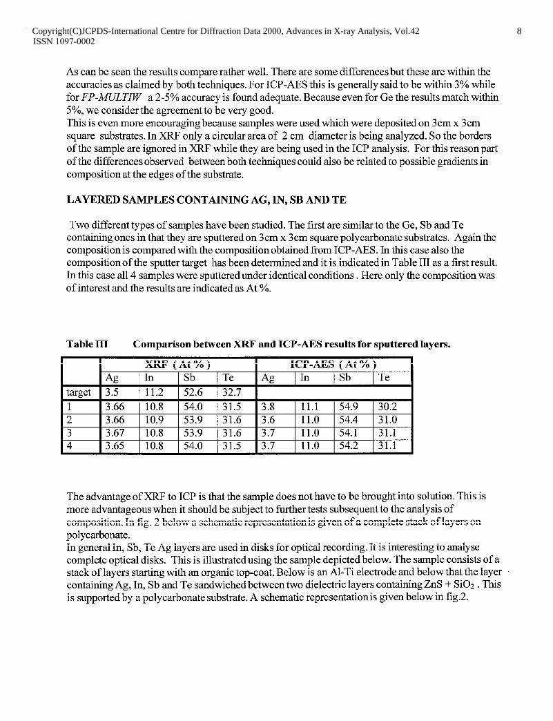
Two different types of samples have been studied. The first are similar to the Ge, Sb and Te containing ones in that they are sputtered on 3cm x 3cm square polycarbonate substrates. Again the composition is compared with the composition obtained from ICP-AES. In this case also the composition of the sputter target has been determined and it is indicated in Table III as a first result. In this case all 4 samples were sputtered under identical conditions . Here only the composition was of interest and the results are indicated as At %.

Table III Comparison between XRF and ICP-AES results for sputtered layers.

XRF (At%) Ag In Sb Te

target 3.5 11.2 52.6 32.7 1 3.66 10.8 54.0 31.5 2 3.66 10.9 53.9 31.6 3 3.67 10.8 53.9 31.6 4 3.65 10.8 54.0 31.5

ICP-AES ( At % ) 1 In 1 Sb 1 Te

3.8 11.1 54.9 30.2

I

3.6 11.0 54.4 31.0 3.7 11.0 54.1 31.1 3.7 11.0 54.2 31.1

The advantage of XRF to ICP is that the sample does not have to be brought into solution. This is more advantageous when it should be subject to further tests subsequent to the analysis of composition. In fig. 2 below a schematic representationis given of a complete stack of layers on polycarbonate. In general In, Sb, Te Ag layers are used in disks for optical recording. It is interesting to analyse complete optical disks. This is illustratedusing the sample depicted below. The sample consists of a stack of layers starting with an organic top-coat. Below is an Al-Ti electrode and below that the layer containing Ag, In, Sb and Te sandwiched between two dielectric layers containing ZnS + SiO2 . This is supported by a polycarbonate substrate. A schematic representationis given below in fig.2.


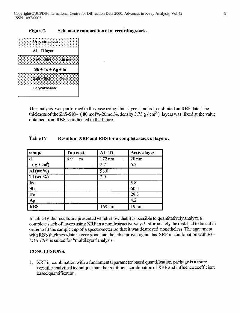
Figure 2 Schematic composition of a recording stack.

.:.:.:::: ‘.‘.‘.:.‘.‘.‘.‘.‘.:.:.:.:.:.: ,:i:;:::. :i~~~n?~?~P~~~:::::::::::: . . . . . . . . . . . . . . . . . . . . . . . . .~.~.~.~.~.~.~.~.

Al - Ti layer . . . . . . . . . . . . . . . . . . . . . . . . . . . . . . . . . . . . . . . . . . . . . . . . :i:i:i:i:i:i:i:i:i:~~~~~~~~~~~~~~~~~~~~~~~~~:~:~:~:~ . . . . . . . . . . . . . . . . . . . . . . . . . . . . :. . . . ::::. . . . . . . . . . . . . . . . . . . . . . . . . . . . . . . . . . . . . . . . v.......................................

Sb+Te+Ag+In

Polycarbonate

The analysis was performed in this case using thin-layer standards calibrated on RBS data. The thickness of the ZnS-Si02 ( 80 mol%-20mol%, density 3.73 g / cm3 ) layers was fixed at the value obtained from RIB as indicated in the figure.

Table IV Results of XRF and RBS for a complete stack of layers.

In table IV the results are presented which show that it is possible to quantitatively analyze a complete stack of layers using XRF in a nondestructive way. Unfortunately the disk had to be cut in order to fit the sample cup of a spectrometer, so that it was destroyed nonetheless. The agreement with RBS thickness data is very good and the table proves again that XRF in combination with FP- MULTIW is suited for “multilayer“ analysis.

CONCLUSIONS.

1. XRF in combination with a fundamental parameter based quantification package is a more versatile analytical technique than the traditional combination of XRF and influence coefficient based quantification.


2. For bulk materials of ( for XRP ) infinite thickness both the PCFP W and the FP-AKJLTIW software yield good results and allow for calibration using a small set of standards with easy extension to additional elements in “ unknown samples”

3. For layers and stacks of layers the FP-MULTIW package is a good choice. Comparison of the results with other techniques shows that XRF is a reliable and fast alternative to destructive, wet-chemical analysis.

REFERENCES.

1. R. Tertian and F.Claisse, Principles of Quantitative X-ray Spectroscopy, Heyden & son (1982) p56 - 69.

2. J. Sherman, Am. Sot. Tes. Mat. Spec. Tech. Publ. 157 (1954) 27 3. DKG de Boer and P.N. Brouwer, Adv. X-ray Analysis 33 (1990) 237. 4. P. Pella, L .Feng and J.A. Small, X-ray Spectrometry 14 (1985) 125 5. D.K.G. de Boer, J. J.M. Borstrok, A.J.G. Leenaers , H.A. van Sprang and P.N. Brouwer, X-ray

Spectrometry 22 (1993) 33

ACKNOWLEGMENT

The glass standards mentioned were prepared by Philips CFT. All XRF measurements were performed by Ms. T.J.M. Verspaget who also works at Philips CFT.


Fundamental Parameter Methods in XRF Spectroscopy · The basic theoretical treatment as used in...

Documents

Transcript of Fundamental Parameter Methods in XRF Spectroscopy · The basic theoretical treatment as used in...