Fundamental of communication engineering
668
-
Upload
wahli-nurdin -
Category
Engineering
-
view
75 -
download
4
Transcript of Fundamental of communication engineering


About the Author
Michael P. Fitz has experience both as a teacher of electrical communicationsand as a designer of electrical communication systems. He has been a profes-sor of electrical and computer engineering at the University of California LosAngeles (UCLA), the Ohio State University, and Purdue University. ProfessorFitz won the D. D. Ewing Undergraduate Teaching Award at Purdue Universityin 1995. Prof. Fitz was a member of the editorial board of the IEEE Transactionson Communications. Dr. Fitz has worked as a digital communication systemengineer for a variety of companies and currently is a senior communicationsystems engineer at Northrop Grumman. In these roles he has designed, built,and tested modems for land mobile and satellite communications applications.He received the 2001 IEEE Communications Society Leonard G. Abraham PrizePaper Award in the field of communications systems for his contributions tospace-time modem technology.
Copyright © 2007 by The McGraw-Hill Companies. Click here for terms of use.

Fundamentals ofCommunications
Systems
Michael P. Fitz
New York Chicago San FranciscoLisbon London Madrid Mexico City
Milan New Delhi San Juan SeoulSingapore Sydney Toronto

Copyright © 2007 by The McGraw-Hill Companies. All rights reserved. Manufactured in the United States of America. Except aspermitted under the United States Copyright Act of 1976, no part of this publication may be reproduced or distributed in any formor by any means, or stored in a database or retrieval system, without the prior written permission of the publisher.
0-07-151029-X
The material in this eBook also appears in the print version of this title: 0-07-148280-6.
All trademarks are trademarks of their respective owners. Rather than put a trademark symbol after every occurrence of a trade-marked name, we use names in an editorial fashion only, and to the benefit of the trademark owner, with no intention of infringe-ment of the trademark. Where such designations appear in this book, they have been printed with initial caps.
McGraw-Hill eBooks are available at special quantity discounts to use as premiums and sales promotions, or for use in corporatetraining programs. For more information, please contact George Hoare, Special Sales, at [email protected] or (212)904-4069.
TERMS OF USE
This is a copyrighted work and The McGraw-Hill Companies, Inc. (“McGraw-Hill”) and its licensors reserve all rights in and to thework. Use of this work is subject to these terms. Except as permitted under the Copyright Act of 1976 and the right to store andretrieve one copy of the work, you may not decompile, disassemble, reverse engineer, reproduce, modify, create derivative worksbased upon, transmit, distribute, disseminate, sell, publish or sublicense the work or any part of it without McGraw-Hill’s prior con-sent. You may use the work for your own noncommercial and personal use; any other use of the work is strictly prohibited. Yourright to use the work may be terminated if you fail to comply with these terms.
THE WORK IS PROVIDED “AS IS.” McGRAW-HILL AND ITS LICENSORS MAKE NO GUARANTEES OR WARRANTIESAS TO THE ACCURACY, ADEQUACY OR COMPLETENESS OF OR RESULTS TO BE OBTAINED FROM USING THEWORK, INCLUDING ANY INFORMATION THAT CAN BE ACCESSED THROUGH THE WORK VIA HYPERLINK OROTHERWISE, AND EXPRESSLY DISCLAIM ANY WARRANTY, EXPRESS OR IMPLIED, INCLUDING BUT NOT LIMIT-ED TO IMPLIED WARRANTIES OF MERCHANTABILITY OR FITNESS FOR A PARTICULAR PURPOSE. McGraw-Hill andits licensors do not warrant or guarantee that the functions contained in the work will meet your requirements or that its operationwill be uninterrupted or error free. Neither McGraw-Hill nor its licensors shall be liable to you or anyone else for any inaccuracy,error or omission, regardless of cause, in the work or for any damages resulting therefrom. McGraw-Hill has no responsibility forthe content of any information accessed through the work. Under no circumstances shall McGraw-Hill and/or its licensors be liablefor any indirect, incidental, special, punitive, consequential or similar damages that result from the use of or inability to use thework, even if any of them has been advised of the possibility of such damages. This limitation of liability shall apply to any claimor cause whatsoever whether such claim or cause arises in contract, tort or otherwise.
DOI: 10.1036/0071482806

We hope you enjoy thisMcGraw-Hill eBook! If
you’d like more information about this book,its author, or related books and websites,please click here.
Professional
Want to learn more?

This book is dedicated to
■ the memory of my parents. If my children become half the human beings thatmy siblings are, I will consider myself a success in life.
■ Mary. She has given up much to let me pursue my follies. I hope I can nowgive back to her in an equal amount!

This page intentionally left blank

Contents
Preface xvAcknowledgements xxxi
Chapter 1 Introduction 1.1
1.1 Historical Perspectives on Communication Theory 1.11.2 Goals for This Text 1.31.3 Modern Communication System Engineering 1.41.4 Technology’s Impact on This Text 1.61.5 Book Overview 1.7
1.5.1 Mathematical Foundations 1.71.5.2 Analog Communication 1.81.5.3 Noise in Communication Systems 1.91.5.4 Fundamentals of Digital Communication 1.10
1.6 Homework Problems 1.10
PART 1 MATHEMATICAL FOUNDATIONS
Chapter 2 Signals and Systems Review 2.1
2.1 Signal Classification 2.12.1.1 Energy versus Power Signals 2.12.1.2 Periodic versus Aperiodic 2.42.1.3 Real versus Complex Signals 2.52.1.4 Continuous Time Signals versus Discrete Time Signals 2.6
2.2 Frequency Domain Characterization of Signals 2.62.2.1 Fourier Series 2.62.2.2 Fourier Transform 2.92.2.3 Bandwidth of Signals 2.142.2.4 Fourier Transform Representation of Periodic Signals 2.162.2.5 Laplace Transforms 2.18
2.3 Linear Time-Invariant Systems 2.18
vii
For more information about this title, click here

viii Contents
2.4 Utilizing Matlab 2.232.4.1 Sampling 2.232.4.2 Integration 2.242.4.3 Commonly Used Functions 2.24
2.5 Homework Problems 2.252.6 Example Solutions 2.332.7 Miniprojects 2.36
2.7.1 Project 1 2.362.7.2 Project 2 2.37
Chapter 3 Review of Probability and Random Variables 3.1
3.1 Axiomatic Definitions of Probability 3.13.2 Random Variables 3.6
3.2.1 Cumulative Distribution Function 3.63.2.2 Probability Density Function 3.83.2.3 Moments and Statistical Averages 3.93.2.4 The Gaussian Random Variable 3.103.2.5 A Transformation of a Random Variable 3.12
3.3 Multiple Random Variables 3.143.3.1 Joint Density and Distribution Functions 3.143.3.2 Joint Moments and Statistical Averages 3.163.3.3 Two Gaussian Random Variables 3.163.3.4 Transformations of Random Variables 3.193.3.5 Central Limit Theorem 3.213.3.6 Multiple Dimensional Gaussian Random Variables 3.22
3.4 Homework Problems 3.233.5 Example Solutions 3.333.6 Miniprojects 3.36
3.6.1 Project 1 3.36
Chapter 4 Complex Baseband Representation of Bandpass Signals 4.1
4.1 Introduction 4.14.2 Baseband Representation of Bandpass Signals 4.24.3 Visualization of Complex Envelopes 4.64.4 Spectral Characteristics of the Complex Envelope 4.9
4.4.1 Basics 4.94.4.2 Bandwidth of Bandpass Signals 4.13
4.5 Power of Carrier Modulated Signals 4.144.6 Linear Systems and Bandpass Signals 4.144.7 Conclusions 4.184.8 Homework Problems 4.184.9 Example Solutions 4.30
4.10 Miniprojects 4.334.10.1 Project 1 4.334.10.2 Project 2 4.33

Contents ix
PART 2 ANALOG COMMUNICATION
Chapter 5 Analog Communications Basics 5.1
5.1 Message Signal Characterization 5.15.2 Analog Transmission 5.5
5.2.1 Analog Modulation 5.65.2.2 Analog Demodulation 5.6
5.3 Performance Metrics for Analog Communication 5.85.4 Preview of Pedagogy 5.115.5 Homework Problems 5.125.6 Example Solutions 5.15
Chapter 6 Amplitude Modulation 6.1
6.1 Linear Modulation 6.16.1.1 Modulator and Demodulator 6.56.1.2 Coherent Demodulation 6.66.1.3 DSB-AM Conclusions 6.8
6.2 Affine Modulation 6.86.2.1 Modulator and Demodulator 6.126.2.2 LC-AM Conclusions 6.16
6.3 Quadrature Modulations 6.166.3.1 VSB Filter Design 6.176.3.2 Single Sideband AM 6.196.3.3 Modulator and Demodulator 6.226.3.4 Transmitted Reference Based Demodulation 6.236.3.5 Quadrature Modulation Conclusions 6.27
6.4 Homework Problems 6.276.5 Example Solutions 6.426.6 Miniprojects 6.44
6.6.1 Project 1 6.456.6.2 Project 2 6.456.6.3 Project 3 6.46
Chapter 7 Analog Angle Modulation 7.1
7.1 Angle Modulation 7.17.1.1 Angle Modulators 7.6
7.2 Spectral Characteristics 7.77.2.1 A Sinusoidal Message Signal 7.77.2.2 General Results 7.14
7.3 Demodulation of Angle Modulations 7.197.4 Comparison of Analog Modulation Techniques 7.247.5 Homework Problems 7.257.6 Example Solutions 7.377.7 Miniprojects 7.39
7.7.1 Project 1 7.397.7.2 Project 2 7.40

x Contents
Chapter 8 More Topics in Analog Communications 8.1
8.1 Phase-Locked Loops 8.18.1.1 General Concepts 8.18.1.2 PLL Linear Model 8.4
8.2 PLL–Based Angle Demodulation 8.48.2.1 General Concepts 8.48.2.2 PLL Linear Model 8.6
8.3 Multiplexing Analog Signals 8.88.3.1 Quadrature Carrier Multiplexing 8.98.3.2 Frequency Division Multiplexing 8.10
8.4 Conclusions 8.138.5 Homework Problems 8.138.6 Example Solutions 8.198.7 Miniprojects 8.20
8.7.1 Project 1 8.20
PART 3 NOISE IN COMMUNICATIONS SYSTEMS
Chapter 9 Random Processes 9.1
9.1 Basic Definitions 9.29.2 Gaussian Random Processes 9.59.3 Stationary Random Processes 9.9
9.3.1 Basics 9.109.3.2 Gaussian Processes 9.119.3.3 Frequency Domain Representation 9.15
9.4 Thermal Noise 9.199.5 Linear Systems and Random Processes 9.239.6 The Solution of the Canonical Problem 9.279.7 Homework Problems 9.309.8 Example Solutions 9.429.9 Miniprojects 9.44
9.9.1 Project 1 9.449.9.2 Project 2 9.44
Chapter 10 Noise in Bandpass Communication Systems 10.110.1 Bandpass Random Processes 10.410.2 Characteristics of the Complex Envelope 10.6
10.2.1 Three Important Results 10.610.2.2 Important Corollaries 10.9
10.3 Spectral Characteristics 10.1210.4 The Solution of the Canonical Bandpass Problem 10.1510.5 Complex Additive White Gaussian Noise 10.1810.6 Conclusion 10.1910.7 Homework Problems 10.1910.8 Example Solutions 10.2710.9 Miniprojects 10.29
10.9.1 Project 1 10.30

Contents xi
Chapter 11 Fidelity in Analog Demodulation 11.111.1 Unmodulated Signals 11.111.2 Bandpass Demodulation 11.4
11.2.1 Coherent Demodulation 11.511.3 Coherent Amplitude Demodulation 11.6
11.3.1 Coherent Demodulation 11.611.4 Noncoherent Amplitude Demodulation 11.911.5 Angle Demodulations 11.12
11.5.1 Phase Modulation 11.1211.5.2 Frequency Modulation 11.15
11.6 Improving Fidelity with Pre-Emphasis 11.1711.7 Final Comparisons 11.1911.8 Homework Problems 11.2011.9 Example Solutions 11.26
11.10 Miniprojects 11.2911.10.1 Project 1 11.2911.10.2 Project 2 11.29
PART 4 FUNDAMENTALS OF DIGITAL COMMUNICATION
Chapter 12 Digital Communication Basics 12.112.1 Digital Transmission 12.2
12.1.1 Digital Modulation 12.212.1.2 Digital Demodulation 12.3
12.2 Performance Metrics for Digital Communication 12.412.2.1 Fidelity 12.412.2.2 Complexity 12.512.2.3 Bandwidth Efficiency 12.612.2.4 Other Important Characteristics 12.7
12.3 Some Limits on Performance of Digital Communication Systems 12.812.4 Conclusion 12.1012.5 Homework Problems 12.1112.6 Example Solutions 12.1412.7 Miniprojects 12.14
12.7.1 Project 1 12.15
Chapter 13 Optimal Single Bit Demodulation Structures 13.113.1 Introduction 13.1
13.1.1 Statistical Hypothesis Testing 13.313.1.2 Statistical Hypothesis Testing in Digital Communications 13.513.1.3 Digital Communications Design Problem 13.6
13.2 Minimum Probability of Error Bit Demodulation 13.713.2.1 Characterizing the Filter Output 13.913.2.2 Uniform A Priori Probability 13.11
13.3 Analysis of Demodulation Fidelity 13.1413.3.1 Erf Function 13.1513.3.2 Uniform A Priori Probability 13.16
13.4 Filter Design 13.1813.4.1 Maximizing Effective SNR 13.1813.4.2 The Matched Filter 13.20

xii Contents
13.4.3 MLBD with the Matched Filter 13.2113.4.4 More Insights on the Matched Filter 13.23
13.5 Signal Design 13.2513.6 Spectral Characteristics 13.2813.7 Examples 13.30
13.7.1 Frequency Shift Keying 13.3013.7.2 Phase Shift Keying 13.3613.7.3 Discussion 13.39
13.8 Homework Problems 13.4013.9 Example Solutions 13.50
13.10 Miniprojects 13.5513.10.1 Project 1 13.5513.10.2 Project 2 13.57
Chapter 14 Transmitting More Than One Bit 14.114.1 A Reformulation for 1 Bit Transmission 14.114.2 Optimum Demodulation 14.3
14.2.1 Optimum Word Demodulation Receivers 14.414.2.2 Analysis of Demodulation Fidelity 14.714.2.3 Union Bound 14.1014.2.4 Signal Design 14.16
14.3 Examples 14.1714.3.1 M-ary FSK 14.1714.3.2 M-ary PSK 14.2114.3.3 Discussion 14.26
14.4 Homework Problems 14.2714.5 Example Solutions 14.3714.6 Miniprojects 14.40
14.6.1 Project 1 14.41
Chapter 15 Managing the Complexity of Optimum Demodulation 15.115.1 Linear Modulations 15.2
15.1.1 MLWD for Linear Modulation 15.315.1.2 Error Rate Evaluation for Linear Modulation 15.615.1.3 Spectral Characteristics of Linear Modulation 15.1015.1.4 Example: Square Quadrature Amplitude Modulation 15.1015.1.5 Summary of Linear Modulation 15.10
15.2 Orthogonal Modulations 15.1315.3 Orthogonal Modulation Examples 15.16
15.3.1 Orthogonal Frequency Division Multiplexing 15.1615.3.2 Orthogonal Code Division Multiplexing 15.2215.3.3 Binary Stream Modulation 15.26
15.4 Conclusions 15.3015.5 Homework Problems 15.3115.6 Example Solutions 15.4815.7 Miniprojects 15.53
15.7.1 Project 1 15.5415.7.2 Project 2 15.5415.7.3 Project 3 15.54

Contents xiii
Chapter 16 Spectrally Efficient Data Transmission 16.116.1 Spectral Containment 16.116.2 Squared Cosine Pulse 16.316.3 Spectral Shaping in OFDM 16.516.4 Spectral Shaping in Linear Stream Modulations 16.716.5 Testing Orthogonal Modulations 16.11
16.5.1 The Scatter Plot 16.1216.5.2 Stream Modulations 16.15
16.6 Conclusions 16.1816.7 Homework Problems 16.1816.8 Example Solutions 16.2216.9 Miniprojects 16.23
16.9.1 Project 1 16.2316.9.2 Project 2 16.2516.9.3 Project 3 16.2616.9.4 Project 4 16.27
Chapter 17 Orthogonal Modulations with Memory 17.117.1 Canonical Problems 17.117.2 Orthogonal Modulations with Memory 17.2
17.2.1 MLWD for Orthogonal Modulations with Memory 17.417.2.2 An Example OMWM Providing Better Fidelity 17.517.2.3 Discussion 17.7
17.3 Spectral Characteristics of Stream OMWM 17.917.3.1 An Example OMWM with a Modified Spectrum 17.917.3.2 Spectrum of OMWM for Large Kb 17.11
17.4 Varying Transmission Rates with OMWM 17.1617.4.1 Spectrum of Stream Modulations with Nm > 1 17.1717.4.2 Example R < 1: Convolutional Codes 17.2117.4.3 Example R > 1: Trellis Codes 17.2317.4.4 Example for Spectral Shaping: Miller Code 17.26
17.5 Conclusions 17.2817.6 Homework Problems 17.3017.7 Example Solutions 17.3617.8 Miniprojects 17.37
17.8.1 Project 1 17.39
Appendix A Useful Formulas A.1
Appendix B Notation B.1
Appendix C Acronyms C.1
Appendix D Fourier Transforms: f versus ω D.1
Appendix E Further Reading and Bibliography E.1
Index I.1

This page intentionally left blank

Preface
My goal in teaching communications (and in authoring this text) is to providestudents with
■ an exposition of the theory required to build modern communication systems.■ an insight into the required trade-offs between spectral efficiency of trans-
mission, fidelity of message reconstruction, and complexity of system imple-mentation that are required for a modern communication system design.
■ a demonstration of the utility and applicability of the theory in the homeworkproblems and projects.
■ a logical progression in thinking about communication theory.
Consequently, this textbook will be more mathematical than most and does notdiscuss examples of communication systems except as a way to illustrate howimportant communication theory concepts solve real engineering problems. Myexperience has been that my approach works well in an elective class wherestudents are interested in communication careers or as a self-study guide tocommunications. My approach does not work as well when the class is a requiredcourse for all electrical engineering students as students are less likely to seethe advantage of developing tools they will not be using in their career. Matlabis used extensively to illustrate the concepts of communication theory as it isa great visualization tool and probably the most prevalent system engineeringtool used in practice today. To me the beauty of communication theory is thelogical flow of ideas. I have tried to capture this progression in this text. Onlyyou the reader will be able to decide how I have done in this quest.
Teaching from This Text
This book is written for the modern communications curriculum. The courseobjectives for an undergraduate communication course that can be taught fromthis text are (along with their ABET criteria)
■ Students learn the bandpass representation for carrier modulated signals.(Criterion 3(a))
xv
Copyright © 2007 by The McGraw-Hill Companies. Click here for terms of use.
xvi Preface
■ Students engage in engineering design of communications system compo-nents. (Criteria 3(c),(k))
■ Students learn to analyze the performance, spectral efficiency and complexityof the various options for transmitting analog and digital message signals.(Criteria 3(e),(k))
■ Students learn to characterize noise in communication systems. (Criterion3(a))
Prerequisites to this course are probability and random variables and a signaland systems course.
I have taught out of this book material in several ways. I have been luckyto teach at three universities (Purdue University, the Ohio State University,and the University of California Los Angeles) and each of these experienceshas profoundly impacted my writing of this book. The material in this book hasbeen used to teach three classes
■ Undergraduate analog communications and noise (30 lecture hours)■ Undergraduate digital communications (30 lecture hours)■ Undergradute communications (40–45 lecture hours)
The course outline for the 30 lecture hours of analog communication is
1. Chapters 1 & 2 — 1 hour. This lecture was a review of a previous class.
2. Chapter 4 — 2 hours. These lectures build heavily on signal and systemtheory and specifically the frequency translation theorem of the Fouriertransform.
3. Chapter 5 — 1 hour. This lecture introduces the concept of analog modu-lation and the performance metrics that engineers use in designing analogcommunication systems.
4. Chapter 6 — 5 hours. These lectures introduce amplitude modulation anddemodulation algorithms. Since this course was an analog only course, Ispend more time on the practical demodulation structures for DSB-AMand VSB-AM.
5. Chapter 7 — 5 hours. These lectures introduce angle modulation and de-modulation algorithms. I like to emphasize that the understanding of thespectrum of angle modulations is best facilitated by the use of the Fourierseries.
6. Chapter 8 — 2 hours. These lectures introduce multiplexing and the phase-locked loop. Multiplexing is an easy concept and yet students enjoy it be-cause of the practical examples that can be developed.
7. Chapters 3 & 9 — 6 hours. These lectures introduce random variables andrandom processes. This, from the student’s perspective, is the most difficult

Preface xvii
part of the class as the concept of noise and random processes are mathe-matically abstract. Undergraduates are not used to abstract concepts beingimportant in practice.
8. Chapter 10 — 3 hours. These lectures introduce bandpass random pro-cesses. This goes fairly well once Chapter 9 has been swallowed.
9. Chapter 11 — 3 hours. These lectures introduce fidelity analysis and theresulting SNR for each of the modulation types that have been introduced.The payoff for all the hard work to understand random processes.
10. Test — 1 hour.
The 30 hour digital only communication course followed the analog course soit could build on the material in the previous course. This course often containedsome graduate students from outside the communications field that sat in onthe course so some review was necessary. The course outline for 30 lecture hoursof digital communications is
1. Chapter 1 & 4 — 2 hours. These lectures introduce communications andbandpass signals.
2. Chapter 9 & 10 — 2 hours. These lectures introduce noise and noise incommunication systems.
3. Chapter 12 — 1 hour. This lecture introduces the concept of digital modula-tion and the performance metrics that engineers use in designing systems.This lecture also introduces Shannon’s limits in digital communications.
4. Chapter 13 — 6 hours. These lectures emphasize the five-step design processinherent in digital communications. In the end these lectures show how farsingle-bit transmission is from Shannon’s limit.
5. Chapter 14 — 4 hours. These lectures show how to extend the single bitconcepts to M-ary modulation. These lectures show how to achieve differentperformance-spectral efficiency trade-offs and how to approach Shannon’slimit.
6. Chapter 15 — 8 hours. These lectures introduce most of the modulationformats used in engineering practice by examing the complexity associatedwith demodulation.
7. Chapter 16 — 3 hours. These lectures introduce bandwidth efficient trans-mission and tools used to test digital communication systems.
8. Chapter 17 — 2 hours. These lectures introduce coded modulations as a wayto reach Shannon’s bounds.
9. Test — 1 hour.
The 40–45 hour analog and digital communication course I taught tradition-ally had a much more aggressive schedule. The course outline for 40 lecturehours of communications is

xviii Preface
1. Chapters 1 & 2 — 1 hour. The signal and systems topics were a review of aprevious class.
2. Chapter 4 — 2 hours. These lectures build heavily on Fourier transformtheory and the frequency translation theorem of the Fourier transform.
3. Chapter 5 — 1 hour. This lecture introduces the concept of analog modula-tion and the performance metrics that engineers use in designing systems.
4. Chapter 6 — 4 hours. These lectures introduce amplitude modulation anddemodulation algorithms. The focus of the presentation was limited to co-herent demodulators and the envelope detector.
5. Chapter 7 — 4.5 hours. These lectures introduce angle modulation anddemodulation algorithms. I like to emphasize that the understanding of thespectrum of angle modulations is best facilitated by the use of the Fourierseries.
6. Chapter 8 — 0.5 hour. Only covered multiplexing.
7. Chapters 3 & 9 — 5 hours. This is the toughest part of the class as theconcept of noise and random processes are mathematically abstract. Un-dergraduates are not used to abstract concepts being important in practice.
8. Chapter 10 — 2 hours. This goes fairly well once Chapter 9 has been swal-lowed.
9. Chapter 11 — 2 hours. The payoff for all the hard work to understandrandom processes.
10. Chapter 12 — 1 hour. This lecture introduces the concept of digital modula-tion and the performance metrics that engineers use in designing systems.This lecture also introduces Shannon’s limits in digital communications.
11. Chapter 13 — 6 hours. These lectures emphasize the five-step design pro-cess inherent in digital communications. In the end these lectures showhow far single-bit transmission is from Shannon’s limit.
12. Chapter 14 — 4 hours. These lectures show how to extend the single bitconcepts to M-ary modulation. These lectures show how to achieve differentperformance-spectral efficiency trade-offs and how to approach Shannon’slimit.
13. Chapter 15 — 3 hours. These lectures introduce most of the modulationformats used in engineering practice by examing the complexity associatedwith demodulation.
14. Chapter 16 — 1 hours. These lectures introduce bandwidth efficient trans-mission and tools used to test digital communication systems.
15. Chapter 17 — 1 hours. These lectures introduce coded modulations as away to reach Shannon’s bounds.
16. Test — 1 hour.
The 45 hour course added more details in the digital portion of the course.

Preface xix
Style Issues
This book takes a stylistic approach that is different than the typical commu-nication text. A few comments are worth making to motivate this style.
Property–Proof
One stylistic technique that I adopted in many of the sections, especially wheretools for communication theory are developed, was the use of a property state-ment followed by a proof. There are two reasons why I choose this approach
1. The major result is highlighted clearly in the property statement. Students,in a first pass, can understand the flow of the development without gettingbogged down in the details. I have found that this flow is consistent withstudent (and my) learning patterns.
2. Undergraduate students are increasingly not well trained in logical thinkingin regard to engineering concepts. The proofs give them some flavor for theprocess of logical thinking in engineering systems.
General Concepts Followed by Practical Examples
My approach is to teach general concepts and then follow up with specific ex-amples. To me the most important result from a class taught from this bookis the learning of fundamental tools. I emphasize these tools by making themthe focus of the book. Students entering the later stages of their engineeringeducation want to see that the hard work they have put into an engineeringeducation has practical benefits. The course taught from this book is really funfor the students as old tools (signals and systems and probability) and newlydeveloped tools are needed to understand electronic communication.
Two Types of Homework Problems
This book contains two types of homework problems: (1) direct applicationproblems and (2) extension problems. The application problems try to definea problem that is a straightforward application of the material developed inthe text. The extension problem requires the student to think “outside the box”and extend the theory learned in class to cover other important topics or coverpractical applications. As a warning to students and professors: Often timesthe direct application problems will appear ridiculously simple if you carefullyread the text and the extension problems, as they are often realistic engineer-ing problems, appear to be much too extensive for a homework problem. I havefound that both types of problems are important for undergraduate education.Direct application problems allow you to practice the theory but are usually notindicative of the types of problems an engineer sees in practice. Alternativelystudents often desire realistic problems as they want a feel for “real” engineer-ing but often get overwhelmed with the details needed in realistic problems. Alldirect application leads to a boring sterile course and all extension problemsdiscourage all but the exceptionally smart and motivated. Having a book with

xx Preface
both types of problems allows the student to both exercise and extend theirlearning in the proper balance.
Examples and Example Solutions
My learning style is one where a very succinct presentation of the issues worksbest. I originally wrote this book where the material was presented in a con-densed version with little or no examples. I then followed each chapter with aset of example solutions to homework problems. During the many revisions ofthe book I came to realize that many students learn best with examples alongwith a presentation of the theory. I added a significant number of in-text exam-ples to meet this learning need. I still like a succinct presentation so I did notmove all example solutions to in chapter examples. Consequently, each chapterhas a set of in-chapter examples and a set of worked solutions. This method wasviewed as a compromise between a succinct presentation (my learning style andhopefully a few others) and lots of examples (many students’ learning style).
Miniprojects
Both for myself and the students I have taught, learning is consumated in“doing.” I include “Miniprojects” in the book to give the students a chance toimplement the theory. The project solutions are appropriate for oral presenta-tion and this gives the students experience that will be a valuable part of anengineering career. The format of the project is such that it is most easily donein Matlab as that is the most common computer tool used in communicationengineering systems. To aid students who are not familiar with Matlab pro-gramming I have included the code for all the Matlab generated figures in thetext on the book web page. This also allows students to see how the theory canbe implemented in practice.
Writing of the Book
The big question that has to be answered in this preface is “Why should anyonewrite another communication theory book?” The short answer is “There is nogood reason for the book and a rational person would not have written the book.”The book resulted from a variety of random decisions and my general enjoymentof communication engineering. A further understanding of this book and mydecision to write it can be obtained by understanding the stages I perceivedin looking back on the writing this book. This documentation is done in somesense for those who will follow in my folly of attempting to write a book to givethem a sense of the journey.
1. Captured. As a child, a high school student and a college student I wasalways drawn to math and science, to problem solving, and to challenges.Quickly my career path steered toward engineering, toward electrical en-gineering, and finally toward communication engineering. I took a job as acommunication engineer while pursuing a graduate education. In the first

Preface xxi
four years of working I used all of my graduate classes in solving communi-cation problems and was a key engineer in a team that built and field testeda sophisticated wireless modem. I was hooked by communications engineer-ing: It is a field that has a constant source of problems, a well-defined set ofmetrics to be used in problem solving, and a clear upperbound (due to ClaudeShannon) to which each communication system could aspire.
2. Arrogance. I started my academic career, after being reasonably success-ful while working in industry, with the feeling that I knew a great deal. Iwas convinced that my way of looking at communications was the best and Istarted teaching as such. I found the textbooks available at the time to haveinadequate coverage of the complex envelope representation of bandpass sig-nals and bandpass noise and other modern topics. Hence my writing careerstarted by preparing handouts for my classes on these topics. I quickly gotup to 100 pages of material.
3. Humbled but Learning. It was not too long after starting to teach anddirect graduate student research that I came to the realization that the fieldof communications was a mighty river and I had explored only a few fairlyminor tributaries. I came to realize I did not know much and still needed tolearn much. This realization began to be reflected in my teaching as well. Ibranched out and learned other fields and reflected my new understanding inmy teaching methods and approaches. Much to my students’ chagrin, I oftenused teaching as a method to explore the boundaries of my own learning. Thisresulted in many poorly constructed homework problems and lectures thatwere rough around the edges. As I am not very bright, when I synthesizedmaterial I always had to put it into my own notation to keep things clear inmy own mind. After these bouts with new material that were very confusingfor my students, I often felt guilty and wrote up notes to clarify my ramblings.Soon I was up to 200 pages of material on digital communications. As I woulddiscover later these notes, while technically correct, were agonizingly brieffor students and lacked sufficient examples to aid in learning.
4. Cruise Control. I soon got to the point where I had reasonable notes andhomework and my family and professional committments had grown to thepoint where I needed not to focus so much on my teaching and let things runa bit in cruise control. During this time I added a lot of homework and testproblems and continued to write up and edit material that was confusing tostudents. My research always seems filled with interesting side issues thatmake great homework problems. I started the practice of keeping a note bookof issues that have come up during research and then tried to morph theseissues into useful homework problems. Some problems were successes andsome were not. In 2002, I was up to about 300 pages.
5. Well I have 300 Pages . . . At the point of 300 pages I felt like I turned acorner and had a book almost done and started shopping this book aroundto publishers. My feeling was that there was not much left to complete andonce I signed a contract the book would appear in 6 months. This writing

xxii Preface
would magically take place while my professional and family life flourished.I eagerly wrote more material and was up to 400 pages.
6. . . . And Then Depression Set In. When I looked at my project with thecritical eye produced by signing a contract, it quickly became apparent thatlots of pages do not necessarily equate to a book of any quality. At this timeI also got my first reviews back on the book and quickly came to realizewhy all textbooks on communications look the same to me. If you took theunion of the reviews you would end up with a book close to all the bookson the market (that I obviously did not fully appreciate). During this time Istruggled mightily at trying to smooth out the rough edges of the book andaddress reviewers’ concerns, while trying to keep what I thought was mypersonal perspective on communications. This was a significant struggle forme, as I learned the difficult lesson that each person is unique in how theyperceive the world and consequently in what they want in a textbook but Istubbornly soldiered through to completion.
In summary the book resulted not from a well thought out plan but from twodisjointed themes: (1) my passionate enjoyment of communication engineering,(2) my constant naive thinking as a professional. The book is done and it ismuch different than I first imagined it. It is unique in its perspective but notnecessarily markedly different than the other books out there. It is time torelease my creation.
Heresies in the Book
The two things I learned in writing this book is that engineering professionalsdo not see the field the same and engineering professors do not like change.In trying to tell my version of the communication story I thought long andhard about how to make the most consistent and compelling story of commu-nication engineering for my students. In spite of what I considered a carefullyconstructed pedagogy, I have been accused (among other things) of making upnomenclature and confusing the student needlessly. Since I now realize thatI am guilty of several potential heresies to the field of communication educa-tion, I decided to state these heresies clearly in the preface so all (especiallythose that teach from this book) know my positions (and structure their classesappropriately).
1. System Engineering Approach. I have worked as a communication en-gineer in industry and academia. I do not have a detailed knowledge ofcircuit theory and yet from all outward appearances I have thrived in myprofession by only being an expert in system modeling and analysis. Thistext will not give circuits to build communication systems as circuits willchange over time but will discuss mathematical concepts as these are con-sistent over time. I am a firm believer that communications engineering isperhaps unique in how theory directly gets implemented in practice.

Preface xxiii
2. Fidelity, Complexity, and Spectral Efficiency. Everything in electroniccommunications engineering comes down to a trade-off between fidelity ofmessage reconstruction, complexity/cost of the electronic systems used toimplement this communication, and the spectral efficiency of the transmis-sion. I have decided to adopt this approach in my teaching. This approachclearly deviates from past practice and has not proven to be universallypopular.
3. Stationary versus Wide-Sense Stationary. An interesting characteris-tic in my education was that a big deal was made out of the difference be-tween stationary and wide-sense stationary random processes – and mostlikely for all communication engineers of my generation. As I went throughmy life as a communication engineering professional I came to the real-ization that this additional level of abstraction was only needed becausethe concept of stationarity was arbitrarily introduced before the concept ofGaussianity. For my book, I introduce Gaussian processes first and then theidea of wide-sense stationarity is never needed. My view is clearly not ap-preciated by all1 but my book has only stationary Gaussian processes andrandom variables. I felt the less new concepts in random processes thatare introduced in teaching students how to analyze the fidelity of messagereconstruction, the better the student learning experience would be.
4. Information Theory Bounds. My view is that digital communication isan exciting field to work in because there are some bounds to motivate whatwe do. Claude Shannon introduced a bound on the achievable fidelity andspectral efficiency in the 1940s [Sha48]. Communication engineers havebeen pursuing how to achieve these bounds in a reasonable complexityever since. Many people feel strongly that Shannon’s bounds cannot beintroduced to undergraduates and I disagree with that notion! It is arguablethat Claude Shannon has a bigger impact on modern life than does AlbertEinstein yet name recognition among engineering and science studentsis not high for Claude Shannon. Hopefully introducing Shannon and hisbounds to undergraduates can give him part of his due.
5. Erfc(•) versus Q(•). The tail probability of a Gaussian random variablecomes up frequently in digital communications. The tail probability of aGaussian random variable is not given by a simple expression but insteadmust be evaluated numerically. Past authors have used three different tran-scendental functions to specify tail probabilities: Erfc(•), �(•), and the Q(•).Historically, communication engineers have gravitated to the use of Q(•) asits definition matches more closely how the usage comes up in digital com-munications. I have chosen to buck this trend because of one simple fact:Matlab is the most common tool used in modern communications engineer-ing and Matlab uses Erfc(•). Most people who read this text after having
1Some reviewers went so far as to suggest I needed to review my random processes backgroundto get it right!

xxiv Preface
used other communication texts do not appreciate the usage of Erfc(•) butfrankly this book is written for students first learning communications.This notation serves these students much better (even while it irritatesreviewers) as it gives a more consistent view betweeen the text and thecommon communication tools.
6. Signal Space Representations. A major deficiency in my approach, ac-cording to some reviewers, is that I do not include signal space represen-tations of digital signals. While I understand the advantages and insightsoffered by this approach I think signal space representations lead the stu-dents off course. Specifically, I do not know of a single communication sys-tem that uses the signal space concepts in designing a demodulator or amodulator other than to exploit orthogonality to send bits independently(see orthogonal modulations below). The best example of a high dimensionsignaling scheme is a direct sequence code division multiple access (DS-CDMA) system. To the best of my knowledge no DS-CDMA system does“chip” level filtering and then combining as would be suggested by a signalspace approach but directly implements each spreading waveform or eachspreading waveform matched filter. All demodulators I am familiar withare based on the concept of the matched filter. I feel taking the matchedfilter approach leads to a more consistent discussion, while many of mycolleagues feel a signal space approach is necessary for their students tocomprehend digital communications.
7. Noncoherent and Differentially Coherent Detection in Digital Com-munications. These subjects never enter this introductory treatment ofcommunication theory as they are really secondary topics in modern com-munications theory. When I started my career there were three situationswhere tradition ruled that noncoherent or differentially coherent tech-niques were mandatory for high performance communications: (1) in thepresence of jamming, (2) with short packets, and (3) in land mobile wire-less communications. In the past 15 years I have worked on these types ofsystems in both an academic environment and as part of commercial en-gineering teams and not once were noncoherent or differentially coherenttechiques used2 in modern communication systems. I decided that ratherthan confuse the student with a brief section on these topics that I wouldjust not present them in this book and let students pick up this material,if needed, in graduate school or with experience.
8. Cyclostationarity and Spectrum of Digital Modulations. This is asensitive subject for many of my professional colleagues. I am strongly ofthe opinion that spectral efficiency is a key component of all digital com-munication discussions. Consequently, all digital transmissions must havean associated bandwidth. Interestingly nowhere in the previous teaching
2Except to support legacy systems.

Preface xxv
texts was there a method to compute the spectral content of finite lengthtransmissions even though this must be done in engineering practice. Tobe mathematically consistent with the standard practice for defining thepower spectrum of random processes, I settled on the concept of an averageenergy spectrum. Here the average is over the random data sequences thatare transmitted. For students to understand this concept they only need tounderstand the concept of expectation over a random experiment. This av-erage energy spectrum is defined for any modulation format and for finiteor infinite length transmissions. In contrast, many professors who teachcommunications are wed to the idea of computing the power spectrum ofdigital transmissions by
(a) Assuming an infinite length transmission(b) Defining cyclostationarity(c) Averaging over the period of the correlation function of a cyclostationary
process to get a one parameter correlation function(d) Taking the Fourier transform of this one parameter correlation function
to get a power spectrum
This procedure has four drawbacks: (1) it introduces a completely newtype of random process (to undergraduates who struggle with random pro-cesses more than anything else), (2) it introduces a time averaging for noapparent logical reason (this really confused me as a student and as a youngengineer), (3) it only is precise for infinite length transmissions (no station-arity argument can be used on a finite length transmission), and (4) theseoperations are not consistent with the theory of operation of a spectrumanalyzer that will be used in practice. Hopefully it is apparent why thistraditional approach seems less logical than computing the average energyspectrum. In addition, the approach used in this book gives the same an-swers in the cases when cyclostationarity can be used (without the strangeconcept of cyclostationarity) and gives answers in cases where cyclostation-arity cannot be used, and is consistent with spectral analyzer operations.Unfortunately, I have learned (perhaps too late in life) that when you are aheretic, logic does not help your case against true believers of the status quo.
9. Orthogonal Modulations. My professional career has led me on many in-teresting rides in terms of understanding of communication theory. Earlyin my career the communciation field was roiled by a debate of narrowbandmodulation versus wideband modulation sparked by Qualcomm’s introduc-tion of IS-95. At the time I felt wideband modulation was a special case of ageneral modulation theory. I remember at the time (roughly 1990) someonemaking the comment during a discussion that narrowband modulation wasa special case of wideband modulation3 and at the time I was dismissive of
3I believe this discussion was with Wayne Stark or Jim Lehnert.

xxvi Preface
this attitude. These concepts stayed in the back of my mind and fermented.My research focus around 1994 went to multiple antenna modems and inthis field one of the most powerful and interesting ideas proposed was theAlamouti signaling scheme [Ala98]. Alamouti signaling was a method tomultiplex data across antennas in an orthogonal fashion. Unfortunately, tofurther upset my thinking, I started doing research on wireless orthogonalfrequency division multiplexing (OFDM) systems (2000) and at first the uni-fication of all of these concepts was not apparent to my simple mind. ThenI struck upon the idea that Nyquist’s criteria, Alamouti signaling, OFDM,and orthogonal spreading waveforms in CDMA systems were all just vari-ations on a theme of orthogonality. This orthogonality allows bits to be sentand decoded independently in a very simple way. Once the orthogonalitythread was put in place in my teaching then the relationship among allthese apparent disparate systems, with wideband signaling being the mostgeneral modulation fell into place nicely. Finally, I hated the idea of calling“normal” modulation “orthogonal time division multiplexing” and wanteda shorter nomenclature. Since the idea was that bits were sent one afteranother in time and that students were comfortable with the idea of stream-ing video that comes with internet usage, I adopted the notation of streammodulation. Many of my colleagues and book reviewers really were frus-trated by my unified view and by my making up this new terminology4. Alsothe methodology of teaching a general concept (orthogonality) applicable tomultiple situations did not resonate with many professors’ teaching styles.
10. Pulse Shapes. My discussion of spectrally efficient digital modulationsagain does not follow standard practice. The key ideas in pulse shaping re-sult from orthogonality. I develope these ideas and introduce a cosine pulseshape and a squared cosine pulse shape that can be used either in the timeor frequency domain. This approach gives a better understanding of whythe pulse shapes evolved but does not use the standard notation in the lit-erature (e.g., spectral square root raised cosine). Hence I have introducednew notation but this notation is only used to make the material more clearconceptually.
11. OMWM. Communication engineers have approached Shannon’s limits byadding structured redundancy into transmitted waveforms. I try to capturethis idea in this undergraduate book and keep a consistent theme by in-troducing the concept of orthogonal modulations with memory (OMWM).OMWM as a paradigm does not limit coding to time or frequency domainsignaling but enables a general approach. This general approach is differentfrom what has been done in the past and hence is not universally acceptedas the correct way to teach this subject. A new notation was introduced asa way to highlight the important ideas of modern communications withoutwriting a toothless chapter on capacity approaching signaling.
4The first time I taught stream modulation a student Googled the term with zero hits!

Preface xxvii
Key Teachable Moments in the Book
I thought it useful to enumerate my view of the key teachable moments in anundergraduate communications course. My view will likely give the users ofthe book a better idea of how to get the most out of the book.
1. Communication Signals Are Two Dimensional. Bandpass communi-cation signals are inherently two dimensional. Electronic communicationis about embedding information in these two dimensions and retrieving in-formation from the two dimensions of a corrupted received bandpass signalin a manner that best achieves a set of engineering trade-offs. Using thecomplex envelope representation throughout the book emphasizes this ideaof communications signals being two dimensional in a continuous manner.
2. Fidelity, Complexity, and Spectral Efficiency. Communication engi-neering is a vibrant field because there is no one best solution to all com-munication problems but a wide variety of solutions that define a differentoperating point within a three dimensional trade-off space. The dimensionsof the trade-off space for all communication systems are: (1) the fidelity ofmessage reconstruction, (2) the cost and complexity of the electronics toimplement the system, and (3) the amount of bandwidth used to accomo-date the electronic transmission of information. An important concept thatmust be understood is that this trade-off is a constantly changing trade-off.The reason this trade-off evolves with time is that the cost of electronics isdecreasing for a fixed complexity with time or equivalently the complexityis increasing for a fixed cost with time. It is important for the readers of thisbook to understand engineering decisions made in the last century shouldnot be the same as the engineering decisions made in the coming century.Consequently, communications engineering requires lifelong learning.
3. Filter Design to Improve Spectral Efficiency. When I was taught aboutsingle-sideband and vestigial-sideband amplitude modulation (AM), I cameaway with the impression that the modulation resulted from a particularjudicious choice of a bandpass filter. This gave me no insight into the prob-lem and how I might apply the solution to different problems. I was directlyfaced with the shortcoming of my education when I had a chance to workon digital television broadcast where vestigial sideband transmission is oneoption and I realized there was no straightforward way to generalize myeducation to apply to digital transmissions. My approach in teaching theseconcepts is to note that a degree of freedom is not used in traditional AM(the quadrature channel) and to turn a desire to achieve better spectral effi-ciency into a design problem with an intuitive answer. This approach givesa much better flavor for what communication engineering tasks are likeas well as giving a nontrivial answer to why single-sideband and vestigial-sideband amplitude modulations are used in communication systems.
4. Fourier Series to Analyze the Bandwidth of Angle Modulation.Finding the spectrum of an angle modulated signal is the first problem

xxviii Preface
encountered by a communication engineer that cannot be solved by ap-plication of signal and system theory (as angle modulation is a nonlineartransformation). This is a great case study of how engineers gain insightinto complex problems by examining simple special cases, here a simpleperiodic message signal. This analysis is important for both the insightit provides and the demonstration of a critical engineering approach thatworks in a wide variety of problems. Additionally, there is no better exampleof how the Fourier series can help solve practical communication problems.
5. Pre-emphasis/De-emphasis in FM. My favorite example of how engi-neering understanding can lead to significant performance gains is the ideaof pre-emphasis and de-emphasis in angle modulations. Pre-emphasis andde-emphasis is used in broadcast radio because engineers realized thatin demodulation of frequency modulation (FM) that the noise spectrumat the demodulator output was shaped in the frequency domain (a col-ored noise). This colored noise and the constant envelope characteristicof FM led to an improved signal processing technique that increased theoutput demodulation fidelity. It is a great example of how true understand-ing leads to a 10-dB gain in demodulation fidelity with little increase incomplexity.
6. Single Bit Modulation and Demodulation. I find the single bit trans-mission and demodulation process very illustrative of the tasks communi-cation engineering professionals must complete. The process of identifyinga need (sending a bit of information), building a mathematical model ofthe processing (detection theory), and then completing a series of designproblems (best threshold, best filter, best signals) to optimize performanceof the system is very typical in a communication engineering career. Theissue related to single bit detection are all developed in detail to build acomprehensive understanding of the communication engineering process.
7. Digital Communications and Shannon’s Bound. The generalizationof the modulation and demodulation of multiple bits is a straightforwardextension of single bit ideas. The interesting part occurs when examplesare examined and the realization is made that choices in modulation di-rectly translate to different points in the fidelity versus spectral efficiencyperformance space parameterized by Shannon’s bounds. Showing this re-lationship between simple modulation ideas and the bound proposed byShannon demonstrates the power of Shannon’s theory.
8. Two Dimensional Digital Signaling. The idea of linear modulation isa simple and insightful one. The mapping of bits into symbols in the com-plex plane is simple to understand. The demodulation by computing thedistances between the received signal and all the constellation points is in-tuitive. What really makes this a teachable moment is that probably morethan 90 percent of the digitial communication systems use linear modula-tions in some form.

Preface xxix
9. Orthogonality to Reduce Complexity. Almost all modern digital com-munication systems use the concept of orthogonality but sometimes in dis-parate forms. The traditional way of introducing these topics is for eachtype of orthogonality to be a special advanced topic. For example, mobiletelephone service is often used to introduce the idea of code division mul-tiplexing. Unfortunately, what is lost in this discussion is that the orthog-onality is designed into modems primarily to reduce the complexity of thedemodulator. Modern communication engineers should be able to see the bigpicture and consequently this book teaches a general idea (orthogonality)and introduces code division multiplexing, frequency division multiplexing,and Nyquist theory as the important examples of this general idea. Modernengineers need modern training to understand the trade-offs these systemsoffer.
10. Spectral Shaping in Communications. No modern communication sys-tem can afford to ignore the spectral impacts of modulation as that is oneof the three dimensions that define the operating point of a modern com-munication system. Since spectral efficiency has such importance in mod-ern communications, techniques to achieve the practical spectral charac-teristics are introduced in a separate chapter. The nontrivial idea of pulseshaping in communications is one of the first steps a communication engi-neer must take to really understand the practical aspects of communicationengineering. As an interesting contrast of practice versus academia, aca-demics tend to dismiss this spectral shaping as relatively unimportant andstraightforward while most engineering teams in practice agonize over thepractical aspects of spectral shaping and meeting the prescribed spectralmask.
11. Adding Memory to Improve Performance. While this is a first coursein communications, there is a final chapter that shows how far modern com-munications has progressed and how close the profession of communicationengineering is to the bounds Shannon identified in certain situations. Thischapter highlights these ideas by showing the fundamental signal designtechniques from a communication theory perspective, i.e., signal design toaddress the Euclidean distance spectrum and average energy spectrum.This is a powerful final perspective on modern communication engineeringfor an engineer/student to take away from the book.

This page intentionally left blank

Acknowledgements
The professional acknowledgements are numerous. First I should thank thevast network of intelligent communication engineers that came before me pro-fessionally. Their great work inspired me with the passion to write this book(I will not name names as I will forget a well-deserving person). I must thankDale Feikema and Dan Jones who trusted a wet behind the ears engineer (me)with a way cool communication system engineering job. Man that was fun, toobad I can never tell anyone about it! William Lindsey my advisor at the Univer-sity of Southern California was a great role model for hard work and technicalcompetence that I tried to take into my professional life. My time at TRW andNorthrop Grumman and the exposure to a wide range of technical expertisetaught me a breadth of system engineering expertise that is not often found ina textbook writer. I must thank the industrial sponsors of my research for inworking on so-called “practical” and important problems I was able to formulatea modern way of viewing communication theory and derive many interestinghomework problems. Hopefully I have brought the sum total of that experienceinto this text.
I shared my academic life with three superb faculties and these colleaguesgreatly influenced my growth as an engineer/educator. Professors whose inter-action influenced this book include Peter Doerschuk (PD), Saul Gelfand, JamesKrogmeier, Randy Moses, Oscar Takeshita, Lee Potter, Phil Schniter, UrbashiMitra (UM), and Rick Wesel (RW). Other people (that I know of) who providedreviews that changed the manuscript for the better include Jerome Gansman(JG) and Youjian Liu. Daniel Costello gave me some well heeded professionaladvice and provide his talk on the “Genesis of Coding” which I was able to useto help make comparisons of the best modern signaling schemes to Shannon’sbounds. Homework problems that I liked and were authored by other peopleand included in the book are annotated by the author’s initials. I thank them forsharing. Oscar Takeshita and Jerome Gansman were helpful in sharing typesethomework solutions.
Financial support by the National Science Foundation (NSF) of the UnitedStates of America should be acknowledged. The constant support through myacademic career by NSF made this book possible without me having to starvemy children.
xxxi
Copyright © 2007 by The McGraw-Hill Companies. Click here for terms of use.

xxxii Acknowledgements
The greatest professional acknowledgement must go to my students. Nothingteaches you more than working on research with a bunch of very bright indi-viduals. I look back on the people I had the great fortune to advise as graduatestudents and I realize now how much they caused me to grow and how good ofpeople they were. I thank them publicly now for their enthusiasm for learningand their patience with me as their professor and advisor. I certainly hope thatyou enjoyed the collaboration as much as I did. The students who sat throughmy classes deserve a special recognition as I experimented with teaching ped-agogy much too often and they paid the price. I hope these people accept myapology for my treatment of them and their time and that the production of thiswork will in some small way justify their pain.
The final acknowledgement goes to my nuclear family; Mary, Kistern, Julie,Erin, and Anne. Thank you for all you have put up with (more than I wantto admit publicly!) during the production of this book. While I certainly haveshown you the weakness of my character during this effort, I never stoppedloving you.

Chapter
1Introduction
The students who read this book have grown up with pervasive communica-tions. A vast majority have listened to broadcast radio and television, used amobile phone, surfed the World Wide Web, and played a compact or video diskrecording. Hence there is no need for this book to motivate the student aboutthe utility of communication technology. They use it everyday. This chapter willconsequently be focused on the engineering aspects of communication technol-ogy that are not apparent from a user perspective.
1.1 Historical Perspectives on CommunicationTheory
The subject of this book is the transportation of information from point Ato point B using electricity or magnetism. This field was born in the mid-1800s with the telegraph and continues today in a vast number of applications.Humans have needed communications since prehistoric times for capitalisticendeavors and the waging of war. These social forces with the aid, at variouspoints in time, of government-sponsored monopolies have continuously pushedforward the performance of communications. It is perhaps interesting to notethat the first electronic communications (telegraphy) were sending digital data(words were turned into a series of electronic dashes and dots). As the inven-tion of the telephone took hold (1870s), communication became more focusedon analog communication as voice was the information source of most interestto convey. The First World War led to great advances in wireless technologyand television and radio broadcast soon followed. Again the transmitted infor-mation sources were analog. The digital revolution was spawned by the needfor the telephone network to multiplex and automatically switch a variety ofphone calls. A further technology boost was given during the Second WorldWar in wireless communications and system theory. The Cold War led to rapidadvances in satellite communications and system theory as the race for space
1.1
Copyright © 2007 by The McGraw-Hill Companies. Click here for terms of use.

1.2 Chapter One
gripped the world’s major technology innovation centers. The invention of thesemiconductor transistor and the impact of Moore’s law have spurred the marchof innovation since the early 1980s. The evolving power of the microprocessor,the embedded computer, and the signal processor has enabled algorithms, thatwere considered preposterous at their formulation, to see cost-effective imple-mentation. Distilling this 150 plus years of innovation into a small part of anengineering curriculum is a challenge but one this book arrogantly attempts.
The relative growth rate of electronic communications is phenomenal. Con-sider, for example, transatlantic transmission of information using underseacables. This system has gone from roughly 10 bits/s in 1866 to roughly 1012 bits/sin the year 2000 [Huu03]. The world community has gone in a very short periodof time from accepting message delivery delays of weeks down to seconds. Theperiod from 1850–1900 was one filled with remarkable advances in technol-ogy. It is noteworthy that the advances in communications prior to 1900 canalmost all be attributed to a single individual or invention. This started tochange as technology became more complex in the 1900s. Large corporationsand research labs began to be formed to support the large and complex sys-tems that were evolving. The evolution of these technologies and the personal-ities involved in their development are simply fascinating. Several books thatare worth some reading if you are interested in the history of the field are[Huu03, Bur04, SW49, Bra95, Les69]. It is a rare invention that has an uncon-tested claim to ownership. These intellectual property disputes have existedfrom the telegraph up until modern times, but the tide of human innovationseems to be ever rising in spite of who gets credit for all the advances.
The ability to communicate has been markedly pushed by advances in tech-nology but this book is not about technology. From the invention of the mi-crophone, to the electric motor, to the electronic tube, to the transistor, andto the laser, engineers and physicists have made great technological leaps for-ward. These technological leaps have made great advances in communicationspossible. As technology has advanced, the job of an engineer has become multi-faceted and specialized over time. What once was a field where nonexpertscould contribute1 prior to 1900 became a field where great specialization wasneeded in the post 1900 era. Two areas of specialization formed through the1900s: the devices engineer and the systems engineer. The devices engineer isfocused on designing technology to complete certain tasks. Devices engineers,for example, build antennas, amplifiers, and/or oscillators are heavily involvedwith current technology. Systems engineers try to put devices together in a waythat will work as a system to achieve an overall goal. System engineers try toform mathematical models for how systems operate and use these models todesign and specify systems. This text is written with a systems engineeringperspective. In fact, as a reflection of this focus, this book has exactly one cir-cuit diagram. This is not an academic shortcoming of this book as the author,
1For example, Samuel Morse of Morse code and telegraph systems fame in the United Stateswas a professor in the liberal arts.

Introduction 1.3
for example, has worked for 20 years and for five companies designing com-munication systems with only a rudimentary knowledge of circuit theory. Sys-tems engineering in communications did not really come to be a formalizedfield until the early 1900s, hence few of the references in this book were pub-lished before 1900. Some interesting historical system engineering referencesare [Car26, Nyq28a, Arm35, Har28, Ric45, Sha48, Wie49]. This systems levelperspective is very useful for education in that; while technology will changegreatly during an engineer’s career, the theory will be reasonably stable.
1.2 Goals for This Text
What this text is attempting to do is to show the mathematical and engineeringunderpinings of communication systems and systems engineering. While moststudents have used communication technology, few realize that the technologyis built upon a strong core of engineering principles and over 100 years of hardwork by a large group of talented people. Without a talented engineering work-force who understood the fundamental theory and put this theory into practice,humans would not have been able to deploy the pervasive communications soci-ety experiences. The goal for this text is to have some small part in the educationof the workforce that will implement the next 50 years of progress. To reachthis goal this text will focus on teaching the fundamentals of communicationtheory by:
■ demonstrating that the mathematical tools the students have learned in theirundergraduate education are useful in engineering practice.
■ showing that with modern integrated circuits the theory is directly reflectedin engineering practice.
■ detailing how engineering trade-offs in a communication system are everevolving and that these trade-offs involve fidelity of message reconstruction,bandwidth efficiency, and complexity of the implementation.
Hopefully in addition to these professional goals, the reader of this text willcome away with:
■ a historical perspective on the hard work that has led to the current state ofthe art.
■ a sense of how fundamental engineering tools have real impact on systemdesign.
■ a realization that fundamental engineering tools have changed little even asthe technology to implement designs has evolved at a withering pace.
■ an understanding that communications engineering is a growing and evolv-ing entity and that continued education will be an important part of a careeras a communication engineer.

1.4 Chapter One
1.3 Modern Communication System Engineering
Modern communication systems are very complex systems and no one engi-neer can be an expert in all the areas of the system. The initial communicationsystems were very simple point-to-point communication systems (telegraphy)or broadcast systems (commercial radio). As these systems were simple, theengineering expertise could be common. As systems started to get more so-phisticated (public telephony), a bifurcation of the needed expertise to addressproblems became apparent. There was a need to have an engineer who under-stood the details of the physical channel and how the information was trans-mitted and decoded. In addition there was a need to have an engineer whoabstracted the problem at a higher level. This “higher level” engineer needed tothink about switching architectures, supporting multiple users, scalability ofnetworks, fault tolerance, and supporting applications. As the amount of infor-mation, system design options, and technology to implement these options grew,further subdisciplines arose within the communications engineering field.
Modern communication systems are typically designed in layers to compart-mentalize the different expertise and ease the interfacing of these multitude ofexpertises. In a modern system, the communication system has a high-level net-work architecture specification. This high-level architecture is typically brokendown into layers for implementation. The advantage of the layered architecturein the design process is that in designing a system for a particular layer thenext lower layer can be dealt with as an abstract entity and the higher layerfunctions do not impact the design. Another advantage to the layered designis that components can be reused at each layer. This allows services and sys-tems to be developed much more quickly in that designs can reuse layers fromprevious designs when appropriate. This layered design eliminated monolithiccommunication systems and allowed incremental changes much more readily.
An example of this layered architecture is the open systems interconnection(OSI) model. The OSI model was developed by the International Organizationfor Standardization (ISO) and has found significant utilization in practice. TheOSI reference model is shown in Figure 1.1. Each layer of abstraction communi-cates logically with entities at the same layer but produces this communicationby calling the next lower layer in the stack. Using this model, for instance,it is possible to develop different applications (e.g., e-mail vs. web browsing)on the same base architecture (e.g., public phone system) as well as provide amethod to insert new technology at any layer of the stack without impacting therest of the system performance (e.g., replace a telephone modem with a cablemodem). This concept of a layered architecture has allowed communicationsto take great advantage of prior advances and leap-frog technology along at aphenomenal pace.
This text is entirely focused on what is known as physical layer commu-nications. The physical layer of communications refers to the direct transferof physical messages (analog waveforms or digital data bits) over a commu-nications channel. The model for a physical layer communication abstractionis shown in Figure 1.2. Examples of physical communication channels include

Introduction 1.5
Network Layer
Data Link Layer
Physical Layer
Network Layer
Data Link Layer
Physical Layer
Application Layer
Presentation Layer
Session Layer
Transport Layer
Network Layer
Data Link Layer
Physical Layer
Application 1
Application Layer
Presentation Layer
Session Layer
Transport Layer
Network Layer
Data Link Layer
Physical Layer
Application 2
The Communication Network
Figure 1.1 The OSI reference model.
copper wire pairs (telephony), coaxial cables, radio channels (mobile telephony),or optical fibers. It is interesting to note that wireless computer modems for localarea networking are typically referred to as WiPhy in popular culture, which isan acronym for wireless physical layer communications. The engineering tools,the technology, and design paradigms are significantly different at the physicallayer than at the higher layers in the stack. Consequently, systems engineer-ing expertise in practice tends to have the greatest divide at the boundary tothe physical layer. Engineering education has followed that trend and typicallycourse work in telecommunications at both the undergraduate level and thegraduate level tends to be bifurcated along these lines. To reflect the trend inboth education and in industrial practice, this book will only try to educate inthe area of physical layer communication systems. To reflect this abstractionthe perspective in this text will be focused on point-to-point communications.Certainly multiple-access communications is very important in practice but itwill not be considered in this text to maintain a consistent focus. Students who
Modulator Channel DemodulatorInformation to
be SentDecoded
Information
Digital orAnalog
Information
Digital orAnalog
Information
AnalogWaveforms
Figure 1.2 The physical layer model.

1.6 Chapter One
want a focus more on the upper layers of the communication stack should referto [KR04, LGW00, Tan02] as examples of this higher layer perspective.
1.4 Technology’s Impact on This Text
This text has been heavily influenced by the relatively recent trends in the fieldof physical layer communications system engineering:
■ Advanced communication theory finding utility in practice■ Baseband processing power increasing at a rate predicted by Moore’s law
Physical layer communications (with the perhaps partial exception of fiberoptics) is filled with examples of sophisticated communication theory being di-rectly placed into practice. Examples include wireless digital communicationsand high-speed cable communications. A communication engineer should trulyfeel lucky to live in a time when theory and practice are linked so closely. Itallows people to work on very complex and sophisticated algorithms and havethe algorithms almost immediately be put into practice. Because of this rea-son it is not surprising that many of the prominent communication theoristshave also been very successful entrepreneurs (Andrew Viterbi [VO79] and IrwinJacobs [WJ65] being two obvious examples). In this text, we will attempt to fea-ture the underlying theory as this theory is so important in practical systemsfrom mobile phones to television receivers.
The reason that theory is migrating to practice so quickly is the rapid ad-vance of baseband processing power. Moore’s law is now almost outstrip-ping the ability of communication theory to use the available processing. Infact, a great paradigm shift occurred in the industry (in my humble opinion)when Qualcomm, in championing the cellular standard IS-95, started the de-sign philosophy of designing a system that was too complicated for the currenttechnology with the knowledge that Moore’s law would soon enable the designto be implemented in a cost-effective fashion. Because of this shift in the designphilosophy, future engineers are going to be exploring ways to better utilize thisever increasingly cost-efficient processing power. Since the future engineers willbe using baseband processing power to implement their algorithms, this textis written with a focus on the baseband signal processing. To reflect this focus,this text starts immediately with the complex envelope representation of car-rier signals and uses this representation throughout the entire text. This is asignificant deviation from most of the prior teaching texts but directly in linewith the notation used in research and in industry.
This book is constructed to align with the quote by Albert Einstein:
Everything should be made as simple as possible, but not one bit simpler.
Consequently, this text will be void of advanced topics in communicationtheory that I did not see as fundamental in an introductory communicationtheory book. Examples of material left out of the treatment in this text include,

Introduction 1.7
for example, details of noncoherent detection of digital signals, informationtheory and source coding. While these topics are critical to the training of acommunications engineer, it is not necessary to the understanding of analogand digital information transmission. The goal is essentially not to lose theproverbial forest for the trees. Many interesting advanced issues and systemsare pursued in the homework problems and projects. The text is written to buildup a tool set in students that allow them to flourish in their profession over afull career. Readers looking for a buzzword-level treatment of communicationswill not find the text satisfactory. Since the focus of this text is the tools thatwill be important in the future, many ideas are not discussed in detail thattraditionally were prominent in communication texts (e.g., pulse modulations).While a communication text can often take the form of an encyclopedia I havepurposely avoided this format for a more focused tool-oriented version. Writingthis paragraph I feel a little like my mom telling me to “eat my vegtables” butas I grow in age (and hopefully wisdom), I more fully appreciate the wisdom ofmy parents and of learning fundamental tools in physical layer communicationengineering.
1.5 Book Overview
The book consists of four parts:
I Mathematical Foundations
II Analog Communication
III Noise in Communications Systems
IV Fundamentals of Digital Communications
This organization allows a slow logical buildup from a base knowledge inFourier transforms, linear systems, and probability to an understanding of thefundamental concepts in communication theory. A significant effort has beenmade to make the development logical and to cover the important concepts.
1.5.1 Mathematical Foundations
This part of the book consists of three chapters that provide the mathematicalfoundations of communication theory. There are three pieces of test equipmentthat are critical for a communication engineer to be able to use to understandand troubleshoot communication systems: the oscilloscope, the spectrum ana-lyzer, and the vector signal analyzer. Most communications laboratories containthis equipment and examples of this equipment are:
1. Digital oscilloscope and logic analyzer – Agilent 54622D
2. Spectrum analyzer – Agilent E4402B
3. Vector signal analyzer – Agilent 89600

1.8 Chapter One
The first chapter of this part of the book covers material that is included in thecore undergraduate electrical engineering curriculum that provides the theoryfor the operation for the oscilloscope (time domain characterizations of signals)and the theory for the operation of the spectrum analyzer (frequency domaincharacterization of signals). The fundamental difference between a communi-cation engineer and a technician is that engineers will consider noise to providea complete characterization of the system trade-offs. The tools used to charac-terize noise are based on probability theory. The second chapter reviews thismaterial. Courses covering the material on signal and systems and probabilitytheory are taken before a course in communication theory. These two chaptersare included strictly as review and to establish notation for the remainder ofthe book. The chapter on bandpass signals and the complex envelope notationis where the student steps into modern communication systems theory. Thischapter will teach students how to characterize bandpass signals in the timedomain and in the frequency domain. This chapter also introduces the vector di-agram, the theoretical basis of the vector signal analyzer. This tool is frequentlyused by the modern communication engineer. These mathematical foundationswill provide the basis for communications engineering.
1.5.2 Analog Communication
This part of the book consists of four chapters that introduce the theory ofbandpass analog communication. The approach taken here is to introduce ana-log communications before the concepts of random processes. Consequently, themessage signal is treated as a known deterministic waveform in the discussionof analog communications. The downside of this approach is that many of thepowerful results on the power spectrum of analog communication waveformscannot be introduced. The advantage of this approach is that since the messagesignals are known and deterministic, the tools of Fourier series, Fourier trans-forms, and signals and systems can be applied to the understanding of analogmodulation systems. This approach allows students to ease into the world ofcommunications by building upon their prior knowledge in deterministic sig-nal and system analysis. By tying these tools from early undergraduate coursesinto the process of assessing the spectral efficiency and complexity of analogcommunications, the student will see the efficacy of an education in the fun-damentals of electrical engineering. The first chapter of this part of the bookpresents the performance metrics in communications: performance, complex-ity, and spectral efficiency. This three-level trade-off is a recurring theme in thebook. The following chapters introduce the classic methods of communicatinganalog information; amplitude and angle modulation. Amplitude modulationis a modulation format where the message signal is impressed upon the am-plitude of the bandpass signal. Similarly, angle modulation is a modulationformat where the message signal is impressed in some way in the phase ofthe bandpass signal. Finally, the important ideas in analog communications ofmultiplexing and the phase-locked loop are presented.

Introduction 1.9
Many of my professional colleagues have made the suggestion that analogmodulation concepts should be removed from the modern undergraduate cur-riculum. Comments such as “We do not teach about vacuum tubes so why shouldwe teach about analog modulations?” are frequently heard. I heartily disagreewith this opinion but not because I have a fondness for analog modulation butbecause analog modulation concepts are so important in modern communica-tion systems. The theory and notation for analog signals learned in this text is asolid foundation for further explorations into modern communication systemsbecause modern digital communications use analog waveforms. For example,in the testing of modern communication systems and subsystems analog modu-lation and demodulation concepts are used extensively. In fact, most of my goodproblems for the analog communication chapters have come as a result of mywork in experimental wireless communications even though my research workhas always been focused on digital communication systems! Another exampleof the utility of analog communications is that I am unaware of a synthesizedsignal generator that does not have an option to produce amplitude modulated(AM) and frequency modulated (FM) test signals. While modern communica-tion engineers do not often design analog communication systems, the theory isstill a useful tool. Consequently, this part of the book focuses on analog commu-nications but using a modern perspective that will provide students the toolsto flourish in their careers.
1.5.3 Noise in Communication Systems
Understanding the effects of noise and interference on communication systemswhat makes a communication system engineer uniquely trained. I have alwaysbeen struck by the fact that engineering technicians have a training in timedomain analysis, Fourier analysis, modulation techniques, and demodulationtechniques. The main thing a technician does not understand is how to char-acterize how noise impacts the trade-offs that must be made in system design.On the other hand, the understanding of noise is often a frustrating subject forstudents as the level of mathematics and abstraction can often seem not worththe gains in useful skills. The approach taken in this text is to introduce theminimal amount of abstraction necessary to get useful results for engineeringpractice.
There are four topics/chapters that are presented in this section to introducethe techniques to analyze the impact of noise and interference. The first chapterfocuses on the characterization of Gaussian stationary random processes andhow linear filters impact this characterization. This material builds heavily onprobability and random variable concepts. This text offers little new insightsthan has been available since the 1950s [DR87, Pap84] other than a reorderingof topic presentation. The next chapter generalizes the concepts of random pro-cesses to the case of noise in bandpass communication receivers. The impact offilters in the receiver on the noise characteristics is explored. After these prelim-inary tools are in place, a revisiting of all the forms of analog communications in

1.10 Chapter One
the presence of noise is completed. At this point an understanding of the trade-offs associated with analog communications can be completed and interpreted.
1.5.4 Fundamentals of Digital Communication
This part of the book consists of six chapters that introduce the theory of dig-ital communication. The first chapter of this part of the book again presentsthe performance metrics in communications: fidelity, complexity, and spectralefficiency and reinterprets these metrics for digital communications. This re-emphasizes the trade-off first introduced with analog modulation. Interestinglythere is a more powerful statement, due to Claude Shannon, that can be madeabout the achievable fidelity and spectral efficiency that will frame this in-troductory presentation of digital communication presented in this book. Thefollowing chapter introduces the classic methods of communicating 1 bit of in-formation. This is developed by going through a five-step design process. Thedigital communication design problem is generalized for the transmission ofmultiple bits of information in the following chapter. The unfortunate situationexists with multiple bit transmission that the complexity of the optimum de-coder grows exponentially with the number of bits to be transmitted. To addressthis exponential growth in complexity, signal structures that offer reduced com-plexity optimum demodulation structures are introduced. Several examples ofthese reduced complexity modulations that are used in engineering practice areintroduced and these examples are considered in detail. The penultimate chap-ter of the book considers techniques to greatly improve the spectral efficiencyof digital communications. A section of this part of the book considers the toolsused to test digital communication systems in practice. The ideas and uses ofthe vector diagram and the eye diagram in the testing of digital communicationsystems are explained and motivated. The idea of modulations with memory,which provides the structure to approach Shannon’s bounds on communicationfidelity and spectral efficiency, are briefly introduced in the final chapter.
Now on to the fun stuff!
1.6 Homework Problems
Problem 1.1. Research the following person whose letter matches the first letterof your last name and write a paragraph about why they were important incommunication theory.
(a) Jean Baptiste Joseph Fourier (b) Antoine Parseval (c) John R. Carson(d) Friedrich Wilhelm Bessel (e) John William Strutt (f) Samuel B. Morse(g) Emile Baudot (h) Georg Simon Ohm (i) Reginald Fessenden(j) Stephen O. Rice (k) Claude Shannon (l) Alexander Graham Bell(m) Hedy Lamarr (n) Claude Berrou (o) Lee de Forest(p) Harold Nyquist (q) Andrei Andreyevich Markov (r) Reverend Thomas Bayes(s) Gottfried Wilhelm Leibniz (t) Carl Friedrich Gauss (u) Pierre Simon Laplace(v) Christian Doppler (w) Norbert Wiener (x) David Hilbert(y) Gordon Moore (z) Euclid of Alexandria

Introduction 1.11
Problem 1.2. Research the following person whose letter matches the first letterof your last name and write a paragraph about why they were important incommunication theory.
(a) James Maxwell (b) Ralph Vinton Lyon Hartley (c) David Sarnoff(d) William Shockley (e) Guglielmo Marconi (f) Hermann Schwarz(g) Charles Hermite (h) Philo Farnsworth (i) Leonhard Euler(j) Max Planck (k) Edwin A. Armstrong (l) Ludwig Boltzmann(m) Aleksandr Yakovlevich Khinchin (n) Thomas Edision (o) Dwight O. North(p) Andrew J. Viterbi (q) Edwin A. Armstrong (r) John Bertrand Johnson(s) Andre Marie Ampere (t) Gottfried Ungerboeck (u) Robert G. Gallagher(v) Jules Henri Poincare (w) Alessandro Volta (x) Heinrich Hertz(y) Charles Wheatstone (z) Vladimir Zworykin

This page intentionally left blank

Part
1MathematicalFoundations
Copyright © 2007 by The McGraw-Hill Companies. Click here for terms of use.

This page intentionally left blank

Chapter
2Signals and Systems Review
This chapter provides a brief review of signals and systems theory usuallytaught in an undergraduate curriculum. The purpose of this review is tointroduce the notation that will be used in this text. Most results will be givenwithout proof as these can be found in most undergraduate texts in signals andsystems [May84, ZTF89, OW97, KH97].
2.1 Signal Classification
A signal, x(t), is defined to be a function of time (t ∈ R). Signals in engi-neering systems are typically described with five different mathematicalclassifications:
1. Deterministic or random
2. Energy or power
3. Periodic or aperiodic
4. Complex or real
5. Continuous time or discrete time
We will only consider deterministic signals at this point as random signalsare a subject of Chapter 9.
2.1.1 Energy versus Power Signals
Definition 2.1 The energy, Ex, of a signal x(t) is
Ex = limTm→∞
∫ Tm/2
−Tm/2|x(t)|2dt (2.1)
2.1
Copyright © 2007 by The McGraw-Hill Companies. Click here for terms of use.

2.2 Chapter Two
x(t) is called an energy signal when Ex < ∞. Energy signals are normallyassociated with pulsed or finite duration waveforms (e.g., speech or a finitelength information transmission). In contrast, a signal is called a power signal ifit does not have finite energy. In reality, all signals are energy signals (infinity ishard to produce in a physical system) but it is often mathematically convenientto model certain signals as power signals. For example, when considering avoice signal it is usually appropriate to consider the signal as an energy signalfor voice recognition applications but in radio broadcast applications we oftenmodel voice as a power signal.
EXAMPLE 2.1A pulse is an energy signal:
x(t) =
⎧⎨⎩
1√Tp
0 ≤ t ≤ Tp
0 elsewhere
Ex = 1 (2.2)
A common signal that will be used frequently in this text is the sinc function.
Definition 2.2 The sinc function is
sinc(x) = sin(πx)πx
(2.3)
It should be noted that no standard definition exists among authors for sinc(•)so care must be exercised in using results from other authors. This text usesthe definition of sinc(•) as adopted by Matlab.
EXAMPLE 2.2Not all energy signals have finite duration:
x(t) = 2Wsin(2πWt)
2πWt= 2Wsinc(2Wt) Ex = 2W (2.4)
EXAMPLE 2.3A voice signal. Figure 2.1 shows the time waveform for a computer-generated voicesaying “Bingo.” This signal is an obvious energy signal due to its finite time duration.
Definition 2.3 The signal power, Px, is
Px = limTm→∞
1Tm
∫ Tm/2
−Tm/2|x(t)|2dt (2.5)
Note that if Ex < ∞, then Px = 0 and if Px > 0, then Ex = ∞.

Signals and Systems Review 2.3
0 0.1 0.2 0.3 0.4 0.5 0.6 0.7 0.8−1
−0.8
−0.6
−0.4
−0.2
0
0.2
0.4
0.6
0.8
Time, seconds
x(t)
Figure 2.1 The time waveform for a computer-generated voice saying “Bingo.”
EXAMPLE 2.4
x(t) = cos(2π fct)
Px = limTm→∞
1Tm
∫ Tm/2
−Tm/2cos2(2π fct)dt
= limTm→∞
1Tm
∫ Tm/2
−Tm/2
(12
+ 12
cos(4π fct)
)dt = 1
2(2.6)
EXAMPLE 2.5The waveform in Figure 2.2 is an analytical representation of the transmitted signalin a simple radar or sonar system. A signal pulse is transmitted for τ seconds and thereceiver then listens for T seconds for returns from airplanes, ships, stormfronts, orother targets. After T seconds another pulse is transmitted. For this signal
Px = limTm→∞
1Tm
∫ Tm/2
−Tm/2|x(t)|2dt = 1
T
∫ τ
0dt = τ
T(2.7)

2.4 Chapter Two
…
1x(t)
τ T T + τ
Figure 2.2 A periodic pulse train.
Throughout this text, signals will be considered and analyzed independentof physical units but the concept of units is worth a couple of comments at thispoint. Energy is typically measured in Joules and power is typically measuredin Watts. Most signals electrical engineers consider are voltages or currents,so to obtain energy and power in the appropriate units a resistance needs tobe specified (e.g., Watts = Volts2
/Ohms). To simplify notation, we will justdefine energy and power as earlier which is equivalent to having the signal x(t)measured in Volts or Amperes and the resistance being unity (R = 1�).
2.1.2 Periodic versus Aperiodic
A periodic signal is one that repeats itself in time.
Definition 2.4 x(t) is a periodic signal when
x(t) = x(t + T0) ∀t and for some T0 �= 0 (2.8)
Definition 2.5 The signal period is
T = min(|T0|) (2.9)
The fundamental frequency is then
f T = 1T
(2.10)
EXAMPLE 2.6A simple example of a periodic signal is
x(t) = cos(2π fmt) T0 = nfm
T = 1fm
(2.11)
Most periodic signals are power signals (note if the energy in one period isnonzero, then the periodic signal is a power signal) and again periodicity is amathematical convenience that is not rigorously true for any real signal. Weuse the model of periodicity when the signal has approximately the property inEq. (2.8) over the time range of interest. An aperiodic signal is defined to be asignal that is not periodic.

Signals and Systems Review 2.5
EXAMPLE 2.7Examples of aperiodic signals are
x(t) = e− tτ x(t) = 1
t(2.12)
2.1.3 Real versus Complex Signals
Complex signals arise often in communication systems analysis and design.The most common example is Fourier transforms which is discussed later inthis chapter. Another important communication application of complex signalsis in the representation of bandpass signals and Chapter 4 discusses this inmore detail. For this review, we will consider some simple characteristics ofcomplex signals. Define a complex signal and a complex exponential to be
z(t) = x(t) + j y(t) e j θ = cos(θ ) + j sin(θ ) (2.13)
where x(t) and y(t) are both real signals. Note this definition is often known asEuler’s rule. A magnitude (α(t)) and phase (θ(t)) representation of a complexsignal is also commonly used, i.e.,
z(t) = α(t)e j θ (t) (2.14)
where
α(t) = |z(t)| =√
x2(t) + y2(t) θ (t) = arg(z(t)) = tan−1(y(t), x(t)) (2.15)
It should be noted that the inverse tangent function in Eq. (2.15) uses twoarguments and returns a result in [0, 2π ]. The complex conjugate operation isdefined as
z∗(t) = x(t) − j y(t) = α(t)e− j θ(t) (2.16)
Some important formulas for analyzing complex signals are
|z(t)|2 = α(t)2 = z(t)z∗(t) = x2(t) + y2(t) cos(θ )2 + sin(θ )2 = 1
[z(t)] = x(t) = α(t) cos(θ (t)) = 12 [z(t) + z∗(t)] cos(θ ) = 1
2 [e j θ + e− j θ ] (2.17)
�[z(t)] = y(t) = α(t) sin(θ(t)) = 12 j [z(t) − z∗(t)] sin(θ ) = 1
2 j [e j θ − e− j θ ]
EXAMPLE 2.8The most common complex signal in communication engineering is the complex expo-nential, i.e.,
exp[ j 2π fmt] = cos(2π fmt) + j sin(2π fmt)
This signal will be the basis of the frequency domain understanding of signals.

2.6 Chapter Two
2.1.4 Continuous Time Signals versus Discrete Time Signals
A signal, x(t), is defined to be a continuous time signal if the domain of thefunction defining the signal contains intervals of the real line. A signal, x(t), isdefined to be a discrete time signal if the domain of the signal is a countablesubset of the real line. Often a discrete signal is denoted by x(k), where k is aninteger and a discrete signal often arises from (uniform) sampling of a contin-uous time signal, e.g., x(k) = x(kTs), where Ts is the sampling period. Discretesignals and systems are of increasing importance because of the widespreaduse of computers and digital signal processors, but in communication systemsthe vast majority of the transmitted and received signals are continuous timesignals. Consequently since this is a course in transmitter and receiver design(physical layer communications), we will be primarily concerned with contin-uous time signals and systems. Alternately, the digital computer is a greattool for visualization and discrete valued signals are processed in the com-puter. Section 2.4 will discuss in more detail how the computer and specificallythe software package Matlab can be used to examine continuous time signalmodels.
2.2 Frequency Domain Characterization of Signals
Signal analysis can be completed in either the time or frequency domains. Thissection briefly overviews some simple results for frequency domain analysis. Wefirst review the Fourier series representation for periodic signal, then discussthe Fourier transform for energy signals and finally relate the two concepts.
2.2.1 Fourier Series
If x(t) is periodic with period T , then x(t) can be represented as
x(t) =∞∑
n=−∞xn exp
[j 2πnt
T
]=
∞∑n=−∞
xn exp[ j 2π f T nt] (2.18)
where f T = 1/T and
xn = 1T
∫ T
0x(t) exp[− j 2π f T nt]dt (2.19)
This is known as the complex exponential Fourier series. Note a sine-cosineFourier series is also possible with equivalence due to Euler’s rule. Note ingeneral the xn are complex numbers. In words: A periodic signal, x(t), withperiod T can be decomposed into a weighted sum of complex sinusoids withfrequencies that are an integer multiple of the fundamental frequency( f T = 1/T ).

Signals and Systems Review 2.7
EXAMPLE 2.9Consider again the signal in Example 2.4 where
x(t) = cos(2π fmt) = 12
exp[ j 2π fmt] + 12
exp[− j 2π fmt]
fT = fm x1 = x−1 = 12
, xn = 0 for all other n (2.20)
EXAMPLE 2.10Consider again the signal in Example 2.8 where
x(t) = exp( j 2π fmt)
fT = fm x1 = 1, xn = 0 for all other n (2.21)
EXAMPLE 2.11Consider again the signal in Example 2.5. The Fourier series for this example is
xn = 1T
∫ τ
0exp
(− j
2πntT
)dt
= 1T
exp( − j 2πntT )
− j 2πnT
∣∣∣∣∣τ
0
= 1T
1 − exp( − j 2πnτT )
j 2πnT
(2.22)
Using sin(θ) = e j θ −e− j θ
j 2 gives
xn = τ
Texp[− j
πnτ
T
] sin( πnτT )
πnτT
= τ
Texp[− j
πnτ
T
]sinc(nτ
T
)(2.23)
A number of things should be noted about this example
1. τ and the bandwidth of the waveform are inversely proportional, i.e., a smaller τ
produces a larger bandwidth signal.
2. τ and the signal power are directly proportional.
3. If T /τ = integer, some terms will vanish (i.e., sin(mπ ) = 0).
4. To produce a rectangular pulse requires an infinite number of harmonics.

2.8 Chapter Two
Properties of the Fourier SeriesProperty 2.1 If x(t) is real, then xn = x∗−n. This property is known as Hermitiansymmetry. Consequently the Fourier series of a real signal is a Hermitian symmet-ric function of frequency. This implies that the magnitude of the Fourier series is aneven function of frequency, i.e.,
|xn| = |x−n| (2.24)
and the phase of the Fourier series is an odd function of frequency, i.e.,
arg(xn) = − arg(x−n) (2.25)
Property 2.2 If x(t) is real and an even function of time, i.e., x(t) = x(−t), then all thecoefficients of the Fourier series are real numbers.
EXAMPLE 2.12Recall Example 2.4, where x(t) = cos(2π fmt). For this signal T = 1/ fm and the onlynonzero Fourier coefficients are x1 = 0.5, x−1 = 0.5.
Property 2.3 If x(t) is real and odd, i.e., x(t) = −x(−t), then all the coefficients of theFourier series are imaginary numbers.
EXAMPLE 2.13For x(t) = sin(2π fmt), where T = 1/ fm and the only nonzero Fourier coefficients arex1 = − j 0.5, x−1 = j 0.5.
Theorem 2.1 (Parseval)
Px = 1T
∫ T
0|x(t)|2dt =
∞∑n=−∞
|xn|2 (2.26)
Parseval’s theorem states that the power of a signal can be calculated usingeither the time or the frequency domain representation of the signal and thetwo results are identical.
EXAMPLE 2.14For both x1(t) = cos(2π fmt) and x2(t) = sin(2π fmt) it is apparent that
Px1 = (0.5)2 + (0.5)2 = 0.5 = Px2 (2.27)

Signals and Systems Review 2.9
2.2.2 Fourier Transform
If x(t) is an energy signal, then the Fourier transform is defined as
X (f ) =∫ ∞
−∞x(t)e− j 2π f tdt = F{x(t)} (2.28)
X (f ) is in general complex and gives the frequency domain representation ofx(t). The inverse Fourier transform is
x(t) =∫ ∞
−∞X (f )e j 2π f tdf = F−1{X (f )}
EXAMPLE 2.15Example 2.1 (cont.). The Fourier transform of
x(t) ={
1 0 ≤ t ≤ Tp
0 elsewhere(2.29)
is given as
X (f ) =∫ Tp
0e− j 2π f tdt = exp[− j 2π f t]
− j 2π f
∣∣∣∣Tp
0= Tp exp[ j π f Tp]sinc( f Tp) (2.30)
EXAMPLE 2.16Example 2.2(cont.). The Fourier transform of
x(t) = 2Wsin(2πWt)
2πWt= 2Wsinc(2Wt)
is given as
X (f ) ={
1 | f | ≤ W
0 elsewhere(2.31)
Properties of the Fourier TransformProperty 2.4 If x(t) is real then the Fourier transform is Hermitian symmetric, i.e.,X (f ) = X∗(− f ). This implies
|X (f )| = |X (− f )| arg(X (f )) = − arg(X (− f )) (2.32)
Property 2.5 If x(t) is real and an even function of time, i.e., x(t) = x(−t), then X (f ) isa real valued and even function of frequency.

2.10 Chapter Two
Property 2.6 If x(t) is real and odd, i.e., x(t) = −x(−t), then X (f ) is an imaginary valuedand odd function of frequency.
Theorem 2.2 (Rayleigh’s Energy)
Ex =∫ ∞
−∞|x(t)|2dt =
∫ ∞
−∞|X (f )|2df (2.33)
EXAMPLE 2.17Example 2.1 (cont.). For the Fourier transform pair of
x(t) ={
1 0 ≤ t ≤ Tp
0 elsewhereX (f ) = Tp exp[ j π f Tp]sinc( f Tp) (2.34)
the energy is most easily computed in the time domain
Ex =∫ Tp
0|x(t)|2dt = Tp (2.35)
EXAMPLE 2.18Example 2.2 (cont.). For the Fourier transform pair of
x(t) = 2Wsinc(2Wt) X (f ) ={
1 | f | ≤ W
0 elsewhere(2.36)
the energy is most easily computed in the frequency domain
Ex =∫ W
−W|X (f )|2df = 2W (2.37)
Theorem 2.3 (Convolution) The convolution of two time functions, x(t) and h(t), isdefined as
y(t) = x(t) ∗ h(t) =∫ ∞
−∞x(λ)h(t − λ)dλ (2.38)
The Fourier transform of y(t) is given as
Y (f ) = F{y(t)} = H (f )X (f ) (2.39)
Theorem 2.4 (Duality) If X (f ) = F{x(t)}, then
x(f ) = F{X (−t)} x(− f ) = F{X (t)} (2.40)

Signals and Systems Review 2.11
Theorem 2.5 Translation and Dilation If y(t) = x(at + b), then
Y (f ) = 1|a| X
(fa
)exp
[j 2π
ba
f
](2.41)
Theorem 2.6 Frequency Translation Multiplying any signal by a sinusoidal signalresults in a frequency translation of the Fourier transforms, i.e.,
xc(t) = x(t) cos(2π fct) ⇒ Xc(f ) = 12
X ( f − fc) + 12
X ( f + fc) (2.42)
xc(t) = x(t) sin(2π fct) ⇒ Xc(f ) = 1j 2
X ( f − fc) − 1j 2
X ( f + fc) (2.43)
Definition 2.6 The correlation function of a signal x(t) is
Vx(τ ) =∫ ∞
−∞x(t)x∗(t − τ )dt (2.44)
Three important characteristics of the correlation funtion are
1. Vx(0) = ∫∞−∞ |x(t)|2dt = Ex
2. Vx(τ ) = V ∗x (−τ )
3. |Vx(τ )| < Vx(0)
EXAMPLE 2.19Example 2.1 (cont.). For the pulse
x(t) ={
1 0 ≤ t ≤ Tp
0 elsewhere(2.45)
the correlation function is
Vx(τ ) =
⎧⎨⎩Tp
(1 − |τ |
Tp
)|τ | ≤ Tp
0 elsewhere(2.46)
Definition 2.7 The energy spectrum of a signal x(t) is
Gx(f ) = X (f )X∗(f ) = |X (f )|2 (2.47)
The energy spectral density is the Fourier transform of the correlationfunction, i.e.,
Gx(f ) = F{Vx(τ )} (2.48)
The energy spectrum is a functional description of how the energy in the signalx(t) is distributed as a function of frequency. The units on an energy spectrum

2.12 Chapter Two
are J/Hz. Because of this characteristic, two important properties, of the energyspectral density are
Gx (f ) ≥ 0 ∀ f (Energy in a signal cannot be negative valued)
Ex =∫ ∞
−∞|x(t)|2dt =
∫ ∞
−∞Gx(f )df (2.49)
This last result is a restatement of Rayleigh’s energy theorem and the analogyto Parseval’s theorem should be noted.
EXAMPLE 2.20Example 2.1(cont.). For the Fourier transform pair of
x(t) ={
1 0 ≤ t ≤ Tp
0 elsewhereX (f ) = Tp exp[− j π f Tp]sinc( f Tp) (2.50)
the energy spectrum is
Gx(f ) = T 2p (sinc( f Tp))2 (2.51)
The energy spectrum of the pulse is shown in Figure 2.3 (a).
EXAMPLE 2.21Example 2.2(cont.). For the Fourier transform pair of
x(t) = 2Wsinc(2Wt) X (f ) ={
1 | f | ≤ W
0 elsewhere(2.52)
the energy spectrum is
Gx(f ) ={
1 | f | ≤ W
0 elsewhere(2.53)
EXAMPLE 2.22Example 2.3(cont.). The energy spectrum of the computer-generated voice signal isshown in Figure 2.3 (b). The two characteristics that stand out in examining this spec-trum are that the energy in the signal starts to significantly drop off after about 2.5 kHzand that the DC content of this voice signal is small.

Signals and Systems Review 2.13
0 5 10 15 20
(a) Pulse
25 30 35 40−50
−45
−40
−35
−30
−25
−20
−15
−10
−5
0
Normalized Frequency, fTp
Gx(
f), d
B
−5000 −3000 −1000 0 1000 3000 5000−80−75
−70
−65
−60
−55
−50
−45
−40
−35
−30
Frequency, f, Hz
(b) ‘Bingo’ Signal
Gx(
f), d
BFigure 2.3 (a) The energy spectrum of a pulse from Example 2.1 and (b) the computer-generated voice signal fromExample 2.3.
Theory of Operation: Signal Analyzers
Electronic test equipment (such as power meters and spectrum analyzers) aretools that attempt to provide the important characteristics of electronic sig-nals to the practicing engineer. The main differences between test equipmentand the theoretical equations like those discussed in this chapter are that testequipment only observes the signal over a finite interval. For instance a powermeter outputs a reading, which is essentially a finite time average power.
Definition 2.8 The average power over a measurement time, Tm, is
Px(Tm) = 1Tm
∫ Tm/2
−Tm/2|x(t)|2dt W (2.54)
Definition 2.9 The Fourier transform of a signal truncated to a time length of Tm is
XTm (f ) =∫ Tm/2
−Tm/2x(t)e− j 2π f tdt (2.55)
An ideal spectrum analyzer produces the following measurement for a spanof frequencies
Sx( f , Tm) = 1Tm
|XTm(f )|2 W/Hz (2.56)
The function in Eq. (2.56) is often termed the sampled power spectral densityand it is a direct analog to the energy spectral density of Eq. (2.47). The sampledpower spectrum is a functional description of how the power in the truncated

2.14 Chapter Two
signal x(t) is distributed as a function of frequency. The units on a power spec-trum are Watts/Hz. Because of this characteristic, two important characteristicsof the power spectral density are
Sx( f , Tm) ≥ 0 ∀ f (Power in a signal cannot be negative valued)
Px(Tm) = 1Tm
∫ Tm/2
−Tm/2|x(t)|2dt =
∫ ∞
−∞Sx( f , Tm)df (2.57)
In practice, the actual values output by a spectrum analyzer test instrumentare closer to
Sx( f , Tm) = 1Tm
∫ f +Br /2
f −Br /2|XTm(λ)|2dλ W (2.58)
where Br is denoted as the resolution bandwidth (see [Pet89] for a good dis-cussion of spectrum analyzers). Signal analyzers are designed to provide thesame information for an engineer as signal and systems theory does within theconstraints of electronic measurement techniques.
Also when measuring electronic signals practicing engineers commonly usethe decibel terminology. Decibel notation can express the ratio of two quanti-ties, i.e.,
P = 10 log[
P1
P2
]dB (2.59)
In communication systems, we often use this notation to compare the powerof two signals. The decibel notation is used because it compresses the mea-surement scale (106 = 60 dB). Also multiplies turn into adds, which is oftenconvenient in the discussion of electronic systems. The decibel notation canalso be used for absolute measurements if P2 becomes a reference level. Themost commonly used absolute decibel scales are dBm (P2 = 1 mw) and dBW(P2 = 1 W). In communication systems, the ratio between the signal power andthe noise power is an important quantity and this ratio is typically discussedwith decibel notation.
2.2.3 Bandwidth of Signals
Engineers often like to quantify complicated entities with simple parameteriza-tions. This often helps in developing intuition and simplifies discussion amongdifferent members of an engineering team. Since the frequency domain descrip-tion of signals is not often easily parameterized, engineers often like to describesignals in terms of a single number. Most often in communications engineering,this single parameter is a description of the bandwidth. Bandwidth in commu-nication engineering most often refers to the amount of positive frequencyspectrum that a signal occupies. Unfortunately, the bandwidth of a signal does

Signals and Systems Review 2.15
not have a common definition across all engineering disciplines. The commondefinitions of bandwidth used in engineering practice can be enumerated as
1. X dB relative bandwidth, BX Hz
2. P % energy (power) integral bandwidth, BP Hz
For lowpass energy signals we have the following two definitions
Definition 2.10 If a signal x(t) has an energy spectrum Gx(f ), then BX is determined as
10 log(maxf
Gx(f )) = X + 10 log(Gx(BX )) (2.60)
where Gx(BX ) > Gx(f ) for | f | > BX
In words, a signal has a relative bandwidth BX , if the energy spectrum is atleast XdB down from the peak at all frequencies at or above BX Hz. Often usedvalues for X in engineering practice are the 3-dB bandwidth and the 40-dBbandwidth.
Definition 2.11 If a signal x(t) has an energy spectrum Gx(f ), then BP is deter-mined as
P =∫ BP
−BPGx(f )df
Ex(2.61)
In words, a signal has an integral bandwidth BP if the percent of the totalenergy in the interval [−BP , BP ] is equal to P%. Often used values for P inengineering practice are 98% and 99%.
EXAMPLE 2.23Consider the rectangular pulse which is given as
x(t) ={
1 0 ≤ t ≤ Tp
0 elsewhere(2.62)
The energy spectrum of this signal is given as
Gx(f ) = |X (f )|2 = T 2p (sinc( f Tp))2 (2.63)
Figure 2.3 shows a normalized plot of this energy spectrum. Examining this plot carefullyproduces the 3-dB bandwidth of B3 = 0.442/Tp and the 40-dB bandwidth of B40 =31.54/Tp . Integrating the power spectrum in Eq. (2.63) gives a 98% energy bandwidthof B98 = 5.25/Tp . These bandwidths parameterizations demonstrate that a rectangularpulse is not very effective at distributing the energy in a compact spectrum.

2.16 Chapter Two
EXAMPLE 2.24Example 2.2 (cont.). For the Fourier transform pair of
x(t) = 2Wsinc(2Wt) Gx(f ) ={
1 | f | ≤ W
0 elsewhere(2.64)
the 3-dB bandwidth, B3 = W , and the 40-dB bandwidth, B40 = W , are identical.Integrating the power spectrum gives a 98% energy bandwidth of B98 = 0.98W. Thesebandwidths parameterization demonstrate that a sinc pulse is effective at distributingthe energy in a compact spectrum.
EXAMPLE 2.25Example 2.3 (cont.). For the computer generated voice signal the 3-dB bandwidth isB3 = 360 Hz and the 40-dB bandwidth is B40 = 4962 Hz. Integrating the power spec-trum gives a 98% energy bandwidth of B98 = 2354 Hz.
It is clear from the preceding examples that one parameter such as bandwidthdoes not do a particularly good job of characterizing a signal’s spectrum. Thereare many definitions of bandwidth and these numbers while giving insight intothe signal characteristics, do not fully characterize a signal.
For lowpass power signals similar ideas hold with Gx(f ) being replaced withSx( f , Tm).
Definition 2.12 If a signal x(t) has a sampled power spectral density Sx( f , Tm), thenBX is determined as
10 log(maxf
Sx( f , Tm)) = X + 10 log(Sx(BX , Tm)) (2.65)
where Sx(BX , Tm) > Sx( f , Tm) for | f | > BX .
Definition 2.13 If a signal x(t) has a sampled power spectral density Sx( f , Tm), thenBP is determined as
P =∫ BP
−BPSx( f , Tm)df
Px(Tm)(2.66)
2.2.4 Fourier Transform Representation of Periodic Signals
The Fourier transform for power signals is not rigorously defined and yet weoften want to use frequency representations of power signals. Typically thepower signals we will be using in this text are periodic signals that have aFourier series representation. A Fourier series can be represented in the fre-quency domain with the help of the following result
δ( f − f 1) =∫ ∞
−∞exp[ j 2π f 1t] exp[− j 2π f t]dt (2.67)
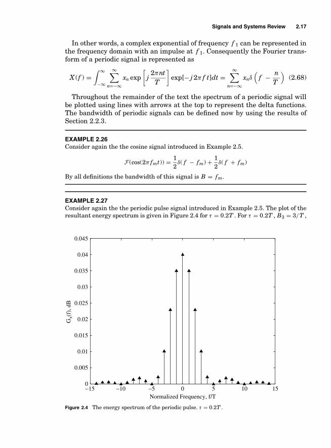
Signals and Systems Review 2.17
In other words, a complex exponential of frequency f 1 can be represented inthe frequency domain with an impulse at f 1. Consequently the Fourier trans-form of a periodic signal is represented as
X (f ) =∫ ∞
−∞
∞∑n=−∞
xn exp[
j2πnt
T
]exp[− j 2π f t]dt =
∞∑n=−∞
xnδ(
f − nT
)(2.68)
Throughout the remainder of the text the spectrum of a periodic signal willbe plotted using lines with arrows at the top to represent the delta functions.The bandwidth of periodic signals can be defined now by using the results ofSection 2.2.3.
EXAMPLE 2.26Consider again the the cosine signal introduced in Example 2.5.
F(cos(2π fmt)) = 12
δ( f − fm) + 12
δ( f + fm)
By all definitions the bandwidth of this signal is B = fm.
EXAMPLE 2.27Consider again the the periodic pulse signal introduced in Example 2.5. The plot of theresultant energy spectrum is given in Figure 2.4 for τ = 0.2T . For τ = 0.2T , B3 = 3/T ,
−15 −10 −5 0 5 10 150
0.005
0.01
0.015
0.02
0.025
0.03
0.035
0.04
0.045
Normalized Frequency, f/T
Gx(
f), d
B
Figure 2.4 The energy spectrum of the periodic pulse. τ = 0.2T .

2.18 Chapter Two
B40 = 152/T , and B98 = 26/T . Note the computation of B98 required a Matlab programto be written to sum the magnitude square of the Fourier series coefficients. B40 canonly be identified by expanding the x-axis in Figure 2.4 as the spectrum has not yet gone40 dB down in this figure.
2.2.5 Laplace Transforms
This text will use the one-sided Laplace transform for the analysis of tran-sient signals in communications systems. The one–sided Laplace transform ofa signal x(t) is
X (s) = L{x(t)} =∫ ∞
0x(t) exp[−st]dt (2.69)
The use of the one-sided Laplace transform implies that the signal is zero fornegative time. The inverse Laplace transform is given as
x(t) = 12π j
∮X (s) exp[st]ds (2.70)
The evaluation of the general inverse Laplace transform requires the evalu-ation of contour integrals in the complex plane. For most transforms of interestthe results are available in tables.
EXAMPLE 2.28
x(t) = sin(2π fmt) X (s) = 2π fm
s2 + (2π fm)2
x(t) = cos(2π fmt) X (s) = ss2 + (2π fm)2
2.3 Linear Time-Invariant Systems
Electronic systems are often characterized by the input/output relations. A blockdiagram of an electronic system is given in Figure 2.5, where x(t) is the inputand y(t) is the output.
Definition 2.14 A linear system is one in which superposition holds, i.e.,
ax1(t) + bx2(t) → ay1(t) + by2(t) (2.71)
Electronic Systemx t( ) y t( )
Figure 2.5 A system blockdiagram.

Signals and Systems Review 2.19
Definition 2.15 A time-invariant system is one in which a time shift in the input onlychanges the output by a time shift, i.e.,
x(t − τ ) → y(t − τ ) (2.72)
A linear time-invariant (LTI) system is described completely by an impulseresponse, h(t). The output of the linear system is the convolution of the inputsignal with the impulse response, i.e.,
y(t) =∫ ∞
−∞x(λ)h(t − λ)dλ = x(t) ∗ h(t) (2.73)
The Fourier transform (Laplace transform) of the impulse response is denotedthe frequency response (transfer function), H (f ) = F{h(t)}(H (s) = L{h(t)}),and by the convolution theorem for energy signals we have
Y (f ) = H (f )X (f ) (Y (s) = H (s)X (s)) (2.74)
Likewise the linear system output energy spectrum has a simple form
Gy(f ) = H (f )H ∗(f )Gx(f ) = |H (f )|2Gx(f ) = Gh(f )Gx(f ) (2.75)
EXAMPLE 2.29If a linear time-invariant filter had an impulse response given in Example 2.2, i.e.,
h(t) = 2Wsin(2πWt)
2πWt= 2Wsinc(2Wt)
it would result in an ideal lowpass filter. A filter of this form has two problems for animplementation: (1) the filter is anticausal and (2) the filter has an infinite impulseresponse. The obvious solution to having an infinite duration impulse response is totruncate the filter impulse response to a finite time duration. The way to make ananticausal filter causal is simply to time shift the filter response. Figure 2.6 (a) showsthe resulting impulse response when the ideal lowpass filter had a bandwidth of W =2.5 kHz and the truncation of the impulse response is 93 ms and the time shift of46.5 ms. The truncation will change the filter transfer function slightly while the delaywill only add a phase shift. The resulting magnitude for the filter transfer functionis shown in Figure 2.6 (b). If the voice signal of Example 2.3 is passed through this filter,then due to Eq. (2.75), the output energy spectrum should be filtered heavily outside of2.5 kHz and roughly the same within 2.5 kHz, as shown in Figure 2.7. Figure 2.7 showsthe measured energy spectrum of the input and output and these measured values matchexactly that predicted by theory. This is an example of how communications engineersmight use linear system theory to predict system performance. This signal will be usedas a message signal throughout the remainder of this text to illustrate the ideas ofanalog communication.

2.20 Chapter Two
0.038 0.042 0.046 0.05 0.054−2000
−1000
0
1000
2000
3000
4000
5000
Time, t, sec(a) The impulse response.
h(t)
−5000 −3000 −1000 0 1000 3000 5000−60
−50
−40
−30
−20
−10
0
10
Frequency, f, Hz(b) The spectrum, |H( f )|.
H(f
)
Figure 2.6 A lowpass filter impulse response and the spectrum. (a) The impulse response, h(t), of a filter obtainedby truncating (93 ms) and time-shifting (46.5 ms) (b) an ideal lowpass (W = 2.5 kHz) filter impulse response.
EXAMPLE 2.30In this example the signal from Example 2.1 is to be filtered by the filter from theprevious example. For this example we assume that Tp = 907µs. Figure 2.8 shows themeasured energy spectrum of the input and output, and Figure 2.9 shows the input andoutput time waveforms for this example. The impact of filtering in the frequency domainis clearly evident. The elimination of the high-frequency components of the pulse signaleliminates the sharp transitions and produces some ringing effects.
−5000 −3000 −1000 0 1000 3000 5000−80
−75
−70
−60
−55
−50
−45
−40
−35
−30
Frequency, f, Hz(a) Input
Gx(
f), d
B
−65
−5000 −3000 −1000 0 1000 3000 5000−80
−75
−70
−65
−60
−55
−50
−45
−40
−35
−30
Frequency, f, Hz(b) Output
Gy(
f)
Figure 2.7 (a) The energy spectrum of the voice signal before and (b) after filtering by a lowpass filter of bandwidth2.5 kHz.

Signals and Systems Review 2.21
−5000 −3000 −1000 0 1000 3000 5000−90−85
−80
−75
−70
−65
−60
−55
−50
−45
−40
Frequency, f, Hz
(a) Input
Gx(
f), d
B
−5000 −3000 −1000 0 1000 3000 5000−90−85
−80
−75
−70
−65
−60
−55
−50
−45
−40
Frequency, f, Hz
(b) Output
Gy(
f)Figure 2.8 (a) The energy spectrum of the pulse signal before and (b) after filtering by a lowpass filter of band-width 2.5 kHz.
For a periodic input signal the output of the LTI system will be a periodicsignal of the same period and have a Fourier series representation of
y(t) =∞∑
n=−∞H( n
T
)xn exp
[j 2πnt
T
]=
∞∑n=−∞
yn exp[
j 2πntT
](2.76)
where yn = H ( nT )xn. In other words the output of an LTI system with a periodic
input will also be periodic. The Fourier series coefficients are the product ofinput signal’s coefficients and the transfer function evaluated at the harmonicfrequencies.
0 0.002 0.004 0.006 0.008 0.01
0
0.2
0.4
0.6
0.8
1
Time, t, sec
(a) Input
x(t)
x(t)
0.042 0.044 0.046 0.048 0.0520.05
0
0.2
0.4
0.6
0.8
1
Time, t, sec
(b) Output
Figure 2.9 (a) The time domain signals of the pulse signal before and (b) after filtering by a lowpass filter ofbandwidth 2.5 kHz.

2.22 Chapter Two
EXAMPLE 2.31Consider the signal from Example 2.1, x(t) = cos(2π fmt) input into an arbitrary filtercharacterized with a transfer function H (f ). The output Fourier series coefficients are
fT = fm y1 = H ( fm)2
y−1 = H (− fm)2
xn = 0 (2.77)
and denoting the amplitude of the transfer funtion with HA(f ) and the phase of thetransfer function with HP (f ) the output signal is
y(t) = HA( fm) cos(2π fmt + HP ( fm)) (2.78)
EXAMPLE 2.32Consider the repeating pulse signal with 1/T = 500 Hz and τ = 2500 Hz from Example2.5, input into a filter with an impulse response given in Example 2.2, i.e.,
h(t) = 2Wsin(2πWt)
2πWt= 2Wsinc(2Wt)
where W = 2500 Hz. The input signal spectrum is given in Figure 2.4. The outputFourier series coefficients are the same over the passband of the filter and are zero out-side the passband. The output spectrum and output time plot are shown in Figure 2.10.
An important linear system for the study of frequency modulated (FM) signalsis the differentiator. The differentiator is described with the following transferfunction
y(t) = d nx(t)dtn ⇔ Y (f ) = ( j 2π f )nX (f ) (2.79)
−8000 −6000 −2000 0 2000 6000 80000
0.005
0.01
0.015
0.02
0.025
0.03
0.035
0.04
0.045
Frequency, f, Hz
Gy(
f), d
B
0 0.5 1 1.5 2 2.5 3 3.5 4× 10⁻³
−0.2
0
0.2
0.4
0.6
0.8
1
1.2
Time, t, sec
(b) Time signal(a) Spectrum
y(t)
Figure 2.10 A filtered repetitive pulse, τ = 1/2500 and T = 1/500.

Signals and Systems Review 2.23
2.4 Utilizing Matlab
The signals that are discussed in a course on communications are typicallydefined over a continuous time variable, e.g., x(t). Matlab is an excellent packagefor visualization and learning in communications engineering and will be usedliberally throughout this text. Unfortunately Matlab uses signals that are de-fined over a discrete time variable, x(k). Discrete time signal processing basicsare covered in the prerequisite signals and linear systems and comprehensivetreatments are given in [Mit98, OS99, PM88, Por97]. This section provides abrief discussion of how to transition between the continuous time functions(communication theory) and the discrete time functions (Matlab). The exam-ples considered in Matlab will reflect the types of signals you might measurewhen testing signals in the lab.
2.4.1 Sampling
The simplest way to convert a continuous time signal, x(t), into a discrete timesignal, x(k), is to sample the continuous time signal, i.e.,
x(k) = x(kTs + ε)
where Ts is the time between samples. The sample rate is denoted f s = 1Ts
. Thisconversion is an important part of analog–to–digital conversion (ADC) and isa common operation in practical communication system implementations. Thediscrete time version of the signal is a faithful representation of the continuoustime signal if the sampling rate is high enough.
To see that this is true it is useful to introduce some definitions for discretetime signals.
Definition 2.16 For a discrete time signal x(k), the discrete time Fourier transform(DTFT) is
X (e j 2π f ) =∞∑
k=−∞x(k)e j 2π f k (2.80)
For clarity when the frequency domain representation of a continuous timesignal is discussed it will be denoted as a function of f , e.g., X (f ) and whenthe frequency domain representation of a discrete time signal is discussed itwill be denoted as a function of e j 2π f , e.g., X (e j 2π f ). This DTFT is a continuousfunction of frequency and since no time index is associated with x(k), the rangeof where the function can potentially take unique values is f ∈ [−0.5, 0.5].Matlab has built-in functions to compute the discrete Fourier transform (DFT),which is simply the DTFT evaluated at uniformly spaced points.
For a sampled signal, the DTFT is related to the Fourier transform of thecontinuous time signal via [Mit98, OS99, PM88, Por97].
X (e j 2π f ) = 1Ts
∞∑n=−∞
X(
f − nTs
)(2.81)

2.24 Chapter Two
Examining Eq. (2.81) shows that if the sampling rate is higher than twicethe highest significant frequency component of the continuous time signal then
X (e j 2π f ) = 1Ts
X(
fTs
)(2.82)
and
X (f ) = Ts X (e j 2π( f Ts)) (2.83)
Note the highest significant frequency component is often quantified throughthe definition of the bandwidth (see Section 2.2.3). Consequently the rule ofthumb for sampling is that the sampling rate should be at least twice the band-width of the signal. A sampling rate of exactly twice the bandwidth of the signalis known as Nyquist’s sampling rate.
2.4.2 Integration
Many characteristics of continuous time signals are defined by an integral. Forexample, the energy of a signal is given in Eq. (2.1) as an integral. The Fouriertransform, the correlation function, convolution, and the power are other exam-ples of signal characteristics defined through integrals. Matlab does not havethe ability to evaluate integrals but the values of the integral can be approx-imated to any level of accuracy desired. The simplest method of computingan approximation solution to an integral is given by the Riemann sum firstintroduced in calculus.
Definition 2.17 A Riemann sum approximation to an integral is
∫ b
ax(t)dt ≈ b − a
N
N∑k=1
x
(a − ε + k(b − a)
N
)= h
N∑k=1
x(k) (2.84)
where ε ∈ [−(b − a)/N , 0] and h = b−aN is the step size for the sum.
A Riemann sum will converge to the true value of the finite integral as thenumber of points in the sum goes to infinity. Note that the DTFT for sampledsignals can actually be viewed as a Riemann sum approximation to the Fouriertransform.
2.4.3 Commonly Used Functions
This section details some Matlab functions that can be used to implement thesignals and systems that are discussed in this chapter. Help with the details ofthese functions is available in Matlab.
Standard Stuff■ cos — cosine function■ sin — sine function■ sinc — sinc function

Signals and Systems Review 2.25
■ sqrt — square root function■ log10 — log base ten, this is useful for working in dB■ max — maximum of a vector■ sum — sum of the elements of a vector
Complex signals■ abs — | • |■ angle — arg(•)■ real — [•]■ imag — �[•]■ conj — (•)∗
Input and Output■ plot — 2D plotting■ xlabel, ylabel, axis — formatting plots■ sound,soundsc — play vector as audio■ load — load data■ save — save data
Frequency Domain and Linear Systems■ fft — computes a discrete Fourier transform (DTF)■ fftshift — shifts an DFT output so when it is plotted it looks more like a
Fourier transform■ conv — convolves two vectors
2.5 Homework Problems
Problem 2.1. Let two complex numbers be given as
z1 = x1 + j y1 = a1 exp( j θ1) z2 = x2 + j y2 = a2 exp( j θ2) (2.85)
Find
(a) [z1 + z2]
(b) |z1 + z2|(c) �[z1z2]
(d) arg[z1z2]
(e) |z1z2|

2.26 Chapter Two
Problem 2.2. Plot, find the period, and find the Fourier series representation ofthe following periodic signals
(a) x(t) = 2 cos(200πt) + 5 sin(400πt)
(b) x(t) = 2 cos(200πt) + 5 sin(300πt)
(c) x(t) = 2 cos(150πt) + 5 sin(250πt)
Problem 2.3. Consider the two signals
x1(t) = m(t) cos(2π fct) x2(t) = m(t) sin(2π fct)
where the bandwidth of m(t) is much less than fc. Compute the simplest formfor the following four signals
(a) y1(t) = x1(t) cos(2π fct)
(b) y2(t) = x1(t) sin(2π fct)
(c) y3(t) = x2(t) cos(2π fct)
(d) y4(t) = x2(t) sin(2π fct)
Postulate how a communications engineer might use these results to recovera signal, m(t), from x1(t) or x2(t).
Problem 2.4. (Design Problem) This problem gives you a little feel for microwavesignal processing and the importance of the Fourier series. You have at yourdisposal
(1) a signal generator that produces ± 1 V amplitude square wave in a 1 � sys-tem where the fundamental frequency, f 1, is tunable from 1 kHz to 50 MHz
(2) an ideal bandpass filter with a center frequency of 175 MHz and a bandwidthof 30 MHz (±15 MHz).
The design problem is
(a) Select an f 1 such that when the signal generator is cascaded with the filterthat the output will be a single tone at 180 MHz. There might be more thanone correct answer (that often happens in real life engineering).
(b) Calculate the amplitude of the resulting sinusoid.
Problem 2.5. This problems exercises the signal and system tools. Compute theFourier transform of
(a)
x(t) ={
A 0 ≤ t ≤ Tp
0 elsewhere(2.86)

Signals and Systems Review 2.27
(b)
x(t) ={
Asin(
πtTp
)0 ≤ t ≤ Tp
0 elsewhere(2.87)
and give the value of A such that Eu = 1. Compute the 40-dB relative band-width, B40, of each signal.
Problem 2.6. This problem is an example of a problem which is best solved withthe help of a computer. The signal x(t) is passed through an ideal lowpass filterof bandwidth B/Tp Hz. For the signals given in Problem 2.5 with unit energymake a plot of the output energy versus B .
Hint: Recall the trapezoidal rule from calculus to approximately compute thisenergy.
Problem 2.7. This problem uses signal and system theory to compute the outputof a simple memoryless nonlinearity. An amplifier is an often used device in com-munication systems and is simply modeled as an ideal memoryless system, i.e.,
y(t) = a1x(t)
This model is an excellent model until the signal levels get large then non-linear things start to happen, which can produce unexpected changes in theoutput signals. These changes often have a significant impact in a communica-tion system design. As an example of this characteristic consider the system inFigure 2.11 with the following signal model
x(t) = b1 cos(200000πt) + b2 cos(202000πt)
the ideal bandpass filter has a bandwidth of 10 kHz centered at 100 kHz, andthe amplifier has the following memoryless model
y(t) = a1x(t) + a3x3(t)
Give the system output, z(t), as a function of a1, a3, b1, and b3.
Problem 2.8. (PD) A nonlinear device that is often used in communication systemsis a quadratic memoryless nonlinearity. For such a device if x(t) is the inputthe output is given as
y(t) = ax(t) + bx2(t)
x t( ) y t( ) z t( )Amplifier Ideal BPF
Figure 2.11 The system diagramfor Problem 2.7.

2.28 Chapter Two
(a) If x(t) = Acos(2π fmt), what is y(t) and Y (f )?
(b) If
X (f ) ={
A || f | − fc| ≤ fm
0 elsewhere(2.88)
what is y(t) and Y (f )?
(c) A quadratic nonlinearity is often used in a frequency doubler. What com-ponent would you need to add in series with this quadratic memorylessnonlinearity such that you could put a sine wave in and get a sine wave outof twice the input frequency?
Problem 2.9. Consider the following signal
x(t) = cos(2π f 1t) + a sin(2π f 1t)
= X A(a) cos(2π f 1t + X p(a)) (2.89)
(a) Find X A(a).
(b) Find X p(a).
(c) What is the power of x(t), Px?
(d) Is x(t) periodic? If so, what is the period and the Fourier seriesrepresentation of x(t)?
Problem 2.10. Consider a signal and a linear system as depicted in Figure 2.12where
x(t) = A+ cos(2π f 1t)
and
h(t) =
⎧⎪⎨⎪⎩
1√Tp
0 ≤ t ≤ Tp
0 elsewhere(2.90)
Compute the output y(t).
Problem 2.11. For the signal
x(t) = 23sin(2π147t)
2π147t(2.91)
x t( ) y t( )h t( ) Figure 2.12 The system forProblem 2.10.

Signals and Systems Review 2.29
(a) Compute X (f ).
(b) Compute Ex.
(c) Compute y(t) = d x(t)dt .
(d) Compute Y (f ).
Hint: Some of the computations have an easy way and a hard way so thinkbefore turning the crank!
Problem 2.12. The three signals seen in Figure 2.13 are going to be used to exer-cise your signals and systems theory. If no functional form is given for the pulse,assume ideal rectangular transitions to simplify the computations. Compute foreach signal
0
0.2
0.4
0.6
0.8
1
0 0.2 0.4 0.6 0.8 1
−1
−0.5
0
0.5
1
0 0.25 0.5Normalized Time, t/Tp
0.75 1
u 1(t
)
−1
−0.5
0
0.5
1
0 0.25 0.5Normalized Time, t/Tp
Normalized Time, t/Tp
0.75 1
u 2(t
)u 3
(t)
u t tTp
3 2( ) = sin
Figure 2.13 Pulse shapes considered for Problem 2.12.

2.30 Chapter Two
(a) The Fourier transform, Ui(f ), i = 1, 2, 3.
(b) The energy spectral density, Gui (f ).
(c) The correlation function, Vui (τ ). What is the energy, Eui ?
Hint: Some of the computations have an easy way and a hard way so thinkbefore turning the crank!
Problem 2.13. This problem looks at several simplifying approximations for com-plex numbers that will be useful in analyzing the characteristics of analogmodulations and demodulators. Assume z is a complex number of the form
z = 1 + ε1 + j ε2 (2.92)
where εi is a real number with εi � 1 for i = 1, 2.
(a) Show a logical argument to justify the approximation |z| ≈ 1 + ε1.
(b) Assume ε1 = ε2 and find the values of ε1, where this approximation resultsin a error of less than 1%.
(c) Show a logical argument to justify the approximation arg{z} ≈ ε2.
(d) Assume ε1 = ε2 and find the values of ε1, where this approximation resultsin a error of less than 1%.
Problem 2.14. Pulse shapes will be important in digital communication systems.A Gaussian pulse shape arises in several applications and is given as
x(t) = 1√2πσ 2
exp[− t2
2σ 2
](2.93)
(a) Plot x(t) for σ = 0.25, 1, 4.
(b) Calculate X (f ). Hint:
1√2π
∫ ∞
−∞exp[−x2
2+ ax]
d x = exp[
a2
2
](2.94)
(c) Plot GX (f ) for σ = 0.25, 1, 4 using a dB scale on the y-axis.
Problem 2.15. A common signal has a Fourier series representation of
x(t) = 4π
∞∑k=0
(−1)k
2k + 1cos(10π(2k + 1)t) (2.95)

Signals and Systems Review 2.31
G fx( )
−200 200 f
0.01
Figure 2.14 An example energy spectrum.
(a) Plot x(t) for one period of the signal.
(b) Find Px.
(c) What is the 98% power bandwidth, B98, of x(t)?
Problem 2.16. Show that
F−1{X ∗(f )} = x∗(−t) (2.96)
Problem 2.17. For the energy spectrum shown in Figure 2.14 find
(a) Ex.
(b) The 3dB bandwidth, B3.
(c) The 40dB bandwidth, B40.
(d) The 98% energy bandwidth, B98.
Problem 2.18. A signal has a series expansion given as
m(t) = 8π2
∞∑n=1
1(2n − 1)2 cos
(2π(2n − 1)t
T
)(2.97)
(a) Characterize the Fourier series.
(b) Find the 3-dB bandwidth, B3.
(c) Find the 40-dB bandwidth, B40.
(d) Find the 98% power bandwidth, B98.
(e) Find the 99% power bandwidth, B99.
Problem 2.19. Prove that B90 < B98.

2.32 Chapter Two
Problem 2.20. An energy spectrum has a peak value of 0.02. Find the value theenergy spectrum must go below to be
(a) 40-dB below the peak.
(b) 3-dB below the peak.
Problem 2.21. A concept that sometimes finds utility in engineering practice isthe concept of RMS bandwidth. The RMS bandwidth is defined as
WR =√∫ ∞
−∞f 2Gx(f )df (2.98)
For the energy spectrum in Figure 2.14 find the RMS bandwidth.
Problem 2.22. A concept that often finds utility in engineering practice is theconcept of group delay. For a linear system with a transfer function denoted
H (f ) = HA(f ) exp[ j Hp(f )] (2.99)
the group delay of this linear system is defined as
τg(f ) = − 12π
ddf
Hp(f ) (2.100)
Group delay is often viewed as the delay experienced by a signal at frequencyf when passing through the linear system H (f ).
(a) An ideal delay element has an impulse response given as h(t) = δ(t − τd ),where τd > 0 is the amount of delay. Find the group delay of an ideal delayelement.
(b) An example low pass filter has
H (f ) = 1j 2π f + a
(2.101)
Plot the group delay of this filter for 0 ≤ f ≤ 5a.
(c) Give a nontrivial H (f ) that has τg(f ) = 0. In your example is the filtercausal or anticausal?
Problem 2.23. (RW) An interesting characteristic of the Fourier transform is lin-earity and linearity can be used to compute the Fourier transform of complicatedfunctions by decomposing these function into sums of simple functions.
(a) Prove if y(t) = x1(t) + x2(t), then Y (f ) = X1(f ) + X2(f ).
(b) Find the Fourier transform of the signal given in Figure 2.15.

Signals and Systems Review 2.33
0.5 1.0−0.5−1.0
0.5
y t( )
t
1.5
1.0
Figure 2.15 The rocket signal.
2.6 Example Solutions
Problem 2.24. Recall that the Fourier series is given as
x(t) =∞∑
n=−∞xn exp
[j 2π
nT
t]
Each of these waveforms in this chapter can be put in a Fourier Series rep-resentation by the use of Euler’s formula or
cos(θ ) = 12
[e j θ + e− j θ ] (2.102)
sin(θ ) = 12 j
[e j θ − e− j θ ] (2.103)
(a)
x(t) = 2 cos(200πt) + 5 sin(400πt)
= exp[ j 2π(100)t] + exp[ j 2π(−100)t] + 5j 2 exp[ j 2π(200)t]
− 5j 2 exp[ j 2π(−200)t]
The waveform is plotted in Figure 2.16.
1T = 100 x1 = 1 x−1 = 1
T = 0.01 x2 = 5j 2 x−2 = −5
j 2
xn = 0 otherwise

2.34 Chapter Two
0 0.01 0.02 0.03 0.04 0.05 0.06 0.07 0.08−10
−5
0
5
10
x(t)
0 0.01 0.02 0.03 0.04 0.05 0.06 0.07 0.08−10
−5
0
5
10
x(t)
0 0.01 0.02 0.03 0.04 0.05 0.06 0.07 0.08−10
−5
0
5
10
x(t)
Time, t, sec
Figure 2.16 Plots of the time waveforms for Problem 2.2.
(b) x(t) = 2 cos(200πt) + 5 sin(300πt). The waveform is plotted in Figure 2.16.
1T = 50 x2 = 1 x−2 = 1
T = 0.02 x3 = 5j 2 x−3 = −5
j 2
xn = 0 otherwise
(c) x(t) = 2 cos(150πt) + 5 sin(250πt). The waveform is plotted in Figure 2.16.
1T = 25 x3 = 1 x−3 = 1
T = 0.04 x5 = 5j 2 x−5 = −5
j 2
xn = 0 otherwise
Problem 2.25. The output of the quadratic nonlinearity is modeled as
y(t) = ax(t) + bx2(t) (2.104)

Signals and Systems Review 2.35
It is useful to recall that multiplication in the time domain results in convo-lution in the frequency domain, i.e.,
z(t) = x(t) × x(t) Z(f ) = X (f ) ∗ X (f ) (2.105)
(a) x(t) = Acos(2π fmt), which results in
y(t) = aAcos(2π fmt) + bA2 cos2(2π fmt)
= aAcos(2π fmt) + bA2(
12
+ 12
cos(4π fmt))
= aA2
exp[ j 2π fmt] + aA2
exp[− j 2π fmt] + bA2
2
+bA2
4exp[ j 4π fmt] + bA2
4exp[− j 4π fmt] (2.106)
The frequency domain representation for the output signal is given as
Y (f ) = aA2
δ( f − fm) + aA2
δ( f + fm) + bA2
2δ(f ) + bA2
4δ( f − 2 fm)
+ bA2
4δ( f + 2 fm) (2.107)
The first two terms in Eq. (2.107) are due to the linear term in Eq. (2.104)while the last three terms are due to the square law term. It is interestingto note that these last three terms can be viewed as being obtained byconvolving the two “delta” function frequency domain representation of acosine wave, i.e., 2 cos(2π fmt) = exp[ j 2π fmt] + exp[− j 2π fmt], with itself.
(b) The input signal is
X (f ) ={
A || f | − fc| ≤ fm
0 elsewhere(2.108)
Taking the inverse Fourier transform gives
x(t) = 4Afmsin(π fmt)
π fmtcos(2π fct) (2.109)
The output time signal of this quadratic nonlinearity is
y(t) = 4aAfmsin(π fmt)
π fmtcos(2π fct) + b
(4Afm
sin(π fmt)π fmt
cos(2π fct))2
= 4aAfmsin(π fmt)
π fmtcos(2π fct) + b
(4Afm
sin(π fmt)π fmt
)2
×(
12
+ 12
cos(4π fct))
(2.110)

2.36 Chapter Two
f
Y f( )
4
2AfmbAa
fc2 fm−2 fm 2 2−fc fc fmfm+ 2 fc
Afmb
Figure 2.17 Output spectrum of the quadratic nonlinearity for part (b).
The frequency domain representation of y(t) can be computed by taking theFourier transform or by using Y (f ) = aX (f )+b(X (f )∗ X (f )). The resultingFourier transform is plotted in Figure 2.17.
(c) Looking at part (a) one can see that a tone in will produce a tone out if allfrequencies except those at 2 fm are eliminated. Consequently a quadraticnonlinearity followed by a BPF will produce a frequency doubler. The blockdiagram for this frequency doubler is shown in Figure 2.18.
2.7 Miniprojects
Goal: To give exposure
1. To a small scope engineering design problem in communications
2. To the dynamics of working with a team
3. To the importance of engineering communication skills (in this case oralpresentations)
Presentation: The forum will be similar to a design review at a company(only much shorter). The presentation will be of 5 minutes in length with anoverview of the given problem and solution. The presentation will be followedby questions from the audience (your classmates and the professor). Each teammember should be prepared to make the presentation on the due date.
cos(2π fct) C cos(4π fct)QuadraticNonlinearity
BPF@2fc
Figure 2.18 A frequency doubler.

Signals and Systems Review 2.37
2.7.1 Project 1
Project Goals: In designing a communication system, bandwidth efficiencyis often a top priority. In analog communications one way to get bandwidthefficiency is to limit the bandwidth of the message signal. The big engineeringtrade-off is how narrow to make the bandwidth of the message signal. If thebandwidth is made too narrow, the message will be distorted. If the bandwidthis made too wide, spectrum will be wasted. This project examines this trade-offfor a realistic signal.
Get the Matlab file sigsex2.m from the class web page along with the com-puter generated voice signal. Use this file to make an estimate how small thebandwidth of a voice signal can be and still enable high-fidelity communications.There is no single or right answer to the problem but engineering judgmentmust be used. How would your answer be different if you were only concernedwith word recognition or if you wanted to maintain speaker recognition as well.Please detail your reasons for your solution. Relate your results to the differentnotions of bandwidth that were discussed in the text.
2.7.2 Project 2
Project Goals: The computation of a percent energy bandwith, BP , requiresa numerical integration to be performed for most signals that are used in com-munications. This project will assign you to do this integration for a realisticsignal.
Get the computer-generated voice signal from the class web page. Write aprogram to estimate the the 90% bandwidth of this signal.

This page intentionally left blank

Chapter
3Review of Probability and
Random Variables
This chapter is intended to review introductory material on random variables,typically covered in an undergraduate curriculum. The most important use ofthis chapter will be the introduction of the notation used in this text. More proofswill be provided in this chapter than the last chapter because typically thissubject matter is not as synthesized at the start of a senior level communicationscourse. Texts that give a more detailed treatment of the subject of probabilityand random variables are [DR87, LG89, Hel91, CM86, Dev00, Sti99, YG98].
3.1 Axiomatic Definitions of Probability
Characterization of random events or experiments is critical for communicationsystem design and analysis. A majority of the analyses of random events orexperiments are extensions of the simple axioms or definitions presented in thissection. A random experiment is characterized by a probability space consistingof a sample space �, a field F , and a probability measure P (•). This probabilityspace will be denoted (�, F , P ).
EXAMPLE 3.1Consider the random experiment of rolling a fair dice
� = {1, 2, 3, 4, 5, 6} (3.1)
The field, F , is the set of all possible combinations of outputs, i.e., consider the fol-lowing outcomes A1 = {the die shows a 1}, A2 = {the die shows an even number}, A3 ={the die shows a number less than 4}, and A4 = {the die shows an odd number}, whichimplies
A1, A2, A3, A4 ∈ F (3.2)
3.1
Copyright © 2007 by The McGraw-Hill Companies. Click here for terms of use.

3.2 Chapter Three
Definition 3.1 Events A and B are mutually exclusive if A∩ B = ∅Axioms of Probability. A probability measure, P , for a probability space(�, F , P ) with events A, B ∈ F must satisfy the following axioms
■ For any event A, P (A) ≥ 0■ P (�) = 1■ If A and B are mutually exclusive events then P ( A∪ B ) = P ( A) + P (B ).
These three axioms are the building blocks for probability theory and anunderstanding of random events that characterize communication systemperformance.
EXAMPLE 3.2Example 3.1(cont.). The rolling of a fair die
A1 = {1} A2 = {2, 4, 6} A3 = {1, 2, 3} A4 = {1, 3, 5}
P [{1}] = P [{2}] = · · · = P [{6}] (3.3)
P [A1] = 16
P [A2] = 12
P [A3] = 12
P [A4] = 12
Definition 3.2 (Complement) The complement of a set A, denoted AC , is the set of allelements of � that are not elements of A.
Theorem 3.1 Poincare For N events A1, A2, .....AN
P [A1 ∪ A2 ∪ .... ∪ AN ] = S1 − S2 + · · · · +(−1)N −1SN
where
Sk =∑
i1<i2<....<ik
P [Ai1 ∩ Ai2 ∩ .... ∩ Aik ] i1 ≥ 1, ik ≤ N
Proof: The results are given for N = 2 and the proof for other cases is similar(if not more tedious). Note that events A and B ∩ AC are mutually exclusiveevents. Consequently we have
P [A∪ B ] = P [(A∩ BC ) ∪ B ] = P [A∩ BC ] + P [B ] (3.4)
P [A∪ B ] = P [(B ∩ AC ) ∪ A] = P [B ∩ AC ] + P [A] (3.5)
P [A∪ B ] = P [(A∩ BC ) ∪ ( A∩ B ) ∪ (B ∩ AC )]
= P [A∩ BC ] + P [A∩ B ] + P [B ∩ AC ] (3.6)
Using Eq. (3.4) + Eq. (3.5) − Eq. (3.6) gives the desired result. �

Review of Probability and Random Variables 3.3
EXAMPLE 3.3
P [A∪ B ] = P [A] + P [B ] − P [A∩ B ]
P [A∪ B ∪ C] = P [A] + P [B ] + P [C] − P [A∩ B ]
− P [B ∩ C] − P [A∩ C] + P [A∩ B ∩ C] (3.7)
EXAMPLE 3.4Example 3.1(cont.).
P [A2 ∪ A3] = P [A2] + P [A3] − P [A2 ∩ A3] (3.8)
A2 ∩ A3 = 2 P [A2 ∩ A3] = 16
(3.9)
P [A2 ∪ A3] = P [1, 2, 3, 4, 6] = 12
+ 12
− 16
= 56
(3.10)
Definition 3.3 (Conditional Probability) Let (�, F , P ) be a probability space with setsA, B ∈ F and P [B ] �= 0. The conditional or a posteriori probability of event A given anevent B , denoted P [A|B ], is defined as
P [A|B ] = P [A∩ B ]P [B ]
P [A|B ] is interpreted as event A’s probability after the experiment has beenperformed and event B is observed.
Definition 3.4 (Independence) Two events A, B ∈ F are independent if and only if
P [A∩ B ] = P [A]P [B ]
Independence is equivalent to
P [A|B ] = P [A] (3.11)
For independent events A and B , the a posteriori or conditional probabilityP [A|B ] is equal to the a prioir probability P [A]. Consequently, if A and B areindependent, then observing B reveals nothing about the relative probabilityof the occurrence of event A.

3.4 Chapter Three
EXAMPLE 3.5Example 3.1(cont.). If the die is rolled and you are told the outcome is even, A2, howdoes that change the probability of event A3?
P [A3|A2] = P (A2 ∩ A3)P (A2)
=1612
= 13
Since P [A3|A2] �= P [A3], event A3 is not independent of event A2.
Definition 3.5 A collectively exhaustive set of events is one for which
A1 ∪ A2 ∪ . . . . ∪ AN = �
Theorem 3.2 Total Probability For N mutually exclusive, collectively exhaustiveevents ( A1, A2, . . . . . AN ) and B ∈ �, then
P [B ] =N∑
i=1
P [B |Ai]P [Ai]
Proof: The probability of event B can be written as
P [B ] = P [B ∩ �] = P
[B ∩
N⋃i=1
Ai
]= P
[N⋃
i=1
B ∩ Ai
]
The events B ∩ Ai are mutually exclusive, so
P [B ] = P
[N⋃
i=1
B ∩ Ai
]=
N∑i=1
P [B ∩ Ai] =N∑
i=1
P [B |Ai]P [Ai] �
EXAMPLE 3.6Example 3.1(cont.). Note A2 and A4 are a set of mutually exclusive collectively exhaust-ive events with
P [A3|A4] = P [A3 ∩ A4]P [A4]
= P [{1, 3}]P [A4]
=2612
= 23
This produces
P [A3] = P [A3|A2]P ( A2) + P [A3|A4]P (A4) = 13
[12
]+[
23
][12
]= 3
6= 1
2
Theorem 3.3 (Bayes) For N mutually exclusive, collectively exhaustive events{A1, A2, . . . AN } and B ∈ �, then the conditional probability of the event Aj given that

Review of Probability and Random Variables 3.5
event B is observed is
P [Aj |B ] = P [B |Aj ]P [Aj ]P [B ]
= P [B |Aj ]P [Aj ]∑Ni=1 P [B ∩ Ai]
Proof: The definition of conditional probability gives
P [Aj ∩ B ] = P [Aj |B ]P [B ] = P [B |Aj ]P [Aj ]
Rearrangement and total probability complete the proof. �
EXAMPLE 3.7(Binary symmetric channel) A facsimile machine divides a document up into smallregions (i.e., pixels) and decides whether each pixel is black or white. Reasonable apriori statistics for facsimile transmission is
P [A pixel is white] = P [W ] = 0.8 P [A pixel is black] = P [B ] = 0.2
This pixel value is transmitted across a telephone line and the receiving fax machinemakes a decision about whether a black or white pixel was sent. Figure 3.1 is a sim-plified representation of this operation in an extremely noisy situation. If a black pixelis decoded (B D) what is the probability a white pixel was sent, P (W |B D)? Bayes rulegives a straightforward solution to this problem, i.e.,
P (W |B D) = P [B D|W ]P [W ]P [B D]
(3.12)
= P [B D|W ]P [W ]P [B D|W ]P [W ] + P [B D|B ]P [B ]
= (0.1)0.8(0.1)(0.8) + (0.9)(0.2)
= 0.3077 (3.13)
WhitePixelSent
BlackPixelSent
WhitePixelDecoded
BlackPixelDecodedP BD B[ ] = 0 9.
P BDW[ ] = 0 1.
P WDW[ ] = 0 9.
P WD B[ ] = 0 1.
Figure 3.1 The binary symmetric channel.

3.6 Chapter Three
3.2 Random Variables
In communications, the information transmission is often corrupted by randomnoise. This random noise manifests itself as a random voltage (a real number)at the output of the electrical circuits in the receiver. The concept of a randomvariable (RV) links the axiomatic definition of probability with these observedreal random numbers. A random variable has an underlying random exper-iment. The set of all experimental outcomes are denoted � and a particularoutcome of the random experiment is denoted with ω.
Definition 3.6 Let (�, F , P ) be a probability space. A real random variable X (ω) is asingle-valued function or mapping from � to the real line (R).
There are three types of random variables: discrete, continuous, and mixed.A discrete random variable has a finite (or countably infinite) number of possiblevalues. A continuous random variable takes values in some interval of the realline of nonzero length. A mixed random variable is a convex combination of adiscrete and a continuous random variable. To simplify the notation when noambiguity exists, X represents the random variable X (ω) (the experimentaloutcome index is dropped) and x = X (ω) represents a particular realization ofthis random variable.
Definition 3.7 An observed real number resulting from the random experiment isdenoted a sample from the random variable.
EXAMPLE 3.8Matlab has a built-in random number generator. In essence this function when executedperforms an experiment and produces a real number output (a sample of the randomvariable). Each time this function is run, a different real value is returned. Go to Matlaband type rand(1) and see what happens. Each time you run this function, it returns anumber that is unable to be predicted. The output can be characterized in many ways,but the outputs are not completely predictable.
Random variables are completely characterized by either of two related func-tions: the cumulative distribution function (CDF) or the probability densityfunction (PDF)1. These functions are the subject of the next two sections.
3.2.1 Cumulative Distribution Function
Definition 3.8 For a random variable X (ω), the CDF is a function FX (x) defined as
FX (x) = P ({ω : X (ω) ≤ x}) ∀ x ∈ R
1Continuous RVs have PDFs but discrete random variables have probability mass functions(PMF).

Review of Probability and Random Variables 3.7
•
0
•0
•0
•0
1 1
•0
•0
•0
1
(a) (b)
(c)
x x
x
Fx(x) Fx(x)
Fx(x)
Figure 3.2 Example CDF for (a) discrete RV, (b) continuous RV, and (c) mixed RV.
Again to simplify the notation when no ambiguity exists, the CDF of therandom variable X will be written as FX (x) = P (X ≤ x). Figure 3.2 showsexample plots of the CDF for discrete, continuous and mixed random variables.The discrete random variable has a CDF with a stairstep form, the steps occurat the points of the possible values of the random variable. The continuousrandom variable has a CDF, that is a continuous function and the mixed randomvariable has a CDF containing both intervals where the function is continuouswith non-zero derivative and points where the function makes a jumps.
Properties of a CDF■ FX (x) is a monotonically increasing function2, i.e.,
x1 < x2 ⇒ FX (x1) ≤ FX (x2)
■ 0 ≤ FX (x) ≤ 1■ FX (−∞) = P (X ≤ −∞) = 0 and FX (∞) = P (X ≤ ∞) = 1■ A CDF is right continuous, i.e., limh→0 FX (x + |h|) = FX (x)■ P (X > x) = 1 − FX (x) and P (x1 < X ≤ x2) = FX (x2) − FX (x1)■ The probability of the random variable taking a particular value, a, is given as
P (X = a) = FX (a) − limh→0
FX (x − |h|)
Continuous random variables take any value with zero probability since theCDF is continuous, while discrete and mixed random variables take values with
2This is sometimes termed a nondecreasing function.

3.8 Chapter Three
nonzero probabilities since the CDF has jumps. The discrete random variablehas a CDF with the form
FX (x) =N∑
k=1
P (X = ak)U (x − ak) (3.14)
where U () is the unit step function, N is the number of jumps in the CDF, andak are the locations of the jumps.
3.2.2 Probability Density Function
Definition 3.9 For a continuous random variable X (ω), the PDF is a function f X (x)defined as
f X (x) = d P (X (ω) ≤ x)dx
= dFX (x)dx
∀ x ∈ R (3.15)
Since the derivative in Eq. (3.15) can be rearranged to give
lim�→0
f X (x)� = lim�→0
P(
x − �
2< X (ω) ≤ x + �
2
),
the PDF can be thought of as the probability “density” in a very small intervalaround X = x. Discrete random variables do not have a probability “density”spread over an interval but do have probability mass concentrated at points. Sothe idea of a density function for a discrete random variable is not consistent.The analogous quantity to a PDF for a continuous RV in the case of a discreteRV is the probability mass function (PMF)
pX (x) = P (X = x)
The idea of the probability density function can be extended to discrete andmixed random variables by utilizing the notion of the Dirac delta function[CM86].
Properties of a PDF■ FX (x) = ∫ x
−∞ f X (β)dβ
■ f X (x) ≥ 0■ FX (∞) = 1 = ∫∞
−∞ f X (β)dβ
■ P (x1 < X ≤ x2) = ∫ x2
x1f X (β)dβ
Again, if there is no ambiguity in the expression, the PDF of the randomvariable X is written as f (x) and if there is no ambiguity about whether aRV is continuous or discrete, the PDF is written p(x). Knowing the PDF (orequivalently the CDF) allows you to completely describe any random eventassociated with a random variable.

Review of Probability and Random Variables 3.9
EXAMPLE 3.9The rand(•) function in Matlab produces a sample from what is commonly termed auniformly distributed random variable. The PDF for a uniformly distributed randomvariable is given as
f X (x) =
⎧⎨⎩
1b − a
a ≤ x ≤ b
0 elsewhere(3.16)
The function in Matlab has a = 0 and b = 1. Likewise the CDF is
FX (x) =
⎧⎪⎪⎨⎪⎪⎩
0 x ≤ ax − ab − a
a ≤ x ≤ b
1 x ≥ b
(3.17)
Experimenting in Matlab will give you some insight.
3.2.3 Moments and Statistical Averages
A communications engineer often calculates the statistical average of a functionof a random variable. The average value or expected value of a function g(X )with respect to a random variable X is
E(g(X )) =∫ ∞
−∞g(x) pX (x)dx
Average or expected values are numbers, that provide some partial informa-tion about the random variable. Average values are one number characteriza-tions of random variables but are not a complete description in themselves likea PDF or CDF. A good example of a statistical average often used to characterizeRVs is given by the mean value. The mean value is defined as
E(X ) = mX =∫ ∞
−∞xpX (x)dx
The mean is the average value of the random variable. The nth moment of arandom variable is a generalization of the mean and is defined as
E(X n) = mX ,n =∫ ∞
−∞xn pX (x)dx
The mean square value, E(X 2), is frequently used in the analysis of a commu-nication system (e.g., average power). Another function of interest is a centralmoment (a moment around the mean value) of a random variable. The nthcentral moment is defined as
E((X − mX )n) = σX ,n =∫ ∞
−∞(x − mX )n pX (x)dx

3.10 Chapter Three
The most commonly used second central moment is the variance, σX ,2, whichprovides a measure of the spread of a random variable around the mean. Thevariance has the shorthand notation σX ,2 = σ 2
X = var(X ). The relation betweenthe variance and the mean square value is given by
E(X 2) = m2X + σ 2
X
The expectation operator is linear, i.e.,
E(g1(x) + g2(x)) = E(g1(x)) + E(g2(x))
EXAMPLE 3.10Consider again the rand(•) function in Matlab as an example of a random variable.Since
f X (x) =
⎧⎨⎩
1b − a
a ≤ x ≤ b
0 elsewhere(3.18)
the mean is given as
E[X ] = 1b − a
∫ b
axdx = b2 − a2
2(b − a)= b + a
2(3.19)
and the variance is
var(X ) = (b − a)2
12(3.20)
3.2.4 The Gaussian Random Variable
The most common RV encountered in communications system analysis is theGaussian random variable. This RV is a very good approximation to manyof the physical phenomena that occur in electronic communications (e.g., thenoise voltage generated by thermal motion of electrons in conductors). Thereason for the common usage of the Gaussian RV is the Central Limit Theorem(see Section 3.3.5) and that analysis with Gaussian RVs is often tractable. Thissection will review the characteristics of the Gaussian RV. A Gaussian or normalRV, X , of mean mX and variance σ 2
X is denoted N (mX , σ 2X ). The Gaussian RV is a
continuous random variable taking values over the whole real line and a PDF of
f X (x) = 1√2πσ 2
X
exp[− (x − mX )2
2σ 2X
]
The Gaussian RV is characterized completely by its mean and variance. TheGaussian PDF is often referred to as the bell-shaped curve. The mean shifts thecentroid of the bell-shaped curve as shown in Figure 3.3(a). The variance is ameasure of the spread in the values the random variable realizes. A large vari-ance implies that the random variable is likely to take values far from the mean,

Review of Probability and Random Variables 3.11
−5 −4 −3 −2 −1 0 1 2 3
mean = 1
Variance = 0.25
Variance = 1
Variance = 4
mean = 0
4 50
0.05
0.1
0.15
0.2
0.25
0.3
0.35
0.4
x(a) Constant variance and varying mean.
σ2X = 1 and mX = 0, 1.
f X(x
)
−5 −4 −3 −2 −1 0 1 2 3 4 50
0.1
0.2
0.3
0.4
0.5
0.6
0.7
0.8
x(b) Constant mean and varying variance.
σ2X = 0.25, 1, 4 and mX = 0.
f X(X
)Figure 3.3 Plots of the PDF of a Gaussian random variable.
whereas a small variance implies that a large majority of the values a randomvariable takes is near the mean. As an example, Figure 3.3(b) plots the densityfunctions for three zero mean Gaussian RVs with variances of 0.25, 1, and 4.
A closed form expression for the CDF of the Gaussian RV does not exist. TheCDF is expressed as
FX (x) =∫ x
−∞
1√2πσ 2
X
exp[− (α − mX )2
2σ 2X
]dα
The CDF can be expressed in terms of the erf function [Ae72], which is given as
erf(z) = 2√π
∫ z
0e−t2
dt
The CDF of a Gaussian RV is then given as
FX (x) = 12
+ 12
erf(
x − mX√2σX
)
While the CDF of the Gaussian random variable is defined using differentfunctions by various authors, this function is used in this text because it iscommonly used in math software packages (e.g., Matlab). Three properties ofthe erf function important for finding probabilities associated with Gaussianrandom variables are given as
erf(∞) = 1
erfc(z) = 1 − erf(z)
erf(−z) = −erf(z)

3.12 Chapter Three
EXAMPLE 3.11The randn(•) function in Matlab produces a sample from a Gaussian distributed ran-dom variable with mX = 0 and σX = 1.
3.2.5 A Transformation of a Random Variable
In the analysis of communication system performance it is often necessary tocharacterize a random variable, which is a transformation of another randomvariable. This transformation is expressed as
Y = g(X )
This section is concerned with finding the PDF or the CDF of the randomvariable, Y . The general technique is a two step process.
Step 1: Find the CDF of Y as a sum of integrals over the random variable Xsuch that g(X ) < y. This is expressed mathematically as
FY (y) =∑
i
∫R i (y)
pX (β)dβ
where the R i(y) are intervals on the real line where X is such that g(X ) < y.
Step 2: Find the PDF by differentiating the CDF found in Step 1 using Leibnizrule from calculus.
pY (y) = dFY (y)dy
=∑
i
ddy
∫R i (y)
pX (β)dβ
Liebnitz Rule:
ddt
∫ b(t)
a(t)f (x, t)dx = f (b(t), t)
db(t)dt
− f (a(t), t)da(t)
dt+∫ b(t)
a(t)
∂ f (x, t)∂t
dx
To illustrate this technique, three examples are given, which are common tocommunication engineering.
EXAMPLE 3.12Y = aX (the output of a linear amplifier with gain a having an input random voltage X ).
Step 1:
FY (y) =
⎧⎪⎪⎨⎪⎪⎩∫ y
a−∞ pX (β)dβ i f a > 0
U (y) i f a = 0∫∞ya
pX (β)dβ i f a < 0

Review of Probability and Random Variables 3.13
where U (X ) is the unit step function. Note for a > 0 that only one interval of the realline exists, where g(x) ≤ y and that is x ∈ [−∞, y/a).
Step 2:
pY (y) =
⎧⎪⎨⎪⎩
1a pX ( y
a ) i f a > 0
δ(y) i f a = 0
− 1a pX ( y
a ) i f a < 0.
EXAMPLE 3.13Y = X 2 (the output of a square law or power detector with an input random voltage X ).
Step 1:
FY (y) =
⎧⎨⎩∫ √
y−√
y pX (β)dβ i f , y ≥ 0
0 i f y < 0
Step 2:
pY (y) =
⎧⎨⎩
12√
y pX (√
y) + 12√
y pX (−√y) i f y ≥ 0
0 i f y < 0
EXAMPLE 3.14Y = XU (X ). This example corresponds to the output of an ideal diode with an inputrandom voltage X .
Step 1:
FY (y) ={∫ y
−∞ pX (β)dβ i f y ≥ 0
0 i f y < 0
= U (y)∫ y
−∞pX (β)dβ
= U (y)FX (y) (3.21)
Step 2:
pY (y) = U (y) pX (y) + δ(y)FX (0)

3.14 Chapter Three
3.3 Multiple Random Variables
In communication engineering, performance is often determined by more thanone random variable. To analytically characterize the performance, a jointdescription of the random variables is necessary. All of the descriptions of asingle random variable (PDF, CDF, moments, etc.) can be extended to the setsof random variables. This section highlights these extensions.
3.3.1 Joint Density and Distribution Functions
Again the random variables are completely characterized by either the jointCDF or the joint PDF. Note, similar simplifications in notation will be usedwith joint CDFs and PDFs, as was introduced in Section 3.2, when no ambiguityexisted.
Definition 3.10 The joint CDF of two random variables is
FXY (x, y) = P ({X ≤ x} ∩ {Y ≤ y}) = P (X ≤ x, Y ≤ y)
Properties of the Joint CDF■ FXY (x, y) is a monotonically nondecreasing function, i.e.,
x1 < x2 and y1 < y2 ⇒ FXY (x1, y1) ≤ FXY (x2, y2)
■ 0 ≤ FXY (x, y) ≤ 1■ FXY (−∞, −∞) = P (X ≤ −∞, Y ≤ −∞) = 0 and FXY (∞, ∞) = P (X ≤
∞, Y ≤ ∞) = 1■ FXY (x, −∞) = 0 and FXY (−∞, y) = 0■ FX (x) = FXY (x, ∞) and FY (y) = FXY (∞, y)■ P (x1 < X ≤ x2, y1 < Y ≤ y2) = FXY (x2, y2) − FXY (x1, y2) − FXY (x2, y1) +
FXY (x1, y1)
Definition 3.11 For two continuous random variables X and Y , the joint PDF,f XY (x, y), is
f XY (x, y) = ∂2 P (X ≤ x, Y ≤ y)∂x∂y
= ∂2 FXY (x, y)∂x∂y
∀ x, y ∈ R
Note, jointly distributed discrete random variables have a joint PMF,pXY (x, y), and as the joint PMF and PDF have similar characteristics thistext often uses pXY (x, y) for both functions.
Properties of the Joint PDF or PMF■ FXY (x, y) = ∫ y
−∞∫ x
−∞ pXY (α, β)dαdβ
■ pXY (x, y) ≥ 0■ pX (x) = ∫∞
−∞ pXY (x, y)dy and pY (y) = ∫∞−∞ pXY (x, y)dx
■ P (x1 < X ≤ x2, y1 < Y ≤ y2) = ∫ x2
x1
∫ y2
y1pXY (α, β)dαdβ

Review of Probability and Random Variables 3.15
Definition 3.12 Let X and Y be random variables defined on the probability space(�, F , P ). The conditional or a posteriori PDF of Y given X = x, is
pY |X (y|X = x) = pXY (x, y)pX (x)
(3.22)
The conditional PDF, pY |X (y|X = x), is the PDF of the random variable Y afterthe random variable X is observed to take the value x.
Definition 3.13 Two random variables x and y are independent if and only if
pXY (x, y) = pX (x) pY (y)
Independence is equivalent to
pY |X (y|X = x) = pY (y)
i.e., Y is independent of X if no information is in the RV X about Y in the sensethat the conditional PDF is not different than the unconditional PDF.
EXAMPLE 3.15In Matlab each time rand(•) or randn(•) is executed it returns an ostensibly inde-pendent sample from the corresponding uniform or Gaussian distribution.
Theorem 3.4 Total Probability For two random variables X and Y the marginal densityof Y is given by
pY (y) =∫ ∞
−∞pY |X (y|X = x) pX (x)dx
Proof: The marginal density is given as (Property 3 of PDFs)
pY (y) =∫ ∞
−∞pXY (x, y)dx
Rearranging Eq. (3.22) and substituting completes the proof. �
Theorem 3.5 Bayes For two random variables X and Y the conditional density isgiven by
pY |X (y|X = x) = pX |Y (x|Y = y) pY (y)pX (x)
= pX |Y (x|Y = y) pY (y)∫∞−∞ pXY (x, y)dy
Proof: The definition of conditional probability gives
pXY (x, y) = pY |X (y|X = x) pX (x) = pY |X (x|Y = y) pY (y)
Rearrangement and total probability completes the proof. �

3.16 Chapter Three
A majority of the results presented in this section correspond to two randomvariables. The extension of these concepts to three or more random variablesis straightforward.
3.3.2 Joint Moments and Statistical Averages
Joint moments and statistical averages are also of interest in communicationsystem engineering. The general statistical average of a function g(X , Y ) of tworandom variables X and Y is given as
E[g(X , Y )] =∫ ∞
−∞
∫ ∞
−∞g(x, y) pXY (x, y)dxdy
A commonly used joint moment or statistical average is the correlation be-tween two random variables X and Y, defined as
E[XY ] = corr(X , Y ) =∫ ∞
−∞
∫ ∞
−∞xypXY (x, y)dxdy
A frequently used joint central moment is the covariance between two randomvariables x and y, defined as
E[(X − mX )(Y − mY )] = cov(X , Y ) =∫ ∞
−∞
∫ ∞
−∞(x − mX )(y − mY ) pXY (x, y)dxdy
Definition 3.14 The correlation coefficient is
ρXY = cov(X , Y )√var(X )var(Y )
= E[(X − mX )(Y − mY )]σX σY
The correlation coefficient is a measure of the statistical similarity of tworandom variables. If |ρXY | = 1 for random variables X and Y , then X is ascalar multiple of Y . If ρXY = 0 then the random variables are uncorrelated.Values of |ρXY | between these two extremes provide a measure of the similarityof the two random variables (larger |ρXY | being more similar).
3.3.3 Two Gaussian Random Variables
Two jointly Gaussian random variables, X and Y , have a joint densityfunction of
f XY (x, y) = 1
2πσX σY
√1 − ρ2
XY
× exp[− 1
2(1 − ρ2XY )
((x − mX )2
σ 2X
− 2ρXY (x − mX )(y − mY )σX σY
+ (y − mY )2
σ 2Y
)]
where mX = E(X ), mY = E(Y ), σ 2X = var(X ), σ 2
Y = var(Y ), and ρXY is thecorrelation coefficient between the two random variables X and Y . This densityfunction results in a three-dimensional bell-shaped curve which is stretched and

Review of Probability and Random Variables 3.17
−4−2
0
24
−4
−2
0
2
40
0.05
0.1
0.15
0.2
xy
f XY
(x, y
)
Figure 3.4 Plots of the joint PDF of two zero mean, unit variance, uncorrelatedGaussian random variables.
shaped by the means, variances, and the correlation coefficient. As an example,Figure 3.4 is a plot of the joint density function of two zero mean, unit variance,uncorrelated (ρXY = 0) Gaussian random variables. The uncorrelatedness of thetwo random variables is what gives this density function its circular symmetry.In fact, for Gaussian random variables uncorrelatedness implies that the tworandom variables are independent, i.e.,
f XY (x, y) = f X (x) f Y (y)
Changing the mean in the bivariate Gaussian density function again simplychanges the center of the bell-shaped curve. Figure 3.5(a) is a plot of a bivariateGaussian density function with mX = 1, mY = 1, σX = 1, σY = 1, and ρXY =0. The only difference between Figure 3.5(a) and Figure 3.4 (other than theperspective) is a translation of the bell shape to the new mean value (1,1).Changing the variances of joint Gaussian random variables changes the relativeshape of the joint density function much like that shown in Figure 3.3(b).
The effect of the correlation coefficient on the shape of the bivariate Gaus-sian density function is a more interesting concept. Recall that the correlationcoefficient is
ρXY = cov(X , Y )√var(X )var(Y )
= E[(X − mX )(Y − mY )]σX σY
If two random variables have a correlation coefficient greater than zero thenthese two random variables tend probabilistically to take values that are on the

3.18 Chapter Three
(a) Nonzero means. mX = 1, mY = 1, σX = 1,σY = 1, ρXY = 0.
−4−2
2−1
1−3
03 4
−4
−20
2
40
0.05
0.1
0.15
0.2
x
y
f XY
(x, y
)
(b) Nonzero correlation coefficient. mX = 0,mY = 0, σX = 1, σY = 1, ρXY = 0.9.
0.4
0.3
f XY
(x, y
)
0.2
0.1
04
2
0
−2
−3 −2 −1 0x
y1 2 3 4
−4 −4
Figure 3.5 Plots of the joint PDF of two unit variance Gaussian random variables.
same side of their mean value (if the random variables were zero mean then theywould tend to have the same sign). Also if these two random variables have acorrelation coefficient close to unity then they probabilistically behave in a verysimilar fashion. A good example of this characteristic is seen in Figure 3.5(b),which shows a plot of a bivariate Gaussian with mX = 0, mY = 0, σX = 1,σY = 1, and ρXY = 0.9.
While it is easy to see that the marginal densities, i.e.,
f X (x) =∫ ∞
−∞f XY (x, y)dy
from Figure 3.5(b) would be the same as the those obtained in Figure 3.4, theconditional densities would be much different, e.g.,
f X |Y (x|y) = 1
σX
√2π(1 − ρ2
XY
)× exp
[− 1
2σ 2X
(1 − ρ2
XY
) (x − mX − ρXY σX
σY(y − mY )
)2]
(3.23)
It should be noted that Eq. (3.23) says that for a pair of jointly Gaussianrandom variables, the distribution of one of the Gaussian random variablesconditioned on the other Gaussian random variable is also a Gaussian distri-bution with
E[X |Y = y] = mX + ρXY σX
σY(y − mY ) var(X |Y = y) = σ 2
X
(1 − ρ2
XY
)(3.24)
Since the random variables whose PDF is shown in Figure 3.5(b) are highlycorrelated, the resulting values the random variables take are very similar.

Review of Probability and Random Variables 3.19
This is reflected in the knife edge characteristic that the density function takesalong the line Y = X .
3.3.4 Transformations of Random Variables
In general, the problem of finding a probabilistic description (joint CDF orPDF) of a joint transformation of random variables is very difficult. To simplifythe presentation, two of the most common and practical transformations willbe considered: the single function of n random variables and the one-to-onetransformation.
Single Function of n Random Variables
A single function transformation of n random variables is expressed as
Y = g(X1, X2, . . . , Xn)
where X1, . . . , Xn are the n original random variables. This section is concernedwith finding the PDF or the CDF of the random variable Y . The general tech-nique is the identical two step process used for a single random variable (theregions of integration now become volumes instead of intervals).
Step 1: Find the CDF of Y as a sum of integrals over the random variablesX1 . . . Xn. This is expressed mathematically as
FY (y) =∑
i
∫· · ·R i(y)
∫pX1···Xn(x1, x2 · · · xn)dx1 · · · dxn
where the R i(y) are n dimensional volumes where X1 . . . Xn are such thatg(X1, . . . , Xn) < y.
Step 2: Find the PDF by differentiating the CDF found in Step 1 using Leibnizrule, i.e.,
pY (y) = dFY (y)dy
=∑
i
ddy
∫· · ·R i(y)
∫pX1···Xn(x1, x2, . . . , xn)dx1 · · · dxn
EXAMPLE 3.16A transformation which is very important for analyzing the performance of the standard
demodulator used with amplitude modulation (AM) is Y =√
X21 + X2
2.
Step 1:
FY (y) = P(√
X21 + X2
2 ≤ y)
= U (y)∫ y
−ydx1
∫ √y2−x21
−√
y2−x21
pX1 X2 (x1, x2)dx2

3.20 Chapter Three
Step 2:
pY (y) = U (y)∫ y
−y
y√y2 − x2
1
[pX1 X2
(x1,√
y2 − x21
)+ pX1 X2
(x1, −√
y2 − x21
)]dx1
If in this example X1 and X2 are independent (ρ = 0) and zero mean Gaussian randomvariables with equal variances, the joint density is given as
f X1 X2 (x1, x2) = 1
2πσ 2X
exp
(− x2
1 + x22
2σ 2X
)
and f Y (y) reduces to
f Y (y) = y
σ 2X
exp
(− y2
2σ 2X
)U (y) (3.25)
This PDF is known as the Rayleigh density and appears quite frequently in commu-nication system analysis.
One-to-One Transformations
Consider a one-to-one transformation of the form
Y1 = g1(X1, X2, · · · , Xn)
Y2 = g2(X1, X2, · · · , Xn)...
Yn = gn(X1, X2, · · · , Xn) (3.26)
Since the transformation is one-to-one, the inverse functions exist and aregiven as
X1 = h1(Y1, Y2, ..., Yn)
X2 = h2(Y1, Y2, ..., Yn)...
Xn = hn(Y1, Y2, ..., Yn) (3.27)
Since the probability mass in infinitesimal volumes in both the original X coor-dinate system and the Y coordinate system must be identical, the PDF of theY ’s is given as
pY (y1, y2, . . . yn) = |J |pX (h1(y1, y2, . . . yn), . . . , hn(y1, y2, . . . yn))

Review of Probability and Random Variables 3.21
where |J | is the Jacobian defined as
|J | =
∣∣∣∣∣∣∣∣∣∣∣∣
∂x1∂y1
∂x2∂y1
. . . ∂xn∂y1
∂x1∂y2
∂x2∂y2
. . . ∂xn∂y2
.... . .
∂x1∂yn
∂x2∂yn
. . . ∂xn∂yn
∣∣∣∣∣∣∣∣∣∣∣∣EXAMPLE 3.17A one-to-one transformation which is very important in communications is
Y1 =√
X21 + X2
2 X1 = Y1 sin(Y2)
Y2 = tan−1( X1
X2
)X2 = Y1 cos(Y2)
The Jacobian of the transformation is given by |J | = Y1 which results in the jointdensity of the transformed random variables being expressed as
pY1Y2 (y1, y2) = y1 pX1 X2 (y1 sin(y2), y1 cos(y2))
3.3.5 Central Limit Theorem
Theorem 3.6 If Xk is a sequence of independent, identically distributed (i.i.d.) randomvariables with mean mx and variance σ 2 and Yn is a random variable defined as
Yn = 1√nσ 2
n∑k=1
(Xk − mx)
then
limn→∞ pYn(y) = 1√
2πexp
[− y2
2
]= N (0, 1)
Proof: The proof uses the characteristic function, a power series expansion, andthe uniqueness property of the characteristic function. Details are available inmost introductory texts on probability [DR87, LG89, Hel91]. �
The central limit theorem (CLT) implies that the sum of arbitrarily dis-tributed random variables tends to a Gaussian random variable as the numberof terms in the sum gets large. Because many physical phenomena in communi-cations systems are due to interactions of large numbers of events (e.g., randomelectron motion in conductors or large numbers of scatters in wireless propa-gation), this theorem is one of the major reasons why the Gaussian randomvariable is so prevalent in communication system analysis.

3.22 Chapter Three
3.3.6 Multiple Dimensional Gaussian Random Variables
The most common situation encountered in communication system design andanalysis is for the corrupting noise samples to be Gaussian random variables.Analytically this is very fortunate since a simple closed-form expression for thejoint PDF of L Gaussian random variables is
f �N (�n) = 1√(2π )L det(CN )
exp[
− 12
(�n − �mN )T C−1N (�n − �mN )
](3.28)
where �N is an L × 1 vector defined as
�N = [N1, . . . , NL]T
�mN is the mean vector of �N , and CN is the L × L covariance matrix of thevector �N . The Gaussian assumption is rather powerful. It accurately modelsnoise in most communication systems and the joint PDF, which is a completeprobabilistic description of the random process, is given in terms of only thefirst and second moments.
Definition 3.15 A cross-covariance matrix between two real random vectors is
CXY = E[( �X − �mx)( �Y − �my)T ] (3.29)
Definition 3.16 If �X and �Y are both Gaussian random vectors then �X conditioned on�Y = �y is a Gaussian random vector with
E( �X | �Y = �y) = �mx + CXY C−1Y ( �y − �my)
and
CX |Y = E[( �X − E( �X | �Y = �y))( �X − E( �X | �Y = �y))T ] = CX − CXY C−1Y CT
XY
Proof: Setting �X to be a vector of size L and
�Z =[ �X
�Y
]�mZ =[
�mX
�mY
]CZ =
[CX CXY
CTXY CY
]
and using the definition of a conditional density function gives
f �X | �Y ( �x| �y) = f �X �Y ( �x, �y)f �Y ( �y)
= f �Z( �z)f �Y ( �y)
= 1(2π )L/2
det[CY ]det[CZ]
exp[− 1
2 ( �z − �mZ)T C−1Z ( �z − �mZ)
]exp[− 1
2 ( �y − �mY )T C−1Y ( �y − �mY )
] (3.30)

Review of Probability and Random Variables 3.23
Equation (3.30) can be simplified using the following two well-known linearalgebra identities:
1.
det[
A BC D
]= det[A − BD−1C]det[D] (3.31)
2. [A BC D
]−1
=[
A−1 00 0
]+[−A−1B
I
][D − CA−1B]−1 [−CA−1 I
]
=[
0 00 D−1
]+[
I−D−1C
] [A − BD−1C]−1[ I −BD−1
](3.32)
where A, B, C, and D are arbitrary matrices. Using Eq. (3.31) the ratio of thedeterminants in Eq. (3.30) is given as
det[CZ]det[CY ]
= det[CX − CXY C−1
Y CY X] = det[CX |Y ] (3.33)
Using Eq. (3.32) to reformulate CZ in Eq. (3.30) gives
exp[−1
2[ �z − �mZ]T C−1
Z [ �z − �mZ]]
= exp[
− 12
[ �y − �mY ]T C−1Y [ �y − �mY ]
]
× exp[−1
2FT G−1F
](3.34)
where
F = �x − �mX − CXY C−1Y [ �y − �mY ] = �x − E[ �X | �Y = �y ]
and
G = CX − CXY C−1Y CT
XY = CX |Y
Using Eq. (3.33) and Eq. (3.34) in Eq. (3.30) and cancelling the common termsgives the desired result. �
3.4 Homework Problems
Problem 3.1. This problem exercises axiomatic definitions of probability. A com-munications system used in a home health care system needs to communicatefour patient services, two digital and two analog. The two digital services area 911 request and a doctor appointment request. The two analog services arethe transmission of an electrocardiogram (EKG) and the transmission of audiooutput from a stethoscope. The patient chooses each of the services randomlydepending on the doctor’s prior advice and the patient’s current symptoms.Assume only one service can be requested at a time.

3.24 Chapter Three
(a) For design purposes it is typical to model a patient’s requested service as arandom experiment. Define a sample space for the requested services.
A market survey has shown that the probability that a patient will requestan EKG is 0.4 and the probability that a patient will request 911 is 0.001. Theprobability that a digital service will be requested is 0.1.
(b) Compute the probability of requesting a doctor’s appointment.
(c) Compute the probability of requesting an audio transmission from astethoscope.
Problem 3.2. This problem exercises the idea of conditional probability. In theProblem 3.1 if you know the requested service is a digital service what is theprobability that a 911 request is initiated?
Problem 3.3. A simple problem to exercise the axioms of probability. Two eventsA and B are defined by the same random experiment. P ( A) = 0.5, P (B ) = 0.4,and P (A∩ B ) = 0.2
(a) Compute P (A∪ B ).
(b) Are events A and B independent?
Problem 3.4. Your roommate challenges you to a game of chance. He proposesthe following game. A coin is flipped two times, if heads comes up twice she/hegets a dollar from you and if tails comes up twice you get a dollar from him/her.You know your roommate is a schemer so you know that there is some chancethat this game is rigged. To this end you assign the following mathematicalframework.
■ P (F ) = probability that the game is fair = 56
■ P (H |F ) = probability that a head results if the game is fair = 0.5■ P (H |U F ) = probability that a head results if the game is unfair = 0.75
Assume conditioned on the fairness of the game that each flip of the coin isindependent.
(a) What is the probability that the game is unfair, P (U F )?
(b) What is the probability that two heads appear given the game is unfair?
(c) What is the probability that two heads appear?
(d) If two heads appear on the first trial of the game, what is the probabilitythat you are playing an unfair game?
Problem 3.5. Certain digital communication schemes use redundancy in the formof an error control code to improve the reliability of communication. The com-pact disc recording media is one such example. Assume a code can correct two

Review of Probability and Random Variables 3.25
or fewer errors in a block of N coded bits. If each bit detection is independentwith a probability of error of P (E) = 10−3
1. Plot the probability of correct block detection as a function of N (Note, it ismost useful to have log scaling on the y-axis).
2. How small must N be so that the probability the block is detected incorrectlyis less than 10−6?
Problem 3.6. The probability of accessing a campus computer system is charac-terized on a weekday with the following events
1. A ={dialing is between 7:00PM–1:00AM}2. B = {dialing is between 1:00AM–7:00PM}3. C = {a connection is made}4. D = {a connection failed}The system is characterized with
P (Connecting given dialing is between 7:00PM–1:00AM) = P (C|A) = 0.1
P (Connecting given dialing is between 1:00AM–7:00PM) = P (C|B ) = 0.75
(a) If a person randomly dials with uniform probability during the day what isP (A)?
(b) If a person randomly dials with uniform probability during the day whatis P (C)?
(c) If a person randomly dials with uniform probability during the day what isthe P ( A and C)?
(d) Compute P (A|C).
Problem 3.7. In a particular magnetic disk drive bits are written and read indi-vidually. The probability of a bit error is P (E) = 10−8. Bit errors are indepen-dent from bit to bit. In a computer application the bits are grouped into 16-bitwords. What is the probability that an application word will be in error (at leastone of the 16 bits is in error) when the bits are read from this magnetic diskdrive.
Problem 3.8. A simple yet practical problem to exercise the idea of Bayes ruleand total probability. Air traffic control radars (ATCR) are used to direct trafficin and around airports. If a plane is detected where it is not suppose to be thenthe controllers must initiate some evasive actions. Consequently, for the usersof a radar system the two most important parameters of a radar system are
■ P (TA|DT ) = probability of target being absent when a target is detected.■ P (TP|ND) = probability of target being present when no detection is
obtained.

3.26 Chapter Three
Radar designers on the other hand like to quote performance in the followingtwo parameters (because they can easily be measured)
■ P (DT |TA) = probability of detecting a target when a target is absent.■ P (DT |TP) = probability of detecting a target when a target is present.
Imagine that you are a high-priced consultant for the Federal Aviation Ad-ministration (FAA) and that the FAA has the following requirements for itsnext generation ATCR
■ P (TA|DT ) = 0.01■ P (TP|ND) = 0.0001
A detailed study shows that planes are present only 1% of the time, P (TP) =0.01. A contractor, Huge Aircrash Co., has offered a radar system to the gov-ernment with the following specifications
■ P (DT |TA) = 0.00005■ P (DT |TP) = 0.9
Would you recommend the government purchase this system and why?
Problem 3.9. The following are some random events
1. The sum of the roll of two dice.
2. The hexadecimal representation of an arbitrary 4 bits in an electronicmemory.
3. The top card in a randomly shuffled deck.
4. The voltage at the output of a diode in a radio receiver.
Determine which events are well modeled with a random variable. For eachrandom variable determine if the random variable is continuous, discrete, ormixed. Characterized the sample space and the mapping from the sample spaceif possible.
Problem 3.10. A random variable has a density function given as
f X (x) = 0 x < 0= K1 0 ≤ x < 1= K2 1 ≤ x < 2= 0 x ≥ 2
(a) If the mean is 1.2, find K1 and K2.
(b) Find the variance using the value of K1 and K2 computed in (a).
(c) Find the probability that X ≤ 1.5 using the value of K1 and K2 computedin (a).

Review of Probability and Random Variables 3.27
Problem 3.11. In communications the phase shift induced by propagation be-tween transmitter and receiver, �p, is often modeled as a random variable. Acommon model is to have
f �p (φ) = 12π
− π ≤ φ ≤ π
= 0 elsewhere
This is commonly referred to as a uniformly distributed random variable.
(a) Find the CDF, F�p (φ).
(b) Find the mean and variance of this random phase shift.
(c) It turns out that a communication system will work reasonably well if thecoherent phase reference at the receiver, �p, is within 30◦ of the true valueof �p. If you implement a receiver with �p = 0, what is the probability thecommunication system will work.
(d) Assuming you can physically move your system and change the propagationdelay to obtain an independent phase shift. What is the probability that yoursystem will work at least one out of two times?
(e) How many independent locations would you have to try to ensure a 90%chance of getting your system to work?
Problem 3.12. You have just started work at Yeskia, which is a company that man-ufactures FM transmitters for use in commercial broadcast. An FCC rule statesthat the carrier frequency of each station must be within 1 part per million of theassigned center frequency (i.e., if the station is assigned a 100 MHz frequencythen the oscillators deployed must be | fc − 100 MHz| < 100 Hz). The oscillatordesigners within Yeskia have told you that the output frequency of their oscilla-tors is well modeled as a Gaussian random variable with a mean of the desiredchannel frequency and a variance of σ 2
f . Assume the lowest assigned centerfrequency is 88.1 MHz and the highest assigned center frequency is 107.9 MHz.
(a) Which assigned center frequency has the tightest absolute set accuracyconstraint?
(b) For the frequency obtained in (a) with σf = 40Hz, what is the probabilitythat a randomly chosen oscillator will meet the FCC specification?
(c) What value of σf should you force the designers to achieve to guaranteethat the probability that a randomly chosen oscillator does not meet FCCrules is less than 10−7.
Problem 3.13. X is a Gaussian random variable with a mean of 2 and a varianceof 4.
(a) Plot f X (x).
(b) Plot FX (x).
(c) Plot the function g(x) = P (|X − 2| < x).

3.28 Chapter Three
Problem 3.14. For two independent random variables X1 and X2 are transformedinto a third random variable Y = X1 + X2. Show
(a) mY = mX1 + mX2 .
(b) σ 2Y = σ 2
X1+ σ 2
X2.
Problem 3.15. Consider two random samples, X1 at the input to a communicationsystem, and X2, at the output of a communication system and model themas jointly Gaussian random variables. Plot the conditional probability densityfunction, f X1|X2 (x1|x2) for
(a) m1 = m2 = 0, σ1 = σ2 = 1, and ρ = 0
(b) m1 = m2 = 0, σ1 = 2 σ2 = 1, and ρ = 0
(c) m1 = m2 = 0, σ1 = σ2 = 1, and ρ = 0.8
(d) m1 = 1 m2 = 2, σ1 = σ2 = 1, and ρ = 0
(e) m1 = 1 m2 = 2, σ1 = 2 σ2 = 1, and ρ = 0.8
(f) Rank order the five cases in terms of how much information is available inthe output, X2, about the input X1.
Problem 3.16. Consider a uniform random variable with the PDF given in Eq.(3.16) with a = 0 and b = 1.
(a) Compute mY .
(b) Compute σX .
(c) Compute P (X ≤ 0.4).
(d) Use rand in Matlab and produce 100 independent samples of a uniformrandom variable. How many of these 100 samples are less than or equal to0.4? Does this coincide with the results you obtained in (c)?.
Problem 3.17. The received signal strength in a wireless radio environment is of-ten well modeled as Rayleigh random variable (see Eq. (3.25)). For this problemassume the received signal strength at a particular location for a mobile phoneis a random variable, X , with a Rayleigh distribution. A cellular phone usingfrequency modulation needs to have a signal level of at least X = 20mV to op-erate in an acceptable fashion. Field tests on campus have shown the averagesignal power is 1mW (in a 1 � system).
(a) Using Eq. (3.25) compute the average signal power, E[X 2], as a function ofσX .
(b) Compute the probability that a cellular phone will work at a randomlychosen location on campus.
(c) Assume you physically move and obtain an independent received signalstrength. What is the probability that your cellular phone will work at leastone out of two times?

Review of Probability and Random Variables 3.29
(d) How many independent locations would you have to try to ensure a 90%chance of getting your cellular phone to work?
Problem 3.18. The function randn in Matlab produces realizations of a zeromean–unit variance Gaussian random variable each time it is called. Thisproblem leads you to ways to use this function in more general ways. AssumeX is a Gaussian random variable with zero mean and unit variance.
(a) Define a random variable Y = X + b, find f Y (y).
(b) Define a random variable Y = aX , where a > 0, find f Y (y) (useExample 3.11).
(c) How can you transform X , Y = g(X ), so that Y is a Gaussian randomvariable with mY = b and σY = a?
(d) Test out your answer by invoking randn 1000 times and transforming these1000 samples as you propose in c) with my = 6 and σy = 2. Plot a histogramof the transformed output.
Problem 3.19. This problem gives both a nice insight into the idea of a corre-lation coefficient and shows how to generate correlated random variables insimulation. X and W are two zero mean independent random variables whereE[X 2] = 1 and E[W 2] = σ 2
W . A third random variable is defined as Y = ρX +W ,where ρ is a deterministic constant such that −1 ≤ ρ ≤ 1.
(a) Prove E[X W ] = 0. In other words prove that independence implies uncor-relatedness.
(b) Choose σ 2W such that σ 2
Y = 1.
(c) Find ρXY when σ 2W is chosen as in part (b).
Problem 3.20. You are designing a phase-locked loop as an FM demodulator. Therequirement for your design is that the loop bandwidth must be greater than5 kHz and less than 7 kHz. You have computed the loop bandwidth and it isgiven as
BL = 4R3 + 2000
where R is a resistor in the circuit. It is obvious that choosing R = 10 will solveyour problem. Unfortunately, resistors are random valued.
(a) If the resistors used in manufacturing your FM demodulator are uniformlydistributed between 9 and 11�, what is the probability that the design willmeet the requirements?
(b) If the resistors used in manufacturing your FM demodulator are Gaussianrandom variables with a mean of 10 � and a standard deviation of 0.5 �,what is the probability that the design will meet the requirements?

3.30 Chapter Three
Problem 3.21. In general, uncorrelatedness is a weaker condition than indepen-dence and this problem will demonstrate this characteristic.
(a) If X and Y are zero mean independent random variables, prove E[XY ] = 0.
(b) Consider the joint discrete random variable X and Y with a joint PMF of
pXY (2, 0) = 13
pXY (−1, −1) = 13
pXY (−1, 1) = 13
pXY (x, y) = 0 elsewhere (3.35)
What are the marginal PMFs, pX (x), and pY (y)? Are X and Y independentrandom variables? Are X and Y uncorrelated?
(c) Show that two jointly Gaussian random variables which are uncorrelated(i.e., ρXY = 0) are also independent. This makes the Gaussian randomvariable an exception to the general rule.
Problem 3.22. The probability of having a cellular phone call dropped in the mid-dle of a call while driving on the freeway in the big city is characterized byfollowing events
1. A = {call is during rush hour}2. B = {call is not during rush hour}3. C = {the call is dropped}4. D = {the call is normal}Rush hour is defined to be 7–9:00 AM and 4–6:00 PM. The system is character-ized with
P (Drop during rush hour) = P (C|A) = 0.3
P (Drop during nonrush hour) = P (C|B ) = 0.1.
(a) A person’s time to make a call, T , might be modeled as a random variablewith
fT (t) = 124
0 ≤ t ≤ 24
= 0 otherwise (3.36)
where time is measured using a 24-hour clock (i.e., 4:00 PM = 16). FindP ( A).

Review of Probability and Random Variables 3.31
(b) What is P (C)?
(c) What is the P (A and C) = P ( A∩ C)?
(d) Compute P ( A|C).
Problem 3.23. This problem examines the sum of two random variables and worksthrough the computation of the resulting PDF. Formally Y = X1 + X2.
(a) Use rand in Matlab and produce two vectors, �X1 and �X2 of 1000 indepen-dent samples of a uniform random variable. The rand function producerandom variable uniformly distributed on [0, 1]. Add these two vectors to-gether and plot a histogram of the resulting vector.
(b) Find the CDF of Y in the form
FY (y) =∑
i
∫· · ·R i(y)
∫pX1,X2 (x1, x2)dx1dx2 (3.37)
as given in Section 3.3.4. Identify all regions in the x1x2 plane, R i(y), wherex1 + x2 < y where y is a constant.
(c) Find the PDF by taking the derivative of the CDF in (b) and simplify asmuch as possible.
(d) Show that if X1 and X2 are independent random variables then the resul-tant PDF of Y is given as the convolution of the PDF of X1 and the PDF X2.
(e) Compute the PDF of Y if X1 and X2 are independent random variableuniformly distributed on [0, 1]. Looking back at the histogram producedin (a), does the resulting answer make sense? Verify the result further byconsidering 10,000 length vectors and repeating (a).
Problem 3.24. A commonly used expected value in communication system analysisis the characteristic function given as
φX (t) = E[exp( j Xt)] =∫ ∞
−∞exp( j xt) pX (x)dx (3.38)
(a) Show that
E[X ] = − jdφX (t)
dt
∣∣∣∣t=0
(3.39)
(b) Show that
E[X n] = (− j )n d nφX (t)dtn
∣∣∣∣t=0
(3.40)
The results in parts (a) and (b) are known as the moment generating prop-erty of the characteristic function.

3.32 Chapter Three
(c) Show that if X is a Gaussian random variable with mean, mX , and variance,σ 2
X , that φX (t) = exp( j tmX − t2σ 2X /2).
Hint: For any b ∫ ∞
−∞
1√2πσ 2
X
exp(
− (x − b)2
2σ 2X
)dx = 1. (3.41)
(d) Show that if X1 and X2 are independent random variables then the char-acteristic function of Y = X1 + X2 is φY (t) = φX1 (t)φX2 (t).
(e) Since the characteristic function is unique, deduce from the results in part(d) that the sum of two Gaussian random variable is another Gaussianrandom variable. Identify mY and σY .
Problem 3.25. The probability of having a cellular phone call dropped in the mid-dle of a call while driving on the freeway in a “big” city is characterized byfollowing events
1. A = {call is during rush hour}2. B = {call is not during rush hour}3. C = {the call is dropped}4. D = {the call is normal}Rush hour is defined to be 7–9:00 AM and 4–6:00 PM. The system is character-ized with
P (Drop during rush hour) = P (C|A) = 0.3
P (Drop during nonrush hour) = P (C|B ) = 0.1
Since a call is three time more likely to occur in the daytime than at night, aperson’s time to make a call, T , might be modeled as a random variable with
fT (t) = K 0 ≤ t ≤ 7
= 3K 7 ≤ t ≤ 21
= K 21 ≤ t ≤ 24
= 0 otherwise
(3.42)
where time is measured using a 24-hour clock (i.e., 4:00PM = 16).
(a) Find K .
(b) Find P ( A).
(c) What is P (C)?
(d) What is the P ( A and C) = P ( A∩ C)?

Review of Probability and Random Variables 3.33
3.5 Example Solutions
Problem 3.26. Using 24 hour time keeping to produce a mapping from time to areal number results in a uniform dialing model for the placement of calls havinga PDF given as
fT (t) = 124
0 ≤ t ≤ 24
= 0 elsewhere (3.43)
(a) P (A) = P (0 ≤ t ≤ 1 ∪ 19 ≤ t ≤ 24) = ∫ 10 fT (t)dt + ∫ 24
19 fT (t)dt = 1/24 +5/24 = 1/4.
(b) Here we use total probability over events A and B .
P (C) = P (C|A)P ( A) + P (C|B )P (B ) = 0.1 × 0.25 + 0.75 × 0.75 = 0.5875.
(3.44)Note here use was made of P (B ) = 1 − P ( A) = 0.75.
(c) Using the definition of conditional probability gives P ( A∩ C) = P ( A, C) =P (C|A)
P (A) = 0.25 × 0.1 = 0.025.
(d) Here we use the definition of conditional probability.
P (A|C) = P ( A, C)P (C)
= 0.0250.5875
= 0.04255 (3.45)
Note, if we had not completed parts (b) and (c), then we could have usedBayes rule
P (A|C) = P (C|A)P ( A)P (C)
= P (C|A)P ( A)P (C|A)P ( A) + P (C|B )P (B )
(3.46)
Problem 3.27.
(a) F�p (φ) = P (�p ≤ φ) = ∫ φ
−∞ f �p (x)dx. Given that
f �p (x) = 12π
− π ≤ x ≤ π
= 0 elsewhere (3.47)
gives
F�p (φ) = 0 φ ≤ −π
= φ + π
2π− π ≤ φ ≤ π
= 1 φ ≥ π (3.48)

3.34 Chapter Three
(b)
E[�p] =∫ π
−π
x f �(x)dx = 0 (3.49)
Since �p is a zero mean random variable
var(�p) =∫ π
−π
x2 f �(x)dx = 12π
∫ π
−π
x2dx = 23
π3
2π= π2
3(3.50)
(c)
P (Work) = P (−30◦ ≤ �p ≤ 30◦) = F�p (30◦) − F�p (−30◦) = 16
(3.51)
(d) Poincaire’s theorem gives
P (Work1 or Work2) = P(W1 ∪ W2) = P (W1) + P (W2) − P (W1 ∩ W2) (3.52)
Because of independence of the two trials
P (W1 ∩ W2) = P (W1)P (W2) (3.53)
consequently
P (W1 ∪ W2) = P (W1) + P (W2) − P (W1)P (W2) = 16
+ 16
− 136
= 1136
(3.54)
(e) Getting your receiver to work once in N trials is the complement to theevent not getting your receiver to work any of N trials, i.e.,
P( N⋃
i=1
Wi
)= 1 − P
( N⋂i=1
W Ci
)(3.55)
Again by independence
P( N⋂
i=1
W Ci ) =
N∏i=1
P (W Ci
)= (1 − P (Wi))N (3.56)
so that
P( N⋃
i=1
Wi
)= 1 − (1 − P (Wi))N (3.57)
A little exploring in Matlab shows that N ≥ 13 will give better than a 90%probability of working.

Review of Probability and Random Variables 3.35
Problem 3.28.
(a) If X and Y are independent, we can compute E[XY ] as
E[XY ] =∫ ∞
−∞
∫ ∞
−∞xyf XY (x, y)dxdy
=∫ ∞
−∞
∫ ∞
−∞xwf X (x) f Y (y)dxdy
=∫ ∞
−∞x f X (x)dx
∫ ∞
−∞yf Y (y)dy
= E[X ]E[Y ]
In general cov(X , Y ) = E[XY ] − E[X ]E[Y ] = 0, so if X and Y areindependent, then X and Y are uncorrelated.
(b) X ∈ {−1, 2} Y ∈ {−1, 0, 1}First, let’s compute the marginal PMFs
PX (−1) =∑y∈�y
PXY (−1, y) = 13
+ 13
= 23
PX (2) =∑y∈�y
PXY (2, y) = 13
PY (−1) = 13
PY (0) = 13
PY (1) = 13
X and Y are independent if and only if PX (x) · PY (y) = PXY (x, y) ∀x, yIf x = 2 and y = 0,
PX (2) · PY (0) �= PXY (x, y)
13
· 13
= 19
�= 13
(3.58)
X and Y are not independent.
E[XY ] =∑x,y
x · y · PXY (x, y)
= 2 · 0 · 13
+ (−1) · (−1) · 13
+ (−1) · 1 · 13
= 0 + 13
− 13
= 0
E[X ] =∑
x
x · PX (x) = 2 · 13
− 1 · 23
= 0
E[Y ] =∑
y
y · PY (y) = 0 · 13
− 1 · 13
+ 1 · 13
= 0
cov(X , Y ) = 0 − 0 · 0 = 0

3.36 Chapter Three
X and Y are uncorrelated random variables. So, here we have shown thatif X and Y are uncorrelated random variables this does not imply X and Yare independent.
(c) The joint PDF of two Gaussian r.v’s X and Y can be written as
f XY (x, y) = 1
2πσX σY
√1 − ρ2
XY
exp
[− 1
2(1 − ρ2XY )
((x − mX
σX
)2
− 2ρXY(x − mX )(y − mY )
σX σY+(
y − mY
σY
)2)]
If X and Y are uncorrelated, then cov(X , Y ) = 0 �⇒ ρXY = 0
f XY (x, y) = 1√2πσX
1√2πσY
exp[
− 12
((x − mX
σX
)2
+(
y − mY
σY
)2)]
= 1√2πσX
exp[− 1
2
(x − mX
σX
)2]· 1√
2πσYexp[− 1
2
(y − mY
σY
)2]= f X (x) · f Y (y)
This implies that X and Y are independent.
3.6 Miniprojects
Goal: To give exposure
■ to a small scope engineering design problem in communications.■ to the dynamics of working with a team.■ to the importance of engineering communication skills (in this case oral
presentations).
Presentation: The forum will be similar to a design review at a company(only much shorter). The presentation will be of 5 minutes in length with anoverview of the given problem and solution. The presentation will be followedby questions from the audience (your classmates and the professor). Each teammember should be prepared to make the presentation on the due date.
3.6.1 Project 1
Project Goals: This problem works you through the generation of realizationsof random variables by computer.
Consider real random continuous variables.
(a) Note that if a continuous random variable has a distribution function,FX (x), defined on the real line which is one-to-one and onto the interval
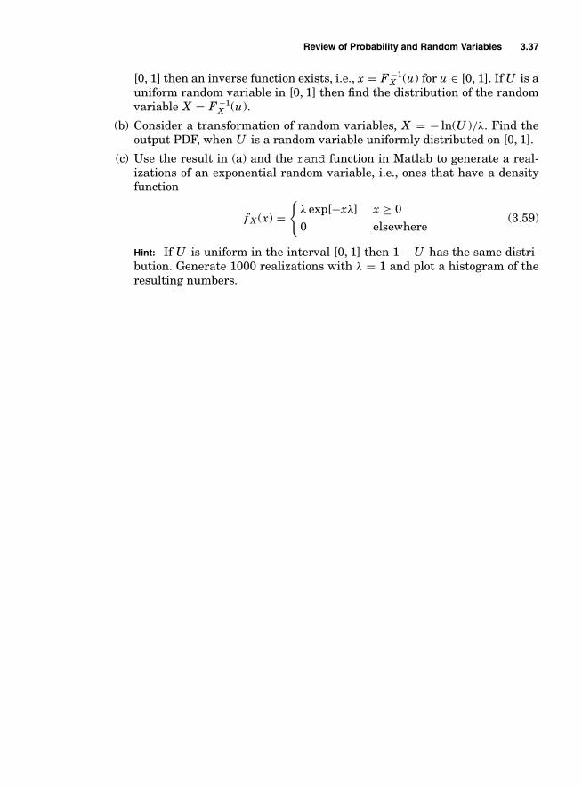
Review of Probability and Random Variables 3.37
[0, 1] then an inverse function exists, i.e., x = F −1X (u) for u ∈ [0, 1]. If U is a
uniform random variable in [0, 1] then find the distribution of the randomvariable X = F −1
X (u).
(b) Consider a transformation of random variables, X = − ln(U )/λ. Find theoutput PDF, when U is a random variable uniformly distributed on [0, 1].
(c) Use the result in (a) and the rand function in Matlab to generate a real-izations of an exponential random variable, i.e., ones that have a densityfunction
f X (x) ={
λ exp[−xλ] x ≥ 00 elsewhere
(3.59)
Hint: If U is uniform in the interval [0, 1] then 1 − U has the same distri-bution. Generate 1000 realizations with λ = 1 and plot a histogram of theresulting numbers.

This page intentionally left blank

Chapter
4Complex Baseband
Representation of BandpassSignals
4.1 Introduction
A majority of communication systems operate by modulating an informationbearing waveform onto a sinusoidal carrier. As examples, Table 4.1 lists thecarrier frequencies of various methods of electronic communication.
One can see by examining Table 4.1 that the carrier frequency of the trans-mitted signal is not the component which contains the information. Instead itis the signal modulated on the carrier which contains the information. Hencea method of characterizing a communication signal, which is independent ofthe carrier frequency, is desired. This has led communication system engineersto use a complex baseband representation of communication signals tosimplify their job. All of the communication systems mentioned in Table 4.1can be and typically are analyzed with this complex baseband representation.This chapter develops the complex baseband representation for determinis-tic signals. Other references that develop these topics well are [Pro89, PS94,Hay83, BB99]. One advantage of the complex baseband representation is sim-plicity. When communication system engineers use the complex basebandnotation, all signals are lowpass signals and the fundamental ideas behindmodulation and communication signal processing are easily developed. Alsodigital processing based receivers use the complex baseband representation indescribing the baseband processing algorithms. In fact, complex baseband rep-resentation is so prevalent in engineering systems that the most widely usedtool, Matlab, has been configured by default to process all variables in a pro-gram as complex signals. Hopefully by the time you are done with this coursethe utility of this view will be apparent.
4.1
Copyright © 2007 by The McGraw-Hill Companies. Click here for terms of use.

4.2 Chapter Four
TABLE 4.1 Carrier frequency assignments for different methodsof information transmission
Type of Transmission Center Frequency of Transmission
Telephone Modems 1600–1800 HzAM radio 530–1600 kHzCB radio 27 MHzFM radio 88–108 MHzVHF TV 178–216 MHzCellular radio 850 MHz, 1.8 GHzIndoor Wireless Networks 2.4 GHzCommercial Satellite Downlink 3.7–4.2 GHzCommercial Satellite Uplink 5.9–6.4 GHzFiber Optics 2 × 10¹⁴ Hz
4.2 Baseband Representation of Bandpass Signals
The first step in the development of a complex baseband representation is todefine a bandpass signal.
Definition 4.1 A bandpass signal, xc(t), is a signal whose one-sided energy spectrum isboth: (1) centered at a nonzero frequency, f C , and (2) does not extend in frequency tozero (DC).
The two-sided transmission bandwidth of a signal is typically denoted byBT Hertz so that the one-sided spectrum of the bandpass signal is zero ex-cept in [ fC − BT /2, fC + BT /2]. This implies that a bandpass signal satis-fies the following constraint: BT /2 < fC . Figure 4.1 illustrates a conformantbandpass energy spectrum. Since a bandpass signal, xc(t), is a physically re-alizable signal it is real valued and consequently the energy spectrum willalways be even symmetric around f = 0. The relative sizes of BT and fCare not important, only that the spectrum takes negligible values around DC.In telephone modem communications this region of negligible spectral valuesis only about 300 Hz wide, while in satellite communications it can be manygigahertz.
BT
Gxc(f )
f−fC fC
Figure 4.1 Energy spectrum of a bandpass signal.

Complex Baseband Representation of Bandpass Signals 4.3
A bandpass signal has a representation of
xc(t) = xI (t)√
2 cos(2π fct) − xQ(t)√
2 sin(2π fct) (4.1)
= xA(t)√
2 cos(2π fct + xP (t)) (4.2)
where fc is denoted the carrier frequency with fC − BT /2 ≤ fc ≤ fC + BT /2.The signal xI (t) in Eq. (4.1) is normally referred to as the in-phase (I) compo-nent of the signal and the signal xQ(t) is normally referred to as the quadrature(Q) component of the bandpass signal. xI (t) and xQ(t) are real valued lowpasssignals with a one-sided non–negligible energy spectrum no larger than BT Hz.Two items should be noted
■ The center frequency of the bandpass signal, fC , (see Figure 4.1) and thecarrier frequency, fc are not always the same. While fc can theoretically takea continuum of values in Eq. (4.1), in most applications an obvious value offc will give the simplest representation1.
■ The√
2 term is included in the definition of the bandpass signal to ensure thatthe bandpass signal and the baseband signal have the same power/energy.This will become apparent in Section 4.4.
The carrier signal is normally thought of as the cosine term, hence the Icomponent is in-phase with the carrier. Likewise the sine term is 90◦ out-of-phase (in quadrature) with the cosine or carrier term, hence the Q componentis quadrature to the carrier. Equation (4.1) is known as the canonical form of abandpass signal. Equation (4.2) is the amplitude and phase form of the band-pass signal, where xA(t) is the amplitude of the signal and xP (t) is the phaseof the signal. A bandpass signal has two degrees of freedom. A communicationengineer can use either the I/Q representation or the amplitude and phase rep-resentation to denote a bandpass signal. The transformations between the tworepresentations are given by
xA(t) =√
xI (t)2 + xQ(t)2 xP (t) = tan−1[xQ(t), xI (t)] (4.3)
and
xI (t) = xA(t) cos(xP (t)) xQ(t) = xA(t) sin(xP (t)) (4.4)
Note that the inverse tangent function in Eq. (4.3) has a range of [−π, π ] (i.e.,both the sign of xI (t) and xQ(t) and the ratio of xI (t) and xQ(t) are neededto evaluate the function). This inverse tangent function is different than thesingle argument function that is on most calculators. The particulars of thecommunication design analysis determine which form for the bandpass signalis most applicable.
1This idea will become more obvious in Chapter 6.

4.4 Chapter Four
A complex valued signal, denoted the complex envelope, is defined as
xz(t) = xI (t) + j xQ(t) = xA(t) exp[ j xP (t)]
The original bandpass signal can be obtained from the complex envelope by
xc(t) =√
2[xz(t) exp[ j 2π fct]]. (4.5)
Since the complex exponential only determines the carrier frequency, thecomplex signal xz(t) contains all the information in xc(t). Using this complexbaseband representation of bandpass signals greatly simplifies the notation forcommunication system analysis. As you progress through the text hopefullythe additional simplicity provided by the complex envelope representation willbecome evident.
EXAMPLE 4.1Consider the bandpass signal
xc(t) = 2 cos(2π fmt)√
2 cos(2π fct) − sin(2π fmt)√
2 sin(2π fct)
where fm < fc. A plot of this bandpass signal is seen in Figure 4.2 with fc = 10 fm.Obviously we have
xI (t) = 2 cos(2π fmt) xQ(t) = sin(2π fmt)
and
xz(t) = 2 cos(2π fmt) + j sin(2π fmt)
The amplitude and phase can be computed as
xA(t) =√
1 + 3 cos2(2π fmt) xP (t) = tan−1[sin(2π fmt), 2 cos(2π fmt)].
A plot of the amplitude and phase of this signal is seen in Figure 4.3.
As an interesting historical note, the communications field did not always uti-lize the complex baseband notation. Originally, communication theorist adoptedthe “analytical signal” denoted
xan(t) = xz(t) exp[ j 2π fct] (4.6)
as a way to understand communication signals. This complex analytical signalwas viewed as useful since it was more mathematically tractable and yet cap-ture all the characteristics of communications signals. Slowly over time the fieldcame to realize that the important characteristics of a communication wave-form are captured by the complex envelope, xz(t). An early tutorial paper onthe complex analytical signal is given in [Bed62]. Hence the complex envelope

Complex Baseband Representation of Bandpass Signals 4.5
−3
−2
−1
0
1
2
3
0 0.5 1 0.5 2
x c(t
)
Normalized Time, fmt
Figure 4.2 Plot of the bandpass signal for Example 4.1.
0
0.5
1
1.5
2
−150
−100
−50
0
50
100
150
Amplitude Phase
0 0.5 1 0.5 2
Am
plitu
de
Phas
e, d
egre
es
Normalized time
Figure 4.3 Plot of the amplitude and phase for Example 4.1.

4.6 Chapter Four
LPF
LPF
Σ+
Complex Baseband toBandpass Conversion
Bandpass to ComplexBaseband Conversion
π 2 π 2
2 2cos πf tc( )
xI(t)
−
−xQ(t)
x1(t)
x2(t)
xI(t)
xQ(t)
xc(t)2 2cos πf tc( )
Figure 4.4 Schemes for converting between complex baseband and bandpass representations. Notethat the LPF simply removes the double frequency term associated with the down conversion.
representation of bandpass signals is an excellent example of the evolution of anengineering tool where no one person can really be ascribed to the “invention.”
The next item to consider is methods to translate between a bandpass sig-nal and a complex envelope signal. Figure 4.4 shows the block diagram of thetranslation between a complex envelope and a bandpass signal and vice versa.Basically a bandpass signal is generated from its I and Q components in astraightforward fashion corresponding to Eq. (4.1). Likewise a complex enve-lope signal is generated from the bandpass signal with a similar architecture.Bandpass to baseband downconversion can be understood by using trigonomet-ric identities to give
x1(t) = xc(t)√
2 cos(2π fct) = xI (t) + xI (t) cos(4π fct) − xQ(t) sin(4π fct)(4.7)
x2(t) = xc(t)√
2 sin(2π fct) = −xQ(t) + xQ(t) cos(4π fct) + xI (t) sin(4π fct)
In Figure 4.4 the lowpass filters remove the 2 fc terms in Eq. (4.7). Note inFigure 4.4 the boxes with π/2 are phase shifters (i.e., cos(θ − π/2) = sin(θ ))typically implemented with delay elements. The structure in Figure 4.4 is fun-damental to the study of all carrier modulation techniques.
4.3 Visualization of Complex Envelopes
The complex envelope is a signal that is a complex function of time. Conse-quently, the complex envelope needs to be characterized in three dimensions(time, in-phase, and quadrature). For example, the complex envelope given as
xz(t) = exp[ j 2π fmt] = cos(2π fmt) + j sin(2π fmt) (4.8)
can be represented as a three dimensional plot as shown in Figure 4.5(a). It isoften difficult to comprehend all that is going on in a three-dimensional plot

Complex Baseband Representation of Bandpass Signals 4.7
00.5
11.5
22.5 3
(a) The three dimensional plot.
−1−0.5
00.5
1−1
−0.5
0
0.5
1
xI(t)Time, t/fm
x Q(t
)
−1 −0.8 −0.6 −0.4 −0.2 0
(b) The projection onto the xI(t), xQ(t) plane.
0.2 0.4 0.6 0.8 1−1
−0.8
−0.6
−0.4
−0.2
0
0.2
0.4
0.6
0.8
1
xI(t)
x Q(t
)
Figure 4.5 Plots of a complex exponential.
when the complex envelope is a typical communication signal hence communi-cation engineers often project these signals into two dimensions. Examples ofthis two-dimensional projection are shown in Figure 4.5(b) (xI (t) versus xQ(t)),Figure 4.6(a) (t versus xI (t)), and Figure 4.6(b) (t versus xQ(t)). All of thesemethods of viewing and visualizing a complex envelope signal are used in en-gineering practice.
The vector diagram is the two-dimensional projection, where xI (t) is plottedversus xQ(t). The vector diagram represents the time trajectory of the complexenvelope, xz(t), in the complex plane. This vector diagram often gives signifi-cant insight into the performance or characteristics of a communication system
0 0.5 1 1.5 2 2.5 3−1
−0.8
−0.6
−0.4
−0.2
0
0.2
0.4
0.6
0.8
1
Time, t/fm
(a) The projection onto the t, xI(t) plane.
x I(t
)
−1
−0.8
−0.6
−0.4
−0.2
0
0.2
0.4
0.6
0.8
1
0 0.5 1 1.5 2 2.5 3Time, t/fm
(b) The projection onto the t, xQ(t) plane.
x Q(t
)
Figure 4.6 Plots of the two time functions.

4.8 Chapter Four
and it will be used often in future sections of this text. The vector diagram firstgained utility in the days when the standard tool for examining the time domaincharacteristics of a communication signal was the dual channel analog oscillo-scope. To produce a vector diagram with a dual channel oscilloscope, xI (t) is putinto one channel and xQ(t) is put into the second channel and the scope is con-figured to plot channel 1 versus channel 2. Since early test instruments couldsimply generate this visualization, the vector diagram has traditionally foundutility in engineering practice. In fact, modern communication test equipmentlike the Agilent 89600 vector signal analyzer are based around the characteri-zation of the complex envelope and have the ability to measure vector diagramsof bandpass signals.
EXAMPLE 4.2The vector diagram for the bandpass signal given in Example 4.1 is shown in Figure 4.7.It should be noted that the point xz(t) = (2, 0) corresponds to time t = n/ fm where n is an
tn
f fm m
= +3
4
tn
fm
=
−1
−1.5
−1
−0.5
0
0.5
1
1.5
2
x Q(t
)
−2 −1.5 −1 −0.5 0 0.5 1 1.5 2
xI(t)
Figure 4.7 The vector diagram for the bandpass signal in Example 4.1.

Complex Baseband Representation of Bandpass Signals 4.9
integer, e.g., 2 cos(2πn) = 2 and sin(2πn) = 0. Likewise t = n/ fm + 1/(4 fm) correspondsto the point xz(t) = (0, 1).
4.4 Spectral Characteristics of the Complex Envelope
4.4.1 Basics
It is of interest to derive the spectral representation of the complex basebandsignal, xz(t), and compare it to the spectral representation of the bandpasssignal, xc(t). Assuming xz(t) is an energy signal, the Fourier transform of xz(t)is given by
Xz(f ) = X I (f ) + j X Q(f ) (4.9)
where X I (f ) and X Q(f ) are the Fourier transform of xI (t) and xQ(t), respec-tively, and the energy spectrum is given by
Gxz(f ) = |Xz(f )|2 = GxI (f ) + GxQ (f ) + 2�[X I (f )X ∗Q(f )] (4.10)
where GxI (f ) and GxQ (f ) are the energy spectrum of xI (t) and xQ(t), respectively.The signals xI (t) and xQ(t) are lowpass signals with a one-sided bandwidth ofless than BT /2 so consequently Xz(f ) and Gxz(f ) can only take nonzero valuesfor | f | < BT /2.
EXAMPLE 4.3Consider the case when xI (t) is set to be the message signal from Example 2.3 (com-puter generated voice saying “bingo”) and xQ(t) = cos(2000πt). X I (f ) will be a lowpassspectrum with a bandwidth of 2500 Hz while X Q(f ) will have two impulses locatedat ±1000 Hz. Figure 4.8 shows the measured complex envelope energy spectrum forthese lowpass signals. The complex envelope energy spectrum has a relation to thevoice spectrum and the sinusoidal spectrum exactly as predicted in Eq. (4.10). Notehere BT = 5000 Hz.
Equation (4.9) gives a simple way to transform between the lowpass signalspectrums to the complex envelope spectrum. A similar simple formula existsfor the opposite transformation. Note that xI (t) and xQ(t) are both real signalsso that X I (f ) and X Q(f ) are Hermitian symmetric functions of frequency. It isstraightforward to show
Xz(− f ) = X ∗I (f ) + j X ∗
Q(f )(4.11)
X ∗z (− f ) = X I (f ) − j X Q(f )

4.10 Chapter Four
−5000 −4000 −3000 −2000 −1000 0 1000 2000 3000 4000 5000−70
−60
−50
−40
−30
−20
−10
0
Frequency, f, Hz
Gy z(f
)
Figure 4.8 The energy spectrum resulting from xI (t) being a computer generated voice signaland xQ(t) being a sinusoid.
This leads directly to
X I (f ) = Xz(f ) + X ∗z (− f )
2(4.12)
X Q(f ) = Xz(f ) − X ∗z (− f )
j 2
Since xz(t) is a complex signal, in general, the energy spectrum, Gxz(f ), hasnone of the usual properties of real signal spectra. Real signals have a spectralmagnitude that is an even function of f and a spectral phase that is an oddfunction of f . Complex envelopes spectra are not so restricted.
An analogous derivation produces the spectral characteristics of the bandpasssignal. Examining Eq. (4.1) and using the Frequency Translation Theorem ofthe Fourier transform, the Fourier transform of the bandpass signal, xc(t), isexpressed as
Xc(f ) =[
1√2
X I (f − fc) + 1√2
X I (f + fc)]
−[
1√2 j
X Q(f − fc) − 1√2 j
X Q(f + fc)]

Complex Baseband Representation of Bandpass Signals 4.11
This can be rearranged to give
Xc(f ) =[
X I (f − fc) + j X Q(f − fc)√2
]+[
X I (f + fc) − j X Q(f + fc)√2
](4.13)
Using Eq. (4.11) in Eq. (4.13) gives
Xc(f ) = 1√2
Xz(f − fc) + 1√2
X ∗z (− f − fc) (4.14)
This is a very fundamental result. Equation (4.14) states that the Fouriertransform of a bandpass signal is simply derived from the spectrum of thecomplex envelope. For positive values of f , Xc(f ) is obtained by translatingXz(f ) to fc and scaling the amplitude by 1/
√2. For negative values of f , Xc(f )
is obtained by flipping Xz(f ) around the origin, taking the complex conjugate,translating the result to − fc, and scaling the amplitude by 1/
√2 . This also
demonstrates that if Xc(f ) only takes values when the absolute value of f is in[ fc − BT /2, fc + BT /2], then Xz(f ) only takes values in [−BT /2, BT /2]. Theenergy spectrum of xc(t) can also be expressed in terms of the energy spectrumof xz(t) as
Gxc (f ) = 12
Gxz(f − fc) + 12
Gxz(− f − fc) (4.15)
Since Exc = ∫∞−∞ Gxc (f ) df = ∫∞
−∞ Gxz(f ) df, Eq. (4.15) guarantees that the en-ergy of the complex envelope is identical to the energy of the bandpass signal.Additionally, Eq. (4.15) guarantees that the energy spectrum of the bandpasssignal is an even function of frequency as it should be for a real signal. Consid-ering these results, the spectrum of the complex envelope of the signal shown inFigure 4.1 will have a form shown in Figure 4.9 when fc = fC . Other values offc would produce a different but equivalent complex envelope representation.This discussion of the spectral characteristics of xc(t) and xz(t) should reinforcethe idea that the complex envelope contains all the information in a bandpasswaveform.
Gxz( f )
f
BT
Figure 4.9 The complex envelopeenergy spectrum of the bandpasssignal in Figure 4.1 with fc = fC .

4.12 Chapter Four
EXAMPLE 4.4(Example 4.1 cont.)
xI (t) = 2 cos(2π fmt) xQ(t) = sin(2π fmt)
X I (f ) = δ(f − fm) + δ(f + fm) X Q(f ) = 12 j
δ(f − fm) − 12 j
δ(f + fm)
Xz(f ) = X I (f ) + j X Q(f ) = 1.5δ(f − fm) + 0.5δ(f + fm)
and using Eq. (4.14) gives the bandpass signal spectrum as
Xc(f ) = 1.5√2
δ(f − fc − fm) + 1
2√
2δ(f − fc + fm) + 1.5√
2δ(f + fc + fm) + 1
2√
2δ(f + fc − fm)
Note in this example BT = 2 fm
EXAMPLE 4.5For the complex envelope derived in Example 4.3 the measured bandpass energy spec-trum for fc = 7000 Hz is shown in Figure 4.10. Again the measured output is exactlypredicted by Eq. (4.15). In this example we have BT = 5000 Hz.
× 104
−70
−60
−50
−40
−30
−20
−10
0
Gy C
(f)
−1 −0.8 −0.6 −0.4 −0.2 0 0.2 0.4 0.6 0.8 1Frequency, f, Hz
Figure 4.10 The bandpass spectrum corresponding to Figure 4.8. BT = 5000 Hz.

Complex Baseband Representation of Bandpass Signals 4.13
4.4.2 Bandwidth of Bandpass Signals
The ideas of bandwidth of a signal extend in an obvious way to bandpass signals.Recall engineers define bandwidth as being the amount of positive spectrumthat a signal occupies. For bandpass energy signals we have the following twodefinitions that are analogous to the bandwidth definitions in Chapter 2.
Definition 4.2 If a signal xc(t) has an energy spectrum Gxc (f ) then BX is determined as
10 log(
maxf
Gxc (f )) = X + 10 log(Gxc (f 1)) (4.16)
where Gxc (f 1) > Gxc (f ) for 0 < f < f 1 and
10 log(
maxf
Gxc (f )) = X + 10 log(Gxc (f 2)) (4.17)
where Gxc (f 2) > Gxc (f ) for f > f 2 where f 2 − f 1 = BX .
Definition 4.3 If a signal xc(t) has an energy spectrum Gxc (f ) then BP = min(f 2 − f 1)such that
P =2∫ f 2
f 1Gxc (f ) df
Exc
(4.18)
where f 2 > f 1.
Note the reason for the factor of 2 in Eq. (4.21) is that half of the energy of thebandpass signal is associated with positive frequencies and half of the energyis associated with negative frequencies.
Again, for bandpass power signals similar ideas hold with Gxc (f ) being re-placed with Sxc (f , T ).
Definition 4.4 If a signal xc(t) has a sampled power spectral density Sxc (f , T m) (seeEq. (2.56)) then BX is determined as
10 log(
maxf
Sxc (f , T m)) = X + 10 log(Sxc (f 1, T m)) (4.19)
where Sxc (f 1, T m) > Sxc (f , T m) for 0 < f < f 1 and
10 log(
maxf
Sxc (f , T m)) = X + 10 log(Sxc (f 2, T m)) (4.20)
where Sxc (f 2, T m) > Sxc (f , T m) for f > f 2 where f 2 − f 1 = BX .
Definition 4.5 If a signal xc(t) has an power spectrum Sxc (f , T m) then BP = min(f 2−f 1)such that
P =2∫ f 2
f 1Sxc (f , T m) df
Pxc (T m)(4.21)
where f 2 > f 1 and Pxc (T m) is defined in Eq. (2.57).

4.14 Chapter Four
4.5 Power of Carrier Modulated Signals
The output power of a carrier modulated signal is often important in evaluatingthe trade-offs between analog communication options. For generality of theexposition in this text, power will be computed as a time average power. Thetime average power is defined as
Pxc = limT m→∞
1T m
∫ T m/2
−T m/2x2
c (t)dt (4.22)
Using the Rayleigh energy theorem and Eq. (2.56) the time average power of abandpass modulated signal is
Pxc = limT m→∞
∫ ∞
−∞SXc (f , T m) df (4.23)
Using the power spectrum analog to Eq. (4.15) gives
Pxc = limT m→∞
1T m
∫ T m/2
−T m/2|xz(t)|2dt = Pxz (4.24)
Hence we have shown that the power contained in a carrier modulated signalis exactly the power in the complex envelope. This result is the main reasonwhy the notation used in this text uses the
√2 term in the carrier terms.
4.6 Linear Systems and Bandpass Signals
This section discusses methods for calculating the output of a linear, time-invariant (LTI) filter with a bandpass input signal using complex envelopes.Linear system outputs are characterized by the convolution integral given as
yc(t) =∫ ∞
−∞xc(τ )h(t − τ )dτ (4.25)
where h(t) is the impulse response of the filter. Since the input signal is band-pass, the effects of an arbitrary filter, h(t), in Eq. (4.25) can be modeled with anequivalent bandpass filter, hc(t), with no loss in generality. The bandpass filter,Hc(f ), only needs to equal the true filter, H (f ) over the frequency support of thebandpass signal and the two filters need not be equal otherwise. Because of thischaracterization the bandpass filter is often simpler to model (and to simulate).
EXAMPLE 4.6For example consider the lowpass filter given in Figure 4.11(a). Since the bandpasssignal only has a nonzero spectrum in a bandwidth of BT around the carrier frequency,fc, the bandpass filter shown in Figure 4.11(b) would be input–output equivalent to thefilter in Figure 4.11(a).
This bandpass LTI system also has a canonical representation given as
hc(t) = 2hI (t) cos(2π fct) − 2hQ(t) sin(2π fct) (4.26)

Complex Baseband Representation of Bandpass Signals 4.15
H( f )
A
(a) A low pass filter. (b) An input/output equivalent bandpass filter.
fc−fcf
BT
Hc( f )
fc−fcf
A
Figure 4.11 An example of a filter and its bandpass equivalent filter.
The complex envelope for this bandpass impulse response and transfer functionassociated with this complex envelope are given by
hz(t) = hI (t) + j hQ(t) Hz(f ) = HI (f ) + j HQ(f )
where the bandpass system impulse response is
hc(t) = 2[hz(t) exp[ j 2π fct]]
The representation of the bandpass system in Eq. (4.26) has a constant factorof
√2 difference from the bandpass signal representation of Eq. (4.1). This
factor results because the system response at baseband and at bandpass shouldbe identical. This notational convenience permits a simpler expression for thesystem output (as is shown shortly). Using similar techniques as in Section 4.4,the transfer function is expressed as
Hc(f ) = Hz(f − fc) + H ∗z (− f − fc) (4.27)
EXAMPLE 4.7Consider the signal
xc(t) = (cos(2π fmt) + cos(6π fmt))√
2 cos(2π fct) − (sin(2π fmt)
+ sin(6π fmt))√
2 sin(2π fct) (4.28)
that is input into a bandpass filter with a transfer function of
Hc(f ) ={
2 fc − 2 fm ≤ | f | ≤ fc + 2 fm
0 elsewhere(4.29)
Since the frequency domain representation of xc(t) is
Xc(f ) = 1√2
[δ(f − (fc + fm)) + δ(f − (fc + 3 fm) + δ(f + (fc + fm)
+ δ(f + (fc + 3 fm)] (4.30)

4.16 Chapter Four
the output bandpass signal will have the frequency domain representation of
Yc(f ) = 2√2
[δ(f − (fc + fm) + δ(f + (fc + fm)] (4.31)
The complex envelopes of the input and output signals are
xz(t) = exp[ j 2π fmt] + exp[ j 6π fmt] yz(t) = 2 exp[ j 2π fmt] (4.32)
consequently it makes sense to have
Hz(f ) ={
2 | f | ≤ 2 fm
0 elsewhere(4.33)
and Hc(f ) = Hz(f − fc) + H∗z (− f − fc).
Equations (4.27) and (4.14) combined with the convolution theorem of theFourier transform produce an expression for the Fourier transform of yc(t)given as
Yc(f ) = Xc(f )Hc(f ) = 1√2
[Xz(f − fc) + X ∗z (− f − fc)][Hz(f − fc)
+ H ∗z (− f − fc)]
Since both Xz(f ) and Hz(f ) only take nonzero values in [−BT /2, BT /2], thecross terms in this expression will be zero and Yc(f ) is given by
Yc(f ) = 1√2
[Xz(f − fc)Hz(f − fc) + X ∗z (− f − fc)H ∗
z (− f − fc)] (4.34)
Since yc(t) will also be a bandpass signal, it will also have a complex basebandrepresentation. A comparison of Eq. (4.34) with Eq. (4.14) demonstrates theFourier transform of the complex envelope of yc(t), yz(t), is given as
Yz(f ) = Xz(f )Hz(f )
Linear system theory produces the desired form
yz(t) =∫ ∞
−∞xz(τ )hz(t − τ )d τ = xz(t) ∗ hz(t) (4.35)
EXAMPLE 4.8(Example 4.1 cont.) The input signal and Fourier transform are
xz(t) = 2 cos(2π fmt) + j sin(2π fmt) Xz(f ) = 1.5δ(f − fm) + 0.5δ(f + fm)
Assume a bandpass filter with
HI (f ) ={
2 −2 fm ≤ f ≤ 2 fm
0 elsewhereHQ(f ) =
⎧⎪⎪⎪⎨⎪⎪⎪⎩
j ffm
−fm ≤ f ≤ fm
j fm ≤ f ≤ 2 fm
− j −2 fm ≤ f ≤ −fm
0 elsewhere
(4.36)

Complex Baseband Representation of Bandpass Signals 4.17
This produces
Hz(f ) =
⎧⎪⎪⎪⎨⎪⎪⎪⎩
2 − ffm
−fm ≤ f ≤ fm
1 fm ≤ f ≤ 2 fm
3 −2 fm ≤ f ≤ −fm
0 elsewhere
(4.37)
and now the Fourier transform of the complex envelope of the filter output is
Yz(f ) = Hz(f )Xz(f ) = 1.5δ(f − fm) + 1.5δ(f + fm) (4.38)
The complex envelope and bandpass signal are given as
yz(t) = 3 cos(2π fmt) yc(t) = 3 cos(2π fmt)√
2 cos(2π fct) (4.39)
In other words, convolving the complex envelope of the input signal with thecomplex envelope of the filter response produces the complex envelope of theoutput signal. The different scale factor was introduced in Eq. (4.26) so thatEq. (4.35) would have a familiar form. This result is significant since yc(t) canbe derived by computing a convolution of baseband (complex) signals, which isgenerally much simpler than computing the bandpass convolution. Since xz(t)and hz(t) are complex, yz(t) is given in terms of the I/Q components as
yz(t) = yI (t) + j yQ(t) = [xI (t) ∗ hI (t) − xQ(t) ∗ hQ(t)]
+ j [xI (t) ∗ hQ(t) + xQ(t) ∗ hI (t)]
Figure 4.12 shows the lowpass equivalent model of a bandpass system. Thetwo biggest advantages of using the complex baseband representation are thatit simplifies the analysis of communication systems and permits accurate dig-ital computer simulation of filters and the effects on communication systemsperformance.
+
−
+
+
Σ
Σ yQ(t )
hQ(t )
hQ(t )
xQ(t )
hI(t )
hI(t )xI(t )
yI (t )
Figure 4.12 Block diagram illustrating the relation between the input andoutput complex envelope of bandpass signals for a linear time invariantsystem.
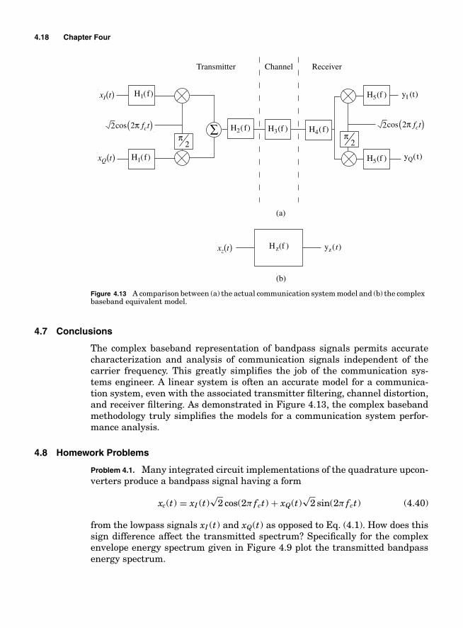
4.18 Chapter Four
∑
H1(f)
H3(f )
Transmitter Channel Receiver
H4(f)
H5(f )
yQ(t)
yI (t)
H1(f) H5(f )
H2(f)
xI(t)
xQ(t)
z(t) Hz(f ) yz(t)
(a)
(b)
xI t( )
xQ t( )
xz t( )
π2
π2
cos π fct( )2 cos π fct( )22 2
Figure 4.13 A comparison between (a) the actual communication system model and (b) the complexbaseband equivalent model.
4.7 Conclusions
The complex baseband representation of bandpass signals permits accuratecharacterization and analysis of communication signals independent of thecarrier frequency. This greatly simplifies the job of the communication sys-tems engineer. A linear system is often an accurate model for a communica-tion system, even with the associated transmitter filtering, channel distortion,and receiver filtering. As demonstrated in Figure 4.13, the complex basebandmethodology truly simplifies the models for a communication system perfor-mance analysis.
4.8 Homework Problems
Problem 4.1. Many integrated circuit implementations of the quadrature upcon-verters produce a bandpass signal having a form
xc(t) = xI (t)√
2 cos(2π fct) + xQ(t)√
2 sin(2π fct) (4.40)
from the lowpass signals xI (t) and xQ(t) as opposed to Eq. (4.1). How does thissign difference affect the transmitted spectrum? Specifically for the complexenvelope energy spectrum given in Figure 4.9 plot the transmitted bandpassenergy spectrum.

Complex Baseband Representation of Bandpass Signals 4.19
Problem 4.2. Find the form of xI (t) and xQ(t) for the following xc(t)
(a) xc(t) = sin(2π(fc − fm)t)
(b) xc(t) = cos(2π(fc + fm)t)
(c) xc(t) = cos(2π fct + φp)
Problem 4.3. If the lowpass components for a bandpass signal are of the form
xI (t) = 12 cos(6πt) + 3 cos(10πt)
and
xQ(t) = 2 sin(6πt) + 3 sin(10πt)
(a) Calculate the Fourier series of xI (t) and xQ(t).
(b) Calculate the Fourier series of xz(t).
(c) Assuming fc = 40 Hz calculate the Fourier series of xc(t).
(d) Calculate and plot xA(t). Computer might be useful.
(e) Calculate and plot xP (t). Computer might be useful.
Problem 4.4. A bandpass filter has the following complex envelope representationfor the impulse response
hz(t) =⎧⎨⎩
2(
12 exp[
− t2
])+ j 2(
14 exp[
− t4
])t ≥ 0
0 elsewhere(4.41)
(a) Calculate Hz(f ).
Hint: The transforms you need are in a table somewhere.
(b) With xz(t) from Problem 4.3 as the input, calculate the Fourier series forthe filter output, yz(t).
(c) Plot the output amplitude, yA(t), and phase, yP (t).
(d) Plot the resulting bandpass signal, yc(t) using fc = 40 Hz.
Problem 4.5. The picture of a color television set proposed by the National Tele-vision System Committee (NTSC) is composed by scanning in a grid patternacross the screen. The scan is made up of three independent beams (red, green,and blue). These independent beams can be combined to make any color at aparticular position. In order to make the original color transmission compati-ble with black and white televisions the three color signals (xr (t), xg(t), xb(t))are transformed into a luminance signal (black and white level), xL(t), and twoindependent chrominance signals, xI (t) and xQ(t). These chrominance signalsare modulated onto a carrier of 3.58 MHz to produce a bandpass signal fortransmission. A commonly used tool for video engineers to understand thesecoloring patterns is the vectorscope representation shown in Figure 4.14.

4.20 Chapter Four
x tI ( )
x tQ( )
• Red
• Yellow
• Green
• Cyan
• Blue
• Magenta
0 64 13 7°. exp .j[ ]
0 45 77°. exp j[ ]
0 59 151°. exp j[ ]
0 64 193°. exp j[ ]
0 45 257°. exp j[ ]
0 59 331°. exp j[ ]
Figure 4.14 Vector scope representation of the complex envelopeof the 3.58 MHz chrominance carrier.
(a) If the video picture is making a smooth transition from a blue color (at t =0) to green color (at t = 1), make a plot of the waveforms xI (t) and xQ(t).
(b) Plot xI (t) and xQ(t) that would represent a scan across a red and greenstriped area. For consistency in the answers assume the red starts at t = 0and extends to t = 1, the green starts at t = 1+ and extends to t = 2, · · ·.
Problem 4.6. Consider two lowpass spectra, X I (f ) and X Q(f ) in Figure 4.15 andsketch the energy spectrum of the complex envelope, Gxz(f ).
Im X fI( )[ ] = 0
f1f1
− f1
A A
−A
Re X fQ ( )[ ] = 0
−f1
Im X fQ( )[ ]Re X fI( )[ ]
Figure 4.15 Two lowpass Fourier transforms.

Complex Baseband Representation of Bandpass Signals 4.21
2 cos 2πfct( )
2 cos − π 2) = 2 sinπ 2 2πfct( )2πfc t(
2 cos 2πfct( )
Figure 4.16 Sine and cosine generator.
Problem 4.7. (Design Problem) A key component in the quadrature up/downconverter is the generator of the sine and cosine functions. This processing isrepresented in Figure 4.16 as a shift in the phase by 90◦ of a carrier signal.This function is done in digital processing in a trivial way but if the carrieris generated by an analog source the implementation is more tricky. Showthat this phase shift can be generated with a time delay as in Figure 4.17.If the carrier frequency is 100 MHz, find the value of the delay to achieve the90◦ shift.
Problem 4.8. The lowpass signals, xI (t) and xQ(t), which comprise a bandpasssignal are given in Figure 4.18.
(a) Give the form of xc(t), the bandpass signal with a carrier frequency fc, usingxI (t) and xQ(t).
(b) Find the amplitude, xA(t), and the phase, xP (t), of the bandpass signal.
(c) Give the simplest form for the bandpass signal over [2T , 3T ].
Problem 4.9. The amplitude and phase of a bandpass signal is plotted inFigure 4.19. Plot the in-phase and quadrature signals of this basebandrepresentation of a bandpass signal.
Problem 4.10. The block diagram in Figure 4.20 shows a cascade of a quadra-ture upconverter and a quadrature downconverter where the phases of the two(transmit and receive) carriers are not the same. Show that yz(t) = yI (t) +j yQ(t) = xz(t) exp[− j θ (t)]. Specifically consider the case when the frequenciesof the two carriers are not the same and compute the resulting output energyspectrum GYz(f ).
2 cos 2πfct( )
2 cos − τ)τ )2π fc t( (
2 cos 2πfct( )
Figure 4.17 Sine and cosine generator implementation for analog signals.

4.22 Chapter Four
x tI( )
x tQ( )
1
1
−1
−1
T 2T 3T 4T t
t4T3T2TT
Figure 4.18 xI (t) and xQ(t).
1
T 2T 3T 4T
T 2T 3T 4T
π
π/2
−π/2
−π
xA t( )
xP t( )t
t
Figure 4.19 The amplitude and phase of a bandpass signal.
LPF
xc(t)
LPF
∑+
2 cos 2πfct( )
xI t( )
xQ t( )
−+ θ(t))
yI t( )
π/2 π/2−yQ t( )
2cos 2πfct(
−
Figure 4.20 A downconverter with a phase offset.

Complex Baseband Representation of Bandpass Signals 4.23
Problem 4.11. A periodic real signal of bandwidth W and period T is xI (t) andxQ(t) = 0 for a bandpass signal of carrier frequency fc > W .
(a) Can the resulting bandpass signal, xc(t), be periodic with a period of Tc < T ?If yes, give an example.
(b) Can the resulting bandpass signal, xc(t), be periodic with a period of Tc > T ?If yes, give an example.
(c) Can the resulting bandpass signal, xc(t), be periodic with a period of Tc = T ?If yes, give an example.
(d) Can the resulting bandpass signal, xc(t), be aperiodic? If yes, give anexample.
Problem 4.12. In communication systems bandpass signals are often processedin digital processors. To accomplish the processing, the bandpass signal mustfirst be converted from an analog signal to a digital signal. For this problemassume this is done by ideal sampling. Assume the sampling frequency, f s, isset at four times the carrier frequency.
(a) Under what conditions on the complex envelope will this sampling rate begreater than the Nyquist sampling rate (see Section 2.4.1) for the bandpasssignal?
(b) Give the values for the bandpass signal samples for xc(0), xc( 14 fc
), xc( 24 fc
),xc( 3
4 fc), and xc( 4
4 fc).
(c) By examining the results in (b) can you postulate a simple way to down-convert the analog signal when f s = 4 fc and produce xI (t) and xQ(t)? Thissimple idea is frequently used in engineering practice and is known as f s/4downconversion.
Problem 4.13. A common implementation problem that occurs in an I/Q upcon-verter is that the sine carrier is not exactly 90◦ out of phase with the cosinecarrier. This situation is depicted in Figure 4.21.
∑+
cos 2πfct( )
xI t( )
xc t( )
xQ t( )
−π/2 + θ
~
~
2
Figure 4.21 The block diagram for Problem 4.13.

4.24 Chapter Four
Figure 4.22 An airborne air traffic control radar example.
(a) What is the actual complex envelope, xz(t), produced by this implementationas a function of xI (t), xQ(t), and θ?
(b) Often in communication systems it is possible to correct this implementationerror by preprocessing the baseband signals. If the desired output complexenvelope was xz(t) = xI (t) + j xQ(t), what should xI (t) and xQ(t) be set toas a function of xI (t), xQ(t), and θ to achieve the desired complex envelopewith this implementation?
Problem 4.14. A commercial airliner is flying 15,000 feet above the ground andpointing its radar down to aid traffic control. A second plane is just leaving therunway as shown in Figure 4.22. The transmitted waveform is just a carriertone, xz(t) = 1 or xc(t) = √
2 cos(2π fct).The received signal return at the radar receiver input has the form
yc(t) = AP
√2 cos(2π(fc + f P )t + θP ) + AG
√2 cos(2π(fc + f G)t + θG) (4.42)
where the P subscript refers to the signal returns from the plane taking off andthe G subscript refers to the signal returns from the ground. The frequency shiftis due to the Doppler effect you learned about in your physics classes.
(a) Why does the radar signal bouncing off the ground (obviously stationary)produce a Doppler frequency shift?
(b) Give the complex baseband form of this received signal.
(c) Assume the radar receiver has a complex baseband impulse response of
hz(t) = δ(t) + βδ(t − T ) (4.43)
where β is a possibly complex constant, find the value of β which eliminatesthe returns from the ground at the output of the receiver. This system was acommon feature in early radar systems and has the common name MovingTarget Indicator (MTI) as stationary target responses will be canceled inthe filter given in Eq. (4.43).
Modern air traffic control radars are more sophisticated than this problemsuggests. An important point of this problem is that radar and communicationsystems are similar in many ways and use the same analytical techniques fordesign.

Complex Baseband Representation of Bandpass Signals 4.25
hz t( )
τd exp j2πf0 t−τd( )[ ]
yz t( )exp j2πf0t[ ]
Figure 4.23 The block diagram for Problem 4.15.
Problem 4.15. A baseband signal (a complex exponential) and two linear systemsare shown in Figure 4.23. The top linear system in Figure 4.23 has an impulseresponse of
hz(t) =
⎧⎪⎨⎪⎩
1√Tp
0 ≤ t ≤ Tp
0 elsewhere(4.44)
The bottom linear system in Figure 4.23 is an ideal delay element (i.e., yz(t) =xz(t − τd )).
(a) Give the bandpass frequency response Hc(f ).
(b) What is the input power? Compute yz(t).
(c) Select a delay, τd , in the bottom system in Figure 4.23 such that arg[yz(t)] =2π f 0(t − τd ) for all f 0.
(d) What is the output power as a function of f 0, Pyz(f 0)?
(e) How large can f 0 be before the output power, Pyz(f 0), is reduced by 10 dBcompared to the output power when f 0 = 0, Pyz(0)?
Problem 4.16. The following bandpass filter has been implemented in a commu-nication system that you have been tasked to simulate
Hc(f ) =
⎧⎪⎪⎪⎪⎪⎪⎪⎪⎪⎪⎪⎨⎪⎪⎪⎪⎪⎪⎪⎪⎪⎪⎪⎩
1 fc + 7500 ≤ | f | ≤ fc + 10000
2 fc + 2500 ≤ | f | < fc + 750043
fc ≤ | f | < fc + 2500
34
fc − 2500 ≤ | f | < fc
0 elsewhere
(4.45)
You know because of your great engineering education that it will be mucheasier to simulate the system using complex envelope representation.
(a) Find Hz(f ).
(b) Find HI (f ) and HQ(f ).

4.26 Chapter Four
(c) If xz(t) = exp( j 2π fmt) find xc(t).
(d) If xz(t) = exp( j 2π fmt) compute yz(t) for 2000 ≤ fm < 9000.
Problem 4.17. Consider two bandpass filters
hz1(t) =
⎧⎪⎨⎪⎩
1√0.2
0 ≤ t ≤ 0.2
0 elsewhere(4.46)
hz2(t) = sin(10πt)10πt
(4.47)
Consider the filters and an input signal having a complex envelope of xz(t) =exp( j 2π fmt).
(a) Find xc(t).
(b) Find Hz(f ).
(c) Find Hc(f ).
(d) For fm = 0, 7, 14 Hz find yz(t).
Problem 4.18. Find the amplitude signal, xA(t), and phase signal, xP (t) for
(a) xz(t) = z(t) exp( j φ) where z(t) is a complex valued signal.
(b) xz(t) = m(t) exp( j φ) where m(t) is a real valued signal.
Problem 4.19. A bandpass signal has a complex envelope given as
xz(t) = j exp[− j 2π fmt] + 3 exp[ j 2π fmt] (4.48)
where fm > 0.
(a) Find xI (t) and xQ(t).
(b) Plot the frequency domain representation of this periodic baseband signalusing impulse functions.
(c) Plot the frequency domain representation of the bandpass signal usingimpulse functions.
(d) What is the bandpass bandwidth of this signal, BT ?
Problem 4.20. The amplitude and phase of a bandpass signal is plotted inFigure 4.24. Plot the in-phase and quadrature signals of this baseband rep-resentation of a bandpass signal.
Problem 4.21. A bandpass signal has a complex envelope given as
xz(t) = j exp[− j 2π fmt] + 3 exp[ j 2π fmt] (4.49)

Complex Baseband Representation of Bandpass Signals 4.27
1
T 2T 3T 4T
4T3T2TT
π/2
−π/2
−π
xA t( )
xP t( )
t
t
Figure 4.24 The amplitude and phase of a bandpass signal.
where fm > 0. This signal is put into a bandpass filter which has a complexenvelope characterized with
HQ(f ) =⎧⎨⎩
1 | f | ≤ 4000
0 elsewhereHI (f ) =
⎧⎪⎪⎪⎨⎪⎪⎪⎩
− j −4000 ≤ f ≤ 0
j 0 ≤ f ≤ 4000
0 elsewhere
(4.50)
The output of the filter at bandpass is denoted yc(t) and at baseband is denotedyz(t).
(a) What is Hz(f ).
(b) Find yz(t) as a function of fm.
(c) Plot the frequency domain representation of the output bandpass signalusing impulse functions for the case fm = 2000 Hz.
Problem 4.22. (PD) In Figure 4.25 are drawings of the f ≥ 0 portions of theFourier transforms of two bandpass signals. For each transform plot the mag-nitude and phase for the entire f axis (i.e., filling in the missing f < 0 part).Also for each transform plot the magnitude and phase for the entire f axis forX I (f ) and X Q(f ).

4.28 Chapter Four
arg Xc f( ){ }
−π
π
π2
−π2
fc
arg Xc f( ){ }
−π
π
π2
− π2
Xc f( )A
A3
2A3
fc
Xc f( )A
fc
fc
Figure 4.25 Amplitude and phase of a bandpass signal.
Problem 4.23. If F{xz(t)} = Xz(f ) what is F{x∗z (t)}?
Problem 4.24. An often used pulse in radar systems has a complex envelope of
xz(t) =⎧⎨⎩
Ac exp[ j 2πg0t2] 0 ≤ t ≤ Tp
0 elsewhere(4.51)
(a) What are xA(t) and xP (t).
(b) Plot the bandpass signal, xc(t) for fc = 10 Hz and g0 = 100 Hz/s, Ac = 1,and Tp = 1.
(c) What is the Exz?
(d) Plot Gxz(f ) and estimate B98 when g0 = 100 Hz/s and Tp = 1.
Problem 4.25. A complex baseband signal is given as xz(t) = xI (t)+ j xQ(t), wherexI (t) and xQ(t) are real lowpass signals. Find

Complex Baseband Representation of Bandpass Signals 4.29
HT f( )xc t( )xc t( )
yc t( )
2 cos 2πf2t( )Figure 4.26 A heterodyne upconverter.
(a) The bandpass signal, xc(t), represented by xz(t)
(b) Xz(f ) and X ∗z (f ) in terms of X I (f ) and X Q(f )
(c) X Q(f ) in terms of Xz(f )
(d) Xc(f ) in terms of X I (f ) and X Q(f )
(e) Show that |Xc(f )| is an even function of frequency.
Problem 4.26. Consider a bandpass signal, xc(t) with fc = 10.7 MHz and a com-plex envelope given as
xz(t) = 0.5 exp[ j 2000πt] + 1.5 exp[− j 2000πt] (4.52)
in a system with a block diagram given in Figure 4.26 where f 2 = 110.7 MHz.This block diagram is often described as a heterodyne upconverter and is fre-quently used in practice. Further assume that the bandpass filter, HT (f ) ischaracterized as
HT (f ) =⎧⎨⎩
a| f | + b 99 MHz ≤ | f | ≤ 101 MHz
0 elsewhere(4.53)
where a = 0.3 × 10⁻⁶ and b = −29.
(a) Plot the spectrum of the bandpass signal, Xc(f ).
(b) The output of the multiplier (mixer) is denoted as xc(t). Plot the spectrumXc(f ).
(c) Plot the transfer function of the bandpass filter, HT (f ).
(d) Plot the bandpass output spectrum Yc(f ).
(e) Give the complex envelope of the output signal, yz(t).
Problem 4.27. A common implementation issue that arises in circuits that imple-ment the I/Q up and down converters is an amplitude imbalance between theI channel and the Q channel. For example, if the complex envelope is given asxz(t) = xI (t)+ j xQ(t) then the complex envelope of the signal that is transmittedor received after imperfect conversion needs to be modeled as
xz(t) = AxI (t) + j BxQ(t) (4.54)

4.30 Chapter Four
The amplitude imbalance is denoted γ = (B/A)2 in practice.
(a) Assume that PxI = PxQ = Pxz/2 and find the values of A and B that achievea specified γ and Pxz = Pxz .
(b) For the transformation detailed in (a) find the output complex envelope,xz(t), when xz(t) = exp[ j 2π fmt]. Plot the signal spectrum before and afterthe amplitude imbalance.
Problem 4.28. (PD) Let xc(t) be a bandpass signal with
Xc(f ) ={
X0 || f | − fa| ≤ W0 0 elsewhere
(4.55)
(a) Find Exc .
(b) Plot Xz(f ) for fc = fa. Is xz(t) a real valued signal?
(c) Plot Xz(f ) for fc = fa + W . Is xz(t) a real valued signal?
4.9 Example Solutions
Problem 4.2.
(a) Using sin(a − b) = sin(a) cos(b) − cos(a) sin(b) gives
xc(t) = sin(2π fct) cos(2π fmt) − cos(2π fct) sin(2π fmt) (4.56)
By inspection we have
xI (t) = −1√2
sin(2π fmt) xQ(t) = −1√2
cos(2π fmt) (4.57)
(b) Recall xc(t) = xA(t)√
2 cos(2π fct + xP (t)) so by inspection we have
xz(t) = 1√2
exp( j 2π fmt) xI (t) = 1√2
cos(2π fmt)
xQ(t) = 1√2
sin(2π fmt) (4.58)
(c) Recall xc(t) = xA(t)√
2 cos(2π fct + xP (t)) so by inspection we have
xz(t) = 1√2
exp( j φp) xI (t) = 1√2
cos(φp) xQ(t) = 1√2
sin(φp) (4.59)
Problem 4.6. We can write
X I (f ) = Arect(
f2 f 1
)and X Q(f ) = j
Aff 1
rect(
f2 f 1
)

Complex Baseband Representation of Bandpass Signals 4.31
Then
GX I (f ) = |X I (f )|2 = A2rect(
f2 f 1
)
GX Q (f ) = |X Q(f )|2 = A2 f 2
f 21
rect(
f2 f 1
)
X I (f )X ∗Q(f ) = − j A2 f
f 1rect(
f2 f 1
)
�{X I (f )X ∗Q(f )} = − A2 f
f 1rect(
f2 f 1
)
Hence
GXz(f ) = GX I (f ) + GX Q (f ) + 2�X I (f )X ∗Q(f )
= A2
[rect(
f2 f 1
)+(
ff 1
)2
rect(
f2 f 1
)− 2
ff 1
rect(
f2 f 1
)]
GXz(f ) =(
f − ff 1
)2
rect(
f2 f 1
)
Problem 4.11. xI (t) is periodic with period T . Because of this xI (t) can be repre-sented in a Fourier series expansion
xI (t) =∞∑
k=−∞xk exp
[j 2πkt
T
](4.60)
If the bandwidth of the signal is less than WHz then the Fourier series will betruncated to a finite summation. Define km to be the largest integer such thatkm/T ≤ W then
xI (t) =km∑
k=−km
xk exp[
j 2πktT
](4.61)
The bandpass signal will have the form
xc(t) = xI (t)√
2 cos(2π f ct)
= xI (t)[
1√2
exp( j 2π f ct) + 1√2
exp(− j 2π f ct)]
(4.62)
=km∑
k=−km
1√2
xk
(exp[
j 2π
(kT
+ f c
)t]
+ exp[
j 2π
(kT
− f c
)t])
Since the bandpass signal has a representation as a sum of weightedsinusoids there is a possibility that the bandpass signal will be periodic.

4.32 Chapter Four
This bandpass signal will only be period if all the frequencies are an integermultiple of a fundamental frequency, 1/Tc.
(a) The bandpass signal can be periodic with Tc < T . For example, choose xI (t)to be a 2 Hz sinusoid, i.e., xI (t) = cos(2π(2)t) and the carrier frequency tobe fc = 6 Hz. Clearly here T = 1/2 seconds. The bandpass signal in thiscase is
xc(t) = xI (t)√
2 cos(2π(6)t) =√
24
(exp[ j 2π(−8)t]
+ exp[ j 2π(−4)t] + exp[ j 2π(4)t] + exp[ j 2π(8)t]) (4.63)
The bandpass signal is a sum of four sinusoids that have frequencies off 1 = −8, f 2 = −4, f 3 = 4, f 4 = 8. Clearly the fundamental frequencybandpass signal is 4 Hz and Tc = 0.25 < 0.5.
(b) The bandpass signal can be periodic with Tc < T . For example, choose xI (t)to be a 3 Hz sinusoid, i.e., xI (t) = cos(2π(3)t) and the carrier frequency tobe fc = 5 Hz. Here, T = 1/3 seconds. The bandpass signal in this case is
xc(t) = xI (t)√
2 cos(2π(5)t) =√
24
(exp[ j 2π(−8)t]
+ exp[ j 2π(−2)t] + exp[ j 2π(2)t] + exp[ j 2π(8)t]) (4.64)
The bandpass signal is a sum of four sinusoids that have frequencies off 1 = −8, f 2 = −2, f 3 = 2, f 4 = 8. The fundamental frequency of thebandpass signal is 2 Hz and Tc = 0.5 > 1/3.
(c) The bandpass signal can be periodic with Tc = T . For example, choose xI (t)to be a 2 Hz sinusoid, i.e., xI (t) = cos(2π(2)t) and the carrier frequency tobe fc = 4 Hz. Here, T = 0.5 seconds. The bandpass signal in this case is
xc(t) = xI (t)√
2 cos(2π(4)t) =√
24
(exp[ j 2π(−6)t]
+ exp[ j 2π(−2)t] + exp[ j 2π(2)t] + exp[ j 2π(6)t]) (4.65)
The bandpass signal is a sum of four sinusoids that have frequencies off 1 = −6, f 2 = −2, f 3 = 2, f 4 = 6. The fundamental frequency of thebandpass signal is 2 Hz and Tc = 0.5.
(d) The bandpass signal can be aperiodic. For example, again choose xI (t) tobe a 2 Hz sinusoid, i.e., xI (t) = cos(2π(2)t). Here, T = 0.5 seconds. Thebandpass signal in this case is
xc(t) = xI (t)√
2 cos(2π(fc)t) (4.66)
=√
24
(exp[ j 2π(−2 − fc)t] + exp[ j 2π(−fc + 2)t]
+ exp[ j 2π(fc − 2)t] + exp[ j 2π(fc + 2)t])

Complex Baseband Representation of Bandpass Signals 4.33
The bandpass signal will be aperiodic if the two frequency are not integermultiples of a common frequency. That implies that the two bandpass fre-quencies must be irrational numbers. Choosing fc = √
2 will produce anaperiodic signal.
4.10 Miniprojects
Goal: To give exposure
■ to a small scope engineering design problem in communications.■ to the dynamics of working with a team.■ to the importance of engineering communication skills (in this case oral
presentations).
Presentation: The forum will be similar to a design review at a company(only much shorter). The presentation will be of 5 minutes in length with anoverview of the given problem and solution. The presentation will be followedby questions from the audience (your classmates and the professor). All teammembers should be prepared to give the presentation.
4.10.1 Project 1
Project Goals: In engineering often in the course of system design or testanomalous performance characteristics often arise. Your job as an engineer is touse your knowledge of the theory to identify the causes of these characteristicsand correct them. Here is an example of such a case.
Get the Matlab file bpex1.m from the class web page. In this file the carrierfrequency was chosen as 7 kHz. If the carrier frequency is chosen as 8 kHz ananomalous output is evident from the quadrature downconverter. This is mosteasily seen in the output energy spectrum, Gyz(f ). Postulate a reason why thisbehavior occurs.
Hint: It happens at 8 kHz but not at 7 kHz and Matlab is a sampled datasystem. What problems might one have in sampled data system? Assume thatthis upconverter and downconverter were products you were designing howwould you specify the performance characteristics such that a customer wouldnever see this anomalous behavior?
4.10.2 Project 2
Project Goals: Use the knowledge of the theory of bandpass signals to identifyunknown parameters of a bandpass signal.
A signal has a form
xc(t) = xI (t)√
2 cos(2π fct + θ ) − xQ(t)√
2 sin(2π fct + θ ) (4.67)

4.34 Chapter Four
It is known that
xI (t) = cos(200πt) xQ(t) = cos(400πt) (4.68)
The values of θ and fc are unknown. The signal has been recorded with a samplefrequency of 22050 Hz (assume Nyquist criterion was satisfied) and is availablein the file CompenvPrjt2.mat on the class web page. Using this file make anestimate of θ and fc. Detail the logic that led to the estimates.

Part
2Analog Communication
Copyright © 2007 by The McGraw-Hill Companies. Click here for terms of use.

This page intentionally left blank

Chapter
5Analog Communications
Basics
Analog communication involves transferring an analog waveform containinginformation (no digitization at any point) between two users. Typical exampleswhere analog information is transmitted in this fashion are
■ Music — broadcast radio■ Voice — citizen band radio, amateur radio, walkie-talkies, cellular radio■ Video — broadcast television
These message signals all have unique characteristics that engineers need tounderstand to be able to build communication systems that can implement thiscommunication with high fidelity and low cost. The characterization of thesemessage signals build upon the foundation of an undergraduate signals andsystems education as reviewed in Chapter 2. Signals are typically characterizedin both the time and frequency domain and that is the approach that will betaken in this chapter.
5.1 Message Signal Characterization
Characterizing the message to be transmitted will be important in understand-ing analog communications. The information bearing analog waveform is de-noted m(t) and it is assumed to be an energy signal with a Fourier transformof M(f ) and energy spectral density of Gm(f ), respectively. The message signalis assumed to be a real valued signal. Figures 5.1 and 5.2 show an exampleof a short time record of a message signal and an energy spectral density of amessage signal. This text will use these examples, time signal and spectrum,to demonstrate modulation concepts. Often a DC value is not an importantcomponent in an analog message signal so we will often use the fact that the
5.1
Copyright © 2007 by The McGraw-Hill Companies. Click here for terms of use.

5.2 Chapter Five
−1.5
−1
−0.5
0
0.5
1
1.5
0 5 10 15 20
Time, t, sec
m(t
)
Figure 5.1 An example message signal, m(t).
energy spectrum of the message signal goes to zero for small frequencies andthat the message signal will pass through a DC block unchanged. In analogmodulations it is often important to discuss the signal bandwidth and this willbe denoted W . Note that this W could correspond to either relative or integralbandwidth and will not be specified unless necessary for clarity.
Several parameters will occur frequently to characterize analog communica-tions. The most important characteristic of an analog signal to the communica-tion engineer is the bandwidth of the signal. The bandwidth of analog baseband
−0.2
0
0.2
0.4
0.6
0.8
1
−3 −2 −1 0 1 2 3
Gm
(f)
Frequency, f, Hz
W
Figure 5.2 An example of a message energy spectral density.

Analog Communications Basics 5.3
signals have been characterized in Chapter 2 and these results will be usedthrough the remainder of the text. The time average signal power will be animportant characteristic of a message signal.
Definition 5.1 The time average message power, Pm, is
Pm = limT m→∞
Pm(T m) (5.1)
where Pm(T m) is defined in (2.54).
Other characteristics of the message signal that are important include
■ The largest value of the message signal, max m(t)■ The smallest value of the message signal, min m(t)■ The maximum rate of change of the message signal, max | d
dt m(t)|A characteristic often used to characterize communication signals is the peak
to average power ratio (PAPR).
Definition 5.2 The peak power to average power ratio of m(t) is
PAPRm = (max |m(t)|)2
Pm(5.2)
The remainder of this book will consistently relate performance of communica-tion systems back to these parameters that describe the message signal.
EXAMPLE 5.1Recall the example from Chapter 2 of a filtered computer generated voice saying theword “Bingo” whose time waveform is shown in Figure 2.1 and whose energy spectrumis shown in Figure 2.8. This is pretty typical of a spoken word signal that would becommunicated in an analog communication system. A spoken word signal typically hasthe characteristic that there is little DC value for the signal and this is reflected in thenotch in the energy spectrum of this signal at 0 Hz. This characteristic implies thata spoken word signal will pass through a DC block with little distortion. Examiningthis signal both the 40 dB bandwidth and 98% energy bandwidth are about 2.5 kHz sowhen this signal is used in future examples it will be assumed that W = 2.5 kHz. Ingeneral, spoken word signals have been characterized as having a bandwidth of aboutW = 3.5–4 kHz and many commonly employed communication systems are built on thispremise (e.g., the public telephone system).
EXAMPLE 5.2High quality audio signals have different characteristics than spoken word signals.Figure 5.3(a) shows the time signal of a short excerpt from a song by Andrea Bocellisampled at 44100 Hz. Figure 5.3(b) shows the measured power spectrum from this samesong. This is pretty typical of a high fidelity audio signal that would be communicated

5.4 Chapter Five
0 0.005 0.01 0.015 0.02 0.025 0.03 0.035 0.04 0.045 0.05−0.4
−0.3
−0.2
−0.1
0
0.1
0.2
0.3
m(t
)
Time, t, sec
(a) Time waveform
0−0.5−1−1.5−2−80
−75
−70
−65
−60
−55
−50
−45
−40
−35
−30
0.5 1 1.5 2× 10⁴Frequency, f, Hz
(b) Power spectrum
Gm
(f),
dB
Figure 5.3 A high fidelity audio signal.
in an analog communication system. A high fidelity audio signal typically has the char-acteristic that there is little DC value for the signal and this is reflected in the notchin the power spectrum of this signal at 0 Hz. This characteristic implies that a highfidelity audio signal will pass through a DC block with little distortion. Examining thissignal the 40 dB bandwidth is about B40 = 15.5 kHz. In general, high fidelity audiosignals have been characterized as having a bandwidth of about W = 15–20 kHz andmany commonly employed communication systems are built on this premise (e.g., audiobroadcasting).
EXAMPLE 5.3Video signals have different characteristics than audio signals. Figure 5.4(a) shows thetime signal of a short excerpt from an NTSC video signal. NTSC stands for NationalTelevision System Committee, which devised the NTSC television (TV) broadcast systemin 1953. All analog television broadcasts in the United States must have a messagesignal that meet this standard. This message signal format was chosen so that thetransformation to a raster scan on a TV tube is a fairly simple circuit. Figure 5.4(b)shows the measured power spectrum from an NTSC video signal. This is pretty typicalof an NTSC video signal that would be communicated in an analog communicationsystem. An NTSC video signal typically has the characteristic that the DC value forthe signal is important and this is reflected in the fact that there is no notch in thepower spectrum of this signal at 0 Hz. DC blocks cannot be used in the processing of anNTSC video signals. Examining this signal the 40 dB bandwidth is about 4.5 MHz. Ingeneral, NTSC video signals have been characterized as having a bandwidth of aboutW = 4.5 MHz and many commonly employed communication systems are built on thispremise (e.g., TV broadcasting). More details about NTSC video signals can be found in[WB00].

Analog Communications Basics 5.5
(a) Measured time waveform (b) Measured power spectrum
Figure 5.4 An NTSC video signal.
5.2 Analog Transmission
The conventional communication system has a modulator producing a signalthat is transmitted over a channel (a cable or radio propagation) and a demod-ulator which takes this signal and constructs an estimate of the transmittedmessage signal. Figure 5.5 is a block diagram of this system where rc(t) isthe output of the channel, Yc(t) is the waveform observed with the receiver1,and m(t) is the estimate of the transmitted message signal. The noise addedby a radio receiver is usually a combination of signal distortion and additiveinterfering noise. It is this noise that makes the job of a communication en-gineer challenging as this noise makes it impossible to perfectly reconstructthe transmitted signal. Noise in communication systems will be character-ized later (see Chapter 11). The job of communication system engineers isto design and optimize the modulators and demodulators in communicationsystems.
m(t) Modulator Channel Demodulator
Noise
m (t)xc(t) rc(t) Yc(t)∑
Figure 5.5 An analog communication system block diagram.
1For clarity this text will try to consistently represent estimates with a caret, random quantitieswith capital letters and the deterministic quantities with lower case letters.

5.6 Chapter Five
Baseband toBandpassConverter
Γm •( )m(t) xc(t)xz(t)
Figure 5.6 The analog modulation process. Note the base-band to bandpass converter is given in Figure 4.4.
5.2.1 Analog Modulation
Definition 5.3 Analog modulation is a transformation of m(t) into a complex envelope,xz(t).
This transformation is equivalent to transforming m(t) into a bandpass sig-nal, xc(t). There are conceivably an infinite number of ways to transform amessage signal into a complex envelope but only a handful have found util-ity in practice. The ubiquitous AM (amplitude modulation) and FM (frequencymodulation) actually refer to specific transformations of message signals intobandpass signals. Later chapters will discuss the specific characteristics ofthese two modulations and some other less well-known analog modulations.The analog modulation process, xz(t) = �m(m(t)) is represented in Figure 5.62.This transformation mapping can be given as
xI (t) = gI (m(t)) xQ(t) = gQ(m(t)) (5.3)
Historically, analog modulations were invented long before the invention ofthe transistor (hence large scale integration) so many of the commonly used ana-log modulations evolved because of the simplicity of the implementation. Whilethe importance of analog modulation is decreasing in an ever increasingly dig-ital world, analog modulation is still used in many important applications andserves as a good introduction to the idea of the modulation process. Hopefully,these comments will become more clear in the remainder of this book.
5.2.2 Analog Demodulation
Definition 5.4 Analog demodulation is a transformation of the received complex enve-lope, Yz(t) into an estimate of the message signal, m(t).
The system on the receiver side essentially takes the received signal, Yc(t),downconverts to produce Yz(t) and then demodulation produces an estimate ofthe transmitted message signal, m(t). Since this is an introductory treatmentof analog communications, the channel output in this book is always assumedto be
rc(t) = Lpxc(t − τp)
2In figures single lines will denote real signals and double lines will denote complex analyticalsignals.

Analog Communications Basics 5.7
Bandpass toBasebandConverter
Γd •( ) m (t)Yc(t)Yz(t) = rz(t) + noise
Figure 5.7 The analog demodulation process. Note the bandpass to base-band converter is given in Figure 4.4.
where Lp is the propagation loss and τp is the propagation time delay. Thepropagation loss is due to the inability to perfectly couple the transmitted powerto the receiver input and the propagation delay is due to the limited speedthat electronic signals can achieve in transmission. This channel with only apropagation loss and delay is an idealized channel but one that captures manyof the important challenges in analog communications. Define φp = −2π f cτpso that the channel output is given as
rc(t) =√
2LpxA(t − τp) cos(2π f c(t − τp) + xP (t − τp))
= [√
2Lpxz(t − τp) exp[ j φp] exp[ j 2π f ct]]. (5.4)
It is obvious from Eqs. (5.4) and (4.5) that the received complex envelope isrz(t) = Lpxz(t−τp) exp[ j φp]. It is important to note that a time delay in a carriermodulated signal will produce a phase offset. Consequently the demodulationprocess conceptually is a down conversion to baseband and a reconstructionof the transmitted signal from Yz(t). The block diagram for the demodulationprocess is seen in Figure 5.7.
EXAMPLE 5.4Radio broadcast. For a carrier frequency of 100 MHz and a receiver 30 kilometers fromthe transmitter we have
τp = distancec
= 3 × 10⁴
3 × 108= 100 µs φp = −2π(108)(10−4) = −2π × 104 radians.
(5.5)
For the example of radio broadcast a typical channel produces a relatively short (perhapsimperceivable) delay but a very large phase shift.
EXAMPLE 5.5An example that will be used in the sequel has a carrier frequency of 7 kHz and apropagation delay of τp = 45.3 µs gives
φp = −2π(7000)(0.0000453) = −1.995 radians = −114◦. (5.6)

5.8 Chapter Five
BasebandNoise
exp j pφ[ ]
∑xz(t)rz(t)
Yz(t)
Figure 5.8 The equivalent com-plex baseband channel model.
The following further simplifications will be made when discussing analogdemodulation
■ A time delay in the output is unimportant. This is typically true in analogmodulation especially since τp � 1 second.
■ An amplitude gain in the output is unimportant. Output amplitude controlis a function of the receiver circuitry and will not be discussed in detail.
Consequently, for this book it will be assumed that rz(t) = xz(t) exp[ j φp],where φp is an unknown constant, is the channel output for the remainder ofthe discussion of analog modulation and demodulation. Figure 5.8 is a diagramof the equivalent complex baseband channel model.
Given this formulation, demodulation can be thought of as the process of pro-ducing an m(t) from Yz(t) via a function �d (Yz(t)). Some demodulation struc-tures that will be considered will need to have both the received signal, Yz(t),and the phase shift induced by the channel, φp. These demodulators will beknown as coherent demodulators and are generically specified with
m(t) = gc(Y I (t), Y Q(t), φp) (5.7)
Other demodulation structures can produce a message estimate withoutknowning the phase shift induced by the channel. These demodulators willbe known as noncoherent demodulators and are given as
m(t) = gn(Y I (t), Y Q(t)) (5.8)
The remainder of the discussion on analog modulations in this text will focuson identifying �m(m(t)) (modulators) and �d (Yz(t)) (demodulators) and assess-ing the performance of these modulators and demodulators in the presence ofnoise.
5.3 Performance Metrics for Analog Communication
Engineering design is all about defining performance metrics and buildingsystems that optimize some trade-off between these metrics. To evaluate theefficacy of various communication system designs presented in this book, theperformance metrics commonly applied in engineering design must be defined.The most commonly used metrics for analog communications are

Analog Communications Basics 5.9
■ Complexity – This metric almost always translates directly into cost.■ Fidelity – This metric typically measures how accurate the received message
estimate is given the amount of transmitted power.■ Spectral Efficiency – This metric measures how much bandwidth a modula-
tion uses to implement the communication.
Complexity is a quantity that requires engineering judgment to estimate.Often the cost of a certain level of complexity changes over time. What were seenas good design choices in terms of complexity in the 1930s when vacuum tubeswere prevalent seem somewhat silly today with the prevalance of integratedcircuits and complex electronic devices.
The fidelity of the communication system is typically a measure of how wellthe message is reconstructed at the demodulator output. The message at theoutput of the demodulator can always be classified as
m(t) = Am(t) + NL(t) = me(t) + NL(t) (5.9)
where A is an amplitude gain on the signal, me(t) is the effective messageestimate, and NL(t) is a combination of the noise and distortion produced indemodulation. Engineers in practice have many ways to characterize the fidelityof the message estimate. In this introductory course we will concentrate on theidea of signal power-to-noise power ratio (SNR). The demodulator output SNRis defined as
SNR = A2 Pm
PN= Pme
PN(5.10)
where Pm is defined in Eq. (5.1) and the noise or distortion power will requirethe tools in Chapter 9 to define. The SNR is typically a function of the receivedsignal power, the noise power, and the demodulator processing. It should benoted in this text that since the channel model that is being adopted is rz(t) =xz(t)e j φp this implies that the received power is equal to the transmitted power(Prz = Pxz). This is obviously not the case in a real communication system butis true in the idealized models assumed in this book.
Communications engineers usually like to compare performance to an ideal-ized standard to get a metric for fidelity produced by a communication system.The idealized metric for performance used in this text is the system where themessage is transmitted directly across a baseband channel. The block diagramof this system is shown in Figure 5.9. The resulting output SNR from this systemwill be denoted SNRb. The figure of merit in assessing system performance isthe ratio of the output SNR to the reference SNR for a common received signalpower, Prz . We denote this quantity as the transmission efficiency, i.e.,
ET = SNRSNRb
(5.11)

5.10 Chapter Five
H fR ( )
Noise
AY t( )r t( )
m t( ) ∑ mb t( )
Figure 5.9 The baseline standard for comparison in analog modulation.
This transmission efficiency is a measure of how effectively the modulation anddemodulation algorithms process the message signal and the corrupting noisein comparison to the case where no modulation is used.
The spectral efficiency of a communication system is typically a measure ofhow well the system is using the bandwidth resource. Bandwidth costs moneyto acquire. Examples are licenses to broadcast radio signals or the installationof copper wires to connect two points. Hence spectral efficiency is very impor-tant for people who try to make money selling communication resources. Forinstance, if one communication system has a spectral efficiency that is twicethe spectral efficiency of a second system then the first system can supporttwice the users on the same bandwidth. Twice the users implies twice the rev-enue. The measure of spectral efficiency that we will use in this class is calledbandwidth efficiency and is defined as
EB = WBT
where W is the message bandwidth and BT is the transmission bandwidth.Bandwidth efficiency is a measure of how effectively the modulation uses band-width in comparison to the case where no modulation is used in sending themessage (as in Figure 5.9).
EXAMPLE 5.6The most common example of voice transmission in the United States is AM broadcast-ing. AM broadcasting in the United States usually refers to transmissions confined toa band from 535 kHz to 1,700 kHz. The channels are set up to have center frequenciesspaced at 10 kHz spacings and the US Federal Communications Comission (FCC) allowseach station to use about 8 kHz of bandwidth (BT = 8 kHz). Since each voice band signalhas a bandwidth of around W = 4 kHz, AM broadcast in the United States achieves abandwidth efficiency of
EB = 48
= 50% (5.12)
EXAMPLE 5.7The most common example of high fidelity audio transmission in the United States isFM broadcasting. FM broadcasting in the United States usually refers to transmissionsconfined to a band from 88 MHz to 108 MHz. The channels are set up to have center

Analog Communications Basics 5.11
frequencies spaced at 200 kHz spacings and the US Federal Communications Comission(FCC) allows each station to use about 180 kHz of bandwidth (BT = 180 kHz). Sincea high fidelity audio has a bandwidth of around W = 15 kHz, FM broadcast in theUnited States achieves a bandwidth efficiency of
EB = 15180
= 8.3% (5.13)
EXAMPLE 5.8The most common example of video transmission in the United States is TV broadcast-ing. TV broadcasting in the United States has many noncontiguous bands for transmis-sion (e.g., 54–88 MHz for channels 2–6 and 174–220 MHz for channels 7–13). The USFederal Communications Comission (FCC) allows each station to use about 6 MHz ofbandwidth (BT = 6 MHz). Since video has a bandwidth of around W = 4.5 MHz, TVbroadcast in the United States achieves a bandwidth efficiency of
EB = 4.56
= 75% (5.14)
It is clear from the preceding examples that communication engineers havemade different choices for system designs for different applications. From thedevelopment in Chapter 4 it is clear that the center frequency of the trans-mission has little impact on system design so the marked differences seen insystem designs must be due to the differences in the signal characteristics, thedesired fidelity of the communication, and the time varying nature of engineer-ing trade-offs. The time variations in communication system design trade-offsare mostly due to the advances in technology to implement communication sys-tems and the increasing scarcity of bandwidth that can be used to communicate.As the different analog modulation techniques are discussed in this book, con-stant comparisons will be made to the complexity, the fidelity of the messagereconstruction, and the spectral efficiency. This will help make the trade-offsavailable in the communication system readily apparent.
5.4 Preview of Pedagogy
The next three chapters introduce specific techniques in analog modulation anddemodulation. This will be done assuming no noise is present in the waveformobserved at the receiver. While no communication system operates withoutnoise, experience has shown that students learn best by immediately startingto discuss the modulation and demodulation process. Consequently, for the nextthree chapters the observations, yc(t) or yz(t), will be represented with lowercase letters to represent the fact that they are not random but determinisitc.These chapters will give an understanding of the trade-offs that various ana-log modulations schemes offer for two of the important performance metrics,complexity, and spectral efficiency.

5.12 Chapter Five
After introducing the modulation and demodulation process students willbe motivated to learn about the trade-offs that various analog modulationsschemes offer for the final of the important performance metrics, fidelity.Fidelity essentially reflects how the noise affects the various demodulationprocessing and distorts the message reconstruction. So at that point the textwill return to the characterization of noise in communication systems andeventually the characterization of the noise on analog communication systemperformance.
5.5 Homework Problems
Problem 5.1. Many characteristics of the message signal appear prominently inthe ways we characterize analog modulations. A message signal given as
m(t) = − cos(200πt) + sin(50πt)
is to be transmitted in an analog modulation. A plot of the signal is given inFigure 5.10.
(a) This signal is periodic. What is the period?
(b) Give the Fourier series coefficients for m(t).
(c) Compute the power of m(t), Pm.
(d) Compute the min m(t).
(e) Compute the max |m(t)|.(f) Compute the max | d
dt m(t)|.Problem 5.2. A message signal of the form shown in Figure 5.11 has a seriesexpansion given as
m(t) = 8π2
∞∑n=1
1(2n − 1)2 cos
(2π(2n − 1)t
T
)(5.15)
−3
−2
−1
0
1
2
0 0.02 0.04 0.06 0.08 0.1 0.12
m(t
)
Time, t, sec
Figure 5.10 An example message signal.

Analog Communications Basics 5.13
… …
1
−1
− T2−T
m t( )
t
T2
Figure 5.11 A message signal.
(a) Select T such that the fundamental frequency of the Fourier series expan-sion is 2 Hz.
(b) If mk represents the Fourier series coefficients of m(t), what is m0? Whatis m1?
(c) Compute the power of m(t), Pm.
(d) For transmission in an analog communication system it is desired to limitthe bandwidth to 9 Hz. Using the T from part (a) compute how many termsin the Fourier series will remain after this bandlimiting operation. Givetheir frequencies and Fourier coefficients.
(e) Compute the resulting message power after bandlimiting.
(f) Plot the message signal after bandlimiting.
Problem 5.3. A message signal is to be transmitted using analog modulation. Themessage signal Fourier transform has the form
M(f ) ={
A| sin(
π fW
)| | f | ≤ W
0 elsewhere(5.16)
(a) Compute the value of A such that Em is equal to 1 Joule in a 1 � system.
(b) Compute the min m(t).
(c) Compute the max |m(t)|.(d) Compute the max | d
dt m(t)|.Problem 5.4. Distortion of the message signal during the communication processis often a major source of SNR degradation. This problem is a simple exampleof how frequency selectivity can produce distortion and how a communicationengineer might characterize it. A message signal given as
m(t) = − cos(200πt) + sin(50πt)

5.14 Chapter Five
m t( ) H f( ) √m t Am t N tL( ) = ( ) + ( )R
Figure 5.12 An example of filtering a message signal.
is input into the system shown in Figure 5.12 where
HR(f ) = 2π500j 2π f + 2π500
(5.17)
(a) Find and plot the output signal.
(b) If m(t) = Am(t) + nL(t) for a chosen value of Afind the power of the distortionnL(t).
(c) Find the value of A that minimizes the distortion power.
(d) Redesign HR(f ) to reduce the effective distortion power.
Problem 5.5. A message signal is of the form
m(t) = 2 cos(4πt) + cos(6πt)
A plot of the message signal is given in Figure 5.13.
−3
−2
−1
0
1
2
3
4
0 0.5 1 1.5 2 2.5 3
m(t
)
Time, t, sec
Figure 5.13 The message signal for Problem 5.5.

Analog Communications Basics 5.15
(a) m(t) is periodic. Identify the period and the Fourier series coefficients.
(b) Sketch using impulse functions the Fourier transform of the periodic signal,m(t).
(c) Calculate the message signal power, Pm.
(d) What is the message signal bandwidth, W ?
(e) Compute the min m(t).
(f) Compute the max |m(t)|.(g) Compute the max | d
dt m(t)|.
5.6 Example Solutions
Problem 5.2.
(a) Consider the term
cos(
2π(2n − 1)tT
)= 1
2exp(
j 2π(2n − 1)tT
)+ 1
2exp(− j 2π(2n − 1)t
T
)(5.18)
For n = 1 the frequency of the sinusoid is f = 1/T . Likewise for an arbi-trary n the frequency of the sinusoid is f = (2n − 1)/T . Consequently, thesmallest frequency is f = 1/T and all freqeuncies are integer multiples ofthis smallest frequency. Consequently, f = 1/T will be the fundamentalfrequency of the Fourier series of m(t). Choose T = 0.5s will produce afundamental frequency of 2 Hz.
(b)
m(t) =∞∑
n=−∞mn exp
(j 2πnt
T
)(5.19)
n = 0 has m0 = 0 consequently there is no DC term. This is expected byexamining the plot of the signal as the average value is zero. n = 1 has
m1 = 8π2
1(2 − 1)2
12
= 4π2 (5.20)
(c)
Pm = 1T
∫ T
0|m(t)|2 dt = 1
T
[ ∫ T /2
0
(1 − 4t
T
)2
dt +∫ T
T /2
(− 3 + 4t
T
)2
dt]
(5.21)
= 2T
[ ∫ T /2
0
(1 − 8t
T+ 16t2
T 2
)dt]
(5.22)
= 2T
[T2
− 4T 2
T 22 + 16T 3
3T 223
]= 2
T
[T6
]= 1
3(5.23)

5.16 Chapter Five
(d) n = 1 �⇒ f = 2 Hzn = 2 �⇒ f = 6 Hzn = 3 �⇒ f = 10 Hz
Since the bandwidth is limited to 9 Hz, only the first two terms of thesummation will be kept and there are 4 nonzero terms in the Fourier Series
m1 = 4π2 · · · f = 2 Hz (5.24)
m−1 = 4π2 · · · f = −2 Hz (5.25)
m3 = 49π2 · · · f = 6 Hz (5.26)
m−3 = 49π2 · · · f = −6 Hz (5.27)
mk = 0 otherwise (5.28)
The message signal is given as
m(t) = 8π2 cos(2π(2)t) + 8
9π2 cos(2π(6)t) (5.29)
−0.5 −0.4 −0.3 −0.2 −0.1 0 0.1 0.2 0.3 0.4 0.5−1
−0.8
−0.6
−0.4
−0.2
0
0.2
0.4
0.6
0.8
1
Time, t, sec
m(t
)
Figure 5.14 The filtered message signal.

Analog Communications Basics 5.17
(e) Parsevals theorem allows the power to be computed in the frequency domainas
Pm =∞∑
n=−∞|mn|2 = 2
[(4π2
)2
+(
49π2
)2]= 0.3325 (5.30)
(f) The Matlab code
%% M-file for EE501% Problem 5.2% Author: M. Fitz% Last Revision: 01/29/01%time=linspace(-0.5,0.5,1000);%% e) Computing the power after filtering%m_1=4/pi^2;m_3=4/9/pi^2;p_m=2*(m_1^2+m_3^2)%% f) plotting the output message waveform%mess=2*m_1*cos(2*pi*2*time)+2*m_3*cos(2*pi*6*time);% plottingfigure(1)plot(time,mess)xlabel('Time, t, seconds')ylabel('m(t)')
produces the plot shown in Figure 5.14.

This page intentionally left blank

Chapter
6Amplitude Modulation
Amplitude modulation (AM) was historically the first modulation developedand conceptually the easiest to understand. Consequently, AM is developedfirst in this text.
6.1 Linear Modulation
The simplest analog modulation is to make �m(m(t)) = Acm(t), i.e., a linearfunction of the message signal. The complex envelope and the spectrum of thismodulated signal are given as
xz(t) = Acm(t) Gxz(f ) = A2c Gm(f )
This modulation has xI (t) = Acm(t) and xQ(t) = 0, so the imaginary portionof the complex envelope is not used in a linear analog modulation. The resultingbandpass signal and spectrum are given as
xc(t) = [√2xz(t) exp[ j 2π f ct]] = Acm(t)
√2 cos(2π f ct) (6.1)
Gxc (f ) = A2c
2Gm( f − f c) + A2
c
2Gm(− f − f c) = A2
c
2Gm( f − f c) + A2
c
2Gm( f + f c)
(6.2)
where the fact that m(t) was real was used to simplify Eq. (6.2). Figure 6.1shows the complex envelope and an example bandpass signal for the messagesignal shown in Figure 5.1 with Ac = 1/
√2. It is quite obvious from Figure 6.1
that the amplitude of the carrier signal is modulated directly proportional to theabsolute value of the message signal (hence the name amplitude modulation).Figure 6.2 shows the resulting energy spectrum of the linearly modulated signalfor the message signal shown in Figure 5.2. A very important characteristicof this modulation is that if the message signal has a bandwidth of W Hzthen the bandpass signal will have a transmission bandwidth of BT = 2W .
6.1
Copyright © 2007 by The McGraw-Hill Companies. Click here for terms of use.

6.2 Chapter Six
−1.5
−1
−0.5
0
0.5
1
1.5
0 5 10 15 20
−xz(t)xc(t)
Time, t
Figure 6.1 Example waveforms for linear analog modulation for the mes-sage signal in Figure 5.1.
−0.2
0
0.2
0.4
0.6
0.8
1
−6 −4 −2 0 2 4 6
Gxc
(f)
Frequency, f
2w
Figure 6.2 The energy spectrum of the linearly modulated signal for the message signalspectrum in Figure 5.2.

Amplitude Modulation 6.3
This implies EB = 50%. Because of this characteristic the modulation is oftenknown as double sideband-amplitude modulation (DSB-AM). An efficiency of50% is wasteful of the precious spectral resources but obviously the simplicityof the modulator is a positive attribute.
The power of a DSB-AM modulation is often of interest (e.g., to specify thecharacteristics of amplifiers or to calculate the received signal-to-noise ratio).To this end the power is given as
Pxc = Prc = limT m→∞
1T m
∫ T m/2
−T m/2x2
c (t)dt
= limT m→∞
1T m
∫ T m/2
−T m/2A2
c m2(t)2 cos2(2π f ct)dt = Pm A2c = Pxz (6.3)
For a DSB-AM modulated waveform the output power is usually given as theproduct of the power associated with the carrier amplitude (A2
c ) and the powerin the message signal (Pm).
EXAMPLE 6.1Linear modulation with
m(t) = β sin(2π fmt) Gm(f ) = β2
4δ( f − fm) + β2
4δ( f + fm)
produces
xc(t) = Acβ sin(2π fmt)√
2 cos(2π fct)
and
Gxc (f ) = A2c β2
8(δ( f − fm − fc) + δ( f + fm − fc) + δ( f − fm + fc) + δ( f + fm + fc))
The output power is
Pxc = A2c β2
2
The mesage signal and the output modulated time domain signal are plotted inFigure 6.3(a) for fc = 20 fm and Ac = 1/
√2. Note that both the message signal and
the modulated signal are periodic with a period of T = 1/ fm. The plot of the energyspectrum of the message and the modulated signals are plotted in Figure 6.3(b) forfc = 20 fm, β = 1, and Ac = 1/
√2. It should be noted that Pxz = Prz = 0.25.
EXAMPLE 6.2The computer generated voice signal given in Chapter 2 (W = 2.5 kHz) is used to DSB-AM modulate a 7-kHz carrier. A short time record of the message signal and the resultingmodulated output signal is shown in Figure 6.4(a). The energy spectrum of the signal isshown in Figure 6.4(b). Note the bandwidth of the carrier modulated signal is 5 kHz.

6.4 Chapter Six
0.081 0.083 0.085
(a) Time signal
0.087 0.089 0.091−1
−0.8
−0.6
−0.4
−0.2
0
0.2
0.4
0.6
0.8
1
Time, t, sec
−30 −20 −10 0 10 20 300
0.05
0.1
0.15
0.2
0.25
Gm
(f)
−30 −20 −10 0
(b) Energy spectrum
10 20 300
0.010.020.030.040.050.060.07
Gx c(f
)
Normalized Frequency, f/fm
Figure 6.3 DSB-AM with m(t) = sin(2π fmt).
Historically, there is no one person that can be attributed to the invention ofDSB-AM. The early days of wireless electronic communications (around 1900)were filled with a variety of people working on technological gadgets that al-lowed voice to be transmitted. These gadgets allowed the “modulation” of avoiceband signal on a high-frequency carrier and the recovery of the voicebandsignal from the received modulated high-frequency carrier. The mathematicalanalysis of the signal processing was not as mature as the experimental cir-cuits that were built hence a real understanding of the modulation processwas not available until much later. The first person to note that two sidebandsarose in modulation was Carl Englund in 1914 [Osw56, SS87]. The credit for
0.075 0.08 0.085 0.09−0.1
−0.08
−0.06
−0.04
−0.02
0
0.02
0.04
0.06
0.08
0.1
Time, t, sec(a) A short time record of the message signal,m(t), and the corresponding modulated signal.
−1 −0.8 −0.6 −0.4 −0.2 0 0.2 0.4 0.6 0.8 1× 10⁴
−90
−80
−70
−60
−50
−40
Frequency, f, Hz(b) An energy spectrum of the DSB-AM signal.
Gx c(f
)
Figure 6.4 Example of DSB-AM with the computer generated voice signal. fc = 7 kHz.

Amplitude Modulation 6.5
Acm t( )
2 cos(2πfct)Figure 6.5 A DSB-AM modulator.
formulating a mathematical basis for the modulation and demodulation processis given to J.R. Carson [Car22, Car26].
6.1.1 Modulator and Demodulator
The modulator for a DSB-AM signal is simply the structure in Figure 4.4 exceptwith DSB-AM there is no imaginary part to the complex envelope. Figure 6.5shows the simplicity of this modulator. Using the terminology of Chapter 5, themodulator is denoted with
xI (t) = gI (m(t)) = Acm(t) xQ(t) = gQ(m(t)) = 0 (6.4)
Demodulation can be accomplished in a very simple configuration for DSB-AM. Given the channel model in Figure 5.8 a straightforward demodulator isseen in Figure 6.6. This demodulator simply derotates the received complexenvelope by the phase induced by the propagation delay and uses the real partof this derotated signal after filtering by a low pass filter as the estimate ofthe message signal. The low pass filter is added to give noise and interferenceimmunity and the effects of this filter will be discussed later. Note that theoutput of the demodulator is given as
m(t) = Acm(t) + N I (t) = me(t) + N I (t)
Using the terminology of Chapter 5 where the low pass filter impulse responseis denoted hL(t), it can be noted that the DSB-AM demodulator is a coherentdemodulator with
m(t) = gc(yI (t), yQ(t), φp) = hL(t) ∗ (yI (t) cos(φp) + yQ(t) sin(φp)) (6.5)
LPF
exp −[ ]j pφ
y tz( ) Re •[ ] m(t)ˆ
Figure 6.6 The block diagram of a DSB-AM demodulator.

6.6 Chapter Six
The demodulator is quite simple once the phase induced in the propagationfrom transmitter to receiver is identified.
6.1.2 Coherent Demodulation
An important function of a DSB-AM demodulator is producing the appropriatevalue of φp for good message reconstruction. Demodulators that require an ac-curate phase reference like DSB-AM requires are often called phase coherentdemodulators. Often in practice this phase reference is obtained manually witha tunable phase shifter. This is unsatisfactory if one or both ends of the link aremoving (hence a drifting phase) or if automatic operation is desired.
Automatic phase tracking can be accomplished in a variety of ways. The tech-niques available for automatic phase tracking are easily divided into two setsof techniques: a phase reference derived from a transmitted reference and aphase reference derived from the received modulated signal. Note, a transmit-ted reference technique will reduce the efficiency of the transmission since partof the transmitted power is used in the reference signal and is not available atthe output of the demodulator. Though a transmitted reference signal is waste-ful of transmitted power it is often necessary for more complex modulationschemes (e.g., see Section 6.3.3). For each of these above mentioned techniquestwo methodologies are typically followed in deriving a coherent phase reference;open loop estimation and closed loop or phase-locked estimation. Consequently,four possible architectures are available for coherent demodulation in analogcommunications.
An additional advantage of DSB-AM is that the coherent reference can easilybe derived from the received modulated signal. Consequently, in the remainderof this section the focus of the discussion will be on architectures that enableautomatic phase tracking from the received modulated signal for DSB-AM. Theblock diagram of a typical open loop phase estimator for DSB-AM is shown inFigure 6.7. The essential idea in open loop phase estimation for DSB-AM isthat any channel induced phase rotation can easily be detected since DSB-AMonly uses the real part of the complex envelope. Note that the received DSB-AMsignal has the form
yz(t) = xz(t) exp[ j φp] = Acm(t) exp[ j φp] (6.6)
( )2H fz( )
Y t x t j N tz z p z( ) = ( ) [ ] + ( )exp φ
V t A m t j N tz c p V( ) = ( ) [ ] + ( )2 2 2exp φ
arg •• { } ÷2
2 φp
φp
Figure 6.7 An open loop phase estimator for DSB-AM.

Amplitude Modulation 6.7
The phase of yz(t) (in the absence of noise) will either take value of φp (whenm(t) > 0) or φp + π (when m(t) < 0). Squaring the signal gets rid of thisbi-modal phase characteristic as can be seen by examining the signal
vz(t) = (xz(t) exp[ j φp])2 = A2c m2(t) exp[ j 2φp] (6.7)
because A2c m2(t) > 0 so the arg(vz(t)) = 2φp. In Figure 6.7 the filtering, Hz(f ),
is used to smooth the phase estimate in the presence of noise.
EXAMPLE 6.3Consider the DSB-AM with the computer generated voice signal given in Example 6.2with a carrier frequency of 7 kHz and a propagation delay in the channel of 45.6 µs.This results in a φp = −114◦ (see Example 5.5.) The vector diagram which is a plot ofxI (t) versus xQ(t) is a useful tool for understanding the operation of the carrier phaserecovery system. The vector diagram was first introduced in Chapter 4. The vectordiagram of the transmitted signal will be entirely on the x-axis, since xQ(t) = 0. Theplot of the vector diagram for the channel output (in the absence of noise) is shown inFigure 6.8(a). The −114◦ phase shift is evident from this vector diagram. The outputvector diagram from the squaring device is shown in Figure 6.8(b). This signal now hasonly one phase angle (2 × −114◦) and the coherent phase reference for demodulationcan now be easily obtained.
Other types of coherent demodulators are available for DSB-AM. The histori-cally most famous DSB-AM demodulator uses a phase-locked loop (PLL) forphase tracking and has a block diagram given in Figure 6.9. This structure
−1 −0.8−0.6−0.4−0.2 0
(a) The vector diagram for the received signal
0.2 0.4 0.6 0.8 1−1
−0.8
−0.6
−0.4
−0.2
0
0.2
0.4
0.6
0.8
1
In-Phase Component, yI(t)
Qua
drat
ure
Com
pone
nt, y
Q(t
)
−1 −0.8 −0.6 −0.4 −0.2 0
(b) The vector diagram for the output of thesquaring device
0.2 0.4 0.6 0.8 1−1
−0.8
−0.6
−0.4
−0.2
0
0.2
0.4
0.6
0.8
1
In-Phase Component, vI(t)
Qua
drat
ure
Com
pone
nt, v
Q(t
)
Figure 6.8 The vector diagram for coherent DSB-AM demodulation. φp = −114◦.

6.8 Chapter Six
•( )2
m(t)exp j φp −φ p( )[ ]m(t) exp jφe[ ]
LPF
m(t)
Im •[ ]
Re •[ ]
m2(t)sin 2φe[ ]exp − jφ p[ ]
yz t( )
VCO
Figure 6.9 The block diagram of a Costas loop for synchronous DSB-AM demodu-lation.
is known as a Costas loop DSB-AM demodulator [Cos56]. The Costas loop isa feedback system that consists, as do all phase-locked loops, of three compo-nents: a voltage controlled oscillator, a phase detector, and a loop filter. Thebasic idea in a Costas loop demodulator is the phase detector measures thephase difference between a locally generated phase reference and the incomingreceived signal. The feedback system attempts to drive this phase difference tozero and hence implement carrier phase tracking. A simple theory of operationfor the PLL will be explored in Chapter 8. The Costas loop has all the compo-nents of a PLL and ideas behind a Costas loop synchronous AM demodulatorare explored in the homework (see Problem 6.3).
6.1.3 DSB-AM Conclusions
The advantage of DSB-AM is that DSB-AM is very simple to generate, e.g., seeFigure 6.5. The disadvantages of DSB-AM are that phase coherent demodula-tion is required (relatively complex demodulator) and EB = 50% (wasteful ofbandwidth).
6.2 Affine Modulation
While now in the age of large-scale integrated circuits it may be hard to fathom,when broadcast radio was being developed DSB-AM was determined to havetoo complex a receiver to be commercially feasible. The coherent demodulatordiscussed in Section 6.1.2 was too complex in the days of the vacuum tubes.Early designers of radio broadcast systems noted that the message signal modu-lates the envelope of the bandpass signal, xA(t) in a continuous fashion that isproportional to the message amplitude but modulates the phase in a binaryfashion, i.e., if m(t) > 0 then xP (t) = 0 while if m(t) < 0 then xP (t) = π . Infact, if the message signal never goes negative the envelope of the bandpasssignal and the message are identical up to a multiplicative constant. Since anenvelope detector is a simple device to build, these early designers formulateda modulation scheme that did not modulate the phase and could use envelopedetectors to reconstruct the message signal at the receiver.

Amplitude Modulation 6.9
−0.2
0
0.2
0.4
0.6
0.8
1
−3 −2 −1 0
(a) Baseband spectrum
1 32
Gxz
(f)
Frequency, f, Hz
−0.1
0
0.1
0.2
0.3
0.4
0.5
−8 −6 −4 −2 6 8420
Gxc
(f)
Frequency, f, Hz(b) Bandpass spectrum
w2w
Figure 6.10 An example energy spectrum for LC-AM.
This desired characteristic is obtained if a DC signal is added to the messagesignal to guarantee that the resulting signal always is positive. This impliesthe complex envelope is an affine1 function of the message signal, i.e.,
xz(t) = Ac(1 + am(t)) Gxz(f ) = A2c
[δ(f ) + a2Gm(f )
]where a is a positive number. This modulation has xI (t) = Ac + Acam(t) andxQ(t) = 0, so the imaginary portion of the complex envelope is not used againin an affine analog modulation. The resulting bandpass signal and spectrumare given as
xc(t) = [√
2xz(t) exp[ j 2π f ct]] = ( Ac + Acam(t))√
2 cos(2π f ct) (6.8)
Gxc (f ) = A2c
2
(δ( f − f c) + a2Gm( f − f c)
)+ A2
c
2
(δ( f + f c) + a2Gm( f + f c)
)(6.9)
Because of the discrete carrier term in the bandpass signal (see Eq. (6.9)) thismodulation is often referred to as large carrier AM (LC-AM). Figure 6.10(a)shows an example message energy spectrum with the DC term added (theimpulse at f = 0) and Figure 6.10(b) shows the resulting bandpass energyspectrum.
LC-AM has many of the same characteristics as DSB-AM. LC-AM still modu-lates the amplitude of the carrier and the bandwidth of bandpass signal is stillBT = 2 W (EB = 50%). The imaginary part of the complex envelope is also notused in LC-AM. LC-AM differs from DSB-AM in that a DC term is added to thecomplex envelope. This DC term is chosen such that xI (t) > 0 or equivalently
1Affine is a linear term plus a constant term.

6.10 Chapter Six
−3
−2
−1
0
1
2
3
0 5 10 15 20
Time
xz(t)xc(t)
Figure 6.11 A LC-AM time waveform for the example given in Figure 5.1 with Ac =1/sqrt2.
the envelope of the bandpass signal never passes through zero. This impliesthat am(t) > −1 or equivalently
a <−1
min m(t)(6.10)
This constant a, here denoted the modulation coefficient, is important in obtain-ing good performance in a LC-AM system. An example of a LC-AM waveformis shown in Figure 6.11 where the message waveform is given in Figure 5.1(Ac = 3/
√8 and a = 2/3).
Average power is given by
Pxc = A2c
(lim
T m→∞1
T m
∫ T m/2
−T m/2(1 + am(t))2dt
)(6.11)
Since typically the time average of m(t) is zero the average power simplifies to
Pxc = Prz = A2c
(1 + a2 Pm
)Note that there are two parts to the transmitted/received power: (1) the power
associated with the added carrier transmission, A2c , and (2) the power associ-
ated with the message signal transmission, A2c a2 Pm. A designer usually wants
to maximize the power in the message signal transmission and a factor thatcharacterizes this split in power in LC-AM is denoted the message to carrierpower.
Definition 6.1 The message to carrier power ratio for LC-AM is
MCPR = A2c a2 Pm
A2c
= a2 Pm (6.12)

Amplitude Modulation 6.11
Assuming that the negative peaks of the message signal are at about the samelevel as the positive peaks and using Eq. (6.10) and the definition of PAPR givenin Chapter 5, the MCPR can be approximated with
MCPR ≈ 1PAPRm
(6.13)
Consequently, the smaller the PAPR of the message signal the easier it is toput a larger percentage of the transmitted power into the message signal. Itshould be noted that most signals of interest in analog communications have aPAPR > 10, so typically MCPR < 10%. Later after the impacts of noise areevaluated on LC-AM demodulation it will be shown that the MCPR is directlyrelated to the achieved transmission efficiency of LC-AM.
EXAMPLE 6.4Affine modulation with
m(t) = β sin(2π fmt) Gm(f ) = β2
4δ( f − fm) + β2
4δ( f + fm)
produces
xc(t) = Ac(1 + aβ sin(2π fmt))√
2 cos(2π fct)
and
Gxc (f ) = A2c a2β2
8[δ( f − fm − fc) + δ( f + fm − fc) + δ( f − fm + fc)
+δ( f + fm + fc)] + A2c
2[δ( f − fc) + δ( f + fc)]
The transmitted power is
Pxc = A2c
(1 + a2β2
2
)
To maintain xI (t) > 0 implies that a < 1/β. The mesage signal and the output modulatedtime domain signal are plotted in Figure 6.12(a) for fc = 20 fm, a = 1/β, and Ac = 1/
√2.
Note that both the message signal and the modulated signal are periodic with a periodof T = 1/ fm. The plot of the energy spectrum of the message and the modulated signalsare plotted in Figure 6.12(b) for fc = 20 fm, a = 1/β, and Ac = 1/
√2. It should be noted
that Pxz = Prz = 0.75 and MCPR = 50%.
EXAMPLE 6.5The computer-generated voice signal given in Chapter 2 (W = 2.5 kHz) is used to LC-AMmodulate a 7-kHz carrier. A short time record of the scaled complex envelope and theresulting output modulated signal is shown in Figure 6.13(a). Note, the minimum valueof the voice signal is -3.93 so the modulation coefficient was set to a = 0.25. Figure 6.13(a)

6.12 Chapter Six
0.081 0.083 0.085Time, t, sec
(a) Time signal
0.087 0.089 0.091−2
−1.5
−1
−0.5
0
0.5
1
1.5
2
−30 −20 −10 0 10 20 300
0.20.40.60.8
1
Gm
(f)
−30 −20 −10 0 10 20 300
0.050.1
0.150.2
0.25
Gx c(f
)
Normalized Frequency, f/fm
(b) Energy spectrum
Figure 6.12 LC-AM with m(t) = sin(2π fmt).
shows the modulated signal for large values m(t) and envelope comes close to zero. Theenergy spectrum of the signal is shown in Figure 6.13(b). Note, the bandwidth of thecarrier modulated signal is 5 kHz and the large carrier is evident in the plot.
6.2.1 Modulator and Demodulator
The modulator for LC-AM is very simple. It is just one arm (the in-phaseone) of a quadrature modulator where a DC term has been added to the mes-sage signal. Figure 6.14 shows a common implementation of this modulator.
0.163 0.165 0.168 0.170 0.172−5
−4
−3
−2
−1
0
1
2
3
4
5
Time, t, sec(a) The time domain signals
−1 −0.8 −0.6 −0.4 −0.2 0 0.2 0.4 0.6 0.8 1× 10⁴
−80
−70
−60
−50
−40
−30
−20
Frequency, f, Hz(b) The bandpass energy spectrum
Ene
rgy
Spec
trum
, Gx c(f
)
Figure 6.13 The resulting LC-AM signal for a computer generated voice signal. fc = 7 kHz.

Amplitude Modulation 6.13
Acam t( )
2 cos 2π fct( )
∑
Figure 6.14 The block diagram of a modulator for LC-AM.
Again the simplicity of the modulator is an obvious advantage for LC-AM.Using the terminology of Chapter 5, the modulator is denoted with
xI (t) = gI (m(t)) = Ac(1 + am(t)) xQ(t) = gQ(m(t)) = 0 (6.14)
The demodulator for LC-AM is simply an envelope detector followed by a DCblock. Following the developed notation, the output of the envelope detector for1 + am(t) > 0 in the absence of noise is
|yz(t)| = ∣∣Ac(1 + am(t))e j φp∣∣ = Ac(1 + am(t))
The DC block will remove the DC term to give
m(t) = Acam(t) = me(t)
Figure 6.15 shows the block diagram of a LC-AM demodulator. Using the ter-minology of Chapter 5 where the DC block impulse response is denoted hH (t),it can be noted that the LC-AM demodulator is a noncoherent demodulatorwith
m(t) = gn(yI (t), yQ(t)) = hH (t) ∗(√
y2I (t) + y2
Q(t))
= hH (t) ∗ yA(t) (6.15)
It is important to note that the demodulation performance is unaffected by therandom phase induced by the propagation delay in transmission, φp.
Figure 6.16 shows a circuit implementation of the bandpass version of thedemodulator. Note that no active devices are contained in this implementation,which was a big advantage in the vacuum tube days. Currently, with large scaleintegrated circuits so prevalent, the advantage is not so large. The reason that asimple structure like the envelope detector can be used to recover the messagesignal is that the phase of the transmitted signal is always zero so that the
EnvelopeDetector
DCRemover
y tz( )y t A am tz c( ) = +( )1 ( )
m t( ) = Acam(t)
Figure 6.15 The block diagram of a baseband LC-AM demodulator.

6.14 Chapter Six
Envelope Detector
DC Remover
yc t( ) A0m t( )
Figure 6.16 Circuit implementation of an LC-AM demodulator.
phase shift induced by the propagation delay in the channel is entirely limitedto shifting the phase of the bandpass signal and has no impact on the amplitudeof bandpass signal.
EXAMPLE 6.6Consider again affine modulation with
m(t) = β sin(2π fmt)
with
xz(t) = Ac(1 + aβ sin(2π fmt))
The vector diagram of xz(t) is shown in Figure 6.17(a) and it is obvious from this plotthat only the real part of the complex envelope is used in producing a LC-AM signal and
(a) The transmitted and receivedvector diagram
−2 −1 0 1 2−2
−1.5
−1
−0.5
0
0.5
1
1.5
2
x Q(t
)
xI(t)−2 −1 0 1 2
−2
−1.5
−1
−0.5
0
0.5
1
1.5
2
y Q(t
)
yI(t)
(b) The transmitted and received amplitudeand phase signals
0.08 0.084 0.09−1
−0.5
0
0.5
1
1.5
2
Time, t
xA(t)
xP(t)
0.08 0.084 0.09−1
−0.5
0
0.5
1
1.5
2
Time, t
yA(t)
yP(t)
Figure 6.17 The signals for a sinusoidal message signal. φp = −49◦.

Amplitude Modulation 6.15
the transmitted signal phase is always zero. The received signal has the form
yz(t) = Ac(1 + aβ sin(2π fm(t − τp))) exp[ j φp] (6.16)
The vector diagram for the noiseless received signal, yz(t), is plotted in Figure 6.17(a).By examining this figure it is clear that the phase shift has rotated the complex en-velope but not changed the amplitude of the signal. This is evident in the plots of thetransmitted and received amplitude and phase (measured in radians) signals shown inFigure 6.17(b). The received amplitude signal and the transmitted amplitude signal aredifferent only by a time delay, τp . The received phase is exactly φp .
EXAMPLE 6.7Consider the LC-AM computer-generated voice signal given in Example 6.6 with acarrier frequency of 7 kHz and a propagation delay in the channel of 45.6 µs.This results in a φp = −114◦ (see Example 6.4.) The plot of the envelope of the re-ceived signal,
yA(t) =√
y2I (t) + y2
Q(t)
is shown in Figure 6.18(a) (Note the LPFs in the quadrature downconverter did not haveunity gain). yA(t) has a DC offset due to the large carrier component but the messagesignal is clearly seen riding on top of this DC offset. The demodulated output after theDC block is shown in Figure 6.18(b). Note, the impulse at the start of this plot is due tothe transient response of the filters and the DC block.
Again with LC-AM the working circuit implementation preceded the math-ematical understanding of the modulation process. In fact, early on the mod-ulation was thought to be a linear process (the carrier wave was ostensibly
0 0.1 0.2 0.3 0.4 0.5 0.6 0.7 0.80
1
2
3
4
5
6
7
8
9
10
Time, t, sec(a) Output of the envelope detector (b) Output of the DC block
y A(t
)
−6
−4
−2
0
2
4
6
8
Out
put
0 0.1 0.2 0.3 0.4 0.5 0.6 0.7 0.8Time, t, sec
Figure 6.18 Demodulation example for LC-AM.

6.16 Chapter Six
summed with the voiceband signal). Unbeknownst to the inventors a circuitnonlinearity in this “linear” modulation process was in fact producing LC-AMsignal. Envelope detection of the modulated waveforms was actually easy toaccomplish with a wide variety of nonlinear devices. In fact, an early LC-AMdetector used a crystal (the Dunwoody and Picard crystal detector) in a verysimple circuit to implement to the envelope detector. Many amatuer radio hob-byists have used crystals to build radio demodulators without a single activeradio frequency device (only an audio amplifier). Again this pre-1910 work wasmostly pushed by technologists and the theory was not completely understooduntil much later.
6.2.2 LC-AM Conclusions
The advantage of LC-AM is again it is easy to generate and it has a simplecheap modulator and demodulator. The disadvantage is that EB = 50%. Laterwe will learn that noncoherent detection suffers a greater degradation in thepresence of noise than coherent detection.
6.3 Quadrature Modulations
Both DSB-AM and LC-AM are very simple modulations to generate but theyhave EB = 50% so bandwidth sensitive applications need to explore other mod-ulation options. The spectral efficiency of analog modulations can be improved.Note that both DSB-AM and LC-AM only use the real part of the complexenvelope. The imaginary component of the complex envelope can be used toshape the spectral characteristics of the analog transmissions. As an exam-ple, the bandwidth of analog video signals is approximately 4.5 MHz. DSB-AM and LC-AM modulation would produce a bandpass bandwidth for videosignals of 9 MHz. Broadcast analog television (TV) signals have a bandwidthof approximately 6 MHz and this is achieved with a quadrature modulation.Engineers in 1915 first realized that there were two sidebands (positive fre-quencies and negative frequencies) in amplitude modulation and theorizedand realized in experiments that only one of the sidebands was needed to re-construct the message signal at the demodulator. This mathematical obser-vation led to a great flurry of development in quadrature modulation. Sinceonly one sideband needs to be transmitted, this makes a transmission schemethat has EB = 100% possible. This two times improvement in spectral effi-ciency compared to DSB-AM and LC-AM is what led early telecommunicationsengineering groups to adopt SSB-AM for efficient multiplexing of voiceband sig-nals. This section tries to summarize the current state of the art in quadraturemodulations.
Vestigial sideband amplitude modulation (VSB-AM) is a modulation thatimproves the spectral efficiency of analog transmission by specially designedlinear filters at the modulator or transmitter. The goal with VSB-AM is to

Amplitude Modulation 6.17
m t( )
h tQ( )
+
−
Ac
x tI ( )
x t( )
2 cos 2π fct( )
π 2
Σ
Q
Figure 6.19 A block diagram of a VSB-AM modulator.
achieve EB > 50% using the imaginary component of the modulation complexenvelope. A VSB-AM signal has a complex envelope of
xz(t) = Ac[m(t) + j (m(t) ∗ hQ(t))]
where hQ(t) is the impulse response of a real LTI system. Two interpretationsof VSB-AM are useful. The first interpretation is that xI (t) is generated exactlythe same as DSB-AM (linear function of the message) and xQ(t) is generatedas a filtered version of the message signal. A block diagram of a basebandVSB-AM modulator using this interpretation is seen in Figure 6.19. Recallingthe results in Section 4.6, the second interpretation is that a bandpass VSB-AMsignal is generated by putting a bandpass DSB-AM signal through a bandpassfilter (asymmetric around f c) whose complex envelope impulse response andtransfer function are
hz(t) = δ(t) + j hQ(t) Hz(f ) = 1 + j HQ(f ) − W ≤ f ≤ W (6.17)
Note the transmitted power of a VSB-AM signal is going to be higher than asimilarly modulated DSB-AM signal since the imaginary portion of the complexenvelope is not zero. The actual resulting output power is a function of the filterresponse, hz(t), and an example calculation will be pursued in the homework.
6.3.1 VSB Filter Design
The design of the filter, hQ(t), is critical to achieving improved spectral efficiency.The Fourier transform of a VSB-AM signal (using Eq. (4.9)) is given as
Xz(f ) = X I (f ) + j X Q(f ) = Ac M(f )[1 + j HQ(f )] (6.18)
Additionally, note Xz(f ) = Ac Hz(f )M(f ) with Hz(f ) = [1 + j HQ(f )], whichis the Fourier transform of the impulse response given in Eq. (6.17). Sincethe message signal spectrum is nonzero over −W ≤ f ≤ W , reduction ofthe bandwidth of the bandpass signal requires that [1 + j HQ(f )] be zero over

6.18 Chapter Six
−0.5
0
0.5
1
2
1.5
−3 −2 −1 0
(b)
1 2 3Frequency, f, Hz
Message SpectrumVSB-AM Spectrum
−1.5
−1
−0.5
0
0.5
1
1.5
−3 −2 −1 0 1 2 3
Message SpectrumQuadrature Filter
Frequency, f, Hz(a)
−fv fv
Figure 6.20 An example to show how quadrature modulation can be used to reduce the bandwidth of the trans-mitted signal. Upper sideband modulation.
some part of f ∈ [−W, W ]. The remainder of the discussion will examine theconditions which must hold to produce
Xz(f ) = 0 − W ≤ f ≤ − fv ≤ 0
where fv is commonly called the vestigial frequency. In other words, what condi-tions on Hz(f ) must hold so that a portion of the lower sideband of the bandpasssignal is eliminated to achieve
EB = WW + fv
> 50%
Note that VSB-AM is always more bandwidth efficient than either DSB-AM or LC-AM and the improvement in bandwidth efficiency is a function offv. Since the lower portion of the signal spectrum is eliminated, this type oftransmission is often termed upper sideband VSB-AM (the upper sideband istransmitted). Similar results as the sequel can be obtained to produce lowersideband VSB-AM transmissions. A set of example spectra for upper sidebandVSB-AM is shown in Figure 6.20 to illustrate the idea of quadrature modulation.The figure uses the energy spectrum of the baseband transmitted signal sinceit is simple to represent the energy spectrum with a two dimensional graph.Note that the remains of the lower sideband in this example illustrates thereason for the name VSB-AM2 and that the resulting transmission bandwidthis clearly BT = W + fv.
2A dictionary definition of vestigial is pertaining to a mark, trace, or visible evidence of somethingthat is no longer present or in existence.

Amplitude Modulation 6.19
fv−fv
1
−1
Im ( )H fQ2 ( )[ ]
f
Im ( )H fQ1 ( )[ ]
Figure 6.21 Examples of the imaginary part of thequadrature filter for VSB-AM.
We want
Hz(f ) = [1 + j HQ(f )] = 0 − W ≤ f ≤ − fv (6.19)
Since HQ(f ) = [HQ(f )] + j �[HQ(f )] it is simple to see that Eq. (6.19) impliesthat
�[HQ(f )] = 1 [HQ(f )] = 0 − W ≤ f ≤ − fv (6.20)
Note, since hQ(t) is real then this implies
�[HQ(f )] = −1 [HQ(f )] = 0 fv ≤ f ≤ W (6.21)
but the values for HQ(f ), − fv ≤ f ≤ fv are unconstrained. A plot of twopossible realizations of the filter HQ(f ) is shown in Figure 6.21. It should benoted that our discussion focused on eliminating a portion of the lower sidebandbut similar results hold for eliminating the upper sideband.
EXAMPLE 6.8Analog television broadcast in the United States uses a video signal with a bandwidth ofapproximately 4.5 MHz. The transmitted signals are a form of quadrature modulation,where fv = 1.25 MHz for a total channel bandwidth of <6 MHz. Television stations inthe United States have 6 MHz spacings. Consequently
EB = 4.5 MHz6 MHz
= 75%
6.3.2 Single Sideband AM
An interesting special case of VSB-AM occurs when fv → 0. In this case theEB → 100%. This is accomplished by eliminating one of the sidebands andhence this modulation is often termed single sideband amplitude modulation

6.20 Chapter Six
(SSB-AM). The xQ(t) that results in this case is important enough to get a name;the Hilbert transform [ZTF89]. The transfer function of the Hilbert transformeris
HQ(f ) = − jsgn(f ) (6.22)
where
sgn(f ) ={
1 f > 0−1 f < 0
(6.23)
Note, because of the sharp transition in the transfer function at DC it isonly possible to use SSB-AM with message signals that do not have significantspectral content near DC. It should be noted that in analog video signals the DCvalue is important in a simple way to synchronize the scanning of the picture soSSB-AM cannot be used with video signals. The transmitted signal for SSB-AMis
xz(t) = Ac(m(t) + j mh(t)) (6.24)
where mh(t) is the Hilbert transform of m(t).
EXAMPLE 6.9Single-sideband modulation with a message signal
m(t) = β sin(2π fmt)
has an in-phase signal of
xI (t) = Acβ sin(2π fmt) X I (f ) = Acβ
2 jδ( f − fm) − Acβ
2 jδ( f + fm)
Applying the Hilbert transform, HQ(f ) = − j sgn(f ), to xI (t) produces a quadraturesignal with
X Q(f ) = HQ(f )X I (f ) = −Acβ
2δ( f − fm) − Acβ
2δ( f + fm)
or
xQ(t) = −Acβ cos(2π fmt)
This results in
xz(t) = Acβ(sin(2π fmt) − j cos(2π fmt)) = − j Acβ exp( j 2π fmt)

Amplitude Modulation 6.21
0.08 0.082 0.084
(a) Time signal
0.086 0.088 0.09−1
−0.8
−0.6
−0.4
−0.2
0
0.2
0.4
0.6
0.8
1
Time, t, sec
−30 −20 −10 0
(b) Energy spectrum
10 20 30
−30 −20 −10 0 10 20 30
00.050.1
0.150.2
0.25
00.01
0.03
0.05
0.07
Gx c
(f)
Gm
(f)
Normalized Frequency, f/fm
Figure 6.22 SSB-AM with m(t) = sin(2π fmt).
and
Gxz(f ) = A2c β2δ( f − fm)
The bandpass spectrum is
Gxc (f ) = A2c β2
2δ( f − fm − fc) + A2
c β2
2δ( f + fm + fc)
Note that the lower sideband of the message signal has been completely eliminated withSSB-AM. The message signal and the output modulated time domain signal are plottedin Figure 6.22(a) for fc = 20 fm, β = 1, and Ac = 1/
√2. Note that the message signal is
periodic with a period of T = 1/ fm and the modulated signal has a much shorter period,T = 1/(21 fm). The plot of the energy spectrum of the message and the modulated signalsare plotted in Figure 6.22(b) for fc = 20 fm, β = 1, and Ac = 1/
√2. It should be noted
that Pxz = Prz = 0.5.
EXAMPLE 6.10The computer generated voice signal given in Chapter 2 (W = 2.5 kHz) is used toSSB-AM modulate a 7-kHz carrier. The quadrature filter needs to be a close approxima-tion to a Hilbert transformer given in Eq. (6.22). The magnitude and phase response of afilter designed for a voice signal is shown in Figure 6.23. The resulting complex envelopeenergy spectrum is given in Figure 6.24(a). This implementation provides greater than80 dB of sideband rejection over most of the band. The bandpass energy spectrum isshown in Figure 6.24(b). This plot clearly shows that SSB-AM uses half the bandwidthof DSB-AM or LC-AM.

6.22 Chapter Six
−3000 −2000 −1000 0
(a)
1000 2000 3000−10
−8
−6
−4
−2
0
2
Frequency, f, Hz
|HQ
(f)|,
dB
−3000 −2000 −1000 0
(b)
1000 2000 3000−2
−1
−1.5
−0.5
0.5
0
1
1.5
2
Frequency, f, Hz
arg{
HQ
(f)}
, dB
Figure 6.23 The magnitude and phase response of the Hilbert transform implementation used in Example 6.10.
6.3.3 Modulator and Demodulator
The modulator for VSB-AM is given in Figure 6.19. Note also an implementa-tion can be achieved with a bandpass filter that has an asymmetric frequencyresponse around f c. In practice both the baseband and bandpass implementa-tions are used. An overview of analog processing techniques for SSB-AM trans-mitters is provided in [Kur76]. The high performance digital processing thathas emerged over the recent past has pushed the implementations toward the
−5000 −3000 −1000 0
(a) Complex envolope
1000 3000 5000−75−70
−65
−55
−60
−50
−45
−40
−35
−30
−25
Frequency, f, Hz
Gx z
(f),
dB
−1 −0.8 −0.4−0.6 −0.2 0
(b) Bandpass
0.2 0.6 0.8 10.4−75
−70
−65
−55
−50
−45
−40
−35
−30
−25
Frequency, f, Hz
Gx c
(f),
dB
Figure 6.24 The spectrum for SSB-AM transmission using the quadrature filter given in Figure 6.23.

Amplitude Modulation 6.23
LPF
exp −[ ]j pφ
y tz( ) Re[Σ] m t( )
Figure 6.25 A coherent demodulator for VSB-AM. Note it isexactly the same as DSB-AM.
digital baseband realizations due to the precise nature with which filter re-sponses can be controlled in digital circuits.
The demodulator for VSB-AM can be exactly the same as for DSB-AM. Recallthat the received signal for VSB-AM is given as
yz(t) = Ac(m(t) + j mh(t)) exp[ j φp] (6.25)
Again it is clear that m(t) can be recovered by derotating by φp and lookingat the real part of the resulting signal. The coherent demodulator for VSB-AMis shown in Figure 6.25. It is obvious from examining Figure 6.25 that theVSB-AM demodulator is identical to the coherent demodulator for DSB-AMand the output is
m(t) = Acm(t) + NI (t) = me(t) + N I (t)
Using the terminology of Chapter 5 where the low pass filter impulse responseis denoted hL(t), it can be noted that the VSB-AM demodulator is a coherentdemodulator with
m(t) = gc(yI (t), yQ(t), φp) = hL(t) ∗ (yI (t) cos(φp) + yQ(t) sin(φp)) (6.26)
The demodulator is quite simple once the phase induced in the propagationfrom transmitter to receiver is identified.
The theory of quadrature modulation was developed pretty quickly [Osw56,SS87]. In 1915, H. D. Arnold built an antenna that was tuned only to the uppersideband of a DSB-AM signal and demonstrated that the voiceband signal couldbe recovered from only one sideband. This result quickly led J. R. Carson topropose a SSB-AM system for multiplexing many voiceband messages in atelephony system. After a contentious and long patent examination a patent forthis SSB-AM system was finally issued in 1923 [Car23] even though commercialusage of SSB-AM commenced in 1918.
6.3.4 Transmitted Reference Based Demodulation
A coherent demodulator is also necessary for VSB-AM transmission. Unfortu-nately, the phase reference cannot be derived from the received signal like inDSB-AM because VSB-AM uses both the real and imaginary components ofthe complex envelope. This characteristic is best demonstrated by the vectordiagram of the complex envelope. Figure 6.26 shows the vector diagram of

6.24 Chapter Six
−1 −0.8 −0.6 −0.4 −0.2 0xl(t)
0.2 0.4 0.6 0.8−0.8
−0.6
−0.4
−0.2
0
x Q(t
)
0.2
0.4
0.6
0.8
Figure 6.26 Vector diagram for the SSB-AM transmission in Example 6.10.
the SSB-AM transmission of Example 6.10. Clearly if one compares the vectordiagram shown in Figure 6.8(a) to the vector diagram in Figure 6.26, it is easyto see why automatic phase recovery from the received signal is tough. So, whileVSB-AM provides improved spectral efficiency it does it at the cost of increaseddemodulator complexity.
If automatic phase tracking is desired with VSB-AM, a transmitted referencesignal is often used. We will explore this idea in a SSB-AM application. The blockdiagram of an example SSB-AM transmitter system that uses a transmittedreference is given in Figure 6.27. The notch filter removes the message signalcomponents from around DC. The in-phase signal consists of this notched-outmessage and a DC term. This DC term when upconverted will result in a carrier
NotchFilter I/Q
Upconverter
ΣxQ(t)
xc(t)
Ar
xI(t)
fc
hQ(t)
m(t)
Figure 6.27 A modulator implementation for SSB-AM using a transmitted reference signal.

Amplitude Modulation 6.25
I/Q Down-converter HPF
LPF
fc
(•)−1
Re[Σ] m t( )
yL(t)
yH(t) yD(t)yc(t) yz(t)
Figure 6.28 A transmitted reference based demodulator implementation for SSB-AM.
signal much like LC-AM. The quadrature signal is a Hilbert transform of thenotched-out message signal.
The demodulator uses the transmitted reference as a carrier phase referenceto recover the message signal. The demodulator block diagram is shown inFigure 6.28. In essence, at the receiver two filters are used to separate thetransmitted modulated signal and the transmitted reference signal into twoseparate path, i.e.,
yH (t) = Ac[m(t) + j (m(t) ∗ hQ(t))] exp[ j φp] (6.27)
yL(t) = Ac Ar exp[ j φp] (6.28)
Since each of these paths experience the same channel distortion and phaseshift, the reference can be used to derotate the demodulated signal and recoverthe message signal. This is easily seen with
yD(t) = yH (t)yL(t)
= 1Ar
[m(t) + j (m(t) ∗ hQ(t))] (6.29)
This transmitted reference demodulation scheme is very useful especiallyin systems where automatic operation is desired or if the channel is varyingrapidly. Consequently, transmitted reference systems are often used in landmobile radio where multipath and mobility can often cause significant channelvariations [Jak74, Lee82]. An important practical design consideration is howlarge the reference signal power should be in relation to the modulated signalpower. This consideration is not important unless noise is considered in thedemodulation so this discussion will also be left until Chapter 11.
EXAMPLE 6.11In this example we consider again the computer-generated voice signal given inChapter 2 (W = 2.5 kHz). This signal is SSB-AM modulated with a transmitted ref-erence at a 7 kHz carrier in a fashion as shown in Figure 6.27. The notch bandwidth

6.26 Chapter Six
−1−0.8 −0.4−0.6 −0.2 0
(a) The transmitted spectrum
0.2 0.6 0.8 10.4−75−70
−65
−55
−60
−50
−45
−40
−35
−30
−25
Frequency, f, Hz × 104
Gx c
(f),
dB
−5000 −3000 −1000 0
(b) The spectrum of the highpass filter output
1000 3000 5000−80
−70
−60
−50
−40
−30
−20
Frequency, f, Hz
Gy H
(f)
Figure 6.29 Signals in a SSB-AM transmitted reference system. fc = 7 kHz
is chosen to be about 200 Hz as this does not affect the audio quality of the signal.The measured transmitted signal spectrum is shown in Figure 6.29(a). The transmit-ted reference signal is the tone at the carrier frequency. The signal out of the notchfilter in the demodulator of Figure 6.28 is approximately a standard baseband SSB-AMmodulation. The measured power spectrum of yH (t) is shown in Figure 6.29(b) for anotch bandwidth of 100 Hz. The transmitted reference tone has been greatly attenuatedbut the modulated signal is roughly unaltered. The signal out of the low pass filter inthe demodulator of Figure 6.28 is approximately the phase shifted reference tone. Themeasured power spectrum of yL(t) is shown in Figure 6.30(a) for a notch bandwidth of
−5000 −3000 −1000 0
(a) The spectrum of the lowpass filter output
1000 3000 5000−80
−70
−60
−50
−40
−30
−20
Frequency, f, Hz
Gy L
(f)
0 0.1 0.30.2 0.4 0.5 0.6 0.7−150
−140
−130
−120
−110
−100
−90
Time, t, sec(b) Measured phase of the demodulation
reference signal
arg{
YL(t
)}, d
egre
es
Figure 6.30 Signals in a SSB-AM transmitted reference system.

Amplitude Modulation 6.27
100 Hz. The modulated signal has been greatly attenuated in yL(t) while the tone usedin demodulation is clearly evident. For example, in a channel with τp = 45.3 µs a phaseshift of −114◦ occurs. The measured phase of the output tone is shown in Figure 6.30(b)and it is close to −114◦ once the filter transients have passed. The imperfections in thefilter can be seen to allow the message signal to cause some phase jitter to be induced onthe demodulator reference but the overall system produces a high quality audio output.
Noncoherent demodulation (envelope detection) is also used in conjunctionwith a large carrier version of VSB-AM in analog television reception in theUnited States. The details of how this is possible with a quadrature modulationwill be addressed in the homework.
6.3.5 Quadrature Modulation Conclusions
Quadrature modulation provides better spectral efficiency than either DSB-AMor LC-AM but with a more complex modulator. Quadrature modulation accom-plishes this improved spectral efficiency by using the imaginary portion of thecomplex envelope. Like LC-AM, VSB-AM wastes part of the transmitted power(the imaginary component is not used in demodulation) but for a useful purpose.LC-AM contains a carrier signal that transmits no information while VSB-AMtransmits a filtered signal in the quadrature component of the modulation butnever uses this signal in demodulation. VSB-AM is also suitable for use with alarge carrier and envelope detection (this is what is used in broadcast TV) andthis idea will be explored in the homework.
In conclusion, three types of amplitude modulated signals have been pre-sented in this chapter. These three signaling schemes provide different optionsin cost/bandwidth efficiency tradeoffs.
6.4 Homework Problems
Problem 6.1. The message signal in a DSB-AM system is of the form
m(t) = 12 cos(6πt) + 3 cos(10πt)
(a) Calculate the message power, Pm.
(b) If this message is DSB-AM modulated on a carrier with amplitude Ac,calculate the Fourier series of xz(t).
(c) Assuming f c = 20 Hz calculate the Fourier series of xc(t) and plot theresulting time waveform when Ac = 1.
(d) Compute the output power of the modulated signal, Pxc .
(e) Calculate and plot xP (t). Computer might be useful.
Problem 6.2. A message signal of the form
m(t) = cos(2π fmt)
is to be transmitted by DSB-AM with a carrier frequency f c.

6.28 Chapter Six
(a) Give the baseband and bandpass forms of the modulated signal for thismessage signal that has a power of 8 W (in a 1 � system).
(b) Assume f c = 10 fm give the baseband and bandpass spectral representa-tion of this modulation. What is the transmission bandwidth, BT of such asystem?
(c) Plot the resulting bandpass signal for fm = 2 Hz.
(d) Give the simplest form of the modulator and demodulator (assume youknow φp).
Problem 6.3. The received bandpass DSB-AM signal has the form
yc(t) = Acm(t)√
2 cos(2π f ct + φp)
and the Costas loop used in phase synchronous demodulation of DSB-AM isshown in Figure 6.31
(a) What is yz(t)?
(b) Find expressions for the signals at points A and B. Assume the LPF areonly to remove the double frequency terms.
(c) Define a complex signal z1(t) = A− jB . Show that z1(t) = yz(t) exp[− j θ (t)].
(d) Note that C = −0.5×�[z1(t)2]. Find C in terms of the phase error, φp − θ (t).
Problem 6.4. As your first task, your new boss at Fony asks you to design a LC-AMmodulator (obviously busy work until she can find something real for you to do
LPF
LPF
VCO∗
Output
A
B
C
∗Voltage Controlled Oscillator
yc(t)
π 2
2 cos 2π fct + θ t( )( )
Figure 6.31 A bandpass version of the Costas loop.

Amplitude Modulation 6.29
since AM is not used much in practice) for a 1 kHz, 3 V peak amplitude testtone, e.g.,
m(t) = 3 sin(2000πt) (6.30)
(a) She wants the transmitter to deliver a 5 W output power across a 1 �
resistor with MCPR = 8%. Provide the values of Ac and a to achieve thisspecification.
(b) What is the maximum MCPR that can be achieved in this problem and havedistortionless envelope detection still possible? Give the values of Ac and ato achieve this efficiency while maintaining a 5 W output power.
(c) Plot xI (t) and xQ(t) for the design in part (b).
Problem 6.5. A message signal of the form
m(t) = 2 cos(2π fmt)
is to be transmitted by LC-AM with a carrier frequency f c.
(a) Give the baseband and bandpass forms of the modulated signal for this mes-sage signal that has a power of Pxz = 8 W (in a 1 � system) and MCPR = 1/8.
(b) Assume f c = 10 fm give the baseband and bandpass spectral representa-tion of this modulation. What is the transmission bandwidth, BT of such asystem?
(c) Give the simplest form of the modulator and a noncoherent demodulator
(d) How big can a be made in this system and still ensure distortionless envelopedetection?
Problem 6.6. A term often used to characterize LC-AM waveforms is the percentmodulation defined as
PLC = Maximum value of the envelope − Minimum value of the envelopeMaximum value of the envelope
(6.31)An example of this usage is seen on most microwave signal generators where
the LC-AM signal is characterized by percent modulation. For this problemconsider a sinusoidal message signal of unit amplitude and LC-AM. An exampleLC-AM waveform is shown for PLC = 0.5 in Figure 6.32.
(a) What is the range for PLC?
(b) Solve for the value of a to give a particular PLC .
(c) The bandpass frequency domain representation (Fourier series or Fouriertransform) of this signal will have three frequencies (the carrier and twomodulation sidebands). Plot the relative power ratio (in dB) between thecarrier and one of the modulation sidebands as a function of PLC .
(d) Plot the MCPR as a function of PLC .

6.30 Chapter Six
−1.5
−1
−0.5
0
0.5
1
1.5
0 0.5 1
Time ∗ fm
1.5 2
x c(t
)
Figure 6.32 A LC-AM signal with PLC = 0.5. Sinusoidal signal.
Problem 6.7. The Federal Communications Commission (FCC) makes eachstation strictly limit their output frequency content. Assume AM stations pro-duce a usable audio bandwidth of 10 kHz. AM stations in the same geographicalarea are normally spaced at least 30 kHz apart. As an example of why limitson the frequency content are necessary the following problem is posed.
Consider two stations broadcasting in the same geographic area with areceiver tuned to one of them as shown in Figure 6.33. Station A is broad-casting a 1 V peak sinewave of 2 kHz, mA(t) (a test of the emergency broadcast
Station A
Station B
I/Q Down-converter
xA(t)
xB(t)
|Σ|BPFΣ rc(t)
fc
mA(t)
Figure 6.33 A model for two transmitting AM radio stations for Problem 6.7.

Amplitude Modulation 6.31
system), at a center frequency of f c Hz. Station B is broadcasting a 1 V peak3 kHz square wave, mB (t), at f c + 30 kHz with no filtering at the transmitter.Since each transmitted waveform will have a different propagation loss, thereceived waveform is given by the form
rc(t) = AA[(1.5 + mA(t))√
2 cos(2π f ct + φA)]
+ AB [(1.5 + mB (t))√
2 cos(2π( f c + 30000)t + φB )]
Assume without loss of generality that the phase shift for the station A is zero,i.e., φA = 0.
(a) Give the complex envelope of the received signal, rz(t).
(b) Find the spectrum (Fourier series coefficients) of the complex envelope, rz(t).
(c) The demodulator has an ideal bandpass filter with a center frequency off c and a two-sided bandwidth of 2 W = 15 kHz followed by an envelopedetector as shown in Figure 6.33. Plot the output demodulated waveform,mA(t), over 5 ms of time for several values of φb in the range [0, 2π] andAB = 0.1, 1, 10.
The distortion you see in this example is called adjacent channel interferenceand one of the FCC’s functions is to regulate the amount of interference eachstation produces for people trying to receive another station.
Problem 6.8. Consider the message signal in Figure 6.34 and a bandpass signalof the form
xc(t) = (5 + bm(t))√
2 cos(2π f ct)
(a) What sort of modulation is this?
(b) Plot the bandpass signal, xc(t), with b = 2 when f c � 1T .
(c) How big can b be and still permit envelope detection for distortion-freemessage signal recovery.
(d) Compute the transmitted power for b = 3.
(e) Compute MCPR for b = 3.
… …
1
−1
− T2−T
m t( )
t
T2
Figure 6.34 A message signal for Problem 6.8.

6.32 Chapter Six
Gm( f )
f
1
−W W
Figure 6.35 A message signal energy spectrum.
Problem 6.9. The complex baseband model for analog communications is givenin Figure 5.8. Ignore noise and assume m(t) = sin(2π fmt). If yz(t) = (5 +3 sin(2π fmt)) exp[ j π/3],
(a) What kind of modulation does this represent? Identify all the importantparameters.
(b) Plot the envelope of the output, yA(t).
(c) Plot the phase of the output, yP (t).
(d) Show how to process yz(t) to recover m(t).
Problem 6.10. A message signal with an energy spectrum given in Figure 6.35is to be transmitted with large carrier amplitude modulation. Additionally,min(m(t)) = −2 and Pm = 1.
(a) If the MCPR = 25%, what is the modulation index, a.
(b) Will the modulation index obtained in part (a) be sufficiently small to allowdemodulation by envelope detection. Note if you cannot solve for part (a)just give the necessary conditions such that envelope detection is possible.
(c) Plot the modulator output spectrum (either bandpass or baseband is fine)and compute the EB .
Problem 6.11. Commercial TV uses large carrier AM transmission in conjunc-tion with VSB-AM for the intensity signal (black and white levels). A typicalTV receiver block diagram for the intensity signal demodulation is shown inFigure 6.36.
DCRemover
EnvelopeDetector
LC-VSBModulator
exp −[ ]j pφ
x tz( ) y tz( )m t( )t( )m
Figure 6.36 Typical TV demodulator.

Amplitude Modulation 6.33
This problem tries to lead you to an explanation of why the filtering does notsignificantly affect the envelope detector’s performance. Consider the simplecase of a sinusoidal message signal
m(t) = cos(2π fmt)
with fm > 0 and a VSB modulator that produces a complex envelope signal ofthe form
xz(t) ={
Ac(1 + a cos(2π fmt) + j a sin(2π fmt)) fm > fv
Ac(1 + a cos(2π fmt)) fm ≤ fv(6.32)
(a) Sketch the modulator that would produce Eq. (6.32) and derive the transferfunction of the quadrature filter, HQ(f ), that is necessary to produce thissignal.
(b) Calculate the output envelope, |yz(t)|.(c) Show that the envelope detector output is the desired signal (the message
signal plus a DC offset).
(d) Consider the case where modulator is exactly the same as above and themessage signal is the sum of two sinusoids
m(t) = A1 cos(2π f1t) + A2 cos(2π f2t) (6.33)
what would the form of xz(t) be?
(e) Show if a is chosen such that a2 is small that the envelope detector outputis approximately the desired signal (the message signal plus a DC offset).
(f) Compute the MCPR for fm < fv and fm > fv assuming a2 is small.
(g) Choose a value of a for which a2 is small compared to a and the envelopedetector can be used with a small resulting distortion. What does this sayabout the MCPR of typical TV broadcast?
Problem 6.12. RF engineers that design and build quadrature upconverters (seeFigure 6.37) need tests to estimate how close to ideal their circuits are perform-ing. The standard test used is known as a single sideband rejection test. Thistest uses an input of xI (t) = cos(2π fmt) and xQ(t) = sin(2π fmt) and measuresthe resulting bandpass power spectrum, |Xc(f )|2 on a spectrum analyzer.
(a) Compute what the output bandpass spectrum, |Xc(f )|2, should be for anideal quadrature upconverter.
(b) A common design issue in quadrature modulators is that the quadraturecarrier has a phase offset compared to the in-phase carrier, i.e.,
xc(t) = xI (t)√
2 cos(2π f ct) − xQ(t)√
2 sin(2π f ct + θ )
For the test signal in a single sideband rejection test what will be the outputbandpass spectrum as a function of θ .

6.34 Chapter Six
+
−
x tI ( )
x tQ( )
x tc( )2 cos 2π fc t( )
π 2
Σ
Figure 6.37 A quadrature upconverter.
(c) If |Xc( f c + fm)|2 = 100|Xc( f c − fm)|2 what is the value of θ that wouldproduce this spectrum.
(d) Postulate why this test is known as a single sideband rejection test.
Problem 6.13. A message with a Fourier transform of
M(f ) ={
1√W
∣∣∣sin(
π fW
)∣∣∣ −W ≤ f ≤ W
0 elsewhere(6.34)
is to be transmitted with a quadrature modulation.
(a) Calculate the message energy, Em.
(b) For SSB-AM (upper sideband) compute the output transmitted energy, Exz .
(c) Design a simple quadrature filter for VSB-AM where fv = W/4. Give eitherHQ(f ) or Hz(f ).
(d) Compute the resulting output energy for your design, Exz , in part c). Note,depending on your design the solution might be easiest done with the aid ofa computer
Problem 6.14. (UM). An amplitude modulated (AM) signal has the following form
xc(t) = [A+ 1.5 cos(10πt) − 3.0 cos(20πt)] cos(2π f ct)
where the message signal is
m(t) = cos(10πt) − 2.0 cos(20πt)
(a) What type of amplitude modulation is this?
(b) What is the spectrum of xc(t), Xc(f )?

Amplitude Modulation 6.35
(c) Determine the conditions on A such that envelope detection could be usedin the demodulation process with no distortion.
(d) Determine the MCPR of this modulation scheme as a function of A.
Problem 6.15. You need to test a VSB-AM system that your company has pur-chased. The modulation scheme is DSB-AM followed by a bandpass filter, Hc(f ).The demodulator is exactly the same as DSB-AM when the phase offset, φp, isknown. The system does not work quite right and testing has led you to suspectthe filter Hc(f ). After analysis and testing, you determine that the filter hasthe following bandpass characteristic
Hc(f ) =
⎧⎪⎪⎪⎪⎪⎪⎪⎨⎪⎪⎪⎪⎪⎪⎪⎩
1 f c + 7500 ≤ | f | ≤ f c + 100002 f c + 2500 ≤ | f | < f c + 750043 f c ≤ | f | < f c + 250034 f c − 2500 ≤ | f | < f c
0 elsewhere
You will be using the system to transmit voice signals with a bandwidth of5000 Hz.
(a) Compute Hz(f ) = HI (f ) + j HQ(f ).
(b) What are the conditions on HI (f ) and HQ(f ) for f ∈ [−W, W ] that willproduce a distortionless demodulator.
(c) Does the VSB system produce a distortionless output? That is, does m(t) =Km(t), where K is some constant?
(d) The filter above consists of five frequency segments with constant gain.Because of cost restrictions, you can change the gain on only one of thesegments. Change one segment gain such that the system will produce adistortionless output.
(e) What is the bandwidth efficiency of your resulting VSB system and theresulting savings in transmission bandwidth over DSB-AM?
(f) What is the spectrum of the corresponding complex envelope equivalent,Hz(f ), of the improved filter?
Problem 6.16. This problem is concerned with double-sided band amplitudemodulation (DSB-AM) of the message signal given in Problem 5.1. Assumea carrier frequency of f c = 200 Hz and a carrier amplitude of Ac.
(a) Give the baseband, xz(t), and bandpass, xc(t), time waveforms for DSB-AMfor this message signal as a function of m(t).
(b) The bandpass signal is also periodic. What is the period? Give the Fourierseries representation for the bandpass signal

6.36 Chapter Six
(c) Give the value of Ac that will produce a Pxz = 50 Watt transmitter outputpower in a 1 � system.
(d) Sketch the demodulation process for a received signal yc(t).
Problem 6.17. Repeat Problem 6.16 with the bandlimited message signal ofProblem 5.2.
Problem 6.18. Repeat Problem 6.16 with the message signal of Problem 5.5.
Problem 6.19. This problem is concerned with large carrier amplitude modula-tion (LC-AM) by the message signal given in Problem 5.1. Assume a carrierfrequency of f c = 200 Hz, a carrier amplitude of Ac, and a modulation coeffi-cient of a.
(a) Give the baseband, xz(t), and bandpass, xc(t), time waveforms for LC-AMfor this message signal as a function of m(t).
(b) Give the Fourier series representation of the bandpass modulated signal asa function of Ac and a.
(c) Give the value of a such that the MCPR is maximized and distortion-freeenvelope detection is still possible.
(d) What is the MCPR with the value of a computed in (c)?
(e) With the value of a computed in (c) give the value of Ac that will produce aPxz = 50 W transmitter output power in a 1-� system.
(f) Sketch the demodulation block diagram for a received signal yc(t).
Problem 6.20. Repeat Problem 6.19 with the message signal of Problem 5.2.
Problem 6.21. Repeat Problem 6.19 with the message signal of Problem 5.5.
Problem 6.22. This problem is concerned with single sideband amplitude modu-lation (SSB-AM) by the message signal given in Problem 5.1. Assume a carrierfrequency of f c = 200 Hz, and a carrier amplitude of Ac.
(a) Give the baseband, xz(t), and bandpass, xc(t), time waveforms for an uppersideband SSB-AM for this message signal.
(b) Give the Fourier series representation of the bandpass modulated signal asa function of Ac.
(c) Give the value of Ac that will produce a 50 W output power in a 1-� system.
(d) Sketch the demodulation block diagram for a received signal, yc(t), assum-ing that you know φp.
Problem 6.23. Repeat Problem 6.22 with the message signal of Problem 5.2.
Problem 6.24. Repeat Problem 6.22 with the message signal of Problem 5.5.

Amplitude Modulation 6.37
3
0.6
yQ(t)
yI(t)
t
t
−4
−0.8
1 2 3 4 5 6
1 2 3 4 5 6
…
…
Figure 6.38 The received complex envelope of a LC-AM signal.
Problem 6.25. You have been given the noiseless received complex envelope,yz(t) = yI (t) + j yQ(t), of a periodic message signal transmitted via largecarrier–amplitude modulation (LC-AM) as shown in Figure 6.38. Assume that1 + a min m(t) > 0. As is standard practice the message signal has a time aver-age value of zero so that it will pass through a DC block unchanged.
(a) Give the form of the received complex envelope for LC-AM, yz(t) as a functionof Ac, a, m(t), and φp.
(b) Find the best estimate of the message signal, m(t) = Am(t), from the datain Figure 6.38.
(c) Find the transmitted power, Pxz using the data in Figure 6.38.
(d) Find the MCPR using the data in Figure 6.38.
Problem 6.26. Consider the periodic message signal in Figure 6.39 and LC-AMmodulation.
(a) Compute the DC value of m(t).
(b) Compute the message signal power, Pm as a function of ρ.
(c) What is the maximum value of a as a function of ρ that can be used andstill maintain distortionless envelope detection.
(d) Compute and plot the MCPR as a function of ρ.

6.38 Chapter Six
m t( )
ρ 1 tρ
ρ−1
1
Figure 6.39 A periodic message signal for Problem 6.26.
Problem 6.27. A message signal is of the form
m(t) = 2 cos(4πt) + cos(6πt)
If xI (t) = Acm(t) and the modulator output complex envelope spectrum is givenby Figure 6.40.
(a) What is W and what is BT ?
(b) What type of modulation is being implemented?
(c) What is the value of Ac?
(d) What should xQ(t) be to produce the output spectrum?
Problem 6.28. In a single sideband amplitude demodulator the following signalis output from the down converter
yz(t) = exp[ j 6πt] + j exp[ j 8πt] (6.35)
The channel phase is known to be φp = π/2.
Xz f( )
f
2Hz−2Hz 3Hz
666
Figure 6.40 The baseband modulator output spectrum.

Amplitude Modulation 6.39
(a) Is the modulation using the upper sideband or the lower sideband?
(b) Find m(t).
Problem 6.29. At the output of a double sideband amplitude modulator (DSB-AM)the signal
xc(t) = 8 cos(200πt)√
2 cos(2π f ct) (6.36)
is observed. You know that the input message signal had a power of 2 W.
(a) Find xz(t).
(b) Find xA(t) and xP (t) over t ∈ [0, 0.01].
(c) What is the input message signal and what is Ac?
(d) Plot the Fourier transform of the complex envelope, Xz(f ) using impulsefunctions. What the bandpass bandwidth, BT , that this signal occupies?
Problem 6.30. Consider the DSB-AM signal from the previous problem given as
xc(t) = 8 cos(200πt)√
2 cos(2π f ct) (6.37)
This signal is put into a bandpass filter which has a complex envelope charac-terized with
HQ(f ) = 0 HI (f ) =⎧⎨⎩1 − 0.5 f
100| f | ≤ 200
0 elsewhere(6.38)
The output of the filter at bandpass is denoted yc(t) and at baseband is denotedyz(t).
(a) Find and plot Hc(f ).
(b) Find yz(t).
(c) Find yA(t) and yP (t) over t ∈ [0, 0.01]. Why is the phase varying as a functionof time for the DSB-AM signal?
Problem 6.31. A message signal with an energy spectrum given in Figure 6.35is to be transmitted with single sideband amplitude modulation (SSB-AM).Additionally, min(m(t)) = −2 and Pm = 10.
(a) Specify the quadrature filter transfer function to achieve a lower sidebandtransmission.
(b) Find the transmitted power, Pxz .
(c) Plot the modulator output spectrum (either bandpass or baseband is fine)and compute the EB .

6.40 Chapter Six
rQ(t)rI(t)
−1 −1
1
T T …
………
t f
Figure 6.41 A received complex envelope.
Problem 6.32. Recall that for a quadrature modulation that the overall modulatortransfer function is
Hz(f ) = 1 + j HQ(f ) (6.39)
Specify conditions on HQ( f o) such that the sideband attenuation at frequencyf o is greater than 50 dB.
Problem 6.33. A periodic received signal, rz(t), from an analog modulation isgiven in Figure 6.41.
(a) Assume the transmitted signal is given as xz(t), how have we modeled theform for rz(t) in terms of xz(t) for this class?
(b) Given rz(t) in Figure 6.41, is it possible for the transmitted signal, xz(t),to be a LC-AM signal that is able to be detected without distortion by anenvelope detector? Why?
Problem 6.34. (JG) Let m(t) be a message signal and define the bandpass signalsxc(t) and yc(t) as
m(t) = (sinc(t))2 (6.40)
xc(t) = m(t)√
2 cos(2π f ct) − m(t)√
2 sin(2π f ct) (6.41)
yc(t) = m(t)√
2 cos(2π f ct) + m(t)√
2 sin(2π f ct) (6.42)
where m(t) is the Hilbert transform of m(t).
(a) Find the complex envelopes, xz(t) and yz(t), for the bandpass signals xc(t)and yc(t).
(b) Determine and sketch the Fourier transform of xc(t). What is the bandwidthof Xc(f )?
(c) Determine and sketch the Fourier transform of yc(t).
Problem 6.35. (PD) Recall the received signal for a SSB-AM system (upper side-band) is given as
yz(t) = Ac(m(t) + j mh(t)) exp[ j φp] (6.43)

Amplitude Modulation 6.41
0−1 1 2 3 4 5 6 7
0
−0.5
−1
−1.5
−2
0.5
1
1.5
2
m(t
)
t
Figure 6.42 A message signal.
where mh(t) is the Hilbert transform of m(t). An alternative coherent demodu-lation structure has been proposed as
m(t) = yI (t) + α(φp)yQ(t) (6.44)
where α(φp) is a real constant that is a function of φp.
(a) Give the form of m(t) as a function of m(t), mh(t), φp, and α(φp).
(b) Find the value of α(φp) where m(t) = A(φp)m(t), where A(φp) is not afunction of time.
(c) What is the value of A(φp) for the value of α(φp) derived in (b).
(d) What are your perceived advantages and disadvantages of this demodulatorversus that presented in the text.
Problem 6.36. (JG) Consider the message signal, m(t), shown in Figure 6.42.
(a) If an arbitrary m(t) is modulated using DSB-LC AM, what is the generalexpression for the complex envelope?
(b) If the message signal shown above is modulated using DSB-LC AM, whatis the maximum possible power efficiency?
(c) If the message signal shown above is modulated using DSB-LC AM, sketchthe bandpass form of the DSB-LC AM signal which achieves the maximumpower efficiency. Clearly label your figure.
(d) If the message signal shown above is modulated using DSB-SC and de-modulated using a standard envelope detector, sketch the resulting outputsignal. Clearly label your figure.

6.42 Chapter Six
Problem 6.37. Given the LC-AM waveform of the form
xz(t) = Ac(1 + a cos(2π fmt)) (6.45)
(a) For Ac = 1 and a = 0.1 plot the instantaneous power of xz(t) in dB scale asa function of time.
(b) Find the value of a such that the difference between the maximum and theminimum power is 1 dB.
(c) Find the value of Ac and a such that Pxz = −10 dBm and the differencebetween the maximum and the minimum power is 1 dB.
6.5 Example Solutions
Problem 6.17. For DSB-AM we have
xz(t) = Acm(t) (6.46)
(a) Since
m(t) = 8π2 cos(2π(2)t) + 8
9π2 cos(2π(6)t) (6.47)
we have
xz(t) = Ac
(8π2 cos(2π(2)t) + 8
9π2 cos(2π(6)t))
(6.48)
The bandpass signal is
xc(t) = xI (t)√
2 cos(2π f ct) = Acm(t)√
2 cos(2π f ct) (6.49)
(b) The baseband signal has a Fourier series representation of
xI (t) = Ac4π2 exp[ j 2π(2)t] + Ac4
π2 exp[− j 2π(2)t] + Ac49π2 exp[ j 2π(6)t]
+ Ac49π2 exp[− j 2π(6)t] (6.50)
and has a period T = 0.5. The modulated signal Fourier series is
xc(t) = Ac4√2π2
exp[ j 2π(202)t] + Ac4√2π2
exp[ j 2π(198)t]
+ Ac4√29π2
exp[ j 2π(206)t] + Ac4√29π2
exp[ j 2π(194)t]
+ Ac4√2π2
exp[− j 2π(202)t] + Ac4√2π2
exp[− j 2π(198)t]
+ Ac4√29π2
exp[− j 2π(206)t] + Ac4√29π2
exp[− j 2π(194)t] (6.51)

Amplitude Modulation 6.43
The frequencies contained in the bandpass signal are f = 194, 198, 202,206 so the bandpass signal will be periodic with period T = 1/2. Since
xc(t) =∞∑
k=−∞xk exp[ j 2π2kt] (6.52)
the Fourier series coefficients are
x97 = 8Ac
9π2√
2x−97 = 8Ac
9π2√
2x99 = 8Ac
π2√
2x−99 = 8Ac
π2√
2(6.53)
x101 = 8Ac
π2√
2x−101 = 8Ac
π2√
2x103 = 8Ac
9π2√
2x−103 = 8Ac
9π2√
2(6.54)
(c) The power of DSB-AM is Pxz = A2c Pm = A2
c 0.3325. If a transmitted powerof 50 W is to be achieved then A2
c = 50/.3325 or Ac = 12.26.
(d) See Figure 6.6.
Problem 6.23. For SSB-AM we have
xz(t) = xI (t) + j xQ(t) = Ac[m(t) + j hQ(t) ∗ m(t)] (6.55)
where hQ(t) is the Hilbert transformer where HQ(f ) = − j sgn(f ).
(a) Since
m(t) = 8π2 cos(2π(2)t) + 8
9π2 cos(2π(6)t) (6.56)
we have
xI (t) = Ac
(8π2 cos(2π(2)t) + 8
9π2 cos(2π(6)t))
(6.57)
The complex envelope of the transmitted bandpass signal is given as
xz(t) = xI (t) + j xQ(t)
= Ac
(8π2 cos(2π(2)t) + 8
9π2 cos(2π(6)t) + j 8π2 sin(2π(2)t)
+ j 89π2 sin(2π(6)t)
)
= Ac
(8π2 exp( j 2π(2)t) + 8
9π2 exp( j 2π(6)t))
(6.58)
The frequency domain representation of the complex envelope is
Xz(f ) = Ac8π2 δ( f − 2) + Ac8
9π2 δ( f − 6) (6.59)
The complex envelope is periodic with period T = 1/2.

6.44 Chapter Six
(b) xc(t) = xI (t)√
2 cos(2π f ct) − xQ(t)√
2 sin(2π f ct) and
Xc(f ) = 1√2
Xz( f − f c) + 1√2
X ∗z (− f − f c) (6.60)
= 8Ac
π2√
2δ( f − 202) + 8Ac
9π2√
2δ( f − 206) + 8Ac
π2√
2δ( f + 202)
+ 8Ac
9π2√
2δ( f + 206)
The frequencies contained in the bandpass signal are f = 202, 206 so thebandpass signal will be periodic with period T = 1/2. The period of thebandpass signal is the same as the baseband signal. Since
xc(t) =∞∑
k=−∞xk exp[ j 2π2kt] (6.61)
the Fourier series co-efficients are
x101 = Ac8
π2√
2x−101 = Ac8
π2√
2(6.62)
x103 = Ac8
9π2√
2x−103 = Ac8
9π2√
2(6.63)
(c) Parseval’s theorem gives Pxz = 2A2c Pm. If a transmitted power of 50 W is to
be achieved then A2c = 25/0.3325 or Ac = 8.671.
(d) See Figure 6.25.
6.6 Miniprojects
Goal: To give exposure
■ to a small scope engineering design problem in communications.■ to the dynamics of working with a team.■ to the importance of engineering communication skills (in this case oral pre-
sentations).
Presentation: The forum will be similar to a design review at a company(only much shorter) The presentation will be of 5 minutes in length with anoverview of the given problem and solution. The presentation will be followedby questions from the audience (your classmates and the professor). All teammembers should be prepared to give the presentation.

Amplitude Modulation 6.45
6.6.1 Project 1
Project Goals: Undergraduate classes often only look at idealized problems.For example, one thing that is ignored in a course like this one is that frequencysources at the transmitter and receiver cannot be made to have exactly thesame value. This project challenges the student to think about the impact ofthis practical constraint that is not discussed in the text. This mini-project willinvestigate the effects of this frequency offset on one demodulation algorithmfor DSB-AM.
For a signal received with a frequency offset the complex envelope of thereceived signal will be rotating due to this frequency offset, i.e.,
yz(t) = xz(t) exp[ j (φp + 2π f ot)] (6.64)
where f o is the exisiting frequency offset. Get the Matlab files ampmodex1.mandampmodex2.m from the class web page. In these files a DSB-AM transmitterand receiver is implemented. If the carrier frequency offset is set to 10 Hz(deltaf=10 in the Matlab code) the output of the squaring device will be
Vz(t) = A2c m2(t) exp[ j 40πt + j 2φp] + NV (t) (6.65)
The demodulator implemented in the m-file still works pretty well with thisfrequency offset. Explain why. Specifically, the filter in the open loop phaseestimator, Hz(f ), has a specific characteristic that enables the frequency offsetto be tracked in such a way as to not cause significant distortion. Note, at higherfrequency offsets (e.g., 100 Hz) the performance suffers noticeable distortion.Extra credit will be given if you can figure out a method to eliminate thisdistortion. Understanding Problem 4.15 will help.
6.6.2 Project 2
Project Goals: The selection of the modulation index can allow some distor-tion and hence becomes a trade-off between MCPR and distortion. This projectchallenges the student to examine this trade-off with a typical audio signal.
LC-AM uses a DC offset in xI (t) to ensure that envelope detection is possibleon the received signal. An envelope detector is a very simple demodulator. ThisDC offset results in wasted transmitted power. Typically the best MCPR thatcan be achieved with voice signals is around 10% to maintain xI (t) > 0. BetterMCPR can be achieved if xI (t) is allowed to go negative for a small amountof time. This of course will cause distortion in the demodulated signal. Getthe Matlab files ampmodex3.m and ampmodex4.m from the class web page. Inthese files a LC-AM transmitter and receiver is implemented. Find the maxi-mum value of a such that no distortion envelope detection is possible. Increasea beyond this value and see how large it can be made before the distortionbecomes significant. Calculate the maximum MCPR for the no distortion caseand calculate the MCPR when the amount of audio distortion is acceptable toyour ear.

6.46 Chapter Six
6.6.3 Project 3
Project Goals: This project examines the impact of phase and frequency errorin the SSB-AM demodulator.
SSB-AM uses the Hilbert transform in xQ(t) to eliminate half of the spec-tral content of a DSB-AM signal. In class we showed that for demodulation acoherent phase reference signal is needed to recover the xI (t) after the phaseshift in the channel. One might imagine that the an offset in the carrier phasereference signal might result in a distorted demodulated signal. For example,if the coherent phase reference is φp + ϕe then the demodulated output givenin Figure 6.25 is
m(t) = m(t) cos(ϕe) + m(t) ∗ hQ(t) sin(ϕe) (6.66)
Get the Matlab file ampmodex5.m and ampmodex6.m from the class webpage. In these files a SSB-AM transmitter and receiver is implemented (note,these systems are much more complicated than you will actually need so prunethe code accordingly). Find the maximum value of ϕe such that the amount ofperceived distortion in the demodulated audio output is small. Note, the answermight surprise you (it did me the first time). Extra credit will be given if theteam can explain the reason for this surprising behavior. Repeat the experimentwith a small frequency offset instead of a phase offset.

Chapter
7Analog Angle Modulation
Analog angle modulation embeds the analog message signal in the phase of thecarrier or equivalently in the time varying phase angle of the complex envelope(instead of the amplitude as was the case for AM modulation). The general formof angle modulation is
xz(t) = Ac exp[ j �a(m(t))]
It is important to note that analog angle modulated signals have a con-stant envelope (i.e., xA(t) = Ac). This is a practical advantage since most highpower amplifiers are not linear and amplitude variations produce distortion(e.g. signal compression).
7.1 Angle Modulation
Amplitude modulation was the first modulation type to be considered in analogcommunication systems. Amplitude modulation has the obvious advantage ofbeing simple and relatively bandwidth efficient. The disadvantages of ampli-tude modulations are
■ The message is embedded in the amplitude of the carrier signal. Conse-quently, linear amplifiers are very important to obtaining good performancein AM systems. Linear amplifiers are difficult to achieve in applications wheneither cost or small size are important.
■ When the message signal goes through a quiet period in DSB-AM or SSB-AMsystems, very small carrier signals are transmitted. This absence of signaltends to accentuate the noise.
■ The bandpass bandwidth in AM systems is directly dependent on the messagesignal bandwidth. There is no opportunity to use a wider bandwidth to achievebetter performance.
7.1
Copyright © 2007 by The McGraw-Hill Companies. Click here for terms of use.

7.2 Chapter Seven
These enumerated shortcomings of AM can be addressed by using angle modu-lation. Angle modulations modulate the angle of the complex envelope with themessage signal.
The introduction of angle modulation into commercial engineering systemswas wrought with controversy. It should be noted that angle modulation wasproposed during the 1910s and in a paper that set communication theory back10 years angle modulation was dismissed as being inferior to amplitude modu-lation by J. R. Carson [Car22], a proponent and credited inventor of SSB-AMworking at Bell Laboratories. Roughly a decade later Edwin H. Armstrongbecame a proponent of frequency modulation (a type of angle modulation) inspite of the theoretical analysis of Carson. Armstrong was able to build anddemonstrate a working angle modulation system that had, for the time pe-riod, a remarkable fidelity [Arm35]. While battles raged between commercialinterests in radio engineering that were proponents of amplitude and anglemodulation [Les69] the engineering community quickly realized the trade-offs,angle modulations offered that were not available with amplitude modulation[CF37]. Over time, angle modulation has become the de facto standard for highquality analog audio broadcast worldwide. This chapter will investigate thetheoretical underpinnings of angle modulation.
The first issue to address is what is meant by the phase and frequency of abandpass signal and how it relates to the complex envelope.
Definition 7.1 When a signal has the form
x(t) =√
2 cos(θ (t))
then the instantaneous phase is θ(t) and the instantaneous frequency in Hertz is
fi(t) = 12π
d θ (t)dt
(7.1)
EXAMPLE 7.1When
x(t) =√
2 cos(2π fmt)
then θ(t) = 2π fmt and fi(t) = fm.
Definition 7.2 For a bandpass signal having the form
xc(t) =√
2xA(t) cos(2π fct + xP (t))
then the instantaneous phase is 2π fct + xP (t) and the instantaneous frequency inHertz is
fi(t) = fc + 12π
d xP (t)dt
(7.2)

Analog Angle Modulation 7.3
Definition 7.3 For a bandpass signal the instantaneous frequency deviation in Hertz is
fd (t) = 12π
d xP (t)dt
(7.3)
The instantaneous frequency deviation is a measure of how far the instanta-neous frequency of the bandpass signal has deviated from the carrier frequency.
There are two prevalent types of analog angle modulated signals; phase mod-ulated (PM) and frequency modulated signals (FM). Analog PM changes thephase angle of the complex envelope in direct proportion to the message signal
xz(t) = �m(m(t)) = Ac exp[ j kpm(t)]
where kp (units of radians/volt) is the phase deviation constant. Similarly, FMchanges the instantaneous frequency deviation in direct proportion to the mes-sage signal. Note that the instantaneous radian frequency is the derivative ofthe phase so that the phase of a bandpass signal can be expressed as
xP (t) =t∫
−∞2π fd (λ)dλ
Consequently, FM signals will have fd (t) = f km(t) and so for this book anFM signal will have the following form
xz(t) = �m(m(t)) = Ac exp
⎡⎣ j
t∫−∞
kf m(λ)dλ
⎤⎦ = Ac exp
⎡⎣ j
t∫−∞
2π f km(λ)dλ
⎤⎦
where kf is the radian frequency deviation constant (units radians/second/volt)and f k is the frequency deviation constant (units Hertz/volt). It should be notedthat the complex envelope of an angle modulated signal is a nonlinear functionof the message signal. This nonlinear relationship will complicate the analysisof the fidelity of message reconstruction and spectral efficiency of transmis-sion. The subject of angle modulation is typically where students interested incommunications first find the limits of the undergraduate signals and systemseducation. The nonlinearities in angle modulation and demodulation do notpermit closed form analysis and consequently approximate/simplified resultsneed to be examined. The approaches taken to understand the fidelity of mes-sage reconstruction and spectral efficiency in angle modulation are useful notonly for the results that are derived but also for the methodology used to solvethe nonlinear problems.
The bandpass angle modulated signals are constant envelope signals with aphase or a frequency modulation. For PM the modulation is defined as
xI (t) = gI (m(t)) = Ac cos(kpm(t)) xQ(t) = gQ(m(t)) = Ac sin(kpm(t))

7.4 Chapter Seven
and bandpass signal is
xc(t) = Ac
√2 cos(2π f ct + kpm(t))
For FM the modulation is defined as
xI (t) = gI (m(t)) = Ac cos
⎛⎝kf
t∫−∞
m(λ)dλ
⎞⎠
xQ(t) = gQ(m(t)) = Ac sin
⎛⎝kf
t∫−∞
m(λ)dλ
⎞⎠
and the bandpass signal is
xc(t) = Ac
√2 cos
⎛⎝2π f ct + kf
t∫−∞
m(λ)dλ
⎞⎠
An example message signal and the integral of this message signal is givenin Figure 7.1. The corresponding bandpass phase modulated signal is shownin Figure 7.2. The corresponding bandpass FM modulated signal is given inFigure 7.3. It is obvious from this plot that the instantaneous frequency of thecarrier1 is being modulated in proportion to the message signal.
−1.5
−1
−0.5
0
0.5
1
1.5
2
2.5
0 5 10 15 20Time, t, sec
m t( )k m λ( )dλ
−∞
t
∫
Figure 7.1 An example message signal and message signal integral.
1The instantaneous carrier frequency can be estimated by noting the frequency of the peaks ofthe sinusoid.

Analog Angle Modulation 7.5
x tc( )
−1.2
−0.8
−0.4
10−8
0.4
0.8
1.2
0 5 10 15 20Time, t, sec
m t( )
Figure 7.2 The PM modulated bandpass waveform corresponding to the message in Figure 7.1.
EXAMPLE 7.2Angle modulation with
m(t) = Am sin(2π fmt)
produces a complex envelope of
xz(t) = Ac exp[ jβp sin(2π fmt)] (PM) xz(t) = Ac exp[ j (β f cos(2π fmt) + θ f )] (FM)
xc(t)m(t)
−1.2
−0.8
−0.4
10−8
0.4
0.8
1.2
0 5 10 15 20
Time, t, sec
Figure 7.3 The FM modulated bandpass waveform corresponding to the message in Figure 7.1.

7.6 Chapter Seven
where βp = Amkp , βf = −kf Am2π fm
and θ f is a constant phase angle that depends on theinitial conditions of the integration. The in-phase and quadrature signals then have theform
xI (t) = Ac cos[βp sin(2π fmt)] xQ(t) = Ac sin[βp sin(2π fmt)] (PM)
and
xI (t) = Ac cos[β f cos(2π fmt) + θ f ] xQ(t) = Ac sin[β f cos(2π fmt) + θ f ] (FM)
7.1.1 Angle Modulators
Two methods are typically used to produce analog angle modulation in moderncommunication systems; the voltage controlled oscillator (VCO) and the directdigital synthesizer. The VCO is a device which directly generates an FM signaland the block diagram is given in Figure 7.4. The VCO varies the frequency ofthe oscillator in direct proportion to the input signal and it is very useful in avariety of applications besides FM modulation as well. Note, the VCO was firstintroduced as a component in a Costas loop in Chapter 6.
Direct digital synthesis (DDS) is a powerful technique used in the generationof radio frequency signals for use in a variety of applications in analog and digi-tal communications. The technique has become widespread with the advancesbeing made in integrated circuit technology that allow high performance digitalsynthesis to be made cheaply. The DDS is detailed in Figure 7.5. The inputto a DDS is an analog signal (for angle modulation m(t)). This analog signalcan be processed in a variety of ways but for angle modulation this processingcorresponds to a multiplication (for PM) or an integration (for FM). The outputof this processing is then input into two parallel trigonometric functions (cosineand sine). The structure is most often implemented with digital processing andthese trigonometric functions are implemented in a digital lookup table. Oftenthe DDS function is integrated with an upconverter so that a bandpass signalis produced at the output of the DDS.
The output power of an angle modulated signal is of interest. To this endusing Eq. (4.24), the power in an angle modulated signal is given as
Pxc = A2c (7.4)
For an angle modulated waveform the output power is only a function of thepower associated with the carrier (A2
c ) and not a function of the message signalat all.
VCOin out
kf
m t( ) 2 cos 2π fct + kf m λ( )dλ−∞
t
∫⎛
⎝⎜⎞
⎠⎟
Figure 7.4 A voltage controlled oscillator.

Analog Angle Modulation 7.7
Multiplieror
Integrator
Sine Generator
Cosine Generator
m t( )
x tI( )
x tQ( )
Figure 7.5 A direct digital synthesizer.
7.2 Spectral Characteristics
Unfortunately, a general expression cannot be found for a Fourier transform ofthe form
Xz(f ) = F{exp[ j u(t)]}
so no general results can be given for angle modulated spectrums.
EXAMPLE 7.3The computer-generated voice signal given in Chapter 2 (W = 2.5 kHz) is used withphase modulation (kp = 1). The power spectrum of the complex envelope of the PM signalis shown in Figure 7.6. Note, there is no apparent relationship between the basebandmessage spectrum (see Figure 2.8) and the modulated spectrum. The nonlinear natureof angle modulation produces a situation where the prerequisite signals and systemsmaterial fails to characterize the resulting modulation bandwidth. It is interesting tonote that the apparent tone at DC is due to the periods of silence in the message signal(m(t) = 0).
7.2.1 A Sinusoidal Message Signal
As a first step in understanding the spectrum of angle modulated signals, con-sider the simple case of
xz(t) = Ac exp[ jβ sin(2π fmt)] (7.5)
It should be noted here that by looking at the signal in Eq. (7.5) that insightcan be achieved about the spectrum of both phase and frequency modulation.It should be noted that an achieved β is a function of both the message signalcharacteristics and the modulator characteristics (kp in the case of PM and

7.8 Chapter Seven
−6000 −4000 −2000 0 2000 60004000−80
−70
−60
−50
−40
−30
−20
Frequency, f, Hz
Gx z
(f)
Figure 7.6 The power spectral density of the complex envelope of a phase modu-lated carrier. The message signal is the computer-generated voice signal fromChapter 2 (W = 2.5 kHz). kp = 1.
kf in the case of FM). The complex envelope in Eq. (7.5) can correspond to aphase modulated signal where
m(t) = β
kpsin(2π fmt) = Apm sin(2π fmt) (7.6)
or a frequency modulated signal where
m(t) = βfm
f kcos(2π fmt) = Af m cos(2π fmt) (7.7)
Or stated another way, for PM if the message signal has the form m(t) =Am sin(2π fmt) then the resulting angle modulated complex envelop will be asin Eq. (7.5) with β = Amkp. Likewise, for FM if the message signal has the formm(t) = Am cos(2π fmt) then the resulting angle modulated complex envelop willbe as in Eq. (7.5) with β = Am f k
fm. It is important in this setup to note that for
PM signals β is proportional to the message amplitude and the phase deviationconstant. In FM β is directly proportional to the message amplitude and the ra-dian frequency deviation constant while inversely proportional to the messagefrequency (see Example 7.2).
The signal xz(t) is a periodic signal with period T = 1/ fm, i.e., it is obvi-ous that xz(t) = xz(t + 1/ fm). Since the signal is periodic, the obvious tool forcomputing the spectral representation is the Fourier series.

Analog Angle Modulation 7.9
−5000 −3000 −1000 0
(a) b = 1
1000 3000 5000−60
−50
−40
−30
−20
−10
0
Frequency, f, Hz
Gx z
(f)
−5000 −3000 −1000 0
(b) b = 3
1000 3000 5000−60
−50
−40
−30
−20
−10
0
Frequency, f, Hz
Gx z
(f)
Figure 7.7 The measured power spectrum of an angle modulation with a sinusoidal message signal. fm = 300 Hz.
EXAMPLE 7.4Consider an angle modulation with a sinusoidal message signal with fm = 300 Hz,Ac = 1, and β = 1, and β = 3. The measured power spectrum of the angle modulatedcomplex envelope is shown in Figure 7.7. The impulsiveness of the spectrum indicatesthe signal is periodic and the fundamental frequency is fm = 300 Hz. It can be deducedfrom Figure 7.7 that a larger value of β produces a larger transmission bandwidth.
The Fourier series is given as
xz(t) =∞∑
n=−∞zn exp[ j 2π fmnt] (7.8)
where
zn = 1T
T2∫
− T2
xz(t) exp[− j
2πntT
]dt
A first spectral characteristic obvious on examining Eq. (7.8) is that anglemodulation can potentially produce a bandwidth expansion compared to AMmodulation. Note that a DSB-AM signal with a message signal of
m(t) = sin(2π fmt)
will produce a bandpass bandwidth of 2 fm. If zn �= 0 for any |n| ≥ 2 then anangle modulated signal will have a bandwidth greater than that of DSB-AMand EB < 50%. The actual coefficients of Fourier series can be obtained by

7.10 Chapter Seven
noting that
zn = fm
12 fm∫
− 12 fm
Ac exp[− j (2π fmnt − β sin(2π fmt))]dt (7.9)
The change of variables θ = 2π fmt simplifies Eq. (7.9) to give
zn = Ac
2π
π∫−π
exp[− j (θn − β sin θ )]dθ = Ac Jn(β)
where Jn(•) is the Bessel function of the first kind order n. More details aboutthe Bessel function are provided in the sequel as these characteristics giveinsights into the spectral characteristics of angle modulation. Consequently,we now have
xz(t) =∞∑
n=−∞Ac Jn(β) exp[ j 2π fmnt] (7.10)
and a frequency domain representation of
Xz(f ) =∞∑
n=−∞Ac Jn(β)δ( f − nfm) (7.11)
A convenient form for the spectrum of the angle modulation for a sinusoidalmessage signal is now available once we characterize the Bessel function.
The Bessel Function
The Bessel function of the first kind is a transcendental function much like sineor cosine and has the following definition [Ae72]
Jn(x) = 12π
π∫−π
exp[− j (nθ − x sin θ )]dθ
This Bessel function can completely characterize the spectrum of an anglemodulated signal with a sinusoidal message signal. Plots of the Bessel functionof the first kind for various orders are seen in Figure 7.8. The Bessel functionhas the following important characteristics
1. Jn(x) is real valued
2. Jn(x) = J−n(x) n even
3. Jn(x) = −J−n(x) n odd
4.∞∑
n=−∞J 2
n (x) = 1

Analog Angle Modulation 7.11
−0.5
0
0.5
1
0 1 2 3 4 5 6 7 8
J0(β)
J1(β)
J4(β)
β
J2(β)J6(β)
Figure 7.8 The Bessel function of the first kind.
5. limn→∞ |Jn(x)| = 0
6. When β � 1(a) J0(β) ≈ 1(b) J1(β) ≈ β
2(c) Jn(β) ≈ 0 ∀ |n| > 1
The first three characteristics of the Bessel function indicate that the powerof the angle modulated signal is distributed evenly around zero. Characteristic4 of the Bessel function is simply a consequence of Parseval’s theorem, i.e.,
Pxz = 1T
∫ T
0|xz(t)|2dt =
∞∑n=−∞
|zn|2 = A2c
∞∑n=−∞
|Jn(β)|2 = A2c
The fifth characteristic simply indicates that the angle modulated signal has afinite practical bandwidth (the Fourier coefficients converge to zero). Charac-teristic 6 of the Bessel function will be important for understanding the case ofnarrowband angle modulation.
EXAMPLE 7.5The previous example considered a sinusoidal message signal. Comparing the measuredpower spectrum in Figure 7.7 to the results one could obtain from Figure 7.8 shows aperfect match between theory and measurement.

7.12 Chapter Seven
Engineering Bandwidth
The bandwidth of angle modulation for a sinusoidal message signal is controlledby β. All terms of the Fourier series expansion of the complex envelope are suchthat, zn = Jn(β) �= 0, so to transmit this angle modulated waveform withoutdistortion requires an infinite bandwidth. As noted above
limn→∞ Jn(β) = 0
so a bandwidth can be selected such that the distortion that occurs due tonot including higher frequencies is appropriately small. A traditional designpractice used by communications engineers sets the filtering at the transmittersuch that the transmission bandwidth is the 98% power bandwidth. Since theBessel function has the characteristics
∞∑n=−∞
J 2n (x) = 1 lim
n→∞ |Jn(x)| = 0 (7.12)
it is clear that the power in an angle modulation is finite and the spectral distri-bution of power of the angle modulated signal dies off eventually with increasingfrequency. For angle modulation of a sinusoidal message signal selecting the98% bandwidth implies selecting how many harmonics of the message signalare transmitted. Consequently, the 98% bandwidth of a angle modulated sinu-soid is B98 = 2K fm, where the value of K satisfies
K∑n=−K
J 2n (β) > 0.98 ≥
K−1∑n=−K+1
J 2n (β) (7.13)
While this value can be evaluated for each β, a good approximation for β > 1is given as K = β + 1. The 98% transmission bandwidth is accurately approxi-mated as
BT = 2(β + 1) fm (7.14)
and consequently the bandwidth efficiency of angle modulation is approximatedby
EB = WBT
= 12(β + 1)
(7.15)
Figure 7.9 shows a comparison between the actual 98% transmission band-width and the simple approximation given in Eq. (7.14). Consequently, settingβ for a particular message frequency, fm, sets the transmission bandwidth.Commercial FM broadcast can be thought of as having 0.8 < β < 5, but we willdiscuss this in more detail later.
Early engineers noted that the peak frequency deviation of an angle modu-lated carrier largely determines the bandwidth occupied by the signal [CF37].

Analog Angle Modulation 7.13
0
5
10
15
20
0 1 2 3 4 5 6 7 8
(98%
Ban
dwid
th)/
f m
β
Carson’s rule
Approximation
Actual
Figure 7.9 A comparison of the actual transmission bandwidth Eq. (7.13) and therule of thumb approximation Eq. (7.14) for angle modulation with a sinusoidal mes-sage signal.
Definition 7.4 The peak frequency deviation is
f p = max | fd (t)| Hz (7.16)
For the sinusoidal message signal the frequency deviation is given as
fd (t) = 12π
d xP (t)dt
= β fm cos(2π fmt) (7.17)
and the peak frequency deviation is given as
f p = max | fd (t)| = β fm (7.18)
Consequently, the transmission bandwidth is approximated as
BT = 2( f p + fm) (7.19)
This approximation is valid for other signals besides sinusoidal message signals.In conclusion, the bandwidth of an angle modulated sinusoidal message sig-
nal is completely a function of β. Returning to Example 7.2 shows the value ofβ for PM is directly proportional to the message amplitude, Am, and the phasedeviation constant, kp. For FM the value of β is directly proportional to the

7.14 Chapter Seven
J0 β( )
fm
J1 2β β( )
J− ( )1 2β β
X fz( )
≈
≈ −
−fm
Figure 7.10 The resulting spectrum of a narrowband anglemodulation with a sinusoidal message signal.
message amplitude, Am, and the radian frequency deviation constant, kf , butinversely proportional to the message frequency, fm.
Narrowband Angle Modulation
Interesting insights can be obtained by examining β � 1 which is known asnarrowband (NB) angle modulation. Using the characteristics of the Besselfunction for small arguments, only DC and fm spectral lines are significant,i.e., z0 ≈ Ac and z±1 = ±Acβ/2. The resulting spectrum is given in Figure 7.10and we have
xz(t) ≈ Ac(1 + β/2 exp[ j 2π fmt] − β/2 exp[− j 2π fmt])
= Ac(1 + jβ sin[2π fmt]) (7.20)
Note this implies that
xI (t) = Ac xQ(t) = Acβ sin[2π fmt] (7.21)
It is interesting to note that by examining Eq. (7.21) one can see that NB anglemodulation is quite similar to LC-AM. Both have a large carrier component butthe message signal is modulated on the in-phase component of the complexenvelope in LC-AM while the message signal is modulated on the quadraturecomponent in NB angle modulation. Also it should be noted that no bandwidthexpansion of an angle modulated signal compared to an AM signal occurs inthis case as the bandpass bandwidth in both cases is 2 fm. This implies that thebandwidth efficiency of narrowband angle modulation is also EB = 50%.
7.2.2 General Results
We cannot obtain similar analytical results for a general message signal butwe can use the results in Section 7.2.1, which was for the sinusoidal messagesignal, to provide general guidelines for angle modulation characteristics.

Analog Angle Modulation 7.15
Engineering Bandwidth
Again we can use the approximation using f p found for sinusoidal messagesignals to get some insight into the occupied bandwidth for general signals.For FM f p = f k max |m(t)| and for PM f p = (kp/2π ) max | d
dtm(t)|. Recall thesinusoidal message signal case detailed in Section 7.2.1 and we have
f p = f k Af m FM f p = kp Apm fm PM (7.22)
Hence noting W = fm, we can see that Eq. (7.14) reduces to
BT = 2( f p + W ) (7.23)
Generalizing Eq. (7.14) can be accomplished by identifying the peak fre-quency deviation.
Definition 7.5 The bandwidth expansion factor of an angle modulated signal is the ratioof the peak frequency deviation to the message bandwidth, i.e.,
D = f p
W(7.24)
For the angle modulations, considered in this chapter, the bandwidth expansionfactor is given as
D =
⎧⎪⎪⎪⎨⎪⎪⎪⎩
f k max |m(t)|W
FM
kp max∣∣∣ ddtm(t)
∣∣∣2πW
PM
(7.25)
D is roughly the equivalent factor for an arbitrary message signal that β is fora sinusoidal message signal2. Consequently, an engineering approximation tothe 98% power bandwidth of an angle modulated signal is
BT = 2(D + 1)W (7.26)
and the bandwidth efficiency is
EB = 12(D + 1)
(7.27)
This is known as Carson’s rule and is a common rule of thumb used for theengineering bandwidth of angle modulated signals. Early work by Carson andFry [CF37] showed theoretically how the bandwidth varies with f p and W , andsince Carson was an early pioneer of communication theory his name becameassociated with this powerful rule of thumb.
2In fact, if m(t) is a sinusoidal signal it is easy to show D = β.

7.16 Chapter Seven
Another way to interpret Carson’s rule is to note that
BT = 2( f p + W ) (7.28)
f p corresponds to the largest frequency deviation of the complex envelope, xz(t),and so the total bandwidth required on one side of the carrier is f p plus thebandwidth necessary to support the message signal (W ). Obviously Carson’srule assumes m(t) behaves similiarly for positive values as it does for negativevalues.
EXAMPLE 7.6Commercial FM broadcast was originally configured with the following characteristics
1. Channel separation = 200 kHz,
2. Peak frequency deviation = f p = fd [max |m(t)|] ≤ 75 kHz (set by the FCC),
3. Message bandwidth = W = 15 kHz (mono broadcast).
Consequently we have
D ≤ 75 kHz15 kHz
= 5
and
BT = 2(D + 1) 15 kHz = 180 kHz < 200 kHz
Modern FM broadcast has two audio channels (stereo) and sometimes even a auxiliarychannel so W ≥ 15 kHz. The later discussion of multiplexing analog signals will providemore details.
EXAMPLE 7.7The computer-generated voice signal given in Chapter 2 (W = 2.5 kHz) is used withphase modulation (kp = 3.0). The peak frequency deviation constant is measured to beabout 2608 Hz in this case. Carson’s bandwidth rule of thumb predicts a BT = 10000 Hz(5000 Hz one-sided) would be required. The measured cumulative power as a functionof frequency is plotted in Figure 7.11 for the whole time record in the left plot andfor a smaller time record which includes the largest values of the message signal andthe frequency deviation in the right plot. The measured 98% bandwidth of the wholetime record (approximately 3.5 kHz) is much less than that predicted by Carson’s rule.This characteristic is due to the message signal having fairly long passages of silence(m(t) ≈ 0) which tend to concentrate power at low frequencies. On the other hand themeasured spectrum of the part of the time record where the signal and the frequencydeviation take their largest values, the spectral distribution of power is quite accuratelymodeled by Carson’s rule. Filtering the transmitted signal to a bandwidth less thanCarson’s bandwidth will distort the bandpass signal when the message signal is largeand results in degraded performance. The bandpass PM signal ( fc = 5500 Hz) filteredto Carson’s bandwidth has a measured power spectrum shown in Figure 7.12.

Analog Angle Modulation 7.17
0 2000 4000 6000 8000 100000.9
0.91
0.92
0.93
0.94
0.95
0.96
0.97
0.98
0.99
1
Frequency, f, Hz
Cum
ulat
ive
Nor
mal
ized
Pow
er
0 2000 4000 6000 8000 100000.9
0.91
0.92
0.93
0.94
0.95
0.96
0.97
0.98
0.99
1
Frequency, f, Hz
Cum
ulat
ive
Nor
mal
ized
Pow
er
(a) Whole time record (b) Time record near the peakfrequency deviation
Figure 7.11 The normalized cumulative power of the phase modulated computergenerated voice saying “Bingo”. kp = 3.0.
−1 −0.8 −0.4−0.6 −0.2 0 0.2 0.6 0.8 1× 10⁴
0.4−80
−70
−60
−50
−40
−30
−20
Frequency, f, Hz
Gx z
(f)
Figure 7.12 The bandpass spectrum for the phase modulated computer-generated voice saying “Bingo” filtered at Carson’s bandwidth. kp = 0.8, fc =5500 Hz.

7.18 Chapter Seven
Narrowband Angle Modulation
Recall that PM has the complex envelope
xz(t) = Ac exp[ j kpm(t)]
and FM has the complex envelope
xz(t) = Ac exp
⎡⎣ j
t∫−∞
kf m(λ)dλ
⎤⎦
Narrowband angle modulation results when either kp (PM) or kf (FM) is smallsuch that the total phase deviation caused by the modulation is small. Con-sequently, we can use the Taylor series expansion and examine the first orderapproximation, i.e.,
xz(t) ≈ Ac(1 + j kpm(t)) (PM) xz(t) ≈ Ac
⎛⎝1 + j kf
t∫−∞
m(λ)dλ
⎞⎠ (FM)
This leads to a bandpass signal of the form
xc(t) ≈ Ac
√2 cos(2π f ct) − Ackpm(t)
√2 sin(2π f ct) (PM)
xc(t) ≈ Ac
√2 cos(2π f ct) − Ackf
t∫−∞
m(λ)dλ√
2 sin(2π f ct) (FM) (7.29)
The bandpass implementation is seen in Figure 7.13 and is very similar tothe LC-AM modulator presented in Figure 6.14. This modulator was often usedin the early days of broadcast as one stage in a wideband angle modulator. Thisidea will be explored in the homework.
Ac
m t( )( )PM
2 cos 2π fct( )π 2
m λ( )dλ−∞
t
∫ FM( )Σ−
+
Figure 7.13 A bandpass implementation of a narrowband angle modu-lator.

Analog Angle Modulation 7.19
−2 −1.5 −1 −0.5 0
(a) Received vector diagram
0.5 1 1.5 2−2
−1.5
−1
−0.5
0
0.5
1
1.5
2
xI(t)
x Q(t
)
−2 −1.5 −1 −0.5 0
(b) Directly detected phase
0.5 1 1.5 2−2
−1.5
−1
−0.5
0
0.5
1
1.5
2
yI(t)
y Q(t
)Figure 7.14 The signals in a direct phase detector.
7.3 Demodulation of Angle Modulations
Since angle modulation only affects the angle of the complex envelope, the de-modulation algorithms also focus on the phase of the received complex envelope.Recall the received complex envelope has the form
yz(t) = xz(t) exp[ j φp] + noise
Consequently, the received complex envelope of the angle modulated signal isgiven as
yz(t) = Ac exp[ j (kpm(t) + φp)] + Noise (PM)
yz(t) = Ac exp
⎡⎣ j
⎛⎝kf
t∫−∞
m(λ)dλ + φp
⎞⎠⎤⎦+ Noise (FM) (7.30)
EXAMPLE 7.8Consider phase modulation of a unit amplitude sinusoidal message signal with kp = 2and φp = −112.6◦ = −1.97 radians. The complex envelope of transmitted signal, xz(t),plotted in Figure 7.14(a), demonstrates a phase deviation of 2 radians as expected.It should be noted that the slight amplitude variation of the transmitted complex enve-lope is due to a filtering at Carson’s bandwidth. The complex envelope output from thechannel has a phase rotation as predicted by Eq. (7.30). The plot of the received complexenvelope shown in Figure 7.14(b) clearly demonstrates this phase shift.

7.20 Chapter Seven
The obvious detection approach for PM is to compute the angle of this complexenvelope,
yp(t) = tan−1(yQ(t), yI (t)) (7.31)
and implement a DC block to eliminate the phase shift induced by the propa-gation delay in the channel. The demodulator is the form
m(t) = gn(yI (t), yQ(t)) = hH (t) ∗ yp(t) = kpm(t) + Noise (7.32)
where hH (t) represents the DC block. To recover the message signal in theFM case this direct phase detector could be implemented and followed by adifferentiator so that the demodulator would have the form
m(t) = gn(yI (t), yQ(t)) = ddt
yP (t) = ddt
⎛⎝kf
t∫−∞
m(λ)dλ + Noise
⎞⎠
= kf m(t) + Noise (7.33)
Figure 7.15 shows the block diagram for such a detector. This detector is knownas a direct phase detector. Note that the DC block is unnecessary in the caseof FM because the constant phase shift will be eliminated by the derivative.This demodulation technique does not have to know or estimate φp hence it isa noncoherent demodulator. The resulting fidelity of demodulation of anglemodulations will be detailed after noise is introduced in Chapter 11.
One practical characteristic of a direct phase detector that must be accom-modated is that phase is typically measured in the range [−π, π ]. A phase shiftor a large phase deviation will cause the measured phase to wrap around therange [−π, π ]. Recovery of the message signal requires that measured phasebe unwrapped. The unwrapping ensures that the output phase from the di-rect phase detector is a smooth function of time. The unwrapping function isimplemented in Matlab in the function unwrap.
I/Q toPhase
ConverterFM Out
PM Out
ddt
DCBlock
yP (t)yI(t)yQ(t)yz(t)
Figure 7.15 The direct phase detector for analog angle modu-lation.

Analog Angle Modulation 7.21
0.226 0.227 0.228 0.229 0.230 0.231 0.232 0.233−4
−3
−2
−1
0
1
2
3
4
Time, t, sec(a) yp(t)
y P(t
)
0.226 0.227 0.228 0.229 0.230 0.231 0.232 0.2332
2.5
3
3.5
4
4.5
5
5.5
6.5
6
Time, t, sec(b) Unwrapped phase
Unw
rapp
ed P
hase
Figure 7.16 An example of phase unwrapping with a sinusoidal message signal.
EXAMPLE 7.9Consider phase modulation of a unit amplitude sinusoidal message signal with kp = 2and φp = −112.6◦ = −1.97 radians. The plot of yP (t) is shown in Figure 7.16(a).It is clear that the direct detected phase has the form of a sinusoid offset roughly−2 radians. The deviation from this sinusoidal characteristic occurs when the valueof the direct detected phase goes below −π , in this case the direct phase detector will re-turn a positive phase angle. These abrupt changes in the detected phase can be reliablyidentified since the message signal is bandlimited. The unwrapped phase is plotted inFigure 7.16(b). In this case the unwrapping function has moved all the negative valuesof the phase to positive values of phase by adding 2π.
EXAMPLE 7.10Consider the PM signal generated in Example 7.7 with a measured transmitted powerspectrum given in Figure 7.12. In a channel with a propagation delay τp = 45.3µs aphase shift of φp = −89.8◦ is produced in transmission. The vector diagram of the re-ceived complex envelope is shown in Figure 7.17. The received signal does not havea constant amplitude due to the filtering to Carson’s bandwidth at the transmitter.The phase shift due to the propagation delay in transmission is clearly evident inFigure 7.17(a). It is clear that the phase shift incurred in transmission will requirephase unwrapping in a direct phase demodulator as the received signal phase crossesthe [−π, π ] boundary frequently. The direct detected phase is given in Figure 7.17(b)and the unwrapped phase is given in Figure 7.18(a). The unwrapped phase has a DCoffset due to the propagation delay in the channel. The output of the DC block is alsogiven in Figure 7.18(b). The demodulated output signal has little distortion compared tothe original computer-generated message signal introduced in Chapter 2. Note, in this

7.22 Chapter Seven
−2 −1.5 −1 −0.5 0
(a) Received vector diagram
yl(t)
y Q(t
)
0.5 1 1.5 2−2
−1.5
−1
−0.5
0
0.5
1
1.5
2
0 0.1 0.2 0.3 0.4
(b) Directly deected phase
0.5 0.6 0.7 0.8−4
−3
−2
−1
0
1
2
3
4
Time, t, sec
y P(t
)Figure 7.17 The signals in a direct phase detector.
example there is a little glitch at the beginning of the transmission due to the transientresponse of the DC block.
A second detector called a discriminator has frequently been used in prac-tice because it can be implemented without an active device. The basis for theoperation of the discriminator is found in the relation
ddt
ea(t) = d a(t)dt
ea(t)
0 0.1 0.2 0.3 0.4 0.5 0.6 0.7 0.8−5
−4
−3
−2
−1
0
1
Time, t, sec(a) The unwrapped phase
Unw
rapp
ed P
hase
0 0.1 0.2 0.3 0.4 0.5 0.6 0.7 0.8−15
−5
−10
0
5
10
15
Time, t, sec(b) The signal after a DC block
Dem
odul
ator
Out
put
Figure 7.18 The signals in a direct phase detector.

Analog Angle Modulation 7.23
or equivalently
ddt
cos(a(t)) = d a(t)dt
cos(a(t) + π/2)
For angle modulated signals this implies that the derivative of the complexenvelope will have the form
d yz(t)dt
= j kpd m(t)
dtAc exp[ j (kpm(t) + φp)] (PM)
d yz(t)dt
= j kf m(t) Ac exp
⎡⎣ j
⎛⎝kf
t∫−∞
m(λ)dλ + φp
⎞⎠⎤⎦ (FM) (7.34)
Note that taking the derivative of an angle modulated signal produces an am-plitude modulation which is a direct function of the message signal. If we cansimply demodulate the AM then we have a simple angle demodulator. Recallthe simplest AM demodulator is the envelope detector but this only works forLC-AM. Fortunately, similar processing can be implemented to produce a largecarrier signal amplitude modulated signal. Recall that the form of the bandpasssignal is
yc(t) = Ac
√2 cos(2π f ct + kpm(t) + φp) (PM)
yc(t) = Ac
√2 cos
⎛⎝2π f ct + kf
t∫−∞
m(λ)dλ + φp
⎞⎠ (FM) (7.35)
so taking a derivative at bandpass actually gives a LC-AM signal, i.e.,
d yc(t)dt
= Ac
(kp
d m(t)dt
+ 2π f c
)√2 cos(2π f ct + kpm(t) + φp + π/2) (PM)
d yc(t)dt
= Ac(kf m(t) + 2π f c)√
2 cos
⎛⎝2π f ct + kf
t∫−∞
m(λ)dλ + φp + π/2
⎞⎠ (FM)
(7.36)
Note that f c is usually very large in comparison with the frequency devi-ation of the angle modulation so that the resultant signal is an LC-AM andthe modulation can be recovered by envelope detection. Figure 7.19 shows theblock diagram of the discriminator for angle modulations. Implementation ofthe discriminator can be accomplished without active devices (see Figure 5.39in [PS94]) so it was popular in the early days of FM broadcast. The discrimi-nator also does not need to know or estimate φp so it is also a noncoherentdemodulation scheme.

7.24 Chapter Seven
•ddt FM out
PM out
Bandpass toBasebandConverter
y tc( ) DCBlock
LC-AM Demodulator •( )dλ−∞
t
∫
Figure 7.19 Model of a discriminator detector for angle modulation.
7.4 Comparison of Analog Modulation Techniques
A summary of the important characteristics of analog modulations is givenin Table 7.1. At the beginning of Chapter 5 the performance metrics for ana-log communication systems were given as: complexity, fidelity, and spectralefficiency. At this point in our development we are able to understand thetrade-offs involved in two of the three metrics (spectral efficiency and comple-xity). Characterizing fidelity of reconstruction can only be addressed after thetools to analyze the effects of noise and interference in electronic systems areintroduced.
When examining the complexity of the implementation, angle modulationsoffer the best characteristics. Transmitters for all of the analog modulations arereasonably simple to implement. The most complicated transmitters are neededfor VSB-AM and SSB-AM. The complexity is needed in VSB-AM and SSB-AMto achieve the improved bandwidth efficiency. The angle modulations have atransmitted signal with a constant envelope. This makes designing the outputamplifiers much simpler since the linearity of the amplifier is not a significantissue. Receivers for LC-AM and angle modulation can be implemented in simplenoncoherent structures. Receivers for DSB-AM and VSB-AM require the useof a more complicated coherent structure. SSB-AM additionally will require atransmitted reference for automatic coherent demodulation and operation.
When examining the spectral efficiency, SSB-AM offers the best character-istics. SSB-AM is the only system that achieves 100% bandwidth efficiency.DSB-AM and LC-AM achieve a bandwidth efficiency of 50%. VSB-AM offersperformance somewhere between SSB-AM and DSB-AM. Angle modulationsare the least bandwidth efficient. At best they achieve EB = 50%, and oftenmuch less.
TABLE 7.1 Summary of the important characteristics of analog modulations
Modulation EB ET Transmitter Complexity Receiver Complexity
DSB-AM 50% ? moderate moderateLC-AM 50% ? moderate smallVSB-AM > 50% ? large largeSSB-AM 100% ? large largePM < 50% ? small moderateFM < 50% ? small moderate

Analog Angle Modulation 7.25
This concluding discussion on the characteristics of analog modulationsdemonstrates the trade-offs typically encountered in engineering practice.Rarely does one option lead in all of the possible performance metric categories.The trade-offs between analog modulations will become even more complicatedwhen the fidelity of message reconstruction is included.
7.5 Homework Problems
Problem 7.1. A message signal is given as
m(t) =⎧⎨⎩
−1 + 2t 0 ≤ t < 12 − t 1 ≤ t < 20 elsewhere
(7.37)
Assume Ac = 1.
(a) If m(t) is phase modulated with kp = π radians/volt, plot xP (t), xI (t), andxQ(t).
(b) If m(t) is frequency modulated with kf = π radians/second/volt, plot xP (t),xI (t), and xQ(t).
(c) If m(t) is frequency modulated with kf = 10π radians/second/volt, plotxP (t), xI (t), and xQ(t).
Problem 7.2. As a first task at Swensson, your boss asks you to design a PMmodulator (obvious busy work) for a 1 kHz, 2 V peak amplitude test tone.
(a) She wants a 5 W output power across a 1-� resistor with a 98% powerbandwidth of 20 kHz. Provide the values of Ac and kp to achieve this speci-fication.
(b) If you chose m(t) = 2 sin(2π fmt), then the Fourier series coefficients are adirect lift from lecture. What if m(t) = 2 cos(2π fmt)?
Problem 7.3. A true angle modulated signal has an infinite bandwidth but theFederal Communications Commission (FCC) makes each station strictly limittheir output frequency content as shown in Figure 7.20. For the case of si-nusoidal angle modulation as discussed in class with β = 3 plot the outputwaveforms, xc(t), when the angle modulation is ideally bandlimited before
I/QUpconverter
AngleModulator BPF
fc
x t( )x tz ( ) x tc( ) c~
Figure 7.20 Bandlimiting the output of an angle modulator forProblem 7.3.
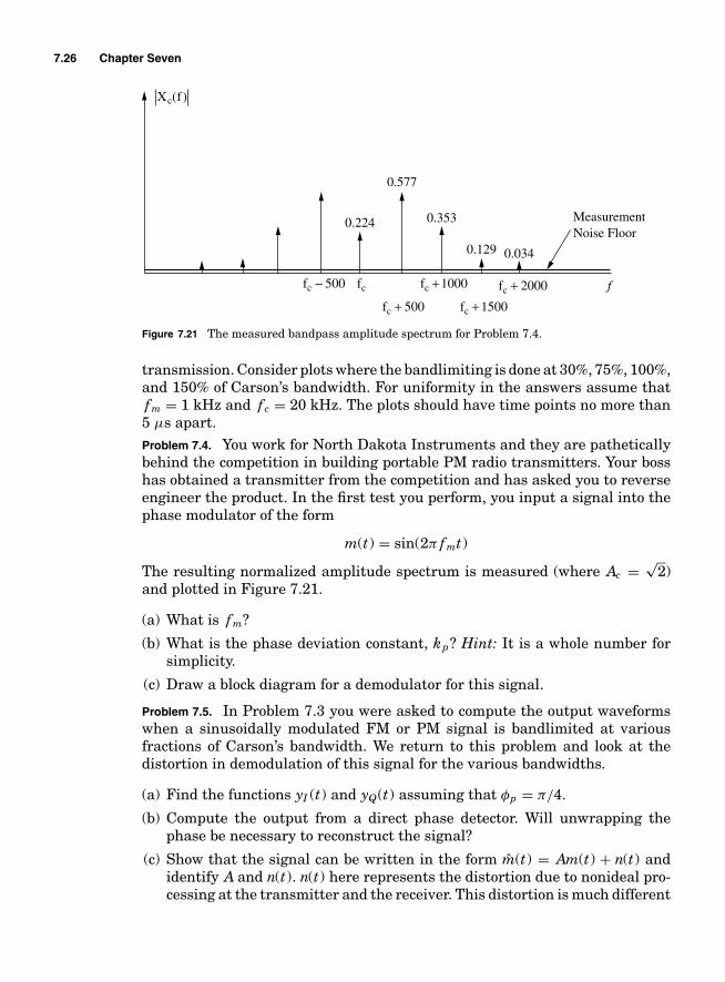
7.26 Chapter Seven
0.224
0.577
0.353
0.129
MeasurementNoise Floor
fc
fc + 500
fc +1000
fc + 1500
0.034
fc + 2000fc − 500
X fc( )
f
Figure 7.21 The measured bandpass amplitude spectrum for Problem 7.4.
transmission. Consider plots where the bandlimiting is done at 30%, 75%, 100%,and 150% of Carson’s bandwidth. For uniformity in the answers assume thatfm = 1 kHz and f c = 20 kHz. The plots should have time points no more than5 µs apart.Problem 7.4. You work for North Dakota Instruments and they are patheticallybehind the competition in building portable PM radio transmitters. Your bosshas obtained a transmitter from the competition and has asked you to reverseengineer the product. In the first test you perform, you input a signal into thephase modulator of the form
m(t) = sin(2π fmt)
The resulting normalized amplitude spectrum is measured (where Ac = √2)
and plotted in Figure 7.21.
(a) What is fm?
(b) What is the phase deviation constant, kp? Hint: It is a whole number forsimplicity.
(c) Draw a block diagram for a demodulator for this signal.
Problem 7.5. In Problem 7.3 you were asked to compute the output waveformswhen a sinusoidally modulated FM or PM signal is bandlimited at variousfractions of Carson’s bandwidth. We return to this problem and look at thedistortion in demodulation of this signal for the various bandwidths.
(a) Find the functions yI (t) and yQ(t) assuming that φp = π/4.
(b) Compute the output from a direct phase detector. Will unwrapping thephase be necessary to reconstruct the signal?
(c) Show that the signal can be written in the form m(t) = Am(t) + n(t) andidentify A and n(t). n(t) here represents the distortion due to nonideal pro-cessing at the transmitter and the receiver. This distortion is much different

Analog Angle Modulation 7.27
than the noise that will be introduced in Chapters 9 and 10 but producessimilar effects.
(d) With
S N R = A2 Pm
Pn
Find BT such that the SNR > 30 dB Hint: n(t) is periodic with the sameperiod as the message signal so Pn can be computed in a simple way.
Problem 7.6. A test tone of frequency fm = 1000 Hz with an amplitude Am = 2volts is to be transmitted using both frequency modulation (FM) and phasemodulation (PM).
(a) Give values of kp and kf to achieve a β = 2. Using Carson’s rule what isthe resulting transmission bandwidth.
(b) Keeping Am, kp, and kf the same as in part (a) and setting fm = 200 Hzcompute the resulting transmission bandwidth for both modulations.
(c) Keeping Am, kp, and kf the same as in part (a) and setting fm = 5000 Hzcompute the resulting transmission bandwidth for both modulations.
(d) What characteristic does FM have that would be an advantage in a practicalsystem?
Problem 7.7. A message signal, m(t), with bandwidth W = 10 kHz, max |m(t)| =Am, and average power Pm is frequency modulated (FM) (the frequency devia-tion constant is kf radians/second/volt) onto a carrier ( f c) with amplitude Ac.
(a) Give the form of the transmitted signal (either in bandpass form or complexbaseband form).
(b) Choose the signal parameters such that the transmitted power is Pxc =25 W in a 1-� system.
(c) Define the deviation ratio, D, for an FM signal and choose the signal para-meters such that D = 4.
(d) With D = 4 give a transmission bandwidth which will contain approxi-mately 98% of the signal power.
Problem 7.8. As a new engineer at Badcomm, you are given the task to reverseengineer a phase modulator made by your competitor.
(a) Given your lab bench contains a signal generator and a spectrum analyzer,describe a test procedure that would completely characterize the phasemodulator.
(b) Given your lab bench contains a signal generator, a bandpass filter withcenter frequency f c and bandwidth 2000 Hz, a power meter, and an I/Qdownconverter describe a test procedure that would completely characterizethe phase modulator.

7.28 Chapter Seven
Problem 7.9. This problem is concerned with frequency modulation (FM) by themessage signal given in Problem 5.1. Assume a carrier frequency of f c =1000 Hz, a radian frequency deviation constant of kf and a carrier amplitudeof Ac.
(a) Give the baseband, xz(t), and bandpass, xc(t), time waveforms.
(b) Using the results of Problem 5.1 what is the peak frequency deviation?
(c) State Carson’s rule for an arbitrary message signal that is angle modulated.Select a value of kf that will achieve a Carson’s rule bandwidth of 600 Hzfor FM with a message signal given in Problem 5.1.
(d) For the value of kf selected in (c) plot the bandpass time waveform, xc(t)and the vector diagram of xz(t).
(e) Use Matlab to compute a measured power spectrum. How do the resultscompare to that predicted by the Carson’s rule approximation?
(f) Give the value of Ac that will produce a 50-W output power in a 1-� system.
Problem 7.10. Repeat Problem 7.9 with the message signal of Problem 5.5 exceptwith a Carson’s rule bandwidth of 20 Hz and a carrier frequency of f c = 40 Hz.
Problem 7.11. This problem is concerned with phase modulation (PM) by the mes-sage signal given in Problem 5.1. Assume a carrier frequency of f c = 1000 Hz,a phase deviation constant of kp and a carrier amplitude of Ac.
(a) Give the baseband, xz(t), and bandpass, xc(t), bandpass time waveforms.
(b) Using the results of Problem 5.1 what is the peak frequency deviation?
(c) State Carson’s rule for an arbitrarily message signal that is angle modu-lated. Select a value of kp that will achieve a Carson’s rule bandwidth of600 Hz for PM with a message signal given in Problem 4.1.
(d) For the value of kp selected in (c) plot the bandpass time waveform, xc(t)and the vector diagram of xz(t).
(e) Use Matlab to compute a measured power spectrum. How do the resultscompare to that predicted by the Carson’s rule approximation?
(f) Give the value of Ac that will produce a 50-W output power in a 1-� system.
Problem 7.12. Repeat Problem 7.11 with the message signal of Problem 5.5 exceptwith a Carson’s rule bandwidth of 20 Hz and a carrier frequency of f c = 40 Hz.
Problem 7.13. Angle modulation with a sinusoidal message signal has the form
xz(t) = Ac exp[ jβ sin(2π fmt)]
The vector diagram of the received signal yz(t) is plotted in Figure 7.22 for0 ≤ t ≤ ( fm)−1.

Analog Angle Modulation 7.29
0
A B
C
0
1
1
−1
−1
y tI ( )
yt
Q()
Figure 7.22 A vector diagram for a sinusoidal angle modulation for Problem 7.13.
(a) What are the approximate values of Ac, β, and φp?
(b) Give the approximate values of time (or times) associated with each labeledpoint (A, B, & C).
Problem 7.14. For m(t) = sin(2π fmt) the received complex envelope is
yz(t) = 5 exp[ j (0.1 cos(2π fmt − π ) + π/5)]
Identify as many parameters of the modulation and channel as possible.
Problem 7.15. The waveform shown in Figure 7.23 is phase modulated on a car-rier with kp = π/3.
(a) Plot the output bandpass waveform for f c = 10 fm. For uniformity in theanswers assume that fm = 1 kHz and f c = 10 kHz. The plots should havetime points no more than 5 µs apart.

7.30 Chapter Seven
1
m(t)
1 fm
…
t
Figure 7.23 Message waveform for Problem 7.15.
(b) This same bandpass waveform can be generated with frequency modula-tion (FM). Specify the message signal and the f k that achieves the samewaveform as plotted in part (a).
Problem 7.16. (UM) In this problem, you will consider the effects of the mes-sage amplitude on angle modulation. Consider a message signal, m(t) = 2 cos(2000πt). Let the deviation constants be kp = 1.5 radians/volt and f k =3000 Hz/V.
(a) Determine the modulation indices: βp for PM and β f for FM.
(b) Determine the engineering transmission bandwidths.
(c) Plot the spectrum of the complex envelopes, considering only those compo-nents that will lie within the transmission bandwidth determined above.Hint: You’ll need to think about what the modulated signal will look like.
(d) If the amplitude of m(t) is decreased by a factor of two, how will your pre-vious answers change?
You can use Matlab to compute the Bessel function evaluated for relevant ordersand relevant arguments (besselj(n,x)).
Problem 7.17. Consider the following complex envelope signal for angle modu-lation with a sinusoidal message xz(t) = exp[ jβ cos(2π fmt)] and compute theFourier series. Recall that sin
(θ + π
2
) = cos(θ). How does the power spectrumof this complex envelope compare to the signal considered in Eq. (7.5)?
Problem 7.18. You are making a radio transmitter with a carrier frequency f cthat uses an angle modulation. The message signal is a sinusoid with Am = 1and the complex envelope of the signal output from your voltage controlledoscillator is
xz(t) = 2 exp[ jβ sin(2π500t)] (7.38)
where β is a constant.

Analog Angle Modulation 7.31
(a) Choose β such that BT = 6000 Hz (use Carson’s rule).
(b) The output spectrum for this transmitted signal will have a line (or impul-sive) spectrum since the baseband signal is periodic. What is the value ofthe output bandpass spectrum impulse at f = f c for the value of β givenin part (a).
(c) What is the message signal and the value of kp if the signal is phase modu-lated (PM)?
(d) What is the message signal and the value of kf if the signal is frequencymodulated (FM)?
(e) For PM if fm is reduced from 500 Hz to 100 Hz choose a value of kp suchthat the output bandwidth is still BT = 6000 Hz according to Carson’s rule.
(f) For FM if fm is reduced from 500 Hz to 100 Hz choose a value of kf suchthat the output bandwidth is still BT = 6000 Hz according to Carson’s rule.
Problem 7.19. Recall that narrowband phase modulation has a very similar formto LC-AM, i.e.,
xc(t) ≈ Ac
√2 cos(2π f ct) − Ackpm(t)
√2 sin(2π f ct) (PM)
xc(t) = Ac
√2 cos(2π f ct) + Acam(t)
√2 cos(2π f ct) (AM)
Because of this similarity one might be tempted to use an envelope detector asa simple demodulator.
(a) Compute the envelope, yA(t), of the received signal.
(b) Consider a simple example with m(t) = cos(2π(100)t) and kp = 0.1. Plot thevector diagram of the true PM signal and the approximate form in Eq. (7.20).
(c) Plot the envelope for the signal in Eq. (7.20).
(d) Could the envelope detector be used for demodulating narrowband PM?
Problem 7.20. For a sinusoidal angle modulated signal
xz(t) = Ac exp[ jβ sin(2π500t)] (7.39)
and a propagation phase rotation of φp.
(a) For φp = 0, how large could β be and not require phase unwrapping?
(b) For φp = π2 , how large could β be and not require phase unwrapping?
(c) For φp = − 7π8 , how large could β be and not require phase unwrapping?
Problem 7.21. What condition must hold for the message signal, m(t), and themodulation constants, kp and kf , such that the signals in Eq. (7.36) are guar-anteed to be of the form of a LC-AM signal.

7.32 Chapter Seven
Problem 7.22. In a digital receiver samples of the complex envelope, yz(kTs),are often processed to demodulate a message signal. Here Ts is the sampleperiod and k enumerates the sample number. Assume the received signal isFM modulated, i.e.,
yz(t) = Ac exp(
j kf
∫ t
−∞m(λ)dλ + φp
)(7.40)
(a) Show that if the sampling frequency is high enough that
q(k) = yz(kTs)y∗z ((k − 1)Ts) ≈ A2
c exp( j Km(t)) (7.41)
(b) Postulate how small Ts must be such that the result in (a) holds with a goodaccuracy.
(c) Identify the value of K .
(d) Using the idea in (a) as a basis for an FM demodulator, show a block diagramof the whole FM demodulator.
Problem 7.23. You have been given the received complex envelope, yz(t) = yI (t)+j yQ(t), of a periodic message signal transmitted via phase modulation (PM) asshown in Figure 7.24. The message signal has an average value of 0 so that itwill pass through a DC block unchanged and max |m(t)| = 1.
(a) Give the form of the received complex envelope for PM, yz(t) as a functionof the phase deviation constant kp, Ac, m(t), and φp.
(b) Find yA(t) and use that to find Ac.
t
yQ(t)
yI(t)
t
1 2 3 4 5 6
1
−1
−1
2
……
… …
1 2 3 4 5 6
Figure 7.24 The received complex envelope of a PM signal.

Analog Angle Modulation 7.33
15 kHz−15 kHz
M( f )
Figure 7.25 An example spectrum for audio broadcast.
(c) Find received phase yP (t) from the data in Figure 7.24. Hint: I made it easyenough to do without calculators or Matlab.
(d) Pass yP (t) through a PM demodulator and use the result to find a possiblemessage signal and a value of kp. Will phase unwrapping be necessary?
(e) Find the transmitted power, Pxz .
Problem 7.24. High fidelity audio broadcast typically tries to maintain a 15 kHzof bandwidth in transmitting to listener. An example audio spectrum is givenin Figure 7.25.
(a) In the days before stereo became a reality FM broadcasts frequency modu-lated a message signal of the form seen in Figure 7.25 onto a carrier. TheFCC set f p ≤ 75 kHz. Using Carson’s rule determine the D that wouldachieve a 98% power bandwidth of 180 kHz.
(b) After these allocations were set in concrete by the FCC stereo audio becamea reality. After long discussions by the communication engineers of the dayit was decided that stereo FM was possible if the input message signalto the FM modulator had the spectrum seen in Figure 7.26. Essentiallythe signal resulting from the sum of the left and right channels, mS (t) =mL(t) + mR(t) is combined with an DSB-AM modulated signal ( f c = 38 kHz)of the difference of the left and the right channels, mD(t) = mL(t) − mR(t).This way of combining the left and right channel was considered a nice
19 kHz
15 kHz
Pilot Tone Pilot Tone
M( f )
23 kHz38 kHz−38 kHz f
Figure 7.26 Stereo FM message signal.
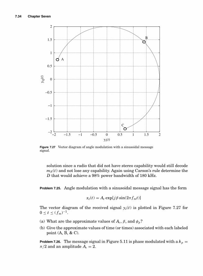
7.34 Chapter Seven
A
B
C
−2 −1.5 −1 −0.5 0yl(t)
y Q(t
)
0.5 1 1.5 2−2
−1.5
−1
−0.5
0
0.5
1
1.5
2
Figure 7.27 Vector diagram of angle modulation with a sinusoidal messagesignal.
solution since a radio that did not have stereo capability would still decodemS (t) and not lose any capability. Again using Carson’s rule determine theD that would achieve a 98% power bandwidth of 180 kHz.
Problem 7.25. Angle modulation with a sinusoidal message signal has the form
xz(t) = Ac exp[ jβ sin(2π fmt)]
The vector diagram of the received signal yz(t) is plotted in Figure 7.27 for0 ≤ t ≤ ( fm)−1.
(a) What are the approximate values of Ac, β, and φp?
(b) Give the approximate values of time (or times) associated with each labeledpoint (A, B, & C).
Problem 7.26. The message signal in Figure 5.11 is phase modulated with a kp =π/2 and an amplitude Ac = 2.

Analog Angle Modulation 7.35
(a) What is the form for xz(t).
(b) What is the transmitted power?
(c) Plot the instantaneous frequency deviation, fd (t).
(d) Plot a vector diagram of xz(t). Clearly label the points corresponding tot = 0, T /4, T /2, 3T /4, T .
(e) Is xz(t) a periodic signal? If so what is the fundamental frequency?
(f) Using Carson’s rule estimate the 98% bandpass bandwidth of this phasemodulated signal.
(g) The spectrum of the bandpass signal will be impulsive (discrete frequen-cies). What will be the value of the impulse at f = f c.
Problem 7.27. If m(t) is periodic with period T
(a) What is the largest possible period of a phase modulated signal with phasedeviation constant kp?
(b) Is it possible for the period of xz(t) to be less than T ? If yes, give an example.
(c) State a condition on m(t) such that Fourier series coefficient for DC,
z0 =∫ T
0xz(t)dt (7.42)
is real valued.
Problem 7.28. If m(t) is periodic with period T and the integral of m(t) is
mi(t) =∫ t
−∞m(λ)dλ (7.43)
(a) State a condition on m(t) such that mi(t) is periodic with the same period.
(b) Can mi(t) be aperiodic but xz(t) = exp[ j mi(t)] be periodic? Give an exampleif the statement is true.
Problem 7.29. A periodic received signal, rz(t), from an analog modulation isgiven in Figure 7.28.
r tI( ) r tQ( )
−1 −1
1
T T… … … …
Figure 7.28 A received complex envelope.

7.36 Chapter Seven
(a) Assume the transmitted signal is given as xz(t), how have we modeled theform for rz(t) in terms of xz(t) for this class?
(b) Given rz(t) in Figure 7.28, is it possible for the transmitted signal to be aPM signal? Why?
Problem 7.30. For m(t) = cos(200πt) a received complex envelope in the absenceof any noise is
yz(t) = 5 exp[ j (0.8 sin(200πt) + π/5)]
(a) With what modulation has the analog message been transmitted?
(b) Identify as many parameters of the modulation and the channel aspossible.
(c) You have been tasked to build a lowpass filter for the signals yI (t) andyQ(t) such that you pass about 98% of the power of the signals. With whatbandwidth should the lowpass filters be designed?
Problem 7.31. The message signal detailed in Problem 5.5 is used in a phasemodulation. Assume the amplitude is Ac and that kp = 3.
(a) Choose Ac such that Pxz = 16.
(b) With the Ac as specified in a) plot xI (t) and xQ(t).
(c) Find D.
(d) Use D and Carson’s rule to estimate BT . What is EB ?
(e) Assume φp = π/4 and plot yI (t), yQ(t), and yp(t).
Problem 7.32. (JG) If the waveform in Figure 7.29 is input into an anglemodulator,
0 0.5 1 1.5 2 2.5 3 3.5 4 4.5 5
0
0.5
−0.5
1
−1
1.5
−1.5
2
−2
m(t
)
t
Figure 7.29 A message signal.

Analog Angle Modulation 7.37
(a) Derive an expression for the time domain bandpass waveform if PM is usedwith kp = π and Ac = 1/
√2. Plot the PM signal for f c = 4.
(b) Derive an expression for the time domain bandpass waveform if FM is usedwith kf = 2π and Ac = 1/
√2. Plot the FM signal for f c = 4.
Problem 7.33. An often used pulse in radar systems has a complex envelope of
xz(t) ={
Ac exp[
j 2πg0t2] 0 ≤ t ≤ Tp
0 elsewhere(7.44)
(a) Is this an angle modulated signal? Justify your answer.
(b) Plot the bandpass signal, xc(t) for f c = 10 Hz and g0 = 100 Hz/s, Ac = 1,and Tp = 1.
(c) Find the instantaneous frequency deviation, fd (t), and the peak frequencydeviation, f p, for this signal.
(d) Plot Gxz(f ) and estimate B98 when g0 = 100 Hz/s and Tp = 1.
(e) Show that Carson’s rule of thumb does not hold for this signal and identifythe characteristic of this radar signal that is different than a typical anglemodulated message signal that causes this well respected rule of thumb notto hold.
7.6 Example Solutions
Problem 7.7.
(a) The complex baseband signal for FM is given as
xz(t) = Ac exp[
j kf
∫ t
−∞m(λ)dλ
](7.45)
The bandpass signal is given as
xc(t) = Ac
√2 cos(
2π f ct + kf
∫ t
−∞m(λ)dλ
)(7.46)
(b) Since Pxc = 25 = A2c it is straightforward to see that Ac = 5
(c) The definition of the deviation ratio is
D = f k max |m(t)|W
(7.47)
Rearranging gives
max |m(t)| = 40, 000f k
(7.48)
(d) Using Carson’s rule gives BT = 2(D +1)W = 2×5×10, 000 = 100,000 Hz.

7.38 Chapter Seven
Problem 7.18.
(a) Carson’s rule gives
BT = 2(β + 1) fm (7.49)
6000 = 2(β + 1)500 (7.50)
Solving gives β = 5.
(b) Using the results in Eq. (6.7) gives
xz(t) =∞∑
n=−∞Ac Jn(β) · e( j 2π fmnt) (7.51)
and consequently
Xz(f ) =∞∑
n=−∞Ac Jn(β)δ( f − nfm) (7.52)
Note Ac = 2 and β = 5 and recall the relationship between the basebandand bandpass spectrum is
Xc(f ) = 1√2
Xz( f − f c) + 1√2
X ∗z (− f − f c) (7.53)
=∞∑
n=−∞
Ac Jn(β)√2
δ( f − nfm − f c) +∞∑
n=−∞
Ac Jn(β)√2
δ( f + nfm + f c)
(7.54)
so consequently the value of the spectral impulse at f c is 2J0(5)√2
= −0.3678
(c) Recall
kp · m(t) = 5 sin(2π fmt) (7.55)
and since Am = 1 we have kp = 5 and m(t) = sin(1000πt).
(d) Recall
kf
∫ t
−∞m(λ)dλ = 5 sin(2π fmt) (7.56)
consequently
kf m(t) = 5ddt
sin(2π fmt) = 5(2π fm) cos(2π fmt) (7.57)
and since Am = 1 we have kf = 5(2π fm) = 5000π rad/s/V and m(t) =cos(1000πt).

Analog Angle Modulation 7.39
(e) Carson’s rule gives
BT = 2(β + 1) fm (7.58)
6000 = 2(β + 1)100 (7.59)
Solving gives β = kp = 29.
(f) Carson’s rule again gives β = 29 and kf = β(2π fm) = 5800π rad/s/V.Parts (e) and (f) show one of the interesting differences between FM andPM. A characteristic of FM is that once the frequncy deviation is chosenthe transmission bandwidth remains relatively constant regardless of thesignal bandwidth. PM on the otherhand has the transmission bandwidthvarying in direct proportion to the message signal bandwidth for a fixedphase deviation constant. This is one reason why FM is preferred in practiceto PM.
7.7 Miniprojects
Goal: To give exposure
■ to a small scope engineering design problem in communications.■ to the dynamics of working with a team.■ to the importance of engineering communication skills (in this case oral pre-
sentations).
Presentation: The forum will be similar to a design review at a company(only much shorter). The presentation will be of 5 minutes in length with anoverview of the given problem and solution. The presentation will be followedby questions from the audience (your classmates and the professor). Each teammember should be prepared to make the presentation on the due date.
7.7.1 Project 1
Project Goals: Undergraduate communication courses often only look at ide-alized problems. For example, one thing that is ignored in a course is that fre-quency sources at the transmitter and receiver cannot be made to have exactlythe same value. This miniproject will investigate the effects of this frequencyoffset on one phase demodulation algorithm.
When a frequency offset exists the complex envelope of the received signalwill be rotating due to this frequency offset, i.e.,
yz(t) = xz(t) exp[ j (φp + 2π f ot)] (7.60)
where f o is the existing frequency offset. Get the Matlab file angmodex1.m andangmodex3.m from the class web page. In these files a PM transmitter (for asinusoid message signal) and receiver is implemented. If the carrier frequencyoffset is set to 10 Hz (in the Matlab code deltaf = 10) the demodulator

7.40 Chapter Seven
implemented in the m-file still works pretty well with this frequency offset.Explain why. Note, at higher frequency offsets (e.g., 100 Hz) the performancesuffers noticeable distortion. Extra credit will be given if you can figure out amethod to eliminate this distortion.
7.7.2 Project 2
Project Goals: Use your knowledge of communication theory to decode anunknown analog modulated signal.
You have been hired by the National Security Agency of the US Federalgovernment as an engineer. The first job you have been given by your new bossis to decode a radio message signal between two members of a South Albumandrug cartel. This signal was intercepted by a spy satellite and the data has beenprocessed and forwarded on to you for decoding.
The technical details are
■ The sampled data file contains about 1 second worth of data at a 44,100-Hzsampling rate. (Precisely 44,864 samples). This data is available at the classweb site in the file entitled Intercept.mat.
■ The radio signal is analog modulated. The type of analog modulation is un-clear. Human intelligence sources have indicated that the modulation usedis either DSB-AM, LC-AM, SSB-AM, or PM.
■ The carrier frequency is unknown. Obviously since the data is provided toyou with a sample rate of 44,100 Hz the carrier frequency must be between0 and 22,050 Hz.
■ The channel includes an unknown delay that produces an unknown phaseshift, ϕp.
Your job is to decode the signal. It should be obvious when you are correct asyou can play the demodulated output as a sound. The solution should include
■ a discussion of the methodology that led you to identifying the modulation.■ a discussion of the methodology that led you to identifying the carrier fre-
quency.■ a discussion of the demodulator architecture and the method used to estimate
the phase shift or to operate in the presence of an unknown phase shift.■ submission of Matlab code for the demodulator.
Chapter
8More Topics in Analog
Communications
This chapter covers two topics which are important for both amplitude and an-gle modulation methods of analog communications: the phase-locked loop andthe multiplexing of message signals. In fact, almost all modern communicationssystems, analog or digital, contain a phase-locked loop and contain some formof multiplexing.
8.1 Phase-Locked Loops
8.1.1 General Concepts
The phase-locked loop (PLL) is a commonly used component in communica-tion systems. It can be used for tracking the phase and frequency of signals,demodulating angle modulated signals, and frequency source synthesis. ThePLL is a tracking system that uses feedback. We have seen one example sofar in the Costas loop for synchronous demodulation of DSB-AM. This sectionwill investigate the use of the PLL for FM and PM demodulation (feedbackdemodulation) but the general characteristics are valid for any application ofthe PLL. The input complex signal into a PLL has amplitude variation A(t), aphase variation, θ (t), and a nuisance phase variation, d (t). The goal of a PLL,in most cases, is to track and/or estimate the value of θ(t).
The typical PLL, seen in Figure 8.1, has three components: the phase detector,the loop filter, and the voltage controlled oscillator (VCO). Recall the VCO hasthe characteristics shown in Figure 8.2. The VCO has a quiescent frequency off c and a gain of kf = 2π fd radians/s/volt.
EXAMPLE 8.1For demodulation of PM we have A(t) = Ac, θ(t) = kpm(t) + φp , and d (t) = 0.
8.1
Copyright © 2007 by The McGraw-Hill Companies. Click here for terms of use.

8.2 Chapter Eight
PhaseDetector
VCO
LoopFilter
e td ( )
y td ( )
A t j d t t( )exp ( ) ( )+( )[ ]θ
j texp ( )[ ]θ
Figure 8.1 Phase-locked loop block diagram.
EXAMPLE 8.2For the Costas loop used as a synchronous demodulator for DSB-AM we have A(t) =Ac|m(t)|, θ (t) = φp , and d (t) = (1 − m(t)) π
2 .
The phase detector simply measures the phase difference between the inputsignal and the locally generated reference. Denoting the input signal to the PLLas yz(t) the phase detector is a nonlinear function denoted ed (t) = g(yz(t), θ (t)),which is usually designed to be proportional to the phase error ϕ(t) = θ (t) − θ (t).
EXAMPLE 8.3The most common phase detector for an unmodulated sinusoidal input signal (A(t) = Acand d (t) = 0) is the quadrature multiplier and the analytical model is seen in Figure 8.3.This phase detector is given as
g(yz(t), θ (t)) = Ackm�[yz(t) exp[− j θ (t)]]
VCOIn Out
Kv
Bandpass
VCOIn Out
Kv
Baseband
y td ( ) 2 cos 2π fct + k f yd λ( )dλ−∞
t
∫⎛
⎝⎜⎞
⎠⎟
exp jkf yd λ( )dλ⎛
⎝⎜⎞
⎠⎟y td ( )
−∞
t
∫
Figure 8.2 The bandpass and baseband block diagrams for a VCO.

More Topics in Analog Communications 8.3
e td( )A j tc exp θ( )[ ] km
( )*
Im •[ ]
exp j θ t( )⎡⎣ ⎤⎦
Figure 8.3 The quadrature multiplier phase detector blockdiagram.
where km is the multiplier gain. The phase detector output can be expressed in termsof the phase error as
ed (t) = Ackm sin(θ(t) − θ(t)) = Ackm sin(ϕ(t))
The signal ed (t) is a function of the phase error and it can be used as a feedback signalin a closed loop tracking system.
EXAMPLE 8.4Note, Figure 6.9 shows another type of a phase detector which is useful for phase trackingwith DSB-AM signals (A(t) �= Ac and d (t) �= 0). The phase detector is given as
g(yz(t), θ(t)) = km�[(yz(t) exp[− j θ (t)])2]= 2km�[yz(t) exp[− j θ (t)]][yz(t) exp[− j θ (t)]] (8.1)
Expressing the phase detector output in terms of the phase error gives
ed (t) = km A2c m2(t) sin(2ϕ(t))
The loop filter is a linear filter and its design is often critical in getting thedesired performance out of a PLL. For this development the loop filter is rep-resented with F (s). Two common types of loops are the first and second orderPLL. The first-order PLL loop filter has a transfer function given as
F (s) = 1
and the second-order PLL loop filter is given as
F (s) = s + as + b
It should be noted that the most common type of second order loop is one witha perfect integrator (b = 0). The second-order PLL loop filter is more commonlyused in practice because it can both track a phase and a frequency offset.

8.4 Chapter Eight
F(s)
yd(t)
+
−θ( )t kd
e td( )
kfs
θ t( )
Σ
Figure 8.4 The linear model ofthe phase-locked loop.
8.1.2 PLL Linear Model
The linear analysis of the PLL is valid when the loop is closely tracking theinput signal (ϕ(t) ≈ 0). Close tracking implies that ϕ(t) is small and that thephase detector can be linearized around ϕ(t) = 0 so that
g(yz(t), θ (t)) ≈ kd ϕ(t)
where kd is denoted the phase detector gain. This results in a linear model forthe PLL that is shown in Figure 8.4. Note, since the phase of the VCO outputis proportional to the integral of the input signal the VCO can be modeled by atransfer function with a Laplace transform of kf/s where kf is the gain of theVCO.
EXAMPLE 8.5The quadrature multiplier has ed (t) = Ackm sin(ϕ(t)) so that the linear approximationhas kd = Ackm and sin(ϕ(t)) ≈ ϕ(t).
8.2 PLL–Based Angle Demodulation
8.2.1 General Concepts
Demodulation of angle modulations with a PLL is actually quite simple con-ceptually. This section will concentrate on demodulation of FM signals and thedifferences for PM will be pointed out when appropriate. Recall a received FMsignal has the form
yz(t) = Ac exp[
j kf
∫ t
−∞m(λ)dλ + j φp
](8.2)
Figure 8.5 shows a block diagram of an FM system with a feedback demodulator.A VCO is used to produce the FM signal and the proposed receiver consists ofa two input, one output black box and a VCO identical to the one used formodulation. After a transient period if θ(t) = θ(t) then we know m(t) = m(t).The job of the black box in the diagram is to measure the phase difference

More Topics in Analog Communications 8.5
VCOm(t)In Out
Transmitter
VCOInOut
Receiver
Black Box
Channel
kf
kf
exp j pφ[ ] m t( )
Figure 8.5 The conceptual diagram for FM demodulation.
ϕ(t) = θ (t) − θ (t) and update m(t) in such a way as to drive ϕ(t) to zero. Notethat if
ϕ(t) = θ (t) − θ(t) < 0 ⇒∫ t
−∞m(λ)dλ <
∫ t
−∞m(λ)dλ
ϕ(t) = θ (t) − θ(t) > 0 ⇒∫ t
−∞m(λ)dλ >
∫ t
−∞m(λ)dλ (8.3)
Equation (8.3) indicates that ϕ(t) can be driven to zero if m(t) is updated inproportion to ϕ(t). Thus the black box in Figure 8.5 is composed of the othertwo elements of the PLL: the phase detector and the loop filter.
Since the FM signal has a constant amplitude the quadrature multiplier (seeFigure 8.3) can be used as the phase detector. Consequently, the overall blockdiagram is seen in Figure 8.6 and the equation defining the operation is
m(t) = f (t) ∗ kd sin(
kf
∫ t
−∞(m(λ) − m(λ))dλ + φp
)(8.4)
where kd = Ackm is the quadrature multiplier phase detector gain. It is im-portant to note that the phase detector gain is a function of the received signalamplitude. While this amplitude is treated as a known constant in these notesin practical systems accounting for this amplitude is an important function ina FM demodulator based on a PLL.
F s( )
( )*
y tz( )e td( )
VCOkf
km
m t( )
Im •[ ]
Figure 8.6 The block diagram of a PLL for FM demodulation.

8.6 Chapter Eight
Equation (8.4) is a nonlinear integral equation that can be solved but onlywith mathematical tools that undergraduate engineering students typicallyhave not been exposed to. Consequently, this presentation examines approxi-mations that simplify the mathematical description of a PLL. This simplifieddescription enables the use of undergraduate engineering tools to be applied tothe problem of analyzing the performance of a PLL. These approximations willgive some design insights and provide a rough performance characterization.
8.2.2 PLL Linear Model
The linear analysis of the PLL is valid when the loop is closely tracking theinput signal. Close tracking implies that ϕ(t) is small and for the quadraturemultiplier phase detector
ed (t) = Ackm sin(ϕ(t)) ≈ Ackmϕ(t) = kd ϕ(t)
This results in a linear model for a PLL used in FM demodulation that is shownin Figure 8.7. Rearranging and defining k = kf kd gives the block diagramshown in Figure 8.8. It is quite obvious from Figure 8.8 that the linear model forthe PLL reduces to a simple linear feedback control system commonly studiedin an undergraduate program. Taking Laplace transforms yield
(M(s) − M(s))kF (s)
s= M(s)
Solving for the transfer function gives
HL(s) = M(s)M(s)
= kF (s)s + kF (s)
(8.5)
Often the error between the demodulated output and the message signal is ofinterest. Defining e(t) = m(t) − yd (t) and using identical techniques a transferfunction for the error is given as
HE (s) = E(s)M(s)
= ss + kF (s)
+
−m t( ) F s( )kf kd
s Σ
m t( )kfs
Figure 8.7 The PLL linear model for FM demodula-tion.

More Topics in Analog Communications 8.7
+
−
ks F s( )m t( )
m t( )
ΣFigure 8.8 The PLL linear modelrearranged to have a classic feed-back control systems structure.
Frequency Response
The frequency response of the loop is of interest. The frequency response isgiven as
H (f ) = H (s)|s= j 2π f
The loop and error transfer functions are plotted Figure 8.9 for a first-order loopwith k = 1000. Consequently, when the linear model is valid the PLL appearsmuch like a lowpass filter to the message signal. For example, for the caseconsidered in Figure 8.9 (k = 1000) the 3 dB-loop bandwidth is about 100 Hz.Consequently, design of PLLs for FM demodulation must carefully consider thebandwidth of the message signal in choosing the bandwidth of the loop.
Acquisition
Let’s consider the transient response produced by a first-order loop (F (s) = 1)to a sinusoidal input signal, m(t) = sin(2π fmt). The Laplace transform of thissignal is
M(s) = 2π fm
s2 + (2π fm)2 (8.6)
−120
−100
−80
−60
−40
−20
0
20
Tra
nsfe
r Fu
nctio
n, d
B
1 10 100 1000 104 105
HE(f)
Frequency, f, Hz
HL(f)
Figure 8.9 The frequency response of a first-order PLL used for FM demodula-tion. k = 1000

8.8 Chapter Eight
−1.5
−1
−0.5
0
0.5
1
1.5
2
0 0.25 0.5 0.75 1 1.25t∗fm
m(t)
f = 10 Hz
f = 1000 Hz
1.5 1.75 2
Figure 8.10 The time response of the linear model of a PLL for FM demodulation.
Using Eq. (8.6) in Eq. (8.5) produces a loop output Laplace transform of
M(s) = 2π fm
s2 + (2π fm)2
ks + k
Inverse transforming this signal gives
m(t) = k(2π fm)k2 + (2π fm)2 e−kt + k√
k2 + (2π fm)2sin[2π fmt + tan−1
(2π fm
k
)]
Figure 8.10 shows a plot of the time response for k = 1000 and fm = 10 andfm = 1000. Note that if the signal is inside the passband of the loop, the loopquickly locks onto the signal and tracks it very closely. If the signal is outside theloop bandwidth the signal is not tracked and the FM demodulation performanceis poor.
8.3 Multiplexing Analog Signals
Definition 8.1 Multiplexing for analog message signals is the common transmission ofmultiple message signals using a single communications resource.
The common resource is typically spectrum (e.g., broadcast radio), expensiveelectronic equipment (e.g., satellites), or both (e.g., analog cellular telephony).For this discussion we will denote the ith message signal as mi(t) and K as

More Topics in Analog Communications 8.9
Multiplexer Resource De-multiplexer
m t1( )
m t2( )
m tK( )
x tc( ) y tc( )
m1 t( )
m2 t( )
mK t( )
Figure 8.11 The multiplexing concept.
the number of users of the resource. Consequently, the idea of multiplexing isshown in Figure 8.11. As a measure of how efficiently we are using the resourcewe define the multiplexing efficiency as
EM =∑K
i=1 Wi
BT(8.7)
where Wi is the ith message bandwidth and BT is the transmission bandwidthof the composite signal. Note, the best multiplexing efficiency without signifi-cant distortion for analog communications is unity. For analog signals there aretwo basic types of multiplexing techniques: (1) quadrature carrier multiplexingand (2) frequency division multiplexing.
EXAMPLE 8.6For those homes that subscribe to cable television services a single cable enters the homewith an electronic signal. Typically greater than 100 channels are supported with thatone cable.
8.3.1 Quadrature Carrier Multiplexing
Quadrature carrier multiplexing (QCM) uses the two degrees of freedom in abandpass signal to transmit two message signals on the same carrier. This typeof multiplexing is achieved by setting xI (t) = Acm1(t) and xQ(t) = Acm2(t). Theblock diagram is shown in Figure 8.12. The efficiency of QCM is
EM = W1 + W2
2 max W1, W2(8.8)
Note, if W1 = W2 then EM = 1 which is the best that can be accomplishedin analog communications. The advantage of QCM is that it is a very efficientmethod of multiplexing message signals. The disadvantage is that the applica-bility is limited to only two message signals and that coherent demodulationmust be used (typically with a transmitted reference carrier which will reducethe bandwidth efficiency somewhat).

8.10 Chapter Eight
I/QUp-converter
ResourceI/Q
Down-converter
m t1( )
x tc( ) y tc( )
m1 t( )
m2 t( )m t2( )
Figure 8.12 Quadrature carrier multiplexing.
8.3.2 Frequency Division Multiplexing
Frequency division multiplexing (FDM) assigns each user a different carrierfrequency for transmission. Typically the carrier frequencies for each user arechosen so that the transmissions do not overlap in frequency. Figure 8.13 showsa typical energy spectrum for a FDM system. Typically each user in the systemis modulated with an analog modulation and has a bandwidth of Bi. This mod-ulation is then separated from its spectral neighbor by a guard band. The sizeof this guard band and the modulation type limits the spectral efficiency. Themultiplexing for FDM is accomplished by simply summing together appropri-ately modulated bandpass waveforms as shown in Figure 8.14. Demultiplexingfor FDM, seen in Figure 8.15, simply corresponds to bandpass filtering to iso-late each user followed by a standard I/Q demodulator. Note, the guard bandsbetween users are usually chosen to be compatible with the bandpass filteringoperation (i.e., the guard band is made large enough to ensure each user canbe adequately separated at the demultiplexer).
EXAMPLE 8.7Broadcast communications in the United States use the resource of free space radio wavepropagation. The multiplexing is typically implemented with a combination of frequency
…
BT
User 1 User 2 User KUser 3
Gxc( f )
B1 B2 B3 BK
fc(K) ffc
(3)fc(2)fc
(1)
Figure 8.13 A typical energy spectrum for a frequency division multiplexed signal.

More Topics in Analog Communications 8.11
I/QUp-converter
I/QUp-converter
I/QUp-converter
fc(1)
xc(1)(t)
xc(2)(t)
fc(2)
fc(K)
xc(K)(t)
xz(K)(t)
Γm(K)(•)
Γm(2)(•)
mK(t)
m2(t)
m1(t)
xz(2)(t)
xz(1)(t)
ResourceΣ xc(t)
Γm(1)(•)
…
Figure 8.14 A FDM multiplexing system.
multiplexing and location multiplexing (stations far enough away from each other canuse the same transmission frequency). AM radio broadcast in the United States has beenassigned the spectrum of 535–1605 kHz, BT = 1070 kHz. There are 107 FDM channelsspaced about 10 kHz apart ( f (i)
c = 540 + 10i kHz). Each AM station provides an audio
Resource
I/Q Down-converter
BPF
fc(K)
fc(K)
BPF
fc(2)
yz(K)(t)
yz(2)(t)
yz(1)(t)
yc(K)(t)
yc(2)(t)
yc(1)(t)
Γd(K)(•)
Γd(2)(•)
Γd(1)(•)
mK(t)
m2(t)
m1(t)
yc(t)
BPF
fc(1)
fc(1)
fc(2)
I/Q Down-converter
I/Q Down-converter
…
ˆ
ˆ
ˆ
Figure 8.15 A FDM demultiplexing system.

8.12 Chapter Eight
ResourceMultiplexer
Multiplexer
Multiplexer
…
xc(1)(t)
xc (t)xc(2)(t)
xc(K2)(t)
mK1
(K2)(t)
m2(K2)(t)
m1(K2)(t)
mK1
(1)(t)
m2(1)(t)
m1(1)(t)
Figure 8.16 A two-level multiplexing scheme.
signal of about 4 kHz bandwidth (Wi = 4 kHz). The efficiency of AM broadcast is thengiven as
EM = 107 × 41070
= 40%
Note, 20% of the loss in efficiency is due to guard bands and 40% of the loss is due tousing spectrally inefficient LC-AM as the modulation.
There can be several levels of multiplexing that are implemented for a givensystem. The first level often groups related messages together and the subse-quent levels multiplex several groups of messages together. The block diagramfor a system using two levels of multiplexing is shown in Figure 8.16.
EXAMPLE 8.8An example of multilevel multiplexing is seen in broadcast communications in theFM band in the United States. Each FM station in the United States typically broad-casts three message signals. Two are audio channels: the left channel, mL(t) and theright channel, mR(t) for stereo broadcast, and one is an auxiliary channel, mA(t) (e.g.,Musak, or Radio Data Services). These three message signals are multiplexing onto one

More Topics in Analog Communications 8.13
composite message signal which is FM modulated and transmitted. For discussion pur-poses the bandwidth of these message signals can be assumed to be Wi = 15 kHz. Thefirst level of multiplexing FDM with m1(t) = mL(t) + mR(t), m2(t) = mL(t) − mR(t),and m3(t) = mA(t), �
(1)m = �
(2)m = �
(3)m = DSB-AM, and f (1)
c = 0, f (2)c = 38 kHz, and
f (3)c = 76 kHz.
8.4 Conclusions
This chapter considered two ideas that have found utility in analog communi-cations; phase locked loops and multiplexing. Phase-locked loops are used in avariety of applications in analog communications. Examples include phase ref-erence estimation and tracking in DSB-AM demodulation and in demodulationof angle modulations. This chapter gave an introductory overview and showedhow tools from feedback control are useful in gaining an understanding of theoperation of phase-locked loops. Multiplexing is an important aspect of commu-nications. Multiplexing allows multiple information sources to be transmittedon a common resource. The common forms of multiplexing for analog commu-nications include quadrature carrier multiplexing and frequency multiplexing.Again the trade-offs between spectral efficiency and complexity were evidentin multiplexing techniques.
8.5 Homework Problems
Problem 8.1. Your boss at Enginola has assigned you to be the systems engineerin charge of an FM demodulator. Unfortunately, this design must be done in oneday. The demodulator is required to be a PLL-based system and since you arepressed for time, you will use the linear approximation for the loop. Figure 8.17is the model for your system.
The transfer function, HL(f ), from the input (m(t)) to the output (m(t)) hasthe form
HL(s) = 2ζωns + ω2n
s2 + 2ζωns + ω2n
PhaseDetector
Loop Filter
VCO
m t( )
φp
θ t( ) k s as
1 +( )m t( ) Σ
k f m λ( )dλ−∞
t
∫
k f m λ( )dλ−∞
t
∫
Figure 8.17 Block diagram of a PLL demodulator for FM.

8.14 Chapter Eight
(a) Select values of kf , k1, and a such that ζ = 1.00 and |HL(12 kHz)| > 0.707(i.e., the 3-dB bandwidth is 12 kHz). Note, while this problem can be com-pleted with pencil and paper, a proficiency with a computer would be useful.
(b) If the input signal is m(t) = sin(2π(10 kHz)t)U (t) where U (t) is the unitstep function, calculate the output response to this signal and plot theresponse.
Problem 8.2. As a communication engineer you need to transmit eight voice sig-nals (W = 4 kHz) across a common communication resource at a carrier fre-quency of 1 GHz. For hardware reasons you need to maintain a 1 kHz guardband between frequency multiplexed transmissions.
(a) If you use DSB-AM and FDM, what is the total used bandwidth, BT , andthe multiplexing efficiency, EM?
(b) If you use SSB-AM and FDM what is the total used bandwidth and themultiplexing efficiency, EM?
(c) If a two-stage multiplexing scheme is employed such that two voice sig-nals are grouped together with QCM and the resulting four signals aremultiplexed using FDM, what is the total bandwidth and the multiplexingefficiency, EM?
Problem 8.3. In the text the example of a first-order loop was considered for FMdemodulation. k = 1000 gave a design of a loop with a bandwidth of about100 Hz.
(a) Redesign the loop gain, k, to give a 3-dB bandwidth of 5 kHz.
(b) Note that the loop gain is a function of the signal amplitude, Ac. Keepingthe remainder of the loop the same and if the signal amplitude is cut in halfwhat will be the loop 3 dB bandwidth?
(c) Keeping the remainder of the loop the same and if the signal amplitude isdoubled what will be the loop 3 dB bandwidth?
(d) Postulate how PLL-based FM demodulators might deal with amplitudevariations in the received signal.
Problem 8.4. High fidelity audio broadcast typically tries to maintain a 15 kHz ofbandwidth in transmitting to listener. An example audio spectrum is given inFigure 8.18. In the days before stereo became a reality FM broadcasts frequencymodulated a message signal of the form seen in Figure 8.18 onto a carrier. Thismessage signal had a bandwidth of 15 kHz.
After FM had been around a while stereo audio became a reality and a finan-cially desirable service to provide. After long discussions by the communicationengineers of the day it was decided that stereo FM was possible if the inputmessage signal to the FM modulator had the spectrum seen in Figure 8.19.Essentially the signal resulting from the sum of the left and right channels,
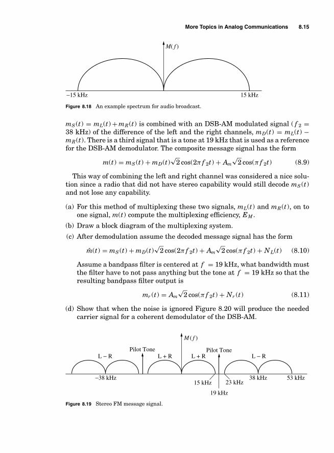
More Topics in Analog Communications 8.15
−15 kHz 15 kHz
M( f )
Figure 8.18 An example spectrum for audio broadcast.
mS (t) = mL(t) + mR(t) is combined with an DSB-AM modulated signal ( f 2 =38 kHz) of the difference of the left and the right channels, mD(t) = mL(t) −mR(t). There is a third signal that is a tone at 19 kHz that is used as a referencefor the DSB-AM demodulator. The composite message signal has the form
m(t) = mS (t) + mD(t)√
2 cos(2π f 2t) + Am
√2 cos(π f 2t) (8.9)
This way of combining the left and right channel was considered a nice solu-tion since a radio that did not have stereo capability would still decode mS (t)and not lose any capability.
(a) For this method of multiplexing these two signals, mL(t) and mR(t), on toone signal, m(t) compute the multiplexing efficiency, EM .
(b) Draw a block diagram of the multiplexing system.
(c) After demodulation assume the decoded message signal has the form
m(t) = mS (t) + mD(t)√
2 cos(2π f 2t) + Am
√2 cos(π f 2t) + NL(t) (8.10)
Assume a bandpass filter is centered at f = 19 kHz, what bandwidth mustthe filter have to not pass anything but the tone at f = 19 kHz so that theresulting bandpass filter output is
mr (t) = Am
√2 cos(π f 2t) + Nr (t) (8.11)
(d) Show that when the noise is ignored Figure 8.20 will produce the neededcarrier signal for a coherent demodulator of the DSB-AM.
19 kHz
15 kHz
Pilot ToneL − R L − RL + R L + R
Pilot Tone
M ( f )
23 kHz38 kHz 53 kHz−38 kHz
Figure 8.19 Stereo FM message signal.

8.16 Chapter Eight
( )2 DCBlock
m tr( ) m tc( )Figure 8.20 Tone processor.
(e) Draw a block diagram of the stereo demultiplexer having an input of m(t)and outputs mL(t) and mR(t), using the idea presented in (d).
(f) If SSB-AM (lower sideband) replaced DSB-AM in Eq. (8.9), draw the blockdiagram of the multiplexing system and compute the multiplexing effi-ciency, EM .
(g) Draw a block diagram of the stereo demultiplexer for the system using SSB-AM using the idea presented in (d). Why do you think the engineers of theday chose DSB-AM over SSB-AM?
Problem 8.5. In systems where frequency division multiplexing is used the con-cept of a superheterodyning receiver has found utility in practice. The idea isto take a bandpass signal, which is centered on a carrier frequency, and shiftthe frequency to some intermediate value, called the intermediate frequency(IF). For practical purposes, the superheterodyne receiver always reduces to thesame value of IF. The block diagram of the superheterodyne receiver is shownin Figure 8.21 where the filters are bandpass filters centered at frequency f cand f I F , respectively.
(a) Assuming a typical bandpass modulated spectrum at the input to the radiowhat is the output spectrum corresponding to y1(t)?
(b) A common IF frequency is f 2 = 10.7 MHz. Find the value(s) of f 1 such thatthis receiver architecture could be used to demodulate a radio signal at89.3 MHz.
(c) In a superheterodyne receiver two frequencies arrive at the IF frequencyafter the mixing with f 1. One signal is the desired and one signal is denoted
I/Q Down-converterH fc( ) H fI ( )
f2
y tc( )y t1( )
2 cos 2π fct( )Figure 8.21 The superheterodyning receiver.

More Topics in Analog Communications 8.17
the “image” frequency. For the case detailed in (b) what is the image fre-quency? It should be noted that one of the main functions of Hc(f ) in asuperheterodyne receiver is to make sure this image frequency has beenappropriately suppressed.
(d) The FM radio band is from 88 to 108 MHz. The FM stations are assignedcenter frequencies at 200 kHz separation starting at 88.1 MHz, for a max-imum of 100 stations. Assume a frequency synthesizer that can step f 1 towhatever frequencies that is desired and f 2 = 10.7 MHz. Specify the filtersHc(f ) and HI (f ) so that it would be possible to perfectly demodulate everyFM channel and eliminate interference from any adjacent transmissions.
Problem 8.6. In television (TV) broadcast there are four signals that must bemultiplexed into one channel. These signals are
■ Black and white video – W1 = 4.2 MHz■ Color 1 – W2 = 1.5 MHz■ Color 2 – W3 = 0.5 MHz■ Stereo audio – W4 = 54 kHz.
Design a multiplexer and a modulator that would fit the transmission ofthese four signals in a small bandpass bandwidth. Do not feel constrained bypast practice in developing a design. Sketch block diagrams for both the mod-ulator/multiplexer and the demodulator/demultiplexer. What do you think theminimum achievable bandwidth would be for a TV channel that would containthese four independent signals?
Problem 8.7. You are working for Glenfyre a leading paging company. Your firstassignment is to set up a communications link from just outside the main pagingheadquarters to the telephone company home office. The FCC has allocated tothe Glenfyre 20 kHz of spectrum for this communication at a carrier frequencyof 1 GHz. You are told that you have four voice channels containing speech(W = 4 kHz). The guard band between frequency multiplexed systems must beat least 1 kHz.
(a) Design a complete multiplexing scheme that transmits the four voice chan-nels on the 20 kHz allocated to Glenfyre. Specify the center frequencies ofany bandpass signals, the guard bands between frequency division multi-plexed signals, and sketch the multiplexer.
(b) Plot an example output spectrum and draw the demultiplexer. Compute EM .
(c) You are asked to support eight voice channels in the same 20 kHz of spec-trum. Is this possible? If yes, sketch the multiplexer and demultiplexer.
Problem 8.8. A voiceband signal is typically specified to have frequencies from200 to 3200 Hz. A telegraph signal is usually specified to have frequencies from

8.18 Chapter Eight
0 to 100 Hz. These signals are easily frequency multiplexed. Draw a possbilemultiplexer and a demultiplexer. Compute the multiplexer efficiency, EM .
Problem 8.9. A voiceband signal is typically specified to have frequencies from200 to 3200 Hz. In the United States analog voice communications was the stan-dard for telephone communications in the early days of the telephone network.One of the important jobs of the telephone company is to efficiently multiplexmany voice signals across the cables that were laid between cities. The firstlevel of multiplexing in analog telephony in the United States (denoted 12VFby American Telephone and Telegraph (AT&T)) used SSB modulation for eachmessage and frequency multiplexed 12 voiceband signals into a BT = 48 kHzbandwidth. The second level of multiplexing (denoted 60VF by AT&T) usedSSB modulation for each message and frequency multiplexed 5 12VF signalsinto a BT = 240 kHz bandwidth.
(a) Compute the overall multiplexing efficiency, EM , for this two-level multi-plexing scheme.
(b) Draw an example block diagram of the two-level multiplexer.
(c) Draw an example block diagram of the two-level demultiplexer.
Problem 8.10. The telecommunication infrastructure in the United States wasoriginally an analog transmission system. Telephone calls were multiple layermultiplexed on cables that were strung across the nation. The lowest levels ofmultiplexing are detail as
■ V12 – 12 voiceband channels grouped together■ V60 – 5 V12 signals multiplexed together■ V600 – 10 V60 signals multiplexed together■ V3600 – 6 V600 signals multiplexed together.
The cost of the multiplexer and demultiplexer grow with the number of voiceband signals that are supported. A typical design problem is to identify the sizeof the multiplexer needed to support a desired quality of service in a telecom-munication system. A cable is to be run between Akron, Ohio, and ColumbusOhio to carry phone calls between these two cities and measurements showthat the number of calls is well modeled as a Poisson random variable, i.e.,
PN (n) = λk exp[−λ]k!
(8.12)
where λ is the average number of calls. Assuming that between Akron andColumbus the average number of calls is λ = 40, find the size of multiplexerthat should be deployed for this cable such that there is less than a 1% chancethat a call will be blocked.

More Topics in Analog Communications 8.19
8.6 Example Solutions
Problem 8.2.
(a) If eight signals are frequency multiplexed using DSB-AM the transmittedsignal spectrum is shown in Figure 8.22. The transmission bandwidth isgiven as
BT = 8 users × 2 WHz/user + 7 guardbands × 1 kHz/guardband (8.13)
Therefore, BT = 8 × 8 + 7 = 71 kHz and
EM = 8 × WBT
= 3271
= 45.07% (8.14)
(b) If eight signals are frequency multiplexed using SSB-AM the transmissionbandwidth is given as
BT = 8 users × WHz/user + 7 guardbands × 1 kHz/guardband (8.15)
Therefore, BT = 8 × 4 + 7 = 39 kHz and
EM = 8 × WBT
= 3239
= 82% (8.16)
(c) If two signals are quadrature carrier multiplexed then the resulting band-width is 8 kHz. FDM four pairs of signals will give a transmission bandwidthof
BT = 4 pairs × 2 WHz/pair + 3 guardbands × 1 kHz/guardband (8.17)
Therefore, BT = 4 × 8 + 3 = 35 kHz and
EM = 8 × WBT
= 3235
= 91.4% (8.18)
1 kHz
xc(f)
fc
2 W
BT
……
Figure 8.22 Bandpass spectrum of a DSB-AM FDM system.

8.20 Chapter Eight
8.7 Miniprojects
Goal: To give exposure
■ to a small scope engineering design problem in communications.■ to the dynamics of working with a team.■ to the importance of engineering communication skills (in this case oral pre-
sentations).
Presentation: The forum will be similar to a design review at a company(only much shorter). The presentation will be of 5 minutes in length with anoverview of the given problem and solution. The presentation will be followedby questions from the audience (your classmates and the professor). All teammembers should be prepared to give the presentation.
8.7.1 Project 1
Project Goals: Analyze a signal and figure out a multiplexing and demulti-plexing strategy.
Problem 8.4 gives the details of the multiplexing of stereo signals in analogFM broadcast in the United States. To multiplex two channels of 15 kHz audiorequires 53 kHz of spectrum resulting in a
EM = 3053
= 57% (8.19)
Prof. Fitz would like to propose a more efficient multiplexing strategy thatwould require no change in the demultiplexer. Get the Matlab fileprojfdm1data.m from the class web page. This file contains a multiplexedsum and difference audio signal sampled at f s = 132.3 kHz using Prof. Fitz’sproposed multiplexing strategy.
(a) Examining the signal identify the multiplexing strategy.
(b) Compute the multiplexing efficiency of Prof. Fitz’s multiplexing strategy.
(c) Identify a demultiplexer and produce the two audio signals. If this signalprocessing is done well a song should be able to be identified in the outputusing the sound command in Matlab.

Part
3Noise in Communications
Systems
Copyright © 2007 by The McGraw-Hill Companies. Click here for terms of use.

This page intentionally left blank

Chapter
9Random Processes
An additive noise is characteristic of almost all communication systems. Thisadditive noise typically arises from thermal noise generated by random mo-tion of electrons in the conductors comprising the receiver. In a communicationsystem the thermal noise having the greatest effect on system performance isgenerated at and before the first stage of amplification. This point in a commu-nication system is where the desired signal takes the lowest power level andconsequently the thermal noise has the greatest impact on the performance.This characteristic is discussed in more detail in Chapter 10. This chapter’sgoal is to introduce the mathematical techniques used by communication sys-tem engineers to characterize and predict the performance of communicationsystems in the presence of this additive noise. The characterization of noisein electrical systems could comprise a course in itself and often does at thegraduate level. Textbooks that provide more detailed characterization of noisein electrical systems are [DR87, Hel91, LG89, Pap84, YG98].
A canonical problem formulation needed for the analysis of the performanceof a communication systems design is given in Figure 9.1. The thermal noisegenerated within the receiver is denoted W (t). This noise is then processedin the receiver and will experience some level of filtering, represented withthe transfer function HR(f ). The simplest analysis problem is examining aparticular point in time, ts and characterizing the resulting noise sample, N (ts),to extract a parameter of interest (e.g., average signal–to–noise ratio (SNR)).Additionally, we might want to characterize two or more samples, e.g., N (t1)and N (t2), output from this filter.
To accomplish this analysis task this chapter first characterizes the thermalnoise, W (t). It turns out that W (t) is accurately characterized as a station-ary, Gaussian, and white random process. Consequently, our first task is todefine a random process (Section 9.1). The exposition of the characteristics ofa Gaussian random process (Section 9.2) and a stationary Gaussian randomprocess (Section 9.3) then will follow. A brief discussion of the characteristics ofthermal noise is then followed by an analysis of stationary random processes
9.1
Copyright © 2007 by The McGraw-Hill Companies. Click here for terms of use.

9.2 Chapter Nine
ThermalNoise
W t( ) N t( )H fR( )
ts
N ts( )
Figure 9.1 The canonical communications noise formulation.
and linear systems. In conclusion, we return and solve the canonical problemposed in Figure 9.1 in Section 9.6.
9.1 Basic Definitions
Understanding random processes is fundamental to communications engineer-ing. Essentially random or stochastic processes are indexed families of randomvariables where the index is normally associated with different time instances.
Definition 9.1 Let (�, F , P ) be a probability space. A real random process, N (ω, t), withω ∈ � is a single-valued function or mapping from � to real valued functions of an indexset variable t.
The index set in this text will always be time but generalizations of theconcept of a random process to other index sets is possible (i.e., space in imageprocessing). The idea behind the definition of a random process is shown inFigure 9.2. Essentially there is an underlying random experiment. The outcomeof this random experiment is then mapped to a function of time. The examplein Figure 9.2 shows the mapping of three of the possible experiment outcomesinto three different functions of time.
Definition 9.2 The function N (ω1, t) for ω1 fixed is called a sample path of the randomprocess.
Communication engineers observe the sample paths of random processes andthe goal of this chapter is to develop the tools to characterize these sample paths.
−2
−1.5
−1
−0.5
0
0.51
1.5
2
0 5 10 15 20 25 30 35 40t
N(w2, t)
N(w3, t)
N(w1, t)
w1
w2
w3
Figure 9.2 A pictorial explanation of the definition of a random process.

Random Processes 9.3
From this point forward in the text the experimental outcome index will bedropped and random processes will be represented as N (t).
EXAMPLE 9.1A particular random process is defined as
N (t) = U exp[−|t|] + V (9.1)
where U and V are independent random variables. It is clear that with each samplevalue of the random variables U (ω) and V (ω) there will be a time function N (t, ω).This example of a random process is not typical of a noise process produced in realcommunication systems but it is an example process that proves insightful as we developtools to characterize noise in communications.
EXAMPLE 9.2A noise generator and a lowpass filter are implemented in Matlab with a sample rate of22,050 kHz. Recall each time Matlab is run this is equivalent to a different experimentoutcome, i.e., a different ω. A sample path of the input noise to the filter, W (t), and asample path at the output of the filter, N (t), is shown in Figure 9.3 for a filter with abandwidth of 2.5 kHz. It is clear that filtering drastically alters the characteristics ofthe noise process. Each time the Matlab program is run a different set of sample pathswill be produced.
0.05 0.06 0.07
(a) A sample path of the input noise
0.08 0.09 0.1−3
−2
−1
0
1
2
3
Time, t, sec
W(t
)
0.05 0.06 0.07
(b) A sample path of the output noise
0.08 0.09 0.1−3
−2
−1
0
1
2
3
Time, t, sec
N(t
)
Figure 9.3 Input and output noise typical of the canonical problem highlighted in Figure 9.1 when HR(f ) is alowpass filter of bandwidth 2.5 kHz.

9.4 Chapter Nine
Property 9.1 A sample of a random process is a random variable.
If we focus on a random process at a particular time instance then we havea mapping from a random experiment to a real number. This is exactly thedefinition of a random variable (see Section 3.2). Consequently, the first impor-tant question in the canonical problem stated at the beginning of this chapterhas been answered: the sample N (ts) of the random process, N (t), is a randomvariable. Consequently, to characterize this sample of a random process we useall the tools that characterize a random variable (distribution function, densityfunction, etc.). If random processes are indexed sets of random variables thena complete statistical characterization of the random process would be avail-able if the random variables comprising the random process were completelycharacterized. In other words, for a random process, N (t), if M samples (whereM can be an arbitrary value) of the random process are taken at various timesand if the PDF given by
fN (t1),N (t2),···,N (tM )(n1, n2, · · · , nM)
is known then the random process is completely characterized. This full charac-terization, in general, is very difficult to do. Fortunately, the case of the Gaussianrandom process is the exception to the rule as Gaussian random processes arevery often accurate models for noise in communication systems.
Point 1: The canonical problem can be solved when the random variableN (ts) or a set of M random variables, N (t1), . . . , N (tM), can be statisticallycharacterized with a PDF or a CDF.
Property 9.2 A numeric average of a set of independent samples of a random variable orsample paths of a random process will converge to the statistical average of that randomvariable or random process as the number of samples grows large.
This property is formally known as the weak law of large numbers (WLLN)and will not be proven here (see e.g., [DR87, Hel91, LG89, Pap84] for a moredetailed discussion). Statistical averages play a very important role in under-standing random processes. The intersting characteristic of the WLLN for thistext is that Matlab can generate large number of sample paths and the numericaverages will give some insight into the statistical averages.
EXAMPLE 9.3An example of the WLLN is given by the sample mean. For this example it will beassumed that there is a random variable X with finite set of moments. The N samplemean is
mN = 1N
N∑n=1
X (ωn) (9.2)

Random Processes 9.5
If X (ωn) is independently obtained, then the WLLN implies that
E[X ] = limN →∞
mN . (9.3)
For example, Matlab can be used to generate N independent samples of a randomvariable or a random process and insight can be gained into the ensemble average bylooking at mN as N gets large.
9.2 Gaussian Random Processes
Definition 9.3 A Gaussian random process is a random process where any set of samplestaken from the random process are jointly Gaussian random variables.
Many important random processes in communication system analysis arewell modeled as Gaussian random processes. This is important since Gaussianrandom variables are simply characterized. A complete characterization ofGaussian random variables (their joint PDF) is obtained by knowing their first-and second-order moments.
EXAMPLE 9.4Considering the Matlab experiment briefly highlighted in Example 9.2, histograms ofvalues of the sample paths at t = 45 ms are shown for the input in Figure 9.4(a) andfor the output in Figure 9.4(b). These histograms show that the noise in the canonicalproblem is well modeled by Gaussian random processes. Also the filtering has obvi-ously changed the distribution of the random variables W (0.045) and N (0.045) sincethe measured variance of the input is clearly larger than the measured variance of
−4 −3 −2 −1 0
(a) Input
1 2 3 40
50
100
150
200
250
300
Values of W(t)
Num
ber
of O
ccur
renc
es
−1.5 −1 −0.5 0
(b) Output
0.5 1 1.50
50
100
150
200
250
300
Values of N(t)
Num
ber
of O
ccur
renc
es
Figure 9.4 Histograms of input and output samples taken at t = 45 ms.

9.6 Chapter Nine
the output. The goal in the remainder of this chapter is to develop the needed toolsto predict the change in statistical characterization of the noise as a function of thefiltering, HR(f ).
EXAMPLE 9.5Considering random process defined in Example 9.1, if U and V are independent, zeromean, unit variance Gaussian random variables then, for every t, N (t) will be the sumof two Gaussian random variables and hence a Gaussian random variable. Likewise,joint distributions of the samples of N (t) will be jointly Gaussian random variables.Three example sample paths of the Gaussian random process N (t) = U exp[−|t|] + Vis shown in Figure 9.5.
Property 9.3 If N (t) is a Gaussian random process then one sample of this process,N (ts), is completely characterized with the PDF
fN (ts)(ns) = 1√2πσ 2
N (ts)exp
(− (ns − mN (ts))2
2σ 2N (ts)
)(9.4)
0 1 2 3 4 5 6 7 8 9 10−1.5
−1
−0.5
0
0.5
1
1.5
2
2.5
Time, t, sec
N(t
)
Figure 9.5 Three example sample paths of the Gaussian random process N (t) =U exp[−|t|] + V .

Random Processes 9.7
where
mN (ts) = E[N (ts)] σ 2N (ts) = var(N (ts))
Consequently, the complete characterization of one sample of a Gaussianrandom process only requires the mean value and the variance of N (ts) to beevaluated. Here is the first example of how ensemble averages of random quan-tities help characterize the random quantities. The Gaussian random variablehas great utility because only two ensemble averages completely characterizethe randomness. Section 3.2.4 has more discussion on the PDF of a Gaussianrandom variable.
EXAMPLE 9.6Consider the random process defined in Example 9.1, where U and V are independent,zero mean, unit variance Gaussian random variables and samples are taken at t = 0and t = 2. The appropriate moments needed to characterize the marginal PDFs of thesetwo samples are
E[N (0)] = E[U ] + E[V ] = 0 E[N (2)] = E[U ]e−2 + E[V ] = 0 (9.5)
E[N 2(0)] = E[(U + V )2] = E[U 2] + E[V 2] = 2 (9.6)
E[N 2(2)] = E[(U e−2 + V )2] = E[U 2]e−4 + E[V 2] = 1 + e−4 (9.7)
Property 9.4 Most thermally generated noise corrupting a communication system typ-ically has a zero mean.
This is motivated by the physics of thermal noise generation. If the averagevoltage or current in a conductor is not zero that means that electrons areon average leaving the device. Physically this nonzero mean is not possiblewithout an external force to induce an average voltage or current flow. Allrandom processes will be assumed to have a zero mean throughoutthe remainder of this chapter.
Property 9.5 If N (t) is a Gaussian random process then two samples of this process,N (t1) and N (t2), are completely characterized with the PDF
fN (t1)N (t2)(n1, n2) = 1
2π
√σ 2
N (t1)σ 2N (t2)(1 − ρN (t1, t2)2
)× exp
[ −11 − ρN (t1, t2)2
(n2
1
2σ 2N (t1)
− 2ρN (t1, t2)n1n2
2σN (t1)σN (t2)+ n2
2
2σ 2N (t2)
)]
where
σ 2N (ti) = E
[N 2(ti)
]ρN (t1, t2) = E[N (t1)N (t2)]
σN (t1)σN (t2)

9.8 Chapter Nine
The joint PDF of two Gaussian random variables can be characterized byevaluating the variance of each of the samples and the correlation coefficient be-tween the two samples. Here is a second example of how random quantities areentirely characterized by ensemble averages (variance and correlation). Recall acorrelation coefficient describes how similar two random variables behave. Thetwo random variables in this case are samples from the same random process.Section 3.3.3 has more discussion on the PDF of a bivariate Gaussian randomvariable. Similarly, three or more samples of a Gaussian random process canbe characterized by evaluating the variance of each of the samples and the cor-relation coefficient between each of the samples as was shown in Section 3.3.6.
Property 9.6 The correlation function,
RN (t1, t2) = E[N (t1)N (t2)] (9.8)
contains all the information needed to characterize the joint distribution of any set ofsamples from a zero mean Gaussian random process.
Proof: Property 9.5 shows that only σ 2N (t) and ρN (t1, t2) need to be identified
to characterize the joint PDF of the Gaussian random variables resulting fromsamples of the random process. To this end
σ 2N (t) = RN (t, t) = E[N 2(t)] ρN (t1, t2) = RN (t1, t2)√
RN (t1, t1)RN (t2, t2). �
The correlation function plays a key role in the analysis of Gaussian randomprocesses.
EXAMPLE 9.7For the random process defined in Example 9.1, the correlation function is given as
RN (t1, t2) = E[N (t1)N (t2)] = e−|t1|e−|t2| + 1 (9.9)
The correlation function, RN (t1, t2), is plotted in Figure 9.6(a). Consequently, the corre-lation coefficient between N (0) and N (2) is
ρN (0, 2) = e−2 + 1√2(e−4 + 1)
(9.10)
The joint density of these two samples is plotted in Figure 9.6(b).
Point 2: When the noise, N (t), is a Gaussian random process the canonicalproblem can be solved with knowledge of the correlation function, RN (t1, t2).The correlation function completely characterizes any joint PDF of samplesof the process N (t).

Random Processes 9.9
−4−2
02
4
−4−2
02
4
(b) Joint PDF for N(0) and N(2)
00.020.040.060.080.1
0.120.14
n1
n2
f N(0
)N(2
)(n 1
, n2)
−4−2
02
4
−4−2
02
4
(a) Correlation function
11.2
1.4
1.6
1.8
2
t2
RN
(t1,
t 2)
t1
Figure 9.6 The functions that characterize N (t) = U exp[−|t|] + V .
9.3 Stationary Random Processes
If the statistical description of a random process does not change over time, itis said to be a stationary random process.
EXAMPLE 9.8Figure 9.7(a) shows a sample function of a nonstationary noise, WN S (t), andFigure 9.7(b) shows a sample function of a stationary noise, WS (t). The random pro-cess plotted in Figure 9.7(a) appears to have a variance, σ 2
N (t), that is growing withtime, while the random process in Figure 9.7(b) appears to have a constant variance.
Examples of random processes which are not stationary are prevalent
■ Temperature in Columbus, Ohio■ The level of the Dow-Jone’s Industrial Average
In these nonstationary random processes the statistical description of theresulting random variables will change greatly depending on when the processis sampled. For example, the average temperature in Columbus, Ohio is signif-icantly different in July than in January. Nonstationary random processes aremuch more difficult to characterize than stationary processes. Fortunately, thethermal noise that is often seen in communication systems is well modeled asstationary over the time spans which are of interest in understanding commu-nication system’s performance. For the remainder of this book all noisewill be assumed to be stationary.

9.10 Chapter Nine
0 0.05 0.1 0.15 0.2−4
−3
−2
−1
0
1
2
3
4
WN
S(t)
Time, t, sec0 0.05 0.1 0.15 0.2
−4
−3
−2
−1
0
1
2
3
4
WS(
t)
Time, t, sec(a) A nonstationary noise (b) A stationary noise
Figure 9.7 Sample paths of random processes.
9.3.1 Basics
Definition 9.4 A random process, N (t), is called stationary if the density function de-scribing M samples of the random process is independent of time shifts in the sampletimes, i.e.,
fN (t1),N (t2),···,N (tM )(n1, n2, · · · , nM ) = fN (t1+t0),N (t2+t0),···,N (tM+t0)(n1, n2, · · · , nM )
for any value of M and t0.
In particular the random variable obtained by sampling a stationary randomprocesses is statistically identical regardless of the selected sample time, i.e.,fN (t)(n1) = fN (t+t0)(n1). Also two samples taken from a stationary random pro-cess will have a statistical description that is a function of the time differencebetween the two time samples but not the absolute location of the time samples,i.e., fN (0),N (t1)(n1, n2) = fN (t0),N (t1+t0)(n1, n2).

Random Processes 9.11
EXAMPLE 9.9For the random process defined in Example 9.1, since the second moment is given as
E[N 2(t)] = RN (t, t) = 1 + e−2|t| (9.11)
it is obvious that N (t) is not a stationary process.
9.3.2 Gaussian Processes
Stationarity for Gaussian random processes implies a fairly simple completedescription for the random process. Recall a Gaussian random process iscompletely characterized with RN (t1, t2) = E[N (t1)N (t2)]. Since fN (t)(n1) =fN (t+t0) (n1) this implies that the mean (E[N (t)] = 0) and the variance (σ 2
N (ti) =σ 2
N ) are constants. Since fN (0),N (t1)(n1, n2) = fN (t0),N (t1+t0)(n1, n2) we know fromProperty 9.5 that RN (0, t1) = RN (t0, t0 + t1) for all t0. This implies that thecorrelation function is essentially a function of only one variable, RN (t1, t2) =RN (τ ) = E[N (t)N (t − τ )] where τ = t1 − t2. For a stationary Gaussian processthis correlation function RN (τ ) completely characterizes any statistical eventassociated with the noise N (t).
EXAMPLE 9.10This example examines again the random process defined in Example 9.2 where a wide-band noise is lowpass filtered. Recall that the mean function of the input and output isdefined as
mW (t) = E[W (t)] mN (t) = E[N (t)] (9.12)
Insight into the ensemble mean can be obtained by looking at the sample mean definedas
mW (t) = 1N
N∑i=1
W (t, ωi) mN (t) = 1N
N∑i=1
N (t, ωi) (9.13)
Figure 9.8 shows a plot of the sample mean function for 4000 sample paths. It is prettyclear that both the input and the output random processes from the canonical problemhave a zero mean. Similarly, the sample variance functions of the input and outputprocess are computed from 4000 sample paths, e.g.,
σ 2W (t) = 1
N
N∑i=1
W 2(t, ωi) σ 2N (t) = 1
N
N∑i=1
N 2(t, ωi) (9.14)
Figure 9.9 shows the resultant averaged square value of the noise functions. It is clearfrom Figure 9.9 that the variance of both the input and output noise processes for thecanonical problem are a constant function of time. These curves are empirical evidence
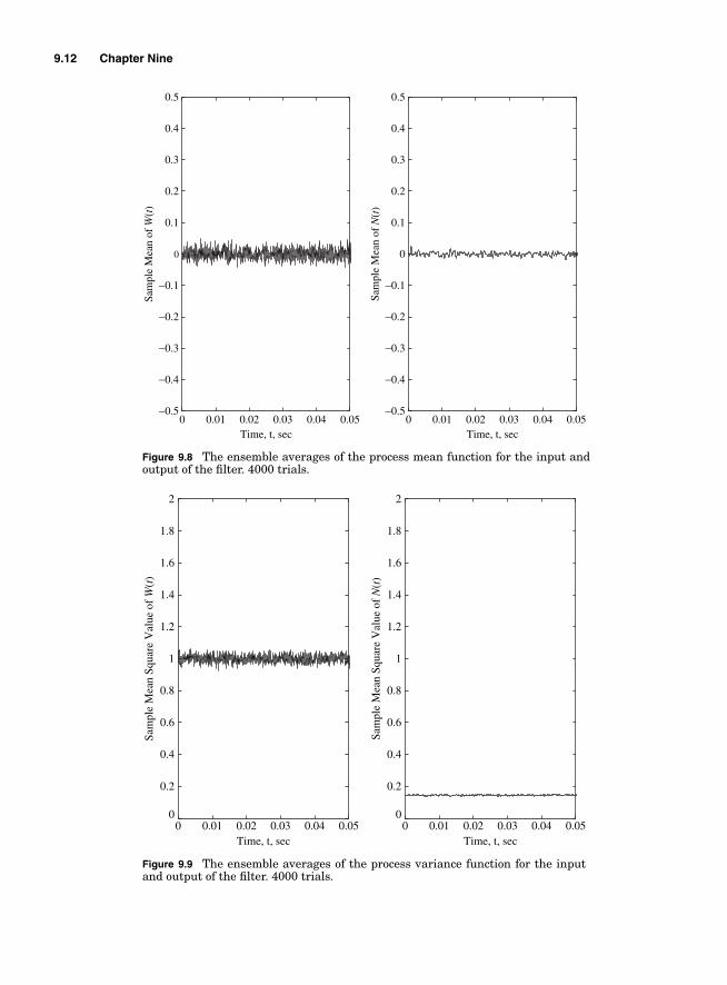
9.12 Chapter Nine
0 0.01 0.02 0.03 0.04 0.05−0.5
−0.4
−0.3
−0.2
−0.1
0
0.1
0.2
0.3
0.4
0.5
Time, t, sec
Sam
ple
Mea
n of
W(t
)
0 0.01 0.02 0.03 0.04 0.05−0.5
−0.4
−0.3
−0.2
−0.1
0
0.1
0.2
0.3
0.4
0.5
Time, t, sec
Sam
ple
Mea
n of
N(t
)
Figure 9.8 The ensemble averages of the process mean function for the input andoutput of the filter. 4000 trials.
0 0.01 0.02 0.03 0.04 0.050
0.2
0.4
0.6
0.8
1
1.2
1.4
1.6
1.8
2
Time, t, sec
Sam
ple
Mea
n Sq
uare
Val
ue o
f W
(t)
0 0.01 0.02 0.03 0.04 0.050
0.2
0.4
0.6
0.8
1
1.2
1.4
1.6
1.8
2
Time, t, sec
Sam
ple
Mea
n Sq
uare
Val
ue o
f N
(t)
Figure 9.9 The ensemble averages of the process variance function for the inputand output of the filter. 4000 trials.

Random Processes 9.13
that the processes in the canonical problem are stationary processes, since the meanand variance appear to be constant functions of time. The sample mean and variance ofthe processes match the histograms in Figure 9.4.
The correlation function gives a description of how rapidly the random processis changing with time. For a stationary random process the correlation functioncan be expressed as
RN (τ ) = σ 2N ρN (τ ) (9.15)
where ρN (τ ) is the correlation coefficient between two samples taken τ secondsapart. Recall that if ρN (τ ) ≈ 0 then the two samples will behave statisticallyin an independent fashion. If ρN (τ ) ≈ 1 then the two samples will be very closein value (statistically dependent). In addition to giving an engineer an idea ofhow rapidly the random process varies as a function of time, the correlationfunction also fully specifies the PDF of any number of samples from a Gaussianrandom process. Recall the quantities needed to specify the PDF of zero mean,jointly Gaussian random variables are the variance which is constant given as
σ 2N = RN (0) (9.16)
and the correlation coefficient between the random variables. The correlationcoefficient between the random variables N (t) and N (t − τ ) is given as
ρN (τ ) = RN (τ )σ 2
N(9.17)
Consequently for a zero mean, stationary Gaussian process the correlation func-tion completely determines the statistical characteristics of the process.
The idea of a correlation function has been introduced before in the context ofdeterministic signal analysis. For deterministic signals the correlation functionof a signal x(t) was defined as
Vx(τ ) =∞∫
−∞x(t)x∗(t − τ )dt (9.18)
This correlation function also was a measure of how rapidly a signal variedin time just like the correlation function for random processes measures thetime variations of a noise. Table 9.1 summarizes the comparison between thecorrelation functions for random processes and deterministic energy signals.

9.14 Chapter Nine
TABLE 9.1 Summary of the important characteristics of the correlation function
Signal Definition Units Correlation value at τ = 0
Deterministic Vx(τ ) =∞∫
−∞x(t)x∗(t − τ )dt Joules Vx(0) = Ex (Energy of x(t))
Random RN (τ ) = E[N (t)N (t − τ )] Watts RN (0) = σ 2N (Average power of N (t))
EXAMPLE 9.11Consider a correlation coefficient parameterized as
ρN (τ ) = sinc(2W τ ) (9.19)
For two samples taken τ = 250 µs apart, a process characterized with W = 400 Hz wouldhave these samples behaving very similar (ρN (.00025) = 0.935). A process characterizedwith W = 6400 Hz would have ρN (.00025) = −0.058 and essentially the two sampleswill be independent. Figure 9.10 shows a plot of several sample functions of Gaussian
0.025 0.0251 0.0251 0.0252 0.0252 0.0253 0.0253 0.0254 0.0254 0.0255−1.5
−1
−0.5
0
0.5
1
1.5
Time, t, sec
N(t
)
BW = 6400 HzBW = 1600 HzBW = 400 Hz
Figure 9.10 Sample paths for several Gaussian random processes parameterized by Eq. (9.19).Note this plot show samples of random processes where the sample rate is f s = 44, 100 Hz. Thejaggedness and piecewise linear nature of the high bandwidth noise is due to this sampling. Ahigher sampling rate would result in a smoother appearance.

Random Processes 9.15
0.023 0.024 0.025
(a) W = 6400 Hz.
0.026 0.027−1.5
−1
−0.5
0
0.5
1
1.5
Time, t, sec
N(t)RN(τ-0.025)
−1
−0.5
0
0.5
1
1.5N(t)RN(τ-0.025)
0.023 0.024 0.025
(b) W = 1600 Hz.
0.026 0.027−1.5
Time, t, sec
Figure 9.11 Sample paths of a stationary Gaussian process along with the associated correlation function.
random processes whose correlation function is given Eq. (9.19) with different values ofW . The process parameterized with W = 6400 Hz varies rapidly over 250 µs, while theprocess parameterized with W = 400 Hz is nearly constant. Another way to view therelation between the correlation function and the time variability of the random processintuitively is to plot sample paths of the random process along with the correlationfunction. Examples of this type of plot are shown in Figure 9.11 for W = 6400 Hz andW = 1600 Hz. This type of plot clearly highlights how the correlation function relatesto the variability of a random process; the narrower the correlation function the fasterthe random process varies in time.
Point 3: When the noise, N (t), is a stationary Gaussian random processthe canonical problem can be solved solely by knowing the form of RN (τ ) =E[N (t)N (t − τ )] as the PDF of any number of samples taken arbitrarilyfrom the process N (t) can be determined from RN (τ ).
9.3.3 Frequency Domain Representation
Stationary noise can also be described in the frequency domain. Frequencydomain analysis has been very useful for providing an alternate view (comparedto time domain) in deterministic signal analysis. This characteristic holds truewhen analyzing stationary random processes. Recall the definition of a finitetime Fourier transform given in Eq. (2.8), i.e.,
NTm( f , ω) =∫ Tm
−Tm
N (t, ω) exp[− j 2π f t]dt (9.20)

9.16 Chapter Nine
The finite time Fourier transform is a complex random function of frequency.Since N (t) is a stationary random process the energy of N (t) grows unboundedas the measurement interval, Tm, gets large. Because of the unbounded energyit proves useful to examine the finite time measured power spectral density(units Watts per Hertz), which is given as
SN ( f , ω, Tm) = 12Tm
|NTm( f , ω)|2 (9.21)
It should be noted that the finite time measured power spectral density is nowa real random function of frequency. In analogy to the energy spectrum, Gx(f ),introduced in Chapter 2, the measured power spectral density gives a distribu-tion of power in the frequency domain for the sample path N (t, ω). StationaryGaussian random processes are characterized in the frequency domain by theaverage power spectral density. The average of the measured power spectraldensity is given as
SN ( f , Tm) = 12Tm
E[|NTm( f , ω)|2] = E[SN ( f , ω, Tm)] (9.22)
and the limit as the measurement time gets large of this average is known asthe power spectral density of a stationary random process.
Definition 9.5 The power spectral density of a random process N (t) is
SN (f ) = limTm→∞
SN ( f , Tm)
Since the power spectral density is obtained by taking the ensemble averageand the time average of the energy spectrum of the sample paths, the powerspectral density is a measure of how the average power of the process is dis-tributed as a function of frequency. The characteristics of the power spectraldensity of stationary random signals, SN (f ), will parallel that of the energyspectral density of deterministic signals, GX (f ). Intuitively, random processesthat vary rapidly must have power at higher frequencies in a very similar wayas deterministic signals. This definition of the power spectral density puts thatintuition on a solid mathematical basis.
Property 9.7 The power spectrum of a real valued1 random process is always a nonnega-tive and an even function of frequency, i.e., SN (f ) ≥ 0 and SN (f ) = SN (− f ).
Proof: The positivity of SN (f ) is a direct consequence of Definition 9.5 andEq. (9.22). The evenness is due to Property 2.4. �
1This chapter only considers real valued random processes but the next chapter will extend theseideas to the complex envelope of a bandpass noise, hence the need to distinguish between a realand a complex random process.

Random Processes 9.17
−1−0.8 −0.6 −0.4 −0.2 0
(a) A sample path, SN(f, wi, Tm)
0.2 0.4 0.6 0.8 1× 10⁴
−100
−90
−80
−70
−60
−50
−40
−30
−20
Frequency, f, Hz
S N(f
,w,T
m)
−1 −0.8 −0.6 −0.4 −0.2 0
(b) Average of 4000 sample path, SN (f, Tm)
0.2 0.4 0.6 0.8 1× 10⁴
−100
−90
−80
−70
−60
−50
−40
−30
−20
Frequency, f, Hz
S N(f
,Tm
)Figure 9.12 A sample path and the average of 4000 sample paths.
EXAMPLE 9.12For the output random process defined in Example 9.2, sample power spectra, SN ( f , ω,Tm), can be computed from one sample path. Insight into the ensemble average can becomputed by looking at the sample mean of this function, i.e.,
SN ( f , Tm) = 1N
N∑i=1
SN ( f , ωi , Tm) (9.23)
Figure 9.12 shows one sample path, SN ( f , ωi , Tm), and the average of the sample paths,SN ( f , Tm), for 4000 samples paths. This is empirical evidence that SN (f ) is well definedand exists for this canonical process that is the focus of this chapter.
Spectral analysis of stationary random processes proves extremely valuablebecause the power spectral density is related to the correlation function as aFourier transform pair.
Property 9.8 (Wiener-Khinchin) The power spectral density for a stationary randomprocess is given by
SN (f ) = F{RN (τ )}
Proof: The power spectral density (see Definition 9.5) can be rewritten as
SN (f ) = limTm→∞
12Tm
E[|NTm(f )|2]

9.18 Chapter Nine
Using the definition in Eq. (9.20) gives
E[|NTm(f )|2] = E
[∫ Tm
−Tm
N (t1) exp[− j 2π f t1]dt1
∫ Tm
−Tm
N (t2) exp[ j 2π f t2]dt2
]
=∫ Tm
−Tm
∫ Tm
−Tm
E[N (t1)N (t2)] exp[− j 2π f (t1 − t2)]dt1dt2 (9.24)
Making a change of variables τ = t1 − t2 and using the stationarity of N (t)reduces Eq. (9.24) to
E[|NTm(f )|2] = ∫ Tm
−Tm
∫ Tm−t2
−Tm−t2
RN (τ ) exp[− j 2π f τ ]d τdt2 (9.25)
Taking the limit gives the desired result. �
Actually the true Wiener-Khinchin theorem is a bit more general but thisform is all that is needed for this text. The Wiener-Khinchin theorem has utilityin communication system engineering because it implies that RN (τ ) can becomputed once SN (f ) is identified. This correspondence between RN (τ ) andSN (f ) implies that the statistical description of N (t) is fully characterizedwith SN (f ).
The power spectral density can be used to find the average power of a randomprocess with a direct analogy to Rayleigh’s energy theorem. Recall that
E[N (t)N (t − τ )] = RN (τ ) = F−1{SN (f )} =∫ ∞
−∞SN (f ) exp( j 2π f τ )df (9.26)
so that the total average power of a random process is given as
E[N 2(t)] = RN (0) = σ 2N =∫ ∞
−∞SN (f )df (9.27)
Equation (9.27) demonstrates that the average power of a random process isthe area under the power spectral density curve.
EXAMPLE 9.13If
RN (τ ) = σ 2N sinc(2W τ ) (9.28)
then
SN (f ) =
⎧⎨⎩
σ 2N
2W| f | ≤ W
0 elsewhere(9.29)
A random process having this correlation–spectral density pair has power uniformlydistributed over the frequencies from −W to W .

Random Processes 9.19
TABLE 9.2 Summary of the duality of spectral densities nonnegativity
Signal Definition Units Correlation Value at τ = 0
Deterministic Gx(f ) = F{Vx(τ )} J/Hz Vx(0) = Ex =∫ ∞
−∞ Gx(f )df Gx(f ) ≥ 0
Random SN (f ) = F{RN (τ )} W/Hz RN (0) = σ 2N =∫ ∞
−∞ SN (f )df SN (f ) ≥ 0
The duality of the power spectral density of random signals, SN (f ) and theenergy spectral density of deterministic energy signals, Gx(f ), is also strong.Table 9.2 summarizes the comparison between the spectral densities for ran-dom processes and deterministic energy signals.
Point 4: When the noise, N (t), is a stationary Gaussian random processthe canonical problem can be solved with knowledge of the power spectraldensity of the random process, SN (f ). The power spectral density determinesthe correlation function, RN (τ ) through an inverse Fourier transform. Thecorrelation function completely characterizes any joint PDF of samples ofthe process N (t).
9.4 Thermal Noise
An additive noise is characteristic of almost all communication systems. Thisadditive noise typically arises from thermal noise generated by random motionof electrons in conductors. From the kinetic theory of particles, given a resistorR at a physical temperature of T degrees Kelvin, there exists a random additivenoise voltage, W (t), across the resistor. This noise is zero mean, stationary2, andGaussian distributed (due to the large number of randomly moving electronsand the central limit theorem), with a spectral density given as [Zie86, Joh28,Nyq28b]
SW (f ) = 2Rh| f |exp[
h| f |KT
]− 1
(9.30)
where h = 6.62 × 10⁻³⁴ is Planck’s constant and K = 1.3807 × 10⁻²³ is Boltz-mann’s constant. A plot of the power spectral density of thermal noise is shownin Figure 9.13. The major characteristic to note is that this spectral density isconstant up to about 1012 Hz at a value of 2KTR. Since Johnson [Joh28] mademeasurements to characterize the thermally generated noise in conductors andNyquist [Nyq28b] provided the theory that matched these measurements, ther-mal noise is often known as Johnson noise or Johnson–Nyquist noise.
2As long as the temperature is constant.

9.20 Chapter Nine
−240
−235
−230
−225
−220
−215
−210
−205
1 100 104 106 108 1010 1012 1014 1016 1018
S W(f
), d
BW
/Hz
Frequency, f, Hz
Figure 9.13 The PSD of thermal noise.
Since a majority of communications occurs at frequencies much lower than1012 Hz3 an accurate and simplifying model of the thermal noise is to assumea flat spectral density (white noise). This spectral density is a function of thereceiver temperature. The lower the temperature of the receiver the lower thenoise power. Additive white Gaussian noise (AWGN) is a basic assumptionmade about the corrupting noise in most communication systems performanceanalyses. White noise has a constant spectral density given as
SW (f ) = N0
2(9.31)
where N0/2 is the noise power spectral density. Note that since
E[W 2(t)] =∫ ∞
−∞SW (f )df (9.32)
this thermal noise model has an infinite average power. This characteristic isonly a result of modeling Eq. (9.30) with the simpler form in Eq. (9.31). Tra-ditionally some engineers have been loath to admit to the idea of negativefrequencies hence they are not comfortable with the model in Eq. (9.31). Theseengineers like to think about noise power distributed over positive only fre-quencies with a spectral density of double the height. In the literature one willoften see people denote N0/2 as the two-sided noise spectral density and N0 asthe one-sided noise spectral density.
3Fiber optic communication is a notable exception to this statement.

Random Processes 9.21
The autocorrelation function of AWGN is given by
RW (τ ) = E[W (t)W (t − τ )] = N0
2δ(τ ) (9.33)
AWGN is a stationary random process so a great majority of the analysis incommunication systems design can utilize the extensive theory of stationaryrandom processes. White noise has the interesting characteristic that two sam-ples of the process W (t) will always be independent no matter how closely thesamples are taken. Consequently, white noise can be thought of as a very rapidlyvarying noise with no predictability.
A resistor in isolation will produce an approximate white noise with a two-sided spectral density of 2KTR. If this system is placed in an electronic system,the greatest value of the average power that would be able to be transferredout of the resistor is one fourth of value that would exist if the resistor wasshorted (using the maximum power transfer theorem of linear systems, seeProblem 9.13). Hence an important number for communication system engi-neers to remember is N0 = KT . For room temperature (T = 290◦K ) N0 =4 × 10⁻²¹ W/Hz (−174 dBm/Hz). When signals get amplified by active com-ponents in a receiver the value of this noise spectral density will change. Weexplore some of these ideas in the homework and refer the interested student tothe detailed references [Zie86, Cou93, Skl88] on the ideas of noise figure, linkbudgets, and computing output signal to noise ratio.
This noise spectral density at the input to a communication system is verysmall. If this thermal noise is to corrupt the communication signal then thesignal must also take a small value. Consequently, it is apparent from thisdiscussion that thermal noise is only going to be significant when the signal atthe receiver has been attenuated to a relatively small power level.
EXAMPLE 9.14The noise plotted in Figure 9.7(b) could result from sampling of an wideband noise at asample rate of f s = 22, 050 Hz. The rapidly varying characteristic of the noise samplespredicted by Eq. (9.33) is evident from Figure 9.7(b). A sample path of the measuredpower spectrum and the average of 4000 trials of this experiment (see Eq. (9.22)) forthis process is shown in Figure 9.14. This average spectrum clearly shows the whitenoise model for the PSD is appropriate. Figure 9.15 shows the histogram of the samplesof the AWGN. The Gaussian nature of this histogram is also clearly evident. In a vastmajority of communication system analysis the model of a AWGN is very accurate andused in practice.
Point 5: The dominant noise in communication systems is often generated bythe random motion of electrons in conductors. This noise process is accuratelymodeled as stationary, Gaussian, and white.

9.22 Chapter Nine
−1 −0.8 −0.6 −0.4 −0.2 0 0.2 0.4 0.6 0.8 1
× 104
−100
−90
−80
−70
−60
−50
−40
−30
−20
Frequency, f, Hz(a) The measured PSD of a sample path.
S N(f
,w,T
m)
−1−0.8−0.6 −0.4 −0.2 0
(b) The average of the measured PSD, 4000 trials.
0.2 0.4 0.6 0.8 1
× 104
−100
−90
−80
−70
−60
−50
−40
−30
−20
Frequency, f, HzS N
(f,T
m)
Figure 9.14 Spectral characteristics of sampled wideband Gaussian noise.
−4 −3 −2 −1 0 1 2 3 40
50
100
150
200
250
300
Values of W(t)
Num
ber
of O
ccur
renc
es
Figure 9.15 The measured histogram of wideband Gaussian noise, 4000 trials.

Random Processes 9.23
9.5 Linear Systems and Random Processes
The final step in solving the canonical problem is to characterize the output ofa linear time-invariant filter when the input is a stationary, white, Gaussianrandom process.
Property 9.9 Random processes that result from linear filtering of Gaussian randomprocesses are also Gaussian processes.
Proof: The technical machinery needed to prove this property is beyond thescope of this class but most advanced texts concerning random processes willprove this. For example [DR87]. It should be noted that a majority of the im-portant ideas used in this proof can be understood by examining Problem 3.24.
�
Property 9.10 A random process that results from linear filtering of a zero mean processwill also be zero mean.
Proof: Assume the filter input is W (t), the filter impulse response is hR(t), andthe filter output is N (t).
E[N (t)] = E[∫ ∞
−∞hR(λ)W (t − λ)dλ
]=∫ ∞
−∞hR(λ)E[W (t − λ)]dλ = 0. (9.34)
�
Property 9.11 A Gaussian random process that results from linear time-invariant fil-tering of another stationary Gaussian random process is also a stationary Gaussianprocess.
Proof: Assume the filter input is W (t), the filter impulse response is hR(t), andthe filter output is N (t). Since we know the output is Gaussian, the stationarityof N (t) only requires that the correlation function of N (t) be a function of τ
only, i.e., RN (t1, t2) = RN (τ ). The two argument correlation function of N (t) isgiven as
RN (t1, t2) = E[N (t1)N (t2)]
= E[∫ ∞
−∞hR(λ1)W (t1 − λ1)dλ1
∫ ∞
−∞hR(λ2)W (t2 − λ2)dλ2
](9.35)
Rearranging gives
RN (t1, t2) =∫ ∞
−∞hR(λ1)
∫ ∞
−∞hR(λ2)E[W (t1 − λ1)W (t2 − λ2)]dλ1dλ2
=∫ ∞
−∞hR(λ1)
∫ ∞
−∞hR(λ2)RW (t1 − λ1 − t2 + λ2)dλ1dλ2
=∫ ∞
−∞hR(λ1)
∫ ∞
−∞hR(λ2)RW (τ − λ1 + λ2)dλ1dλ2
= g(τ ). (9.36)
�

9.24 Chapter Nine
Point 6: The output noise in the canonical problem, N (t), is accurately mode-led as a stationary Gaussian process.
The canonical problem given in Figure 9.1 can now be solved by finding the cor-relation function or spectral density of the stationary Gaussian random processN (t). For the canonical problem W (t) is a white noise so that Eq. (9.36) can berewritten as
RN (τ ) =∫ ∞
−∞hR(λ1)
∫ ∞
−∞hR(λ2)
N0
2δ(λ1 − λ2 − τ )dλ1dλ2 (9.37)
Using the sifting property of the delta function gives
RN (τ ) = N0
2
∫ ∞
−∞hR(λ1)hR(λ1 − τ )dλ1 = N0
2VhR (τ ) (9.38)
where VhR (τ ) is the correlation function of the deterministic impulse responsehR(t) as defined in Chapter 2. This demonstrates that the output correlationfunction from a linear filter with a white noise input is only a function of thefilter impulse response and the white noise spectral density.
The frequency domain description of the random process N (t) is equallysimple. The power spectral density is given as
SN (f ) = F{RN (τ )} = N0
2F{VhR (τ )} = N0
2GhR (f ) = N0
2|HR(f )|2 (9.39)
The average output noise power is given using either Eq. (9.38) or Eq. (9.39) as
σ 2N = E[N 2(t)] = RN (0) = N0
2
∫ ∞
−∞|HR(f )|2df = N0
2
∫ ∞
−∞|hR(t)|2dt (9.40)
It should be noted that Eq. (9.40) is another example of Parseval’s theorem insignal analysis.
The result in Eq. (9.39) is a special case of a more general result. The generalresult is
SN (f ) = SW (f )|HR(f )|2 = SW (f )GhR (f ) (9.41)
This can be obtained by taking the Fourier transform of Eq. (9.36) as this dou-ble integral can be reformulated as a double convolution. It is clear that bysubstituting SW (f ) = N0/2 into Eq. (9.41) gives the result in Eq. (9.39). Con-sequently, the output spectral density of a linear time-invariant filter is equalto the product of the input power spectral density and the energy spectrum ofthe impulse response (the magnitude squared of the transfer function). Thischaracteristic enables an easy characterization of the impact of a filter in thefrequency domain.
EXAMPLE 9.15This example considers the sampled wideband Gaussian noise shown in Figure 9.7(b)being put into a lowpass filter of bandwith 1600 Hz. This lowpass filter will significantly

Random Processes 9.25
0.046 0.047 0.048 0.049 0.050 0.051 0.052 0.053 0.054−3
−2
−1
0
1
2
3
Time, t, sec
W(t)N(t)
Figure 9.16 Sample paths of wideband and filtered noise. Filter bandwidth =1600 Hz.
smooth out the sampled noise and reduce the variance of the output process. Two samplefunctions; one for the input wideband noise and one for the filtered noise, are shown inFigure 9.16. The lowering of the output power of the noise and the smoothing in thetime variations that is expected to be produced at the lowpass filter output are readilyapparent in this figure. The output measured PSD of the filtered noise is shown inFigure 9.17(b). This measured PSD validates Eq. (9.39), as this PSD is clearly the resultof multiplying the measured input noise spectral density (modeled in the text as awhite noise) with the lowpass filter energy spectrum as seen in Figure 9.17(a). This isanother great example in communication engineering where the theory exactly predictsthe measurement and why the theory has found such utility in practice. As a final point,the histogram of the output samples, shown in Figure 9.18, again demonstrates that theoutput noise is well modeled as a zero mean Gaussian random process.
EXAMPLE 9.16Consider an AWGN with a one-sided spectral density of N0 being input into an ideallowpass filter of bandwidth W , i.e.,
HR(f ) ={
1 | f | ≤ W
0 elsewhere(9.42)

9.26 Chapter Nine
−1 −0.8 −0.6 −0.4 −0.2 0
(a) Sample average PSD of W(t) and Gh( f ), 4000 trials.
0.2 0.4 0.6 0.8 1
× 104 × 104
−80
−70
−60
−50
−40
−30
−20
−10
0
10
Frequency, f, Hz
Spec
tra
SW(f)
Gh(f)
−1 −0.8 −0.6 −0.4 −0.2 0
(b) Sample average PSD of N(t), 4000 trials.
0.2 0.4 0.6 0.8 1−120
−110
−100
−90
−80
−70
−60
−50
−40
Frequency, f, Hz
S N(f
,ω, T
m)
Figure 9.17 Measured spectral characteristics of filtered wideband noise.
−1.5 −1 −0.5 0 0.5 1 1.50
50
100
150
200
250
300
Values of N(t)
Num
ber
of O
ccur
renc
es
Figure 9.18 A histogram of the samples of the filtered noise.

Random Processes 9.27
The output spectral density is given as
SN (f ) =
⎧⎨⎩
N0
2| f | ≤ W
0 elsewhere(9.43)
and the average output power is given as σ 2N = N0W .
Engineers noted the simple form for the average output noise power expressionin Example 9.16 and decided to parameterize the output noise power of all filtersby a single number, the noise equivalent bandwidth.
Definition 9.6 The noise equivalent bandwidth of a filter is
BN = 12|HR(0)|2
∫ ∞
−∞|HR(f )|2df
For an arbitrary filter the average output noise power will be σ 2N = N0 BN
|HR(0)|2. Note, for a constant |HR(0)| the smaller the noise equivalent band-width the smaller the noise power. This implies that noise power can be mini-mized by making BN as small as possible. In the homework problems we willshow that the output signal to noise ratio is not a strong function of |HR(0)|so that performance in the presence of noise is well parameterized by BN. Ingeneral, HR(f ) is chosen as a compromise between complexity of implementa-tion, signal distortion, and noise mitigation.
Point 7: A stationary, white, and Gaussian noise of two-sided spectral den-sity N0/2 when passed through a filter will produce a stationary Gaussiannoise whose power spectral density is given as
SN (f ) = N0
2|HR(f )|2
9.6 The Solution of the Canonical Problem
Putting together the results of the previous five sections leads to a solution ofthe canonical problem posed in this chapter.
First, the characterization of one sample, N (ts), of the random process N (t)is considered. This case requires a four step process summarized as
1. Identify N0 and HR(f ).
2. Compute SN (f ) = N02 |HR(f )|2.
3. σ 2N = E[N 2(t)] = RN (0) = N0
2
∫∞−∞ |HR(f )|2df = N0 BN |HR(0)|2
4. fN (ts)(n1) = 1√2πσ 2
N
exp(− n2
12σ 2
N
)

9.28 Chapter Nine
EXAMPLE 9.17Consider two ideal lowpass filters with
HR(i)(f ) ={
1 | f | ≤ Wi
0 elsewhere(9.44)
with W1 = 400 Hz and W2 = 6400 Hz and a noise spectral density of
N0 = 11600
Step 2 gives
SNi (f ) =
⎧⎨⎩
13200
| f | ≤ Wi
0 elsewhere(9.45)
Step 3 gives σ 2N1
= 0.25 and σ 2N2
= 4. The average noise power between the two filteroutputs is different by a factor of 16. The PDFs in step 4 are plotted in Figure 9.19.
Second, the characterization of two samples, N (t1) and N (t2), of the randomprocess N (t) is considered. This case requires a five step process summarizedas
1. Identify N0 and HR(f ).
2. Compute SN (f ) = N02 |HR(f )|2.
0
0.1
0.2
0.3
0.4
0.5
0.6
0.7
0.8
−4 −3 −2 −1 0 1 2 3 4
W = 6400
W = 400
f N(t
)(n s
)
ns
Figure 9.19 The PDF of a filter output sample for W = 400 and W = 6400 Hz.

Random Processes 9.29
3. RN (τ ) = F−1{SN (f )}4. σ 2
N = RN (0) and ρN (τ ) = RN (τ )/σ 2N
5. fN (t1)N (t2)(n1, n2) = 12πσ 2
N
√(1−ρN (τ )2)
exp[
−12σ 2
N (1−ρN (τ )2)
(n2
1 − 2ρN (τ )n1n2 + n22
)]
EXAMPLE 9.18Consider two ideal lowpass filters with
HR(i)(f ) ={
1 | f | ≤ Wi
0 elsewhere(9.46)
with W1 = 400 Hz and W2 = 6400 Hz and a noise spectral density of
N0 = 11600
Step 2 gives
SNi (f ) =
⎧⎨⎩
13200
| f | ≤ Wi
0 elsewhere(9.47)
Step 3 gives RN1 (τ ) = 0.25sinc(800τ ) and RN2 (τ ) = 4sinc(12,800τ ). Step 4 has theaverage noise power between the two filter outputs being different by a factor of 16since σ 2
N1= 0.25 and σ 2
N2= 4. For an offset of τ seconds the correlation coefficients
are ρN1 (τ ) = sinc(800τ ) and ρN2 (τ ) = sinc(12,800τ ). The PDFs in step 5 are plottedin Figure 9.20(a) and Figure 9.20(b) for τ = 250 µs. With the filter having a band-width of 400 Hz the variance of the output samples is less and the correlation betweensamples is greater. This higher correlation implies that the probability that the tworandom variables take significantly different values is very small. This correlation is
−4−2 0
(a) W = 400 Hz. (b) W = 6400 Hz.
24
−4
−2
0
240
0.5
1
1.5
2
n1
f N(t
)N(t
+τ)
(n1,
n2)
n2
−4−2
02
4
−4
−2
0
240
0.01
0.02
0.03
0.04
n1
n2
f N(t
)N(t
+τ)
(n1,
n2)
Figure 9.20 The PDF of two samples separated by τ = 250 µs.

9.30 Chapter Nine
evident due to the knife edge like joint PDF. These two joint PDFs show the charac-teristics in an analytical form that were evident in the noise sample paths shown inFigure 9.10.
Similarly, three or more samples of the filter output could be characterizedin a very similar fashion. The tools developed in this chapter give a student theability to analyze many of the important properties of noise that are of interestin communication systems design.
9.7 Homework Problems
Problem 9.1. For this problem consider the canonical block diagram shown inFigure 9.21 with si(t) = cos(2π(200)t) and with W (t) being an additive whiteGaussian noise with two-sided spectral density of N0/2. Assume HR(f ) is anideal lowpass filter with bandwidth of 400 Hz. Two samples are taken from thefilter output at time t = 0 and t = τ , i.e., Yo(0) and Yo(τ ).
(a) Choose N0 such that the output noise power, E[N 2(t)] = 1.
(b) Yo(0) is a random variable. Compute E[Yo(0)] and E[Y 2o (0)], and var(Yo(0)).
(c) Yo(τ ) is a random variable. Compute E[Yo(τ )] and E[Y 2o (τ )], and var(Yo(τ )).
(d) Find the correlation coefficient between Yo(0) and Yo(τ ) i.e.,
ρYo (τ ) = E[(Yo(0) − E[Yo(0)])(Yo(τ ) − E[Yo(τ )])]√var(Yo(0))var(Yo(τ ))
(9.48)
(e) Plot the joint density function, f Yo(0)Yo(τ )(y1, y2), of these two samples forτ = 2.5 ms.
(f) Plot the joint density function, f Yo(0)Yo(τ )(y1, y2), of these two samples forτ = 25 µs.
(g) Compute the time average signal to noise ratio where the instantaneoussignal power is defined as E[Yo(t)]2.
Problem 9.2. Real valued additive white Gaussian noise (two-sided spectral den-sity N0/2) is input into a linear-time-invariant filter with a real valued impulseresponse hR(t) where hR(t) is constrained to have a unit energy (see Figure 9.21where si(t) = 0).
H fR( )s t W ti( ) ( )+ Y t s t N to o( ) ( ) ( )= +
Figure 9.21 Block diagram for signals, noise, and linearsystems.

Random Processes 9.31
(a) Calculate the output correlation function, RN (τ ).
(b) The output signal is sampled at a rate of f s. Give conditions on the im-pulse response, hR(t), that will make these samples independent. Give oneexample of a filter where the output samples will be independent.
(c) Give the PDF of one sample, e.g., fN (t1)(n1).
(d) Give the PDF of any two sample, e.g., fN (t1)N (t1+k/ f s)(n1, n2) where k is anonzero integer and the filter satisfies the conditions in (b).
(e) Give an expression for P (N (t1) > 2).
Problem 9.3. Real valued additive white Gaussian noise, W (t) with a two-sidedspectral density N0/2 = 0.1 is input into a linear-time-invariant filter with atransfer function of
H (f ) ={
2 | f | ≤ 10
0 elsewhere(9.49)
The output is denoted N (t).
(a) What is the correlation function, RW (τ ), that is used to model W (t)?
(b) What is E[N (t)]?
(c) Calculate the output power spectral density, SN (f ).
(d) What is E[N 2(t)]?
(e) Give the PDF of one sample, e.g., fN (t1)(n1).
(f) Give an expression for P (N (t1) > 3).
Problem 9.4. For this problem consider the canonical block diagram shown inFigure 9.21 with si(t) = A and with W (t) being an additive white Gaussiannoise with two-sided spectral density of N0/2. Assume a 1-� system and breakthe filter response into the DC gain term, HR(0) and the normalized filterresponse, HN (f ), i.e., HR(f ) = HR(0)HN (f ).
(a) What is the input signal power?
(b) What is the output signal power, Ps?
(c) What is the average output noise power, σ 2N ?
(d) Show that the output SNR = Ps/σ2N is not a function of HR(0).
(e) Give the output SNR as a function of A, N0, and BN.
Problem 9.5. For the canonical problem given in Figure 9.1, the output noisespectral density is given as
SN (f ) ={
N0 f 2 | f | ≤ W
0 elsewhere(9.50)

9.32 Chapter Nine
(a) What is the average ouput noise power?
(b) Give a possible HR(f ) that would result in this output noise?
(c) Think of a way to implement this HR(f ) using a lowpass filter cascadedwith another linear system that is used in the demodulation of an analogmodulation.
Problem 9.6. Show that SN (f ) = SW (f )|HR(f )|2 by taking the Fourier transformof Eq. (9.36).
Problem 9.7. Consider the following linear system with a signal, si(t), plus awhite Gaussian noise, W (t), as inputs.
Y (t) = so(t) + N (t) =∫ t
t−T i
x(λ)dλ =∫ t
t−T i
(si(λ) + W (λ))dλ (9.51)
where T i is defined as the integration time.
(a) What is the impulse response of this linear system, hr (t).
(b) Show that
σ 2N = N0
2
∫ ∞
−∞|hr (t)|2dt (9.52)
(c) If the input to the filter is a DC term plus the AWGN, i.e.,
Y (t) =∫ t
t−T i
( A+ W (λ))dλ (9.53)
find the output SNR= Ps/σ2N as a function of T i.
(d) For the case considered in (c) show that SNR grows monotonically with T i.
(e) If the input to the filter is a sinusoid signal plus the AWGN, i.e.,
Y (t) =∫ t
t−T i
(√
2Acos(2π fmt) + W (λ))dλ (9.54)
find the output SNR as a function of T i.
(f) For the case considered in (e) show that SNR does not grows monotonicallywith T i and find the optimum T i for each fm.
Problem 9.8. Real valued additive white Gaussian noise, W (t) with a two-sidedspectral density N0/2 = 0.1 is input into a linear-time-invariant filter with atransfer function of
HR(f ) ={
2 | f | ≤ W
0 elsewhere(9.55)
The output is denoted N (t).

Random Processes 9.33
(a) What is the correlation function, RW (τ ), that is used to model W (t)?
(b) What is E[N (t)]?
(c) Calculate the output power spectral density, SN (f ).
(d) Select W to give E[N 2(t)] = 10.
(e) Give the PDF of one sample, e.g., fN (t1)(n1) when E[N 2(t)] = 10.
(f) Given an expression for P (N (t1) > 3) when E[N 2(t)] = 10.
Problem 9.9. As simple model of a radar receiver consider the following problem.A radar sends out a pulse and listens for the return at the receiver whosefiltering is represented with an impulse response hR(t). The situation when notarget is present is represented with the input being modeled as a real valuedadditive white Gaussian noise, Y (t) = W (t), (W (t) has a two-sided spectraldensity N0/2) being input into a linear-time-invariant filter with a real valuedimpulse response hR(t). Denote the output as V (t). The situation where a targetis present can be represented as the same filter with a input Y (t) = A + W (t).A target detection decision is given by a simple threshold test at time t
V (t)Target Present
><
Target Absentγ (9.56)
(a) For the case when no target is present, completely characterize a sample ofthe process V (t).
(b) For a particular time t, find a value of the threshold, γ , where the probabilitythat a target will be declared present when one is not present is 10−5.
(c) For the case when a target is present completely characterize a sample ofthe process V (t).
(d) For the value of the threshold selected in (b) find how large A should be tocorrectly detect a target present with a probability of detection greater than0.9 for any value of t.
Problem 9.10. A real valued additive white Gaussian noise, W (t), (two-sided spec-tral density N0/2) is input into a linear-time-invariant filter with a real valuedimpulse response hR(t). Assume hR(t) represents an ideal lowpass filter withbandwidth BT and N (t) is the output of the filter.
(a) Find RN (τ ).
(b) Choose BT such that E[N 2(t)] = 1.
(c) For the random process Z(t) = N (t) − N (t − t1) find RZ(τ ).
(d) Select a value of t1 such that E[Z2(t)] = 0.5 for the BT computed in (b).
Problem 9.11. (Adapted from PD) Prof. Fitz likes to gamble but he is so busythinking up problems to torment students that he can never find time to get

9.34 Chapter Nine
to Las Vegas. So instead he decides to gamble with the students in his com-munication classes. The game has real valued additive white Gaussian noise(two-sided spectral density N0/2 = 1), W (t), input into a linear-time-invariantfilter with a real valued impulse response
hR(t) =
⎧⎪⎨⎪⎩
2 0 ≤ t ≤ 0.5
−2 0.5 < t ≤ 1
0 elsewhere
(9.57)
Prof. Fitz samples the noise, N (t), at a time of his choosing, t0, and notes thesign of the noise sample. The student playing the game gets to choose a latertime, t0 + τ, τ > 0 to sample the noise and if the sign of the noise sample is theopposite of Prof. Fitz’s sample then the student gets out of the final exam.
(a) Calculate the output correlation function, RN (τ ).
(b) Prof. Fitz samples at t0 = 1, find E[N 2(1)].
(c) Give the probability density function of Prof. Fitz’s sample, e.g., fN (t0)(n1).
(d) If you are playing the game and Prof. Fitz samples the noise at t0 = 1, selecta sample time to optimize your odds of getting out of the test. Justify youranswer. Could you do better if you were allowed to sample the process at atime before Prof. Fitz samples the process?
(e) If Prof. Fitz gets a realization N (1) = 2 in his sample, compute the proba-bility of your getting out of the test for the optimized sample time you gavein (d).
Problem 9.12. Consider the model in Figure 9.1 where the noise is zero meanwhite Gaussian with a one-sided noise spectral density of N0 W/Hz and filterhas an impulse response of
hR(t) ={
exp[−at] t ≥ 0
0 elsewhere(9.58)
where a > 0.
(a) Find E[N 2(ts)].
(b) Find P (N (ts) ≤ 1).
(c) Find the noise equivalent bandwidth of this filter, BN .
(d) Find P (N (ts + τ ) ≤ 0|N (ts) = 1). Hint: Eq. (3.23) might be useful.
Problem 9.13. Noise in communication systems are often modeled with the sys-tem in Figure 9.22. The noise source consists of an ideal voltage noise sourceand a source resistance. If the noise source produces a voltage of N (t) whereN (t) is a stationary noise with E[N 2(t)] = PN .

Random Processes 9.35
+
−N t( )
Rs
R
SinkSource
Figure 9.22 A noise source and sink.
(a) Find the average power delivered to the sink as a function of Rs and R.
(b) What is the value of R that would maximize this power and what would bethe corresponding maximum average power delivered.
Problem 9.14. Given Figure 9.23 and W (t) being an additive white Gaussiannoise (RW (τ ) = N0/2δ(τ )).
(a) Express the probability density function (PDF) of the random variable N1(t1)for a fixed t1 in terms of h1(t) and N0.
(b) Find the E[N1(t1)N2(t1)] for a fixed t1 in terms of h1(t), h2(t), and N0. Specifythe joint PDF of N1(t1) and N2(t1).
(c) If h1(t) is given in Figure 9.24 then find an impulse response for h2(t) suchthat N1(t1) and N2(t1) for a fixed t1 are independent random variables withequal variances Hint: The answer is not unique.
Problem 9.15. For this problem consider the canonical block diagram shown inFigure 9.21 with si(t) = Acos(200πt) and with W (t) being an additive whiteGaussian noise with two-sided spectral density of N0/2 = 0.01. HR(f ) is a filterwith a transfer function given in Figure 9.25.
(a) What is so(t) and what is Pso?
(b) If two samples are taken from W (t), e.g., W (t1) and W (t2), what spacing inthe time samples, t2 − t1, must be maintained to have two samples that arestatistically independent random variables?
W t( )
h t1( )
h t2( ) N t2( )
N t1( )
Figure 9.23 White noise into a linear filter,4000 trials.

9.36 Chapter Nine
Tp
1
h t1( )
t
Figure 9.24 An example impulseresponse.
(c) What is the spectral density of N (t), SN (f )?
(d) What is the noise power, E[N 2(t)]?
(e) Choose A such that the output SNR = 10.
Problem 9.16. Consider the model in Figure 9.1 where the noise is zero meanwhite Gaussian with a one-sided noise spectral density of N0 W/Hz and filteris an ideal bandpass filter of bandwidth BT that has a transfer function of
HR(f ) ={
3 f c − BT2 ≤ | f | ≤ f c + BT
2
0 elsewhere(9.59)
Assume f c ≥ BT .
(a) Find SN (f ).
(b) Find E[N 2(ts)].
(c) Find RN (τ ).
(d) Find P (N (ts) ≤ 1).
(e) Find P (N (ts + τ ) ≤ 0|N (ts) = 1). Hint: Eq. (3.23) might be useful.
(f) Find the value of τ that maximizes P (N (ts + τ ) ≤ 0|N (ts) = 1).
H fR( )
f
1
200 400
Figure 9.25 Transfer function of HR(f ).
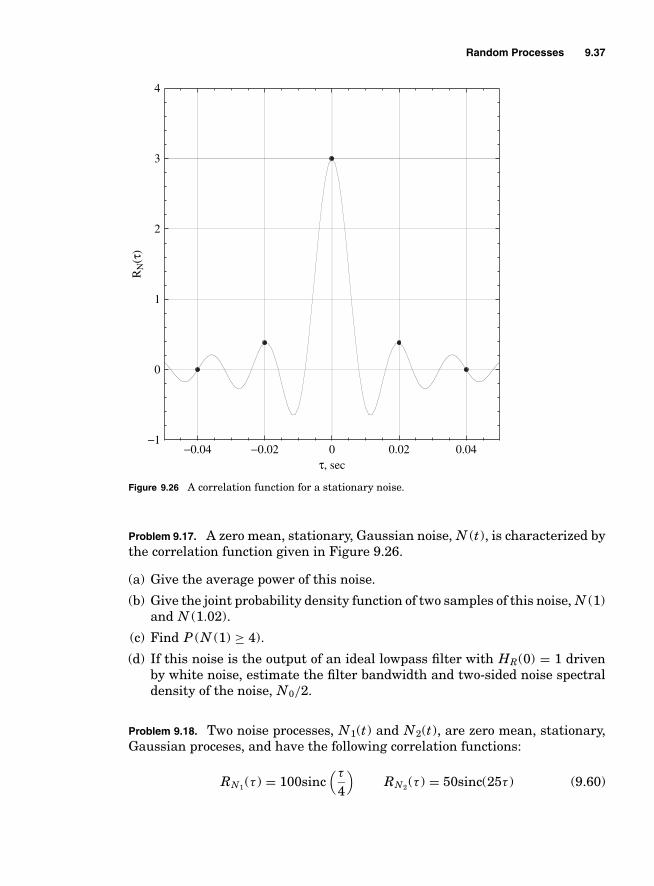
Random Processes 9.37
−1
0
1
2
3
4
−0.04 −0.02 0 0.02 0.04
RN
(τ)
τ, sec
Figure 9.26 A correlation function for a stationary noise.
Problem 9.17. A zero mean, stationary, Gaussian noise, N (t), is characterized bythe correlation function given in Figure 9.26.
(a) Give the average power of this noise.
(b) Give the joint probability density function of two samples of this noise, N (1)and N (1.02).
(c) Find P (N (1) ≥ 4).
(d) If this noise is the output of an ideal lowpass filter with HR(0) = 1 drivenby white noise, estimate the filter bandwidth and two-sided noise spectraldensity of the noise, N0/2.
Problem 9.18. Two noise processes, N1(t) and N2(t), are zero mean, stationary,Gaussian proceses, and have the following correlation functions:
RN1 (τ ) = 100sinc(τ
4
)RN2 (τ ) = 50sinc(25τ ) (9.60)

9.38 Chapter Nine
W t1( )
W t2( )
h t1( )
h t2( )
h t3( ) E t( )
N t1( )
N t2( )
N t( )+
−Σ Σ
Figure 9.27 A system block diagram.
(a) Which random process has a greater power? Why?
(b) Two samples are taken from N2(t), N2(t1), and N2(t1+τ ). What is the small-est value of τ such that the two samples are orthogonal random variables?
(c) For N1(t), what is the correlation coefficient corresponding to τ = 1? Givethe joint PDF of two samples of N1(t) taken 1 second apart.
(d) Find P (N1(t) < −10).
(e) Using only linear devices (amplifiers and filters), generate a random processstatistically identical to N1(t) from N2(t).
Problem 9.19. Consider the block diagram in Figure 9.27 where Wi(t) are inde-pendent white Gaussian noises with RWi (τ ) = N0/2δ(τ ), i = 1, 2.
(a) Find fN (t0)(n).
(b) Find P (N (t0) > −1).
(c) Find fN (t0)N (t0−τ )(n1, n2).
(d) Find fN (t0)(n|N (t0 − τ ) = n1).
(e) Find the simplest expression for SE (f ).
Problem 9.20. Two random processes are defined as
N1(t) = X cos(2π fot) + Y (9.61)
and
N2(t) = X cos(2π fot) + Y sin(2π fot) (9.62)
where X and Y are independent zero mean jointly Gaussian random variableswith unity variance and fo is a deterministic constant.
(a) Are these processes Gaussian processes?
(b) For each of the processes that are Gaussian given a joint density functionof the samples of the random process taken at t = 0 and t = 1/(4 fo).
(c) Are these processes stationary? Hint: Trigonometry formulas will be usefulhere.

Random Processes 9.39
ThermalNoise
W(t) N(t)HR( f )
Figure 9.28 The noise model.
Problem 9.21. Consider an additive white Gaussian noise input into a linear-time-invariant system as given in Figure 9.28. Suppose that
HR(f ) ={
A | f | ≤ W
0 elsewhere(9.63)
and that SW (f ) = N02 .
(a) Choose A such that σ 2N (t) = 1.
(b) If W = 100 Hz and N (t0) = 2 find the conditional mean E[N (t0 − τ )|N (t0) = 2]. Hint: See Section 3.3.3.
(c) If W = 100 Hz, N (t0) = 2, and τ > 0.01 find the value of τ that will minimize
var(N (t0 − τ )|N (t0) = 2) (9.64)
Problem 9.22. Often in engineering practice message signals are modeled as ran-dom processes. Assume M(t) is a Gaussian random process with the powerspectrum given in Figure 9.29.
(a) What is the power of this signal, Pm?
(b) Find the PDF of one sample of this message signal.
(c) What is the correlation function of the message signal, RM(τ )?
(d) Find and plot the PDF of two samples of this message signal taken τ =1/200 seconds apart.
(e) Find and plot the PDF of two samples of this message signal taken τ =0.25/200 seconds apart.
f
1
200−200
S fM( )
Figure 9.29 The power spectrum of the message signal.

9.40 Chapter Nine
Problem 9.23. This chapter came to the conclusion that noise in a communica-tion system is well modeled as Gaussian and stationary. In a similar modelingexercise provide a detailed justification of whether it is appropriate to modelthe following random processes as Gaussian and/or stationary
(a) The number of victories in a year for the Ohio State University men’sAmerican football team
(b) The number of skiers per day at the Vail Colorado ski resort
(c) The number of oxygen molecules in one liter of air in your classroom
(d) The number of women engineers graduating from Purdue University in ayear
(e) The number of cars per hour passing a point on a Los Angeles freeway
Problem 9.24. Consider a model with a zero mean Gaussian and stationary noise,N1(t), input into a linear filter with an impulse response h(t) and a transferfunction of H (f ). Denote the output noise N2(t).
(a) Show that the cross–correlation between the input and the output of thefilter is given as
RN1 N2 (τ ) = E[N1(t)N2(t − τ )] =∫ ∞
−∞RN1 (τ + λ)h(λ)dλ (9.65)
(b) Show the cross spectrum between the input and output is
SN1 N2 (f ) = F{RN1 N2 (τ )} = SN1 (f )H ∗(f ) (9.66)
Problem 9.25. Active electronic devices produce more noise than passive devices(e.g., a resistor) and this can decrease the output SNR from the device. An idealmodel of an amplifier in a communication system is given in Figure 9.30.
(a) In the ideal model of an amplifier with Ps = 10, N0 = 0.001 and with HR(f )being an ideal lowpass filter of bandwidth, B = 1000 Hz, find the outputSNR, i.e.,
SNRI D = Psin
PN(9.67)
H fR ( )s tin( )
W t( )
A1 s t N to( ) + ( )Σ
Figure 9.30 An idealized model of an active device.
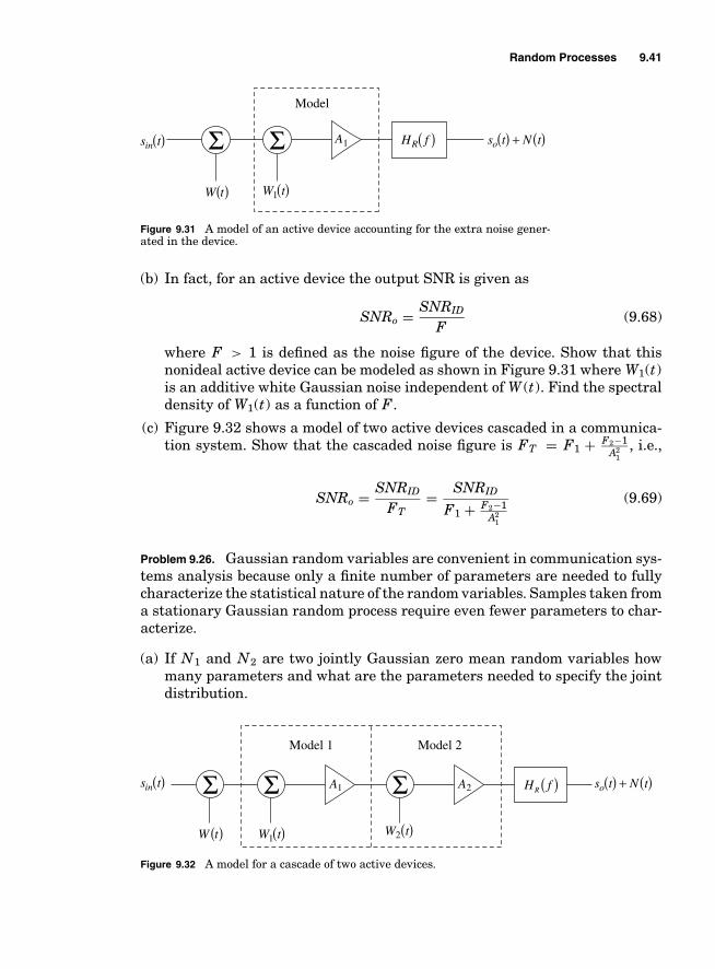
Random Processes 9.41
H fR( )s tin( )
W t( )
A1 s t N to( ) + ( )
W t1( )
Model
ΣΣ
Figure 9.31 A model of an active device accounting for the extra noise gener-ated in the device.
(b) In fact, for an active device the output SNR is given as
SNRo = SNRID
F(9.68)
where F > 1 is defined as the noise figure of the device. Show that thisnonideal active device can be modeled as shown in Figure 9.31 where W1(t)is an additive white Gaussian noise independent of W (t). Find the spectraldensity of W1(t) as a function of F .
(c) Figure 9.32 shows a model of two active devices cascaded in a communica-tion system. Show that the cascaded noise figure is FT = F1 + F2−1
A21
, i.e.,
SNRo = SNRID
FT= SNRID
F1 + F2−1A2
1
(9.69)
Problem 9.26. Gaussian random variables are convenient in communication sys-tems analysis because only a finite number of parameters are needed to fullycharacterize the statistical nature of the random variables. Samples taken froma stationary Gaussian random process require even fewer parameters to char-acterize.
(a) If N1 and N2 are two jointly Gaussian zero mean random variables howmany parameters and what are the parameters needed to specify the jointdistribution.
H fR ( )s tin( )
W t( )
A1 s t N to( ) + ( )
W t1( )
Model 1 Model 2
W t2( )
A2Σ Σ Σ
Figure 9.32 A model for a cascade of two active devices.

9.42 Chapter Nine
(b) If N1 = N (t) and N2 = N (t + τ ) are two jointly Gaussian zero meanrandom variables obtained by sampling a stationary zero mean bandpassGaussian process at time t and t + τ , how many parameters and what arethe parameters needed to specify the joint distribution.
(c) If N1, N2, and N3 are three jointly Gaussian zero mean random variableshow many parameters and what are the parameters needed to specify thejoint distribution.
(d) If N1 = N (t), N2 = N (t + τ ), and N3 = N (t − τ ) are three jointly Gaussianzero mean random variables obtained by sampling a stationary zero meanbandpass Gaussian process at times t, t+τ , and t−τ , how many parametersand what are the parameters needed to specify the joint distribution.
9.8 Example Solutions
Problem 9.4.
(a) Psi = A2
(b) Since the input signal is a DC signal ( f = 0) and has a Fourier transformSi(f ) = Aδ(f ) the output is so(t) = AHR(0). Consequently, Ps = A2|HR(0)|2.
(c)
σ 2N = N0
2
∫ ∞
−∞|HR(f )|2df = N0
2|HR(0)|2
∫ ∞
−∞|HN (f )|2df (9.70)
(d)
SNR = Ps
σ 2N
= 2A2
N0
[∫ ∞
−∞|HN (f )|2 df
]−1
(9.71)
(e) Using the definition of BN gives
BN = 12|HR(0)|2
∫ ∞
−∞|HR(f )|2df = 1
2|HR(0)|2∫ ∞
−∞|HR(0)|2|HN (f )|2df
(9.72)Therefore, BN = 1
2
∫∞−∞ |HN (f )|2 df and SNR = A2
N0 BN.
Problem 9.20.
(a) Note that N1(t) and N2(t) are both zero mean Gaussian processes withcorrelation functions
RNi (τ ) = N0
2
∫ ∞
−∞hi(t)hi(t − τ )dt (9.73)

Random Processes 9.43
Since N (t) = N1(t) + N2(t) and N1(t) is independent of N2(t) we have
σ 2N = RN (0) = var(N (t)) = var(N1(t)) + var(N2(t))
= N0
2
∫ ∞
−∞
(|h1(t)|2 + |h2(t)|2)dt (9.74)
and
fN (t)(n) = 1√2πσ 2
N
exp[− n2
2σ 2N
](9.75)
(b)
P (N (t) > −1) =∫ ∞
−1fN (t)(n)d n = 1
2+ 1
2erf
(1√
2var(N (t))
)(9.76)
(c) Since N (t) is a zero mean process the PDF is characterized with
RN (0) = σ 2N ρN (τ ) = RN (τ )
σ 2N
= N0
2σ 2N
∫ ∞
−∞(h1(t)h1(t − τ ) + h2(t)h2(t − τ ))dt
(9.77)Using these results in
fN (t)N (t−τ )(x, y) = 1
2πσ 2N
√1 − ρ2
N (τ )
× exp
(− 1
2σ 2N
(1 − ρ2
N (τ ))(x2 − 2ρN (τ )xy + y2)) (9.78)
(d) Recall that
fN (t)(x|N (t − τ ) = y) = 1
σN
√2π(1 − ρ2
N (τ ))
× exp
(− 1
2σ 2N
(1 − ρ2
N (τ )) (x − ρN (τ )y)2
)(9.79)
(e) The effective transfer function from input 1 to the output is
HE1(f ) = H1(f )(1 − H3(f )) (9.80)
The effective transfer function from input 2 to the output is
HE2(f ) = −H2(f )H3(f ) (9.81)
Since both of the input noises, Wi(t), are independent the output powerspectrum is given as
SE (f ) = N0
2|H1(f )(1 − H3(f ))|2 + N0
2| − H2(f )H3(f )|2 (9.82)

9.44 Chapter Nine
9.9 Miniprojects
Goal: To give exposure
■ to a small scope engineering design problem in communications.■ to the dynamics of working with a team.■ to the importance of engineering communication skills (in this case oral pre-
sentations).
Presentation: The forum will be similar to a design review at a company(only much shorter). The presentation will be of 5 minutes in length with anoverview of the given problem and solution. The presentation will be followedby questions from the audience (your classmates and the professor). Each teammember should be prepared to give the presentation.
9.9.1 Project 1
Project Goals: To use your engineering knowledge of random processes tosolve a practical engineering problem.
You have a voice signal with average power of −10 dBm and bandwidth of4 kHz that you want to transmit over a cable from one building on campus toanother building on campus. The system block diagram is shown in Figure 9.33.The noise in the receiver electronics is accurately modeled as an AWGN with aone-sided noise spectral density of N0 = −174 dBm/Hz. The cable is accuratelymodeled as a filter with the following impulse response
hc(t) = Lpδ(t − τp) (9.83)
where Lp is the cable loss. You are using cable with a loss of 2 dB/1000 ft. Howlong of a cable can be laid and still achieve at least 10 dB SNR? If the signalwas changed to a video signal with −10 dBm average power and bandwidth of6 MHz, how long of a cable can be laid and still achieve at least 10 dB SNR?
9.9.2 Project 2
Project Goals: To use the knowledge of random process theory to identify thecharacteristics of an electronic signal.
MessageSource
m t( )Channel
Noise
LowpassFilter H( f )
OutputΣ
Figure 9.33 Block diagram of a baseband (cable) communication system.

Random Processes 9.45
You have been given a radio receiver that was recovered from a crash siteof an alien spacecraft and are part of a project team that has been asked tounderstand this radio. The technician on your project has sampled a waveform,N (t), from the radio output at a sample rate of f s = 10 MHz and put it inthe file aliennoise.mat. Examine the file and determine whether you think thesignal can be characterized as Gaussian and/or stationary. If the process is wellmodeled as Gaussian and stationary then estimate the correlation function,RN (τ ), and the power spectral denisty, SN (f ), of this process. Determine whatbandwidth contains 99% of the signal power.

This page intentionally left blank

Chapter
10Noise in Bandpass
Communication Systems
Noise in communication systems is produced from a filtering operation on thewideband noise that appears at the receiver input. Most communication occursin a fairly limited bandwidth around some carrier frequency. Since Chapter 9showed that the input noise in a communication system is well modeled as anadditive white Gaussian noise, it makes sense to limit the effects of this noise byfiltering around this carrier frequency. Consequently, the canonical model fornoise in a bandpass communication system is given in Figure 10.1. The whitenoise, W (t), models a wideband noise which is present at the receiver input.This noise can come from a combination of the receiver electronics, man-madenoise sources, or galactic noise sources. This noise is often well modeled as azero mean, stationary, and Gaussian random process with a power spectraldensity of N0/2 W/Hz. The filter, HR(f ), represents the frequency response ofthe receiver system. This frequency response is often designed to have a band-pass characteristic to match the transmission band and is bandpass aroundthe carrier frequency, f c. Chapter 9 showed that Nc(t) is a stationary Gaussianprocess with a power spectral density (PSD) of
SNc (f ) = |HR(f )|2 N0
2(10.1)
The noise, Nc(t), will consequently have all it’s power concentrated aroundthe carrier frequency, f c. Noise with this characteristic is denoted bandpassnoise. The average power of the noise is given as
E[N 2
c (t)] = σ 2
N =∫ ∞
−∞SNc (f )df = N0
2
∫ ∞
−∞|HR(f )|2df (10.2)
This noise in a bandpass communication system will then be passed throughan I/Q downconverter to produce an in-phase noise, N I (t), and a quadrature
10.1
Copyright © 2007 by The McGraw-Hill Companies. Click here for terms of use.

10.2 Chapter Ten
W t( )
ChannelLpxc(t − τp) Yc(t) = rc(t) + Nc(t)
rI (t) + NI(t)
ts
ts
rQ(t) + NQ(t)
xc(t) HR( f )I/Q
Down-converter
Σ
rI (ts) + NI(ts)
rQ(ts) + NQ(ts)
Figure 10.1 The canonical model for communication system analysis.
noise, N Q(t). This chapter provides the necessary tools to characterize the low-pass noise processes, N I (t) and N Q(t), that result in this situation.
EXAMPLE 10.1Consider a receiver system with an ideal bandpass filter response of bandwidth BTcentered at fc, i.e.,
HR(f ) ={
A || f | − fc| ≤ BT2
0 elsewhere(10.3)
where A is a real, positive constant. The bandpass noise will have a spectral density of
SNc (f ) =
⎧⎨⎩
A2N0
2|| f | − fc| ≤ BT
2
0 elsewhere(10.4)
Consequently
E[N 2
c (t)] = σ 2
N =∫ ∞
−∞SNc (f )df = A2 N0 BT (10.5)
These tools will enable an analysis of the performance of bandpass commu-nication systems in the presence of noise. This ability to analyze the effectsof noise is what distinguishes the competent communication systems engineerfrom the hardware designers and the technicians they work with. The simplestanalysis problem is examining a particular point in time, ts, and character-izing the resulting noise samples, N I (ts) and N Q(ts), to extract a parameterof interest, e.g., average signal-to-noise ratio (SNR). Bandpass communica-tion system performance can be characterized completely if probability densityfunctions (PDF) of the noise samples of interest can be identified, e.g.,
f N I (n1), f N I (t)N I (t+τ )(n1, n2), and/or f N Q(t)N I (t+τ )(n1, n2) (10.6)

Noise in Bandpass Communication Systems 10.3
To accomplish this analysis task this chapter first introduces notation fordiscussing the bandpass noise and the lowpass noise. The resulting lowpassnoise processes are shown to be zero mean, jointly stationary, and jointly Gaus-sian. Consequently, the PDFs like those detailed in Eq. (10.6) will entirely bea function of the second order statistics of the lowpass noise processes. Thesesecond order statistics can be produced from the PSD given in Eq. (10.1).
EXAMPLE 10.2If a sampled white Gaussian noise like that considered in Figure 9.7(b) with a measuredspectrum like that given in Figure 9.14(a) is put through a bandpass filter a bandpassnoise will result. For the case of a bandpass filter with a center frequency of 6500 Hz anda bandwidth of 2000 Hz one sample path of the measured output PSD, SNc ( f , ω1, T m),is shown in Figure 10.2(a). An estimate of the PSD using an average of 4000 samplepaths is shown in Figure 10.2(b). The validity of Eq. (10.1) is clearly evident in thisoutput PSD as this PSD can be viewed as the multiplication of the input white PSD anda bandpass transfer function. One resulting sample function of this output bandpassnoise, Nc(t, ω1) is given in Figure 10.3(a). A histogram of 4000 output samples takenat t = 0.0045 seconds of this noise process, Nc(0.0045), is shown in Figure 10.3(b).This histogram demonstrates that a bandpass noise as is typically seen in bandpasscommunication systems is well modeled as a zero mean Gaussian random process.
Point 1: In bandpass communications the input noise, Nc(t), is a stationaryGaussian random process with power spectral density given in Eq. (10.1).The effect of noise on the performance of a bandpass communication systemcan be analyzed if the PDFs of the noise samples of interest can be charac-terized as in Eq. (10.6).
−1−0.8 −0.6 −0.4 −0.2 0
(a) One sample function fo the measured PSD,SNc
( f, w1, Tm)
0.2 0.4 0.6 0.8 1× 10⁴
−100
−90
−80
−70
−60
−50
−40
−30
Frequency, f, Hz
S NC(f
,w1,
Tm
), d
B
−1 −0.8 −0.6 −0.4 −0.2 0
(b) An estimate of the PSD using a 4000 trialaverage.
0.2 0.4 0.6 0.8 1× 10⁴
−100
−90
−80
−70
−60
−50
−40
−30
Frequency, f, Hz
S NC(f
,w1,
Tm
), d
B
Figure 10.2 The measured spectral characteristics of bandpass filtered white noise.

10.4 Chapter Ten
0.046 0.048 0.050 0.052 0.054−1.5
−1
−0.5
0
0.5
1
1.5
Time, t, sec(a) A sample function
Nc(
t)
−1.5 −1 −0.5 0
(b) A histogram of realizationsof Nc(0.0045), 4000 trials.
0.5 1 1.50
50
100
150
200
250
300
Values of Nc(t)
Num
ber
of O
ccur
renc
es
Figure 10.3 Further characterization of bandpass noise resulting from bandpass filtering a white Gaussian noise.
10.1 Bandpass Random Processes
A bandpass random process will have the same form as a bandpass signal.Consequently, it can be written as
Nc(t) = N I (t)√
2 cos(2π f ct) − N Q(t)√
2 sin(2π f ct) (10.7)
= N A(t)√
2 cos(2π f ct + N P (t)) (10.8)
N I (t) in Eq. (10.7) is normally referred to as the in-phase (I) component ofthe noise and N Q(t) is normally referred to as the quadrature (Q) componentof the bandpass noise. The amplitude of the bandpass noise is N A(t) andthe phase of the bandpass noise is N P (t). As in the deterministic case thetransformation between the two representations are given by
N A(t) =√
N I (t)2 + N Q(t)2 N P (t) = tan−1[
N Q(t)N I (t)
]
and
N I (t) = N A(t) cos(N P (t)) N Q(t) = N A(t) sin(N P (t))
A bandpass random process has sample functions which appear to be asinewave of frequency f c with a slowly varying amplitude and phase. An ex-ample of a bandpass random process is shown in Figure 10.3(a). As in the de-terministic signal case, a method of characterizing a bandpass random processwhich is independent of the carrier frequency is desired. The complex enveloperepresentation provides such a vehicle.
The complex envelope of a bandpass random process is defined as
Nz(t) = N I (t) + j N Q(t) = N A(t) exp[ j N P (t)] (10.9)

Noise in Bandpass Communication Systems 10.5
LPF
LPF
Σ+
π 2 π 2
2 2cos π f tc( )
NI(t) N1(t)
N2(t)
−
NQ(t)
NI(t)
−NQ(t)
Nc(t)2 2cos π f tc( )
Figure 10.4 The transformations between bandpass noise and the baseband components.
The original bandpass random process can be obtained from the complex enve-lope by
Nc(t) =√
2[Nz(t) exp[ j 2π f ct]]
Since the complex exponential is a deterministic function, the complex ran-dom process Nz(t) contains all the randomness in Nc(t). In a similar fashionas a bandpass signal, a bandpass random process can be generated from its Iand Q components and a complex baseband random process can be generatedfrom the bandpass random process. Figure 10.4 shows these transformations.Figure 10.5 shows a bandpass noise and the resulting in-phase and quadra-ture components that are output from a downconverter structure shown inFigure 10.4.
0.046 0.048 0.050 0.052 0.054−1.5
−1
−0.5
0
0.5
1
1.5
Time, t, sec(a) Bandpass noise
Nc(
t)
0.046 0.048 0.050 0.052 0.054−1.5
−1
−0.5
0
0.5
1
1.5
Time, t, sec
NQ(t)
(b) Baseband noises
Noi
se V
alue
NI(t)
Figure 10.5 A bandpass noise and the resulting in-phase and quadrature noises. BT = 2000 Hz and fc = 6500 Hz.

10.6 Chapter Ten
Correlation functions are important in characterizing random processes.Autocorrelation functions were a focus of Chapter 9. For bandpass processesthe crosscorrelation function will be important as well.
Definition 10.1 Given two real random processes, N I (t) and N Q(t), the crosscorrelationfunction between these two random processes is given as
RN I N Q (t1, t2) = E[N I (t1)N Q(t2)] (10.10)
The crosscorrelation function is a measure of how similar the two random pro-cesses behave. In an analogous manner to the discussion in Chapter 9 a cross-correlation coefficient can be defined.
The correlation function of a bandpass random process, which is derived usingEq. (10.7), is given by
RNc (t1, t2) = E[Nc(t1)Nc(t2)]
= 2RN I (t1, t2) cos(2π f ct1) cos(2π f ct2) − 2RN I N Q (t1, t2) cos(2π f ct1)
× sin(2π f ct2) − 2RN Q N I (t1, t2) sin(2π f ct1) cos(2π f ct2)
+ 2RN Q (t1, t2) sin(2π f ct1) sin(2π f ct2) (10.11)
Consequently, the correlation function of the bandpass noise is a function ofboth the correlation function of the two lowpass noise processes and the cross-correlation between the two lowpass noise processes.
Definition 10.2 The correlation function of the complex envelope of a bandpass randomprocess is
RNz(t1, t2) = E[Nz(t1)N ∗z (t2)] (10.12)
Using the definition of the complex envelope given in Eq. (10.9) produces
RNz(t1, t2) = RN I (t1, t2) + RN Q (t1, t2) + j [−RN I N Q (t1, t2) + RN Q N I (t1, t2)](10.13)
The correlation function of the bandpass signal, RNc (t1, t2), is derived from thecomplex envelope, via
RNc (t1, t2) = 2E([Nz(t1) exp[ j 2π f ct1]][N ∗z (t2) exp[− j 2π f ct2]]) (10.14)
This complicated function can be simplified in some practical cases. The casewhen the bandpass random process, Nc(t), is a stationary random process isone of them.
10.2 Characteristics of the Complex Envelope
10.2.1 Three Important Results
This section shows that the lowpass noise, N I (t) and N Q(t) derived from abandpass noise, Nc(t), are zero mean, jointly Gaussian, and jointly station-ary when Nc(t) is zero mean, Gaussian, and stationary. These characteristics

Noise in Bandpass Communication Systems 10.7
simplify the description of N I (t) and N Q(t) considerably. Important quantitiesin this analysis will be
N1(t) = Nc(t)√
2 cos(2π f ct)
N2(t) = −Nc(t)√
2 sin(2π f ct) (10.15)
which are the outputs of the multipliers in the down converter in Figure 10.4.
Property 10.1 If the bandpass noise, Nc(t), has a zero mean, then N I (t) and N Q(t) bothhave a zero mean.
Proof: This property’s validity can be proved by considering how N I (t) (orN Q(t)) is generated from Nc(t) as shown in Figure 10.4. The I component ofthe noise is expressed as
N I (t) = N1(t) ∗ hL(t) =√
2∫ ∞
−∞hL(t − τ )Nc(τ ) cos(2π f cτ )dτ
where hL(t) is the impulse response of the lowpass filter. Neither hL(t) nor thecosine term are random, so the linearity property of the expectation operatorcan be used to obtain
E(N I (t)) =√
2∫ ∞
−∞hL(t − τ )E(Nc(τ )) cos(2π f cτ )dτ = 0
The same ideas holds for N Q(t). �
This property is important since the input thermal noise to a communicationsystem is typically zero mean; consequently, the I and Q components of theresulting bandpass noise will also be zero mean.
Definition 10.3 Two random processes N I (t) and N Q(t) are jointly Gaussian randomprocesses if any set of samples taken from the two processes are a set of joint Gaussianrandom variables.
Property 10.2 If the bandpass noise, Nc(t), is a Gaussian random process then N I (t)and N Q(t) are jointly Gaussian random processes.
Proof: The detailed proof techniques are beyond the scope of this course but arecontained in most advanced texts concerning random processes (e.g., [DR87]).A sketch of the ideas needed in the proof is given here. A random process whichis a product of a deterministic waveform and a Gaussian random process isstill a Gaussian random process. Hence N1(t) and N2(t) are jointly Gaussianrandom processes. N I (t) and N Q(t) are also jointly Gaussian processes sincethey are linear functionals of N1(t) and N2(t) (i.e., N I (t) = N1(t) ∗hL(t)). �
Again this property implies that the I and Q components of the bandpassnoise in most communication systems will be well modeled as Gaussian ran-dom processes. It is easy to deduce that many of the samples of N I (t) (and sim-ilarly N Q(t)) are Gaussian random variables. Sampling Nc(t) at t = k/(2 f c)where k is an integer gives Nc(k/(2 f c)) = (−1)k N I (k/(2 f c)). Since Nc(t) is a

10.8 Chapter Ten
−1.5 −1 −0.5 0
(a) NI (0.045)
0.5 1 1.50
50
100
150
200
250
300
Values of NI(t)
Num
ber
of O
ccur
renc
es
−1.5 −1 −0.5 0
(b) NQ(0.045)
0.5 1 1.50
50
100
150
200
250
300
Values of NQ(t)
Num
ber
of O
ccur
renc
esFigure 10.6 Histogram of samples of the random variables N I (0.045) and N Q(0.045) after downconverting a band-pass noise process.
Gaussian random process these samples are Gaussian random variables andconsequently many samples of the lowpass processes are also Gaussian randomvariables. Property 10.2 simply implies that all jointly considered samples ofN I (t) and N Q(t) are jointly Gaussian random variables.
EXAMPLE 10.3Consider the previous bandpass filtered noise example where fc = 6500 Hz and thebandwidth is 2000 Hz. Figure 10.6 shows histogram of samples of the random variableN I (0.045) and N Q(0.045) (i.e., the lowpass processes sampled at t = 45 ms) after down-conversion of a bandpass noise process. Again it is apparent from this figure that thelowpass noise is well modeled as a zero mean Gaussian random process. It is interestingto note that at least in this example samples from N I (t) and N Q(t) appear to have acommon distribution.
Property 10.3 If a bandpass signal, Nc(t), is a stationary Gaussian random process,then N I (t) and N Q(t) are also jointly stationary, jointly Gaussian random processes.
Proof: Define the random process Nz1(t) = N1(t) + j N2(t) = Nc(t)√
2 ×exp[− j 2π f ct]. Since Nc(t) is a stationary Gaussian random process thenRNz1 (t1, t2) = 2RNc (τ ) exp[− j 2π f cτ ] = RNz1 (τ ) where τ = t1 − t2. Since Nz(t) =Nz1(t) ∗hL(t), if Nz1(t) is stationary then the stationarity of the output complexenvelope, Nz(t), is due to Property 9.11. Using the stationarity of Nz(t) withthe result in Eq. (10.13) gives the following relationship
RNz(τ ) = RN I (t1, t2)+RN Q (t1, t2)+ j[−RN I N Q (t1, t2)+RN Q N I (t1, t2)
](10.16)

Noise in Bandpass Communication Systems 10.9
which implies that both the real and imaginary part of RNz(τ ) must only befunctions of τ so that
RN I (t1, t2) + RN Q (t1, t2) = g1(τ ) − RN I N Q (t1, t2) + RN Q N I (t1, t2) = g2(τ )(10.17)
Alternately, since Nc(t) has the form given in Eq. (10.11) a rearrangement(by using trigonometric identities) with t2 = t1 − τ gives
RNc (τ ) = [RN I (t1, t2) + RN Q (t1, t2)]
cos(2π f cτ ) + [RN I (t1, t2) − RN Q (t1, t2)]
× cos(2π f c(2t2 + τ )) + [RN I N Q (t1, t2) − RN Q N I (t1, t2)]
sin(2π f cτ )
−[RN I N Q (t1, t2) + RN Q N I (t1, t2)]
sin(2π f c(2t2 + τ )) (10.18)
Since Nc(t) is Gaussian and stationary this implies that the right-hand sideof Eq. (10.18) is a function only of the time difference, τ and not the absolutetime t2. Consequently, the factors multiplying the sinusoidal terms having ar-guments containing t2 must be zero. Consequently, a second set of constraintsis
RN I (t1, t2) = RN Q (t1, t2) RN I N Q (t1, t2) = −RN Q N I (t1, t2) (10.19)
The only way for Eq. (10.17) and Eq. (10.19) to be satisfied is if
RN I (t1, t2) = RN Q (t1, t2) = RN I (τ ) = RN Q (τ ) (10.20)
RN I N Q (t1, t2) = −RN Q N I (t1, t2) = RN I N Q (τ ) = −RN Q N I (τ ) (10.21)
Since all correlation functions and crosscorrelation functions are functions of τ
then N I (t) and N Q(t) are jointly stationary. �
Point 2: If the input noise, Nc(t), is a zero mean, stationary, Gaussian ran-dom process then N I (t) and N Q(t) are zero mean, jointly Gaussian, andjointly stationary.
10.2.2 Important Corollaries
This section discusses several important corollaries to the important resultsderived in the last section. The important result from the last section is sum-marized as follows: if Nc(t) is zero mean, Gaussian and stationary then N I (t)and N Q(t) are zero mean, jointly Gaussian, and jointly stationary.
Property 10.4
RN I (τ ) = RN Q (τ ) (10.22)
Surprisingly, this property, given in Eq. (10.20), implies that both N I (t) andN Q(t) behave in a statistically identical manner. Consequently, the power ofthe noise in each component is identical, i.e., E[N 2
I (t)] = E[N 2Q(t)] = σ 2
N I. This
is empirically confirmed by examining the histograms in Figure 10.6.

10.10 Chapter Ten
Property 10.5
RN I N Q (τ ) = −RN I N Q (−τ ) (10.23)
This property, due to Eq. (10.21), implies RN I N Q (τ ) is an odd function withrespect to τ .
Property 10.6 RNz(τ ) = 2RN I (τ ) − j 2RN I N Q (τ )
Proof: This is shown by using Eq. (10.22) and Eq. (10.23) in Eq. (10.13). �
This implies that the real part of RNz(τ ) is an even function of τ and theimaginary part of RNz(τ ) is an odd function of τ .
Property 10.7
RNc (τ ) = 2RN I (τ ) cos(2π fcτ ) + 2RN I N Q (τ ) sin(2π fcτ ) = [RNz(τ ) exp( j 2π fcτ )]
(10.24)
Proof: This is shown by using Eq. (10.22) and Eq. (10.23) in Eq. (10.18). �
This property implies there is a simple relationship between the correlationfunction of the stationary Gaussian bandpass noise and the correlation functionof the complex envelope of the bandpass noise. This relationship has significantparallels to the relationship between bandpass and the baseband signals givenin Chapter 4.
Property 10.8 var(Nc(t)) = σ 2N = var(N I (t)) + var(N Q(t)) = 2var(N I (t)) = var(Nz(t))
= 2σ 2N I
Proof: This is shown by using Eq. (10.22) in Eq. (10.24) for τ = 0. �
This property states that the power in the bandpass noise is the same asthe power in the complex envelope. This power in the bandpass noise is alsothe sum of the powers in the two lowpass noises which comprise the complexenvelope.
Property 10.9 For the canonical problem considered in this chapter, N I (t) and N Q(t)are completely characterized by the functions RN I (τ ) and RN I N Q (τ ).
Proof: Any joint PDF of samples taken from jointly stationary and jointlyGaussian processes are completely characterized by the first- and second-ordermoments. Note, first that N I (t) and N Q(t) are zero mean processes. Conse-quently, the characterization of the process only requires the identification ofthe variance, σ 2
N I= RN I (0), and the correlation coefficient between samples.
The correlation coefficient between samples from the same process is givenas ρN I (τ ) = RN I (τ )/RN I (0) while the correlation coefficient between samplestaken from N I (t) and N Q(t) is ρN I N Q (τ ) = RN I N Q (τ )/RN I (0). �

Noise in Bandpass Communication Systems 10.11
EXAMPLE 10.4If one sample from the in-phase noise is considered then
f N I (ni) = 1√2πσ 2
N I
exp
(− n2
i
2σ 2N I
)(10.25)
where σ 2N I
= RN I (0).
EXAMPLE 10.5If two samples from the in-phase noise are considered then
f N I (t)N I (t−τ )(n1, n2) = 1
2πσ 2N I
√(1 − ρ2
N I(τ )) exp
[−(n2
1 − 2ρN I (τ )n1n2 + n22
)2σ 2
N I
(1 − ρ2
N I(τ ))]
where ρN I (τ ) = RN I (τ )/RN I (0).
EXAMPLE 10.6If one sample each from the in-phase noise and the quadrature noise are consideredthen
f N I (t)N Q(t−τ )(n1, n2) = 1
2πσ 2N I
√(1 − ρ2
N I N Q(τ )) exp
[−(n2
1 − 2ρN I N Q (τ )n1n2 + n22
)2σ 2
N I
(1 − ρ2
N I N Q(τ ))]
where ρN I N Q (τ ) = RN I N Q (τ )/√
RN I (0)RN Q (0) = RN I N Q (τ )/RN I (0).
Property 10.10 The random variables N I (ts) and N Q(ts) are independent random vari-ables for any value of ts.
Proof: From Eq. (10.23) we know RN I N Q (τ ) is an odd function. Consequently,RN I N Q (0) = 0. Since N I (t) and N Q(t) are jointly Gaussian and orthogonal ran-dom variables then they are also independent. �
Any joint PDF of samples of N I (ts) and N Q(ts) taken at the same time have thesimple PDF
f N I (t)N Q(t)(n1, n2) = 12πσ 2
N I
exp
[−(n2
1 + n22
)2σ 2
N I
](10.26)
This simple PDF will prove useful in our performance analysis of bandpasscommunication systems.

10.12 Chapter Ten
Point 3: Since N I (t) and N Q(t) are zero mean, jointly Gaussian, and jointlystationary then a complete statistical description of N I (t) and N Q(t) is avail-able from RN I (τ ) and RN I N Q (τ ).
10.3 Spectral Characteristics
At this point we need a methodology to translate the known PSD of the band-pass noise Eq. (10.1) into the required correlation function, RN I (τ ), and therequired crosscorrelation function, RN I N Q (τ ). To accomplish this goal we needa definition.
Definition 10.4 For two random processes N I (t) and N Q(t) whose crosscorrelation func-tion is given as RN I N Q (τ ) the cross spectral density is
SN I N Q (f ) = F{
RN I N Q (τ )}
(10.27)
Property 10.11 The PSD of Nz(t) is given by
SNz(f ) = F{
RNz(τ )} = 2SN I (f ) − j 2SN I N Q (f ) (10.28)
where SN I (f ) and SN I N Q (f ) are the power spectrum of N I (t) and the crosspower spec-trum of N I (t) and N Q(t), respectively.
Proof: This is seen taking the Fourier transform of RNz(τ ) as given in Prop-erty 10.6. �
Property 10.12 SN I N Q (f ) is purely an imaginary function and an odd function of f .
Proof: This is true since RN I N Q (τ ) is an odd real valued function (see Prop-erty 2.6). A power spectral density must be real and positive so by examiningEq. (10.28) it is clear SN I N Q (f ) must be imaginary for SNz(f ) to be a valid powerspectral density. �
Property 10.13 The even part of SNz(f ) is due to SN I (f ) and the odd part is due toSN I N Q (f ).
Proof: A spectral density of a real random process is always even. SN I (f ) isa spectral density of a real random process. By Property 10.12, SN I N Q (f ) is apurely imaginary and odd function of frequency. �
Property 10.14
SN I (f ) = SNz(f ) + SNz(− f )4
SN I N Q (f ) = SNz(− f ) − SNz(f )j 4
Proof: This is a trivial result of Property 10.13 �
Consequently, Property 10.14 provides a simple method to compute SN I (f ) andSN I N Q (f ) once SNz(f ) is known. SNz(f ) can be computed from SNc (f ) given inEq. (10.1) in a simple way as well.

Noise in Bandpass Communication Systems 10.13
Property 10.15
SNc (f ) = 12
SNz( f − fc) + 12
SNz(− f − fc)
Proof: Examining Eq. (10.24) and the frequency translation theorem of theFourier transform, the spectral density of the bandpass noise, Nz(t), is ex-pressed as
SNc (f ) = 2SN I (f ) ∗[
12
δ( f − f c) + 12
δ( f + f c)]
+ 2SN I N Q (f ) ∗[
12 j
δ( f − f c) − 12 j
δ( f + f c)]
where ∗ again denotes convolution. This equation can be rearranged to give
SNc (f ) = [SN I ( f − f c) − j SN I N Q ( f − f c)]+ [SN I ( f + f c) + j SN I N Q ( f + f c)
](10.29)
Noting that due to Property 10.12
SNz(− f ) = 2SN I (f ) + j 2SN I N Q (f ) (10.30)
Equation (10.29) reduces to the result in Property 10.15. �
This is a very fundamental result. Property 10.15 states that the power spec-trum of a bandpass random process is simply derived from the power spectrumof the complex envelope and vice versa. For positive values of f , SNc (f ) is ob-tained by translating SNz(f ) to f c and scaling the amplitude by 0.5 and fornegative values of f , SNc (f ) is obtained by flipping SNz(f ) around the ori-gin, translating the result to − f c, and scaling the amplitude by 0.5. LikewiseSNz(f ) is obtained from SNc (f ) by taking the positive frequency PSD which iscentered at f c and translating it to baseband ( f = 0) and multiplying it by 2.Property 10.15 also demonstrates in another manner that the average power ofthe bandpass and baseband noises are identical since the area under the PSDis the same (this was previously shown in Property 10.8).
EXAMPLE 10.7Example 10.1 showed a receiver system with an ideal bandpass filter that had a band-pass noise PSD of
SNc (f ) ={
A2 N02 || f | − fc| ≤ BT
2
0 elsewhere(10.31)
Moving the positive frequency portion of the spectrum at fc to baseband and doublingthe height gives
SNz(f ) ={
A2N0 | f | ≤ BT2
0 elsewhere(10.32)

10.14 Chapter Ten
−1−0.8 −0.6 −0.4 −0.2 0
(a) One sample path
0.2 0.4 0.6 0.8 1× 104 × 104
−100
−90
−80
−70
−60
−50
−40
−30
Frequency, f, Hz
S NZ(f
,w1,
Tm
), d
B
−1−0.8 −0.6 −0.4 −0.2 0
(b) Average of 4000 sample paths
0.2 0.4 0.6 0.8 1−100
−90
−80
−70
−60
−50
−40
−30
Frequency, f, Hz
S NZ(f
,w1,
Tm
), d
BFigure 10.7 The measured PSD of the complex envelope of a bandpass process resulting from bandpass filtering awhite noise.
Since there is no odd part to this PSD
SN I (f ) ={
A2 N02 | f | ≤ BT
2
0 elsewhereSN I N Q (f ) = 0 � (10.33)
Again considering the previous example of bandpass filtered white noise with fc =6500 Hz and a bandwidth of 2000 Hz a resulting measured power spectral density of thecomplex envelope is given in Figure 10.7. This measured PSD demonstrates the validityof the analytical results given in Eq. (10.36).
EXAMPLE 10.8Consider an example PSD that might appear in a receiver for SSB-AM transmissiongiven as
SNc (f ) ={
A2 N02 0 ≤ | f | − fc ≤ BT
0 elsewhere(10.34)
Moving the positive frequency portion of the spectrum at fc to baseband and doublingthe height gives
SNz(f ) ={
A2N0 0 ≤ f ≤ BT
0 elsewhere(10.35)

Noise in Bandpass Communication Systems 10.15
Finding the even and odd parts of this PSD using Property 10.14 gives
SN I (f ) ={
A2 N04 | f | ≤ BT
0 elsewhereSN I N Q (f ) =
⎧⎪⎪⎪⎨⎪⎪⎪⎩
A2 N0j 4 −BT ≤ f ≤ 0
−A2 N0j 4 0 ≤ f ≤ BT
0 elsewhere(10.36)
It is clear from this example that the random processes N I (t) and N Q(t) are in some waycorrelated. The exact correlation can be computed by an inverse Fourier transform. Theother interesting characteristic resulting from this example is that the same bandpassnoise spectrum resulted in significantly different baseband noise characteristics depen-dent on the selected value of fc in the downconverter. As one example of the differentcharacteristics, the baseband noise in this example has twice the bandwidth of the noisein the previous example while the bandpass noise in each case had the same bandwidth.
Point 4: SN I (f ) and SN I N Q (f ) can be computed in a straightforward fashionfrom SNc (f ) given in Eq. (10.1). An inverse Fourier transform will producethe functions RN I (τ ) and RN I N Q (τ ). From RN I (τ ) and RN I N Q (τ ) a completestatistical description of the complex envelope noise process can be obtained.
10.4 The Solution of the Canonical Bandpass Problem
The tools and results are now in place to completely characterize the complexenvelope of the bandpass noise typically encountered in a bandpass communi-cation system. First, the characterization of one sample, N I (ts), of the randomprocess N I (t) is considered (or equivalently N Q(ts)). This case requires a sixstep process summarized as
1. Identify N0 and HR(f ).
2. Compute SNc (f ) = N02 |HR(f )|2.
3. Compute SNz(f ).
4. Compute
SN I (f ) = SNz(f ) + SNz(− f )4
5. σ 2N I
= RN I (0) = ∫∞−∞ SN I (f )df
6. f N I (ts)(n1) = 1√2πσ 2
N I
exp(
− n21
2σ 2N I
)= f N Q(ts)(n1)
The only difference between this process and the process used for lowpassprocesses as highlighted in Section 9.6 is steps 3–4. These two steps simply arethe transformation of the bandpass PSD into the PSD for one channel of thelowpass complex envelope noise.

10.16 Chapter Ten
EXAMPLE 10.9The previous examples showed a receiver system with an ideal bandpass filter had afterthe completion of steps 1–4
SN I (f ) ={
A2 N02 | f | ≤ BT
2
0 elsewhere(10.37)
Consequently, σ 2N I
= RN I (0) = A2 N0 BT2 .
Second, the characterization of two samples from one of the channels of thecomplex envelope, N I (t1) and N I (t2), is considered. This case requires a sevenstep process summarized as
1. Identify N0 and HR(f ).
2. Compute SNc (f ) = N02 |HR(f )|2.
3. Compute SNz(f ).
4. Compute
SN I (f ) = SNz(f ) + SNz(− f )4
5. RN I (τ ) = F−1{SN I (f )}6. σ 2
N I= RN I (0) and ρN I (τ ) = RN I (τ )/σ 2
N I
7. f N I (t1)N I (t2)(n1, n2) = 12πσ 2
N I
√(1−ρ2
N I(τ ))
exp[
−12σ 2
N I(1−ρ2
N I(τ ))
(n2
1 − 2ρN I (τ )n1n2 + n22
)]
The only difference between this process and the process used for lowpassprocesses as highlighted in Section 9.6 is step 3–4. These two steps again arethe transformation of the bandpass PSD into the PSD for one channel of thelowpass complex envelope noise.
EXAMPLE 10.10The previous examples showed a receiver system with an ideal bandpass filter had afterthe completion of steps 1–4
SN I (f ) ={
A2 N02 | f | ≤ BT
2
0 elsewhere(10.38)
Consequently, step 5 gives σ 2N I
= RN I (0) = A2 N0 BT2 and RN I (τ ) = A2 N0 BT
2 sinc(BT τ ).This implies that ρN I (τ ) = sinc(BT τ ).

Noise in Bandpass Communication Systems 10.17
Finally, the characterization of two samples one from each of the channelsof the complex envelope, N I (t1) and N Q(t2), is considered. This case requires aseven step process summarized as
1. Identify N0 and HR(f ).
2. Compute SNc (f ) = N02 |HR(f )|2.
3. Compute SNz(f ).
4. Compute
SN I (f ) = SNz(f ) + SNz(− f )4
SN I N Q (f ) = SNz(− f ) − SNz(f )j 4
5. RN I N Q (τ ) = F−1{
SN I N Q (f )}
6. σ 2N I
= RN I (0) and ρN I N Q (τ ) = RN I N Q (τ )/σ 2N I
7.f N I (t1)N Q(t2)(n1, n2) = 1
2πσ 2N I
√(1 − ρ2
N I N Q(τ ))
× exp
[−1
2σ 2N I
(1 − ρ2
N I N Q(τ ))(n2
1 − 2ρN I N Q (τ )n1n2 + n22
)]
The only difference between this process and the process for two samples fromthe same channel is the computation of the crosscorrelation function, RN I N Q (τ ).
EXAMPLE 10.11The previous examples showed a receiver system with an ideal bandpass filter had afterthe completion of steps 1–4
SN I (f ) ={
A2 N02 | f | ≤ BT
2
0 elsewhereSN I N Q (f ) = 0 (10.39)
Consequently, step 5 gives σ 2N I
= RN I (0) = A2 N0 BT2 and RN I N Q (τ ) = 0. This implies
that N I (t1) and N Q(t2) are independent random variables regardless of the values of t1and t2.
Similarly, three or more samples from either channel of the complex envelopecould be characterized in a very similar fashion. The tools developed in thischapter give a student the ability to analyze many of the important propertiesof noise that are of interest in a bandpass communication system design.

10.18 Chapter Ten
10.5 Complex Additive White Gaussian Noise
A complex additive white Gaussian noise can be used to accurately model band-pass noise in communication systems. Consider a bandpass noise generated byan ideal bandpass filter, e.g.,
HR(f ) ={
1 f c − Bi ≤ | f | ≤ f c + Bi
0 elsewhere(10.40)
The baseband (complex envelope) power spectrum of the bandpass noise, SNz(f ),and signal will look like that in Figure 10.8(a). Since it is, in general, difficultto build a filter at a carrier frequency that is spectrally compact, the noise spec-trum will typically be wider than the signal spectrum. The baseband processingwill normally cut the noise bandwidth down to something close to W . A “white”noise that has the PSD as given in Figure 10.8(b) will have the exact sameoutput noise characteristics after baseband processing because
1. the baseband processing will only pass the noise in the message bandwidth,W , and
2. the bandpass noise has a complex envelope that has a PSD that is constant,like the white noise, over this band.
Consequently, an accurate model for noise in a bandpass communicationsystem is given as
Yz(t) = rz(t) + Wz(t) (10.41)
where rz(t) is the received signal and Wz(t) is the model for the corrupting noisewhere
SWz(f ) = N0 RWz(τ ) = N0δ(τ ) (10.42)
This model will be denoted complex additive white Gaussian noise in the sequel.A complex AWGN is intended to model a bandpass noise whose bandwidth
is larger than the received signal bandwidth. The advantage of the complex
W(a) Signal and bandpass noise spectra
BR f
SNz( f)
Grz( f)
N0
W(b) Signal and complex white noise spectra
BR f
SNz( f)
Grz( f)
N0
Figure 10.8 Exact and model power spectral densities.

Noise in Bandpass Communication Systems 10.19
AWGN model is that the analysis and algorithm development can proceed ina much cleaner fashion than with a more realistic noise model while not in-trodcing significant modeling errors. This model will be used exclusively in thesequel and the accuracy of the approximation will be explored in the homework.
10.6 Conclusion
Bandpass communication systems will be corrupted by bandpass noise. Thischapter shows that the bandpass noise can be represented with a basebandcomplex noise. This baseband noise is in many cases of interest a zero mean,Gaussian, and stationary random process. A method to completely characterizea bandpass noise was presented. A simplified model for bandpass noise that willbe frequently used in the sequel was also presented. With these tools in place itis now possible to evaluate the resultant message signal reconstruction fidelityof the various demodulation structures that have been proposed.
10.7 Homework Problems
Problem 10.1. What conditions on the bandpass filter characteristic of thereceiver, HR(f ), must be satisfied such that N I (t1) and N Q(t2) are indepen-dent random variables for all t1 and t2 when the input is AWGN?
Problem 10.2. This problem considers noise that might be seen in a vestigialsideband demodulator. Consider a bandpass stationary Gaussian noise at theinput to a demodulator with a spectrum given as
SNc (f ) ={
2 f c − 1000 ≤ | f | ≤ f c + 3000
0 elsewhere(10.43)
Assume operation is in a 1-� system.
(a) What bandpass filter, HR(f ), would produce this spectrum from a whitenoise input with a two-sided noise spectral density of N0/2 = 0.5?
(b) What is the spectral density of N I (t)?
(c) What is E[N 2I (t)]?
(d) Give the joint PDF of N I (t0) and N Q(t0) in a 1-� system for a fixed t0.
(e) Compute SN I N Q (f ).
Problem 10.3. This problem considers noise which might be seen in a single side-band demodulator. Consider a bandpass stationary Gaussian noise at the inputto a demodulator with a spectrum given as
SNc (f ) ={
3.92 × 10⁻³ f c ≤ | f | ≤ f c + 3000
0 elsewhere(10.44)

10.20 Chapter Ten
Assume operation is in a 1-� system.
(a) What is the spectral density of N I (t)?
(b) What is E[N 2I (t)]?
(c) Give the joint PDF of N I (t0) and N Q(t0).
(d) Give the joint PDF of N I (t1) and N Q(t1 − τ ).
(e) Plot the PDF in (d) for τ = 0.0001 and τ = 0.001.
Problem 10.4. Consider a bandpass stationary Gaussian noise at the input to ademodulator with a spectrum given as
SNc (f ) ={
0.001 f c − 2000 ≤ | f | ≤ f c + 2000
0 elsewhere(10.45)
Assume operation is in a 1-� system.
(a) Find and plot the joint density function of N I (t0) and N Q(t0), f N I (t0)N Q(t0)(ni, nq).
(b) Consider the complex random variable Nz(t0) = N I (t0)+ j N Q(t0) = Nz(t0) ×exp(− j φp) and find a one–to–one mapping such that
N I (t0) = g1(N I (t0), N Q(t0)) N Q(t0) = g2(N I (t0), N Q(t0)) (10.46)
(c) Detail the inverse mapping
N I (t0) = h1(N I (t0), N Q(t0)) N Q(t0) = h2(N I (t0), N Q(t0)) (10.47)
(d) Using the results of Section 3.3.4 show that f N I (t0)N Q(t0)(ni,nq) = fN I (t0)N Q(t0)×(ni, nq). In other words, the noise distribution is unchanged by a phaserotation. This result is very important for the study of coherent receiverperformance in the presence of noise detailed in the sequel.
Problem 10.5. Show for a stationary Gaussian bandpass noise, Nc(t), that|SN I N Q (f )| ≤ SN I (f ). If |SN I N Q ( f 0)| = SN I ( f 0) for some f 0 then this places aconstraint on either HR( f c + f 0) or HR( f c − f 0). What is this constraint?
Problem 10.6. For a stationary bandpass noise with complex envelope Nz(t) =N I (t) + j N Q(t) that has a baseband autocorrelation function of RN I (τ ) and abaseband crosscorrelation function of RN I N Q (τ )
(a) Find E[|Nz(t)|2].
(b) Find E[N 2z (t)].
(c) Find E[Nz(t)N ∗z (t − τ )].
(d) Find E[Nz(t)Nz(t − τ )].

Noise in Bandpass Communication Systems 10.21
π/2
LPF
LPF
W(t) HR ( f )
−NQ (t)
Nc (t) 2 cos(2p fct)
NI (t)
Figure 10.9 Noise and the receiver frontend processor.
Problem 10.7. Given the block diagram in Figure 10.9 where W (t) is an AWGNwith two-sided spectral density N0/2 and HR(f ) is a bandpass filter with apassband including f c, find the conditions on the filter HR(f ) such that
(a) N I (t) and N Q(t) have the same correlation function.
(b) RN I (τ ) = RN Q (τ ) = sin(π Bτ )π Bτ
and RN I N Q (τ ) = 0.
Problem 10.8. Real valued additive white Gaussian noise, W (t), with a one-sidedspectral density N0 = 0.01 is input into a bandpass receiver which has a blockdiagram shown in Figure 10.9. The noise power spectrum output from the downconverter is measured as
SNz(f ) ={
0.25 | f | ≤ 100
0 elsewhere(10.48)
(a) Find E[|Nz(t)|2].
(b) Find SN I (f ) and SN I N Q (f ).
(c) What is |HR(f )|?(d) Give the probability density function of one sample of N I (t), i.e., f N I (t)(n).
(e) Compute P (N I (t) > 4).
Problem 10.9. Real valued additive white Gaussian noise, W (t), with a two-sided spectral density N0/2 is input into a demodulator for signal sidebandamplitude modulation which has a block diagram shown in Figure 10.11.The time-invariant filter has a transfer function of
HR(f ) ={
2 f c ≤ | f | ≤ f c + W
0 elsewhere(10.49)
(a) Find the power spectral density of Nc(t), SNc (f )?
(b) Find SN I (f )?

10.22 Chapter Ten
π/2W(t) HR ( f )
H1( f )
H2( f ) NQ (t)
Nc (t) 2 cos(2π fct)
NI (t)~
~
Figure 10.10 A bandpass noise model.
(c) Calculate RN I (τ ).
(d) Detail out the form for the probability density function (PDF) of one samplefrom N I (t), f N I (ts)(n).
(e) Find SN I N Q (f ).
(f) Find the joint PDF of samples taken from N I (t) and N Q(t) taken at thesame time, f N I (ts)N Q(ts)(ni, nq).
Problem 10.10. Consider the model given in Figure 10.10 where W (t) is a realAWGN with one–sided power spectral density of N0. H1(f ) and H2(f ) are twopotentially different filters. This problem investigates how the characteristicsof the bandpass noise change if the filter in the I channel is different from thefilter in the Q channel.
(a) Find the power spectral density of N I (t), SN I(f ), in terms of SN I (f ).
(b) Show that
RN I N Q(τ ) =
∫ ∞
−∞h(λ1)∫ ∞
−∞RN I N Q (τ + λ2 − λ1)h2(λ2)dλ2dλ1 (10.50)
(c) Show that
SN I N Q(f ) = SN I N Q (f )H ∗
2 (f )H1(f ) (10.51)
(d) Will N I (t) always be independent of N Q(t) as when the filters are the same?If not then give an example?
(e) Give conditions on H1(f ) and H2(f ) such that SN I N Q(f ) would be imaginary
and odd as is the case for SN I N Q (f ). If these conditions were satisfied wouldN I (t) always be independent of N Q(t)?
Problem 10.11. Show that if Nz(t) is a stationary complex envelope of a bandpassnoise and Nz(t) = Nz(t) exp[ j φp] then
(a) RN I(τ ) = RN Q
(τ ) = RN I (τ )
(b) RN I N Q(τ ) = RN I N Q (τ )
Problem 10.12. Real valued additive white Gaussian noise, W (t), with a two-sidedspectral density N0/2 is input into a demodulator which has a block diagram

Noise in Bandpass Communication Systems 10.23
W(t) HR ( f )
HL ( f )NQ (t)
NL (t)
Nc (t) I/QDown-
converter
NI (t)
Figure 10.11 Demodulator block diagram.
shown in Figure 10.11. The time-invariant filter has a transfer function of
HR(f ) ={
2 f c − 100 ≤ | f | ≤ f c + 100
0 elsewhere(10.52)
(a) Find the power spectral density of Nc(t), SNc (f ).
(b) E[N 2c (t)] = 2, what is N0?
(c) Find the power spectral density of N I (t), SN I (f ) when E[N 2c (t)] = 2.
(d) Find E[N 2I (t)] for the value of N0 obtained in (b).
(e) Assume that HL(f ) is an ideal lowpass filter with HL(0) = 1. Choose thebandwidth of the filter such that E[N 2
L(t)] = 12 E[N 2
I (t)].
Problem 10.13. An interesting relationship exists between the power spectraldensity of a phase noise and the distribution of the instanteous frequency de-viation. This problem explores this relationship, which has proven useful inpractice, using the techniques introduced in this chapter and in the develop-ment of angle modulation. Assume a random process is characterized as
Nz(t) = Ac exp[ j N p(t)] (10.53)
where N p(t) is a phase noise generated in, for example, a frequency synthesizer.
(a) Show that
RNz(t, τ ) = E[Nz(t)N ∗z (t − τ )] ≈ A2
c E[exp( j 2π Fd (t)τ )] (10.54)
where Fd (t) = 12π
dd t N p(t).
(b) If Fd (t) is a stationary random process, show that
RNz(t, τ ) ≈ RNz(τ ) ≈ A2c�Fd (τ ) (10.55)
where �Fd (t) is the characteristic function1 of a sample of the random pro-cess Fd (t).
1The characteristic function of a random variable was introduced in Problem 3.24 in this textbut is a common tool in the analysis of noise [LG89, Hel91].

10.24 Chapter Ten
m(t)Yz(t) = xz(t) exp( jfp) + Nz(t)Vz(t) = xz(t) + Nz(t)
HL( f )
exp(−jfp)
~
ˆ
Figure 10.12 A demodulator block diagram.
(c) Finally show that
SNz(f ) ≈ A2c f Fd (f ) (10.56)
where f Fd (f ) is the PDF of the random variable Fd (t).
(d) Make an engineering assessment of the validity and the shortcomings ofthe approximations in this problem.
Problem 10.14. It is clear from Example 10.7 and Example 10.8 that a basebandnoise of varying bandwidth can be produced depending on the f c that is chosenin the downconverter. For reasonable choices of f c what are the maximumand minimum bandwidths that a lowpass noise process would possess for abandpass bandwidth of BT .
Problem 10.15. In a DSB-AM receiver modeled with Figure 10.12, the followingcomplex envelope is received
Yz(t) = cos(200πt) exp[ j φp] + Nz(t) (10.57)
Assume m(t) = me(t) + N I (t) and for simplicity that the bandpass noise, Nz(t)is characterized as a white noise
SNz(f ) = N0 (10.58)
The lowpass filter has a transfer function of
HL(f ) = 11 + j f
f l
(10.59)
(a) Prove N I (t) is a stationary random process.
(b) Compute me(t) (the signal at the filter output).
(c) Compute E[N 2I (t)] as a function of f l. Hint: Power can be computed in the
time and frequency domain.
(d) Compute the output SNR as a function of f l.
(e) What value of f l optimizes the output SNR?

Noise in Bandpass Communication Systems 10.25
220200180−220 −200 −180 f
SNc(f)
2N0
N0/2
Figure 10.13 An example bandpass noise power spectrum.
Problem 10.16. A computer can do a lot of tedious computations that you do notwant to do by hand. To this end repeat the Problem 10.3 except with the band-pass noise characterized with
SNz(f ) ={
N0 | f | ≤ 4000
0 elsewhere(10.60)
Hint: The simplest approach may not be the same as in Problem 10.15.
Problem 10.17. (JG) A WSS bandpass random process, Nc(t), has power spectraldensity, SNc (f ), shown in Figure 10.13.
(a) Sketch SNz(f ), the spectral density of the complex envelope.
(b) Sketch SN I (f ), the spectral density of the in-phase processes.
(c) Sketch SN I N Q (f ), the cross spectral density between the in-phase and qua-drature processes.
Problem 10.18. Real valued additive white Gaussian noise, W (t) with a one-sidedspectral density N0 = 0.002 is input into a bandpass receiver which has a blockdiagram shown in Figure 10.14. HR(f ) is an ideal bandpass filter centered atcarrier frequency f c with bandwidth 6000 Hz, i.e.,
HR(f ) ={
1 f c − 3000 ≤ | f | ≤ f c + 3000
0 elsewhere(10.61)
W(t) HR ( f )Nc(t)
fc
Hm( f ) NfI (t)NI (t)
Hm( f ) NfQ (t)NQ (t)
I/Q Down-converter
Figure 10.14 Demodulator block diagram.

10.26 Chapter Ten
The baseband filter, Hm(f ), has a cosine pulse frequency response, i.e.,
Hm(f ) =
⎧⎪⎨⎪⎩
1 | f | ≤ 750cos(
π1000 (| f | − 750)
)750 ≤ | f | ≤ 1250
0 elsewhere(10.62)
(a) Find SN I (f ).
(b) Find SN I N Q (f ).
(c) Find SN Q(f ).
(d) Find the PDF of N Q(t0).
(e) Compute P (N Q(t) > 4).
Problem 10.19. Gaussian random variables are convenient in communication sys-tems analysis because only a finite number of parameters are needed to fullycharacterize the statistical nature of the random variables. Samples taken froma stationary Gaussian bandpass random process require even fewer parametersto characterize.
(a) If N1 and N2 are two jointly Gaussian zero mean random variables howmany parameters and what are the parameters needed to specify the jointdistribution.
(b) If N1 = N I (t) and N2 = N Q(t) are two jointly Gaussian zero mean randomvariables obtained by sampling a stationary zero mean bandpass Gaussianprocess at time t, how many and what are the parameters needed to specifythe joint distribution.
(c) If N1, N2, N3, and N4 are four jointly Gaussian zero mean random variableshow many parameters and what are the parameters needed to specify thejoint distribution.
(d) If N1 = N I (t), N2 = N Q(t), N3 = N I (t + τ ), and N4 = N Q(t + τ ) arefour jointly Gaussian zero mean random variables obtained by sampling astationary zero mean bandpass Gaussian process at times t and t + τ , howmany parameters and what are the parameters needed to specify the jointdistribution.
Problem 10.20. In communication systems where multiple users are to be sup-ported within a common architecture, a prevalent source of interference isadjacent channel interference (ACI). ACI occurs, for example, in a channel-ized system when the transmitted spectra of a user extends into the channel ofan adjacent user. Consider an FM broadcast system where channels are spaced200 kHz apart and a interference transmission spectrum given in Figure 10.15.Assume this interference can be modeled as a stationary bandpass Gaussiannoise, Nc(t), for this problem.

Noise in Bandpass Communication Systems 10.27
fcffc + 200 kHz
A
A
2
180 kHzSNc( f )
Figure 10.15 An interference spectrum in a channelized system.
(a) Choose the value of A such that the total interference power is 10 W in a1-� system.
(b) If this interference is processed by a radio with an ideal unity gain band-pass filter of 180 kHz bandwidth centered at f c and then downconverted tobaseband, find the resulting SNz(f ) at the output of the radio receiver.
(c) What is the total power of this interference that appears at the output ofthe radio receiver?
(d) Find SN I (f ) and SN I N Q (f ).
(e) Find E[N 2I (t)].
10.8 Example Solutions
Problem 10.2.
(a) We know N0 = 1 and
SNc (f ) = N0
2|Hc(f )|2 (10.63)
therefore,
|HR(f )|2 ={
4 f c − 1000 ≤ | f | ≤ f c + 3000
0 elsewhere(10.64)
Consequently,
HR(f ) ={
2e j θ (f ) f c − 1000 ≤ | f | ≤ f c + 3000
0 elsewhere(10.65)
where θ (f ) is an arbitrary phase for the filter transfer function.
(b) We know
SNc (f ) = 12
SNz( f − f c) + 12
SNz(− f − f c) (10.66)

10.28 Chapter Ten
Therefore,
SNz(f ) ={
4 −1000 ≤ f ≤ 3000
0 elsewhere(10.67)
Solving for SN I (f ) gives
SN I (f ) = SNz(f ) + SNz(− f )4
(10.68)
Therefore,
SN I (f ) =
⎧⎪⎪⎪⎪⎨⎪⎪⎪⎪⎩
1 −3000 ≤ f ≤ −1000
2 −1000 ≤ f ≤ 1000
1 1000 ≤ f ≤ 3000
0 elsewhere
(10.69)
(c) E[N 2I (t)] = ∫∞
−∞ SN I (f )df = 8000
(d) Using Problems 10.10 and 10.24
f N I (t)N Q(t)(n1, n2) = 116000 π
· exp
[−n2
1 + n22
16000
](10.70)
(e) Solving for SN I N Q (f ) gives
SN I N Q (f ) = SNz(− f ) − SNz(f )j 4
(10.71)
Therefore,
SN I N Q (f ) =
⎧⎪⎨⎪⎩
− j −3000 ≤ f ≤ −1000
j 1000 ≤ f ≤ 3000
0 elsewhere
(10.72)
Problem 10.9.
(a) The results of Chapter 9 give the bandpass power spectral density as
SNc (f ) = N0
2|HR(f )|2 =
{2N0 f c ≤ | f | ≤ f c + W
0 elsewhere(10.73)
(b) The baseband noises N I (t) and N Q(t) are zero mean, jointly stationary andjointly Gaussian random processes. First convert the bandpass spectrum tobaseband
SNz(f ) ={
4N0 0 ≤ f ≤ W
0 elsewhere(10.74)

Noise in Bandpass Communication Systems 10.29
The formula for SN I (f ) is
SN I (f ) = SNz(f ) + SNz(− f )4
(10.75)
which gives
SN I (f ) ={
N0 −W ≤ | f | ≤ W
0 elsewhere(10.76)
(c) Recall that RN I (τ ) = F−1(SN I (f )) so that we have
RN I (τ ) = 2N0Wsinc(2W τ ) (10.77)
(d) Recall that N I (ts) is a zero mean Gaussian random variable with σ 2N =
RN I (0) = 2N0W. The PDF is then given as
f N I (ts)(n) = 1√4π N0W
exp[− n2
4N0W
](10.78)
(e) The cross spectrum is given as
SN I N Q = SNz(− f ) − SNz(f )j 4
=
⎧⎪⎨⎪⎩
− j N0 −W ≤ f | ≤ 0
j N0 0 ≤ f | ≤ W
0 elsewhere
(10.79)
(f) The joint PDF of N I (ts) and N Q(ts) will always be that of zero mean,uncorrelated, jointly Gaussian random variables as RN I N Q (0) = 0. Sincethe variance is again σ 2
N = RN I (0) = 2N0W the PDF is given as
f N I (ts)N Q(ts)(n1, n2) = 14π N0W
exp
[−n2
1 + n22
4N0W
](10.80)
10.9 Miniprojects
Goal: To give exposure
■ to a small scope engineering design problem in communications.■ to the dynamics of working with a team.■ to the importance of engineering communication skills (in this case oral pre-
sentations).
Presentation: The forum will be similar to a design review at a company(only much shorter). The presentation will be of 5 minutes in length with anoverview of the given problem and solution. The presentation will be followedby questions from the audience (your classmates and the professor). All teammembers should be prepared to give the presentation.

10.30 Chapter Ten
LPF
LPF
π 2
NI(t)
−NQ(t)
Nc(t)2 2cos π f tc( )
Figure 10.16 Block diagram of an I/Q downconverterwith noise.
10.9.1 Project 1
Project Goals: To use the theory of bandpass noise to troubleshoot an anoma-lous behaviour in a communication system.
A colleague at your company, Wireless.com, is working on characterizing thenoise in the front end of an intermediate frequency (IF) receiver that the com-pany is trying to make its first billion on. The design carrier frequency, f c,was not documented well by the designer (he left for another startup!). Thefrequency is known to lie somewhere between f c = 2.5 kHz and f c = 8 kHz.Your colleague is getting some very anomalous results in his testing and hascome to you since he knows you were taught communications theory by a worldrenowned professor. The bandpass noise output from the receiver is processedduring testing in a programmable I/Q downconverter with a carrier frequencyf c, as shown in Figure 10.16. The lowpass filter in the I/Q downconverter is pro-grammed to have a cutoff frequency of f c. The anomalous results your colleaguesees are
■ if he chooses f c = 5000 Hz then the output noise, N I (t) and N Q(t), has abandwidth of 5000 Hz,
■ if f c = 4000 Hz then the output noise, N I (t) and N Q(t), has a bandwidth of4000 Hz.
Your colleague captured and stored a sample function of the noise and it isavailable for downloading in the file noizin.mat. Examining this file will beuseful to complete this project.
(a) Explain why the output noise bandwidth changes as a function f c.
(b) Assuming that DSB-AM is the design modulation for the receiver, try andidentify the probable design carrier frequency.

Chapter
11Fidelity in Analog
Demodulation
This chapter examines the performance of all the different analog modulationsthat were considered in this text in the presence of noise. This analysis allowsa comparison of the resulting fidelity of message reconstruction in terms ofthe resulting signal to noise ratio (SNR). This chapter will first examine thetransmission of information without modulation and use this as a baseline forcomparison. Each modulation will then be compared to this baseline and afigure of merit for each scheme can be computed.
11.1 Unmodulated Signals
A first evaluation that is useful is the resulting fidelity of an unmodulated mes-sage signal reconstruction in the presence of an AWGN, W (t). This situation isshown in Figure 11.1. This situation represents a direct connection of the mes-sage signal over a wire/cable from the message source to the message sink. Thefilter, HR(f ), represents the signal processing at the receiver to limit the noisepower. We consider this situation to give a baseline for the fidelity comparisonsin the sequel.
For analog communications the fidelity metric used in this textbook will beSNR. Recall the output SNR in the system in Figure 11.1 is defined as
SNR = Pxz
PN= A2 Pm
PN(11.1)
The noise power, PN , can be calculated with methods described in Chapter 9.Specifically
PN = σ 2N = N0 BN |HR(0)|2 = N0
2
∫ ∞
−∞|HR(f )|2 df (11.2)
11.1
Copyright © 2007 by The McGraw-Hill Companies. Click here for terms of use.

11.2 Chapter Eleven
H fR ( )Axz(t) Yz(t)
m(t) = Am(t) + NL(t)m t( ) ∑ ˆ
W t( )Figure 11.1 A model for baseband transmission.
For ease of discussion and comparison this chapter will consider only ideallowpass filters, e.g.,
HR(f ) ={
1 | f | ≤ BT
0 elsewhere(11.3)
Clearly the smaller BT , the smaller the noise power, but BT cannot be made toosmall or else signal distortion will occur and contribute to NL(t). Again for thischapter to simplify the presentation we will assume BT = W and consequentlysignal distortion is not an issue. The output SNR is defined as
SNRo = Pxz
N0W= A2 Pm
N0W= SNRb (11.4)
Equation (11.4) is surprisingly simple but it is still instructive to interpret it.In general, the noise spectral density is determined by the environment thatyou are communicating in and is not something the communication systemdesigner has control over. For a fixed noise spectral density the SNR can bemade larger by a communication system designer by increasing the messagepower, Pm, decreasing the loss in the transmission, here A, or decreasing thefilter bandwidth, W . Some interesting insights include
■ Transmitting farther distances (smaller A) will produce lower output SNR.■ Transmitting wider bandwidth signal (video vs. audio) will produce lower
output SNR.
In general we will find the same trade-offs exist with modulated systems aswell. Note, this text denotes the output SNR achieved with baseband (unmodu-lated) transmission as SNRb. This will be a common reference point to compareanalog communication system’s fidelity in message reconstruction.
EXAMPLE 11.1Consider the example of a message signal given as
m(t) = cos(2π fmt) (11.5)
and a channel gain of A = 1 corrupted by a wideband noise, W (t), with a one-sidedspectral density N0 = 1/8000. For fm = 500 Hz the plot of one sample path of the input

Fidelity in Analog Demodulation 11.3
Signal Plus Noise
0.046 0.048 0.05 0.052 0.054−4
−3
−2
−1
0
1
2
3
4
Time, t, sec(a) Time domain signals
Tim
e D
omai
n Si
gnal
s
Signal
−1 −0.8 −0.6 −0.4 −0.2 0
(b) Measured spectrum
0.2 0.4 0.6 0.8 1
× 104
−60
−50
−40
−30
−20
−10
0
Frequency, f, Hz
S Yz(f
,ω1,
Tm
), d
BFigure 11.2 The input signal plus wideband noise for the example baseband transmission system.
signal plus noise, Yz(t, ω), and the input measured power spectrum, SYz(f , ω1, T m), aregiven in Figure 11.2. If this signal is input into a LPF filter with a bandwidth of 1000 Hzthe output signal and spectrum are shown in Figure 11.3. It is clear from these figuresthat the variance of the noise is reduced and the time characteristics of the noise arealso modified. In this example the output SNR = 6 dB.
SignalSignal Plus Noise
0.046 0.048 0.050 0.052 0.054−1.5
−1
−0.5
0
0.5
1
1.5
Time, t, sec(a) Time signal
Out
put T
ime
Dom
ain
Sign
als
−5000 −3000 −1000 0
(b) Measured spectrum
1000 3000 5000
× 104
−60
−50
−40
−30
−20
−10
0
Frequency, f, Hz
S m(f
,ω1,
Tm
), d
B
Figure 11.3 The output signal plus filtered noise for the example baseband transmission system.
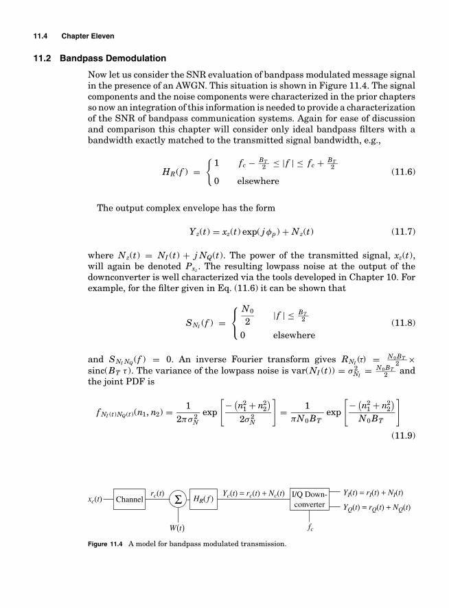
11.4 Chapter Eleven
11.2 Bandpass Demodulation
Now let us consider the SNR evaluation of bandpass modulated message signalin the presence of an AWGN. This situation is shown in Figure 11.4. The signalcomponents and the noise components were characterized in the prior chaptersso now an integration of this information is needed to provide a characterizationof the SNR of bandpass communication systems. Again for ease of discussionand comparison this chapter will consider only ideal bandpass filters with abandwidth exactly matched to the transmitted signal bandwidth, e.g.,
HR(f ) ={
1 fc − BT2 ≤ | f | ≤ fc + BT
2
0 elsewhere(11.6)
The output complex envelope has the form
Yz(t) = xz(t) exp( j φp) + Nz(t) (11.7)
where Nz(t) = NI (t) + j NQ(t). The power of the transmitted signal, xz(t),will again be denoted Pxz . The resulting lowpass noise at the output of thedownconverter is well characterized via the tools developed in Chapter 10. Forexample, for the filter given in Eq. (11.6) it can be shown that
SNI (f ) =⎧⎨⎩
N0
2| f | ≤ BT
2
0 elsewhere(11.8)
and SNI NQ (f ) = 0. An inverse Fourier transform gives RNI (τ) = N0 BT2 ×
sinc(BT τ ). The variance of the lowpass noise is var(NI (t)) = σ 2NI
= N0 BT2 and
the joint PDF is
f NI (t)NQ(t)(n1, n2) = 12πσ 2
Nexp
[− (n2
1 + n22
)2σ 2
N
]= 1
πN0 BTexp
[− (n2
1 + n22
)N0 BT
]
(11.9)
W t( )
Channelrc(t)
fc
Yc(t) = rc(t) + Nc(t)
YQ(t) = rQ(t) + NQ(t)
YI(t) = rI(t) + NI(t)xc(t) HR( f ) I/Q Down-
converterΣ
Figure 11.4 A model for bandpass modulated transmission.

Fidelity in Analog Demodulation 11.5
f NI(
t)N
Q(t
)(n 1
, n2)
0.2
0.15
0.1
0.05
04
4
3
3
2
2
1
1
0
0
n2
n1
−1
−1
−2
−2−3
−3−4−4
Figure 11.5 Plots of the joint PDF of NI (t) and NQ(t) for N0 BT = 2.
A plot of the density function for N0 BT = 2 is shown in Figure 11.5. The inputSNR to the demodulator is defined as
SNRi = Pxz
PNz
= Pxz
N0 BT= SNRb
WBT
= SNRbνB (11.10)
Consequently, the input SNR to the demodulator is both a function of thebaseband SNR and the spectral efficiency of the transmission. This is importantto note that broadcast FM typically has a lower input SNR than does broadcastAM since FM’s spectral efficiency is worse than AM’s spectral efficiency.
11.2.1 Coherent Demodulation
Many of the analog modulations considered in this text are demodulatedwith coherent demodulation structures and it is worth examining the noisecharacteristics of coherent demodulation structures. The coherent demodu-lator has a block diagram as given in Figure 11.6. The derotated noise,Nz(t) = Nz(t) exp(− j φp) in the coherent demodulator has the same statisticalcharacteristics as Nz(t). This is easy to show mathematically by
RNz(τ ) = E[Nz(t)N ∗
z (t − τ )] = E[Nz(t) exp(− j φp)N ∗z (t − τ ) exp( j φp)]
= E[Nz(t)N ∗z (t − τ )] = RNz(τ ) (11.11)

11.6 Chapter Eleven
m t( )Yz(t) = xz(t) exp( jfp) + Nz(t)Vz(t) = xz(t) + Nz(t)
exp(−jfp)
~MessageRecovery
Figure 11.6 The coherent demodulation structure.
Equation (11.11) shows that rotating the noise does not change the statisticalcharacteristics of the noise. Intuitively this makes sense because in examiningthe PDF plotted in Figure 11.5, the joint PDF of the lowpass noise is clearlycircularly symmetric. Any rotation of this PDF would not change the form of thePDF. This is mathematically proven in Problem 10.4. This circularly symmetricnoise characteristic and the results of Chapter 10 will allow us to rigorouslycharacterize the performance of coherent demodulation schemes.
11.3 Coherent Amplitude Demodulation
11.3.1 Coherent Demodulation
Given the tools developed so far the fidelity analysis of coherent AM demodu-lation systems is straightforward. Using the results of Section 11.2.1 we knowthat the baseband derotated noise is going to be zero mean, stationary, andGaussian with a PSD given as
SN I(f ) =
⎧⎨⎩
N0
2| f | ≤ BT
2
0 elsewhere(11.12)
Coherent DSB-AM
DSB-AM uses coherent demodulation. Recall the complex envelope form ofDSB-AM is xz(t) = Acm(t) so consequently the representative block diagramfor a DSB-AM demodulator in the presence of noise is given in Figure 11.7. Theoutput of the real operator has the form V I (t) = Acm(t) + N I (t) and the outputspectrum of the signal and the noise is shown in Figure 11.8(a). This signal
Yz(t) = Acm(t) exp( jfp) + Nz(t)Vz(t) = xz(t) + Nz(t)
exp(−jfp)
m t( )~
Re[•] HL( f )
Figure 11.7 The coherent demodulation structure for DSB-AM.

Fidelity in Analog Demodulation 11.7
W(a) Signal and noise spectrum (b) Noise model
~SNI( f )
Ac2|M( f )|2
f
N02
BR
NI(t) NL(t)HL( f )~
Figure 11.8 The DSB-AM demodulator noise processing.
and noise model is exactly the same form as seen in Section 11.1, consequentlythe filter, HL(f ), is subject to the same trade-offs between minimizing the noisepower and minimizing the signal distortion.
The filter, HL(f ), maximizes the SNR without signal distortion by being alowpass filter of bandwidth W. For simplicity in discussion the lowpass fil-ter will be assumed to be an ideal lowpass filter and to have the transferfunction
HL(f ) ={
1 | f | ≤ W
0 elsewhere(11.13)
The resulting message estimate for DSB-AM has the form m(t) = Acm(t) +NL(t). The distorting noise, NL(t), is produced by a lowpass filtering of N I (t)as shown in Figure 11.7(b). This output noise has a PSD given as
SNL(f ) = SN I(f ) |HL(f )|2 = SNI (f ) |HL(f )|2 =
⎧⎨⎩
N0
2| f | ≤ W
0 elsewhere(11.14)
The output noise power is var(NL(t)) = N0W and the output SNR is
SNRo = A2c Pm
N0W= Pxz
N0W= SNRb (11.15)
Recall the ET is the transmission efficiency defined as SNRo = ET SNRb, sothat it is clear here that ET = 1 so that coherent demodulation of DSB-AM hasthe same performance as an unmodulated signal. Since DSB-AM has ET = 1,two interesting insights are
1. The output SNR is exactly the same as the case where the signal was trans-mitted unmodulated. This implies that a coherent bandpass modulation anddemodulation process can result in no loss of performance compared to base-band transmission while greatly expanding the spectrum that can be usedfor transmission.

11.8 Chapter Eleven
2. Again the two things that affect the output SNR are the transmitted power1
and the message signal bandwidth. Consequently, transmitting video willcost more in terms of resources (transmitted power) than transmitting voicefor the same level of output performance.
Coherent SSB-AM
SSB-AM also uses coherent demodulation. Recall the complex envelope form ofSSB-AM is xz(t) = Ac(m(t)+ j m(t)∗hQ(t)), so, consequently, the representativeblock diagram of SSB-AM in noise is very similar to that in Figure 11.7. Theoutput of the real operator has the form V I (t) = Acm(t) + N I (t). This form isexactly the same form as DSB-AM. The resulting message estimate for DSB-AM has the form m(t) = Acm(t) + NL(t) where for the bandpass filter given inEq. (11.6)
SNL(f ) = SN I(f ) |HL(f )|2 =
⎧⎨⎩
N0
2| f | ≤ W
0 elsewhere(11.16)
The output noise power is var(NL(t)) = N0W and the output signal to noiseratio is
SNRo = A2c Pm
N0W(11.17)
Recall that the transmitted power of SSB-AM is Pxz = 2A2c Pm so this implies
that
SNRo = Pxz
2N0W= SNRb
2(11.18)
With this method of signal processing for demodulation of SSB-AM it is clearthat ET = 0.5 and it appears, at first glance, that SSB-AM is less efficient inusing the transmitted signal power than is an unmodulated system.
This loss in efficiency and fidelity of the message reconstruction can be reco-vered by better signal processing in the receiver. The methodology to improvethis efficiency is apparent when examining the signal and noise spectrum ofan upper sideband transmission shown in Figure 11.9. The bandpass filter inEq. (11.6) is passing all signal and noise within BT/2 Hz of the carrier frequency.This bandwidth is required in DSB-AM but clearly the receiver filter can bereduced in bandwidth and have a form
HR(f ) ={
1 fc ≤ | f | ≤ fc + BT2
0 elsewhere(11.19)
1Also the channel attenuation but we have chosen to normalize this to unity to simplify thediscussion

Fidelity in Analog Demodulation 11.9
Gxc( f )
SW( f )
fcf
fc + W
Figure 11.9 The signal and noise spectrum in SSB-AM reception.
The bandpass noise PSD then becomes
SNc (f ) =
⎧⎪⎨⎪⎩
N0
2fc ≤ | f | ≤ fc + BT
2
0 elsewhere(11.20)
Using the results of Chapter 10 gives
SNI (f ) = SNz(f ) + SNz(− f )4
=
⎧⎪⎨⎪⎩
N0
4| f | ≤ BT
2
0 elsewhere(11.21)
The effect of the choosing a filter that only passes the frequencies where themodulated signal is present instead of a filter like that in Eq. (11.6) is a reduc-tion by a factor of two in the output noise spectral density. By choosing the LPFto have bandwidth W the output SNR is then given as
SNRo = 2A2c Pm
N0W= 2Pxz ET
N0W= Pxz
N0W= SNRb (11.22)
The output SNR is exactly the same as the case where the signal was trans-mitted unmodulated so that ET = 1. This implies SSB-AM can also result inno loss of performance compared to a baseband or unmodulated transmissionusing only the W Hz of bandwidth.
11.4 Noncoherent Amplitude Demodulation
LC-AM uses noncoherent demodulation. Recall the complex envelope form ofLC-AM is xz(t) = Ac(1 + am(t)) with a chosen to allow distortion-free envelopedetection. Consequently, the representative block diagram of LC-AM demodu-lation in noise is given in Figure 11.10. Noting
Yz(t) = exp( j φp)( Ac[1 + am(t)] + Nz(t) exp(− j φp))
= exp( j φp)( Ac[1 + am(t)] + Nz(t))
= exp( j φp)( As(t) + Nz(t)) (11.23)

11.10 Chapter Eleven
Yz(t) = Ac[1 + am(t)] exp[jfp] + Nz(t)YD(t)
m t( )DCBlock
YA(t)|•| HL( f )
Figure 11.10 The noncoherent demodulation structure for LC-AM.
where As(t) is the amplitude modulated signal. This representation is inter-esting because the noise Nz(t) can be viewed as having the real componentin-phase with the received signal and the imaginary component in quadraturewith the received signal. A vector diagram of the output complex envelope fromthe downconverter at one point in time, t = ts, is given in Figure 11.11. SinceAs(t) = Ac[1+am(t)] is a real valued function, the phase of the received signal,rz(t), is entirely due to φp. The value of Y A(ts) is represented in Figure 11.11by the length of the vector Yz(ts). Considering this model, the output of theenvelope detector has the form
Y A(t) = |Yz(t)| =√
( Ac[1 + am(t)] + N I (t))2 + N 2Q(t)
=√
(As(t) + N I (t))2 + N 2Q(t) (11.24)
Using the results of Section 3.3.4, a transformation of random variables couldbe accomplished and the output could be completely characterized as a Ricean
NI(ts)
NQ(ts)
Yz(ts)YQ(t)
YI(t)
As(ts)
fp
~NQ(ts)
~NI(ts)
rz(ts)
Nz(ts)
Figure 11.11 A vector diagram representing one time sample of Yz(t).

Fidelity in Analog Demodulation 11.11
random variable [DR87]. While rigorous the procedure lacks intuition into theeffects of noise on noncoherent AM demodulation and will not be pursued inthis text.
To gain some insight into the operation of a LC-AM system a large SNRapproximation is invoked. At high SNR, Ac � |N I (t)| and Ac � |N Q(t)| whichimplies (see Problem 2.13) that
Y A(t) ≈√
(Ac[1 + am(t)] + N I (t))2 = Ac(1 + am(t)) + N I (t) (11.25)
Consequently, at high SNR only the noise in-phase with the carrier will make adifference in the output envelope and the output looks much like that given infor DSB-AM with the exception that the signal format is different. The outputof the DC block will be yD(t) = Acam(t) + N I (t) = me(t) + N I (t) and with alowpass filter bandwidth of W and using the same tools as above the outputSNR is
SNRo = Pme
PN I
= A2c a2 Pm
N0W(11.26)
Recall the definition of the message to carrier power ratio (MCPR) introducedin Chapter 6 so that
SNRo = A2c MCPRN0W
(11.27)
Since
Pxz = A2c (1 + MCPR) = A2
c
(1 + a2 Pm
)(11.28)
this implies that
SNRo = SNRbMCPR
1 + MCPR= Pme
Pxz
SNRb (11.29)
This implies that ET = MCPR1+MCPR = Pme
Pxzor, in words, the transmission effi-
ciency of LC-AM is the ratio of the power delivered at the demodulator outputto the transmitted power. The important thing to remember is that MCPR � 1for LC-AM to enable envelope detection so that the transmission efficiencyof LC-AM is also small. Consequently, at high SNR the only loss in perfor-mance in using a noncoherent demodulator for LC-AM is due to the wastedpower allocated to the carrier signal. The average MCPR of commercialLC-AM is usually less than 10% so the loss in SNR that occurs in usingLC-AM with envelope detection versus DSB-AM with coherent detection isgreater than 10 dB! This 10 dB lower fidelity is only compensated by the muchlower complexity of the envelope detector. This trade-off of fidelity versus com-plexity was deemed acceptable in the days before transistors. Today no compe-tent communication engineer would give up 10 dB for so little gain in ease ofimplementation.

11.12 Chapter Eleven
As SNRi gets smaller a threshold effect will be experienced in envelope detec-tion. The threshold effect occurs at SNRs below 10 dB so the analysis presentin this text is valid above a 10 dB input SNR and the details of the thresholdeffect should be considered carefully when operating at lower SNR. This impactof large noise and the resulting performance characteristics are not consideredin this introductory text but many excellent references cover this topic. Oneexample is [SBS66].
11.5 Angle Demodulations
The analysis of the performance of angle modulation demodulation algorithmsis quite complicated and a rich literature exists (e.g., [SBS66, Ric48]). The tackthat will be taken in this section is to simplify the analysis to provide the studenta good overview of the effects of noise on demodulation.
11.5.1 Phase Modulation
Phase modulation (PM) uses a noncoherent direct phase demodulator. Recallthe complex envelope of the received PM signal is
rz(t) = Ac exp[ j (kpm(t) + φp)] = Ac exp( j ϕs(t)) (11.30)
where ϕs(t) represents the overall received phase of the signal. Consequently,the representative block diagram of PM demodulation in noise is given inFigure 11.12. The output complex envelope from the downconverter at one pointin time, t = ts, is represented as in Figure 11.13 for an angle modulated signal.The output of the phase detector has the form
Y P (t) = tan−1(Y Q(t), Y I (t)) = kpm(t) + φp + ϕe(t) = ϕs(t) + ϕe(t) (11.31)
where ϕe(t) is the phase noise produced by the corrupting noise. Defining Nz(t)=Nz(t) exp (− j ϕs(t)) in a similar way as was done for coherent demodulation itcan be shown that
ϕe(t) = tan−1(NQ(t), Ac + NI (t)). (11.32)
Again using the results of Section 3.3.4, a transformation of random variablescould be accomplished and the output could be completely characterized [DR87].While rigorous the procedure lacks intuition into the effects of noise on nonco-herent PM demodulation.
Yz(t) = Ac[ j(kpm(t) + fp] + Nz(t)YD(t)
m t( )PhaseUnwrap
YP(t) DCBlock
arg (•) HL( f )
Figure 11.12 The noncoherent demodulation structure for PM.

Fidelity in Analog Demodulation 11.13
NI(ts)
NQ(ts)
Yz(ts)YQ(t)
YI(t)
Ac
Yp(ts)
js(ts)
je(ts)
~NQ(ts)
~NI(ts)
rz(ts)
Nz (ts)
Figure 11.13 A vector diagram representing one time sample of Yz(t) for anglemodulation.
Again to gain some insight into the operation of a PM system a large SNRapproximation is invoked. At high SNR Ac � |NI (t)| and Ac � |NQ(t)|, whichimplies (see Problem 2.13) that
ϕe(t) ≈ tan−1
(NQ(t)
Ac
)≈ NQ(t)
Ac(11.33)
It is important to note that the inverse tangent in Eq. (11.33) is the morecommon one argument inverse tangent function. The important insight gainedfrom this high SNR approximation is that the phase noise produced is a functionof the noise in quadrature to the modulated signal. At high SNR the outputphase noise is approximately Gaussian, zero mean (i.e., E[NQ(t)] = 0) and theoutput noise variance is a function of both the input noise and the input signal(i.e., E[ϕ2
e (t)] = E[N 2Q(t)]/A2
c ). The following approximation is also valid at highSNR [SBS66]
RNQ(t, τ ) = RNQ (τ ) = RNI (τ ) (11.34)
Consequently, the output phase noise is Gaussian, zero mean and has an ap-proximate PSD of Sϕe (f ) = SNI (f )/A2
c . The signal and noise spectrum are asshown in Figure 11.14(a).

11.14 Chapter Eleven
W
(a) Signal and noise spectrum. (b) Noise model.
SNI( f )
Sje( f ) =
kp2|M( f )|2
f
N02Ac
2
BT2
Ac2
je(t) NL(t)HL( f )
Figure 11.14 The PM demodulator noise processing.
The effect of the noise due to the remainder of the processing needed to recoverthe message can also be characterized. The DC block removes the term due toφp and this section will assume the DC block is very small notch in frequencyand does not impact the noise power significantly. Since BT > 2W for PMthe noise power can be reduced by filtering the output of the DC block. Themodel for the noise processing in PM is modeled with Figure 11.14(b). Assumingthe lowpass filter is ideal and has a bandwidth of W then output messageestimate has the form m(t) = kpm(t) + NL(t) where for the bandpass filtergiven in Eq. (11.6)
SNL(f ) = Sϕe (f ) |HL(f )|2 = SNI (f )A2
c|HL(f )|2 =
⎧⎨⎩
N0
2A2c
| f | ≤ W
0 elsewhere(11.35)
The output noise power is var(NL(t)) = N0W/A2c and the output signal to noise
ratio is (recall Pxz = A2c for PM)
SNRo = A2c k2
p Pm
N0W= k2
p PmPxz
N0W= k2
p PmSNRb (11.36)
The transmission efficiency is ET = k2p Pm. The resulting SNR performance for
PM has four interesting insights
1. Again two parameters that affect SNRo are the transmitted power and themessage signal bandwidth (much like AM systems). In addition, there is athird parameter ET = k2
p Pm that can be chosen by the designer.
2. At high SNR the effective performance can be improved an arbitrary amountby increasing kp. If k2
p Pm > 1, then using a nonlinear modulation like PMallows the designer to actually get a performance better than that achievedat baseband.
3. Recall kp also increases the output bandwidth of a PM signal. Hence PMallows an engineer to trade spectral efficiency for SNR performance. Such atrade-off is not possible with AM.

Fidelity in Analog Demodulation 11.15
+ Nz(t)Yz(t) = Ac expYD(t)
m t( )PhaseUnwrap
YP(t) ddt
arg(•)
HL( f )j k f m λ( )dλ + φp−∞
t
∫⎛
⎝⎜⎞
⎠⎟⎡
⎣⎢⎢
⎤
⎦⎥⎥
Figure 11.15 The noncoherent demodulation structure for FM.
4. For large values of kp phase unwrapping becomes increasingly difficult. Con-sequently, there is a practical limit to the size of kp and hence a limit to thegain in SNR one can achieve compared to an unmodulated system.
As SNRi gets smaller a threshold effect will be experienced in PM demod-ulation and that will not be discussed in this introductory text. An interestedreader should, for example, see [SBS66].
11.5.2 Frequency Modulation
FM has a noncoherent demodulation structure much like that of PM. Recallthe complex envelope of the received FM signal is
rz(t) = Ac exp[
j(
kf
∫ t
−∞m(λ)dλ + φp
)]= Ac exp( j ϕs(t)) (11.37)
where ϕs(t) represents the overall received phase of the signal. The demodula-tion structure for FM is shown in Figure 11.15. The output of the phase detectorhas the form
Y P (t) = tan−1(Y Q(t), Y I (t)) = kf
∫ t
−∞m(λ)dλ + φp + ϕe(t) = ϕs(t) + ϕe(t)
(11.38)Again defining Nz(t) = Nz(t) exp (− j ϕs(t)) it can be shown that
ϕe(t) = tan−1(NQ(t), Ac + NI (t)) (11.39)
Again a complete statistical characterization is possible but lacks the intuitionthat we want to achieve in this course.
The effect of the noise due to the remainder of the processing needed torecover the message can also be characterized using similar approximations aswas done for PM. We can use the same high SNR approximations as with PMto gain insight into the performance of FM. Recall at high SNR
ϕe(t) ≈ tan−1
(NQ(t)
Ac
)≈ NQ(t)
Ac(11.40)
so that the noise at the output of the direct phase detector is well modeled asGaussian, zero mean and has a PSD of Sϕe (f ) = SNI (f )/A2
c . Since the deriva-tive operation is a linear system the processing after the phase conversionnonlinearity can be represented as the cascade of two linear systems as shownin Figure 11.16(a). The derivative operation removes the phase offset, φp so

11.16 Chapter Eleven
je(t)Nf (t)Hd ( f )
NL(t)HL( f )
(a) Processing block diagram
0
1
2
3
4
5
f(b) Noise spectrum
SNL( f )
SNf( f )
BT
2
BT
2− −W −W
Figure 11.16 Noise processing in an FM demodulator.
that YD(t) = kf m(t) + dϕe(t)/dt = kf m(t) + Nf (t). The derivative is a linearsystem with a transfer function of
Hd (f ) = j 2π f (11.41)
so at high SNR the output power spectrum of Nf (t) is approximated as
SNf (f ) = SNI (f )A2
c|Hd (f )|2 =
⎧⎪⎨⎪⎩
2N0π2 f 2
A2c
| f | ≤ BT2
0 elsewhere(11.42)
This output spectrum is plotted in Figure 11.16(b). Interestingly the derivativeoperation has colored the noise (PSD is not flat with frequency) as the derivativeoperation tends to accentuate high frequencies and attenuate low frequencies.The next section will demonstrate how engineers used this colored noise totheir advantage in high fidelity FM based communications. The final outputafter the lowpass filter can also be characterized using the tools developed inthis course. The final output after an ideal filter with a bandwidth of W has theform m(t) = kf m(t) + NL(t) where
SNL(f ) =
⎧⎪⎨⎪⎩
2N0π2 f 2
A2c
| f | ≤ W
0 elsewhere(11.43)
The resulting signal power is Ps = k2f Pm and the noise power is given as
PN =∫ ∞
−∞SNL(f )df = 2N0π
2
A2c
∫ W
−Wf 2df = 4N0π
2W 3
3A2c
(11.44)

Fidelity in Analog Demodulation 11.17
so that the resulting output SNR is
SNRo = 3A2c k2
f Pm
4N0π2W 3 = 3k2f Pm
4π2W 2
Pxz
N0W= 3k2
f Pm
4π2W 2 SNRb (11.45)
Here it is clear that ET = 3k2f Pm
4π2W 2 . Since kf is a parameter chosen by the designerthe transmission efficiency of FM is again selectable. Recalling that kf = 2π f k ,where f k is the frequency deviation constant (measured in Hz/V), gives a moresuccinct form for the output SNR as
SNRo = 3k2f Pm
4π2W 2 SNRb = 3 f 2k Pm
W 2 SNRb (11.46)
The resulting SNR performance for FM has two interesting insights
1. At high SNR the effective performance can improve an arbitrary amountby increasing f k . Recall f k also increases the output bandwidth of a FMsignal. Hence FM also allows an engineer to trade spectral efficiency forSNR performance. Edwin Armstrong was the first person to realize that thistrade-off was possible.
2. The output noise from an FM demodulator is not white (flat with frequency).The sequel will demonstrate how this colored noise characteristic can beexploited.
As SNRi gets smaller a threshold effect will be experienced in FM demod-ulation but that will not be discussed in this introductory text. An interestedreader should, for example, see [SBS66].
11.6 Improving Fidelity with Pre-Emphasis
The insights gained in analyzing the noise in the previous section have helpedengineers understand techniques to improve the output SNR in angle demodu-lations. The three insights that led to this improved technique are
1. The noise at the output of the differentiator is not white so that noise poweris larger at higher frequencies.
2. The power of the noise tends to be distributed differently over frequency thanthe power of the signal. A fairly typical example of this different distributionis shown in Figure 11.17.
3. The received signal power, Pxz = Prz , is not a function of the message signal.
Consequently, if one can process the signal at the transmitter and receiverin such a way that the signal is unchanged and that the high frequency com-ponents of the noise are de-emphasized then a significant SNR advantage canbe gained. The way to achieve this gain is shown in Figure 11.18 and hasbeen denoted pre-emphasis and de-emphasis in the communications literature.

11.18 Chapter Eleven
0
1
2
3
4
5
f−W W
Pow
er S
pect
rum Noise Signal
Figure 11.17 Examples of the signal and noise spectrum at the output of an FMdemodulator.
The idea is to pre-emphasize the high frequencies of the signal before FMmodulation with a linear filter, HE (f ). This pre-emphasis will not change thetransmitted signal power which will still be Pxz = A2
c . This pre-emphasis willimpact the transmitted spectrum some as this adding gain to the high frequencycomponents of the message spectrum could increase the peak frequency devia-tion. At the receiver the de-emphasis filter, HD(f ), is chosen to give an overallunity gain to the message signal, e.g.,
|HE (f )HD(f )| = 1 | f | ≤ W (11.47)
Denoting the input and output of the de-emphasis filter as
mE (t) = mE (t) + NL(t) m(t) = m(t) + ND(t) (11.48)
it is clear this de-emphasis filter will further decrease the output noise powersince the PSD of ND(t) will be given as
SND (f ) = SNL(f ) |HD(f )|2 (11.49)
The actual amount of SNR gain will be a function of the specific filter transferfunctions and the spectral characteristics of the message signal. In practicalsystems this gain is typically over 10 dB. Some specific examples will be exploredin the homework.
It is interesting to note that commercial analog “FM” broadcast in the UnitedStates uses pre-emphasis and de-emphasis. Since a pre-emphasis circuit effec-tively is behaving like a differentiator, the true transmitted signal in broadcast
yc(t)xc(t) ChannelAngle
DemodulatorAngle
ModulatormE(t)m(t) HD( f )HE( f )
m(t)mE(t)
Figure 11.18 Block diagram of pre-emphasis and de-emphasis in FM systems.

Fidelity in Analog Demodulation 11.19
radio is actually a hybrid of phase modulation and frequency modulation. It isinteresting that this modulation is known in popular culture as FM while, infact, it is not a true frequency modulation of the message signal.
11.7 Final Comparisons
A summary of the important characteristics of analog modulations is given inTable 11.1. At the beginning of Chapter 5 the performance metrics for ana-log communication systems were given as: complexity, fidelity, and spectralefficiency.
In complexity the angle modulations offer the best characteristics. Trans-mitters for all of the analog modulations are reasonable simple to implement.The most complicated transmitters are needed for VSB-AM and SSB-AM. Thecomplexity is needed to achieve the bandwidth efficiency. The angle modula-tions have a transmitted signal with a constant envelope. This characteristicmakes designing the output power amplifiers much simpler since the linear-ity of the amplifier is not a significant issue. Receivers for LC-AM and anglemodulation can be implemented in simple noncoherent structures. Receiversfor DSB-AM and VSB-AM require the use of a more complex coherent struc-ture. SSB-AM additionally will require a transmitted reference for automaticcoherent demodulation and operation.
In spectral efficiency SSB-AM offers the best characteristics. SSB-AM isthe only system that achieves 100% efficiency. DSB-AM and LC-AM are 50%efficient. VSB-AM offers performance somewhere between SSB-AM andDSB-AM. Angle modulations are the least bandwidth efficient. At best theyachieve EB = 50%, and often much less.
In terms of fidelity there is a variety of options. Coherent demodulation offersperformance at the level that could be achieved with baseband transmission.Noncoherent demodulation schemes can have a threshold effect at low SNR butabove threshold provide very good performance. The only difference betweencoherent demodulation and noncoherent demodulation of LC-AM at high SNRis the transmission inefficiency needed to make envelope detection possible.
TABLE 11.1 A comparison of the trade-offs in analog modulation
Spectral TX RX FidelityModulation Efficiency Complexity Complexity
DSB-AM 50% moderate moderate ET = 1
LC-AM 50% moderate small ET ≈ MCPRExperiences a threshold effect
VSB-AM > 50% large large 0.5 ≤ ET ≤ 1
SSB-AM 100% large large 0.5 ≤ ET = 1
PM < 50% small moderate Can trade-off BW for ET by choice of kpExperiences a threshold effect
FM < 50% small moderate Can trade-off BW for ET by choice of kfExperiences a threshold effectColored noise in demodulationcan be exploited

11.20 Chapter Eleven
Angle modulation when operated, above threshold offers a trade-off betweenoutput SNR at the demodulator and the transmitted signal bandwidth. In gen-eral, angle modulations offer the ability to trade bandwidth efficiency for outputSNR. This ability is not available in AM modulation and is the reason FM isused for high fidelity broadcast in the United States. Finally, the noise spec-trum at the output of an FM demodulator is nonwhite. This nonwhite spectralcharacteristic can be taken advantage of by appropriate signal processing to im-prove the output SNR even further. This idea of pre-emphasis and de-emphasisis an excellent example of communication engineers getting significant perfor-mance advantages for little cost in complexity by simply understanding a littlecommunication theory.
11.8 Homework Problems
Problem 11.1. For DSB-AM with a coherent demodulation, if the receiver phasereference has an error of φe compute the output SNR. How big can φe be and yetlimit the degradation in SNR to less than 3 dB from the optimum performance?
Problem 11.2. Consider a bandpass Gaussian noise at the input to a demodulatorwith a spectrum given as
SNc (f ) = 0.01 fc − 200 ≤ | f | ≤ fc + 300
= 0 elsewhere (11.50)
in the system given in Figure 11.4. Assume that the modulation is DSB-AM with
rc(t) = Acm(t)√
2 cos(2π fct + φp) (11.51)
where Ac = 1 and the message signal has a W = 60 Hz bandwidth and powerPm = 10 W. Using the signals Y I (t) and Y Q(t) as inputs and assuming youknow φp
(a) Define Nz(t) = Nz(t) exp(− j φp). Give the joint PDF of N I (t0) and N Q(t0),f N I (t0)N Q(t0)(n1, n2) in a 1-� system for a fixed t0.
(b) Find the best demodulator structure that leaves the signal undistorted andmaximizes the SNR.
(c) Give the maximum SNR.
Problem 11.3. The following complex envelope is received
Yz(t) = (cos(200πt) + sin(20πt)) exp[ j π/7] + Nz(t) (11.52)
The bandpass noise is characterized with
SNz(f ) ={
0.005 | f | ≤ 4000
0 elsewhere(11.53)

Fidelity in Analog Demodulation 11.21
(a) What kind of modulation is being used and what is the message signal (upto a constant).
(b) Sketch the block diagram of the demodulation processing assuming thatthe demodulator knows φp = π/7.
(c) If the lowpass filtering in the message recovery portion of the demodula-tor is ideal and unit gain with 4000 Hz bandwidth compute the outputSNR.
(d) What ideal lowpass filter bandwidth would optimize the output SNR?
(e) Could an ideal bandpass filter at the output of the demodulator improveperformance? If so give the optimum filter specifications and the resultingSNR.
Problem 11.4. In discussing noise in angle modulation we had defined a derotatednoise
Nz(t) = Nz(t) exp (− j ϕs(t)) (11.54)
This problem will examine the approximations made in the text and see howthey can be justified. Assume the bandpass filter at the receiver front end isideal and has a bandwidth of BT = 2( f p + W ) and is symmetric around fc sothat RNI NQ (τ ) = 0.
(a) Find RNI (τ ).
(b) Show that NQ(t) = NQ(t) cos(ϕs(t)) − NI (t) sin(ϕs(t)).
(c) Compute RNQ(t1, τ ) = E[NQ(t1)NQ(t1 − τ )].
(d) Since the result in (c) is a function of ϕs(t1) − ϕs(t1 + τ ) show that ϕs(t1) −ϕs(t1 + τ ) ≈ 2π fd (t1)τ .
(e) Show that only when the instantaneous frequency deviation is large, willRNQ
(t1, τ ) be much different than RNQ (τ ).
(f) Plot RNQ(t1, τ ) and RNQ (τ ) for fd (t1) = f p and fd (t1) = f p/2.
Problem 11.5. A student from another university claims that the optimal receiverfor SSB-AM is given in Figure 11.19. The student argues that the quadrature
Yz(t) = xz(t)exp( jfp) + NZ(t)me(t) + NT(t)
exp( jfp)
Re [•]
Im [•]
ΣΣ
H2( f )
HL( f )Vz(t) = xz(t) + Nz(t)
~
Figure 11.19 An alternative demodulator for SSB-AM.

11.22 Chapter Eleven
component contains information related to the message signal and you shoulduse this information in the optimum demodulator. You begin to doubt the edu-cation you received and set about to verify whether Prof. Fitz is right in whathe presented in this chapter or if the other student got a better education atthe other university. For this problem assume the filter at the front end of theradio is given as Eq. (11.19) and that the noise output from H2(f ) is denotedNQ(t).
(a) Show that for the case of upper sideband transmission via SSB-AM if H1(f )is a lowpass filter of bandwidth W and that
H2(f ) ={
j sgn(f ) | f | ≤ W
0 elsewhere(11.55)
then me(t) = 2Acm(t). (It doesn’t look good for Prof. Fitz as the signal in thealternative demodulator is twice as big what Prof. Fitz presented!)
(b) Denote NI (t) as the output of H1(f ) and NQ(t) as the output of H2(f ) andshow that
var(NT (t)) = var(NI (t)) + var(NQ(t)) + 2RNI NQ(0) (11.56)
(c) Compute E[N 2I (t)].
(d) Compute E[N 2Q(t)].
(e) What is SNI NQ(f )? (Feel free to use the results in Problem 10.10.)
(f) What is RN I NQ(0)?
(g) What is the output SNR? Which structure would you choose for implement-ing a SSB-AM demodulator Figure 11.19 or Figure 11.7 and why?
Problem 11.6. This problem considers the demodulation of stereo broadcast con-sidered in Problem 7.24.
(a) Postulate a demodulation structure for stereo broadcast that has as outputsmS (t) and mD(t). Assume a coherent demodulation for the DSB-AM signalis possible2.
(b) Using the assumption that the power of the sum and difference signals areboth Pm calculate the output SNR for the estimation of mS (t).
(c) Using the assumption that the power of the sum and difference signals areboth Pm calculate the output SNR for the estimation of mD(t). The outputSNRs are different, why?
(d) Using these results postulate a mechanism to trigger the stereo indicatorlight based on the SNR differences seen on the two channels.
2This coherent demodulation is achieved by processing the pilot tone.

Fidelity in Analog Demodulation 11.23
Problem 11.7. Consider an FM system with W = 15 kHz, Pm = 1, max |m(t)| = 3,and an input noise characterized as
SW (f ) = 10−6 (11.57)
Assume the receiver filter is an ideal bandpass filter with a bandwidth equalto Carson’s bandwidth.
(a) Define the bandpass SNR for an angle modulated signal to be
SNRbp = A2c
E[N 2
c (t)] (11.58)
and find the value of Ac (as a function of f k) needed to provide SNRbp =10 dB (so that the demodulator will be operating above threshold and thesmall noise approximation is valid).
(b) With the Ac as specified in (a) choose an f k such that SNRo = 30 dB.
(c) Broadcast radio in the United States was originally designed with only oneaudio channel of 15 kHz such that D = 5, for the system parameters givenin this problem with Ac as specified in (a) what would the SNRo for thisoriginal broadcast standard?
Problem 11.8. Assume a communication system uses DSB-AM and the receivedsignal is corrupted by a white Gaussian noise with a one-sided noise spectraldensity of N0 = 10−6. Specify the optimum demodulator and find the receivedsignal power, Pxz , that would be needed to achieve a SNR = 10 dB for
(a) W = 4 kHz
(b) W = 15 kHz
(c) W = 4.5 MHz
Problem 11.9. A simple pre-emphasis filter which is commonly used in practiceis given by
Hpe(f ) = 1 + j ff0
(11.59)
where f0 = 2.1 kHz. The corresponding de-emphasis filter is a simple lowpassfilter having the form
Hd e(f ) = 11 + j f
f0
(11.60)
(a) Defining Ipde as the noise power improvement ratio when using pre-emphasis/de-emphasis, calculate Ipde for this filter combination. Sorry tosay this will require a little calculus!

11.24 Chapter Eleven
xz(t) Yz(t)mE(t) m t( )DSB-AMModulator
ChannelDSB-AM
Demodulatorm(t)
∫(Σ)dt
Figure 11.20 A pre-emphasis and de-emphasis system for DSB-AM.
(b) For the case of mono FM broadcast ( f p = 75 kHz, W = 15 kHz) and anbandpass SNR of
Pxz
BT N0(11.61)
calculate the output signal to noise ratio with and without pre-emphasis/de-emphasis.
(c) For the same parameters as in (b), calculate the value of
SNRb = Pxz
W N0(11.62)
Recall that this is the optimum output SNR for an AM system.
(d) What is the performance improvement of FM modulation (above threshold)with and without pre-emphasis/de-emphasis over DSB-AM modulation?
Problem 11.10. You have just started your job at Asprocket Systems and you anda senior Asprocket engineer have been given the job of improving the perfor-mance of a DSB-AM radio station that will be deployed by the Outer Boehtaviangovernment for news spinning (propaganda). The senior engineer said that oneway to improve noise performance is to use pre-emphasis and de-emphasis inthe radios and proposed the system shown in Figure 11.20. You have a bad feel-ing about this as in your high powered education you were never taught aboutpre-emphasis and de-emphasis being used in AM systems. Analyze the systemdesign by the senior Asprocket engineer and decide whether it is useful or not.Justisty your answers by computing the output SNR = A2
c Pm
PNand comparing that
to SNRb = PxzPN
. For simplicity of computation assume m(t) is a random processwith a power spectrum
SM(f ) =⎧⎨⎩
Pm
2W| f | ≤ W
0 elsewhere(11.63)
Problem 11.11. (JG) Consider the baseband communication system, shown inFigure 11.21, where the signal and noise are both modeled as zero mean,
M t( )M t( )
N t( )
Xz(t)Ac Σ
Figure 11.21 A baseband noise system.

Fidelity in Analog Demodulation 11.25
Yz(t)AcXz(t)
N(t)
M t( )M t( ) Σ H2( f )H1( f )
Figure 11.22 A baseband noise system with transmitter and receiverfiltering.
WSS, random processes with power spectral densities SM(f ) and SN (f ),respectively.
SM(f ) ={ 1
2W | f | < W
0 | f | > WSN (f ) =
⎧⎪⎪⎨⎪⎪⎩
aN0 | f | < W2
bN0W2 < | f | < W
0 | f | > W
(11.64)
(a) What is the SNR in the received signal M(t)?
(b) The system is modified by including transmit and receive filters as shownin Figure 11.22. Design H2(f ) to whiten the noise process for | f | < W .
(c) Given your choice of H2(f ), design H1(f ) to achieve distortionlesstransmission.
(d) What is the SNR improvement in the new system versus the old system?
Problem 11.12. Consider a situation where a message signal is modeled as astationary Gaussian random process with a PSD given in Figure 11.23. Assumethis signal is corrupted by an additive white Gaussian noise with a one–sidedspectral density of N0. This combined signal plus noise is put into an ideallowpass filter that has a bandwidth of W . Choose W to optimize the outputSNR and give the value of this optimum SNR.
Problem 11.13. Consider the situation presented in Example 11.1. Replace theLPF with another filter that would achieve an output with SNR = 12 dB.
−200 200
1
f
SM( f )
Figure 11.23 The power spectrum of the message signal.

11.26 Chapter Eleven
11.9 Example Solutions
(a) The modulation is DSB-AM. Recall that Yz(t) = xz(t) exp[ j φp] + Nz(t) andthe message signal is real. Since there is no time varying angle the signalis clearly not an angle modulated. There is no DC offset in the complexenvelope so it is not LC-AM. The received signal spectrum is two sided sono quadrature modulation was implemented. If DSB-AM has been imple-mented then the message signal is m(t) = A(cos(200πt) + sin(20πt)) whereA = 1/Ac.
(b) See Figure 11.7 with φp = π/7.
(c) Using the results of Chapter 9 it is known that
SNL(f ) = SNI (f )|HL(f )|2 (11.65)
The results of Chapter 10 we have
SNI (f ) = SNz(f ) + SNz(− f )4
(11.66)
and finally
SNL(f ) = SNI (f )|HL(f )|2 ={
.0052 , | f | ≤ 4000
0, elsewhere
Consequently, since the noise power is given as
PN = E[N 2
L(t)] = ∫ ∞
−∞SNL(f )df = 20. (11.67)
The output signal power is easily computed using Parseval’s theorem to bePs = 0.5 + 0.5. The resulting SNR = 0.05.
(d) Since the message bandwidth is 100 Hz, so the ideal lowpass filter has100 Hz bandwidth. The new output noise spectral density is
SNL = SNI |HL(f )|2 ={
.0052 , | f | ≤ 100
0, elsewhere
and the resulting noise power is
PN = E[N 2
L(t)] = ∫ ∞
−∞SNL(f )df = 0.5. (11.68)
The resulting SNR in this case is SNR = 2.

Fidelity in Analog Demodulation 11.27
(e) The message bandwidth is 100 Hz, but we don’t have any signal from 0 to10 Hz, if we use a bandpass filter from 10 to 100 Hz we can improve SNR.
SNL = SNI |HL(f )|2 ={
.0052 , 10 ≤ | f | ≤ 100
0, elsewhere
S N R = 0.5 + 0.50.35
= 2.22
Problem 11.5. This architecture was actually proposed in another textbook andsupposedly used in practice. The analysis of this problem is a classic exampleof how understanding the theory of random processes can ensure that you arenot fooled by incorrect hueristic arguements in engineering. The answer is“yes”, there is information in the quadrature channel of a SSB-AM demodulatedsignal about the message but in terms of possible achieved SNR it is redundantinformation.
(a) Denote the noiseless signal out of H1(f ) as m1(t) then m1(t) = Acm(t). Alsodenote the noiseless signal out of H2(f ) as m2(t) then the output Fouriertransform is given as
M2(f ) = Ac H2(f )Mh(f ) = Ac ( j sgn(f )) (− j sgn(f )) M(f ) = Ac M(f )(11.69)
Consequently, me(t) = m1(t) + m2(t) = 2Acm(t).
(b) Since NT (t) = NI (t) + NQ(t) it is straightforward to show that
E[N 2
T (t)] = E
[(NI (t) + NQ(t))2]
= E[N 2
I (t)]+ E[N 2
Q(t)]+ 2E[NI (t)NQ(t)]
= var(NI (t)) + var(NQ(t)) + 2RNI NQ(0) (11.70)
(c) From the text we have that
SNz(f ) =
{N0 0 ≤ f ≤ W
0 elsewhere(11.71)
and
SN I(f ) = SN Q
(f ) =⎧⎨⎩
N0
4−W ≤ f ≤ W
0 elsewhere(11.72)
Since from Chapter 9 it is known that
SNI(f ) = SN I
(f ) |H1(f )|2 (11.73)

11.28 Chapter Eleven
this implies that
var(NI (t)) =∫ ∞
−∞SNI
(f )df = N0W2
(11.74)
(d) Similarly,
SNQ(f ) = SN I
(f ) |H2(f )|2 (11.75)
so that
var(NQ(t)) =∫ ∞
−∞SNQ
(f )df = N0W2
(11.76)
(e) From Chapter 10 it is known that
SNI NQ(f ) = SNz(− f ) − SNz(f )
j 4=⎧⎨⎩
j N0sgn(f )4
−W ≤ f ≤ W
0 elsewhere(11.77)
Problem 10.10 gives the result
SNI NQ(f ) = SN I N Q
(f )H ∗2 (f )H1(f ) =
⎧⎨⎩
j N0sgn(f )4
− j sgn(f ) −W ≤ f ≤ W
0 elsewhere
(11.78)
=⎧⎨⎩
N0
4−W ≤ f ≤ W
0 elsewhere(11.79)
(f) Recall that
RNI NQ(0) =
∫ ∞
−∞SNI NQ
(f )df = N0W2
(11.80)
(g) The output SNR is
SNRo = Pme
var(NT (t))= 4A2
c Pm
2N0W= 2A2
c Pm
N0W(11.81)
This output SNR is exactly the same as for the demodulation architecturegiven in the text and yet it is more complicated than the architecture givenin class. Consequently, a good engineer would prefer the architecture givenin class.

Fidelity in Analog Demodulation 11.29
11.10 Miniprojects
Goal: To give exposure
■ to a small scope engineering design problem in communications.■ to the dynamics of working with a team.■ to the importance of engineering communication skills (in this case oral pre-
sentations).
Presentation: The forum will be similar to a design review at a company(only much shorter) The presentation will be of 5 minutes in length with anoverview of the given problem and solution. The presentation will be followedby questions from the audience (your classmates and the professor). All teammembers should be prepared to give the presentation.
11.10.1 Project 1
Project Goals: To examine the validity of the large SNR approximation thatwas made in the analysis of the demodulation fidelity of LC-AM.
Consider a received signal of the form
Yz(t) = As + Nz(t) (11.82)
where S N R = A2s
2σ 2NI
. As a minimum plot a sample histogram with at least
10,000 points of the resulting values of the random variable Y A(t) for S N R =10 dB and S N R = 0 dB. Make an assessment of the SNR where the approxi-mation given in Eq. (11.25) is valid.
11.10.2 Project 2
Project Goals: To examine the validity of the large SNR approximation thatwas made in the analysis of the demodulation fidelity of angle modulations.
Consider a received signal of the form
Yz(t) = As + Nz(t) (11.83)
where S N R = A2s
2σ 2NI
. As a minimum plot a sample histogram with at least 10,000
points of the resulting values of the random variable Y P (t) for S N R = 10 dBand S N R = 0 dB. Make an assessment of the SNR where the approximationgiven in Eq. (11.33) is valid.

This page intentionally left blank

Part
4Fundamentals of Digital
Communication
Copyright © 2007 by The McGraw-Hill Companies. Click here for terms of use.

This page intentionally left blank

Chapter
12Digital Communication Basics
The problem that is of interest in this text is point-to-point binary data com-munications. The system model for such a communication system is given inFigure 12.1. A source of binary encoded data with a total of Kb bits is presentand it is desired to transmit this data to a binary data sink across a physicalchannel. The data output by the source is represented by a Kb × 1 dimen-sional vector, �I , whose components take values 0,1. The 2Kb different wordswill be enumerated with an index i = 0, . . . , 2Kb − 1. It should be noted thatin general each of these Kb bit words is not equally likely to be sent. A proba-bility πi will be associated with the sending of each word. This informationvector to be sent is then mapped into one of 2Kb analog waveforms repre-sented by the waveform xi(t). Denote Tp as the largest support of all thexi(t), then the transmission rate or bit rate of the system is Wb = Kb/Tp bitsper second. The transmitted waveform is put through a channel of some sortand corrupted by noise or interference. The composite received signal, Yc(t), isthen used to estimate which one of the possible vectors led to the transmittedwaveform. This estimate is denoted �I and this estimate is passed to the datasink.
It should be noted that point-to-point data communications is but the simplestabstraction of the data communications reality. This point-to-point communi-cation is often referred to as physical layer communications. There are manyhigher layers of abstraction in data communication. These higher layers dealwith concepts like how do multiple users access a shared communication media,how is a communication path established in a multiple hop network, how do ap-plications communicate across the network. These issues are typically coveredin the curriculum in a course on communication networks. Typical textbooksthat explore the details of communication networks are [KR04, LGW00, Tan02].The student interested in the details of networked communication should takethese courses or read these textbooks.
12.1
Copyright © 2007 by The McGraw-Hill Companies. Click here for terms of use.

12.2 Chapter Twelve
Yc(t)Rc(t)Xc(t) ChannelBinary Data
SinkBinary Data
SourceSignal
DemodulatorData
Modulator
W(t)
Σ I^
I
Figure 12.1 A model for point-to-point data communication.
12.1 Digital Transmission
In exactly the same way as in analog communication, digital communication hasa modulator and demodulator. The modulator produces an analog signal thatdepends on the digital data to be communicated. This analog signal is trans-mitted over a channel (a cable or radio propagation). The demodulator takesthe received signal and constructs an estimate of the transmitted digital data.There are two types of digital communications that are implemented in practice:Baseband data communications as exemplified by compact disc recordings ormagnetic recording (e.g., computer hard drives) and carrier modulated datacommunications as exemplified by computer voiceband modems or radio mod-ems used in wireless local area computer networks. In this text we want tohave a unifying framework that enables the material that is learned to applyto either baseband or bandpass data communications. As with analog commu-nications, the complex envelope notation is used to achieve this goal. The onlycaveat that needs to be stated is that baseband data communication will al-ways have a zero imaginary component, while for bandpass communicationsthe imaginary component of the complex envelope might be nonzero.
12.1.1 Digital Modulation
Definition 12.1 Digital modulation is a transformation of �I into a complex envelope,Xz(t).
This transformation is equivalent to transforming m(t) into a bandpasssignal, Xc(t). In a slight deviation for digital communications, as compared toanalog communications, the transmitted waveform will be considered a randomprocess. The randomness in this transmitted waveform will be the randominformation bits, �I , that are being transmitted. The digital modulationprocess, Xz(t) = �m( �I ) is represented in Figure 12.2. It should be emphasized
xz(t) xc(t)Γm (•) I/QUp-converter
I
Figure 12.2 The digital modulation process. Note the IQupconverter is given in Figure 4.4.
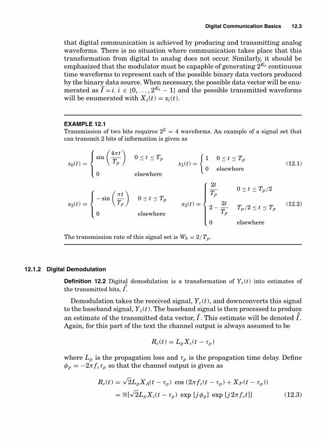
Digital Communication Basics 12.3
that digital communication is achieved by producing and transmitting analogwaveforms. There is no situation where communication takes place that thistransformation from digital to analog does not occur. Similarly, it should beemphasized that the modulator must be capapble of generating 2Kb continuoustime waveforms to represent each of the possible binary data vectors producedby the binary data source. When necessary, the possible data vector will be enu-merated as �I = i. i ∈ {0, . . . , 2Kb − 1} and the possible transmitted waveformswill be enumerated with Xz(t) = xi(t).
EXAMPLE 12.1Transmission of two bits requires 22 = 4 waveforms. An example of a signal set thatcan transmit 2 bits of information is given as
x0(t) =
⎧⎪⎨⎪⎩
sin
(4πtTp
)0 ≤ t ≤ Tp
0 elsewhere
x1(t) ={
1 0 ≤ t ≤ Tp
0 elsewhere(12.1)
x2(t) =
⎧⎪⎨⎪⎩
− sin
(πtTp
)0 ≤ t ≤ Tp
0 elsewhere
x3(t) =
⎧⎪⎪⎪⎪⎪⎨⎪⎪⎪⎪⎪⎩
2tTp
0 ≤ t ≤ Tp/2
2 − 2tTp
Tp/2 ≤ t ≤ Tp
0 elsewhere
(12.2)
The transmission rate of this signal set is Wb = 2/Tp .
12.1.2 Digital Demodulation
Definition 12.2 Digital demodulation is a transformation of Yc(t) into estimates ofthe transmitted bits, �I .
Demodulation takes the received signal, Yc(t), and downconverts this signalto the baseband signal, Yz(t). The baseband signal is then processed to producean estimate of the transmitted data vector, �I . This estimate will be denoted �I .Again, for this part of the text the channel output is always assumed to be
Rc(t) = Lp Xc(t − τp)
where Lp is the propagation loss and τp is the propagation time delay. Defineφp = −2π f cτp so that the channel output is given as
Rc(t) =√
2Lp X A(t − τp) cos (2π f c(t − τp) + X P (t − τp))
= [√
2Lp Xz(t − τp) exp [ j φp] exp [ j 2π f ct]] (12.3)

12.4 Chapter Twelve
Yz(t)Yc(t) Γd (•)I/Q
Down-converterI
Figure 12.3 The digital demodulation process. Note the IQ down-converter is given in Figure 4.4.
It is obvious from Eq. (12.3) that the received complex envelope is Rz(t) =Lp Xz(t − τp) exp[ j φp]. It is important to note that a time delay in a carriermodulated signal will produce a phase offset. The demodulation process con-ceptually is a down conversion to baseband and a reconstruction of the trans-mitted signal from Yz(t). The block diagram for the demodulation process isseen in Figure 12.3.
Demodulation is the process of producing an �I from Yz(t) via a function�d (Yz(t)). The remainder of the discussion on digital communications in thistext will focus on identifying �m( �I ) (modulators) and �d (Yz(t)) (demodulators)and assessing the fidelity of message reconstruction of these modulators anddemodulators in the presence of noise. It is worth noting at this point that theword modem is actually an engineering acronym for a device that was both amodulator and a demodulator. The term modem has become part of the Englishlanguage and is now synonymous with any device that is used to transmitdigital data (computer modem, cable modem, wireless modem, etc.).
12.2 Performance Metrics for Digital Communication
In evaluating the efficacy of various designs in this text the performance met-rics commonly applied in engineering design must be examined. The most com-monly used metrics for digital communications are
■ Fidelity – This metric typically measures how often data transmission errorsare made given the amount of transmitted power.
■ Complexity – This metric almost always translates directly into cost.■ Bandwidth Efficiency – This metric measures how much bandwidth a modu-
lation uses to implement the communication.
12.2.1 Fidelity
Fidelity in digital communication is reflected in how often transmission errorsoccur as a function of the SNR. Transmission errors can be either bit errors(1 bit in error) or frame errors (any error in a message or packet). The applicationoften determines the appropriate error metric. With data transmission at afixed transmit power, Pxc , the reliability of any data communication can beincreased by lowering the speed of the data communication. A lower speed

Digital Communication Basics 12.5
transmission normally implies the signal bandwidth will be smaller so thatthe receiver bandwidth will be smaller and consequently the SNR can be madehigher. Data communication engineers strive for a SNR measure that is notan explicit function of the transmission bandwidth. The accepted measure inengineering practice is the ratio of the average received energy per bit over thenoise spectral density, Eb/N0.
Definition 12.3 The average energy per bit for a received signal, Rz(t), where Kb bitsare transmitted is
Eb = E[ERz
]Kb
= 1Kb
E
[∫ ∞
−∞|Rz(t)|2 dt
]= L2
p
KbE
[∫ ∞
−∞|Xz(t)|2 dt
](12.4)
Hence throughout this text we shall parameterize performance by Eb/N0 asthat is the industry standard. It should be noted that the expectation or averagein Eq. (12.4) is over the random transmitted data bits. Since the random trans-mitted bits are discrete random variables the expectation will be a summationversus the probability of each of the possible transmitted words. Consequently,the general form for the average received energy per bit is
Eb = L2p
Kb
2Kb−1∑i=0
πi
[∫ ∞
−∞|xi(t)|2 dt
]= L2
p
Kb
2Kb−1∑i=0
πi Ei (12.5)
where Ei is the energy of waveform xi(t) and πi is the probability that the i thword was transmitted.
EXAMPLE 12.2For the waveforms considered in Example 12.1 with equal likely a priori bits, the averageenergy per bit is
Eb = L2p (E0 + E1 + E2 + E3)
8= Tp L2
p(0.5 + 1 + 0.5 + 0.5
)8
= 5Tp L2p
16(12.6)
12.2.2 Complexity
Complexity is a quantity that requires engineering judgment to estimate. Oftenthe cost of a certain level of complexity changes over time. A good example ofthis trade-off changing over a short period of time was seen in the land mobiletelephony market in the 1990s when early in the decade many people resisteda move to a standard based on code division multiple access technologies basedon the cost and complexity of the handheld phones. By the end of the decadethe proposed telecommunication standards had become much more complexbut the advances in circuit technology allowed low cost implementations.

12.6 Chapter Twelve
12.2.3 Bandwidth Efficiency
The bandwidth efficiency of a communication system is typically a measure ofhow well the system is using the bandwidth resource. In this text the bit rateof communication is denoted Wb bits/second and the transmission bandwidthis denoted BT . Bandwidth costs money to acquire and the owners of this band-width want to communicate at as high a data rate as possible. Examples arelicenses to broadcast radio signals or the installation of copper wires to connecttwo points. Hence bandwidth efficiency is very important for people who try tomake money selling communication resources. For instance, if one communica-tion system has a bandwidth efficiency that is twice the bandwidth efficiency ofa second system then the first system can support twice the users on the samebandwidth. Twice the number of users implies twice the revenue. The measureof bandwidth efficiency for digital communications that will be used in this textis denoted spectral efficiency and is defined as
ηB = Wb
BTbits/s/Hz
The goal of this section is to associate a spectral characteristic or a signalbandwidth with a digital modulation. This spectral characteristic determinesthe bandwidth that a radio needs to have to support the transmission, as wellas the spectral efficiency of a digital transmission scheme. The way this willbe done in this text is to note that if the data being transmitted is knownthen the transmitted signal, xz(t), is a deterministic energy signal. The spectralcharacterization of deterministic energy signals is given by the energy spectrum
Gxz(f ) = |Xz(f )|2 = F {Vxz(τ )} = F
{∫ ∞
−∞xz(t)x∗
z (t − τ )dt}
(12.7)
Building upon this spectral characterization in the same way as was done forGaussian random processes (see Chapter 9), the function that will be usedthroughout this text to describe the spectral characteristics of a transmitteddigitally modulated signal is the average energy spectrum per bit.
Definition 12.4 The average energy spectrum per bit for a digitally modulated signal,Xz(t), where Kb bits are transmitted is
DXz(f ) = E[GXz(f )]Kb
(12.8)
This definition of average energy spectrum per bit (measured in Joules per bitper Hertz) is consistent with the definition of power spectral density for randomprocesses as given in Definition 9.5 (measured in Joules per second per Hertz).It should be noted that the expectation or average in Eq. (12.8) is over therandom transmitted data bits. Since the random transmitted bits are discreterandom variables the expectation will be a summation versus the probabilityof each of the possible transmitted words. Consequently, the general form for

Digital Communication Basics 12.7
the average energy spectrum per bit is
DXz(f ) = 1Kb
2Kb−1∑i=0
πiGxi (f ) (12.9)
It should be noted that the use of the Rayleigh energy theorem gives
Eb = L2p
∫ ∞
−∞Dxz(f )df (12.10)
so that Dxz(f ) can also be interpreted as the spectral density of the transmittedenergy per bit. The transmission bandwidth of a digitial communication signal,denoted BT , can be obtained from the average energy spectrum per bit, DXz(f ).
EXAMPLE 12.3For the waveforms considered in Example 12.1 the individual energy spectrum of eachwaveform is given as
Gx0 (f ) = T 2p
4|sinc( f Tp − 2) exp[− j π f Tp] − sinc( f Tp + 2) exp[− j π f T ]|2 (12.11)
Gx1 (f ) = T 2p sinc( f Tp)2
Gx2 (f ) = T 2p
4|sinc( f Tp − 0.5) exp[− j π f Tp + j π/2]
−sinc( f Tp + 0.5) exp[− j π f T − j π/2]|2
Gx3 (f ) = T 2p
2
(sinc
(f Tp
2
))4
With equal likely a priori bits, the average energy per bit is
DXz(f ) = 18
3∑i=0
Gxi (f ). (12.12)
This energy spectrum is plotted in Figure 12.4. This text will often use the 3 dB energybandwidth, B3, as a way to quantify the spectral occupancy of a digital modulation. The3 dB bandwidth of this 4-ary modulation is B3 = 0.86/Tp and consequently the spectralefficiency is ηB = 2.32 bits/s/Hz.
12.2.4 Other Important Characteristics
Many times in communication applications other issues besides bandwidth effi-ciency, complexity, and performance are important. For example, for a handheldmobile device the size, weight, and battery usage are important for the user.

12.8 Chapter Twelve
−6 −4 −2 0 2 4 6−50
−45
−40
−35
−30
−25
−20
−15
−10
−5
0
Normalized Frequency, fTp
Nor
mal
ized
Dx z
(f)
Figure 12.4 The average energy spectrum per bit for the signal set in Example 12.1.
Often in wireless communications energy efficiency of the algorithms are ofparamount importance. Often to increase the talk time for a mobile phone analgorithm will give up performance for using less energy. One important issuein mobile devices is the linearity of final amplifier before the antenna. A highpower linear amplifier is both expensive and consumes larger amounts of cur-rent, so this is not a desirable characteristic for a mobile device. On the otherhand, high power is often needed to communicate with a remote base stationor a satellite. Likewise nonlinear amplifiers, which are more energy efficient,often produce unacceptable distortion or spectral regrowth. In many handhelddevices modulations are chosen to minimize the requirement on the linearityof the power amplifier. These issues will not be a major focus of this text likethe bandwidth efficiency, complexity, and fidelity, but are mentioned as theyare often involved in performance trade-offs for system design in practice.
12.3 Some Limits on Performance of DigitalCommunication Systems
Digital communications is a relatively unique field in engineering in that thereis a theory that gives some performance limits for data transmission. The bodyof work that provides us with these fundamental limits is information theory.The founder of information theory was Claude Shannon [Sha48] and Shannon

Digital Communication Basics 12.9
had built his theory on other seminal work that included [Har28]. While thistext cannot derive all the important results from information theory it willattempt to highlight the important results in information theory that relate tothe material in this text: physical layer transmission of digital information. Acourse in information theory is highly recommended [CT92] to students whowant a deep level of understanding of data communications.
An important contribution of Claude Shannon was to identify that everychannel had an associated capacity, C and reliable (in fact error-free) transmis-sion is possible on the channel when Wb < C. A channel of significant interestfor a majority of this text is the channel which experiences an additive whiteGaussian noise (AWGN) distortion. For this AWGN channel when the signaluses a transmission bandwidth BT , Shannon identified the capacity as [Sha48]
C = BT log2(1 + SNR). (12.13)
This immediately leads to a constraint on the spectral efficiency that can bereliably achieved
ηB < log2(1 + SNR) (12.14)
Equation (12.14) unfortunately states that to achieve a linear increase in spec-tral efficiency a communication engineer must provide exponentially greaterreceived SNR. Hence in most communication system applications the spectralefficiencies achieved are usually less than 15 bits/s/Hz (often much less).
Further insight into the problem is gained by reformulating Eq. (12.14). First,the received noise power is directly a function of the transmission bandwidth.If we assume an ideal bandpass filter of bandwidth BT , the results of Chapter 9give the noise power and SNR as
PN = N0 BT SNR = Ps
N0 BT(12.15)
Recall that most communication system engineers like to quantify performancewith Eb/N0 and that Ps = EbWb so that Eq. (12.14) becomes
ηB < log2
(1 + Eb
N0
Wb
BT
)= log2
(1 + Eb
N0ηB
)(12.16)
The achievable spectral efficiency versus Eb/N0 is represented in Figure 12.5.The line in Figure 12.5 represents the solutions to the equation
ηB = log2
(1 + Eb
N0ηB
)(12.17)
For a given Eb/N0, information theory indicates that reliable communicationat spectral efficiencies below the line in Figure 12.5 are achievable while spec-tral efficiencies above the line are not achievable. Throughout the remainder ofthe text the goal will be to give an exposition on how to design communication

12.10 Chapter Twelve
0
2
4
6
8
10
−5 0 5 10Eb/N0, dB
15 20
Spec
tral
Eff
icie
ncy,
ηB
Figure 12.5 Maximum achievable spectral efficiency.
systems that have operating points which can approach this ultimate perfor-mance given in Figure 12.5.
The results in Figure 12.5 provide some interesting insights for how com-munication systems should be designed. In situations where bandwidth is themost restricted resource the goal then is to drive the received Eb/N0 to aslarge a value as possible. For example, many telecommunication systems havedesigned operating points where Eb/N0 > 10 dB. In situations where Eb is themost restricted resource it is possible to still achieve reliable communication byreducing the spectral efficiency. For example, communications with deep spaceprobes is limited by the amount of power that can be received. Communicationsystems for deep space communication are designed most often to have rela-tively low bit rates and by setting ηB < 1. Also you can see from Figure 12.5 thatthere is a limit on how small Eb/N0 can be made and still maintain reliablecommunications. This minimum is Eb/N0 = ln 2 = −1.59 dB. These resultsfrom information theory provide benchmarks by which we can calibrate perfor-mance as we progress in our understanding of digital communication theory.
12.4 Conclusion
In the roughly 50 years since Shannon proposed his mathematical theory ofcommunication, engineers have been hard at work trying to achieve the impliedlimits given by Shannon’s work. An example of a progression of the technologyfor voiceband computer modems in shown in Table 12.1. It should be notedthat a voiceband modem can support a transmission bandwidth of BT = 3.2 −4 kHz. Data communications started with modems of modest performance and

Digital Communication Basics 12.11
TABLE 12.1 The evolution of computer voiceband modems
Modem Standard Year Data Rate ηB
V.21 1962 300 bps 0.09375V.22 1970 1200 bps 0.375V.22bis 1976 2400 bps 0.75V.32 1984 9600 bps 3.0V.32bis 1991 14400 bps 4.5V.34 1995 28800 bps 9.0V.90 1998 56000 bps 17.5
complexity. The performance of modems evolved in an ever increasing trajectoryof performance and complexity. As the capability to process signals in electroniccircuits dropped in price, engineers quickly used that added ability to make cost-effective modems that had increasing bandwidth efficiency and performance.The remainder of this text will try to give some flavor of the journey that hashappened in the broader field of data communications in pursuit of Shannon’sbound as the cost of producing high performance circuitry has dropped.
12.5 Homework Problems
Problem 12.1. You have been asked to build a digital communication system thattransmits Kb = 3 bits of information. The specification given to you by yoursupervisor is to achieve at least a Wb = 1 Mbits/s transmission rate.
(a) How many different waveforms are needed to transmit Kb = 3 bits of infor-mation?
(b) Specify a set of waveforms that will transmit Kb = 3 bits with a transmissionrate of Wb = 1 Mbits/s.
(c) Assume each of the 3-bit words are equally likely and compute the 3 dBbandwidth of the transmission specified in your answer to (b).
(d) What is the spectral efficiency of your design in (b)?
Problem 12.2. Show that the minimum Eb/N0 needed to support reliable com-munication is (
Eb
N0
)min
= ln 2 (12.18)
Problem 12.3. The touch-tone dialing in a telephone is a form of data communi-cation. When a key is pressed on a telephone two tones are generated, i.e.,
xi(t) = Acos(2π f i(1)t) + Acos(2π f i(2)t) (12.19)
This type of modulation is referred to as dual tone multiple frequency (DTMF)modulation. The DTMF tones can send Kb = 4 bits even though there areonly 12 keys on the phone. The modulation mappings are shown in Table 12.2.

12.12 Chapter Twelve
TABLE 12.2 The dual tone multiple frequency (DTMF)modulation mappings
fi(2)
fi(1) 1209 Hz 1336 Hz 1477 Hz 1633 Hz
i = 0 i = 1 i = 2 i = 3697 Hz ABC DEF
1 2 3 Ai = 4 i = 5 i = 6 i = 7
770 Hz GHI JKL MNO4 5 6 B
i = 8 i = 9 i = 10 i = 11852 Hz PRS TUV WXY
7 8 9 Ci = 12 i = 13 i = 14 i = 15
941 Hz oper∗ 0 # D
To simplify the problem assume Tp = 1 second and each word of the 16 totalwords that can be transmitted is equally likely. Note also that the modulationis given as a real signal.
(a) Plot the transmitted signal when person tries to call the operator (i = 13)for A = 1 over the interval [0, 0.1].
(b) Transmission on telephone lines are often thought of as having f c = 1200 Hz.Give the simplest form of the complex envelope when a person tries to callthe operator (i = 13).
(c) What is Eb as a function of A.
(d) Find and plot DXz(f ).
Problem 12.4. Frequency shift keying is a modulation that sends the word ofinformation by transmitting a carrier pulse of one of M = 2Kb frequencies. Thisis an obvious simple signalling scheme and one used in many early modems.The signal set is given as
xi(t) ={
Aexp[ j 2π fd (2i − M + 1)t] 0 ≤ t ≤ Tp
0 otherwise(12.20)
where fd is known as the frequency deviation. The frequency difference be-tween adjacent frequency pulses in the signal set is 2 fd . For the problem as-sume Kb = 3, fd = 1, Tp = 1, and that each of the eight words is equally likelyto be transmitted.
(a) Plot the transmitted signal when �I = 4 with f c = 10.
(b) What is Eb as a function of A.
(c) Find and plot DXz(f ).

Digital Communication Basics 12.13
Problem 12.5. Phase shift keyed modulation sends the word of information bytransmitting a carrier pulse of one of M = 2Kb phases. This is an obvious simplesignalling scheme and one used in many modems. The first form of the signalset one might consider is given as
xi(t) =
⎧⎪⎨⎪⎩
Aexp[
jπ(2i + 1)
M
]0 ≤ t ≤ Tp
0 elsewhere
(12.21)
The phases have been chosen uniformly spaced around the unit circle. This isknown as natural mapping PSK. For the problem assume Kb = 3, Tp = 1, andthat each of the eight words is equally likely to be transmitted.
(a) Plot the transmitted signal when �I = 4 with f c = 10.
(b) What is Eb as a function of A.
(c) Find and plot DXz(f ).
Problem 12.6. The U.S. National Aeronautics and Space Administration (NASA)sent the Pathfinder probe to the planet Mars. This probe had a 10-W transmitterand this resulted in a received signal power on Earth of Ps = −145 dBm.Assume the receiver noise spectral density is N0 = −170 dBm/Hz.
(a) What is the highest transmission rate that could possibly be achievedbetween the probe on Mars and the receiver on Earth?
(b) If NASA did not want to interfere with other transmissions in space andwanted to be bandwidth efficient and achieve ηB = 1 bit/s/Hz, what is thehighest transmission rate that can be achieved?
Problem 12.7. In a communication system the received average power isPs = −80 dBm and the noise spectral density is N0 = −170 dBm/Hz. An Englishtext message has 128 possible characters.
(a) What is the lower bound to shortest time that a 4-character text messagecould be sent in this communication system?
(b) If this text message system was to be sent over a commercial system with arequirement of achieving at least ηB = 2 bits/s/Hz what is the lower boundto the shortest transmission time that can be achieved.
Problem 12.8. A satellite communication system can support two types of users:(1) voice and (2) video. Voice users need to support transmission rates of Wb =5 kbps and video users need to support transmission rates of Wb = 4 Mbps.The demodulation protocols are such that each user needs Eb/N0 = 4 dB toachieved the desired fidelity.
(a) The voice and video user will need a different average signal power to sup-port their application. Give the ratio of the required received average signalpower of the two users.

12.14 Chapter Twelve
(b) The different received signal powers discussed in (a) are achieved by givingeach user a different size antenna. If the power gain of an antenna is pro-portional to the area of the antenna and the voice user has an antenna 0.5 min diameter, how large, in diameter, will the antenna for the video user haveto be?
Problem 12.9. If the telephone network was well modeled by an AWGN channelwith BT = 3.2 kHz and an Eb/N0 = 30 dB what information transmission ratecould reliably be supported? Given the information in Table 12.1 could the tele-phone network be accurately modeled as an AWGN channel with BT = 3.2 kHzand an Eb/N0 = 30 dB?
12.6 Example Solutions
Problem 12.10. Rewriting Eq. (12.17) gives
2ηB =(
1 + Eb
N0ηB
)(12.22)
or equivalently
Eb
N0= 2ηB − 1
ηB(12.23)
The lowest received energy per bit that allows reliable communication is(Eb
N0
)min
= limηB →0
= 2ηB − 1ηB
(12.24)
Using L’Hopital’s rule this reduces to(Eb
N0
)min
= ln 2 (12.25)
12.7 Miniprojects
Goal: To give exposure
■ to a small scope engineering design problem in communications.■ to the dynamics of working with a team.■ to the importance of engineering communication skills (in this case oral pre-
sentations).
Presentation: The forum will be similar to a design review at a company(only much shorter). The presentation will be of 5 minutes in length with anoverview of the given problem and solution. The presentation will be followedby questions from the audience (your classmates and the professor). Each teammember should be prepared to make the presentation on the due date.

Digital Communication Basics 12.15
12.7.1 Project 1
Project Goals: Design a signal set that achieves a specified data rate andspectral efficiency.
The standard computer modem in 1962 was capable of a Wb = 300 bps trans-mission rate on an analog telephone line. The analog telephone line for thisproject is assumed to pass frequencies 600 ≤ f ≤ 3000. Design a digital modu-lation for Kb = 4 capable of transmitting at greater or equal to Wb = 300 bpswith 98% of the average energy per bit contained in the range 600 ≤ f ≤ 3000.The following items need to be submitted with your solution to verify yourdesign
(a) A time plot of the bandpass waveform, x12(t), that will be sent when �I = 12.
(b) A plot of the bandpass average energy spectrum.
(c) Computer code that computes the average energy per bit in 600 ≤ f ≤ 3000.

This page intentionally left blank

Chapter
13Optimal Single Bit
Demodulation Structures
13.1 Introduction
In this chapter we consider the transmission and demodulation of one bit ofinformation transmitted on an all-pass channel. This chapter will demonstratehow statistical decision theory is useful in the design of digital communications.The treatment here is less rigorous than one might see in an engineering bookon detection (e.g., [Poo88]). The treatment given here is my synthesis of ideasalready presented by many authors before. A particular favorite of mine is[Web87].
Here a set of notation is formulated. The bit of information will be denotedI with I = 0, 1. The discussion will assume that the bit to be sent is a randomvariable with P (I = 0) = π0 and P (I = 1) = π1. The transmitted waveform isXz(t). If I = 0 then Xz(t) = x0(t) and if I = 1 then Xz(t) = x1(t). The support1
of x0(t) and x1(t) is in the interval [0, Tp]. In other words the signals x0(t) andx1(t) are both energy waveforms no longer than Tp in length. Consequently thebit rate is defined to be Wb = 1/Tp.
EXAMPLE 13.1Figure 13.1 shows an example of two waveforms for one bit transmission. These twowaveforms are explicitely given as
x0(t) =
⎧⎪⎨⎪⎩
sin
(4πtTp
)0 ≤ t ≤ Tp
0 elsewhere
x1(t) ={
1 0 ≤ t ≤ Tp
0 elsewhere(13.1)
1The support of a function is the domain of the function where the range is nonzero valued.
13.1
Copyright © 2007 by The McGraw-Hill Companies. Click here for terms of use.

13.2 Chapter Thirteen
0
x1(t)x0(t)
0.2 0.4 0.6 0.8 1
−1
−0.8
−0.6
−0.4
−0.2
0
0.2
0.4
0.6
0.8
1
Time, t/Tp
x i(t
)
Figure 13.1 An example of two possible waveforms used to transmit one bit of infor-mation.
For the channel that was considered in the analog portion of the text theoutput received signal can be accurately modeled with
Yz(t) = Lp Xz(t − τp) exp[ j φp] + Wz(t) (13.2)
where Wz(t) is a complex additive white Gaussian noise (AWGN) with SWz(f ) =N0 that models a thermal noise at the receiver front end2, Lp is the propaga-tion loss, τp is the propagation delay, and φp is a propagation induced phaseshift. This book will be focused on coherent digital communications. Coherentcommunications implies that the receiver knows perfectly the distortion thatcan occur in transmission (with the model in Eq. (13.2) the exact value of Lp,τp, and φp). For coherent communication, the model in Eq. (13.2) can compli-cate the ideas of digital modulation and demodulation design so we will adopta simpler one, i.e.,
Yz(t) = Xz(t) + Wz(t) (13.3)
The model in Eq. (13.3) assumes the transmitted signal is received undistorted.There is little loss in generality in considering this model for coherent commu-nications since each of the parameters Lp, τp, and φp in Eq. (13.2) has a simple
2See Section 10.5 for a motivation of this noise model.

Optimal Single Bit Demodulation Structures 13.3
CorruptingSystem
DataReduction
DecisionTest
Hypothesis
I Îyz(t) VI(Tp)
Observations DecisionStatistics
Decision
Figure 13.2 The problem formulation for hypothesis testing.
separable change for the optimal demodulator. A homework problem exploresthis difference. The energy per bit in this simple binary transmission example is
Eb = π0 E0 + π1 E1 (13.4)
13.1.1 Statistical Hypothesis Testing
Digital communications borrows a vast majority of its theory from the well-developed theory of statistical hypothesis testing. A hypothesis test comes aboutwhen a person is faced with the problem of making a definite decision withrespect to an uncertain hypothesis which is known only through its observableconsequences. A statistical hypothesis test is an algorithm based on a set ofobservations to decide on the alternative (for or against the hypothesis) whichminimizes certain risks [Leh86].
The general statistical hypothesis testing problem formulation is given inFigure 13.2. In general there is some system that disrupts the ability to makedecisions. The output of that system is the raw observations. These raw obser-vations are processed in some way to make the decision. The decision makingprocess is usually formulated by getting either an analytical or an empiricalunderstanding of how likely each hypothesis is and how the observations relateto the hypothesis.
EXAMPLE 13.2Imagine you have just been hired at Westwood University as the men’s basketball coach.Half the team, upset about the firing of the previous coach, quit the team and you havea big game against your archrival, Spoiled Children Institute of Technology (SCIT), inthree days. You are desperate to find Division I basketball players and have startedsearching around campus (hypothesis: basketball player or no basketball player). Yourassistant coach had the brilliant insight that basketball players tend to be taller thanaverage and you decided to base your entire decision on the height of individuals (de-cision statistic: height). The assistant went out and measured 100 basketball playersand 100 nonbasketball players and gave you the histograms in Figure 13.3. Given theproblem formulation three questions can be asked
1. If a person is 5′4′′ tall (64 inches) could he be a basketball player? The answer isyes but it is highly unlikely so you would probably decide against asking a 5′4′′-tallperson to join the team.

13.4 Chapter Thirteen
60 65 70 75 800
5
10
15
20
25Normal Population
Num
ber
of O
ccur
renc
es
Height in Inches65 70 75 80 85 90
0
5
10
15
20
25Division 1 Basketball Players
Num
ber
of O
ccur
renc
es
Height in Inches
Figure 13.3 Histograms of the height of nonbasketball players and basketball players.
2. If a person is 7′0′′ tall (84 inches) could he not be a basketball player? Again theanswer is “yes” but it is highly unlikely so you would probably invite all 7′0′′ peopleto join the team.
3. If a person is 6′0′′ tall (72 inches) would you invite him to be on the team? Thereseems to be about an equal probability, judging from Figure 13.3, that a nonbasketballplaying person would be 6′0′′ tall as there is that a basketball player would be 6′0′′tall. The best decision would likely be that 6′0′′ tall person not be invited since thereare many more nonbasketball playing people than basketball players and hence it ismore probable that a 6′0′′-tall person is not a basketball player.
This example shows intuitively how decisions are made, how statistics are formed andhow the probability of each hypothesis should impact the decision. These elements areall in the digital communications problem.
It is clear from the previous example of trying to decide on basketball playersthat both what is observed in a statistical test and what are the prior distribu-tions on the possible outcomes can both significantly impact the decision that ismade. To capture these characteristics statisticians have defined two importantquantities.

Optimal Single Bit Demodulation Structures 13.5
Definition 13.1 The a priori probability is the probability associated with a possiblehypothesis before any experiments are completed.
EXAMPLE 13.3For the binary signaling in Example 13.1 it will be assumed that each bit value is equallylikely a priori, i.e., π0 = π1 = 0.5.
EXAMPLE 13.4Continuing with Example 13.2, a rough estimate would be that the probability a ran-domly chosen person on the Westwood University campus is a Division I basketballplayer is π0 = 0.001.
Definition 13.2 The a posteriori probability (APP) is the probability associated with apossible hypothesis that takes into account any observed experimental outcomes andthe a priori probability.
A priori probabilities and a posteriori probabilities have a prominent role inthe theory of digital communications and in fact form the basis of most moderndata modem technology.
13.1.2 Statistical Hypothesis Testing in Digital Communications
The optimum structure for demodulation of known transmitted signals in thepresence of the white noise (i.e., the model in Eq. (13.3)) is shown in Figure 13.4.The structure consists of a linear filter where the real output of this linear filteris sampled and subject to a threshold test. The justification for why this struc-ture is optimum will be left to a course on detection theory (e.g., [Poo88]). Linearfilters, samplers, and threshold tests are some of the most common electricalcomponents available. The fact that the combination of a linear-time-invariantfilter, a sampler, and a threshold test forms the best single bit digital commu-nications demodulator is quite striking. The sample time can be arbitrary but
SamplerRe[•]H( f ) Filter
g
ThresholdTest
Yz(t)Vz(t) VI (t)
Tp
Î
Figure 13.4 The optimum demodulator for a single bit transmission in AWGN.

13.6 Chapter Thirteen
here is chosen to be at Tp, the end of the transmitted pulse. Hopefully afterthe entire optimum demodulation structure is examined in detail the reasonsfor this selection will become clear. For clarity, a threshold test is a componentthat provides the following logical operation: if
V I (Tp) > γ then I = 1 (13.5)
else
V I (Tp) ≤ γ then I = 0 (13.6)
Threshold tests or comparators are easily implemented in electronic circuits.
Definition 13.3 A statistic is any processing of data to produce a number that representsthe data but is of lower dimensionality than the original data.
This definition matches with how statistics are used in a wide variety of appli-cations (e.g., mean and variance of grades). In the case considered here V I (Tp)is one number that represents the entire continuous time received waveform,Yz(t) and is a statistic for deciding about I .
Definition 13.4 A sufficient statistic is a statistic where making a decision or estimatebased only on the statistic results in no loss in information/performance in estimationor detection compared to using the full data record.
In the binary detection problem, an optimal decision about I can be made byonly considering V I (Tp), consequently V I (Tp) is a sufficient statistic for theentire observed waveform, Yz(t).
13.1.3 Digital Communications Design Problem
The digital communications design problem consists of identifying the compo-nents of the optimal demodulator such that a good trade-off can be achievedbetween fidelity, complexity, and spectral efficiency. The approach taken inthis text to understanding this trade-off for single bit demodulation is to workthrough five simple design tasks
1. Given x0(t), x1(t) and H (f ), design the optimum threshold test (find γ ).
2. Given x0(t) and x1(t) and H (f ) with the optimum threshold test, computefidelity of the bit estimation. The fidelity metric of interest will be the prob-ability of making a bit decision error.
3. Given x0(t) and x1(t), design the filter, H (f ) that minimizes the bit errorprobability (BEP).
4. Given the optimum demodulator, design x0(t) and x1(t) to optimize the fi-delity of the message reconstruction.
5. Design x0(t) and x1(t) to have desired spectral characteristics.

Optimal Single Bit Demodulation Structures 13.7
13.2 Minimum Probability of Error Bit Demodulation
The goal in this section is to address Design Task 1. We are looking to fix x0(t),x1(t), and H (f ) and find a threshold, γ , that gives the optimum error probabil-ity. Our criterion for optimal demodulation will be based on which bit is moreprobable given an observed output from the receiver, V I (Tp) = vI . Recall thistext maintains the convention that capital letters denote random variables andlower case letters will denote observed realizations of those random variables.This situation of trying to map a random variable into one of two possible de-cisions on a bit is a situation where this convention is necessary to clarify theactual underlying mathematics. V I (Tp) and I are random variables but theoptimum mapping from the observations V I (Tp) = vI to the decision I (vI ) is adeterministic function.
EXAMPLE 13.5Consider the signals shown in Figure 13.1 with a truncated ideal lowpass filter withdesign bandwidth of BT = 4/Tp , i.e.,
h(t) ={
2BT sinc (2BT (t − τh)) 0 ≤ t ≤ 2τh
0 elsewhere(13.7)
where τh = 3/Tp . Note for simplicity of displaying the signals at various points of thedemodulator we have chosen both the transmitted signals and the filter to be real val-ued. The signals and the noiseless output of the filter are plotted in the Figure 13.5. Thevertical line represents a sampling time when the waveforms are relatively easy to dis-tinguish and this sample time will be used in this example as we examine Design Task 1.
The decision will be made based on which value of the transmitted bit is moreprobable (likely) given the observed value vI . This type of demodulation isknown as maximum a posteriori bit demodulation (MAPBD). A MAPBD com-putes the a posteriori probability (APP) for each possible hypothesis and thenchooses the hypothesis whose APP is largest. The MAPBD chooses the mostlikely hypothesis after both the a priori information and the observations areanalyzed. MAPBD can be shown to be the minimum probability of error de-modulation scheme by using the theory of Bayes detection [Leh86, Web87].Mathematically this can be stated as
P (I = 1|vI )I =1>
<I =0
P (I = 0|vI ) (13.8)
This decoding rule first computes the APP of each possible value of the trans-mitted bit, P (I = i|vI ), i = 0, 1, and then makes a decision based on whichAPP is the largest. This procedure of computing an APP based on the observedchannel outputs is a common theme in modern digital communications.

13.8 Chapter Thirteen
0 1 2 3 4
−1
−0.5
0
0.5
1
Time, t/Tp
x i(t
)
0 1 2 3 4
−1
−0.5
0
0.5
1
Time, t/Tp
m1(
t)
0 1 2 3 4
−1
−0.5
0
0.5
1
Time, t/Tp
x 0(t
)
0 1 2 3 4
−1
−0.5
0
0.5
1
Time, t/Tp
m0(
t)
Figure 13.5 The transmitted signals and the noiseless output of H (f ) for Example 13.5.
These probabilities can be computed with Bayes rule (mixed form)
P (I = 1|vI ) = f V I |I (vI |I = 1)P (I = 1)f V I (vI )
P (I = 0|vI ) = f V I |I (vI |I = 0)P (I = 0)f V I (vI )
(13.9)
where f V I |I (vI |I = i) is the conditional PDF of V I (Tp) when I = i is transmit-ted and f V I (vI ) is the unconditional PDF of V I (Tp). When discussing detectionproblems the notation π0 = P (I = 0) and π1 = P (I = 1) is often used [Poo88]and this text will adopt this notation as well. When the common term presentin Eq. (13.9) is cancelled from both sides of Eq. (13.8) the decoding rule becomes
f V I |I (vI |I = 1)π1
I =1><
I =0
f V I |I (vI |I = 0)π0 (13.10)
Figure 13.6 shows the block diagram for this MAPBD threshold test. The form-ing of the threshold test is essentially the finding of which of two decision

Optimal Single Bit Demodulation Structures 13.9
Re[•]H( f )
γ = 0π0
π1
−
+Threshold
Test
ProbabilityComputer 1
ProbabilityComputer 0
ΣYz(t)Vz(t) VI (t)
VI (tp)
Tp
fvI|I(vI |I = 0)
fvI |I (vI |I = 1)
Î
Figure 13.6 The maximum a posteriori bit demodulator.
statistics are larger. This is a common theme that will weave itself through theremainder of the text. To prepare the reader for this thread, the decision testin Eq. (13.10) can be restated as
I = arg maxi=0,1
f V I |I (vI |I = i)πi (13.11)
The optimum test can often be simplified from the form given in Eq. (13.10)but the discussion throughout the course will often return to a demodulatorformat based on the form in Eq. (13.10). Another form of the test that is oftenused is known as the likelihood ratio test [Poo88] given as
f V I |I (vI |I = 1)f V I |I (vI |I = 0)
I =1><
I =0
π0
π1(13.12)
From a practical point of view this maximum a posteriori bit demodulatoris not interesting if the computation of f V I |I (vI |I = i), i = 0, 1 is not sim-ple. Fortunately, the form of the receiver for the single bit demodulator can besignificantly simplified.
13.2.1 Characterizing the Filter Output
The filter output is straightforward to characterize since conditioned on thetransmitted signal, the input is a known signal plus white Gaussian noise. IfI = 0 and denoting h(t) as the filter impulse response, then
Vz,0(t) =∫ ∞
−∞(x0(τ ) + Wz(τ ))h(t − τ )dτ
=∫ ∞
−∞x0(τ )h(t − τ )dτ +
∫ ∞
−∞Wz(τ )h(t − τ )dτ
= m0(t) + Nz(t). (13.13)

13.10 Chapter Thirteen
The term m0(t) represents the output of the filter when x0(t) is input. RecallNz(t) is a Gaussian random process that is characterized with
RNz(τ ) = N0Vh(τ ) = N0
∫ ∞
−∞h(t)h∗(t − τ )dt and SNz(f ) = N0|H (f )|2
(13.14)Likewise if I = 1 then
Vz,1(t) =∫ ∞
−∞(x1(τ ) + Wz(τ ))h(t − τ )dτ
=∫ ∞
−∞x1(τ )h(t − τ )dτ +
∫ ∞
−∞Wz(τ )h(t − τ )dτ
= m1(t) + Nz(t) (13.15)
where m1(t) represents the output of the filter when x1(t) is input.Output time samples of this filter are easily characterized. If I = 0, the
sample taken at time Tp is given as
V0,z(Tp) = m0(Tp) + Nz(Tp)
and the real part of this sample is given as
V0, I (Tp) = m0, I + N I (Tp)
where m0, I = [m0(Tp)]. Consequently, when I = 0, V I (Tp) is a Gaussianrandom variable (RV) with a PDF given as
f V I |I (vI |I = 0) = 1√2πσ 2
N I
exp
[− (vI − m0, I )2
2σ 2N I
](13.16)
where σ 2N I
= var(N I (Tp)). Since N I (Tp) is the output of a linear filter it is easyto show using the results from Chapters 9 and 10 that 2σ 2
N I= ∫∞
−∞ N0|H (f )|2df.In a similiar fashion
f V I |I (vI |I = 1) = 1√2πσ 2
N I
exp
[− (vI − m1, I )2
2σ 2N I
](13.17)
where m1, I = [m1(Tp)]. Consequently, the MAPBD given in Eq. (13.10) re-quires the computation of two Gaussian PDFs having the same variance butdifferent means. The means of these two PDFs are a function of the demod-ulation filter and the two possible transmitted signals representing the twopossible values of the bit.

Optimal Single Bit Demodulation Structures 13.11
0 1 2 3 4−2
−1
0
1
2
Time, t/Tp
v 1(t
)
0 1 2 3 4−2
−1
0
1
2
Time, t/Tp
v 0(t
)
−4 −2 0 2 40
20
40
80
100
120
Possible Values of V0(Tp)
Num
ber
of O
ccur
renc
es
Possible Values of V1(Tp)
Num
ber
of O
ccur
renc
es
−4 −2 0 2 40
20
40
80
100
120
Figure 13.7 Sample paths of the filter outputs for each of the possible transmitted signals andhistograms of the filter output samples.
EXAMPLE 13.6Continuing with Example 13.5, Figure 13.7 shows a sample path of V0(t) (top left) anda sample path of V1(t) (bottom left) with Eb/N0 = 10 dB. These sample paths clearlybehave like a signal, mi(t), plus a noise. The same sample point as considered in Example13.5 is again shown with the vertical line. Histograms of the sampled filter output for4000 random trials of this experiment when each of the two hypotheses are true (I = 0 atthe top right and I = 1 at the bottom right) are also shown Figure 13.7. This histogramshows empirically that the Gaussian PDF is correct model for f V I |I (vI |I = i).
13.2.2 Uniform A Priori Probability
There are many ways to simplify the receiver structure from this point but theone that provides the most intuition and is most practical is to assume a uniforma priori probability (i.e., π0 = π1 = 0.5). Uniform a priori probabilities oftenarise in practice since this is the goal of source coding [CT92]. Uniform a priori

13.12 Chapter Thirteen
−0.05
0
0.05
0.1
0.15
0.2
0.25
0.3
Î = 0 Î = 1
−16 −12 −8 −4 0 4 81 21 6
fvI|I(vi|I= 0) fvI|1
(vi|I= 1)
Figure 13.8 An example of the resulting test given by Eq. (13.18). m0, I = 1,m1, I = 6, and σ 2
N I= 2.
probabilities also produce a threshold test which is not a function of the a prioriprobabilities. The form of the optimal test when the a priori probability is notuniform is explored in the homework. When π0 = 0.5, the optimum decoder,often denoted the maximum likelihood bit demodulator (MLBD), is
1√2πσ 2
N I
exp
[− (vI − m1, I )2
2σ 2N I
]I =1><
I =0
1√2πσ 2
N I
exp
[− (vI − m0, I )2
2σ 2N I
](13.18)
Consequently, this MLBD computes two Gaussian PDFs (having the same vari-ance and different means) and makes a decision based on which of the twoPDFs takes a higher value. This is the maximum likelihood principle [Poo88].The monotonic nature of the Gaussian PDF implies that this results in a sim-ple threshold test on vI (Tp). Figure 13.8 shows pictorially how this decoderoperates.
The MLBD has a very interesting geometric interpretation. Cancelling com-mon terms and taking log3 gives
(vI − m1, I )2I =0><
I =1
(vI − m0, I )2 (13.19)
Recall the definition of Euclidean distance in an N dimensional vector space.
3Taking the log does not change the decision rule as log(x) is a monotonic function.

Optimal Single Bit Demodulation Structures 13.13
Definition 13.5 Euclidean distance in an N dimensional vector space between two points�x and �y is
δE (�x, �y) =
√√√√ N∑i=1
(xi − yi)2 (13.20)
For simplicity of notation the squared Euclidean distance is also defined.
Definition 13.6 The squared Euclidean distance in an N dimensional vector space be-tween two points �x and �y is
�E (�x, �y) =N∑
i=1
(xi − yi)2 (13.21)
Consequently, the MLBD can be rewritten as
�E (vI , m1, I )I =0><
I =1
�E (vI , m0, I ) (13.22)
This implies that the maximum likelihood bit decision is based on whether vIis geometrically closer to m1, I or m0, I . This geometric interpretation of decisionrules will arise several more times in the context of demodulation for digitalcommunications.
The decoder can further be simplified to a very simple threshold test. As-suming m1, I > m0, I , completing square, and doing some algebra reduces theoptimum decision rule to
vI
I =1><
I =0
γ = m1, I + m0, I
2(13.23)
The MLBD compares the observed filter output, vI with a threshold which isthe arithmetic average of the two filter outputs corresponding to the possi-ble transmitted signals in the absence of noise. For the example considered inFigure 13.8 where m0, I = 1, m1, I = 6, and σ 2
N I= 2 the optimum threshold is
γ = 3.5. It is interesting to note that the noise variance does not enter into theMLBD structure. It will be left as a student exercise to compute the thresholdtest for the case m1, I < m0, I . It is equally simple. The block diagram for thesimplest form for the MLBD is shown in Figure 13.9.
Re[•]
γ
+−
H( f )Yz(t)Vz(t) VI (t)
Tp
Î
Figure 13.9 The simple form of the MLBD.

13.14 Chapter Thirteen
EXAMPLE 13.7For Example 13.1 it is apparent by examining Figure 13.7 that m0(Tp) = −0.98 andm1(Tp) = 1.09. These values result in a threshold test given as
vI
I =1><
I =0
γ = 0.055 (13.24)
Design Task 1 is complete; we have found the optimum threshold test givenx0(t), x1(t), and H (f ) for the uniform prior distribution case. Results for anonuniform prior distribution are similiar.
13.3 Analysis of Demodulation Fidelity
Recall Design Task 2 is given x0(t) and x1(t) and H (f ) with the MLBD thresholdtest, γ , compute the fidelity of the message reconstruction for the optimumdemodulator. The fidelity metric of interest will be the probability of making abit decision error and this is often referred to as the bit error probability (BEP).
Definition 13.7 Bit error probability (BEP) is
PB (E) = P ( I �= I )
The BEP can be computed using total probability as
PB (E) = P ( I = 1|I = 0)π0 + P ( I = 0|I = 1)π1 (13.25)
Recall that when m1, I > m0, I , the MAPBD has the form
vI
I =1><
I =0
γ (13.26)
so that
P ( I = 1|I = 0) = P (V I (Tp) > γ |I = 0) (13.27)
and
P ( I = 0|I = 1) = P (V I (Tp) < γ |I = 1) (13.28)
Since conditioned on I , V I (Tp) is a Gaussian RV with known mean andvariance, the probabilities in Eqs. (13.27) and (13.28) are simple to compute.

Optimal Single Bit Demodulation Structures 13.15
−0.05
0
0.05
0.1
0.15
0.2
0.25
0.3
Î = 0 Î = 1
−16 −12 −8 −4 0 4 8 12 16
fvI|0(vi|I = 0)
P(Î = 0|I = 1) P(Î = 1|I = 0)
fvI|1(vi|I = 1)
Figure 13.10 The tails of the Gaussian distribution that are the conditional biterror probability. This is for a test given by Eq. (13.18) with m0, I = 1, m1, I = 6,and σ 2
N I= 2.
These probabilities in Eqs. (13.27) and (13.28) are simply the area under thetails of two Gaussian PDFs. Examples of the tails are illustrated in Figure 13.10.
13.3.1 Erf Function
This text will compute the probability that a Gaussian RV lies in an intervalusing the erf() and erfc() functions [Ae72]. While probabilities of this form areexpressed using different functions by various authors, this text uses the erf()and erfc() because it is commonly available in math software packages (e.g.,Matlab).
Definition 13.8 The erf function is
erf(z) = 2√π
∫ z
0e−t2
dt (13.29)
The cumulative distribution function of a Gaussian RV, X , with mean mX andvariance σ 2
X is then given as
FX (x) = 12
+ 12
erf(
x − mX√2σX
)

13.16 Chapter Thirteen
0 0.5 1 1.5 2 2.5 3 3.5 410−8
10−7
10−6
10−5
10−4
10−3
10−2
10−1
100
101
x
Func
tion
Val
ues
erfc(x)a1(x)a2(x)
Figure 13.11 The erfc() and two approximations.
Three properties of the erf function important for finding probabilities associ-ated with Gaussian RVs are given as
erf(∞) = 1
erfc(z) = 1 − erf(z)erf(−z) = −erf(z)
Some approximations to the erfc(x) are available and they provide insightinto the probability of error in digital communications. Two upperbounds are
erfc(x) ≤ exp[−x2] = a1(x) (13.30)
erfc(x) ≤ 1√πx
exp[−x2] = a2(x) (13.31)
These approximations and erfc(x) are plotted in Figure 13.11.
13.3.2 Uniform A Priori Probability
Considering the case of the uniform a priori probabilities (π0 = π1 = 0.5) withthe MLBD demonstrates the simplicity of this probability of error calculation.

Optimal Single Bit Demodulation Structures 13.17
Examining Eq. (13.27) and using Eq. (13.16) gives
P ( I = 1|I = 0) =∫ ∞
γ
f V I |I (vI |I = 0)d vI
=∫ ∞
γ
1√2πσ 2
N I
exp
[− (vI − m0, I )2
2σ 2N I
]d vI (13.32)
This probability can be simplified using the following change of variables
t = vI − m0, I√2σN I
dt = d vI√2σN I
(13.33)
to give
P ( I = 1|I = 0) = 12
erfc
(γ − m0, I√
2σN I
)= 1
2erfc
(m1, I − m0, I
2√
2σN I
)(13.34)
where the value for γ given in Eq. (13.23) is used to get the last expression.Similiar manipulations give
P ( I = 0|I = 1) = 12
erfc
(m1, I − m0, I
2√
2σN I
)(13.35)
and consequently the BEP is also
PB (E) = 12
erfc
(m1, I − m0, I
2√
2σN I
)(13.36)
Design Task 2 is complete; we have found the BEP of the MLBD given x0(t),x1(t) and H (f ) for the uniform prior distribution case. Results for a nonuniformprior distribution are similiar.
EXAMPLE 13.8Continuing Example 13.1 it is apparent that
PB (E) = 12
erfc
(2.07
2√
2σN I
)(13.37)
Recall that
σ 2N I
= N0
2
∫ ∞
−∞|h(t)|2dt (13.38)
Some observations about the MLBD performance are in order here.

13.18 Chapter Thirteen
Definition 13.9 The effective signal–to–noise (SNR) ratio for MLBD is
η =(
m1, I − m0, I
2√
2σN I
)2
= (m1, I − m0, I )2
8σ 2N I
Note the following
■ PB (E) = 12 erfc(
√η).
■ PB (E) is monotone decreasing in η, in fact Eq. (13.30) indicates PB (E) be-haves like 1
2 exp[−η] for moderately large η.■ Maximizing η will minimize PB (E).■ For a fixed x0(t) and x1(t) the only quantity that affects the value of η, which
is under control of the communication system designer, is the filter response(h(t) or H (f )).
13.4 Filter Design
Considering the BEP characteristic highlighted in the previous section leads toDesign Task 3. This task is stated; given x0(t) and x1(t) design the filter, H (f ),that minimizes the BEP or equivalently maximizes η.
13.4.1 Maximizing Effective SNR
To solve this problem η must be expressed in terms of H (f ). To this end note
2σ 2N I
= N0
∫ ∞
−∞|H (f )|2df (13.39)
and
m1(Tp) − m0(Tp) =∫ ∞
−∞(x1(λ) − x0(λ))h(Tp − λ)dλ
= F−1{(X1(f ) − X0(f ))H (f )}|t=Tp
=∫ ∞
−∞(X1(f ) − X0(f ))H (f ) exp[ j 2π f Tp]df (13.40)
To get a more compact notation we define
b10(t) = x1(t) − x0(t) B10(f ) = X1(f ) − X0(f )
Consequently,
η =(
m1, I − m0, I
2√
2σN I
)2
=({∫∞
−∞ B10(f )H (f ) exp[ j 2π f Tp]df})2
4N0∫∞
−∞ |H (f )|2df(13.41)
It should be noted that both the signal power (the numerator of Eq. (13.41))and the noise power (the denominator of Eq. (13.41)) are a function of H (f ).

Optimal Single Bit Demodulation Structures 13.19
The form of H (f ) that maximizes the effective SNR is not readily apparentin examining Eq. (13.41) but desired results can be obtain by using Schwarz’sinequality.
Theorem 13.1 (Schwarz’s Inequality) For two functions X (f ) and Y (f ) where∫∞−∞ |X (f )|2df < ∞ and
∫∞−∞ |Y (f )|2df < ∞.
∣∣∣∣∫ ∞
−∞X (f )Y ∗(f )df
∣∣∣∣2
≤∫ ∞
−∞|X (f )|2df
∫ ∞
−∞|Y (f )|2df
where equality holds only if X (f ) = AY (f ) where A is a complex constant.
Making the assignment
X (f ) = H (f ) Y (f ) = B∗10(f ) exp[− j 2π f Tp] (13.42)
and noting
((X ))2 ≤ |X |2 = ((X ))2 + (�(X ))2 (13.43)
Schwarz’s inequality results in the following inequality for the effective SNR
η =({∫∞
−∞ B10(f )H (f ) exp[ j 2π f Tp]df})2
4N0∫∞
−∞ |H (f )|2df≤ 1
4N0
∫ ∞
−∞|B10(f )|2df (13.44)
η can be maximized by selecting (the equality condition in Schwarz’s Inequality)
H (f ) = CB∗10(f ) exp[− j 2π f Tp] (13.45)
where C is a real constant. It should be noted that the constant now needs tobe real so that
�{∫ ∞
−∞B10(f )H (f ) exp[ j 2π f Tp]df
}= 0 (13.46)
such that
({∫ ∞
−∞B10(f )H (f ) exp[ j 2π f Tp]df
})2
=∣∣∣∣{∫ ∞
−∞B10(f )H (f )
× exp[ j 2π f Tp]df}∣∣∣∣
2
(13.47)
Schwarz’s inequality has provided two powerful results: the optimum filter(Eq. (13.45)) and the maximum effective signal to noise ratio (Eq. (13.44)) for

13.20 Chapter Thirteen
binary digital communications. From the perspective of BEP the constant Cmakes no difference so without loss of generality the remainder of the discussionwill assume C = 1. (C cancels out of the SNR given in Eq. (13.41)).
13.4.2 The Matched Filter
Since the optimum filter has the form in the frequency domain given inEq. (13.45) the impulse response is given as
h(t) = F−1{B∗10(f ) exp[− j 2π f Tp]} = b∗
10(Tp − t) = x∗1(Tp − t) − x∗
0(Tp − t)(13.48)
For MLBD the effective signal is b10(t) = x1(t) − x0(t) and the optimum filterimpulse response is effectively a time reversed, time shifted, conjugate of thiseffective signal. This filter is known as the matched filter since it is matchedto the effective signal and the form for this SNR maximizing filter was firstidentified by North [Nor43]. Design Task 3 is complete; given x0(t) and x1(t),the filter, H (f ) that minimizes the BEP has been found.
EXAMPLE 13.9Consider the matched filter for the signals shown in Figure 13.1, the matched filter isshown in Figure 13.12. It should be noted that having the sample time at Tp makesthe matched filter a causal filter. The two possible transmitted signals and the noise-less outputs from the matched filter are plotted in the Figure 13.13. The vertical linerepresents t = Tp .
−0.2 0 0.2 0.4 0.6 0.8 1 1.20
0.2
0.4
0.6
0.8
1
1.2
1.4
1.6
1.8
2
b 10(
t)
Time, t/Tp
(a) The effective signal, b10(t) (b) The matched filter impulse response,h(t) = b*
10(Tp – t)
−0.2 0 0.2 0.4 0.6 0.8 1 1.20
0.2
0.4
0.6
0.8
1
1.2
1.4
1.6
1.8
2
h(t)
Time, t/Tp
Figure 13.12 The effective signal, b10(t) and the matched filter impulse response, b∗10(Tp − t) for the two example
waveforms considered in Figure 13.1.

Optimal Single Bit Demodulation Structures 13.21
0 1 2 3 4
−1
−0.5
0
0.5
1
Time, t/Tp
x 1(t
)
0 1 2 3 4
−1
−0.5
0
0.5
1
Time, t/Tp
x 0(t
)
0 1 2 3 4
−1
−0.5
0
0.5
1
Time, t/Tp
m0(
t)/T
p
0 1 2 3 4
−1
−0.5
0
0.5
1
Time, t/Tp
m1(
t)/T
p
Figure 13.13 The transmitted signals and the noiseless output of matched filter for Example 13.9.
13.4.3 MLBD with the Matched Filter
More insight into digital communication receiver design can be achieved bylooking in detail at the resulting demodulation structure when using a matchedfilter demodulator. First examine the matched filter output,
Vz(Tp) =∫ ∞
−∞Yz(τ )h(Tp − τ )dτ =
∫ ∞
−∞Yz(τ )(x∗
1(τ ) − x∗0(τ ))dτ (13.49)
Examining Eq. (13.49) shows that the optimum filter correlates the input sig-nal plus noise, Yz(t), with the conjugate of the difference between the possibletransmitted signals. Consequently, the optimum filter is often denoted and im-plemented as a correlation operation.
The output noise, Nz(t), is the same regardless of which bit is transmitted soit will be characterized first. Recall the output noise is given as
Nz(Tp) =∫ ∞
−∞Wz(τ )h(Tp − τ )dτ =
∫ ∞
−∞Wz(τ )(x∗
1(τ ) − x∗0(τ ))dτ (13.50)

13.22 Chapter Thirteen
Since Wz(t) is a complex AWGN, the output noise, Nz(Tp) will be a complexGaussian RV. Using standard theory the ouput variance of this RV is given as
2σ 2N I
= N0
∫ ∞
−∞|h(τ )|2dτ = N0
∫ ∞
−∞|x∗
1(Tp − τ ) − x∗0(Tp − τ )|2dτ
= N0
(∫ ∞
−∞|x1(τ )|2dτ +
∫ ∞
−∞|x0(τ )|2dτ − 2
{∫ ∞
−∞x1(τ )x∗
0(τ )dτ
})
= N0
(E1 + E0 − 2
{∫ ∞
−∞x1(τ )x∗
0(τ )dτ
})(13.51)
In a similiar fashion the conditional means of the matched filter outputs forthe two possible transmitted signals, m1(Tp) and m0(Tp), are easily derived. IfI = 1 then
m1(Tp) =∫ ∞
−∞x1(τ )h(Tp − τ )dτ =
∫ ∞
−∞x1(τ )(x∗
1(τ ) − x∗0(τ ))dτ
= E1 −∫ ∞
−∞x1(τ )x∗
0(τ )dτ (13.52)
The conditional mean of the decision statistic when I = 1 is
m1, I = E1 − {∫ ∞
−∞x1(τ )x∗
0(τ )dτ
}(13.53)
Likewise, if I = 0 then
m0(Tp) =∫ ∞
−∞x0(τ )h(Tp − τ )dτ =
∫ ∞
−∞x0(τ )[x∗
1(τ ) − x∗0(τ )]dτ
=∫ ∞
−∞x0(τ )x∗
1(τ )dτ − E0 =(∫ ∞
−∞x1(τ )x∗
0(τ )dτ
)∗− E0 (13.54)
The conditional mean of the decision statistic when I = 0 is
m0, I = {∫ ∞
−∞x1(τ )x∗
0(τ )dτ
}− E0 (13.55)
The optimum decision threshold with matched filter processing is
γ = m1, I + m0, I
2= E1 − E0
2(13.56)
Consequently, when matched filter processing is utilized all important quan-tities in the receiver are a function of the energy of the two signals used torepresent the bit values, E1 and E0, and
∫∞−∞ x1(τ )x∗
0(τ )dτ .

Optimal Single Bit Demodulation Structures 13.23
Since the quantity∫∞
−∞ x1(τ )x∗0(τ )dτ appears many times throughout discus-
sions of digital communications systems a definition will be introduced to sim-plify the notation.
Definition 13.10 The signal correlation coefficient between two deterministic signals,xi(t) and xj (t), is
ρi j =∫∞
−∞ xi(τ )x∗j (τ )dτ√
Ei E j
Using this definition gives
2σ 2N I
= N0(E1 + E0 − 2√
E1 E0{ρ10}) (13.57)
m1, I = E1 −√
E1 E0{ρ10} (13.58)
m0, I =√
E1 E0{ρ10} − E0 (13.59)
Using these simplified forms for the important parameters in the MLBD withmatched filter processing allows us to gain some insight into the signal designproblem.
EXAMPLE 13.10Continuing with Example 13.9, Figure 13.14 shows a sample path of V0(t) (top left)and a sample path of V1(t) (bottom left) for the matched filter with Eb/N0 = 10 dB.These sample paths clearly behave like a signal, mi(t), plus a noise. A histogram of4000 samples of the filter output are also shown Figure 13.14. This histogram showsimperically that the Gaussian PDF is correct model for f V I |i(vI |I = i). Since the decisionthreshold is halfway between the two means of the Gaussian PDF this figure also showsthat the matched filter produces a better bit error performance than the nonoptimalfilter considered in Example 13.8. It should also be noted that E0 = 0.5Tp , E1 = Tp ,and ρ10 = 0 and consequently m1, I = E1 and m0, I = −E0 and these results are reflectedin the histograms of the matched filter output signals shown in Figure 13.14.
13.4.4 More Insights on the Matched Filter
Two questions often arise with students after they read the previous sections.The two questions are
1. Why is the [•] operator needed in the demodulator?
2. Could you do better by looking at more than one sample?
Understanding the answer to these questions and the optimal demodulatoris obtained by looking at the characteristics of the signals at the matched fil-ter outputs. First let’s break the matched filter into two filters as shown inFigure 13.15 and ignore the noise to gain some insight. The two filters are now

13.24 Chapter Thirteen
−4 −2 0 2 40
50
100
150
200
250
300
Possible Values of V1(Tp)
Num
ber
of O
ccur
renc
es
0 1 2 3 4
−1
−0.5
0
0.5
1
Time, t/Tp
v 1(t
)
0 1 2 3 4
−1
−0.5
0
0.5
1
Time, t/Tp
v 0(t
)
−4 −2 0 2 40
50
100
150
200
250
300
Possible Values of V0(Tp)
Num
ber
of O
ccur
renc
es
Figure 13.14 Sample paths of the matched filter outputs for each of the possible transmitted signalsand histograms of the matched filter output samples.
matched to each of the two possible transmitted waveforms and the outputsignals when xj (t) is transmitted are
v0, j (t) =∫ Tp
0xj (λ)x∗
0(Tp − t + λ)dλ (13.60)
v1, j (t) =∫ Tp
0xj (λ)x∗
1(Tp − t + λ)dλ (13.61)
+−
Tp
VI(t)Vz(t)
γ
x0*(Tp − t)
x1*(Tp − t) +
−Re[•]ΣYz(t)
Î
Figure 13.15 The two filter representation of the matched filter to the effective signal.

Optimal Single Bit Demodulation Structures 13.25
Note that at t = Tp
vj , j (Tp) =∫ Tp
0|xj (λ)|2dλ (13.62)
so that the signal received at each time is derotated into a positive real signalbefore the integration is performed. So in the filter matched to the transmittedsignal, it is clear the output sample will be vj j (Tp) = E j + j 0, while in the filternot matched to the signal sent the output sample will be vj j (Tp) = ρ j j
√E j E j .
Recall that |ρ j j | ≤ 1 so vj j (Tp) can be viewed as the signal of interest out ofthe matched filter and vj j (Tp) can be viewed as an interference. The signalof interest is a real valued signal since the matched filter perfectly derotatesthe signal to which it is matched. This perfect derotation characteristic of thematched filter is why only the real part of the output of the matched filter issufficient for optimum demodulation.
It is also clear in looking at Eq. (13.60) that the matched filter uses the entirereceived signal to produce the decision statistic. Since the received signal iscorrelated with a version of the transmitted signal, the matched filter output isessentially a combination of the received signal over the entire support of thetransmitted signal. The optimal filter is taking a large number of samples ofthe input signal from the channel over the support of the transmitted signaland combining them in an optimal manner. This view of the matched filterprocessing makes it apparent why only one sample out of the matched filteris needed. Consequently, using the matched filter demodulator makes the realpart of the matched filter output sampled at t = Tp a sufficient statistic fordemodulation. The simplicity and optimality of the demodulator are striking.
13.5 Signal Design
Design Task 4, the signal design task, can now be addressed. This signal designtask is stated as: given the optimum demodulator, design x0(t) and x1(t) to op-timize BEP. The results of the previous section indicate that BEP of the binarydetector is a function of E1, E0, and ρ10. Fidelity of digital communication sys-tems is most often quantified by the average energy per transmitted bit given as
Eb = E1 + E0
2
Throughout the remainder of the text Eb will be used in characterizingfidelity of message reconstruction.
To bring further insight to the discussion it is useful to introduce a definition.
Definition 13.11 The Euclidean square distance between two continuous time signals,xi(t) and xj (t) is
�E (i, j ) =∫ ∞
−∞|xi(t) − xj (t)|2dt

13.26 Chapter Thirteen
It should be noted that
�E (i, j ) =∫ ∞
−∞|xi(t)|2dt +
∫ ∞
−∞|xj (t)|2dt −
∫ ∞
−∞xi(t)x∗
j (t)dt
−∫ ∞
−∞xj (t)x∗
i (t)dt (13.63)
= Ei + E j − 2√
Ei E j {ρi j } (13.64)
The BEP optimization and signal design task can now be formulated using theEuclidean square distance. The effective SNR with matched filter processingcan be expressed with the Rayleigh energy theorem as
η = 14N0
∫ ∞
−∞|B10(f )|2df = 1
4N0
∫ ∞
−∞|b10(t)|2dt (13.65)
Using the concept of the Euclidean square distance this effective SNR reducesto
η = 14N0
∫ ∞
−∞|x∗
1(Tp − t) − x∗0(Tp − t)|2dt = �E (1, 0)
4N0(13.66)
Consequently, the BEP for matched filtering processing is given as
PB (E) = 12
erfc
⎛⎝√
�E (1, 0)4N0
⎞⎠ (13.67)
The preceding results demonstrate that the only parameter necessary to con-sider to optimize a binary signal set is the square Euclidean distance betweenthe two possible transmitted signals. Equivalently, the square Euclidean dis-tance is determined by the signal energies and the signal correlation coefficient.
Some examples will help illustrate the ideas of signal design. The “unedu-cated” masses typically think that digital communications occurs with thefollowing waveforms
x1A(t) =
⎧⎪⎨⎪⎩√
2Eb
Tp0 ≤ t ≤ Tp
0 elsewhere
(13.68)
x0A(t) = 0 (13.69)
This particular signal set has E1 = 2Eb, E0 = 0, and ρ10 = 0. The resultingsquared Euclidean distance is �E (1, 0) = 2Eb and the BEP is given as
PB (E) = 12
erfc
(√Eb
2N0
)(13.70)

Optimal Single Bit Demodulation Structures 13.27
BEP can be improved by increasing the energy in x0(t) and simultaneouslydecreasing the ρ10. For example the binary set of waveforms
x0B (t) =
⎧⎪⎨⎪⎩√
Eb
Tp0 ≤ t ≤ Tp
0 elsewhere
(13.71)
x1B (t) =
⎧⎪⎨⎪⎩
−√
Eb
Tp0 ≤ t ≤ Tp
0 elsewhere
(13.72)
has E1 = Eb, E0 = Eb, and ρ10 = −1 and �E (1, 0) = 4Eb. For the same averageenergy, signal set B provides the same BEP as signal set A in an environmentwhere the noise spectral density is twice as high. As communication engineerswe are interested in the performance of the systems we design for varyingnoise levels hence signal set B is denoted as having a 3-dB performance gainover signal set A. Figure 13.16 shows the resulting square Euclidean distanceversus signal energy for a fixed ρ10 and with Eb = 1. It is clear the signalset considered in Eq. (13.71) and Eq. (13.72), E1 = E0 = Eb and ρ10 = −1and �E (1, 0) = 4Eb, provides the best BEP performance. The situation where
1
1.5
2
2.5
3
3.5
4
0 0.5 1 1.5 2
Res
ultin
g Sq
uare
Euc
lidea
n D
ista
nce,
∆E(1
, 0)
Energy of x1(t)
ρ10 = −0.5
ρ10 = 0
ρ10 = 0.5
ρ10 = −1
Figure 13.16 Square Euclidean distance versus E1. Eb = 1.

13.28 Chapter Thirteen
x0(t) = −x1(t) is common in digital communications and it often referred to asantipodal signaling. Also, in general, higher energy and lower signal correla-tion will produce better BEP.
EXAMPLE 13.11Returning to the signal set introduced in Example 13.1 it is apparent that
E0 = Tp
2E1 = Tp ρ10 = 0 (13.73)
It is apparent that �E (1, 0) = 1.5Tp and the BEP for the optimum demodulator for thissignal set is
PB (E) = 12
erfc
(√1.5Tp
4N0
)(13.74)
Design Task 4 is complete; we have found the best signal designs for matchedfilter MLBD. The interesting characteristics of the signal design problem isthat BEP is only a function of the squared Euclidean distance and that theresulting optimum signal design is not unique. There are an infinite numberof signal sets that achieve the same BEP. Further optimization will have to beaccomplished considering other parameters besides BEP.
13.6 Spectral Characteristics
The final design task is to understand the relationship between the digital com-munication waveforms and the resulting bandwidth. For single bit transmissionthe average energy spectral density is straightforward to compute. Given theframework used here and the definition of the average energy spectrum densitygiven in Eq. (12.8) it is apparent that
DXz(f ) = π0Gx0 (f ) + π1Gx1 (f ) (13.75)
For example, for the signal set considered in the last section given as
x0(t) =
⎧⎪⎨⎪⎩√
Eb
Tp0 ≤ t ≤ Tp
0 elsewhere
(13.76)
x1(t) =
⎧⎪⎨⎪⎩
−√
Eb
Tp0 ≤ t ≤ Tp
0 elsewhere
(13.77)
has
Gx1 (f ) = EbTp
(sin(π f Tp)
π f Tp
)2
Gx0 (f ) = EbTp
(sin(π f Tp)
π f Tp
)2
(13.78)

Optimal Single Bit Demodulation Structures 13.29
−0.20
0.0
0.20
0.40
0.60
0.80
1.0
−40
−35
−30
−25
−20
−15
−10
−5
0
−4 −3 −2 −1 0 1 2 3 4
Nor
mal
ized
Rel
ativ
e D
x z(f
)
Nor
mal
ized
Dx z
(f),
dB
Normalized Frequency, fTp
dBLinear scale
Figure 13.17 The average energy spectrum. π0 = π1 = 0.5.
The resulting energy spectrum for this case is plotted in Figure 13.17 for bothlinear scale and dB scale for EbTp = 1. It should be noted that the bandwidthin any definition is inversely proportional to the length of the pulse. Engineer-ing intuition says that faster transmission rates (smaller Tp) requires morebandwidth. The average energy spectrum gives a way to quantify engineeringintuition.
EXAMPLE 13.12Returning to Example 13.1 the individual energy spectrum are given as
Gx0 (f ) = T 2p
4|sinc ( f Tp − 2) exp[− j π f Tp] − sinc ( f Tp + 2) exp[− j π f T ]|2 (13.79)
Gx1 (f ) = T 2p sinc ( f Tp)2
The average energy spectrum for π0 = 0.5 is plotted in Figure 13.18.

13.30 Chapter Thirteen
−5 −4 −3 −2 −1 0 1 2 3 4 5−50
−45
−40
−35
−30
−25
−20
−15
−10
−5
0
5
Normalized frequency, fTp
Nor
mal
ized
Dx z
(f),
dB
Figure 13.18 The average energy spectrum per bit for the signal set in Example 13.1.
13.7 Examples
The chapter is concluded by considering two obvious and classical examples ofcarrier modulated digital communication: binary frequency shift keying (BFSK)and binary phase shift keying (BPSK).
13.7.1 Frequency Shift Keying
BFSK modulation sends the bit of information by transmitting a carrier pulseof one of two frequencies. This is an obvious simple signalling scheme and oneused in many early modems. The signal set is given as
x0(t) =
⎧⎪⎨⎪⎩√
Eb
Tpexp[ j 2π fd t] 0 ≤ t ≤ Tp
0 elsewhere
(13.80)
x1(t) =
⎧⎪⎨⎪⎩√
Eb
Tpexp[− j 2π fd t] 0 ≤ t ≤ Tp
0 elsewhere
(13.81)

Optimal Single Bit Demodulation Structures 13.31
−1 −0.8 −0.6 −0.4 −0.2 0 0.2 0.4 0.6 0.8 1
−1
−0.8
−0.6
−0.4
−0.2
0
0.2
0.4
0.6
0.8
1
xI(t)
x Q(t
)
x0(t)x1(t)
Figure 13.19 The vector diagram for the two BFSK waveforms for 0 ≤ t ≤ Tp . fd Tp = 0.25 andEb = Tp .
where fd is known as the frequency deviation. The frequency difference be-tween the two carrier pulses is 2 fd . It is apparent that each waveform in aBFSK signal set has equal energy and in this example the energy has beenset to E1 = E0 = Eb. The vector diagram for the two waveforms for BFSKwith fd = 0.25/Tp and Eb = Tp is shown in Figure 13.19. The plots of thebandpass waveforms for fd = 1/Tp and f c = 3/Tp and Eb = Tp are shown inFigure 13.20. This subsection will consider the optimum demodulator and thedesign of optimum signal sets for BFSK.
BFSK is interesting to investigate as the resulting characteristics are counterto many engineer’s intuition. The matched filter impulse response is given as
h(t) = x∗1(Tp − t) − x∗
0(Tp − t)
= j 2
√Eb
Tpsin(2π fd (Tp − t)) 0 ≤ t ≤ Tp
= 0 elsewhere (13.82)

13.32 Chapter Thirteen
0 0.2 0.4 0.6 0.8 1−1.5
−1
−0.5
0
0.5
1
1.5
x c0(
t)
Time, t/Tp
0 0.2 0.4 0.6 0.8 1−1.5
−1
−0.5
0
0.5
1
1.5
x c1(
t)
Time, t/Tp
Figure 13.20 The bandpass BFSK waveforms. fd Tp = 1, fcTp = 3, and Eb = Tp .
Note since {x1(t)} = {x0(t)} the optimum demodulator only uses the imagi-nary part of the received signal to differentiate between the two bits, i.e.,
V I (Tp) = −2
√Eb
Tp
∫ Tp
0Y Q(t) sin(2π fd t)dt (13.83)
For π0 = π1 = 0.5 (MLBD), the optimum threshold is given as
γ = E1 − E0
2= 0 (13.84)
Consequently, the threshold test is very simple for the MLBD of a BFSK mod-ulation, i.e.,
∫ Tp
0Y Q(t) sin(2π fd t)dt
I =0><
I =1
0 (13.85)
The important parameter for determining the BEP of the optimum demodula-tor is the square Euclidean distance. The only parameter that is not specfied inthe BFSK model is the frequency difference between the two tones in the mod-ulation. The parameter fd determines this difference and also will determine

Optimal Single Bit Demodulation Structures 13.33
the Euclidean distance. In general,
�E (1, 0) = E1 + E0 − 2{√
E1 E0ρ10}For BFSK E0 = E1 = Eb and
ρ10 =∫∞
−∞ x1(t)x∗0(t)dt
Eb= 1
Tp
∫ Tp
0exp[− j 4π fd t]dt
= sin(4π fd Tp)4π fd Tp
− jcos(4π fd Tp) − 1
4π fd Tp(13.86)
Consequently, the Euclidean distance is given as
�E (1, 0) = 2Eb
(1 − sin(4π fd Tp)
4π fd Tp
)(13.87)
and the BEP performance is
PB (E) = 12
erfc
⎛⎝√
�E (1, 0)4N0
⎞⎠ = 1
2erfc
(√Eb
2N0
(1 − sin(4π fd Tp)
4π fd Tp
))
(13.88)Figure 13.21 has a plot of the resulting correlation and the Euclidean distanceas a function of fd.
−0.5
0
0.5
1
1.5
2
2.5
−2 −1.5 −1 −0.5 0 0.5 1 1.5 2fdTp
∆E (1, 0)
ρ10
Figure 13.21 Correlation coefficient and Euclidean squared dis-tance for BFSK.

13.34 Chapter Thirteen
The frequency deviation, fd , significantly affects the BEP. The best BEP isobtained for fd ≈ 3
8Tpwhich produces {ρ10} ≈ −0.21. In other words, the
performance of coherent BFSK is optimized when the two frequencies used inthe modulation are different by approximately 0.75/Tp Hz. This performancewith �E (1, 0) = 2.42Eb is 2.2 dB from the optimal modulation, i.e., �E (1, 0) =4Eb. Hence BFSK is not a modulation of choice when the highest fidelity ofmessage reconstruction is the driving constraint. Often engineering intuitionleads one to believe that BEP is optimized when the frequency difference islarge. At large frequency offsets the signal set converges to being orthogonal({ρ10} = 0) and this produces 0.8 dB degradation in the BEP compared to theoptimal BFSK. Orthogonal BFSK is often used for a variety of practical reasons.Coherent demodulation for ρ10 = 0 produces a BEP of
PB (E) = 12
erfc
(√Eb
2N0
)(13.89)
The BEP is plotted versus Eb/N0 in Figure 13.22 for the case of minimum BEPunconstrained signaling (denoted BPSK4), minimum BEP BFSK and orthog-onal BFSK. The minimum fd that still achieves an orthogonal signal set isfd = 0.25/Tp. This form of BFSK modulation has some practical advantageswhen transmitting more than one bit of information and hence has been dubbedminimum shift keying (MSK) modulation. This modulation will be examinedin more detail in the sequel.
The spectral efficiency of BFSK can be evaluated by looking at the averageenergy spectral density per bit. Recall the average energy spectral density perbit is given for binary modulations as
DXz(f ) = π0Gx0 (f ) + π1Gx1 (f ) (13.90)
The energy spectrum of the two individual waveforms is given as
Gx0 (f ) = EbTp
(sin(π( f − fd )Tp)
π( f − fd )Tp
)2
Gx1 (f ) = EbTp
(sin(π( f + fd )Tp)
π( f + fd )Tp
)2
(13.91)
The resulting energy spectrum for BFSK is plotted in Figure 13.23 for variousfd for EbTp = 1. The bandwidth of the BFSK signal is a function of both fd andTp. A smaller Tp produces a wider bandwidth while a larger fd produces a wider
4Why, will be apparent next section.

Optimal Single Bit Demodulation Structures 13.35
10−5
10−3
10−1
−2 0 2 4 6 8 10 12
FSK(opt)FSK(orth)BPSK
Bit
Err
or P
roba
bilit
y
Eb/N0, dB
Figure 13.22 Probablity of error for some example binary modulations.
bandwidth. It should be noted that with this form of BFSK the transmissionrate is Wb = 1/Tp. In examining Figure 13.23 the bandwidth of BFSK for theoptimal BEP is about BT = 1.5/Tp (i.e., 3 dB bandwidth) so that the spectralefficiency of the optimal BEP form of BFSK is about ηB = 0.67 bit/s/Hz. MSKhas BT = 1.0/Tp (i.e., 3 dB bandwidth) and ηB = 1.0 bit/s/Hz.
−50
−40
−30
−20
−10
0.0
−4 −3 −2 −1 0 1 2 3 4
Nor
mal
ized
Dx z
(f),
dB
fTp
fdTp = 0.25
fdTp = 0.375
fdTp = 1
Figure 13.23 The average energy spectral density of BFSK for various fd . π0 = π1 = 0.5.

13.36 Chapter Thirteen
The advantages of BFSK are summarized as
■ Very simple to generate. Simply gate one of two oscillators on depending onthe bit to be sent.
■ Simple demodulation structure.
The disadvantages of BFSK are summarized as
■ BEP is not optimum.■ Best BEP performance requires a spectral efficiency of less than 1 bit/s/Hz.
13.7.2 Phase Shift Keying
BPSK modulation sends the bit of information by transmitting a carrier pulseof one of two phases. The signal set is given as
x0(t) =√
Eb
Tp0 ≤ t ≤ Tp
= 0 otherwise (13.92)
x1(t) =√
Eb
Tpexp[ j θ] 0 ≤ t ≤ Tp
= 0 otherwise (13.93)
where θ is known as the phase deviation. It is apparent that each waveform ina BPSK signal set has equal energy that has here been set to E1 = E0 = Eb.The vector diagram for the two waveforms for BPSK with θ = π and Eb = Tp isshown in Figure 13.24. The plots of the bandpass waveforms for θ = π , Eb = Tp,and f c = 3/Tp are shown in Figure 13.25.
This subsection will consider the optimum demodulator and the design ofoptimum signal sets for BPSK. The matched filter impulse response is given as
h(t) = x∗1(Tp − t) − x∗
0(Tp − t)
=√
Eb
Tp(exp(− j θ ) − 1) 0 ≤ t ≤ Tp
= 0 otherwise (13.94)

Optimal Single Bit Demodulation Structures 13.37
−1 −0.8 −0.6 −0.4 −0.2 0 0.2 0.4 0.6 0.8 1
−1
−0.8
−0.6
−0.4
−0.2
0
0.2
0.4
0.6
0.8
1
xI(t)
x Q(t
)
x0(t)x1(t)
Figure 13.24 The vector diagram for the two BPSK waveforms for 0 ≤ t ≤ Tp . θ = πand Eb = Tp .
0 0.2 0.4 0.6 0.8 1−1.5
−1
−0.5
0
0.5
1
1.5
x c0(
t)
Time, t/Tp
0 0.2 0.4 0.6 0.8 1−1.5
−1
−0.5
0
0.5
1
1.5
x c1(
t)
Time, t/Tp
Figure 13.25 The bandpass BPSK waveforms. θ = π , fcTp = 3, and Eb = Tp .

13.38 Chapter Thirteen
The voltage for the threshold test is
V I (Tp) = {
(exp(− j θ ) − 1)
√Eb
Tp
∫ Tp
0Yz(t)dt
}
= (cos(θ ) − 1)
√Eb
Tp
∫ Tp
0Y I (t)dt + sin(θ )
√Eb
Tp
∫ Tp
0Y Q(t)dt (13.95)
For π0 = π1 = 0.5 (MLBD), the optimum threshold is given as
γ = E1 − E0
2= 0 (13.96)
Conseqeuntly, the threshold test is very simple (compare to zero) for the MLBDof a BPSK modulation.
The important parameter for determining the BEP of the optimum demodu-lator is the square Euclidean distance. The only parameter that is not specfiedin the BPSK model is the phase difference between the two signals. The pa-rameter θ determines the Euclidean distance. Recall again,
�E (1, 0) = E1 + E0 − 2{√
E1 E0ρ10}
For BPSK E0 = E1 = Eb and
ρ10 = exp( j θ ) (13.97)
Consequently, the Euclidean distance is given as
�E (1, 0) = 2Eb(1 − cos(θ ))
and the BEP performance is
PB (E) = 12
erfc
⎛⎝√
�E (1, 0)4N0
⎞⎠ = 1
2erfc
(√Eb
2N0(1 − cos(θ ))
)(13.98)
It is obvious that optimum BEP is obtained for θ = π . The optimum signal sethas x1(t) = −x0(t). Frankly, in BPSK modulation there is no reason to chooseanything other than θ = π so in the sequel this particular modulation willbe denoted as BPSK. This signal set gives optimum BEP performance. Theoptimum threshold test simplifies to
∫ Tp
0Y I (t)dt
I =0><
I =1
0 (13.99)

Optimal Single Bit Demodulation Structures 13.39
The BEP is
PB (E) = 12
erfc
(√Eb
N0
)(13.100)
The bit error probability is plotted versus Eb/N0 in Figure 13.22. The spectralefficiency of BPSK can be evaluated by looking at the average energy spectraldensity and this is plotted in Figure 13.17. It should be noted that with thisform of BPSK the transmission rate is Wb = 1/Tp. In examining Figure 13.17the bandwidth of BPSK is about BT = 1/Tp (i.e., 3 dB bandwidth) so that thespectral efficiency of BPSK is about ηB = 1 bit/s/Hz.
The advantages of BPSK are summarized as
■ Very simple to generate■ Simple demodulation structure■ Optimum BEP performance
The one disadvantage of the BPSK signal set discussed in this section isthat the spectral characteristics might not be all that is desired. Methods toimprove the spectral characteristics will be discussed in the homework and inChapter 16.
13.7.3 Discussion
This section introduced two example modulations to transmit 1 bit of infor-mation: BFSK and BPSK. These two modulations are the most common usedbinary modulations in engineering practice. BPSK has the advantages in BEPperformance and spectral efficiency. BFSK has some advantages in complex-ity that become more striking when synchronization issues are considered. Asa final point it is worth comparing the performance of these two modulationswith the upperbounds provided by information theory (see Section 12.3). For thediscussion in this text we will denote reliable communication as being an errorrate of 10−5. BPSK requires approximately Eb/N0 = 9.5 dB to achieve reliablecommunication while the optimum error probability form of BFSK requiresapproximately Eb/N0 = 11.7 dB. MSK (the orthogonal form of FSK) achievesreliable communications at Eb/N0 = 12.5 dB. These three operating pointsand the upperbound on the possible performance are plotted in Figure 13.26. Itis clear from this figure that BPSK and BFSK result in performance far fromthe upperbound but that should not concern the reader as there is still a lot ofcommunication theory to explore.

13.40 Chapter Thirteen
0
2
4
6
8
10
−5 0 10 15 20
UpperboundBPSKBFSKMSK
Spec
tral
Eff
icie
ncy,
ηB
Eb/N0, dB5
Figure 13.26 A comparison of the spectral efficiency of BPSK and BFSK with theupperbound.
13.8 Homework Problems
Problem 13.1. Consider a binary digital communication system with equallylikely bits that is corrupted by an additive white Gaussian noise of two-sidedspectral density of N0/2. The two possible transmitted signals are of the form
x0(t) =√
Eb
Tpexp[ j (2π f0t + θ0)] 0 ≤ t ≤ Tp
= 0 elsewhere
x1(t) =√
Eb
Tpexp[ j (2π f1t + θ1)] 0 ≤ t ≤ Tp
= 0 elsewhere (13.101)
(a) For f0 = 10 Hz, θ0 = 0 and f c = 50 Hz plot xc(t) when I = 0.
(b) Give the average energy spectrum per bit Dxz(f ) (as a function of f0 andf1).
(c) Detail out the optimum demodulator. Give impulse responses for any filtersand specify any threshold tests.
(d) Compute ρ10.
(e) If f0 = f1 = 0, choose values for θ0 and θ1 to optimize the BEP.
(f) If θ0 = 0 and θ1 = 90◦ choose values for f0 and f1 to optimize the BEP.

Optimal Single Bit Demodulation Structures 13.41
Problem 13.2. For MAPBD with m0, I = 1, m1, I = 6, and σ 2N I
= 2 (see Figure 13.8)
(a) Find the simplest form for MAPBD as a function of π0. Hint: It is also athreshold test.
(b) Compute and plot the PB (E) as a function of π0.
(c) Note that π0 = 0.5 corresponds to MLBD. Plot the BEP performance if theMLBD was used for π0 �= 0.5 and compare to the results in (b).
(d) Let σ 2N I
be arbitrary and interpret the resulting MAPBD derived in a) whenσ 2
N Igets large (large noise in observation) and when σ 2
N Igets small (little
noise in observation). Does the detector characteristics follow intuition?Why?
Problem 13.3. Consider BFSK considered in Section 13.7.1, and find the exactfrequency separation which optimizes BEP. Note, it is not exactly fd = 3
8Tp.
Problem 13.4. Consider BFSK considered in Section 13.7.1 on an AWGN channel,and specify for π0 �= 0.5.
(a) The optimum demodulator
(b) The optimum demodulator BEP
(c) Dxz(f )
Consider the special case of π0 = 0.25 and Eb/N0 = 10 dB in detail and producenumeric results for parts (b) and (c).
Problem 13.5. In Problem 2.12 three pulse shapes were presented. Assume 1 bitis to be transmitted on an AWGN channel and π0 = 0.5.
(a) Pick two out of the three pulse shapes to represent the possible value of thebit being transmitted in a single shot binary system such that the probabil-ity of bit error is minimized. Give the resulting correlation coefficient andprobability of error when the one-sided noise spectral density is N0.
(b) Antipodal signalling is the optimal binary communications design. Chooseone of the three pulse shapes to use in an antipodal binary communicationsystem that would make the most efficient use of bandwidth? Justify youranswer.
Problem 13.6. Ethernet uses a biphase modulation to transmit data bits. Biphasemodulation is a baseband linear modulation where each bit, I , is transmit-ted with x0(t) = u(t) or x1(t) = −u(t) where the pulse shape, u(t) given inFigure13.27. Assume an AWGN channel and equally likely data bits.
(a) Compute the resulting BEP.
(b) If 1/Tp = 10 MHz and the Ethernet signal at the transmitter has a peakvalue of 1 volt (assume a 1-� system) and the value of N0 = −160 dBm/Hz,

13.42 Chapter Thirteen
t
u(t)
TpTp/2
E
Tp
u
− E
Tp
u
Figure 13.27 The pulse used in Ethernet.
find the amount of cable loss, Lc, that can be tolerated and still achievea 10−9 error rate. Note these conditions imply that in Figure 13.27
√Eu/Tp
= Lc.
(c) Compute the average energy spectrum per bit for the Ethernet modulation.
(d) Postulate why this pulse shape was chosen for transmission over cables.
Problem 13.7. Recall that VSB modulation has the form xz(t) = xI (t) + j (hv(t)∗xI (t)). Assume that xI (t) is chosen from a BPSK signal set where the durationof the carrier pulse is given as T and that the support for the quadraturemodulation xQ(t) = hv(t) ∗ xI (t) is given as Tp > T . Find the simplest form ofthe optimum demodulator and compute the resulting BEP.
Problem 13.8. A bandpass binary digital communication system with equallylikely bits was designed to have xz(t) = diu(t) where d0 = 1 and d1 = −1.The hardware implementation resulted in the actual transmitted modulationsymbols being d0 = 1 and d1 = exp[ j 7π
8 ].
(a) If the demodulator was built to be optimum for the design waveforms, whatwould be the resulting probability of error.
(b) Give the optimum demodulation structure for the actual transmitted wave-forms.
(c) Give the BEP for the optimum demodulator for the actual transmitted wave-forms.
Problem 13.9. It is possible to construct a binary signaling set with ρ10 �= −1which has better BEP than a signal set with ρ10 = −1. Construct two signalsets (one with ρ10 �= −1 and one with ρ10 = −1) with the same Eb such that theρ10 �= −1 signal set has a better BEP when the corrupting noise in an AWGNthan the ρ10 = −1 signal set.

Optimal Single Bit Demodulation Structures 13.43
Problem 13.10. In this problem we consider a form of binary combined phase andfrequency modulation. Assume equally likely data bits and an AWGN at thereceiver that corrupts the transmission. The two possible baseband transmittedsignals are
x0(t) =√
Eb
Tpexp[
j πt4Tp
]0 ≤ t ≤ Tp
= 0 elsewhere (13.102)
x1(t) =√
Eb
Tpexp[− j πt
4Tp+ j θ]
0 ≤ t ≤ Tp
= 0 elsewhere (13.103)
(a) For f c = 4/Tp plot the bandpass signal corresponding to x0(t).
(b) Find the demodulator that minimizes the probability of bit error for a singlebit transmission given
Yz(t) = Xz(t) + Wz(t)
where Wz(t) is a complex additive white Gaussian noise of one-sided spectraldensity N0.
(c) Give an exact expression for the BEP in terms of Eb, θ , and N0 for thissignal set and optimum demodulator. What is the value of θ that minimizesthe probability of error?
(d) Compute the average energy spectrum per bit. What is the spectral effi-ciency using the 3 dB bandwidth?
Problem 13.11. You are called in by Nokey to be a consultant to the design of abinary digital communications system for use in an AWGN channel. With theassumpion of equally likely bits, one waveform chosen was
x0(t) =√
2 sin(
2πtTp
)0 ≤ t ≤ Tp
= 0 elsewhere
The engineers at Nokey are hotly debating between the following two wave-forms as the second waveform.
x1a(t) =√
2 cos(
2πtTp
)0 ≤ t ≤ Tp
= 0 elsewhere

13.44 Chapter Thirteen
Re •[ ] IH( f )Filter Sampler
ThresholdTest
Vz(t) VI(t)Yz(t)
Tp + τp
− jφp exp[ ]γ (Lp)
Figure 13.28 The optimal demodulator for the signal model in Eq. (13.2).
and
x1b(t) = −1 0 ≤ t ≤ Tp
2= 0 elsewhere
(a) Select the better of the two waveforms for bit error performance and givethe reasons for your selection.
(b) Give the optimum demodulation structure for both pairs of waveforms.Detail out the matched filter response(s) and threshold tests for each pos-sible pair of waveforms.
(c) Which set of waveforms would have better spectral characteristics? Explainwhy.
Problem 13.12. Show that optimum demodulation for the signal model given inEq. (13.2) is given by the system shown in Figure 13.28. Compute the value ofγ (Lp).
Problem 13.13. In certain situations it is useful to hop to many different frequen-cies during transmission of a bit (e.g., to avoid intentional or unintentionaljamming). Consider such a communication system where two hops are madeduring one bit transmission so that the transmitted signal has the form
Xz(t) =
⎧⎪⎪⎪⎪⎪⎪⎪⎨⎪⎪⎪⎪⎪⎪⎪⎩
Dz
√Eb
Tpexp[ j 2π f1t] 0 ≤ t ≤ Tp
2
Dz
√Eb
Tpexp[ j 2π f 2t] Tp
2 < t ≤ Tp
0 elsewhere
(13.104)
where Dz = di for I = i. Assume each bit value is equally likely and that thereceived signal is of the form
Yz(t) = Xz(t) + Wz(t) (13.105)

Optimal Single Bit Demodulation Structures 13.45
where Wz(t) is a complex additive white Gaussian noise of one-sided spectraldensity N0.
(a) Detail out the optimum demodulator and simplify as much as possible.
(b) Give the BEP as a function of d0, d1, f1, and f 2.
(c) Optimize the BEP with a selection of d0, d1, f1, and f 2 under the constraintthat Eb = (E0 + E1)/2.
(d) Is it possible to select frequencies f1 and f 2, f1 �= f 2 such that X P (t) iscontinuous. If yes, give an example.
(e) Find and plot Dxz(f ) for f1 = −2/Tp and f 2 = 1.5/Tp.
Problem 13.14. In this problem we consider a form of baseband binary modula-tion where the signals are restricted to be real and positive valued. Assumeequally likely data bits and an additive white Gaussian noise at the receiverthat corrupts the transmission. Two possible sets of baseband transmitted sig-nals are signal set A
x0A(t) = CA 0 ≤ t ≤ Tp
= 0 elsewhere (13.106)
x1A(t) = 0 (13.107)
and signal set B
x0B (t) = CB cos(
πt2Tp
)0 ≤ t ≤ Tp
= 0 elsewhere (13.108)
x1B (t) = CB sin(
πt2Tp
)0 ≤ t ≤ Tp
= 0 elsewhere (13.109)
(a) What is the average energy per bit for these two signal sets (e.g., Eb( A) andEb(B )) as a function of CA and CB ?
(b) Find the demodulator that minimizes the probability of bit error for eachsignal set for Eb = 1 in a single bit transmission given
Yz(t) = Xz(t) + Wz(t)
where Wz(t) is an additive white Gaussian noise of one-sided spectral den-sity N0.
(c) Which signaling scheme produces better BEP for Eb( A) = Eb(B ) = 1. Quan-tify the increase in SNR which would be necessary in the worse performingscheme to give the two schemes equal BEP.

13.46 Chapter Thirteen
(d) How much loss in BEP performance is incurred for the best of these twoschemes compared to the case of optimum signaling with Eb = 1 where thesignals are allowed to take positive and negative values. Give an exampleset of two waveforms that achieves this optimum BEP.
(e) Find the average energy spectrum per bit for signal set A. Give a signalset defined over the same interval [0, Tp] with the same BEP as signal setA but with better spectral characteristics. Be specific about exactly whichspectral characteristics are better.
Problem 13.15. This problem is concerned with the transmission of 1 bit of in-formation, I , by the waveforms x0(t) and x1(t) that have energy Ex0 and Ex1 ,respectively, during the time interval [0, Tp]. Assume demodulation is to bedone in the presence of an additive white Gaussian noise, Wz(t), with one-sidedspectral density of N0. A common impairment in radio circuits is a DC off-set added to the signal (most often in either analog up or down conversion).Consequently, the received signal has the form
Yz(t) = C + xi(t) + Wz(t) (13.110)
where C is a known complex constant.
(a) If C = 0 what are the optimum waveforms when the received averageenergy per bit is constrained to be Eb? Sketch the maximum likelihoodbit demodulator. Give the probability of bit error as a function of Eb andN0.
(b) For C �= 0 find the received E1 and the received E0 and the average receivedenergy per bit, Eb, as a function of C.
(c) Consider a maximum likelihood bit demodulator. For C �= 0 what are theoptimum waveforms when the received energy per bit is constrained to beEb? Sketch the simplest maximum likelihood bit demodulator. Detail outthe filters and the threshold test.
(d) Show a judicious choice of transmitted waveforms leads to a demodulatorthat is not a function of C.
(e) For C �= 0 and the optimum waveforms from (c) give the probability of biterror as a function of Eb, C, and N0.
(f) For C �= 0 formulate the maximum a posteriori bit demodulator.
(g) For C �= 0 specify a set of waveforms x0(t) and x1(t) such that the spectralefficiency can be argued to be near optimum.
Problem 13.16. A binary digital communication system uses the two waveformsin Figure 13.29 to communicate a bit of information. Assume these signals arecorrupted by an additive white Gaussian noise with a two-sided spectral densityof N0/2 and that the bits are equally likely.

Optimal Single Bit Demodulation Structures 13.47
1 1
−1
Tp
Tp
x0(t) x1(t)
Figure 13.29 A binary signal set.
(a) Sketch the simplest form for optimum bit demodulator.
(b) Calculate E0, E1, and ρ10.
(c) Calculate the Euclidean square distance between x0(t) and x1(t), �E (1, 0).
(d) What is the resulting bit error probability.
(e) Keep one of either x0(t) or x1(t) and select a third signal x2(t) such that|x2(t)| ≤ 1 and x2(t) is of length Tp to be used to transmit 1 bit of informationsuch that the resulting BEP for the optimum demodulation is as low aspossible.
Problem 13.17. Digital communication waveforms can often be viewed as analogcommunication waveforms with specific message waveforms.
(a) To this end show that BFSK is equivalent to FM modulating one of twowaveforms, i.e.,
xi(t) = Ac exp[
j 2π fk
∫ t
−∞mi(λ)dλ
](13.111)
where
m0(t) ={
1 0 ≤ t ≤ Tp0 elsewhere m1(t) =
{−1 0 ≤ t ≤ Tp0 elsewhere (13.112)
Identify fk and Ac.
(b) To this end show that BPSK is equivalent to DSB-AM modulating one ofthe two waveforms given in Eq. (13.112). Identify Ac.
Problem 13.18. In the wireless local network protocol denoted IEEE 802.11b thelowest rate modulation is a binary modulation using the two waveforms givenin Figure 13.30. Assume π0 = 0.5 and that τ1 = 1/11 µs, τ2 = 2/11 µs, andτ3 = 3/11 µs.

13.48 Chapter Thirteen
A
−A
x0(t)
x1(t)
t
A
−A
t1 µs
1 µs
τ1
τ2 τ3
Figure 13.30 The two signals used in a binary modulation for IEEE 802.11b.
(a) Choose A such that the energy per bit is Eb.
(b) What is the bit rate?
(c) Keeping x0(t), can you choose a new waveform different than x1(t) that willhave the same energy and will improve the BEP? If you can then show anexample.
(d) Assume equally likely bits and a complex additive white Gaussian noisewith a one-sided power spectral density N0 corrupts the received signal.Find the simplest form of the optimum demodulator.
(e) Find Dxz(f ). Using the 3 dB bandwidth what is the spectral efficiency of thismodulation?
Problem 13.19. In Example 12.1 four example waveforms were introduced totransmit 2 bits of information. Pick two of these four waveforms to transmit1 bit of information such that the probability of bit error for the optimum de-modulator is minimized. Assume that π0 = 0.5. For the two signals selected,
(a) What is the energy per bit, Eb.
(b) What is the probability of error when N0 = 0.1.
(c) Plot Dxz(f ).
(d) Plot the matched filter impulse response.
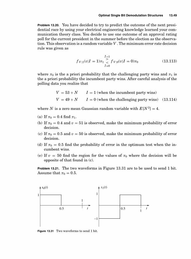
Optimal Single Bit Demodulation Structures 13.49
Problem 13.20. You have decided to try to predict the outcome of the next presi-dential race by using your electrical engineering knowledge learned your com-munication theory class. You decide to use one outcome of an approval ratingpoll for the current president in the summer before the election as the observa-tion. This observation is a random variable V . The minimum error rate decisionrule was given as
f V |1(v|I = 1)π1
I =1><
I =0
f V |0(v|I = 0)π0 (13.113)
where π0 is the a priori probability that the challenging party wins and π1 isthe a priori probability the incumbent party wins. After careful analysis of thepolling data you realize that
V = 53 + N I = 1 (when the incumbent party wins)
V = 49 + N I = 0 (when the challenging party wins) (13.114)
where N is a zero mean Gaussian random variable with E[N 2] = 4.
(a) If π0 = 0.4 find π1.
(b) If π0 = 0.4 and v = 51 is observed, make the minimum probability of errordecision.
(c) If π0 = 0.5 and v = 50 is observed, make the minimum probability of errordecision.
(d) If π0 = 0.5 find the probability of error in the optimum test when the in-cumbent wins.
(e) If v = 50 find the region for the values of π0 where the decision will beopposite of that found in (c).
Problem 13.21. The two waveforms in Figure 13.31 are to be used to send 1 bit.Assume that π0 = 0.5.
x0(t) x1(t)
1 1
t t
−1
1
10.50.5
Figure 13.31 Two waveforms to send 1 bit.

13.50 Chapter Thirteen
(a) Compute E0 and E1.
(b) Specify the optimum demodulator structure. Clearly specify any thresholdtest, filter impulse responses, and/or sample times.
(c) Compute the Euclidean distance between x0(t) and x1(t).
Problem 13.22. Using the Rayleigh energy theorem show that
[ρ10] = [∫∞−∞ X1(f )X ∗
0(f )df]
√E1 E0
(13.115)
Problem 13.23. In a manufacturing assembly line the error in placing an objectin a test fixture is modeled as a random variable, V I . If the robot is properlycalibrated then the error is well modeled as
f V I (v|C) =⎧⎨⎩
12
−1 ≤ v ≤ 1
0 elsewhere(13.116)
If the robot is not calibrated then the error is well modeled as
f V I (v|N C) = 1√2π
exp[−v2
2
](13.117)
Assume the robot is calibrated roughly 75% of the time (πC = 0.75).Hint: Since Eq. (13.116) is not a Gaussian PDF, a little thought will be needed
to generalize the results of this chapter to answer the questions.
(a) If you observe a Vi = v give a decision algorithm based on the value of v thatwould give the minimum probability of error in determining if the systemwas uncalibrated.
(b) If the robot is calibrated only 25% of the time the decision algorithm willchange. Precisely define the new decision algorithm for πC = 0.25. Give theintuition of why the decision algorithm has changed so dramatically.
13.9 Example Solutions
Problem 13.10.
(a) The plot of the bandpass signal corresponding to x0(t) is shown inFigure 13.32.
(b) The block diagram of the optimum demodulator is exactly as given in thetext (see Figure 13.33).
(c) Recall for an optimal demodulator of a binary signal set that the BEP isgiven as
PB (E) = 12
erfc
⎛⎝√
�E (1, 0)4N0
⎞⎠ (13.118)

Optimal Single Bit Demodulation Structures 13.51
−1.5
−1
−0.5
0
0.5
1
1.5
−0.2 0 0.2 0.4 0.6 0.8 1.21
x 0(t
)
Normalized Time, t/Tp
Figure 13.32 The bandpass signal corresponding to x0(t).
The Euclidean square distance for this signal set is
�E (1, 0) =∫ Tp
0|x1(t) − x0(t)|2dt (13.119)
= 2Eb − 2Eb
Tp
∫ Tp
0{
exp(
jπt
2Tp− j θ)}
dt (13.120)
= 2Eb − 2Eb
Tp{
exp(− j θ )∫ Tp
0exp(
jπt
2Tp
)dt}
(13.121)
= 2Eb − 2Eb{
exp(− j θ )(
sin(π/2)π/2
− cos(π/2) − 1π/2
)}(13.122)
= 2Eb − 4Eb
π{exp(− j θ )(1 + j )} (13.123)
Re[•]
argmax
Re[•]
Yz(t)
x0(Tp − t)
x1(Tp − t)
Tp
TpÎ
Figure 13.33 Demodulator block diagram.

13.52 Chapter Thirteen
The maximum Euclidean square distance is achieved for θ = −3π/4. Notethis best performance is
�(1, 0) = 2Eb
(1 + 2
√2
π
)= 3.8Eb < 4Eb (13.124)
so that the performance is worse than BPSK but better than the best BFSKsignaling scheme as introduced in class.
(d)
Gx0 (f ) = EbTp(sinc ( f Tp − π/8))2 (13.125)
Gx1 (f ) = EbTp(sinc ( f Tp + π/8))2 (13.126)
DXz(f ) = 12
(Gx0 (f ) + Gx1 (f )
)(13.127)
This energy spectrum is given in Figure 13.34. Examining this figure givesB3 = 0.88.
Problem 13.13. This signaling scheme is known as fast frequency hopping.
−5 −4 −3 −2 −1 0 1 2 3 4 5−50
−45
−40
−35
−30
−25
−20
−15
−10
−5
0
5
Normalized Frequency, f Tp
Dx z
(f),
dB
Figure 13.34 The average energy spectral density. π0 = π1 = 0.5.

Optimal Single Bit Demodulation Structures 13.53
(a) This modulation has the form Xi(t) = diu(t). Hence only one filter is neededand this is given as
Q =∫
Yz(t)u∗(t)dt (13.128)
=∫ Tp
2
0Yz(t)
√Eb
Tpexp[− j 2π f1t]dt +
∫ Tp
Tp2
Yz(t)
√Eb
Tpexp[− j 2π f 2t]dt
(13.129)
The ML decision metrics can be formulated as
Ei = |di|2 Eu = |di|2 Eb (13.130)
T 0 = [d ∗0 Q] − |d0|2 Eb
2(13.131)
T 1 = [d ∗1 Q] − |d1|2 Eb
2(13.132)
(b)
PB (E) = 12
erfc
⎡⎣√
�E (1, 0)4N0
⎤⎦ (13.133)
where �E (1, 0) = |d0 − d1|2 Eb (13.134)
(c) Since d0 = 1 and d0 = −1 this produces �E (1, 0) = 4Eb.
(d) Only point of possible discontinuity is at t = Tp/2.
2π f1Tp
2= 2π f 2
Tp
2(13.135)
2π f1Tp
2= 2π f 2
Tp
2+ 2πn where n is an integer (13.136)
f 2 = f1 + 2nTp
(13.137)
(e) The average energy spectrum is given as
Dxz(f ) = 12
(GX0 (f ) + GX1 (f )) (13.138)
Since Xi(t) = diu(t), the individual energy spectrums are given as
GX0 (f ) = |X0(f )|2 = |d0|2|U (f )|2 = |U (f )|2 = GX1 (f ) (13.139)

13.54 Chapter Thirteen
Note that u(t) = u1(t) + u2(t) where
u1(t) =
⎧⎪⎨⎪⎩√
Eb
Tpexp[ j 2π f1t] 0 ≤ t ≤ Tp/2
0 elsewhere
(13.140)
and
u2(t) =
⎧⎪⎨⎪⎩√
Eb
Tpexp[ j 2π f1t] Tp/2 ≤ t ≤ Tp
0 elsewhere
(13.141)
Taking the Fourier transform gives
U1(f ) =√EbTp exp[− j
π f Tp
2
]sinc(
( f − f1)Tp
2
)(13.142)
and
U2(f ) =√EbTp exp[− j
3π f Tp
2
]sinc(
( f − f 2)Tp
2
)(13.143)
Finally
|U (f )|2 = |U1(f ) + U2(f )|2 = Dxz(f ) (13.144)
See Matlab code and plot in Figure 13.35.
%% Generating the spectrum of FH% Author: M. Fitz% Last modified: 1/28/04%close allclear allnumpts=2048;f_1=2;f_2=-2;freq=linspace(-4,4, numpts+1);g_pr=zeros(1,numpts+1);dum1=exp(-j*pi*freq/2).*sinc(freq-f_1*ones(1,numpts+1));dum2=exp(-j*3*pi*freq/2).*sinc(freq-f_2*ones(1,numpts+1));g_pr=(dum1+dum2).*conj(dum1+dum2);g_prdb=10*log10(g_pr);figure(1)plot(freq,g_prdb)axis([-4 4 -50 5])xlabel('Normalized frequency, fT_p')ylabel('Normalized energy spectrum per bit')hold off

Optimal Single Bit Demodulation Structures 13.55
−4 −3 −2 −1 0 1 2 3 4−50
−45
−40
−35
−30
−25
−20
−15
−10
−5
0
5
Normalized Frequency, fTp
Nor
mal
ized
Ene
rgy
Spec
trum
per
bit
Figure 13.35 Spectrum of a frequency hopped signal.
13.10 Miniprojects
Goal: To give exposure
■ to a small scope engineering design problem in communications.■ to the dynamics of working with a team.■ to the importance of engineering communication skills (in this case oral pre-
sentations).
Presentation: The forum will be similar to a design review at a company(only much shorter). The presentation will be of 5 minutes in length with anoverview of the given problem and solution. The presentation will be followedby questions from the audience (your classmates and the professor). Each teammember should be prepared to give the presentation.
13.10.1 Project 1
Project Goals: This project will design a signal set to meet a typical spectralemissions mask and compute the probability of error for both bandpass andbaseband matched filtering in the presence of sample time error to show theadvantages of processing signals at baseband.
Design a real valued pulse shape, u(t), that can be used with binary pulseamplitude modulation having the bandpass form
xc0(t) = u(t)√
2 cos(2π f ct) xc1(t) = −u(t)√
2 cos(2π f ct)

13.56 Chapter Thirteen
0
0 100 200 300 400Frequency Offset, kHz
500 600 700 800
Rel
ativ
e E
mis
sion
s L
evel
, dB
Figure 13.36 Spectral emissions mask.
that will meet the spectral emissions mask given in Figure 13.36 but the pulsemust not extend for longer than 40 µs in time. The carrier frequency is 1 MHz.This spectral emissions mask is the one used for Global System for Mobile com-munications (GSM) handsets. GSM is a second generation cellular telephonystandard. So this problem is one of great practical interest.
We have discussed one type of demodulator structures for bandpass signals;baseband matchd filters. This structure match filters to the bandpass signalafter creating the complex envelope of the received signal (see Figure 13.37).It is also possible to build a matched filter to the bandpass signal itself (h(t) =x1c(Tp − t) − x0c(Tp − t))
+− I
2cos(2πfct)
u(Tp − t)LPFyc(t)
t = Tp
Figure 13.37 The baseband demodulator for binary pulse amplitude modulation.

Optimal Single Bit Demodulation Structures 13.57
(a) Derive the form for and plot the output of the bandpass matched filter forall time when xc(t) = u(t)
√2 cos(2π f ct).
(b) Derive the form for and plot the output of the baseband matched filter whenxc(t) = u(t)
√2 cos(2π f ct).
(c) Compute the Eb/N0 required to produce a 10−5 error probability for theoptimum demodulator.
(d) If the bandpass matched filter is sampled at Tp + 2 × 10⁻⁷ instead of Tpcompute the Eb/N0 required to produce a 10−5 error probability.
(e) If the baseband matched filter is sampled at Tp + 2 × 10⁻⁷ instead of Tpcompute the Eb/N0 required to produce a 10−5 error probability.
(f) How big would the timing error have to be for the baseband matched filterto achieve the same answer as in (d)?
13.10.2 Project 2
Project Goals: Engage in an implementation of an optimum demodulator ofa binary signal set.
Consider baseband binary signal set (with sample frequency f s = 22,050 Hz)and the received bandpass signal ( f c = 3500 Hz) given in sbproj2data.mat.
(a) Plot the two baseband signals and determine the bit rate, Wb.
(b) Sketch a block diagram of the optimum demodulator for these two signals.
(c) Make the optimum bit decision and compute all the sufficient statisticsof the demodulation. Hint: If implementing the demodulator at basebandmake sure to account for the impact of the lowpass filters in the I/Q down-converter on the possible baseband signals.

This page intentionally left blank

Chapter
14Transmitting More Than One Bit
People who buy communication systems rarely want to only transmit 1 bit. Con-sequently, there is a practical need to generalize the results from the previouschapter to the transmission of multiple bits. The problem considered here isthat we transmit Kb bits by selecting one of M = 2Kb waveforms. In the litera-ture this is often denoted M-ary digital communications. The demodulator hasthe task of deciding which of these waveforms was sent in the presence of anadditive noise. This chapter will consider a variety of problems associated withtransmitting more than 1 bit.
14.1 A Reformulation for 1 Bit Transmission
The optimum demodulator can be reformulated in several ways. Many of thesereformulations give insight for receiver structures we will consider in the se-quel. Recall from Chapter 13 that the MLBD, when Yz(t) = yz(t) is observed,has the form
vI (Tp) = [∫ ∞
−∞yz(τ )(x∗
1(τ ) − x∗0(τ ))dτ
] I =1><
I =0
E1 − E0
2(14.1)
Rearranging Eq. (14.1) gives
[∫ ∞
−∞yz(τ )x∗
1(τ )dτ
]− E1
2
I =1><
I =0
[∫ ∞
−∞yz(τ )x∗
0(τ )dτ
]− E0
2(14.2)
The form of the MLBD in Eq. (14.2) which forms a decision statistic for eachpossible signal by computing the output of a matched filter to that transmit-ted signal and adding an energy correction term will frequently appear in thesequel. In fact, to simplify the discussion the following definition is useful.
14.1
Copyright © 2007 by The McGraw-Hill Companies. Click here for terms of use.

14.2 Chapter Fourteen
Definition 14.1 The maximum likelihood metric for I = i is
T i = [∫ ∞
−∞yz(τ )x∗
i (τ )dτ
]− Ei
2(14.3)
Using this definition allows a reformulation of the MLBD as
T 1
I =1><
I =0
T 0 (14.4)
Equation (14.4) gives a particularly insightful form of the decision process: formthe maximum likelihood metric for each bit value and choose to decode the bitvalue corresponding to the largest metric.
The MAPBD can similarly take other useful forms. Multiplying both sidesof Eq. (14.2) by 2/N0 and taking the exponential gives another form for theMLBD, i.e.,
exp[
2N0
[∫ ∞
−∞yz(τ )x∗
1(τ )dτ
]− E1
N0
] I =1><
I =0
exp[
2N0
[∫ ∞
−∞yz(τ )x∗
0(τ )dτ
]− E0
N0
](14.5)
The justification of why the constant term is 2/N0 is provided in a book on detec-tion theory [Poo88]. Using the maximum likelihood metric the MLBD simplifiesto
exp[
2T 1
N0
]π1
I =1><
I =0
exp[
2T 0
N0
]π0 (14.6)
The generalization to unequal priors has the MAPBD taking the form
exp[
2N0
[∫ ∞
−∞yz(τ )x∗
1(τ )dτ
]− E1
N0
]π1
I =1><
I =0
exp[
2T 1
N0
] I =1><
I =0
exp[
2T 0
N0
](14.7)
In fact, this demodulator structure can be viewed as being equivalent to com-puting the APP for each of the two possible bits given the receiver input andthen selecting the bit value that corresponds to this maximum, i.e.,
exp[
2T 1N0
]π1
K= P (I = 1|yz(t))
I =1><
I =0
P (I = 0|yz(t)) =exp[
2T 0N0
]π0
K(14.8)
where yz(t) is the observed receiver input and K is a constant that is not afunction of I . Forms for the optimal detector given in Eq. (14.5) and Eq. (14.7)will be used often in the sequel to form optimum detectors in some special cases.

Transmitting More Than One Bit 14.3
14.2 Optimum Demodulation
Now we want to consider the digital communication system design problem oftransmitting more than one bit of information. In the sequel, Kb shall denotethe number of bits to be transmitted and the bit sequence is denoted
�I = [I (1) I (2) . . . I (Kb)]T (14.9)
where I (k) take values 0,1. For simplicity of notation a particular sequenceof bits can be designated by the numeric value the bits represent, i.e., �I = i,i ∈ {0, . . . , M − 1} where M = 2Kb. To represent the M values the bit sequencecan take, M different analog waveforms should be available for transmission.Denote by xi(t), i ∈ {0, . . . , M − 1} as the waveform transmitted when �I = iis to be transmitted. Here again we will assume the analog waveforms havesupport on t ∈ [0, Tp]. Given this problem formulation we want to extend theresults obtained in the previous chapter. It is worth noting that this problemformulation gives a bit rate of Wb = Kb/Tp bits per second. The average energyper bit is given as
Eb = 1Kb
M−1∑i=0
πi Ei (14.10)
where again Ei is the energy of waveform xi(t).
EXAMPLE 14.1Consider the case of Kb = 3, the bits and the words are enumerated as
I (1) I (2) I (3) i0 0 0 00 0 1 10 1 0 20 1 1 31 0 0 41 0 1 51 1 0 61 1 1 7
EXAMPLE 14.2Here we consider a modulation known as pulse width modulation with Kb = 2. Thismodulation embeds information in the width of the pulse that is transmitted. This is apopular baseband modulation in certain applications where positive logic level signals

14.4 Chapter Fourteen
are desired in the transmitter. The transmitted signals are given as
x0(t) =
⎧⎨⎩√
32Eb10Tp
0 ≤ t ≤ Tp/4
0 elsewherex1(t) =
⎧⎨⎩√
32Eb10Tp
0 ≤ t ≤ Tp/2
0 elsewhere(14.11)
x2(t) =
⎧⎨⎩√
32Eb10Tp
0 ≤ t ≤ 3Tp/4
0 elsewherex3(t) =
⎧⎨⎩√
32Eb10Tp
0 ≤ t ≤ Tp
0 elsewhere(14.12)
A student exercise worth completing is to show that energy per bit for this signal setis Eb.
14.2.1 Optimum Word Demodulation Receivers
A first receiver to be considered is the maximum a posteriori word demodulator(MAPWD). This MAPWD can again be shown to be the minimum word errorprobability receiver using Bayes detection theory [Leh86, Web87]. A straight-forward generalization of Eq. (14.8) leads to
�I = arg maxi∈{0,...,M−1}
P ( �I = i|yz(t)) (14.13)
where the arg max notation refers to the particular binary word that has themaximum APP. This is the obvious generalization of binary MAP detection tothe M-ary decision problem. Using the results of the previous section this MAPdecoding rule becomes
�I = arg maxi∈{0,...,M−1}
exp[
2N0
[∫ ∞
−∞yz(τ )x∗
i (τ )dτ
]− Ei
N0
]πi
= arg maxi∈{0,...,M−1}
exp[
2N0
[vi(Tp)] − Ei
N0
]πi (14.14)
= arg maxi∈{0,...,M−1}
exp[
2T i
N0
]πi (14.15)
where
vi(t) =∫ ∞
−∞yz(τ )x∗
i (Tp − t + τ )dτ (14.16)
is denoted the ith matched filter output and
Ei =∫ ∞
−∞|xi(t)|2dt (14.17)
is the energy of the ith analog waveform. The ith matched filter output whensampled at t = Tp again will give a correlation of the received signal with theith possible transmitted signal. Here T i represents the maximum likelihood

Transmitting More Than One Bit 14.5
MF x0(t)
E0/2
E1/2
−
+
p0
p1
Tp
−
+
Tp
−
+
Tp
…
EM-1/2
MF xM-1(t)
MF x1(t)ChooseLargest
2N0
2N0
Re[•]
Re[•]
Re[•]
Σ
Σ
Σ
exp(•)
exp(•)→I
Yz(t)
2N0
exp(•)
pM-1
Figure 14.1 The block diagram for the M-ary MAP demodulator.
metric for the word �I = i. For future use it is important to reemphasize that
exp[
2T i
N0
]πi = exp
[2
N0[vi(Tp)] − Ei
N0
]πi = K P ( �I = i|yz(t)) (14.18)
where K is a constant that is not a function of �I . The block diagram for theoptimum MAPWD is shown in Figure 14.1.
The demodulator in the case of equal priors, i.e., πi = 1/M, ∀i, can be greatlysimplified. We will denote this demodulator as the maximum likelihood worddemodulator (MLWD). Since all terms have an equal πi this common term canbe canceled from each term in the decision rule and since the ln(•) function ismonotonic the MLWD is given as
�I = arg maxi∈{0,...,M−1}
[vi(Tp)] − Ei
2
= arg maxi∈{0,...,M−1}
T i (14.19)
The maximum likelihood metric is computed for each of the possible transmittedsignals. Decoding is accomplished by selecting the binary word associated withthe largest maximum likelihood metric. The block diagram for the optimumMLWD is shown in Figure 14.2.

14.6 Chapter Fourteen
MF x0(t)
E0/2
−
+
Tp
Tp
−
+
−
+
Tp
MF xM-1(t)
ChooseLargest
T0
T1
TM-1
Yz t( )
Re[•]
Re[•]
Σ
Σ
Σ
MF x1(t) Re[•]
E1/2
EM-1/2
→I
…
Figure 14.2 The block diagram for the MLWD demodulator.
EXAMPLE 14.3This example returns to the 4-ary example first introduced in Example 12.1. Since thepossible transmitted signals are real, the four matched filter outputs are given as
v0(Tp) =∫ Tp
0sin
(4πτ
Tp
)yz(τ )dτ v1(Tp) =
∫ Tp
0yz(τ )dτ
v2(Tp) = −∫ Tp
0sin
(πτ
Tp
)yz(τ )dτ
v3(Tp) =∫ Tp/2
0
2τ
Tpyz(τ )dτ +
∫ Tp
Tp/2
(2 − 2τ
Tp
)yz(τ )dτ (14.20)
The energy of each of the transmitted signals is given as
E0 = Tp/2 E1 = Tp E2 = Tp/2 E3 = Tp/3 (14.21)
The maximum likelihood metrics for this modulation are given as
T 0 = [v0(Tp)] − Tp/2 T 1 = [v1(Tp)] − Tp
T 2 = [v2(Tp)] − Tp/2 T 3 = [v3(Tp)] − Tp/3 (14.22)

Transmitting More Than One Bit 14.7
EXAMPLE 14.4Returning to the pulse width modulation first introduced in Example 14.2, the fourmatched filter outputs are given as
v0(Tp) =√
32Eb
10Tp
∫ Tp/4
0yz(τ )dτ v1(Tp) =
√32Eb
10Tp
∫ Tp/2
0yz(τ )dτ
v2(Tp) =√
32Eb
10Tp
∫ 3Tp/4
0yz(τ )dτ v3(Tp) =
√32Eb
10Tp
∫ Tp
0yz(τ )dτ (14.23)
The energy of each of the transmitted signals is given as
E0 = 8Eb
10E1 = 16Eb
10E2 = 24Eb
10E3 = 32Eb
10(14.24)
The maximum likelihood metrics for this modulation are given as
T 0 =√
32Eb
10Tp
∫ Tp/4
0yI (τ )dτ − 4Eb
10T 1 =√
32Eb
10Tp
∫ Tp/2
0yI (τ )dτ − 8Eb
10
T 2 =√
32Eb
10Tp
∫ 3Tp/4
0yI (τ )dτ − 12Eb
10T 3 =√
32Eb
10Tp
∫ Tp
0yI (τ )dτ − 16Eb
10
(14.25)
The important thing to notice for both MAPWD and MLWD is that the optimaldemodulator complexity increases exponentially with the number of bits trans-mitted. The number of matched filters required in each demodulator is M = 2Kb,consequently the complexity of these demodulation schemes is O(2Kb). The no-tation O(x) implies the complexity of the algorithm is proportional to x, i.e., aconstant times x. This complexity is obviously unacceptable if large files of dataare to be transmitted. To make data communications practical, ways will haveto be developed that make the complexity linear in the number of bits sent,i.e., O(Kb). This chapter will continue to look at M-ary signaling schemes asthey often are used in practice (in conjunction with other complexity reductiontechniques) to achieve either lower error rates or higher bandwidth efficiency.
14.2.2 Analysis of Demodulation Fidelity
The analysis of the fidelity of the message reconstruction in an M-ary demod-ulator is much more complicated than that of the binary detector but many ofthe ideas are similar. Two important quantities should be related at this point:the energy per symbol and the energy per bit. The average symbol energy isdenoted Es and this is given as
Es =M−1∑i=0
Eiπi (14.26)

14.8 Chapter Fourteen
Es represents the average energy transmitted to communicate the Kb bits. Thecase of equal priors reduces to
Es = 1M
M−1∑i=0
Ei (14.27)
The average energy per bit is then given as
Eb = Es
Kb(14.28)
Communication engineers frequently parametrize fidelity of demodulation withboth Es and Eb.
EXAMPLE 14.5Returning again to the pulse width modulation introduced in Example 14.2 we have
Eb = E0 + E1 + E2 + E3
8=(
8Eb
80+ 16Eb
80+ 24Eb
80+ 32Eb
80
)(14.29)
We again start the process of understanding the fidelity of demodulation bycharacterizing the likelihood metrics.
Likelihood Metrics
The likelihood metrics, T i, i ∈ {0, . . . , M − 1} are matched filter outputs withan energy correction term. Conditioned on the transmitted signal the likeli-hood metrics are Gaussian random variables. For instance, if xj (t) is assumedtransmitted then denote the ith conditional likelihood metric as
Ti| j = [∫ ∞
−∞Yz(t)x∗
i (t)dt]
− Ei
2
= [∫ ∞
−∞xj (t)x∗
i (t)dt]
+ N (i)I − Ei
2(14.30)
where N (i)I is a real zero mean Gaussian random variable given as
N (i)I =
[∫ ∞
−∞Wz(t)x∗
i (t)dt]
(14.31)
with
var(N (i)I ) = Ei N0
2. (14.32)
It should be noted that
Ti| j = [ρ j i√
Ei E j ] − Ei
2+ N (i)
I
T j | j = E j
2+ N ( j )
I (14.33)

Transmitting More Than One Bit 14.9
Finally, if two conditional likelihood metrics, Ti| j and T k| j are consideredjointly, they will be jointly Gaussian random variables with a correlation co-efficient of (see Problem 14.14)
ρ = E[N (i)
I N (k)I
]N02
√Ei Ek
= [ρik] (14.34)
This correlation between the matched filter outputs will be explored in moredepth in the homework.
Probability of Word Error
The probability of making a demodulation error is denoted the word error prob-ability, PW (E). This probability can be written via total probability as
PW (E) =M−1∑j =0
P (�I �= j | �I = j )π j (14.35)
When the priors are unequal the nonlinear nature of MAPWD in Eq. (14.14)makes the computation of P (�I �= j | �I = j ) very difficult. Not many results existin the literature discussing PW (E) calculations for MAPWD.
The case of equal priors has a demodulator with a more exploitable structure.For MLWD the word error probability is
PW (E) = 1M
M−1∑j =0
P (�I �= j | �I = j ) (14.36)
The conditional probability of word error is given as
P (�I �= j | �I = j ) = P(
maxj �=i
T i > T j
∣∣∣ �I = j)
= P(
maxj �=i
Ti| j > T j | j
)
= P
⎛⎜⎜⎝
M−1⋃i=0j �=i
{Ti| j > T j | j }
⎞⎟⎟⎠ (14.37)
In general, the probability in Eq. (14.37) is quite tough to compute. While eachof the Ti| j , i = 1, M is a Gaussian random variable, computing the distributionof the maximum of correlated Gaussian random variables is nontrivial. For asignificant number of modulations with small M the probability in Eq. (14.37)is computable with a reasonable amount of work on a computer. Some of theseexamples will be explored in the sequel and in homework problems. For a gen-eral modulation and large M the problem is much tougher. One special case

14.10 Chapter Fourteen
where a general result is available is the case of an orthogonal modulation, i.e.,ρi j = 0, ∀i �= j . Error rate analysis for an orthogonal signal set is explored inthe homework.
14.2.3 Union Bound
A common upperbound on the probability in Eq. (14.37) has found great utilityin the analysis of communication systems. This so-called union bound is simplystated in general form as
P
(N⋃
i=1
Ai
)≤
N∑i=1
P ( Ai) (14.38)
where Ai are arbitrary events. The idea of the union bound is simply understoodif one considers the Venn diagram of Figure 14.3. Consider the probability ofeach event, Ai to be proportional to the area in the Venn diagram. The unionbound given in Eq. (14.38) counts the area in A1
⋂A2, A1
⋂A3, and A2
⋂A3
twice and the area of A1⋂
A2⋂
A3 three times. The union bound is satisfiedwith equality if the events are disjoint.
The union bound can now be used to upperbound the word error probabilityin an M-ary optimum word demodulator. Using the union bound in Eq. (14.37)gives
P (�I �= j | �I = j ) = P
⎛⎜⎜⎝
M−1⋃i=0j �=i
{Ti| j > T j | j }
⎞⎟⎟⎠
≤M−1∑
i=0j �=i
P (Ti| j > T j | j ) (14.39)
P (Ti| j > T j | j ) is the probability that the ith maximum likelihood metric forthe transmitted signal is greater than the maximum likelihood metric corre-sponding to the actual transmitted signal. This probability is often denoted thepairwise error probability (PWEP).
A1
A2
A3
A3 ∩ A1
A2 ∩ A1
A1∩ A2 ∩ A3
A2 ∩ A3
Figure 14.3 A Venn diagram to explainthe union bound.

Transmitting More Than One Bit 14.11
The PWEP has a form readily analyzed. It should first be noted that thePWEP is exactly the same error rate computation that was done in Chapter 13for binary modulations. This derivation is repeated here in its more generalform to give another perspective on the problem. Recall the form for the decisionmetrics are
Ti| j = [ρ j i√
Ei E j ] − Ei
2+ N (i)
I
T j | j = E j
2+ N ( j )
I (14.40)
Consequently, the PWEP is given as
P (Ti| j > T j | j ) = P(
[ρ j i√
Ei E j ] − Ei
2+ N (i)
I >E j
2+ N ( j )
I
)
= P(
Nij >Ei + E j
2− [ρ j i
√Ei E j ]
)(14.41)
= P(
Nij >�E (i, j )
2
)(14.42)
where Nij = N (i)I − N ( j )
I . Since Nij is a zero mean Gaussian random variablethe PWEP is simply expressed as the tail probability of a Gaussian randomvariable. Since
Nij = [∫ ∞
−∞Wz(t)[x∗
i (t) − x∗j (t)]dt
](14.43)
the variance is given as
var(Nij ) = N0
2[Ei + E j − 2[ρ j i
√Ei E j ]] = N0�E (i, j )
2(14.44)
Using this variance in Eq. (14.41) gives
P (Ti| j > T j | j ) = 12
erfc
⎛⎝√
Ei + E j − 2[ρ j i√
Ei E j ]4N0
⎞⎠
= 12
erfc
⎛⎝√
�E (i, j )4N0
⎞⎠ (14.45)
where again
�E (i, j ) =∫ ∞
−∞|xj (t) − xi(t)|2dt (14.46)
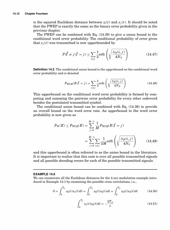
14.12 Chapter Fourteen
is the squared Euclidean distance between xi(t) and xj (t). It should be notedthat the PWEP is exactly the same as the binary error probability given in theprevious chapter.
The PWEP can be combined with Eq. (14.39) to give a union bound to theconditional word error probability. The conditional probability of error giventhat xj (t) was transmitted is now upperbounded by
P (�I �= j | �I = j ) ≤∑i �= j
12
erfc
⎛⎝√
�E (i, j )4N0
⎞⎠ (14.47)
Definition 14.2 The conditional union bound is the upperbound on the conditional worderror probability and is denoted
PWUB(E| �I = j ) =∑i �= j
12
erfc
(√�E (i, j )
4N0
)(14.48)
This upperbound on the conditional word error probability is formed by com-puting and summing the pairwise error probability for every other codewordbesides the postulated transmitted symbol.
The conditional union bound can be combined with Eq. (14.36) to providean overall bound on the word error rate. An upperbound to the word errorprobability is now given as
PW (E) ≤ PWUB(E) =M−1∑j =0
1M
PWUB(E| �I = j )
=M−1∑j =0
∑i �= j
12M
erfc
⎛⎝√
�E (i, j )4N0
⎞⎠ (14.49)
and this upperbound is often referred to as the union bound in the literature.It is important to realize that this sum is over all possible transmitted signalsand all possible decoding errors for each of the possible transmitted signals.
EXAMPLE 14.6We can enumerate all the Euclidean distances for the 4-ary modulation example intro-duced in Example 12.1 by examining the possible cross correlations, i.e.,
0 =∫ Tp
0x0(t)x1(t)dt =
∫ Tp
0x0(t)x2(t)dt =
∫ Tp
0x0(t)x3(t)dt (14.50)
∫ Tp
0x1(t)x2(t)dt = −2Tp
π(14.51)

Transmitting More Than One Bit 14.13
∫ Tp
0x1(t)x3(t)dt = Tp
2(14.52)
∫ Tp
0x2(t)x3(t)dt = −4Tp
π2(14.53)
This results in an enumeration of the possible Euclidean square distances that is detailedin the following table
�E (i, j )
�I = i
�I = j 0 1 2 3
0 0 3Tp2 Tp
5Tp6
1 3Tp2 0
( 32 + 4
π
)Tp
Tp3
2 Tp( 3
2 + 4π
)Tp 0
( 56 + 8
π2
)Tp
3 5Tp6
Tp3
( 56 + 8
π2
)Tp 0
This enumeration of the squared Euclidean distances between all pairs of words enablethe union bound to be computed for this signal set.
EXAMPLE 14.7We can enumerate all the Euclidean distances for the pulse width modulation firstintroduced in Example 14.2 in a table
�E (i, j )
�I = i
�I = j 0 1 2 3
0 0 8Eb10
16Eb10
24Eb10
1 8Eb10 0 8Eb
1016Eb
10
2 16Eb10
8Eb10 0 8Eb
10
3 24Eb10
16Eb10
8Eb10 0
This enumeration of the squared Euclidean distances between all pairs of words enablethe union bound to be computed for this signal set.

14.14 Chapter Fourteen
The important points resulting from the union bound are
1. Squared Euclidean distance is again an important quantity in understand-ing the fidelity of message reconstruction.
2. The conditional union bound and the union bound typically have the form
PWUB(E| �I = j ) =N j∑
k=1
Ad j (k)2
erfc
⎛⎝√
�E j (k)4N0
⎞⎠ (14.54)
PW (E) ≤ PWUB(E) =N∑
k=1
Ad (k)2M
erfc
⎛⎝√
�E (k)4N0
⎞⎠ (14.55)
where the sum enumerates the N j ≤ M − 1 and N ≤ M(M − 1)/2 possibledifferent squared Euclidean distances, �E j (k), k = 1, N j and �E (k), k =1, N , respectively. Note that Ad j (k) and Ad (k) are the number of signalpairs having a squared Euclidean distance between them of �E j (k) and�E (k), respectively. It should also be noted that
∑N j
k=1 Ad j (k) = M − 1 and∑Nk=1 Ad (k) = M(M−1). The combination of the enumeration of the squared
Euclidean distance, �E (k), and the number of signal pairs Ad (k) for eachdistance is often denoted the squared Euclidean distance spectrum weight.All sets of pairs {�E (k), Ad (k)}, k = 1, N is often denoted the squared Eu-clidean distance spectrum of a signal set. Similiarly, a conditional Euclideandistance spectrum can be defined.
EXAMPLE 14.8For pulse width modulation there are two unique conditional Euclidean distance spectra.For �I = 0 there are three terms in the conditional distance spectrum, i.e.,
N0 = 3 {�E0(k) Ad 0(k)} ∈[{
8Eb
10, 1
},
{16Eb
10, 1
},
{24Eb
10, 1
}](14.56)
and for �I = 1 there are two terms, i.e.,
N1 = 2 {�E0(k) Ad 0(k)} ∈[{
8Eb
10, 2
},
{16Eb
10, 1
}](14.57)
which implies, for example, that
PWUB(E| �I = 0) = 12
erfc
(√8Eb
40N0
)+ 1
2erfc
(√16Eb
40N0
)+ 1
2erfc
(√24Eb
40N0
)
(14.58)
Pulling all the conditional distance spectra together we have N = 3 with �E (1) =8Eb10 , �E (2) = 16Eb
10 , and �E (3) = 24Eb10 and Ad (1) = 6, Ad (2) = 4, and Ad (3) = 2.

Transmitting More Than One Bit 14.15
Consequently, the union bound is expressed as
PW (E) ≤ PWUB(E) = 34
erfc
(√8Eb
40N0
)+ 1
2erfc
(√16Eb
40N0
)+ 1
4erfc
(√24Eb
40N0
)
(14.59)
3. The bound is often dominated by the minimum squared Euclidean distanceof the signal set, �E (min), where
�E (min) = minj ∈{0,...,M−1}i∈{0,...,M−1}
i �= j
�E (i, j ) (14.60)
Since erfc(x) ∼ exp[−x2] it is usually the case that
erfc
⎛⎝√
�E (min)4N0
⎞⎠� erfc
⎛⎝√
�E (i, j )4N0
⎞⎠ ∀�E (i, j ) �= �E (min) (14.61)
4. The union bound is usually tight at high SNR. The bound over counts thecases when more than one maximum likelihood metric for a nontransmit-ted word is greater than the maximum likelihood metric for the transmittedword. At high SNR the probability of two or more metrics being greater thanthe true metric is very small. Consequently, the overbounding probability isvery small.
5. Using items 3 and 4 allows one to deduce that
PW (E) ≈ Ad (min)2M
erfc
⎛⎝√
�E (min)4N0
⎞⎠ (14.62)
is a good approximation to the true error rate at high SNR.
EXAMPLE 14.9For pulse width modulation a reasonable estimate of performance at high SNR is ex-pressed as
PW (E) = 34
erfc
(√8Eb
40N0
)(14.63)
Similarly, for the 4-ary modulation introduced in Example 12.1 a reasonable estimateof performance at high SNR is expressed as
PW (E) = 14
erfc
(√Tp
12N0
)(14.64)

14.16 Chapter Fourteen
A concept that arises often in error rate analysis is the concept of geometricuniformity [For91].
Definition 14.3 A geometrically uniform signal set is one in which the conditional dis-tance spectrum of each of the possible transmitted signals is the same.
The important characteristic of a geometrically uniform signal set is
PWUB(E| �I = 0) = PWUB(E| �I = j ) = PWUB(E) (14.65)
This characteristic implies that the number of terms in the union bound thatneeds to be considered reduces from M(M − 1) to M − 1 as only one transmittedcode word needs to be considered. Note that pulse width modulation consideredin Example 14.4 is not a geometrically uniform signal set, but x0(t) and x3(t)have the same conditional distance spectrum as do x1(t) and x2(t).
14.2.4 Signal Design
Signal design for optimizing the fidelity of message reconstruction of an M-ary modulation is typically implemented with a max-min approach. Since theminimum squared Euclidean distance will dominate the word error rate of anoptimum demodulator, the best signal design will happen when the minimumdistance between all pairs of the M signals is maximized. This is known as themax-min design criteria for digital communications. In general, signal designin digital communications is a complex endeavor with many open problems.
The spectral characteristics of an M-ary signal set can be characterized witha straightforward extension of the techniques used for binary signals. Recallfrom Eq. (12.8) that the average energy spectrum per bit for a transmittedsignal, Xz(t), where Kb bits are transmitted is
Dxz(f ) = E[Gxz(f )]Kb
(14.66)
The average here again is over random data bits that are being transmitted.
EXAMPLE 14.10The average energy spectrum per bit for pulse width modulation can be obtained byidentifying the energy spectrum for each of the possible transmitted waveforms. Forpulse width modulation this is given as
Gx0 (f ) = T 2p
16sinc( f Tp/4)2 Gx1 (f ) = T 2
p
4sinc( f Tp/2)2 (14.67)
Gx2 (f ) = 9T 2p
16sinc(3 f Tp/4)2 Gx3 (f ) = T 2
p sinc( f Tp)2
If the signals are equally likely then the average energy spectrum for pulse widthmodulation is given in Figure 14.4. Since Wb = 2/Tp and using the 3 dB bandwidth(BT ≈ 1/Tp) the spectral efficiency is ηB = 2 bits/s/Hz.

Transmitting More Than One Bit 14.17
−6 −4 −2 0 2 4 6−50
−45
−40
−35
−30
−25
−20
−15
−10
−5
0
Nor
mal
ized
Dx z
(f)/
(Tp2 )
, dB
Normalized Frequency, fTp
Figure 14.4 The average energy spectrum per bit for pulse width modulation.
14.3 Examples
This chapter is concluded by considering two obvious and important examples ofM-ary carrier modulated digital communication: M-ary frequency shift keying(MFSK) and M-ary phase shift keying (MPSK). In these examples it is assumedthat πi = 1/M, i ∈ {0, . . . , M − 1}.
14.3.1 M-ary FSK
MFSK modulation sends the word of information by transmitting a carrierpulse of one of M frequencies. This is an obvious simple signaling scheme andone used in many early modems. The signal set is given as
xi(t) =
⎧⎪⎪⎨⎪⎪⎩
√KbEb
Tpexp[ j 2π fd (2i − M + 1)t] 0 ≤ t ≤ Tp
0 otherwise
(14.68)

14.18 Chapter Fourteen
where fd is known as the frequency deviation. The frequency difference be-tween adjacent frequency pulses in the signal set is 2 fd . It is apparent thateach waveform in a MFSK signal set has equal energy that has here been setto Es = KbEb.
The matched filter impulse response is given as
hi(t) = x∗i (Tp − t) (14.69)
Since MFSK is an equal energy signal set the energy correction term is notneeded in the demodulator and the ML decision metrics are given as
T i = [∫ Tp
0Yz(t)x∗
i (t)dt]
=√
KbEb
Tp[∫ Tp
0Yz(t) exp[− j 2π fd (2i − M + 1)t]dt
]
i ∈ {0, . . . , M − 1} (14.70)
The MLWD demodulator is then given as
�I = arg maxi∈{0,...,M−1}
T i (14.71)
This optimum demodulator computes M matched filter outputs and then selectsas a word estimate the word value that corresponds to the largest real part ofall the matched filter outputs.
The word error rate performance of MFSK is a function of the frequencyspacing, 2 fd . Using the results from BFSK, i.e., (13.87), the pairwise squaredEuclidean distance is given as �E (i, j ) = 2KbEb(1 − sin(4π fd (i− j )Tp )
4π fd (i− j )Tp). Conse-
quently, for MFSK the placement of the tones is a bit more delicate problem.The union bound is given as
PWUB(E) =M−1∑n=1
M − nM
erfc
(√KbEb
2N0
(1 − sin(4π fd nTp)
4π fd nTp
))(14.72)
The selection of the frequency spacing, fd , becomes a tricky problem for M > 2as one needs to balance all the terms in the union bound to optimize the errorrate. The MFSK signal set is not in general a geometrically uniform signal set.
For the special case of [ρi j ] = 0 both the PW (E) can be easily computedand a simple form for the union bound results. This is known as orthogonalMFSK and is achieved if fd = n
4Tpwhere n is a positive integer. The closed
form probability of error expression for orthogonal MFSK is explored in thehomework and plotted in Figure 14.5 for M = 2, 4, 8, 16. The important thingto realize for MFSK is that for large enough Eb/N0, the PW (E) is monotonicallydecreasing with M. In fact, one can show that the error rate can be madearbitrarily small when Eb/N0 > ln(2) [Sha48]. Consequently, the performance

Transmitting More Than One Bit 14.19
10−2
10−3
10−4
10−5
10−6
10−1
100
0 8642 10
M = 2M = 4 PWEM = 4 UBM = 8 PWEM = 8 UBM = 16 PWEM = 16 UB
Eb/N0, dB
P W(E
)
Figure 14.5 The true PW (E) and the union bound for orthogonal MFSK.
of a digital communication system can be improved by transmitting more bitsor having more waveforms to choose from. This result is also counter normalengineering intuition. Shortly, we will show that this performance improvementis achieved only at the cost of an increase in the bandwidth of the signal. Theunion bound for orthogonal MFSK is
PW (E) ≤ M − 12
erfc
(√KbEb
2N0
)(14.73)
For [ρi j ] = 0 MFSK is a geometrically uniform signal set. Figure 14.5 also plotsthe union bound for MFSK. It is obvious that the union bound converges to thetrue error probability at high SNR. For the particular case of MFSK the boundis tight enough to be indiscernibly different on the graph for Eb/N0 > 6 dB.This characteristic for the union bound holds for most signal sets optimallydemodulated in the presence of an AWGN.
The average energy spectrum per bit is again used to characterize the spectralefficiency. Recall the average energy spectral density per bit is given for M-ary

14.20 Chapter Fourteen
modulations as
Dxz(f ) = 1Kb
M−1∑i=0
πiGxi (f ) (14.74)
Recall that the energy spectrum of the individual waveforms is given as
Gxi (f ) = KbEbTp
(sin(π( f − fd (2i − M + 1))Tp)
π( f − fd (2i − M + 1))Tp
)2
(14.75)
Recall that the minimum frequency separation needed to achieve an orthogonalmodulation is fd Tp = 0.25 and that by considering Eq. (14.74) and Eq. (14.75) itis obvious that the spectral content is growing proportional to BT = fd (2Kb+1).An example of each of the individual energy spectrums (dotted lines) and theaverage energy spectrum for 8FSK (solid line) is plotted in Figure 14.6. Thetransmission rate of MFSK is Wb = Kb/Tp. The spectral efficiency then is ap-proximately ηB = Kb/2Kb−1 and decreases with the number of bits transmittedor equivalently decreases with M. Conversely MFSK provides monotonicallyincreasing performance with M. Consequently, MFSK has found use in practicewhen lots of bandwidth is available and good performance is required.
−8 −6 −4 −2 0 2 4 6 8−50
−45
−40
−35
−30
−25
−20
−15
−10
−5
0
5
Normalized Frequency, fTp
Nor
mal
ized
Dx z
(f),
dB
Figure 14.6 For 8FSK the Gxi (f ) for i ∈ {0, . . . , 7} and Dxz (f ) for fd Tp = 0.25.

Transmitting More Than One Bit 14.21
The advantages of MFSK are summarized as
■ Very simple to generate. Simply gate one of M oscillators on depending onthe word to be sent.
■ Performance (error rate) improves monotonically with Kb. This is counterintuition as normal intuition would expect performance degrading with in-creasing Kb.
The disadvantages of MFSK are summarized as
■ The bandwidth increases exponentially with Kb, hence the spectral efficiencyof MFSK decreases with Kb.
■ Complexity increases exponentially with Kb.
An additional important point demonstrated by this example
■ Union bound is simple to compute and is a tight bound at moderate to highSNR.
14.3.2 M-ary PSK
MPSK modulation sends the word of information by transmitting a carrierpulse of one of M phases. This is an obvious simple signaling scheme and oneused in many modems. The form of the signal set is given as
xi(t) =
⎧⎪⎪⎨⎪⎪⎩
√KbEb
Tpexp[ j θ (i)] 0 ≤ t ≤ Tp
0 elsewhere
(14.76)
where θ (i) is a mapping from the information words into a phase. The phasesin MPSK are normally uniformly spaced around the unit circle in engineeringpractice. The mapping of information word values into phases is not unique.Two common mappings exist in communications practice: natural mapping,θN (i), and Gray mapping, θG(i) [Gra53]. Natural mapping assigns the phasesequentially with the binary numeric representation of the information word.Unfortunately, if natural mapping is used then words which map to adjacentphases and hence close Euclidean distances can have many bit differences.Gray coding is a technique mitigating the effects of word errors on the PB (E)by mapping of binary words into phases in a way to where adjacent phases areonly different in 1 bit. An example of the two mappings for M = 4 is shown inTable 14.1. Since natural mapping is straightforward to enumerate functionally,i.e.,
θN (i) = π(2i + 1)M
(14.77)

14.22 Chapter Fourteen
TABLE 14.1 The two most common M = 4 PSK mappings
�I I (1) I (2) θN (i) θG(i)
0 00 π4
π4
1 01 3π4
3π4
2 10 5π4
7π4
3 11 7π4
5π4
the remainder of this section will consider natural mapping exclusively. Thesequel will return to consider Gray mapping in more detail for QPSK.
Since MPSK is an equal energy signal set the energy correction term is notneeded in the demodulator and the ML decision metrics are given as
T i = [∫ Tp
0Yz(t)x∗
i (t)dt]
=√
KbEb
Tp[∫ Tp
0Yz(t) exp
[− j
π(2i + 1)M
]dt]
= [
exp[− j
π(2i + 1)M
]√KbEb
Tp
∫ Tp
0Yz(t)dt
]
= [exp[− j
π(2i + 1)M
]Q]
i ∈ {0, . . . , M − 1} (14.78)
where
Q =√
KbEb
Tp
∫ Tp
0Yz(t)dt (14.79)
is denoted the pulse shape matched filter output. The MLWD computes theoutput of one filter, Q, derotates this value by each of the possible transmittedphasors and picks the signal that gives the largest real value. This decisionrule is equivalent to picking the transmitted phase that is closest to the phaseof the pulse shape matched filter so that
�I = arg maxi∈{0,...,M−1}
T i = arg mini∈{0,...,M−1}
∣∣∣∣Qp − π(2i + 1)M
∣∣∣∣ (14.80)
where Qp = arg{Q}.Surprisingly this optimum demodulator has only one filter output to compute.
This filter output is then processed to produce the decision metric. The worddecision is then made on the basis of which of these metric is the largest. Thedecision rule reduces down to the establishing of decision regions in the complexplane for the pulse matched filter output Q. The decision regions for 4PSK areshown in Figure 14.7a. The fact that the optimum M-ary demodulator only hasone filter is due to the transmitted signal set having the form
xi(t) = diu(t) (14.81)

Transmitting More Than One Bit 14.23
QI
I = 1 ÆI = 0 Æ
I = 2 ÆI = 3 Æ
Figure 14.7a The decision regions for natural mapping 4PSK.
where
u(t) =
⎧⎪⎨⎪⎩√
KbEb
Tp0 ≤ t ≤ Tp
0 elsewhere
(14.82)
is the pulse shape. Modulations which have the form of Eq. (14.81) are oftendenoted linear modulations by communications engineers. Since linear mod-ulations greatly reduce the demodulator complexity they will be explored indetail in the sequel.
The resulting error rate of MPSK is a function of the phase spacing, 2πM . The
squared Euclidean distance is given as �E (i, j ) = 2KbEb(1−cos( 2π(i− j )M )). Note
since cosine is a periodic function, MPSK is a geometrically uniform signal set.The union bound for MPSK is given as
PW (E) ≤ 12
erfc
(√KbEb
N0
)+
M/2−1∑i=1
erfc
(√KbEb
2N0
[1 − cos
(2πiM
)])(14.83)
The MFSK signal set was not in general a geometrically uniform signal set buthere we see that the MPSK signal set is geometrically uniform when the phasesof the modulation symbols are uniformly distributed around the unit circle.
It is interesting to note that for MPSK the union bound can actually be tight-ened compared to the general result given in Eq. (14.83). This tightening of theunion bound is due to the property on the next page.

14.24 Chapter Fourteen
A B
C
Figure 14.7b An event that doesnot need to be considered in theunion bound computation.
Property 14.1 P ( A∪ B ∪ C) = P ( A∪ B ) if C ⊂ A∪ B .
This property implies that if the set C is a subset of the union of the sets A and Bthen C can be ignored in computing a union bound. For digital communicationsthis implies that if any pairwise error event is a subset of the union of two(or more) pairwise error probabilities then that pairwise error event does notneed to be considered in the union bound computation. This concept is shownin Figure 14.7b with a Venn diagram.
Since the MPSK signal set is geometrically uniform we can consider x0(t) to bethe transmitted signal without loss of generality. The pairwise error probabilityis then given as
{Ti|0 > T0|0} ={
[exp[− j
π(2i + 1)M
]Q]
> [exp[− j
π
M
]Q]}
={∣∣∣∣Qp − π(2i + 1)
M
∣∣∣∣ < ∣∣∣Qp − π
M
∣∣∣} (14.84)
This reduces to
{Ti|0 > T0|0} ={
π(i + 1)M
≤ Qp ≤ π(M + i + 1)M
}(14.85)
Given this form of the pairwise error probability it can be seen that
{T1|0 > T0|0} ∪ {TM−1|0 > T0|0} ={
2π
M≤ Qp ≤ 2π
}(14.86)
Consequently, for any i ∈ {2, . . . , M − 2}
{Ti|0 > T0|0} ⊂ {T1|0 > T0|0} ∪ {TM−1|0 > T0|0} (14.87)
This implies that a tighter union bound for MPSK than Eq. (14.83) is given as
PW (E) ≤ erfc
(√KbEb
2N0
[1 − cos
(2π
M
)])(14.88)

Transmitting More Than One Bit 14.25
This tightened union bound only includes the minimum squared Euclideandistance terms. For MPSK these two pairwise error probability terms includeall the possible ways an error can occur.
MPSK word error probability performance can be computed exactly. If weassume that xk(t) was transmitted, the conditional matched filter output isgiven as
Q = exp[
jπ(2k + 1)
M
]KbEb + Nz (14.89)
where Nz is a complex Gaussian noise with a variance of
var(Nz) = N0KbEb (14.90)
Considering the decision regions and the form of the conditional matched filteroutput, the probability of word error can be computed. This idea is explored inthe homework problems. The resulting probability of word error is plotted inFigure 14.8 for M = 2, 4, 8, 16. In contrast to MFSK the probability of error
10−1
10−2
10−3
10−4
10−5
100
101
0 5 10 15 20
M = 2M = 4 PWEM = 4 UBM = 8 PWEM = 8 UBM = 16 PWEM = 16 UB
Eb/N0, dB
P W(E
)
Figure 14.8 The true PW (E) and the union bound for MPSK.

14.26 Chapter Fourteen
increases with M for MPSK. The error rate degrades about 4 dB for each dou-bling of M. The union bound is also plotted in Figure 14.8 for M = 2, 4, 8, 16.The union bound is again asymptotically tight with moderate SNR. This againdemonstrates the utility of a union bound error rate analysis.
The average energy spectrum per bit is again used to characterize the spectralefficiency of MPSK. Recall the average energy spectral density per bit is givenfor M-ary modulations as
Dxz(f ) = 1Kb
M−1∑i=0
πiGxi (f ) (14.91)
Recall that the energy spectrum of the individual waveforms is given as
Gxi (f ) = KbEbTp
∣∣∣∣exp[
jπ(2i + 1)
M
]∣∣∣∣2(sin(π f Tp)
π f Tp
)2
= KbEbTp
(sin(π f Tp)
π f Tp
)2
(14.92)
The occupied bandwidth of MPSK, BT = 1/Tp, does not increase with M whilethe bit rate does increase with M, Wb = Kb/Tp to provide a spectral efficiency ofηB = Kb. Unfortunately, the error rate of MPSK modulation increases with in-creasing M. Consequently, MPSK modulations are of interest in practice whenthe available bandwidth is small and the SNR is large.
The advantages of MPSK are summarized as
■ Very simple to generate. Simply change the phase of an oscillator to one Mvalues depending on the word to be sent.
■ No increase in the bandwidth occupancy with increasing Kb. Consequently,spectral efficiency increases with Kb.
■ Demodulation complexity does not increase exponentially with Kb.
The disadvantages of MPSK are summarized as
■ Error rate increases monotonically with Kb.
Additional important points demonstrated by this example
■ The most general union bound is simple to compute and is a tight bound atmoderate to high SNR.
■ The demodulator structure of MPSK allows a tighter union bound to be com-puted by considering the overlap in the decision regions.
14.3.3 Discussion
This section introduced two example modulations to transmit Kb bits of infor-mation: MFSK and MPSK. MPSK has the advantage in being able to supplyan increasing spectral efficiency with Kb at the cost of requiring more Eb/N0

Transmitting More Than One Bit 14.27
0
2
4
6
8
10
−5 0 5 10 15 20
Upperbound
MPSK
MFSK
Spec
tral
Eff
icie
ncy,
ηB
Eb/N0, dB
Figure 14.9 A comparison of the spectral efficiency of MPSK and MFSK with the upperbound.
to achieve the same error rate. MFSK can provide improved error rate perfor-mance with Kb but at a cost of a loss of spectral efficiency. Also the decodingcomplexity of MPSK is significantly less than the decoding complexity of MFSK.As a final point it is worth comparing the spectral efficiency performance ofthese two modulations with the upperbounds provided by information theory(see Section 12.3). As before we will denote reliable communication as beingan error rate of 10−5. The operating points of MFSK and MPSK and the up-perbound on the possible performance are plotted in Figure 14.9. It is clearfrom this graph that different modulations give us a different set of points in aperformance versus spectral efficiency trade-off. Also the two examples we con-sidered in this chapter have a performance much lower than the upperboundprovided by information theory. This is still not too disturbing as we have sig-nificantly more digital communication theory to explore.
14.4 Homework Problems
Problem 14.1. Find the probability of word error in MLWD for an arbitrary Mfor the case of equal energy orthogonal signaling, [ρi j ] = 0, ∀i �= j . Hint:Condition on a value of the correct likelihood metric and find the conditionalprobability of word error (a distribution function of a max(•) random variable).Next average over the density function of correct likelihood metric. Compute nu-meric values and plot for M = 4, 8, 16 for values of Eb/N0 = 0−10 dB. The firstderivation of this result is available in [Kot60] but it is worth it to try to obtainthe solution yourself before checking the reference. What value of fd achievesorthogonality for the MFSK example considered in this chapter for a given Tp.

14.28 Chapter Fourteen
Problem 14.2. Show that if you design an equicorrelated ([ρi j ] = ρ ≤ 0, ∀i �= j ),equal energy M-ary signaling scheme then
ρ ≥ − 1M − 1
Interpret what this means as M gets large. Hint: Consider a composite signalthat is a sum of all M signals.
Problem 14.3. The PDF of the phase error between the signal phase and themeasured phase, EP = Y P −xP , of the complex envelope of a carrier modulatedsignal in bandpass Gaussian noise, Yz = xz + Nz, is given as
fEP (ep)
=⎧⎨⎩
exp[−P ]2π
+√
P4π
cos(ep) exp[−P sin2(ep)](1 + erf (√
P cos(ep))) −π ≤ ep ≤ π
0 elsewhere
(14.93)
where P = x2A
var(Nz).
(a) Plot this PDF for P = 10 dB.
(b) Use this result to compute the word error probability for M-ary PSK.Compute numeric values and plot for M = 4, 8, 16 for values of Eb/N0 =0−20 dB.
Problem 14.4. A simple 4-ary modulation is given as
xi(t) = di(1)u(t) + di(2)u(t − T )
where u(t) is a pulse shape with energy Eu having support on [0, T u] andT u > T , i = 2 × I (2) + I (1), and di(l) = (−1) I (l) . This signal is to be detectedin the presence of an AWGN with one-sided spectral density of N0 and thewords are a priori equally likely, πi = 0.25 i ∈ {0, . . . , 3}.(a) What is the length of the transmission, Tp?
(b) Demodulation for this modulation is a function of the correlation functionof the pulse shape, u(t), evaluated at T , Vu(T ). Find and detail out theoptimum word error demodulator as a function of Vu(T ).
(c) Find the union bound to the optimum word error demodulator probabilityof word decision error.
(d) Define the following matched filter outputs
Q(1) =∫ Tp
0yz(t)u∗(t)dt Q(2) =
∫ Tp
0yz(t + T )u∗(t)dt

Transmitting More Than One Bit 14.29
Find a simple form for the optimum demodulators given above as a func-tion of Q(1) and Q(2). Q(1) and Q(2) are sufficient statistics for optimaldetection.
(e) If Q(1) = 0.5, Q(2) = −0.1, N0 = 0.3, Vu(T ) = 0.1, and Eu = 1 what is theoptimum word?
Problem 14.5. Show via the union bound that M-ary orthogonal FSK signal-ing can have a PW (E) arbitrarily small by a proper selection of Kb as long asEb/N0 > 2 ln(2). Actually this statement is true for Eb/N0 > ln(2) [Sha48]but the result is harder to prove (but worth an attempt by the interestedstudent!)
Problem 14.6. 8-ary phase shift keying (8PSK) has a received signal of the form
Yz(t) = xi(t) + Wz(t) = diu(t) + Wz(t) (14.94)
where Wz(t) is a complex AWGN and if �I = i then di = exp( j πi4 ) i ∈ {0, . . . , 7}.
Assume πi = 18 i ∈ {0, . . . , 7}.
(a) Find the minimum probability of word error demodulator.
(b) Find and plot the tightest union bound to the probability of word error forthe demodulator found in (a) for Eb/N0 = 0−13 dB.
(c) Gray coding assigns bit patterns to M-ary signal points in such a way thatadjacent signals (in Euclidean space) only have 1 bit different. Find a Graycode mapping for this 8PSK signal set.
(d) Show that with the demodulator in (a) and the bit to symbol mapping de-rived in (c) that the resulting BEP is
PB (E) = 13
⎡⎣erfc
⎛⎝√
3Eb
N0sin(π
8
)⎞⎠+ erfc
⎛⎝√
3Eb
N0cos(π
8
)⎞⎠
×⎡⎣1
2+ 1
2erf
⎛⎝√
3Eb
N0sin(π
8
)⎞⎠⎤⎦⎤⎦ (14.95)
Problem 14.7. Consider a 4-ary communication waveform that achieves Wb =2/Tp having the form shown in Figure 14.10. Assume all words have equalpriors and the corrupting noise is an AWGN with a one-sided spectral densityof N0.
(a) Identify the MLWD structure.
(b) Give the union bound for the performance.
(c) Identify the 3 dB bandwidth of the transmitted waveform and the spectralefficiency.

14.30 Chapter Fourteen
t t
t
Tp
Tp
Tp
Tp2
x0(t) x1(t)
x2(t)
1Tp
1Tp
−
1Tp
1Tp
−
1Tp
1Tp
−
tTp
Tp2
x3(t)
Figure 14.10 A 4-ary modulation.
A proposed approach to increase the throughput of digital communicationswaveforms like that shown in Figure 14.10 is variable phase shift keying (VPSK)[Wal97]. In variable phase shift keying the transition time between differentvoltage levels can be modulated to provide more possible waveforms. For exam-ple, Figure 14.11 shows a waveform with three possible transition times.
(d) Design a VPSK signal set based on Figure 14.10 that has Wb = 3/Tp. Hint:You need eight waveforms and only two of four waveforms in Figure 14.10have transitions.
(e) Optimize performance of the signal set proposed in (d) as a function of theshift parameter, τs and compare it to the original waveform.
(f) Compute the spectral efficiency (using 3 dB bandwidth again) for this caseof optimal performance.
t
Tp τs τs2+−
Tp
2Tp
2
Figure 14.11 A waveform from Figure 14.10 where the transition time ismodulated.

Transmitting More Than One Bit 14.31
c1
c2
Y1(t)Σ
Σ
Xz(t)
W1(t)
W2(t)
Y2(t)
Figure 14.12 Observing a signal on multiple antennas.
Problem 14.8. In wireless communications it is often useful to observe a receivedwaveform on more than one receiver antenna to improve the reliability of thedecision. A situation like this is depicted in Figure 14.12 for Lr = 2 antennaswhere the received signal at the jth antenna is given as
Y j (t) = c j Xz(t) + W j (t) (14.96)
where C j is a complex constant that represents j th channel distortion andW j (t) is a white Gaussian noise with RW j (τ ) = N0δ(τ ). Assume that W1(t) isindependent of W2(t). Assume that c1 and c2 are known at the demodulator andthat π0 = 0.5.
(a) Optimal decisions are based on APPs, i.e., P (I = m|y(t)). Bayes rule tellsus that
P (I = m|y) = f Y (y|I = m)πm
f Y (y)(14.97)
The results from detection theory tell us that
f Y (y|I = m)f Y (y)
= C exp[2T m/N0] (14.98)
How would the computation of the APP change if two observations withindependent noises are obtained.
(b) Using the results from (a) for a given x0(t) and x1(t) find the minimumprobability of error receiver obtained by observing Y j (t) = yj (t) j = 1, 2.Simplify as much as possible. The resulting receiver structure is known asmaximal ratio combining [Bre59] and essentially gives a matched filter inspace and time.
(c) Compute the error rate performance of the optimum receiver as a functionof c1, c2, and �E (0, 1).

14.32 Chapter Fourteen
(d) Knowing the values of c1 and c2 what is the signaling scheme that wouldminimize the bit error rate for a fixed transmitted energy per bit.
Problem 14.9. In this problem we examine a binary communication system wherethree decisions are possible, I = 1, I = 0, I = E where E represents a nodecision (erasure). The two possible baseband transmitted signals are x0(t)and x1(t) = −x0(t) with π0 = π1 = 0.5. Recall the optimum binary demodulatoris of the form
P (I = 1|vI )I =1><
I =0
P (I = 0|vI ) (14.99)
where vI is the output of the matched filter. The generalization considered inthis problem is
I = 1 P (I = 1|vI ) > 0.75 (14.100)
I = E 0.25 < P (I = 1|vI ) ≤ 0.75
I = 0 P (I = 1|vI ) ≤ 0.25
(a) Assume yz(t) = xz(t) + Wz(t) where Wz(t) is a complex additive white Gaus-sian with RWz(τ ) = N0δ(τ ), then the demodulator in Eq. (14.100) simplifiesto a threshold test as in the binary case. Identify the decision statistic andthe two decision thresholds.
(b) Give an expression for the bit error probability P ( I �= I , I �= E) in termsof Eb, and N0 for this signal set and demodulator. Plot this performance incomparison to the traditional binary demodulator.
Problem 14.10. Consider the MFSK example given in the text. Use the unionbound to find the optimum frequency spacing for
(a) M = 4 at Eb/N0 = 8 dB
(b) M = 8 at Eb/N0 = 9 dB
For each case plot the union bound and compare it to the union bound for[ρi j ] = 0. A computer might be a friend in this problem.
Problem 14.11. The touch-tone dialing in a telephone is a form of M-ary commu-nication. When a key is pressed on a telephone two tones are generated, i.e.,
xi(t) = Acos(2π f i(1)t) + Acos(2π f i(2)t) (14.101)
This type of modulation is referred to as dual tone multiple frequency (DTMF)modulation. The DTMF tones can send Kb = 4 bits even though there areonly 12 keys on the phone. The modulation mappings are shown in Table 14.2.

Transmitting More Than One Bit 14.33
TABLE 14.2 The dual tone multiple frequency (DTMF)modulation mappings
f i(2)
f i(1) 1209 Hz 1336 Hz 1477 Hz 1633 Hz
i = 0 i = 1 i = 2 i = 3697 Hz ABC DEF
1 2 3 A
i = 4 i = 5 i = 6 i = 7770 Hz GHI JKL MNO
4 5 6 B
i = 8 i = 9 i = 10 i = 11852 Hz PRS TUV WXY
7 8 9 C
i = 12 i = 13 i = 14 i = 15941 Hz oper
* 0 # D
To simplify the problem assume Tp = 1 second. Note also that the modulationis given as a real signal.
(a) Plot the transmitted signal when person tries to call the operator (i = 13)for A = 1 over the interval [0, 0.1].
(b) Transmission on telephone lines are often thought of as having f c = 1200 Hz.Give the simplest form of the complex envelope when a person tries to callthe operator (i = 13).
(c) What is Ei i ∈ {0, . . . , 15}.(d) Detail out the MLWD. Can you get away with only 8 filters instead of 16?
If so show the structure.
(e) Compute and plot the union bound to the probability of word error forEb/N0 = 0−10 dB. Note, with a 16-ary modulation a computer will be yourfriend in this problem.
Problem 14.12. Consider a 4-ary communication waveform set that achieves Wb =2/Tp having the form shown in Figure 14.13. Assume all words are equallylikely and that the corrupting noise is an AWGN with a one-side spectral densityof N0.
(a) Compute the value of A and B such that Ei = 2Eb, i = 0, 3.
(b) Identify the MLWD structure.
(c) Show that only two filters are needed to implement this structure.
(d) Compute the union bound to the probability of word error.

14.34 Chapter Fourteen
A
-B
B
Tp
x0(t) x1(t)
x2(t)
Tp
-A
x3(t)
Tp
Tp
Figure 14.13 The waveforms for a 4-ary communication system.
Problem 14.13. Three bits of information are transmitted with an 8-ary modula-tion that has been called pulse position modulation (PPM) and is characterizedwith
x0(t) = u(t) x1(t) = u(t − Tp/8)
x2(t) = u(t − Tp/4) x3(t) = u(t − 3Tp/8) (14.102)
x4(t) = u(t − Tp/2) x5(t) = u(t − 5Tp/8)
x6(t) = u(t − 3Tp/4) x7(t) = u(t − 7Tp/8)
where
u(t) =
⎧⎪⎪⎨⎪⎪⎩
√24Eb
Tp0 ≤ t ≤ Tp/8
0 elsewhere
(14.103)
Recall for comparison that 8-ary orthogonal frequency shift keying (8FSK) hasa minimum fd = 1
4Tpand a transmitted signal given as
xi(t) =
⎧⎪⎪⎨⎪⎪⎩
√3Eb
Tpexp[
j πt(i − 3.5)Tp
]0 ≤ t ≤ Tp
0 elsewhere
(14.104)

Transmitting More Than One Bit 14.35
A
A
−A
−A
t1ms
1ms
t
x2(t)
x3(t)
Figure 14.14 Two more waveforms for a 4-ary modulation.
(a) Detail out the maximum likelihood word demodulator for 8PPM. Are thereany simplifications that are possible due to using PPM?
(b) Find the union bound to the word error performance for 8PPM. How willthis performance compare to 8FSK?
(c) Find the average energy spectrum per bit for 8PPM. How does this spectrumcompare to 8FSK?
(d) As a communication engineer assess the advantages and disadvantages of8PPM versus 8FSK.
Problem 14.14. In the wireless local network protocol denoted IEEE 802.11b thelowest rate modulation is a binary modulation using the two waveforms givenin Figure 13.30. A modified system chooses to send Kb = 2 equally likely bitsby adding two more waveforms as shown in Figure 14.14
(a) Select A such that the energy per bit is Eb.
(b) Show how to compute T 2.
(c) Compute the union bound for this 4-ary modulation.
Problem 14.15. Recall that
[Wz(t)x∗i (t)] = WI (t)xi, I (t) + WQ(t)xi,Q(t) (14.105)

14.36 Chapter Fourteen
Tp
x0(t)
x2(t)
A
A
A
A
Tp Tp
x1(t)
x3(t)
Tp
Figure 14.15 Waveforms for a 4-ary modulation.
and use it to show that the correlation coefficient between the noise in differentmaximum likelihood metrics is
ρ = E[N (i)
I N (k)I
]N02
√Ei Ek
= [ρik] (14.106)
Problem 14.16. The four waveforms in Figure 14.15 are to be used to send Kb =2 bits. Assume the received signal is distorted by an AWGN with a one–sidedspectral density of N0 and that all the signals are a priori equally likely.
(a) Select A such that the energy per bit is Eb.
(b) What is the average energy spectrum per bit?
(c) Detail out the MLWD. It is possible to have the MLWD be implemented withone filter that is sampled at four different time instances. Give the form forthis filter.
(d) Compute the union bound for this 4-ary modulation.
(e) Would this modulation perform better or worse than 4-ary orthogonal FSKin terms of word error probability?
(f) Would this modulation have better or worse spectral efficiency than 4-aryorthogonal FSK?
Problem 14.17. Consider a military communication system where bandwidth ef-ficiency is not a primary driver. A decision was made to limit the choice of mod-ulations to MFSK. Large packets of data would be sent by streaming MFSKsymbols in time. A team of engineers decided on M = 16 for a system design.Formulate a valid set of reasons why this team selected M = 16 when tradingoff the available performance versus complexity. Would the “optimality” of theselection be a function of time?

Transmitting More Than One Bit 14.37
14.5 Example Solutions
Problem 14.12.
(a) Given Ei = 2Eb, where i = 0, 1, 2, 3 and we note that,
Ei =∫ ∞
−∞|xi|2dt
=∫ Tp
0|xi|2dt (14.107)
Thus, E0 = E1 = A2Tp = 2Eb and E2 = E3 = B2 Tp
2 = 2Eb. Then,
A =√
2Eb
Tp(14.108)
B =√
4Eb
Tp(14.109)
(b) The MLWD is given in Figure 14.2.
(c) Notice that E0 = E1 = E2 = E3 and that,
x0(t) = −x1(t) (14.110)
x2(t) = −x3(t) (14.111)
Therefore, only two matched filters are needed and MLWD structure couldbe simplified as shown in Figure 14.16.
(d) Recall that union bound to the probability of word error is,
PW (E) ≤ PWUB(E)
=N∑
k=1
Ad (k)2M
erfc
⎛⎝√
�E (k)4N0
⎞⎠ (14.112)
where N is the number of all different square Euclidean distances, Ad (k)is the number of signal pairs having a square Euclidean distance of �E (k)and M is 2Kb which Kb = 2 in this case.We can enumerate all the Euclidean distances for this 4-ary communicationsystem by calculating �E (i, j ), i.e.,
�E (i, j ) =∫ ∞
−∞|xj (t) − xi(t)|2dt (14.113)
and results are shown in Table 14.3.

14.38 Chapter Fourteen
E0/2
E1/2
E2/2
−
+
Tp
ChooseLargest
^
T0
T1
T2
I
−
+
−1
Σ
Σ
Yz(t)
MF x0(t)
MF x1(t)
Re[•]
Re[•]
Σ
Σ
−
+
Tp
−1
−
+ T3
E3/2
Figure 14.16 The MLWD using only two filters.
Thus, we have N = 2 with �E (1) = 8Eb and �E (2) = 4Eb, also Ad (1) = 4and Ad (2) = 8. Consequently, the union bound is expressed as,
PW (E) ≤ PWUB(E)
= 12
erfc
⎛⎝√
2Eb
N0
⎞⎠+ erfc
(√Eb
N0
)(14.114)
TABLE 14.3 ∆E( i, j)
�I = i
�I = j 0 1 2 3
0 0 8Eb 4Eb 4Eb
1 8Eb 0 4Eb 4Eb
2 4Eb 4Eb 0 8Eb
3 4Eb 4Eb 8Eb 0

Transmitting More Than One Bit 14.39
Problem 14.16.
(a) 2Eb = A2Tp
2 so that A = 2√
EbTp
.
(b) Defining
u4(t) ={
1 0 ≤ t ≤ Tp/4
0 elsewhere(14.115)
then it is apparent that
xi(t) = u4(t − τ1,i) + u4(t − τ2,i) (14.116)
Consequently, the Fourier transform is given as
Xi(f ) = ATp
4sinc(
f tp4
)exp[− j 2π f τ1,i]
+ ATp
4sinc(
f tp4
)exp[− j 2π f τ2,i] (14.117)
= ATp
4sinc(
f tp4
)(exp[− j 2π f τ1,i] + exp[− j 2π f τ2,i]) (14.118)
The energy spectrum of the individual waveforms is then given as
Gxi (f ) = A2T 2p
16
(sinc(
f tp4
))2
[2 + 2 cos(2π f (τ1,i − τ2,i))] (14.119)
The average energy spectrum is then given as
Dxz(f ) = A2T 2p
32
(sinc(
f tp4
))2
×[4 + 2 cos(π f Tp) + cos
(π f Tp
2
)+ cos
(3π f Tp
2
)](14.120)
(c) The ML decision metric is
T i = [∫ Tp
0Yz(t)xi(t)dt
]i = 0, · · · , 3 (14.121)
and the decoded bit is
�I = arg maxi=0,···,3
T i (14.122)
It should be noted that this modulation is an equal energy modulationscheme and no energy correction scheme is required. The one filter has

14.40 Chapter Fourteen
an impulse response of u4(t) so that
Q(t) =∫
Yz(λ)u4(t − λ)dλ (14.123)
The sufficient statistics for demodulation are the four samples from thefilter given as
Q1 = Q(Tp/4) =∫ Tp/4
0Yz(t)dt Q2 = Q(Tp/2) =
∫ Tp/2
Tp/4Yz(t)dt (14.124)
Q3 = Q(3Tp/4) =∫ 3Tp/4
Tp/2Yz(t)dt Q4 = Q(Tp) =
∫ Tp
3Tp/4Yz(t)dt (14.125)
The ML metrics are given as
T 0 = [Q1 + Q3] T 1 = [Q1 + Q4] T 2 = [Q2 + Q3] T 3 = [Q2 + Q4]
(14.126)
(d) A quick examination of the waveforms shows the signal set is geometricallyuniform so that
PWUB(E) = erfc
(√Eb
2N0
)+ 1
2erfc
(√Eb
N0
)(14.127)
(e) Recall the union bound for orthogonal 4FSK is
PWUB(E) = 32
erfc
(√Eb
N0
)(14.128)
minimum squared Euclidean distance between signals for 4FSK is 3 dBlarger than the minimum squared Euclidean distance for the signal setconsidered in this problem.
(f) The spectral efficiency of 4FSK is approximately ηB = 1 while it is apparentfrom Eq. (14.120) the spectral efficiency of the considered modulation isapproximately ηB = 0.5. Given the results in (e) and (f) there appears to beno relative advantage to this modulation compared to 4FSK.
14.6 Miniprojects
Goal: To give exposure
■ to a small scope engineering design problem in communications.■ to the dynamics of working with a team.■ to the importance of engineering communication skills (in this case oral pre-
sentations).

Transmitting More Than One Bit 14.41
Presentation: The forum will be similar to a design review at a company(only much shorter). The presentation will be of 5 minutes in length with anoverview of the given problem and solution. The presentation will be followedby questions from the audience (your classmates and the professor). Each teammember should be prepared to give the presentation.
14.6.1 Project 1
Project Goals: Engage in an implementation of an optimum demodulator ofa 4-ary signal set.
Consider baseband binary signal set (with sample frequency f s = 22,050 Hz)and the received bandpass signal ( f c = 3500 Hz) given in mbproj1data.mat.
(a) Plot the four baseband signals. Find Eb. Can you identify the modulationthat is being used to send Kb = 2 bits?
(b) Sketch a block diagram of the optimum demodulator for this signal set forπi = 0.25, i = 0, 1, 2, 3.
(c) Make the optimum word decision and compute all the sufficient statisticsof the demodulation for πi = 0.25, i = 0, 1, 2, 3.
(d) Make the optimum word decision and compute all the sufficient statisticsof the demodulation for
π0 = 0.25 π1 = 0.35 π2 = 0.05 π = 0.35. (14.129)
and N0 = 1/4410.

This page intentionally left blank

Chapter
15Managing the Complexity of
Optimum Demodulation
The results of the previous chapter have shown that the idea of transmittingand demodulating many bits of information is a direct extension of the ideas fortransmitting and demodulating 1 bit of information. The biggest impedimentto using these concepts in practical communication systems is the fact that theoptimal demodulator complexity grows exponentially with the number of bitstransmitted (O(2Kb)). The goal for a practical system has to be a demodulatorwith complexity that grows linearly with the number of bits (O(Kb)).
Fortunately, the example of M-ary phase shift keyed (MPSK) modulationconsidered in Chapter 14 gave one insight into how complexity of optimaldemodulation can be made practical. MPSK has a form xi(t) = diu(t) where amodulation symbol, di, is linearly modulated on a pulse shape, u(t). When amodulation takes this form only one matched filter needs to be computed forthe optimum demodulator. The complexity of the demodulator is then greatlyreduced.
Additionally if bits can be modulated in such a way that each bit can be de-coded independently from the other bits then this would allow the demodulatorsintroduced in the last two chapters to be used in parallel for each bit. If thisdecoupling of each bit decision can be achieved it would allow the complexity ofthe optimal demodulator to have a complexity that is linear in the number ofbits transmitted. This chapter will show that if each bit is modulated onto anorthogonal waveform then this decoupling of the bit decisions is possible.
The goal of this chapter is to show that both linear modulations and orthogo-nal modulations are well-used techniques in digital communications to managethe complexity of packet data transmission.
15.1
Copyright © 2007 by The McGraw-Hill Companies. Click here for terms of use.

15.2 Chapter Fifteen
15.1 Linear Modulations
Linear modulation has the form
xi(t) = di
√Ebu(t) i ∈ {0, . . . , M − 1} (15.1)
The function of time u(t) is known as the pulse shape. In this text it will be as-sumed that u(t) has unit energy, Eu = 1. The modulation symbol, di, is, in gen-eral, complex valued function of the transmitted information word, Dz = a( �I ),and di = a(i) ∈ �d . The function a(i) is known as the constellation mapping. Acommonly used graphic for interpreting linear modulations is the constellationplot. A constellation plot for 4PSK modulation, �d = {√2e
j π4 ,
√2e
j 3π
4 ,√
2e− j π
4 ,√2e
− j 3π
4 }, is shown in Figure 15.1. For a consistent energy normalization theconstellation will always be chosen such that
M−1∑i=0
|di|2πi = Kb (15.2)
EXAMPLE 15.1For Kb = 3 an example linear modulation is given with �d = {A(1 + j ), j A, A(−1 +j ), −A, 0, A, − j A, A(−1 − j )}. To achieve the desired normalization
A =√
125
(15.3)
The constellation plot is given in Figure 15.2.
••
• •
d0d1
d2 d3
DI
DQ
Figure 15.1 The constellation plot of 4PSK modulation.
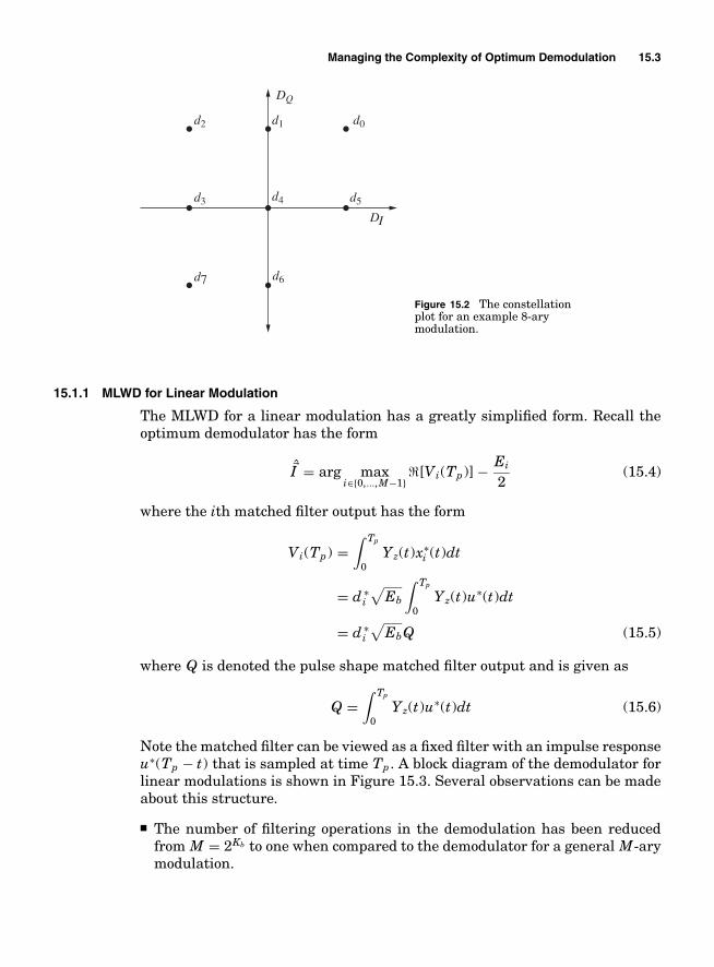
Managing the Complexity of Optimum Demodulation 15.3
DQ
DI
d0d1d2
d3 d4 d5
d6d7
Figure 15.2 The constellationplot for an example 8-arymodulation.
15.1.1 MLWD for Linear Modulation
The MLWD for a linear modulation has a greatly simplified form. Recall theoptimum demodulator has the form
�I = arg maxi∈{0,...,M−1}
[Vi(Tp)] − Ei
2(15.4)
where the ith matched filter output has the form
Vi(Tp) =∫ Tp
0Yz(t)x∗
i (t)dt
= d ∗i
√Eb
∫ Tp
0Yz(t)u∗(t)dt
= d ∗i
√EbQ (15.5)
where Q is denoted the pulse shape matched filter output and is given as
Q =∫ Tp
0Yz(t)u∗(t)dt (15.6)
Note the matched filter can be viewed as a fixed filter with an impulse responseu∗(Tp − t) that is sampled at time Tp. A block diagram of the demodulator forlinear modulations is shown in Figure 15.3. Several observations can be madeabout this structure.
■ The number of filtering operations in the demodulation has been reducedfrom M = 2Kb to one when compared to the demodulator for a general M-arymodulation.

15.4 Chapter Fifteen
Tp
DecisionDevice
QˆIYz(t) u∗ (Tp − t)
Figure 15.3 The block diagram of a demodulator for linear modulation.
■ The decision device can still potentially have a complexity that is O(2Kb).■ The energy of the ith transmitted signal is Ei = |di|2 Eb.
The optimum demodulator for linear modulation has an intuitively pleasinggeometric interpretation. The optimum demodulator can be expressed as
�I = arg maxi∈{0,...,M−1}
√Eb[d ∗
i Q] − |di|2 Eb
2(15.7)
Multiplying by 2 and adding a constant with respect to the possible transmittedsymbols, −|Q|2, gives
�I = arg maxi∈{0,...,M−1}
−|Q|2 + 2[d ∗i Q√
Eb] − |di|2 Eb
= arg maxi∈{0,...,M−1}
−∣∣Q − di
√Eb∣∣2
= arg mini∈{0,...,M−1}
∣∣Q − di
√Eb∣∣2 (15.8)
Consequently, the optimum demodulator computes Q and finds the possibletransmitted constellation point di
√Eb which has the minimum squared Eu-
clidean distance to Q. This is known by communications engineers as a mini-mum distance decoder. This minimum distance decoder induces decision regionsin the complex plane. These decision regions represent the matched filter out-put values that correspond to a most likely transmitted symbol. The decisionregions for 4PSK MLWD are shown in Figure 15.4. In the sequel the decisionregions will be denoted Ai where if Q ∈ Ai then I = i represents the MLWDoutput. It should be noted that the decision regions are bounded by the linesthat are defined as the equal distance points from each pair of constellationpoints. For instance, with QPSK there are four such lines and each decisionregion is bounded by two of these lines.
EXAMPLE 15.2Considering Example 15.1 the decision regions are defined as in Figure 15.5. The decisionregions here tend to have rectangular forms as the constellation is defined on a grid.The one notable exception is in the bottom right corner where there is a point missingfrom the grid.

Managing the Complexity of Optimum Demodulation 15.5
DQ
DI
A1
d1 Eb
d2 Eb
A2
A0
A3
d0 Eb
d3 EbFigure 15.4 The minimum dis-tance decision regions for 4PSK.
Recall the matched filter output when the ith word was transmitted has theform
Q =∫ Tp
0yz(t)u∗(t)dt =
∫ Tp
0xi(t)u∗(t)dt +
∫ Tp
0Wz(t)u∗(t)dt
= di
√Eb + Nz(Tp) (15.9)
With this view the signal portion of the matched filter output corresponds tothe transmitted symbol scaled by the bit energy,
√Eb, and the noise causes a
random translation of the signal in the complex plane. The idea of a minimum
DQ
DI
A0A1A2
A3 A4 A5
A6A7
Figure 15.5 The decision regions for the linear modulationgiven in Example 15.1.

15.6 Chapter Fifteen
QI
Q Nz(Tp)
Ebd0
Figure 15.6 An example geometric interpretation of the signaland noise in linear modulation. Dz = d0 =
√2e j π/4 = 1 + j .
distance decoder is simply trying to find which signal set would correspond tothe smallest noise magnitude. For example, if d0 from the 4PSK constellationin Figure 15.1 is the transmitted symbol then the matched filter output wouldhave a representation as given in Figure 15.6.
15.1.2 Error Rate Evaluation for Linear Modulation
The symbol error probability calculation also has a nice geometric interpreta-tion. Comparing the signal form in Figure 15.6 to decision regions in Figure 15.4an error will occur when the noise, Nz(Tp), pushes the matched filter outputinto a decision region that does not correspond to the transmitted symbol. SinceNz(Tp) is a complex Gaussian random variable with
var(Nz(Tp)) = Eu N0 = N0 var(N I (Tp)) = N0
2= var(N Q(Tp)) (15.10)
the PDF of the noise is easily computed using Eq. (10.26). An example noisePDF is plotted in Figure 15.7(a). The probability of word error conditioned onthe ith symbol being sent is
PW (E| �I = i) = P (Q �∈ Ai| �I = i) = P (di
√Eb + Nz(Tp) �∈ Ai) (15.11)
Consequently, this probability is simply an integral of the noise PDF, i.e.,
PW (E|i) =∫
Ri
f Nz(nz)d nz =∫
1Ri (nz) f Nz(nz)d nz (15.12)

Managing the Complexity of Optimum Demodulation 15.7
Figure 15.7 A noise PDF corresponding to var(Nz(Tp)) = 1 and the masking needed to compute the word errorrate for QPSK modulation.
where the indicator function is used to mask the PDF only in the regions wherenoise will cause an error. Figure 15.7(b) shows the masked PDF for a 4PSKdecision regions given in Figure 15.4 for d0 = √
2 exp( j π4 ).
EXAMPLE 15.3For the linear modulation presented in Example 15.1 several of the integration regionsfor conditional word error rates can be computed in close form. For example, the condi-tional word error rate for �I = 4 is given as
PW (E| �I = 4) = 1 −∫ b
−b
∫ b
−bf Nz(nz)d nz (15.13)
where b = A√
Eb2 . Likewise, the conditional error rate for �I = 1 is
PW (E| �I = 1) = 1 −∫ b
−b
∫ ∞
−bf Nz(nz)d nz (15.14)
The conditional decision region for �I = 5 is a bit more complex but it is still easilyspecified and the integration can be completed.
The PW (E) for a given Kb can be a significant function of how the con-stellation points are placed in the complex plane. For example, consider twocommon linear modulations, pulse amplitude modulation (PAM) and phaseshift keyed (PSK) modulation that have been implemented often in engineer-ing practice. PSK uses only the phase to transmit information while PAMuses only the amplitude to transmit information. Examples of the constella-tion plots for these two modulations are shown in Figure 15.8(a) for Kb = 2.
-4 -3 -2 -1 0 1 2 3 4
-4-2
0
240
0.05
0.1
0.15
0.2
x
y
f XY
(x, y
)
(a) Noise PDF
f XY
(x, y
)
(b) Noise PDF after masking,d0 = 1 + j, Eb = 1
0.10.080.060.040.02
04 3 2 1 0 -1 -2 -3 -4
-4-3-2-101234
y
x

15.8 Chapter Fifteen
DI
DQ
4 PSK
4 PAM
(a) Constellation plots (b) Word error rate curves
100
1086420 12 14 16
BPSK4-PAM4-PSK
10−1
10−2
10−3
10−4
10−5
10−6
PW
(E)
Eb/N0, dB
Figure 15.8 Constellation diagrams and word error rate curves comparing 4PAM and 4PSK.
Note 4-ary pulse amplitude modulation (4PAM) is characterized with �d ={±√
2/√
5, ±3√
2/√
5}. It is clear from the constellation plot that the points ofQPSK are farther apart than the points for 4PAM and hence QPSK will be ableto send 2 bits of information with more fidelity than 4PAM. The PW (E) for eachof these linear modulations are given for Kb = 1, 2 as (see problems)
PW (E) = 12
erfc
(√Eb
N0
)BPSK/BPAM (15.15)
PW (E) = erfc
(√Eb
N0
)−(
12
erfc
(√Eb
N0
))2
4PSK (15.16)
PW (E) = 34
erfc
⎛⎝√
2Eb
5N0
⎞⎠ 4PAM (15.17)
These curves are plotted in Figure 15.8(b). It is clear from Figure 15.8(b) thatthe manner in which constellation points are chosen in sending Kb bits with alinear modulation can have a significant impact on the error rate.
The union bound for the word error probability of a linear modulation isstraightforward to compute. The union bound can be formed by noting that thepairwise Euclidean squared distance is given as
�E (i, j ) = Eb|di − d j |2 (15.18)
Consequently, the union bound can be formed by looking only at the constella-tions. The union bound is not a function of the pulse shape used in the linearmodulation.

Managing the Complexity of Optimum Demodulation 15.9
EXAMPLE 15.4Considering Example 15.1 the complete union bound would have to consider sevendifferent distances for each postulated transmitted signal. Just like MPSK in Chapter 14this union bound can be tightened. For example, for �I = 0 the conditional unionbound is
PWUB(E| �I = 0) = 12
erfc
(√�E (1, 0)
4N0
)+ 1
2erfc
(√�E (5, 0)
4N0
)(15.19)
for �I = 1 the conditional union bound is
PWUB(E| �I = 1) = 12
erfc
(√�E (0, 1)
4N0
)+ 1
2erfc
(√�E (2, 1)
4N0
)+ 1
2erfc
(√�E (4, 1)
4N0
)
(15.20)for �I = 4 the conditional union bound is
PWUB(E| �I = 4) = 12
erfc
(√�E (1, 4)
4N0
)+ 1
2erfc
(√�E (3, 4)
4N0
)+ 1
2erfc
(√�E (5, 4)
4N0
)
+12
erfc
(√�E (6, 4)
4N0
)(15.21)
and for �I = 5 the conditional union bound is
PWUB(E| �I = 5) = 12
erfc
(√�E (0, 5)
4N0
)+ 1
2erfc
(√�E (4, 5)
4N0
)+ 1
2erfc
(√�E (6, 5)
4N0
)
(15.22)Combining all the conditional union bounds and noting that adjacent points have a
Euclidean distance of �E (1, 0) =√
12Eb5 and points separated on a diagonal have a
distance of �E (6, 5) =√
24Eb5 the union bound is given as
PWUB(E) = 54
erfc
(√3Eb
5N0
)+ 1
8erfc
(√6Eb
5N0
)(15.23)
So an additional benefit of linear modulation beside the simple MLWD is thatthe PW (E) can always be easily computed. The actual word error probabilitycalculation might require a little computer work (two dimensional numericalintegration) but this effort is not unreasonable for a modern communicationengineer. The full union bound is easily computed. Tighter union bounds areeasily identified by looking at the decision regions. While often a general M-arymodulation must resort to a full union bound computation to characterize thePW (E) this is not necessary for linear modulation.

15.10 Chapter Fifteen
15.1.3 Spectral Characteristics of Linear Modulation
For linear modulations the average energy spectrum per bit is straightforwardto compute. Using the definition of the energy spectrum per bit gives
Dxz(f ) = E[Gxz(f )]Kb
= Gu(f )EbE[|Dz|2]
Kb= Gu(f )
Eb∑M−1
i=0 |di|2πi
Kb= EbGu(f )
(15.24)
The important point to note about Eq. (15.24) is that the average energy spec-trum per bit is entirely (up to a constant multiple) a function of the pulse shapespectrum, Gu(f ). Transmitting more bits (increasing Kb) has no effect on theoccupied spectrum. Consequently, with a bandwidth efficient choice of the pulseshape, u(t), linear modulation is a very effective modulation for bandlimitedchannels. A design of a pulse shape that will meet a specified spectral mask isexplored in the projects at the end of Chapter 13.
15.1.4 Example: Square QuadratureAmplitude Modulation
This section will be concluded with a discussion of square quadrature amplitudemodulation (QAM) which is a commonly used linear modulation in engineeringpractice. A square QAM constellation consists of a square of M1 points by M1points with the M1 points in each dimension placed on a equally spaced grid.Normally the square is chosen such that M1 = 2Kb/2 so that an integer numberof bits is used to specify the constellation in each dimension. This constellationis considered in detail in the homework problems and the important results tohighlight here are that the spectral efficiency increases logarithmically withM1 and that the word error probability of this modulation is upperbounded as
PW (E) ≤ 1 −⎛⎝erf
⎛⎝√
6 log2(M1)M2
1 − 1Eb
N0
⎞⎠⎞⎠
2
(15.25)
A plot of this bound to the word error probability is given in Figure 15.9 forvarious M1. Much like was seen earlier in MPSK the word error performancesignificantly degrades for a fixed SNR as the spectral efficiency is increased. Tokeep the same level of performance the signal to noise ratio must be increasedby 4 dB as the spectral efficiency increases by 2 bits/s/Hz.
15.1.5 Summary of Linear Modulation
Important points about linear modulation are
■ Demodulation complexity of linear modulation does not increase exponen-tially with the number of bits transmitted since only one matched filter outputneeds to be computed and simple decision regions can be identified. Linearmodulation is often used because it has a low demodulation complexity.

Managing the Complexity of Optimum Demodulation 15.11
0 5 10 15 20
10−1
100
Wor
d E
rror
Pro
babi
lity
M1=1M1=2M1=3M1=4
10−2
10−3
10−4
10−5
10−6
Eb/N0, dB
Figure 15.9 The word error probability bound for square QAM.
■ The energy spectrum per bit of a linear modulation is entirely a function ofthe pulse shape that is used. Bandwidth efficient pulse shapes are often usedin conjunction with M-ary linear modulation when bandwidth efficiency is ofparamount importance. This will be examined in more detail in Chapter 16.
■ Fidelity in message reconstruction gets significantly worse as M gets larger.This can be seen by examining the error rate of linear modulations in bothFigure 15.8(b), Figure 15.9, and Figure 14.8. Consequently, linear modula-tion provides a classic trade-off in bandwidth efficiency (bandwidth efficiencyis proportional to Kb) versus fidelity (fidelity significantly degrades withincreasing Kb).
■ The selection of the constellation points in an M-ary linear modulation cansignificantly affect the resulting error rate. This can be seen by examin-ing the performance of 4PAM and 4PSK (both Kb = 2) in Figure 15.8(b).4PAM has a 3-dB worse performance than 4PSK since the 4PAM constel-lation points have not been placed as effectively in the complex plane asthe 4PSK constellation points. A more general demonstration of this point isshown in Figure 15.10 where the performance of the square QAM is comparedto Shannon’s bound and the other modulations introduced up until this point.Clearly a QAM modulation by placing constellation points more judiciouslyin the complex plane can provide better performance at a common spectral ef-ficiency than an MPSK modulation. The interesting characteristic of QAM is

15.12 Chapter Fifteen
0
2
4
6
8
10
−5 0 5 10 15 20
Upperbound
MPSK
MFSK
Square QAM
Spec
tral
Eff
icie
ncy,
bps
/Hz
Eb/N0 dB
Figure 15.10 A comparison of the spectral efficiencies of the modulations introduced.
that it performance seems to parallel Shannon’s upperbound as spectral effi-ciency increases while MPSK’s performance fall away from Shannon’s boundas spectral efficiency increases. An interesting paper that investigates opti-mal and suboptimal constellations is [FGL+84].
It is interesting to note that computer modems introduced in Chapter 12have migrated to linear modulation over time. The increase in transmissiondata rate is achieved by an increase in Baud rate1 and an increase in the sizeof the constellation of the linear modulation used in the modem. Examples inthis evolution are documented in Table 15.1. It should be noted that in earlymodems the data rate had the following characteristic
Wb = log2(M) × Baud rate (15.26)
TABLE 15.1 Evolution of Baud rates and constellationsizes in voiceband computer modems
Modem Standard Data Rate Baud Rate M
V.22 1,200 bps 600 Hz 4V.22bis 2,400 bps 600 Hz 16V.32 9,600 bps 2,400 Hz 32V.32bis 14,400 bps 2,400 Hz 128V.34 28,800 bps 3,200 Hz 896
1Baud rate will be discussed later in this chapter when we introduce the idea of streammodulations.

Managing the Complexity of Optimum Demodulation 15.13
As modem standards became more sophisticated (V.32 and subsequent gen-erations) redundancy was added to the signaling to improve performance. Anoverview of how this redundancy helps improve the fidelity of message recon-struction is the focus of Chapter 17.
15.2 Orthogonal Modulations
The goal at this point is to identify a constraint that can be put on signaldesigns such that optimum demodulation can be formulated with a complexityof O(Kb). This linear complexity can be achieved if each bit can be demodulatedin an independent fashion. There is a simple constraint on the ML metric thatwill enable optimal bit-by-bit decisions. This section will focus on the case ofequal priors (πi = 1/M) but extension to the case of unequal priors is alsopossible. When there are Kb bits sent then if the ML metric can be expressedin an additive form as
T i =Kb∑
k=1
T (k)mk
(15.27)
where { �I } = {I (1) = m1, · · · , I (Kb) = mKb} then each bit can be demodulatedin an independent fashion. In other words, if each T i can be broken up intoa sum of terms which are individually only a function of a single bit position,k, and bit value for that position, I (k) = mk then independent bit demodu-lation can be implemented. This sum form means that finding the maximumlikelihood is found by a series of binary maximizations on each term of thesummation, i.e.,
�I = [ I (1) . . . I (Kb)] = arg maxi∈{0,...,M−1}
T i =[
arg maxm1
T (1)(m1) . . . arg max
mKb
T (Kb)(mKb )
](15.28)
This bit-by-bit maximization has a complexity that is O(Kb) as opposed toO(2Kb) that is the general case.
Many of the modulation schemes that are used in practice for their reducedcomplexity optimal demodulation are due to the following property.
Property 15.1 (Orthogonal Modulations) If Kb bits are transmitted by summing upKb waveforms each used to transmit a single bit, i.e.,
xi(t) =Kb∑l=1
x(ml, l, t) (15.29)
where again �I = i = [m1 m2 . . . mKb] and x(ml, l, t) is the waveform used to transmitI (l) = ml then the ML metric can be put in the additive form required for simplified bitdetection if the waveforms used to transmit each of the bits are orthogonal, i.e.,
[∫ ∞
−∞x(ml, l, t)x∗(mk , k, t) dt
]= 0 ∀k �= l, ml = 0, 1, mk = 0, 1 (15.30)

15.14 Chapter Fifteen
Proof: The ML metric consists of two components: the matched filter outputand the energy correction term. The matched filter term for the transmittedsignal that has the form in Eq. (15.29) is given as
[∫ ∞
−∞yz(t)x∗
i (t)dt]
= [∫ ∞
−∞yz(t)
(Kb∑l=1
x(ml, l, t)
)∗
dt
]
=Kb∑l=1
[∫ ∞
−∞yz(t)x∗(ml, l, t)dt
](15.31)
Consequently, just due to the form in Eq. (15.29) the matched filter output hasthe additive form required for simplified detection. The remaining term is theenergy correction term given for Eq. (15.29) as
Ei
2= 1
2
∫ ∞
−∞|xi(t)|2dt = 1
2
∫ ∞
−∞
Kb∑l=1
x(ml, l, t)
(Kb∑
k=1
x(mk , k, t)
)∗
dt
= 12
Kb∑l=1
∫ ∞
−∞|x(ml, l, t)|2dt + 1
2
Kb∑l=1
Kb∑k=1k �=l
∫ ∞
−∞x(ml, l, t)(x(mk , k, t))∗ dt
(15.32)
= 12
Kb∑l=1
Ex(ml,l) +Kb∑l=2
l−1∑k=1
[∫ ∞
−∞x(ml, l, t)(x(mk , k, t))∗ dt
](15.33)
where Ex(ml, l) is the energy of x(ml, l, t), i.e.,
Ex(ml, l) =∫ Tp
0|x(ml, l, t)|2 dt (15.34)
Clearly the second term in Eq. (15.33) will go to zero if the orthogonality condi-tion holds and then the energy correction term will also have an additive form.Using these results it is apparent that
T (k)mk
= [∫ ∞
−∞yz(t)x∗(mk , k, t) dt
]− Ex(mk , k)
2� (15.35)
An interesting characteristic of orthogonal modulations is that the deci-sion metric has exactly the same form as the single bit detector presented inChapter 13. Using the above notation for orthogonal modulation we see thatthe optimal decision rule for each bit is now given as
exp
[2T (k)
1
N0
]π1
I (k)=1><
I (k)=0
exp
[2T (k)
0
N0
]π0 (15.36)

Managing the Complexity of Optimum Demodulation 15.15
The MLBD has the form
T (k)1
I (k)=1><
I (k)=0
T (k)0
[V1(k)] − 12
Ex(1,k)
I (k)=1><
I (k)=0
[V0(k)] − 12
Ex(0,k) (15.37)
where
Vmk (k) =∫ ∞
−∞Yz(t)x∗(mk , k, t) dt (15.38)
is the matched filter to the waveform used to transmit I (k) = mk . This struc-tural characteristic of orthogonal modulations implies that Kb bits can opti-mally be demodulated by Kb binary demodulators operated in parallel. Thesebinary demodulators have the same form as discussed in Chapter 13 and is thereason why so much effort was spent characterizing the single bit demodulator.Well over 95% of the communications systems in the world utilize orthogo-nality in some form so Chapters 13 and 14 are fundamental material in theunderstanding of digital communication. With orthogonal modulation optimaldemodulation now has a complexity of O(Kb) as desired in practical communi-cation systems.
While orthogonality seems to offer a solution to the complexity issue, theorthogonality exacts a price in the fidelity of demodulation. Since the orthog-onality reduces the demodulation to exactly that of a single bit developedin Chapter 13 we can deduce the performance is exactly that of the singlebit demodulator. Consequently, the bit error probability performance is lowerbounded by
PB (E, k) = 12
erfc
⎛⎝√
�E (1, 0, k)4N0
⎞⎠ ≥ 1
2erfc
(√Eb
N0
)(15.39)
where �E (1, 0, k) is the Euclidean square distance between the two waveformsused to send the kth bit, i.e.,
�E (1, 0, k) =∫ ∞
−∞|x(1, k, t) − x(0, k, t)|2 dt (15.40)
The orthogonality implies each decision is independent. This independence im-plies that the word error probability for an orthogonal modulation when each bitis sent with waveforms that have the same Euclidean square distance becomes

15.16 Chapter Fifteen
(see Problem 15.12)
PW (E) = 1 −Kb∏
k=1
(1 − PB (E, k))
= 1 − (1 − PB (E))Kb ≥ 1 −(
1 − 12
erfc
(√Eb
N0
))Kb
(15.41)
The unfortunate consequence of orthogonality is that the performance of singlebit demodulation is far from Shannon’s bound as detailed in Chapter 13.
Orthogonal modulations offer an interesting trade-off for digital communica-tion system designers. Orthogonality allows the complexity of optimal demodu-lation to be O(Kb) as would be desired when Kb is large. For this reason almostall communication systems in practice use orthogonality in some form. Ortho-gonality with independent bit modulation waveforms limits the achievableperformance to be far from Shannon’s bound and is not desirable in moderncommunication systems. In practice orthogonality is still used because thereare techniques that can be used in conjunction with orthogonal modulations tomove performance close to Shannon’s bound. These techniques will be brieflyoverviewed in Chapter 17
15.3 Orthogonal Modulation Examples
15.3.1 Orthogonal Frequency Division Multiplexing
A commonly used modulation that admits a simple optimal bit demodulation isorthogonal frequency division multiplexing (OFDM) [Cha66]. OFDM has foundutility in telephone, cable, and wireless modems. With OFDM each of the Kbbits is independently modulated on a separate subcarrier frequency and thesubcarrier frequencies are chosen to ensure the orthogonality. The format foran OFDM signal is
Xz(t) =
⎧⎪⎪⎨⎪⎪⎩
Kb∑l=1
Dz(l)
√Eb
Tpexp[ j 2π fd (2l − Kb − 1)t] 0 ≤ t ≤ Tp
0 elsewhere
(15.42)
where Dz(l) = a(I (l)) and 2 fd is the separation between adjacent frequenciesthat are used to transmit the information. The transmission rate of this formof OFDM is Wb = Kb/Tp bits/s. In examining Eq. (15.42) it is clear that in thisform of OFDM a binary linear modulation is used on each of the Kb differentsubcarrier frequencies. For clarity of discussion the remainder of the sectionwill assume the linear modulation is BPSK (i.e., a(0) = 1 and a(1) = −1). Amore general form of OFDM could use any type of linear modulation and anynumber of bits per subcarrier. For example, 4 bits could be transmitted perfrequency using a 16QAM modulation (see Section 15.1.4 and Problem 15.1).Some of the generalizations of OFDM will be explored in the homework.

Managing the Complexity of Optimum Demodulation 15.17
−15 −10 −5 0 5 10 15 20−15
−10
−5
0
5
10
15
x Q(t
)
xI(t)
(b) Kb = 64
−2 −1.5 −1 −0.5 0 0.5 1 1.5 2−2
−1.8
−1.6
−1.4
−1.2
−1
−0.8
−0.6
−0.4
−0.2
0
xI(t)
x Q(t
)
(a) Kb = 4, I = [0 0 1 0].
Figure 15.11 Example vector diagrams of OFDM transmissions.
The OFDM transmitted waveform is a sum of Kb complex sinusoids. Thistransmitted waveform will have a complex envelope that changes significantlyover the transmission time as the Kb complex sinusoids change in phase relativeto each other. The larger the value of Kb the larger this variation over the trans-mission time will be. Figure 15.11 shows the vector diagrams of some exampleOFDM transmitted waveforms. The vector diagram clearly becomes more com-plex as more bits are transmitted. In addition, the peak value of the amplitudeof the complex envelope increases with Kb. For example, Figure 15.12 showsxA(t) of some example OFDM transmitted waveforms. An OFDM waveform has
0 0.2 0.4 0.6 0.8 10.8
1
1.2
1.4
1.6
1.8
2
2.2
2.4
2.6
2.8
x A(t
)
Normalized Time, t/Tp
0 0.2 0.4 0.6 0.8 102
4
6
8
10
12
14
16
18
x A(t
)
Normalized Time, t/Tp
(b) Kb = 64(a) Kb = 4, I = [0 0 1 0].
Figure 15.12 Example xA(t) for OFDM transmissions.

15.18 Chapter Fifteen
a significant difference between the peaks in amplitude and the average valueof the amplitude. This high peak to average ratio (PAPR)2 requires the radios inan OFDM system to have a large dynamic range to process the signal withoutdistortion.
In the general framework of orthogonal modulations OFDM has set
x(ml, l, t) =
⎧⎪⎪⎪⎨⎪⎪⎪⎩
dml
√Eb
Tpexp[ j 2π fd (2l − Kb − 1)t] 0 ≤ t ≤ Tp
0 elsewhere
(15.43)
The orthogonality condition then corresponds to
[∫ ∞
−∞x(ml, l, t)x∗(mk , k, t)dt
]= 0 (15.44)
[dml d
∗mk
Eb
Tp
∫ Tp
0exp[ j 4π fd (l − k)t]dt
]= 0 (15.45)
Using the result of Eq. (13.86) shows that the minimum spacing with an arbi-trary complex constellation for orthogonality is achieved with fd = 1/(2Tp). Ifthe constellation is restricted to have real values (e.g., BPSK) then the mini-mum frequency spacing is achieved with fd = 1/(4Tp).
EXAMPLE 15.5The wireless local area network standard denoted IEEE 802.11a uses OFDM. The802.11a standard uses OFDM that can be represented with Kb = 53 with Tp = 3.2 µs.The frequency spacing of the subcarrier tones is set with fd = 156.25 kHz becausecomplex constellations are used in some modes of transmission. The potential trans-mission rate of the 802.11a waveform with BPSK modulation would be 16.25 MHz. Thetop transmission speed of 54 Mbps is achieved by using a QAM modulation on eachsubcarrier. QAM constellations are investigated Section 15.1.4 and in the problems atthe end of the chapter.
The optimal demodulator has the form of Kb parallel single bit optimal de-modulators. This demodulator is shown in Figure 15.13. Restricting ourselvesto BPSK modulation on each subcarrier frequency the MLBD has the form
[∫ Tp
0Yz(t)
√1
Tpexp[− j 2π fd (2k − Kb − 1)t]dt
]= [Q(k)]
I (k)=0><
I (k)=1
0 (15.46)
2See the definition of PAPR in Chapter 5.

Managing the Complexity of Optimum Demodulation 15.19
••••
ThresholdTest
0
0
I(Kb)
Yz(t)
1Tp
Tp∫0Yz(t)exp[−j2π f1t]dt
1Tp
Tp∫0Yz(t)exp[−j2π fkb
t]dt
Re[•] I(1)ˆ
ˆRe[•]
ThresholdTest
Figure 15.13 The optimal demodulator for OFDM using BPSK.
Since OFDM is using a linear modulation on each subcarrier we will use Q(k) todenote the matched filter output for the kth bit or subcarrier. The demodulatorcomputes a filter output for each bit, k ∈ {1, . . . , Kb}, and hence the complexityof the OFDM optimum demodulator is O(Kb) as opposed to the O(2Kb) for anarbitrary modulation that transmits Kb bits of information. For future refer-ence here we note that Q(k) can be viewed at the Fourier transform of Yz(t)evaluated at f = f k = fd ((2k − Kb − 1). The optimal OFDM demodulatorevaluates the real part of the Fourier transform at Kb points symmetricallyspaced around f = 0 and uses these Fourier transform values in a thresholdtest. Since [Q(k)] = Dz(k)
√Eb + N I (k) where var(N I (k)) = N0
2 , the bit errorprobability performance of OFDM using BPSK on each subcarrier is clearly
PB (E) = 12
erfc
(√Eb
N0
)(15.47)
The optimal demodulator for OFDM is essentially Kb single bit demodulatorsimplemented in parallel (one for each subcarrier). Because of the orthogonalityof the subcarriers the fidelity achieved by an OFDM demodulator is the sameas the demodulator for a single bit transmitted in isolation (see Chapter 13).
Spectral Characteristics of OFDM
Recall that the average energy spectrum per bit is
Dxz(f ) = E[Gxz(f )]Kb
(15.48)
To simplify the notation needed in this discussion we will make the followingdefinition.

15.20 Chapter Fifteen
Definition 15.1 The Fourier transform of the unit energy rectangular pulse function
ur (t) =
⎧⎨⎩
1√Tp
0 ≤ t ≤ Tp
0 elsewhere
(15.49)
is
Ur (f ) =√
Tpsin(π f Tp)
π f Tpexp[− j π f Tp] (15.50)
Taking the Fourier transform of the OFDM signal in Eq. (15.42) and using thefrequency shift property of the Fourier transform gives
Xz(f ) =Kb∑l=1
Dz(l)√
EbUr ( f − fd (2l − Kb − 1)) (15.51)
The energy spectrum is then given as
GXz(f ) = Eb
Kb∑l1=1
Kb∑l2=1
Dz(l1)D∗z (l2)Ur ( f − fd (2l1−Kb−1))U ∗
r ( f − fd (2l2−Kb−1))
(15.52)The average energy spectrum per bit is then
DXz(f ) = Eb
KbE
⎡⎣ Kb∑
l1=1
Kb∑l2=1
Dz(l1)D∗z (l2)
×Ur ( f − fd (2l1 − Kb − 1))U ∗r ( f − fd (2l2 − Kb − 1))
⎤⎦ (15.53)
The average energy spectrum per bit can be greatly simplified when BPSKmodulation is used on each frequency in OFDM. Recall each bit is assumed tobe random and independently distributed. Here it will be further assumed thatthe bits are identically distributed with P (I (k) = 0) = π0 and P (I (k) = 1) = π1for k = 1, . . . , Kb. Examining the term corresponding to a fixed l1 and l2, l1 �= l2,in Eq. (15.53) (one of K2
b terms in the summation) gives
E[Dz(l1)D∗z (l2)]Ur ( f − fd (2l1 − Kb − 1))U ∗
r ( f − fd (2l2 − Kb − 1))
= (π0π0 + π1π1 − π0π1 − π1π0)Ur ( f − fd (2l1 − Kb − 1))
×U ∗r ( f − fd (2l2 − Kb − 1)) = (π0 − π1)2
×Ur ( f − fd (2l1 − Kb − 1))U ∗r ( f − fd (2l2 − Kb − 1)) (15.54)
Examining the term corresponding to l1 = l2, in Eq. (15.53) gives
E[|Dz(l1)|2]|Ur ( f − fd (2l1 − Kb − 1))|2
= (π0 + π1)|Ur ( f − fd (2l1 − Kb − 1))|2
= |Ur ( f − fd (2l1 − Kb − 1))|2 (15.55)

Managing the Complexity of Optimum Demodulation 15.21
The average energy spectrum per bit is then given as
DXz(f ) = Eb
Kb
Kb∑l1=1
|Ur ( f − fd (2l1 − Kb − 1))|2 + Eb
Kb(π1 − π0)2
(15.56)
×Kb∑
l2=1
Kb∑l1=1l1 �=l2
Ur ( f − fd (2l1 − Kb − 1))U ∗r ( f − fd (2l2 − Kb − 1))
Further simplifications occur if each bit is equally likely. For equally likelybits the second term in Eq. (15.56) becomes zero. The spectrum in this casebecomes
DXz(f ) = Eb
Kb
Kb∑l=1
|Ur ( f − fd (2l − Kb − 1))|2 (15.57)
This spectrum is plotted in Figure 15.14 (the solid line) for Kb = 4 and fd =0.5/Tp. The dashed lines in Figure 15.14 represent the energy spectrum ofeach modulated subcarrier of the OFDM waveform. The conclusions we can
−6 −4 −2 0 2 4 6−50
−45
−40
−35
−30
−25
−20
−15
−10
−5
0
Dx z
(f)/
Eb,
dB
Normalized Frequency, f Tp
Figure 15.14 Average energy spectrum per bit for OFDM. Kb = 4, equally likely bits andBPSK modulation, with fd = 1/(2Tp).

15.22 Chapter Fifteen
draw about the average energy spectrum of OFDM is that the bandwidth oc-cupancy for this type of an OFDM is proportional to 1/Tp and to Kb. Recallthat the transmission rate is Wb = Kb/Tp bits/s. Consequently, the transmis-sion spectral efficiency is in the neighborhood of 1 bit/s/Hz, though the exactnumber will be a function of how the engineering bandwidth is defined.
In conclusion OFDM provides a method to implement multiple bit transmis-sion with good performance and reasonable complexity and spectral efficiency.The bit error probability performance of the OFDM scheme highlighted in thissection gives the same bit error probability performance as BPSK used in isola-tion. The spectral efficiency is roughly 1 bit/s/Hz. The complexity of the optimumreceiver is O(Kb). Consequently, OFDM has found significant utility in engi-neering practice. One issue with OFDM is that the signal has a large PAPRand this characteristic can require a high performance and costly radio systemto get high fidelity in message reconstruction.
15.3.2 Orthogonal Code Division Multiplexing
A second commonly used modulation that admits a simple optimal bit de-modulation is orthogonal code division multiplexing (OCDM). OCDM is oftenused in cellular radio communication and in satellite communication on thedownlink. For OCDM, each of the Kb bits is independently modulated on thesame carrier frequency with an orthogonal waveform. This orthogonal wave-form is often termed the spreading waveform. The typical format for an OCDMsignal is
Xz(t) =
⎧⎪⎨⎪⎩
Kb∑l=1
Dz(l)√
Ebsl(t) 0 ≤ t ≤ Tp
0 elsewhere
(15.58)
where D(l) = a(I (l)) and sl(t) is often denoted the spreading signal for the lthbit. Here we assume that both E[|D(l)|2] = 1 and that Esl = 1. The transmissionrate of this form of OCDM is Wb = Kb/Tp bits/s. In examining Eq. (15.58)it is clear that in this form of OCDM a binary linear modulation is used oneach of the Kb different spreading waveforms. Again for clarity of discussionthe remainder of the section will assume the linear modulation is BPSK (i.e.,a(0) = 1 and a(1) = −1). It should be noted that OFDM is a special case ofOCDM with sl(t) = exp[ j 2π f lt]/
√Tp.
In the general framework of orthogonal modulations OCDM has set
x(ml, l, t) ={
dml
√Ebsl(t) 0 ≤ t ≤ Tp
0 elsewhere(15.59)
The orthogonality condition then corresponds to
[∫ ∞
−∞x(ml, l, t)x∗(mk , k, t)dt
]= Eb
[dml d
∗mk
∫ Tp
0sl(t)s∗
k(t) dt]
= 0 (15.60)

Managing the Complexity of Optimum Demodulation 15.23
Tp
Tp
1Tp
s1(t)
s2(t)1Tp
1Tp
−
s4(t)
s3(t)
Tp
Tp
Figure 15.15 Example spreading waveforms for OCDM and Kb = 4.
The remaining question is how to find a set of Kb orthogonal waveforms. Thereis a wide variety of ways to construct these waveforms and one example is givenin Figure 15.15 for Kb = 4. Certainly this construction is not unique. The timewaveform of OCDM can have significant variations across the transmissiontime. For instance Figure 15.16 shows the time plot of the output envelope3 oftwo possible transmitted waveforms for the spreading waveforms introduced inFigure 15.15 for Kb = 4. In both cases the transmitted energy is equal but howthat energy is spread across the transmit time is very much a function of thetransmitted information. An OCDM waveform has a large PAPR. The PAPRwill increase as Kb increases. This high PAPR requires the radios in an OCDMsystem to have a large dynamic range to process the signal without distortion.
EXAMPLE 15.6One of the standards for mobile telephones is denoted IS-95. IS-95 is primarily a voicecommunication system and voice communications can be achieved with transmissionrates of less than 10 kHz with modern voiceband source encoders. IS-95 uses OCDM asthe forward link modulation with Kb = 64. The spreading waveforms used to send eachbit are Walsh functions which are discussed in Problem 15.22 (This problem shows howWalsh functions are derived from Hadamard matrices). In IS-95 Tp = 52.083 µs so ifBPSK modulation was used a bit rate of 1.2288 Mbps could be achieved. In voice mobiletelephony data rates only need to support voiceband speech transmission. Hence IS-95uses each of the spreading waveforms to transmit a bit to potentially 64 different users.This use of one physical layer radio link to support many information transactions isknown as multiple access communications. Each spreading waveform is simultaneouslycapable of supporting a 19.2 kbps transmission rate for each user which is a data rategreater than necessary for modern speech encoders.
3Because the spreading waveforms are all real xA(t) = |xI (t)|.

15.24 Chapter Fifteen
0 0.2 0.4 0.6 0.8 1−0.5
0
0.5
1
1.5
2
2.5
3
3.5
4
4.5
5
I = i1I = i2
x A(t
)
Normalized Time, t/Tp
Figure 15.16 Output envelope time waveforms for the spreading waveforms in Figure 15.15.i1 = [0 1 0 0] and i2 = [0 0 0 0].
The optimal demodulator again has the form of Kb parallel single bit optimaldemodulators. This demodulator is shown in Figure 15.17. Restricting ourselvesto BPSK modulation on each spreading waveform the MLBD has the form
[∫ Tp
0Yz(t)s∗
k(t) dt]
= [Q(k)]I (k)=0
><
I (k)=1
0 (15.61)
The demodulator computes a filter output for each bit, k ∈ {1, . . . , Kb}, and hencethe complexity of optimal OCDM demodulation is again O(Kb) as opposed toO(2Kb) for an arbitrary modulation that transmits Kb bits of information. Since[Q(k)] = Dz(k)
√Eb + N I (k) where var(N I (k)) = N0
2 , the bit error probabilityperformance of OCDM using BPSK on each spreading waveform is again
PB (E) = 12
erfc
(√Eb
N0
)(15.62)
The optimal demodulator for OCDM is again Kb single bit demodulators imple-mented in parallel (one for each orthogonal spreading waveform). Because ofthe orthogonality of the spreading waveforms the fidelity achieved by an OCDM

Managing the Complexity of Optimum Demodulation 15.25
…
ThresholdTest
ThresholdTest
0
0
Re •[ ] I(1)
I(Kb)
Yz(t)
TpYz(t)s1
* (t)dt
Tp∫0 Yz(t)s*Kb
(t)dt Re[•]
∫0
Figure 15.17 The optimal demodulator for OCDM using BPSK.
demodulator is the same as the demodulator for a single bit transmitted in iso-lation (see Chapter 13).
Spectral Characteristics of OCDM
Again the average energy spectrum per bit is
Dxz(f ) = E[Gxz(f )]Kb
= Eb
KbE
[Kb∑l=1
Kb∑k=1
Dz(l)D∗z (k)Sl(f )S∗
k(f )
](15.63)
Using the results of Section 15.3.1 and assuming for simplicity that each bit isequally likely and BPSK modulation is used, the spectrum in this case becomes
DXz(f ) = Eb
Kb
Kb∑l=1
|Sl(f )|2 (15.64)
where Sl(f ) = F{sl(t)}. The important thing to note here is that the spectrumof OCDM waveforms is directly proportional to the spectrum of the chosenspreading waveforms. The spectrum of the set of spreading signals chosen inFigure 15.15 (the solid line) is shown in Figure 15.18. The dashed lines inFigure 15.18 represent the energy spectrum of each modulated spreading signalof the OFDM waveform. The conclusions we can draw about the average energyspectrum of OCDM is that the bandwidth occupancy for this type of an OCDMis proportional to 1/Tp and to Kb. The bandwidth is greater than if a single bitwas sent in isolation since Kb orthogonal waveforms need to be constructed foreach of the Kb transmitted bits.
In conclusion OCDM provides a method to implement multiple bit transmis-sion with good performance and reasonable complexity and spectral efficiency.The bit error probability performance of the OCDM scheme highlighted in thissection gives the same bit error probability performance as BPSK used in isola-tion. The spectral efficiency is roughly 1 bit/s/Hz. The complexity of the optimum

15.26 Chapter Fifteen
−8 −6 −4 −2 0 2 4 6 8−50
−40
−30
−20
−10
0
10
Normalized Frequency, f Tp
Dx z
(f)/
Eb,
dB
Figure 15.18 The average energy spectrum per bit for the Kb = 4 example OCDM inFigure 15.15.
receiver is O(Kb). OCDM is a generalization of OFDM. Consequently, OCDMhas found significant utility in engineering practice. One issue with OCDM isthat the signal has a large PAPR and this characteristic can require a high per-formance and costly radio system to get high fidelity in message reconstruction.
15.3.3 Binary Stream Modulation
A third commonly used modulation that admits a simple optimal bit demodula-tion is orthogonal time division multiplexing. This is perhaps the most intuitiveform of orthogonal modulation. Orthogonal time division multiplexing is usedin a vast majority of digital communication systems in some form. The idea issimple, data is streamed in time (1 bit following another) and for the remain-der of this text this orthogonal time division multiplexing will be referred to asstream modulation. With a stream modulation each of the Kb bits is indepen-dently modulated on the same carrier frequency with a time shifted waveform.The typical format for a stream modulation using linear modulation is
Xz(t) =Kb∑l=1
Dz(l)√
Ebu(t − (l − 1)T ) (15.65)

Managing the Complexity of Optimum Demodulation 15.27
where D(l) = a(I (l)), T is known as the symbol4 or bit time in stream modu-lations, and u(t) is the unit energy pulse of length Tu. The transmission rateof stream modulation is Wb = Kb/Tp bits/s. It should be noted that Tp =(Kb − 1)T + Tu and for large Kb that Wb ≈ 1/T .
Definition 15.2 The Baud rate of a stream modulation is WBau = 1/T .
The time shifted pulses are repeated every T seconds. Hence the rate at whichbits (or more generally multiple bit symbols) are put into the channel is theBaud rate. In examining Eq. (15.65) it is clear that in this stream modulationa binary linear modulation is used in each of the Kb different time intervals.Again for clarity of discussion the remainder of the section will assume thelinear modulation is BPSK (i.e., a(0) = 1 and a(1) = −1).
In the general framework of orthogonal modulations stream modulation hasset
x(ml, l, t) ={
dml
√Ebu(t − (l − 1)T ) 0 ≤ t ≤ Tp
0 elsewhere(15.66)
where again u(t) is denoted the pulse shape. The orthogonality condition thencorresponds to
0 = [∫ ∞
−∞x(ml, l, t)x∗(mk , k, t)dt
]
= Eb[dml d
∗mk
∫ ∞
−∞u(t − (l − 1)T )u∗(t − (k − 1)T )dt
]= Eb[dml d
∗mk
Vu((k − l)T )] (15.67)
where Vu(τ ) is the pulse shape correlation function defined in Chapter 2 as
Vu(τ ) =∫ ∞
−∞u(t)u∗(t − τ )dt. (15.68)
This orthogonal time shift condition is often known as Nyquist’s criterion forzero intersymbol interference (ISI) [Nyq28a]. The remaining question is howto design orthogonal time shifted waveforms. There is a wide variety of waysto construct these waveforms but the simplest way is to limit u(t) to only havesupport on [0, T ]. For example, if Kb = 4 one can choose T = Tp/4 and havethe set of time shifted waveforms as given in Figure 15.19. Certainly this con-struction is not unique. It is interesting to note with the waveforms chosenin Figure 15.19 the amplitude of the transmitted signal will be constant. Theability to more carefully control peak to average power ratio is one advantageof stream modulation.
4A generalization not considered in this chapter but frequently used in practice is the idea of asending multiple bit symbol (instead of a 1 bit symbol considered here) every T seconds in a streammodulation. Essentially this is a combination of linear modulation and stream modulation.

15.28 Chapter Fifteen
Tp
s1(t) = u(t)
s2(t) = u(t − T)
s3(t) = u(t − 2T)
s4(t) = u(t − 3T)
Tp
Tp
Tp
Figure 15.19 An example of time shifted pulses for a linear stream modulation and Kb = 4.
The optimal demodulator again has the form of Kb parallel single bit optimaldemodulators. Since the sample modulation format is repeated in time therequired filtering operation can be implemented with one filter sampled seriallyin time. This demodulator is shown in Figure 15.20. Restricting ourselves toBPSK modulation on each time shifted pulse the optimum demodulator hasthe form
[∫ Tp
0Yz(t)u∗(t − (k − 1)T )dt
]= [Q(k)]
I (k)=0><
I (k)=1
0 (15.69)
The demodulator has one filter output whose output is sampled for each bit,k ∈ {1, . . . , Kb}, and hence the complexity of the stream modulation optimumdemodulator is again O(Kb) as opposed to the O(2Kb). The pulse shape matchedfilter output will be referenced frequently in the sequel hence we formallydefine it.
Definition 15.3 Recall the pulse shape matched filter has an impulse response ho(t) =u∗(Tu − t), so that the pulse shape matched filter output is
Qu(t) =∫ Tp
0Yz(λ)u∗(λ + Tu − t)dλ (15.70)
where Tu is the pulse shape time support.
ThresholdTest
0
Sampler I (k)Yz(t) u*(Tu − t)
Tu + (k − 1)T
Re[•]
Figure 15.20 The optimal demodulator for stream modulations using BPSK.

Managing the Complexity of Optimum Demodulation 15.29
Using this definition it is easy to see that
Q(k) = Qu(Tu + (k − 1)T ) (15.71)
A characteristic of linear stream modulation that makes for an efficient modemimplementation is that only one filter is needed to implement the demodulator.This advantage of stream modulation over other orthogonal modulations ismuch more significant when the filter is implemented with analog circuits.This pulse shape matched filter only needs to be sampled at different times toobtain the sufficient statistics for demodulation. When filters are implementedwith digital cirucits the computational complexity required for demodulationof all orthogonal modulations is about the same. This is the reason that streammodulations dominated digital modem implementations up untill the 1980’s asmost processing was done with analog circuitry. As Moore’s Law kicked in andimplementations became predominantly digital other modulations like OFDMand OCDM became practical.
Finally, again the performance of stream modulation is upperbounded by theperformance of binary modulations transmitted in isolation. This is true since[Q(k)] = Dz(k)
√Eb + N I (k) where var(N I (k)) = N0
2 , the bit error probabilityperformance of stream modulation using BPSK is
PB (E) = 12
erfc
(√Eb
N0
)(15.72)
Spectral Characteristics of Stream Modulations
Again the average energy spectrum per bit is
Dxz(f ) = E[Gxz(f )]Kb
= Eb
KbE
[Kb∑l=1
Kb∑k=1
Dz(l)D∗z (k)U (f )U ∗(f ) exp[− j 2π f (l − k)T ]
]
(15.73)
Using the results of Section 15.3.1 and assuming for simplicity that each bit isequally likely and BPSK modulation is used, the spectrum in this case becomes
DXz(f ) = Eb
Kb
Kb∑l=1
|U (f )|2 = EbGu(f ) (15.74)
where U (f ) = F{u(t)} and Gu(f ) = |U (f )|2. The important thing to note hereis that the spectrum of linear stream modulation is directly proportional tothe spectrum of the chosen pulse shape. The spectrum of the linear streammodulation defined in Figure 15.19 is shown in Figure 15.21. The conclusionswe can draw about the average energy spectrum of stream modulation is thatthe bandwidth occupancy is also proportional to 1/Tp and to Kb.

15.30 Chapter Fifteen
−10 −8 −6 −4 −2 0 2 4 6 8 10−50
−45
−40
−35
−30
−25
−20
−15
−10
−5
0
Dx z
(f)/
Eb,
dB
Normalized Frequency, fTp
Figure 15.21 The average energy spectrum per bit for stream modulation for the example pulseshape given in Figure 15.19.
15.4 Conclusions
This chapter looked at two signal design techniques that simplify the optimaldemodulator structures: linear modulation and orthogonal modulation. Linearmodulation simplifies the demodulator by only requiring one matched filter.Linear modulation provides reduced performance but no bandwidth expansionas Kb grows larger. Consequently, linear modulations often find utility whenspectral efficiency is at a premium and the expected SNR is high. Orthogonalmodulation is a technique where Kb bits are transmitted by using orthogo-nal waveforms for each bit. The orthogonality of the individual bit waveformsenables each bit to be detected optimally with a complexity identical to thesituation where the bit was transmitted in isolation. Examples of orthogo-nal modulation included in this chapter were modulations where orthogonalitywas obtained by frequency spacing (OFDM), obtained by complex waveforms(OCDM), and obtained by time spacing (stream modulation). Both linear mod-ulation and orthogonal modulation provide optimal demodulation complexitythat scales better with Kb than does general signaling. Using signals designedas either a linear or an orthogonal modulation produces a fidelity upperbounded

Managing the Complexity of Optimum Demodulation 15.31
by the error rate of BPSK. Linear modulation is advantageous as it allows forspectral efficiencies greater than 1 bit/s/Hz and is typically why it is used inpractice. As a final note all deployed communication systems use stream modu-lation in some form even when using OFDM or OCDM. It is also estimated thatgreater than 90% of the digital communication systems use linear modulationsin some form.
15.5 Homework Problems
Problem 15.1. 16 quadrature amplitude modulation (QAM) is a linear modulationwith Di = DI i + j DQi where DI i, DQi ∈ {−3A, −A, A, 3A} that can be used totransmit 4 bits per symbol (Kb = 4).
(a) Find the value of A such that Eb is the average energy per bit.
(b) Find the decision regions corresponding to the values of Q for MLWD of16QAM.
(c) Is 16QAM a geometrically uniform signal set?
(d) Compute the probability of word error for MLWD, PW (E), for 16QAM andplot for Eb/N0 = 0, 15 dB.
(e) Compute the full union bound to the probability of word error for MLWD for16QAM and plot for Eb/N0 = 0, 15 dB. Hint: The union bound requires thecomputation of 15 distances for each of the 16 possible transmitted signalsso it might be useful to use the computer.
(f) It is possible to eliminate some terms in the union bound for 16QAM as wasdone for MPSK. Identify the union bound having the smallest number ofterms for 16QAM.
(g) Using the union bound result and assuming a pulse shape is chosen suchthat BT = 1/Tp plot the 16QAM spectral efficiency in Figure 14.9.
Problem 15.2. Consider the two 8-ary (Kb = 3) linear modulations whose constel-lations are given in Figure 15.22. One of the 8-ary constellations has four pointseach placed on two concentric circles. The other 8-ary constellation has eightpoints selected from the 16QAM (see Problem 15.1) constellation in a checker-board fashion.
a) Determine the value of each constellation point such that Eb is the energyper bit and �1 = �2.
b) Find the decision regions corresponding to the values of Q for MLWD ofthese two 8-ary modulations.
c) Which constellation has a better performance? Why? How does the perfor-mance of the best constellation compare to the 8-ary linear modulation in-troduced in Example 15.1?

15.32 Chapter Fifteen
DI
DQ
∆1
∆2
(a)
DIi
DQi
(b)
Figure 15.22 Two 8-ary constellation plots for linear modulations.
Problem 15.3. This problem examines the probability of word error for MLWD ofsome common linear modulations.
(a) Show that the probability of word error for 4PSK is given as
PW (E) = erfc
(√Eb
N0
)−(
12
erfc
(√Eb
N0
))2
(15.75)
(b) 4-ary equally spaced pulse amplitude modulation (PAM) has a constellationthat is characterized with �d = {±√2/5, ±3
√2/5}. Show that the proba-
bility of word error for 4PAM is given as
PW (E) = 34
erfc
⎛⎝√
2Eb
5N0
⎞⎠ (15.76)
(c) Plot the spectral efficiency versus Eb/N0 of 4PAM on Figure 14.9 using aword error rate of 10−5.
Problem 15.4. This problem examines the union bound to the probability of worderror for MLWD of some common linear modulations.
(a) Show that the full union bound for the word error probability of 4PSK isgiven as
PW (E) = erfc
(√Eb
N0
)+ 1
2erfc
⎛⎝√
2Eb
N0
⎞⎠ (15.77)

Managing the Complexity of Optimum Demodulation 15.33
(b) There is a way to tighten the union bound for 4PSK, give the tightest unionbound to the word error probability.
(c) Show that the full union bound for the word error probability of 4PAM(�d = {±√2/5, ±3
√2/5}) is given as
PW (E) = 34
erfc
⎛⎝√
2Eb
5N0
⎞⎠+ 1
2erfc
⎛⎝√
8Eb
5N0
⎞⎠+ 1
4erfc
⎛⎝√
18Eb
5N0
⎞⎠(15.78)
(d) There is a way to tighten the union bound for 4PAM, give the tightest unionbound to the word error probability
Show that these results are tight to the true values given in Problem 15.3 athigh SNR.
Problem 15.5. Imagine that digital computers were first developed with five logiclevels to match the number of fingers on the typical human hand. Digitalcommunications would have evolved to be the transmission of quinits (havingfive possible values) as opposed to the transmission of bits. In this problem youwill consider what this course might have been like if this alternate evolutionhad occurred.
Consider a 5-ary modulation of the form Xz(t) = Dzu(t) corrupted by an addi-tive white Gaussian noise with one-sided spectral density of N0. Consider twopossible signal sets:
i d (1)i d (2)
i
0 1 A1 exp
( j 2π
5
)j A
2 exp( j 4π
5
) −A
3 exp( j 6π
5
) − j A
4 exp( j 8π
5
)0
where A is a positive real constant.
(a) Choose the value of A such that both signal sets have the same average Es.
(b) Give the demodulator that minimizes the word error probability and definethe decision regions for each of the two possible signal sets.
(c) Is either signal set geometrically uniform?
(d) Compute the full union bound to PW (E) for each of the two signal sets.
(e) Simplify the union bound as much as possible for each signal set by elimi-nating terms from the full union bound if possible.
(f) Use numerical integration to compute the actual PW (E).

15.34 Chapter Fifteen
dj Eb
Aj
A
Figure 15.23 A square decision region.
Problem 15.6. Consider one of the 5-ary modulations from the previous problemof the form Xz(t) = Dzu(t) with equally likely symbols and corrupted by anadditive white Gaussian noise with one-sided spectral density of N0.
i di
0 11 exp
( j 2π
5
)2 exp
( j 4π
5
)3 exp
( j 6π
5
)4 exp
( j 8π
5
)(a) What is the average energy spectral density per quinit, Dxz(f )?
(b) If u(t) =√
EuW
sin(πWt)πWt giveDxz(f ).
(c) If this particular communication system’s electronics was particularly sus-ceptible to 60 Hz interference from the power supply, could you come upwith a pulse shape that produced a communication signal that did not havesignificant spectral content at 60 Hz. Assume that Tp < 0.05.
Problem 15.7. Assume signals are sent with a linear modulation and the resultingdecision region for �I = j is characterized as being square as in Figure 15.23.Show that
PW (E| �I = j ) = 1 −(
erf(
A2√
N0
))2
(15.79)
Problem 15.8. A problem examining Alamouti space-time signaling [Ala98].Consider a 4-ary digital communication system with equally likely words wherethe received signal is corrupted by an additive white Gaussian noise of two-sided spectral density of N0/2. The system uses two antennas as shown inFigure 15.24 and the four possible transmitted signals are shown in Figure15.25. The received signal is of the form
yz(t) = c1xi1(t) + c2xi2(t) + Wz(t) = xi(t) + Wz(t)

Managing the Complexity of Optimum Demodulation 15.35
c1
c2
Σ Σ
xi1(t)
xi2(t)
xi(t)Yz (t)
Wz (t)
Figure 15.24 The two antenna communication system.
where c1 and c2 are known constants at the demodulator. The signal set isdefined with
x01(t) = u1(t) x11(t) = u2(t) x21(t) = u4(t) x31(t) = u3(t)
x02(t) = u2(t) x12(t) = u3(t) x22(t) = u1(t) x32(t) = u4(t)
(a) Show that this system results in an equal received energy signal set for anyvalues of c1 and c2. Compute Es.
(b) Detail out the optimum word demodulator (MLWD). Give impulse responsesfor any filters and simplify the structure as much as possible.
(c) Compute the square Euclidean distance between each of the signal pairs.
(d) Defining
ur (t) =
⎧⎪⎨⎪⎩
1√Tp
0 ≤ t ≤ Tp
2
0 elsewhere(15.80)
1Tp
t
t t
Tp Tp
2
u1(t) u2(t)
u3(t)
1Tp
−
t
Tp
1Tp
1Tp
−
1Tp
1Tp
−
u4(t)
Tp
2
Tp
Tp
Figure 15.25 The transmitted waveforms.

15.36 Chapter Fifteen
show that xi(t) = di(1)s1(t)+di(2)s2(t), where di(l) l = 1, 2 represents BPSKmodulation symbols, s1(t) = (c1ur (t)+c2ur (t−Tp/2), and s2(t) is orthogonalto s1(t). Identify s2(t) as a function of c1, c2, and ur (t). This implies each bitcan be demodulated in an independent fashion and the demodulator foreach bit simplifies to a binary threshold test. Derive the demodulator forI (2) when this orthogonality condition exists.
(e) Compute the PB (E) for the MLBD for I (1) and a given c1 and c2 conditionedon �I = 0.
Problem 15.9. Consider a demodulation scheme for a binary linear stream modu-lation where Nyquist’s criterion for zero ISI holds. Prove that the real part of thenoise sample taken from the matched filter for bit k1, k1 ∈ {1, . . . , Kb}, N I (k1),is independent of the real part of the noise sample taken from the matchedfilter for bit k2, k2 ∈ {1, . . . , Kb}, N I (k2) where k1 �= k2.
Problem 15.10. In Problem 2.11 three pulse shapes are presented and this prob-lem considers their use in a binary stream modulation of the form
Xz(t) =Kb∑l=1
xI (l)(t − (l − 1)T ) (15.81)
(a) If x0(t) = u1(t) and x1(t) = u2(t) find the smallest value of T where Nyquist’scriterion is still satisfied.
(b) If x0(t) = u1(t) and x1(t) = u2(t) plot the resulting transmitted waveformfor Kb = 10 and �I = [0 1 1 1 1 0 0 1 0 0] for the value of T selected in (a).
(c) If x0(t) = u1(t) and x1(t) = u2(t) plot the resulting matched filter outputwaveform both signals for Kb = 10 and �I = [0 1 1 1 1 0 0 1 0 0] for the valueof T selected in (a).
(d) Repeat (a), (b), and (c) for the case when x0(t) = u1(t) and x1(t) = u3(t).
Problem 15.11. In this problem we examine an M-ary linear wireless commu-nication system that uses multiple transmit antennas. This problem assumeseach of the Lt antennas simultaneously transmits one bit of information. Thecomplex envelope of the transmitted signal from the ith antenna, i = 1, . . . , Lt ,has the form Xzi(t) = Diu(t) where Di = ai(Ii) is a complex modulation symbolwith |Di| ≤ 1, Ii is the information bit transmitted from the ith antenna, andu(t) is the pulse shape. The constellation mapping is denoted with
ai(0) = d0i ai(1) = d1i (15.82)
The received signal has the form
Yz(t) =Lt∑
i=1
ci Xzi(t) + W (t) (15.83)

Managing the Complexity of Optimum Demodulation 15.37
where ci are the complex channel gains for the ith antenna and W (t) is a complexAWGN of one-sided spectral density of N0, i.e. RW (τ ) = N0δ(τ ).
(a) What is the bandpass signal corresponding to Xz1(t) when a carrier fre-quency of f c is used?
(b) Show
Yz(t) = Dzu(t) + W (t) (15.84)
and find Dz. How many values can Dz take and what are they?
(c) Assume Lt = 2 and that c1 and c2 are known at the receiver. Formulate theoptimum demodulator and simplify as much as possible.
(d) Assume BPSK modulation is used on each antenna d0i = 1 and d1i = −1and compute the resulting union bound on the word error probability as afunction of c1 and c2.
(e) If it is known before transmission that c1 = 1 and c2 = 1√2(1 + j ) postulate
a binary modulation Di = ai(Ii) for each antenna that would result in thebest word error probability performance.
Problem 15.12. You have been asked to design a data communication systemfor the Zwertians. The Zwertians are people from a distant solar system whohave the unique characteristic of having 3 fingers. Consequently, their numbersystem is entirely base 3 and units of information are available in trinits (1of 3 values). The Zwertians want a linear modulation, consequently a trinit istransmitted with the complex envelope
Xz(t) = Dzu(t) (15.85)
where the pulse, u(t), has energy Eu = 1. To complete your design you mustspecify an optimum demodulator and a 3-ary modulation scheme. Assume eachvalue of the transmitted trinit is equally likely. The received signal is corruptedby an additive white Gaussian noise of one-sided spectral density N0.
(a) Assume the three possible transmitted symbols are denoted di i = 1, 2, 3.Find the demodulator that minimizes the probability of symbol error.
(b) Find the union bound to the symbol error in terms of N0, and di i = 1, 2, 3for the optimum demodulator decision when Dz = d1.
(c) Assume that the average transmitted energy per symbol is constrained tobe Es = 1, find the optimum values of di i = 2, 3 when d1 = 1.
Problem 15.13. Show that if Kb bits are transmitted on orthogonal waveformswith BPSK modulation then the word error probability is given as
PW (E) = 1 −(
1 − 12
erfc
(√Eb
N0
))Kb
(15.86)

15.38 Chapter Fifteen
Using the characteristics of the binomial coefficients to arrange in Eq. (15.86)a sum like the union bound. From this sum can you identify the most probableerror event for an orthogonal modulation and how many bit errors occur in theword. For example, if Kb = 4 and �I = [0 0 1 0] find all most probable error codewords.
Problem 15.14. Consider Kb = 6 bits being transmitted with OFDM. Computethe output spectrum of the transmitted signal with the closest possible carrierspacing, sketch the optimum demodulator and estimate the resulting optimumword error probability performance for
(a) 6 carrier frequencies each using BPSK modulation
(b) 3 carrier frequencies each using Gray coded 4PSK modulation
(c) 2 carrier frequencies each using 8PSK modulation
Make a comparison between each of these transmission strategies in terms ofperformance and spectral efficiency.
Problem 15.15. The OFDM transmitted signal is a sum of complex sinusoids andin general will be complex valued. In certain special cases the transmittedsignal will be real valued only. When does this occur? Identify all the situationswhen this happens for Kb = 4 and BPSK modulation on each carrier.
Problem 15.16. Identify two other spreading waveforms of equal energy that aremutually orthogonal for an OCDM system with Kb = 3 besides
s1(t) =
⎧⎪⎪⎪⎪⎪⎪⎪⎪⎪⎨⎪⎪⎪⎪⎪⎪⎪⎪⎪⎩
1 0 ≤ t <Tp
3
exp[
j 2π
3
]Tp
3 ≤ t <2Tp
3
exp[
j 4π
3
]2Tp
3 ≤ t ≤ Tp
0 elsewhere
(15.87)
A goal in finding these additional two waveforms is to make Dxz(f ) as compactas possible.
Problem 15.17. Identify four spreading waveforms of length Tp that are equalenergy and are mutually orthogonal for an OCDM system with Kb = 4, and thatare more spectrally efficient than the example spreading waveforms shown inFigure 15.15.
Problem 15.18. There is an alternate form for PWEP first introduced by Craig[Cra91] that proves to be useful in many situations and this problem will leadthe student through the derivation. Consider a matched filter output Q forBPSK modulation when Dz = a(1) = −1 is transmitted. The probability of

Managing the Complexity of Optimum Demodulation 15.39
error in this case is given as (see Section 15.1.2)
PB (E|I = 1) =∫
R1
f Nz(nz) dnz =∫
1R1 (nz) f Nz(nz) dnz (15.88)
where R1 = {Nz : N I ≥ √Eb}. Use the form Nz(t) = N A(t) exp[ jNP (t)] to
express the above integral in polar coordinates and derive
PB (E|I = 1) = 1π
∫ π2
0exp[ −Eb
N0 cos2(np)
]dnp (15.89)
Problem 15.19. The following is a pulse shape that is used in communicationsystems
u(t) =
⎧⎪⎪⎨⎪⎪⎩√
2Tu
sin(
πtTu
)0 ≤ t ≤ Tu
0 elsewhere
(15.90)
Consider that this pulse is used in a binary linear stream modulation of the form
Xz(t) =Kb∑l=1
Dz(l)√
Ebu(t − (l − 1)T ) (15.91)
where each bit value is equally likely and the received signal has the form Yz(t)= Xz(t) + W (t) with W (t) is an AWGN with one-sided spectral density of N0.
(a) Compute Vu(τ ).
(b) How fast can the symbol or bit rate, Wb = 1/T , be and still have the MLBDsimplify to a binary threshold test? Provide the form of the MLBD whenBPSK modulation is used (i.e., a(0) = d0 = 1 and a(1) = d1 = −1).
(c) What is the resulting performance of the optimal bit detector found in (b).
(d) Compute and plot Dxz(f ).At the maximum Wb for the waveform Eq. (15.91), a colleague of yours claimsthat you can double the transmission rate of the system in (b) and still haveoptimal bit demodulators that are simple threshold tests. The claim is that thisis achieved by sending a separate binary stream modulation in the Q-channelthat is offset in time from the original one by Tu/2. The new transmitted signal(called minimum shift keying (MSK) by your colleague) has the form
X z(t) =Kb∑l=1
Dz1(l)√
Ebu(t − (l − 1)T ) + j Dz2(l)√
Ebu(
t − (l − 1)T − T2
)
(15.92)
(e) Show that X z(t) can be put in a form as given in Eq. (15.29). Check theorthogonality conditions to verify your colleague’s assertion.

15.40 Chapter Fifteen
(f) For the time interval T2 ≤ t ≤ T find X A(t) and X P (t) as a function of
Dz1(1) and Dz2(1).
(g) Given the results in (e) can the waveform in Eq. (15.92) be interpreted asan FSK waveform?
h) Compute Dxz(f ) for MSK.
Problem 15.20. Consider a 4-ary modulation of the form Xz(t) = Dz√
Ebu(t) cor-rupted by an additive white Gaussian noise with one-sided spectral density ofN0. Consider two possible signal sets:
i d (1)i d (2)
i
0√
2 A√
31 j
√2 j A
2 −√2 −A
√3
3 − j√
2 − j A
where A is a positive real constant.
(a) Choose the value of A such that both signal sets have the same average Es.
(b) Give the demodulator that minimizes the word error probability and definethe decision regions for each of the two possible signal sets.
(c) Compute the union bound to PW (E) for each of the two signal sets.
(d) Decide which signal set for a common Es will give better performance withthe optimum demodulator.
Problem 15.21. Show in OFDM that if fd = 1/(2Tp) and Kb is odd that Xz(0) =Xz(Tp). Show that this is not necessarily true for Kb even.
Problem 15.22. Define a 2 × 2 matrix
H2 =[
1 11 −1
](15.93)
and a recursion defined as
H2n =[
H2n−1 H2n−1
H2n−1 −H2n−1
](15.94)
These sets of matrices are known as Hadamard matrices. Show that if Kb = 2n
then the Kb spreading waveforms generated as
si(t) =2n∑
j =1
[H2n
]iju2n
(t − ( j − 1)
Tp
2n
)i = 1, 2n (15.95)

Managing the Complexity of Optimum Demodulation 15.41
where
u2n(t) =⎧⎨⎩
1√Tp
0 ≤ t ≤ Tp
2n
0 elsewhere(15.96)
constituted a set of spreading waveforms for an OCDM system. Specificallysketch the waveforms and show orthogonality for Kb = 2 and Kb = 8. ForKb = 4 this set of spreading waveforms is given in Figure 15.15. A proof byinduction for the general case would be most complete.
Problem 15.23. In the wireless local network protocol denoted IEEE 802.11b thelowest rate modulation is a binary modulation using the two waveforms givenin Figure 15.30.
(a) If the two waveforms in Figure 15.30 are to be used in a binary streammodulation, how fast can the symbol or bit rate, Wb = 1/T , be and still havethe maximum likelihood bit demodulator simplify to a binary threshold testfor each bit? Hint: The answer is Wb > 1, 000, 000 Hz.
(b) Assume the two waveforms in Figure 15.30 were to be used in an orthogo-nal code division multiplexed system to send 1 bit. Find another spreadingwaveform, s2(t), for the case Kb = 2 defined on [0, 1µs] with Es2 = Eb suchthat when BPSK modulation is used with s2(t) the maximum likelihood bitdemodulator simplifies to a binary threshold test for each bit.
Problem 15.24. 8PAM is a linear modulation used to transmit Kb = 3 bits ofinformation that is characterized with �d ∈ {±A, ±3A, ±5A, ±7A}. Assumeeach word is equally likely and the received signal is corrupted by an additivewhite Gaussian noise with one-sided spectral density of N0.
(a) For the case where Eu = 1, find the value of A such that Es = 3Eb.
(b) Define the decision regions for 8PAM that operate on the output of the pulseshape matched filter, Q.
(c) Find the probability of word error conditioned on Dz = A.
(d) A closed form expression exists for the probability of word error. Find it.
Problem 15.25. Plot the average energy spectrum of the example OFDM systempresented in this chapter with π0(l) = 0.25 l = 1, . . . , Kb with Kb = 6.
Problem 15.26. Plot the average energy spectrum of the example stream modu-lation system presented in this chapter with π0(l) = 0.25 l = 1, . . . , Kb withKb = 6.
Problem 15.27. Kb = 3 bits are to be transmitted via a linear modulation us-ing a unit energy real valued pulse shape, u(t), and a constellation given inFigure 15.2.

15.42 Chapter Fifteen
(a) Appropriately normalize the constellation so that the transmitted energyper bit is Eb.
(b) For a carrier frequency of f c give the form of the bandpass waveform trans-mitted when �I = 0.
(c) Detail out the MLWD and simplified to as great a degree as possible.
(d) The spectral efficiency of a digital modulation is an important characteristicin engineering design. If you were given an explicite form for u(t) give amethodology to find the spectral efficiency.
(e) Give an expression (does not need to be evaluated) for the conditional worderror probability for the MLWD when �I = 5.
(f) Identify the smallest number of pairwise error probabilities that need becomputed to provide a union bound to the conditional word error probabilityfor the MLWD when �I = 5.
Problem 15.28. In this problem we consider a derivative of the signaling schemeused in Ethernet local area networks. Assume equally likely data bits. Ethernetsignaling uses a linear stream modulation, i.e.,
Xc(t) =Kb∑l=1
D(l)√
Ebu(t − (l − 1)T ) (15.97)
with the pulse shape in Figure 15.26 where Eu = 1 is assumed. Note thatEthernet is a baseband modulation scheme so that we use the notation Xc(t)versus Xz(t) and that D(l) must be real valued. Assume that Yc(t) = Xc(t) +W (t) where W (t) is an additive white Gaussian noise of one-sided spectraldensity N0 and that T = Tu.
t
EuTu
−
Tu2 Tu
EuTu
Figure 15.26 The pulse for Ethernet signaling.

Managing the Complexity of Optimum Demodulation 15.43
t
EuTu
Tu
u2(t)
Figure 15.27 The alternative pulse for doubling the rate ofEthernet.
(a) Find the optimum demodulator.
(b) Find modulation symbol mappings from I (l) to D(l) that optimizes perfor-mance.
(c) Give an exact expression for the bit error probability in terms of Eb and N0for this optimum signal set and demodulator.
(d) Compute the average energy spectrum per bit, Dxz(f ) and the spectral effi-ciency.
You are asked to double the transmission rate of Ethernet by transmittingtwo bits per symbol, I1(l) and I2(l), and the following options are given
(i) A linear modulation using u(t) with a 4-ary modulation characterized withD(l) = ±3A, ±A
(ii) A nonlinear modulation of the form
Xc(t) =Kb∑l=1
D1(l)√
Ebu(t −(l−1)T )+Kb∑l=1
D2(l)√
Ebu2(t −(l−1)T ) (15.98)
where Di(l) = ±1 and u2(t) is a second pulse shape given in Figure 15.27.
(e) Choose Asuch that each of the two signal sets have the same average energyper bit, Eb.
(f) Give the MLWD for each option.
(g) Find the word error probility or a union bound to the word error probabilityin terms of Eb, N0 for both options.
(h) Compare the spectral efficiency of each scheme by computing the averageenergy spectrum per bit, Dxz(f ) of both options.
Problem 15.29. In a system that transmits Kb = 1 bit of information the trans-mitted waveform has the form
Xz(t) = D1√
Ebus(t) (15.99)

15.44 Chapter Fifteen
where
D1 = (−1) I (1) us(t) =⎧⎨⎩Asin
(πtTp
)0 ≤ t ≤ Tp
0 elsewhere(15.100)
The received signal is well modeled as Yz(t) = Xz(t) + Wz(t) where Wz(t) is acomplex white Gaussian noise with a one-sided power spectral density of N0.
(a) Give a value of A such that the received energy per bit is Eb.
(b) Compute the spectral efficiency of this transmission scheme using the 3 dBtransmission bandwidth.
(c) Give the MLBD and compute the performance of the MLBD.It is possible to transmit 2 bits of information (Kb = 2) with waveforms ofthe form
Xz(t) = D1√
Ebus(t) + D2√
Ebuc(t) (15.101)
where
Di = (−1) I (i) uc(t) =⎧⎨⎩Acos
(πtTp
)0 ≤ t ≤ Tp
0 elsewhere(15.102)
This modulation became known as Q2PSK [SB89] and sparked significantinterest in the 1990s.
(d) Is this an orthogonal modulation?
(e) Compute the spectral efficiency of this Kb = 2 transmission using the 3 dBtransmission bandwidth.
(f) Detail out the MLWD architecture and compute the performance of thisMLWD.
Problem 15.30. A commonly used linear modulation for satellite communicationsis known as 12/4QAM [MO98]. The constellation diagram for 12/4QAM is shownin Figure 15.28. Assume each of the symbols is equally likely for this problem(i.e., πi = 1/16).
(a) Give constraints on the two circle radii, δ1 and δ2, such that E[|Dz|2] = 4.
(b) Find the MLWD and define decsion regions for this modulation.
(c) Is the modulation geometrically uniform?
(d) Find the simplest form for the union bound to the probability of word error.
(e) Optimize the fidelity of demodulation by a selection of δ1 and δ2, such thatE[|Dz|2] = 4 for PWUB(E) < 10−4.

Managing the Complexity of Optimum Demodulation 15.45
DQ
DI
d0d1
d2 d3
d5
d6d7
d8
d9
d11
d10
d12 d13
d14
d15
d4δ2 δ1
Figure 15.28 The constellation diagram for 12/4QAM.
Problem 15.31. A commonly used linear modulation for spectrally efficient datacommunication is known as 32Cross. 32Cross is constructed by first having a 36point constellation where points are on a rectangular grid with six points in eachdimension, i.e., d I i ∈ {−5A, −3A, −1A, 1A, 3A, 5A} and d Qi ∈ {−5A, −3A, −1A,1A, 3A, 5A} and removing the (highest power) four corner points.
(a) Plot the constellation and give a guess as to why the modulation is knownas 32Cross.
(b) Give the value of A such that E[|Dz|2] = 5.
(c) Find the MLWD and define decsion regions for this modulation.
(d) Is the modulation geometrically uniform?
(e) Find the simplest form for the union bound to the probability of word error.
Problem 15.32. Show that if two spreading waveforms are orthogonal in the timedomain, i.e., ∫ ∞
−∞sl(t)s∗
k(t)dt = 0 (15.103)
then they are also orthogonal in the frequency domain∫ ∞
−∞Sl(f )S∗
k(f )df = 0 (15.104)
Hint: Consider Eq. (2.67).

15.46 Chapter Fifteen
Problem 15.33. Consider two competing FSK based systems with rectangularpulse shapes that transmit Kb = 3 bits of information with a transmissionrate of Wb = 10 kHz. The first is a binary FSK waveform where the 3 bits arestreamed orthogonally in time and the second is an 8FSK system that transmitsthe bits with an M-ary modulation.
(a) What is the value of Tp that will achieve the desired Wb = 10 kHz.
(b) For the two systems compute the 3 dB bandwidth.
(c) For the two systems compute the word error probability.
(d) Which system would you recommend using? Why?
Problem 15.34. Consider the set of spreading waveforms in Figure 15.15. Showthat the spectral efficiency can be doubled with no loss in performance by setting
sl + 4(t) = j sl(t). (15.105)
Problem 15.35. While going to school at Ohio State University you lent your dig-ital communication book to your friend at University of Michigan and he, aftera brief read, got very excited and immediately founded a start-up company,WolverineCom.com, and built a modem that sent a signal
Xz(t) =√
Eb
3∑l=1
Dz(l)sl(t) (15.106)
where sl(t) are unit energy spreading waveforms and Dz(k) = (−1) I (k) is from aBPSK signal set and each bit is independent and equally likely. Unfortunately,he did not read the notes carefully and did not ensure that the sl(t) are or-thogonal to each other. The correlation of the waveforms is captured by thematrix
G =
⎡⎢⎣
1 0 00 1 0.90 0.9 1
⎤⎥⎦ (15.107)
where [G]ij = ∫ Tp
0 si(t)s∗j (t) dt. After struggling to get the demodulation part of
the modem to work on a frequency flat channel corrupted by an AWGN, he hascome to you with the offer of stock options if you can help him.
a) Form the MLWD and show that Q(k) = ∫ Tp
0 Yz(t)s∗k(t)dt k = 1, 2, 3 are
sufficient statistics for optimum word demodulation.
(b) Find the minimum Euclidean squared distance for this modulation andidentify two transmitted words that achieve this distance. Would you investin WolverineCom.com?
(c) Find the simplest form for the maximum likelihood demodulator for I (1)based on observations q(1), q(2), and q(3).

Managing the Complexity of Optimum Demodulation 15.47
Problem 15.36. Square quadrature amplitude modulation (QAM) is a commonlyused linear modulation in engineering practice. A square QAM constellationconsists of a square of M1 points by M1 points where the M1 points in eachdimension are placed on an equal spaced grid.
(a) Plot square QAM constellations for M1 = 2, 4, 8.
(b) If constellation points for a constellation of size M21 are located at
dI n = B(2m − M1 + 1) m = 0, . . . , M1 − 1
dQm = B(2n − M1 + 1) n = 0, . . . , M1 − 1 (15.108)
show that
B =√
6 log2(M1)M2
1 − 1(15.109)
will normalize the constellation such that E[|Dz|2] = 2 log2(M1). Hint:
N∑i=1
i = (N + 1)N2
N∑i=1
i2 = (N + 1)(2N + 1)N6
(15.110)
(c) With square QAM decisions can be made independently on the bits modu-lating the I channel and the Q channel. What conditions must hold for thisto be true.
(d) Show the word error probability of square QAM is upperbounded by
PW (E) ≤ 1 −(
erf
(B
√Eb
N0
))2
(15.111)
Hint: Use Problem 15.7.
Problem 15.37. A modulation often used in practice is known as staggered QPSK.Staggered QPSK with a bit rate of Wb = 1/T where Kb is even has the form
Xz(t) =Kb/2∑l=1
DI (l)ur (t−(l−1)T )+ jKb/2∑l=1
DQ(l)ur
(t − (l − 1)T − T
2
)(15.112)
where DI (k) = (−1) I (k) and DQ(k) = (−1) I (k+Kb/2) where k = 1, . . . , Kb/2 andur (t) is a unit energy rectangular pulse.
(a) This modulation is an orthogonal modulation. Prove this by showing thewaveforms associated with each bit are orthogonal to the waveforms asso-ciated with the other bits.
(b) Give a block diagram for a simple optimum detector.

15.48 Chapter Fifteen
(c) Compute the bit error probability for the optimum detector.
(d) Compute the word error probability for the optimum detector.
15.6 Example Solutions
Problem 15.20.
(a) Note that the first signal set is 4-ary PSK and has and average constellationenergy of ED1 = 2. The second signal set has the energy of
ED2 = A2
4[3 + 1 + 1 + 3] = 2A2 (15.113)
Consequently, the value of A needed to achieve equal energy is A = 1.
(b) Since the modulations are linear, the sufficient statistic for demodulationis the matched filter output
Q =∫ Tp
0yz(t)u∗(t) dt (15.114)
The decision rule is given as
�I = arg mini=1,...,3
|Q −√
Ebdi|2 (15.115)
The decision regions for these minimum distance decoders are shown inFigure 15.29.
d0
d1
d3
QI
d0
d1
d2
d3
QI
A0
A0
A1 A1
A2A2
A3 A3
d2
Figure 15.29 The two minimum distance decoders.

Managing the Complexity of Optimum Demodulation 15.49
(c) The resulting distance spectrum for the first signal set is
�E (i, j )
�I = i
�I = j 0 1 2 30 0 4Eb 8Eb 4Eb1 4Eb 0 4Eb 8Eb2 8Eb 4Eb 0 4Eb3 4Eb 8Eb 4Eb 0
Hence the full union bound for the first signal set is given as
PWUB(E) = erfc
(√Eb
N0
)+ 1
2erfc
⎛⎝√
2Eb
N0
⎞⎠ (15.116)
A tighter union bound is given as
PWUB(E) = erfc
(√Eb
N0
)(15.117)
The distance spectrum for the second signal set is
�E (i, j )
�I = i
�I = j 0 1 2 30 0 4Eb 12Eb 4Eb1 4Eb 0 4Eb 4Eb2 12Eb 4Eb 0 4Eb3 4Eb 4Eb 4Eb 0
Hence the full union bound for the second signal set is given as
PWUB(E) = 54
erfc
(√Eb
N0
)+ 1
4erfc
⎛⎝√
3Eb
N0
⎞⎠ (15.118)
(d) The first signal set has a minimum distance of �E (min) = 4Eb with a multi-plicity of 8. The second signal set has a minimum distance of �E (min) = 4Ebbut a multiplicity of 10. The greater multiplicity of the minimum distanceerror event means that the second signal set will have worse performance.

15.50 Chapter Fifteen
Problem 15.28.
(a) Ethernet is clearly using a stream modulation. When T = Tu the pulseshape used in Ethernet satisfies Nyquist’s criterion for zero ISI. Conse-quently, the matched filter to the pulse shape sampled at times ts = kT k =1, . . . , Kb will form the sufficient statistics for demodulation. For an ar-bitrary real constellation the optimum demodulator for each bit has theform
I (k) = arg maxmk=0,1
dmk
∫ Tp
0yc(t)u(t − (k − 1)T )dt − Eb(dmk )2
2
= arg maxmk=0,1
dmk Q(k) − Eb(dmk )2
2(15.119)
(b) Clearly d0 = 1 and d1 = −1 would optimize performance.
(c) Since the output of the matched filter is
Q(k) = D(k)√
Eb + Nz(k) (15.120)
and using (15.15) gives
PB (E) = 12
erfc
⎛⎝√
Eb(d0 − d1)2
4N0
⎞⎠ (15.121)
(d) The pulse shape spectrum is given as
U (f ) =√
Tu sin c(
f Tu
2
)exp[− j π f Tu
2
]
−√
Tu sin c(
f Tu
2
)exp[− j 3π f Tu
2
](15.122)
The corresponding energy spectrum is plotted in Figure 15.30 and thespectral efficiency of Ethernet (using 3 dB bandwidth) is ηB = 1/2.32 =0.43 bit/s/Hz. Matlab code is appended.
(e) Recall we want
1M
3∑i=0
d 2i = Kb (15.123)
so that A =√
25 .

Managing the Complexity of Optimum Demodulation 15.51
0 1 2 3 4 5 6−60
−50
−40
−30
−20
−10
0
Dx z
(f)/
Eb,
dB
Normalized Frequency, f Tp
Figure 15.30 Dxz (f ) for Wb = 1/T .
(f) It is apparent that for the second alternative that the orthogonality condi-tion still holds so that we have
I i(k) = arg maxmk=0,1
dmk
∫ Tp
0yc(t)ui(t − (k − 1)T )dt − Eb(dmk )2
2i = 1, 2
(15.124)
For the first alternative the symbols are still orthogonal so each symbol canbe decoded independently and combined via
�I (k) = arg maxi=0,3
di
∫ Tp
0yc(t)u(t − (k − 1)T )dt − Eb(di)2
2(15.125)
(g) Noting the orthogonality of the modulation and using (15.40) for the secondoption we have
PW (E) = 1 −⎛⎝1 − 1
2erfc
⎛⎝√
Eb(d0 − d1)2
4N0
⎞⎠⎞⎠
2Kb
(15.126)

15.52 Chapter Fifteen
0 1 2 3 4 5 6−60
−50
−40
−30
−20
−10
0
Dx z
(f)/
Eb,
dB
Normalized Frequency, fTp
Figure 15.31 Dxz (f ) for Wb = 2/T .
Again noting the orthogonality of the symbol modulation and using theresult in Eq. (15.17) we have for the first option
PW (E) = 1 −⎛⎝1 − 3
4erfc
⎛⎝√
2Eb
5N0
⎞⎠⎞⎠
Kb
(15.127)
(h) With linear modulation the spectrum will not be changed so the spectrumfor the first option will have the same form as in Figure 15.30. The resultingspectral efficiency is ηB = 0.86 bit/s/Hz. The spectrum for the second option,using similar techniques as in the text and assuming BPSK, is given as
Dxz(f ) = 12
(Gu1 (f ) + Gu2 (f )) (15.128)
The resulting average energy spectrum is given as Figure 15.31. The re-sulting spectral efficiency is ηB = 0.86 bit/s/Hz. Consequently, the resultingspectral efficiency is roughly the same.

Managing the Complexity of Optimum Demodulation 15.53
%% Solution for Problem mc.28% Author: M. Fitz% Last modified: 10/14/06%close allclear all%% Using with numpts points over 0<f<xaxislim%numpts=10000;xaxislim=6;freq=linspace(0.00001,xaxislim,numpts);%% part d)%uf1=0.5*sinc(freq/2).*exp(-j*pi*(freq)/2);uf2=-0.5*sinc(freq/2).*exp(-j*3*pi*(freq)/2);gu1f=(abs(uf1+uf2)).^2;figure(1)plot(freq,10*log10(gu1f))axis([0 xaxislim -60 0])hs=subplot(1,1,1)set(hs,'Fontsize',14)xlabel('Normalized Frequency, f T_{p}', 'Fontsize',16)ylabel('D_{x_z}(f) / E_b, dB','Fontsize',16)%% part h)%uf3=sinc((freq)).*exp(-j*pi*freq);gu2f=(abs(uf3)).^2;dxzf=0.5*(gu1f+gu2f);figure(2)%plot(freq,10*log10(gu1f), freq, 10*log10(gu2f),freq,10*log10(dxzf))plot(freq,10*log10(dxzf))axis([0 xaxislim -60 0])hs=subplot(1,1,1)set(hs,'Fontsize',14)xlabel('Normalized Frequency, f T_{p}', 'Fontsize',16)ylabel('D_{x_z}(f) / E_b, dB','Fontsize',16)
15.7 Miniprojects
Goal: To give exposure
■ to a small scope engineering design problem in communications.■ to the dynamics of working with a team.■ to the importance of engineering communication skills (in this case oral pre-
sentations).

15.54 Chapter Fifteen
Presentation: The forum will be similar to a design review at a company(only much shorter) The presentation will be of 5 minutes in length with anoverview of the given problem and solution. The presentation will be followedby questions from the audience (your classmates and the professor). Each teammember should be prepared to give the presentation.
15.7.1 Project 1
Project Goals: Engage in an implementation of an optimum demodulator ofan 8-ary signal set that uses linear modulation.
Consider linear modulation and pulse shape (with sample frequency f s =22,050 Hz) and the received bandpass signal ( f c = 3500 Hz) given in mcproj1data.mat. Any computer code (e.g., Matlab) should be turned in withthe project write-up.
(a) Plot the constellation. Find Eb.
(b) Sketch a block diagram of the optimum demodulator for this signal set forπi = 0.125, i = 0, . . . , 7.
(c) Make the optimum word decision and compute all the sufficient statisticsof the demodulation for πi = 0.125, i = 0, . . . , 7.
15.7.2 Project 2
Project Goals: Build an OFDM transmission system that meets an engineer-ing goal.
Build a digital representation of an OFDM transmitted signal where thesampling frequency is given as f s = 22,050 Hz. The system should transmitKb = 16 bits with 1 bit on each subcarrier, have a carrier frequency of f c =1800 Hz and achieve a transmission rate of Wb = 2000 Hz. Any computercode (e.g., Matlab) should be turned in with the project write-up.
Specifically a completed design will require the student to
(a) Plot one sample path of the transmitted signal, i.e., xi(t) for some i ∈{0, . . . , 65535}. The actual 16 bits will be supplied by the instructor.
(b) Compute and plot DXz(f ) and compare it to a measured energy spectrum ofthe sample path generated in (a).
(c) Run a significant number of trials where the value of �I is randomly chosenand compute the PAPR of this OFDM waveform.
15.7.3 Project 3
Project Goals: Build a demodulator for an OCDM transmission system.Consider a Kb = 8 OCDM system (with sample frequency f s = 22,050 Hz)
with the set of spreading waveforms and the received baseband signal given in

Managing the Complexity of Optimum Demodulation 15.55
mcproj3data.mat. These spreading waveforms are as given in Problem 15.22.Any computer code (e.g., Matlab) should be turned in with the projectwrite-up.
(a) What is the transmission rate of this system, Wb?
(b) Sketch a block diagram of the optimum demodulator for this signal set forequally likely and independent bits.
(c) Make the optimum bit decision and compute all the sufficient statistics ofthe demodulation for equally likely and independent bits.

This page intentionally left blank

Chapter
16Spectrally Efficient Data
Transmission
16.1 Spectral Containment
In digital communications it is often desirable to get many users in a bandof frequencies. Examples include channels in broadcast or cable television andphone calls in mobile telephony. In this case it is often undesirable for emissionsfrom one user to interfere with the transmission from another user. In themodulations introduced in Chapter 15 the transmitted spectra have significantout of band power due to the sinc( f Tp) characteristic in the spectrum. Thissinc( f TP ) characteristic is due to the using of a rectangular pulse in each ofthese modulations. This out of band power can produce significant interferenceamong users.
To prevent significant adjacent channel interference a spectral mask is of-ten imposed on the transmission. Figure 16.1(a) shows a typical spectral maskthat must be met by transmitter electronics. Within the transmission band-width, BT , the spectrum is not regulated. Outside the transmission bandwidththe output power is slowly tapered off until a large attenuation is achievedat the next adajacent channel. This mask is the spectral emissions mask forthe narrowband radio services band as defined by the Federal Communica-tions Commission [Com04]. Forcing a transmitter to obey this type of emissionsmask allows more channels to operate with a better performance in a given fre-quency band. Meeting this emission mask will require a more sophisticatedsignal design than has been investigated up to this point in the text. For exam-ple, Figure 16.1(b) shows the mask in comparison to the spectrum of a digitalmodulation that uses a rectangular pulse shape like the examples introducedin Chapter 15. Clearly a rectangular pulse shape is not well motivated in thisapplication due to the high sidelobes in frequency. These high sidelobes willcause significant interference to adjacent channel users. This is especially truewhen a near-far situation exists. An example of a near-far situation would be a
16.1
Copyright © 2007 by The McGraw-Hill Companies. Click here for terms of use.

16.2 Chapter Sixteen
0 0.5 1 1.5−70
−60
−50
−40
−30
−20
−10
0
Normalized Frequency, f/BT
(a) The mask.
Atte
nuat
ion
Bel
ow P
eak,
dB
0 0.5 1 1.5–70
–60
–50
–40
–30
–20
–10
0
Normalized Frequency, f/BT
Atte
nuat
ion
Bel
ow P
eak,
dB
(b) The mask compared with an examplesinc (2f/BT)2 spectrum.
Figure 16.1 A typical spectral emission mask.
communication system trying to demodulate a digital television signal from aremote station while simultaneously being close to an antenna broadcasting ona different channel (carrier frequency). Keeping the interference from the closeby station low will be important in maintaining a high fidelity of demodulationfor the remote station. Designing pulse shapes that meet a spectral mask (onefor a mobile telephone) was investigated in Project 13.1. Meeting this emissionmask and maintaining the orthogonality that enables low complexity demodu-lation as was introduced in Chapter 15 is the focus of this chapter.
Another situation that often arises is where the physical channel has sig-nificant spectral shaping characteristics. The best example of this is digitalcommunications on analog telephone lines. The original analog telephone lineswere designed to work with 4 kHz baseband signals and to minimize the ef-fects of aliasing there is a sharp cutoff filter in each phone line. Consequently,it is important to find communication techniques that can accomodate this fre-quency selective characteristic of the channel. For example, Figure 16.2 showswhat might be a typical communication system model. If the channel is knownat the transmitter then this knowledge can be included as part of the signaldesign, i.e., the design problem then focuses on specifying the form of Xz(t)or Xc(t) to achieve a desired form for Rz(t) or Rc(t). Being able to design acommunication system that can operate in that known environment is anothergoal of this chapter.
Xz(t) Yz(t)Rz(t)
hz(t) Σ
Wz(t) Figure 16.2 A frequency selectivechannel model.

Spectrally Efficient Data Transmission 16.3
16.2 Squared Cosine Pulse
The following Fourier transform pair is frequently used in bandwidth efficientcommunications.
Definition 16.1 The squared cosine pulse family is characterized as
pc(x, Tz) =
⎧⎪⎪⎪⎪⎪⎨⎪⎪⎪⎪⎪⎩
1 |x| ≤ (1 − α)Tz
2
cos2(
π
2αTz
(|x| − (1 − α)Tz
2
))(1 − α)Tz
2≤ |x| ≤ (1 + α)Tz
2
0 elsewhere(16.1)
where 0 ≤ α ≤ 1. α is the parameter that indexes this family of pulse shapes. The Fouriertransform of the squared cosine pulse family is
Pc(y, Tz) = F{pc(x, Tz)} = cos(παyTz)1 − (2αyTz)2 Tzsinc(yTz) (16.2)
It should be noted dummy variables of x and y are used instead of the traditionalt and f in this development. The reason is that this pulse family will be usedas both a time pulse and a frequency pulse. Figure 16.3 shows a plot of thetime function and the Fourier transform. When α = 0 then pc(x, Tz) becomesthe rectangular pulse of width Tz. When α > 0 then the Fourier transform diesoff much quicker than the Fourier transform of the rectangular pulse due tothe tapering at the edge of the pulse. This characteristic is useful for makingthe transmissions more bandwidth efficient and meeting a spectral emissionsmask.
–1 –0.5 0 0.5 10
0.2
0.4
0.6
0.8
1
Normalized Time, t/Tz
p c(x
)
α = 0α = 0.25α = 1
(a) pc(x)
–4 –3 –2 –1 0 1 2 3 4–40
–35
–30
–25
–20
–15
–10
–5
0
Normalized Frequency, y/Tz
p c(y
)
(b) pc(y)
α = 0α = 0.5α = 1
Figure 16.3 The “time” and “frequency” characteristics of the squared cosine pulse.

16.4 Chapter Sixteen
The squared cosine pulse shape has two additional important characteristicsthat make it useful for bandwidth efficient digital communications.
■ For |x| ≤ Tz the squared cosine pulse satisfies
pc(x, Tz) + pc(x − Tz, Tz) + pc(x + Tz, Tz) = 1 (16.3)
■ Pc( nTz
, Tz) = 0 for n an integer and n �= 0.
The first characteristic indicates that the area under pc(x, Tz) is constantfor any value of α even though the length of the pulse, (1 + α)Tz, is changingwith α. This characteristic is due to the fact that cos(x −π/2) = sin(x) and thatcos2(x) +sin2(x) = 1. The second characteristic indicates the Fourier transformgoes to zero at the same values of frequency as the Fourier transform of therectangular pulse. The zeros of the Fourier transform are due to the Tzsinc(yTz)term.
The squared cosine pulse family is often referred to as the raised cosine pulsein the literature. The reason for this can be seen in the case of α = 1 where thepulse is given using a trigonometric identity as
pc(x, Tz) =
⎧⎪⎨⎪⎩
cos2(
πx2Tz
)|x| ≤ Tz
0 elsewhere
=
⎧⎪⎨⎪⎩
12
+ 12
cos(
πxTz
)|x| ≤ Tz
0 elsewhere
(16.4)
The “raised cosine” terminology evolved in the communications literature fromthe fact that with α = 1 the 1/2 term raises the cosine term. Why this textbreaks with tradition and uses the notation “squared cosine” family should beapparent by how this pulse is used in achieving spectrally efficient pulses fororthogonal modulations.
A second Fourier transform pair is also frequently used in bandwidth efficientcommunications.
Definition 16.2 The cosine pulse family is characterized as
uc(x, Tz) =
⎧⎪⎪⎪⎪⎪⎪⎨⎪⎪⎪⎪⎪⎪⎩
1 |x| ≤ (1 − α)Tz
2
cos
(π
2αTz
(|x| − (1 − α)Tz
2
))(1 − α)Tz
2≤ |x| ≤ (1 + α)Tz
2
0 elsewhere
(16.5)
where 0 ≤ α ≤ 1. The Fourier transform of the cosine pulse family is
Uc(y, Tz) = Tz(1 − α)sinc(yTz(1 − α))1 − (4αyTz)2 + 4Tzα cos(πyTz(1 + α))
π(1 − (4αyTz)2
) (16.6)

Spectrally Efficient Data Transmission 16.5
It should be noted for clarity that uc(x, Tz) = √pc(x, Tz). This pulse is also
often described in the literature as a square root raised cosine pulse. Finally,neither of the two important characteristics of the squared cosine pulse familyhold true for the cosine pulse family.
16.3 Spectral Shaping in OFDM
OFDM is a modulation that independently modulates data bits on differentsubcarrier frequencies. For OFDM a subcarrier refers to a frequency offsetcompared to the true carrier frequency, fc. A simple demodulator results ifthe modulation on each of the subcarrier frequencies are orthogonal. With therectangular pulse shape, ur (t), assumed in Chapter 15, the orthogonality con-dition between the signal for subcarrier l and subcarrier k was shown to be
[
Dz(l)D∗z (k)
Eb
Tp
∫ ∞
−∞|ur (t)|2 exp[ j 4π fd (l − k)t]dt
]= 0 ∀k �= l (16.7)
The spectrum is also a direct function of the shaping pulse. The spectrum in thecase of equally likely bits independently modulated on each carrier becomes
DXz(f ) = Eb
Kb
Kb∑l=1
|Ur ( f − fd (2l − Kb − 1))|2 (16.8)
The desired goal is to identify a shaping pulse, us(t), that both maintains theorthogonality condition of Eq. (16.7) and gives better out of band spectral emis-sion characteristics than the rectangular pulse shape.
The results of Section 16.2 can be used to identify spectral efficient transmis-sion strategies for OFDM. To generalize OFDM we can use an arbitrary pulseshape, us(t). This implies that the transmitted signal has the form
Xz(t) =Kb∑l=1
Dz(l)
√Eb
Tpus(t) exp[ j 2π fd (2l − Kb − 1)t] (16.9)
and the orthogonality condition becomes
[
Dz(l)D∗z (k)
Eb
Tp
∫ ∞
−∞|us(t)|2 exp[ j 4π fd (l − k)t]dt
]= 0 (16.10)
Defining p(t) = |us(t)|2 and restating the orthogonality condition as
[Dz(l)D∗z (k)P (2 fd (k − l))] = 0 (16.11)
it is immediately obvious that orthogonality holds for an arbitrary pulse shapeand an arbitrary constellation only if
P (2 fd (k − l)) = 0 ∀ l �= k (16.12)

16.6 Chapter Sixteen
Stated in words, the Fourier transform of p(t) = |us(t)|2 must go to zero atinteger multiples of 2 fd . Considering the characteristics of the squared cosinepulse it is apparent that a selection of p(t) = pc(t, 1/(2 fd )) will give the desiredorthogonality. This implies that a bandwidth efficient implementation of OFDMhas the form
Xzs(t) =Kb∑l=1
Dz(l)
√Eb
Tpuc(t) exp[ j 2π fd (2l − Kb − 1)t] = uc(t)Xzu(t) (16.13)
where Xzu(t) is the original OFDM modulation without shaping. Using thisform of spectral shaping is convenient since it only has to be done on the trans-mitted signal after modulation.
This pulse shaping in OFDM has two negative aspects. When keeping thesubcarrier spacings fixed in an OFDM system the shaping will lower the datarate and spectral efficiency. For a subcarrier spacing of 1/Tp the transmissionlength goes from Tp with no shaping to (1 + α)/Tp with shaping. This length-ening of the pulse leads to a proportional reduction in data rate and spectralefficiency. Second, the matched filter for each subcarrier must use the shapedpulse in computing Q(k). This shaping, while not difficult, adds more complex-ity. The matched filter uses the pulse shape which is not equivalent to takinga Fourier transform of the received signal as is needed with the unshapedpulse.
Good spectral efficiency and spectral compactness can be achieved with asmall α in the case when Kb is large. The smaller the value of α, the smallerthe region in time over which the the OFDM signal needs to be shaped andthe higher the spectral efficiency. Figure 16.4(a) shows a plot of the output
–4 –3 –2 –1 0 1 2 3 4–70
–60
–50
–40
–30
–20
–10
0
10
Normalized Frequency, fTp
Nor
mal
ized
Dx z
(f),
dB
α = 0α = 0.5
(a) Kb = 4.
–60 –40 –20 0 20 40 60–70
–60
–50
–40
–30
–20
–10
0
10
Normalized Frequency, fTp
Nor
mal
ized
Dx z
(f),
dB
α = 0α = 0.5
(b) Kb = 64.
Figure 16.4 The average energy spectrum per bit of OFDM for various raised cosine time pules.

Spectrally Efficient Data Transmission 16.7
spectrum for OFDM for Kb = 4 for various values of α. It should be noted thatthe cosine pulse shape does not allow a stringent spectral mask to be met with asmall Kb, but with larger Kb the spectrum becomes quite compact. This can beobserved in Figure 16.4(b) that shows a plot of the output spectrum for OFDMfor Kb = 64 for various values of α. This is advantageous as most practicalOFDM systems use at least 64 subcarriers so that a small amount of spectralshaping is sufficient to meet a typical frequency mask.
It should be noted that this pulse shaping is not precisely used in practice.In general, OFDM modems are used in frequency selective channels and thesefrequency selective channels make orthogonality hard to achieve. The spec-tral shaping techniques that are used in practice are similar to that developedhere in the sense that shaped pulses are used in lieu of rectangular pulseswhere a majority of the shaping is done at the pulse boundaries (equivalent to asmall α).
16.4 Spectral Shaping in Linear Stream Modulations
Linear stream modulation is the most prevalent form of digital communicationsso spectral shaping of linear modulations is an important topic. Recall linearstream modulations have the form
Xz(t) =Kb∑l=1
Dz(l)√
Ebu(t − (l − 1)T ) (16.14)
The orthogonality condition that needs to be satisfied such that simple demod-ulation is possible is given as
[Dz(l)D∗z (k)Vu((k − l)T )] = 0 (16.15)
where Vu(τ ) is the pulse shape correlation function defined in Chapter 2, i.e.,
Vu(τ ) =∫ ∞
−∞u(t)u∗(t − τ )dt (16.16)
The average energy spectrum per bit of linear stream modulation for the caseof equally likely symmetric constellations was shown in Chapter 15 to be
DXz(f ) = Eb|U (f )|2 = EbGu(f ) (16.17)
Putting together Eqs. (16.15) and (16.17) shows that it is desired that a goodpulse shape for linear stream modulations both must have a compact spectrumand an autocorrelation function that goes to zeros at integer multiples of thesymbol time.

16.8 Chapter Sixteen
–4 –3 –2 –1 0 1 2 3 4
–0.2
0
0.2
0.4
0.6
0.8
1
Normalized Time, τ/T
Vu(
τ/T
)
α = 0α = 0.5α = 0.75
Figure 16.5 The autocorrelation of a spectral cosine pulse.
The square cosine function again has the desired characteristics due to theperiodic zeros property of Pc(y, Tz). Using Eq. (16.2) we can set
Vu(τ ) = Pc(τ, 1/T ) = cos(
πατT
)1 −(
2ατT
)2 sinc( τ
T
)(16.18)
where 0 ≤ α ≤ 1. The sinc( τT ) term in Eq. (16.18) is what ensures that Nyquist’s
criterion for zero ISI is satisfied in the matched filter output. A plot of thispulse autocorrelation is shown in Figure 16.5. The reason this function satisfiesNyquist’s criterion for zero ISI is clearly due to the periodic zero crossings.If the autocorrelation function of the pulse in a linear modulation is chosenas in Eq. (16.18) then the average energy spectrum bit of the linear streammodulation is then given as
Dxz(f ) = EbGu(f ) = Eb pc( f , 1/T )
=
⎧⎪⎪⎪⎪⎪⎪⎨⎪⎪⎪⎪⎪⎪⎩
EbT | f | ≤ 1 − α
2T
EbT cos2(
πT2α
(| f | − (1 − α)
2T
))1 − α
2T≤ | f | ≤ 1 + α
2T
0 elsewhere
(16.19)

Spectrally Efficient Data Transmission 16.9
This spectrum is clearly bandlimited (i.e., BT ≈ 1+αT ) and this text denotes the
pulse/transform pair in Eqs. (16.18) and (16.19) as a spectral squared cosinefamily of pulse shapes. In direct analog to the discussion about the squared co-sine pulse family, this pulse pair is often denoted in the literature as a spectralraised cosine pulse family. α is usually denoted the excess bandwidth factoras it determines how much the ideal bandwidth expands from the minimum,BTmin = 1
T .The actual pulse used in the linear modulation is a spectral cosine pulse
family. Since
Gu(f ) = F{Pc(τ, 1/T )} = |U (f )|2, (16.20)
it is clear that the pulse spectrum is given as
U (f ) = uc( f , 1/T ) =√
pc( f , 1/T )
=
⎧⎪⎪⎪⎪⎪⎪⎨⎪⎪⎪⎪⎪⎪⎩
√T | f | ≤ (1 − α)
2T√
T cos(
πT2α
(| f | − (1 − α)
2T
))(1 − α)
2T≤ | f | ≤ (1 + α)
2T
0 elsewhere
(16.21)
The pulse itself is given as
u(t) = Uc(t, 1/T ) = 1 − α√T
sinc(
(1−α)tT
)1 −(
4αtT
)2 +4α cos
(π(1+α)t
T
)π
√T(
1 −(
4αtT
)2) (16.22)
Figure 16.6(a) shows plots of the spectral cosine pulse shape for various values ofα. It should be noted that these pulses have infinite time support but the pulsesdie off to zero at large arguments. The rate of decay of the pulses away fromthe peak of the pulse in this family increases with α. A typical time waveformfor linear stream modulations is shown in Figure 16.6(b).
For practical applications approximations are used in generating the pulseshape for a linear stream modulation. The infinite time support of the spectralcosine pulse implies that approximations to these pulses must be used in prac-tice. The simplest approach to implementation a practical pulse is to window ortruncate the spectral cosine pulse in time to produce a finite time support. Againwe will denote the truncated pulse length with Tu. The truncation implies thatthe orthogonality condition will be violated for some or all symbol time offsets.With an appropriate choice of window function, the amount of ISI produced canbe made acceptably small. The design projects at the end of the chapter willexplore windowing of a spectral cosine pulse for use in stream modulations.Also as detailed in Eq. (16.22) the spectral cosine pulse is an anticausal pulse.

16.10 Chapter Sixteen
–4 –3 –2 –1 0 1 2 3 4–0.5
0
0.5
1
1.5
Normalized Time, t/T
u sc(
t)
α = 0α = 0.25α = 0.5
(a) The spectral cosine pulse family
0 5 10 15 20 25 30–2
–1.5
–1
–0.5
0
0.5
1
1.5
2
Normalized Time, t/T
x z(t
)
(b) A stream modulation with a spectral cosinepulse and I = [1100010011010111100010]
Figure 16.6 Spectrally efficient stream modulation using BPSK, α = 0.3, and Tu = 8T .
Once the pulse is truncated there is no impact on performance in making thepulse causal as both the autocorrelation function of the pulse and the energyspectrum of the pulse are invariant to a delay in the pulse. A wide range ofpractical communication systems use the spectral cosine pulse and in fact allvector signal analyzers have this pulse programmed as a standard mode.
Recall the demodulator for a linear stream modulation samples the outputof a filter matched to the pulse shape for each transmitted symbol. The demod-ulator structure is shown in Figure 16.7. Recall that the matched filter outputhas the form
Q(t) =∫ ∞
−∞Yz(λ)u∗(λ − t + Tu)dλ (16.23)
The matched filter output when sampled at t = Tu + (k − 1)T will have theform
Q(k) = Dz(k)√
Eb +√
Eb
∑l �=k
Dz(l)Vu(k − l) + Nz(k) (16.24)
ThresholdTest
0
u*(Tu – t) Sampler
Tu + (k – 1)T
Re[•] I(k)Yz(t)
Figure 16.7 The optimal demodulator for stream modulations using BPSK.
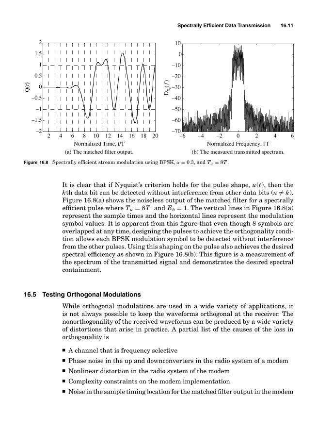
Spectrally Efficient Data Transmission 16.11
2 4 6 8 10 12 14 16 18 20–2
–1.5
–1
–0.5
0
0.5
1
1.5
2
Normalized Time, t/T
Q(t
)
(a) The matched filter output.
–6 –4 –2 0 2 4 6–70
–60
–50
–40
–30
–20
–10
0
10
Normalized Frequency, fT
Dx z(f
)
(b) The measured transmitted spectrum.
Figure 16.8 Spectrally efficient stream modulation using BPSK, α = 0.3, and Tu = 8T .
It is clear that if Nyquist’s criterion holds for the pulse shape, u(t), then thekth data bit can be detected without interference from other data bits (n �= k).Figure 16.8(a) shows the noiseless output of the matched filter for a spectrallyefficient pulse where Tu = 8T and Eb = 1. The vertical lines in Figure 16.8(a)represent the sample times and the horizontal lines represent the modulationsymbol values. It is apparent from this figure that even though 8 symbols areoverlapped at any time, designing the pulses to achieve the orthogonality condi-tion allows each BPSK modulation symbol to be detected without interferencefrom the other pulses. Using this shaping on the pulse also achieves the desiredspectral efficiency as shown in Figure 16.8(b). This figure is a measurement ofthe spectrum of the transmitted signal and demonstrates the desired spectralcontainment.
16.5 Testing Orthogonal Modulations
While orthogonal modulations are used in a wide variety of applications, itis not always possible to keep the waveforms orthogonal at the receiver. Thenonorthogonality of the received waveforms can be produced by a wide varietyof distortions that arise in practice. A partial list of the causes of the loss inorthogonality is
■ A channel that is frequency selective■ Phase noise in the up and downconverters in the radio system of a modem■ Nonlinear distortion in the radio system of the modem■ Complexity constraints on the modem implementation■ Noise in the sample timing location for the matched filter output in the modem
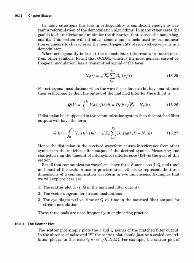
16.12 Chapter Sixteen
In many situations this loss in orthogonality is significant enough to war-rant a reformulation of the demodulation algorithms. In many other cases thegoal is to characterize and minimize the distortion that causes the nonorthog-onality. This section will introduce some common tools used by communica-tion engineers to characterize the nonorthogonality of received waveforms in ademodulator.
When orthogonality is lost at the demodulator this results in interferencefrom other symbols. Recall that OCDM, which is the most general case of or-thogonal modulation, has a transmitted signal of the form
Xz(t) =√
Eb
Kb∑l=1
Dz(l)sl(t) (16.25)
For orthogonal modulations when the waveforms for each bit have maintainedtheir orthogonality then the output of the matched filter for the kth bit is
Q(k) =∫ Tp
0Yz(t)s∗
l (t)dt = Dz(k)√
Eb + Nz(k) (16.26)
If distortion has happened in the communication system then the matched filteroutputs will have the form
Q(k) =∫ Tp
0Yz(t)s∗
l (t)dt =√
Eb
Kb∑l=1
Dz(l)g(k, l) + Nz(k) (16.27)
Hence the distortion in the received waveform causes interference from othersymbols in the matched filter output of the desired symbol. Measuring andcharacterizing the amount of intersymbol interference (ISI) is the goal of thissection.
Recall that communication waveforms have three dimensions (I, Q, and time)and most of the tools in use in practice are methods to represent the threedimensions of a communication waveform in two dimensions. Examples thatwe will explore here are
1. The scatter plot (I vs. Q in the matched filter output)
2. The vector diagram for stream modulations
3. The eye diagram (I vs. time or Q vs. time in the matched filter output) forstream modulation.
These three tools are used frequently in engineering practice.
16.5.1 The Scatter Plot
The scatter plot simply plots the I and Q points of the matched filter output.In the absence of noise and ISI the scatter plot should just be a scaled constel-lation plot as in this case Q(k) = √
EbDz(k). For example, the scatter plot of

Spectrally Efficient Data Transmission 16.13
–1.5 –1 –0.5 0 0.5 1 1.5–1.5
–1
–0.5
0
0.5
1
1.5
QI(k)
(k)
(a) Near ideal orthogonality.
–2 –1.5 –1 –0.5 0 0.5 1 1.5 2–2
–1.5
–1
–0.5
0
0.5
1
1.5
2
QI(k)
(k)
(b) Significant ISI.
Figure 16.9 Scatter plots for QPSK modulation.
a QPSK modulation when the amount of nonorthogonality is small is shownin Figure 16.9(a). A scatter plot for a case where some significant distortion ispresent in the received signal is shown in Figure 16.9(b). The ISI present in thematched filter output is manifested as a spreading of each of the constellationpoints. While the distortion shown in Figure 16.9(b) appears to not be signifi-cant enough to cause errors in the absence of noise it should be apparent thatthe addition of noise with this distortion will significantly degrade the errorrate performance. The scatter plot is a quick visual way for a communicationengineer to get a handle on the amount of nonorthogonality in a modulation.
An often used measure of distortion for communication engineers is the errorvector magnitude (EVM). The error vector for the matched filter output is de-fined to be Eq(k) = Q(k) − √
EbDz(k) and a vector diagram demonstrating thisconcept is shown in Figure 16.10(a). Communication engineers often quote thestatistic of EVM. EVM is the average error vector magnitude compared to thelargest normalized constellation point. There are many definitions of EVM butthe most often used definition is RMS-EVM. Precisely RMS-EVM is defined as
RMS-EVM =√∑Kb
l=1 |Eq(l)|2√
Kb maxi=0,...,M−1 |√Ebdi|(16.28)
and is most often reported in percentage. Most communication systems thatuse orthogonal modulations strive to achieve an EVM of less than 5%. Sys-tems which use large constellations (64QAM or 256QAM) like digital televisionoften have EVM requirements less than 3%. Most high performance vector an-alyzer type test equipment have automated EVM computations for commonmodulations used in accepted telecommunications standards. For example,Figure 16.10(b) shows an example test suite for a radio using one of the 64QAM

16.14 Chapter Sixteen
EbDz(k)
Q(k)
Eq(k)
Re(•)
Im(•
)(a) The error vector
1.5
Const
–1.5
300m/div
A: Ch1 OFDM Meas Range: 0 dBm
–2.707RBW: 312.5 kHz
2.7071Time Len: 40 Sym
Range: 0 dBm–10dBm
LogMag
10dB/div
Center: 70 MHzRBW: 17.3607 kHz
Span: 20 MHzTime Len: 220 uSec
20%
LinMag
0%
2%
/div
C: Ch1 OFDM Err Vect Spectrum Range: 0 dBm
Stop: 26 carrierTimeLen: 40 Sym
Start: –26 carrierRBW: 312.5 kHz
EVM = –30.302 dB EVM = 3.0541 %rmsPilot EVM = –32.465 dB CPE = 3.8536 %rms
Freq Err = 14.941 kHz IQ Offset = –55.59 dBSync Corr = 0.90418 Sym ClkErr = –6.54 ppmMod Fmt = 64 QAMOctets = 1200 Symbol = 45CodeRate = 3/4 Bit Rate = 54.000 Mbps
0 00000100 01010000 00010000 00010100 0100010120 01010100 0001 01 01000001 01010001 0100000140 01000101 01000100 00010001 01090C26 263A013E60 261E2138 0B142C22 00222E03 010F2324 2B2503
(b) A test suite for an 802.11a.
B: Ch1 Spectrum D: Ch1 OFDM Syms/Errs Range: 0 dBm
Figure 16.10 Testing using the error vector.
modes of operation for the IEEE 802.11a standard. Recall as discussed earlier802.11a is an OFDM based wireless modem and this figure shows a scatterplot for all subcarrier matched filter outputs, the received signal spectrum, andcomputations on the error vector for each subcarrier. This test suite is auto-matically produced by an Agilent vector signal analyzer and a great deal ofinformation can be derived from this plot about the performance of a communi-cation system using orthogonal modulation. For example, a very useful tutorialarticle on how to use EVM to troubleshoot an orthogonal modulation systemis [Agi00].

Spectrally Efficient Data Transmission 16.15
16.5.2 Stream Modulations
Since historically stream modulations have seen the most utility in practiceseveral techniques have evolved to test the performance of orthogonal streammodulations. The two most common tests in stream modulation are the vectordiagram plot and the eye diagram.
Vector Diagram
A generalization of the scatter plot is the vector diagram. The vector diagramwas introduced in Chapter 4 as a way to visualize the 3D characteristics of thecomplex envelope in a 2D graph. For orthogonal stream modulation as withany IQ modulation the vector diagram can be used to get information aboutthe vector modulated signal. For example, Figure 16.11 shows the transmittedvector diagram for a QPSK modulated stream modulation with a spectral co-sine pulse with α = 0.3 and Tu = 8T . A particular important vector diagram isthe output of the matched filter to the transmitted pulse shape. This vectordiagram with near ideal orthogonality should go through the constellationpoints at each sample time. Often in a vector diagram of the matched filteroutput, these sample times are marked with a different marker to empha-size these sample times. For example, for a QPSK modulated stream modula-tion with a spectral cosine pulse with α = 0.3 and Tu = 8T with little loss
–2 –1.5 –1 –0.5 0 0.5 1 1.5 2–2
–1.5
–1
–0.5
0
0.5
1
1.5
2
xI(t)
x Q(t
)
Figure 16.11 Vector diagram for a transmitted signal with QPSK, α = 0.3 and Tu = 8T .

16.16 Chapter Sixteen
–2 –1.5 –1 –0.5 0 0.5 1 1.5 2–2
–1.5
–1
–0.5
0
0.5
1
1.5
2
QI(t)
(t)
(a) Near ideal orthogonality
–2 –1.5 –1 –0.5 0 0.5 1 1.5 2–2
–1.5
–1
–0.5
0
0.5
1
1.5
2
QI(t)
(t)
(b) Significant ISI
Figure 16.12 Matched filter output vector diagrams for a stream modulation with a spectral cosine pulse withα = 0.3 and Tu = 8T . Sample times of the matched filter output are denoted with a circle.
in orthogonality the vector diagram of the matched filter output is shown inFigure 16.12(a). Note that the matched filter output samples taken by them-selves would be the scatter plots shown in Figure 16.9. Distortion of the streammodulation signal will produce significant ISI and a vector diagram for a case ofsignificant ISI is shown in Figure 16.12(b). Vector diagrams for stream modula-tions give engineers insights into the performance of practical implementationsof orthogonal stream modulation.
The Eye Diagram
The eye diagram is a technique to view the time waveforms out of the matchedfilter. Again the matched filter output is a 3D signal and the eye diagram isa method to visualize this 3D signal in two dimensions. The eye diagram isa repetitive plot of the matched filter output (either I or Q channel) over onesymbol in time of the stream modulation. An example of the eye diagram forthe case of near ideal orthogonality is shown in Figure 16.13(a). The originalmethod of producing an eye diagram goes back to the early days of digitalcommunication when analog oscilloscopes were the primary time domain anal-ysis tool available to a communication engineer. The I or Q channel of thematched filter output could be connected to the oscilloscope and the symbolclock could be used as the trigger and an eye diagram would then be visible onthe display. The eye diagram shows the possible transitions from one symbol tothe next and how impacted the orthogonality is by any distortion. An exampleof the eye diagram for the case of significant ISI is shown in Figure 16.13(b). TheISI causes the space between the worst case sample points of the matched filteroutputs to move closer to the decision threshold. In the case of BPSK modulationas shown in Figure 16.13 the threshold will be zero. This effect of the ISI movingthe optimum sample point closer to the decision boundary is often referred to as

Spectrally Efficient Data Transmission 16.17
–0.5 –0.4 –0.3 –0.2 –0.1 0 0.1 0.2 0.3 0.4 0.5–2
–1.5
–1
–0.5
0
0.5
1
1.5
2
Normalized Time, t/T
QI(
t)
(a) Near ideal orthogonality
–0.5 –0.4 –0.3 –0.2 –0.1 0 0.1 0.2 0.3 0.4 0.5–2
–1.5
–1
–0.5
0
0.5
1
1.5
2
Normalized Time, t/T
QI(
t)
(b) Significant ISI
Figure 16.13 Matched filter output eye diagrams for a spectral cosine pulse with α = 0.3 and Tu = 8T . BPSKmodulation.
the “closing” of the eye. A communication system is often referred to as havinga closed eye if there are some ISI patterns which would cause a deterministicerror to occur in the simple threshold test demodulator of orthogonal demodula-tors. Most communications system analysis tools have the capability to produceeye diagrams and vector plots since they prove useful to communication engi-neers. For example, Matlab has an eyediagram command. The Agilent vectoranalyzer can produce eye diagrams for most standard stream modulations andan example of both an eye diagram and a vector diagram for a 16QAM streammodulation is shown in Figure 16.14. The tools of the eye diagram and the
(a) (b)
Figure 16.14 Test results for an orthogonal stream modulation from an Agilent vector signal analyzer. 16QAM withα = 0.25.

16.18 Chapter Sixteen
vector plot produce a great deal of insight into the implementation of orthogonalstream modulations and are often used by communication system engineers.
16.6 Conclusions
This chapter has looked at some practical aspects of digital communicationsusing orthogonal modulations. Techniques to shape the spectrum of orthogonalmodualtions in response to requirements often mandated in real implemen-tations were overviewed. The concept of the cosine pulse that is popular inpractice was introduced. How this cosine pulse can be used in orthogonal mod-ulations was briefly summarized. Finally, a brief overview of tools used in theindustry to characterize orthogonal modulations was given. Understanding theconcepts in this chapter will help the student get closer to understanding howdigital communications is implemented in modern systems.
16.7 Homework Problems
Problem 16.1. Prove
Vu(mT ) ={
Eu m = 00 elsewhere
(16.29)
if and only if
k=∞∑k=−∞
Gu
(f + k
T
)= T Eu (16.30)
Hint: Note the proof is based on Nyquist sampling theorem. This property in-dicates ways to design other pulses besides the spectral cosine pulse family tosatisfy the Nyquist’s criteria for zero ISI.
Problem 16.2. Prove the smallest bandwidth (100% of energy is contained withinthis bandwidth) that can be achieved in linear stream modulation is BT = 1/Twhen Dz(k) can have an arbitrary constellation. If Dz(k) is restricted to be realvalued show the bandwidth can be BT = 1/(2T ).
Problem 16.3. Prove that usc(t) = F−1{Usc(f )}.Problem 16.4. The company you work for, Horizon Wireless, has purchased 1 MHzof spectrum from the federal government of Elbonia. The marketing group ofHorizon Wireless in Elbonia has decided that the way to make money in Elboniais to divide the purchased spectrum into 20 equal size channels (of 50 kHz) andsell radios that use these 20 channels to the Elbonian government for use bytheir diplomatic corp.
(a) Give an example of a modulation that will achieve a 40 kHz transmissionrate in a spectrally efficient and power efficient manner on one of these

Spectrally Efficient Data Transmission 16.19
Gu1( f ) Gu2
( f ) Gu3( f )
A1 A2
A3
2A3
12T− 1
2Tf f f1
T1T−1
T1T−
Figure 16.15 The energy spectrum of three possible pulses for linear streammodulation.
channels while sending packets of Kb = 256 bits and achieving a demodu-lation complexity that is reasonably close to O(256).
(b) Give an example of a modulation that will achieve a 120 kHz transmissionrate in a spectrally efficient and power efficient manner on one of these chan-nels while sending packets of Kb = 768 bits and achieving a demodulationcomplexity that is reasonably close to O(768).
(c) Assume the propagation loss in the channel is Lp = aR−2 where R is therange of communication and a is a constant and the transmitted powerremains the same for both transmission rates. If your design in part (a)can achieve a range of 1 km with a low frame error rate, what range willyour design in (b) achieve and give the same frame error rate performance.(assume the noise stays constant).
Problem 16.5. The energy spectrum of three pulse shapes that can be used ina linear stream modulation is shown in Figure 16.15. Recall linear streammodulation has the form
Xz,i(t) =√
Eb
Kb∑l=1
Dz(l)ui(t − (l − 1)T ) (16.31)
where ui(t) corresponds to one of the three possible pulse shapes.
(a) Find the amplitude Ai for i = 1, 2, 3 such that Eu = 1.
(b) Prove that each of these three pulses can be used in a stream modulationand have simple bit demodulation result. Hint: These pulses have the samecharacteristic as the squared cosine pulse that makes the squared cosinepulse shape useful for stream modulation.
(c) Find the form of u3(t).
(d) Which pulse shape will provide the best spectral efficiency if the measureof bandwith is the 10 dB bandwidth, B10?
Problem 16.6. Your boss has tasked you with designing an OFDM cable modemto send packets of Kb = 256 bits in less than 300 µs achieving a data rate

16.20 Chapter Sixteen
Wb ≥ 853.3 kHz. She wants you to use less than 1 MHz of spectrum and causelittle interference to transmissions from adjacent houses (each house is fre-quency multiplexed). The cable is assumed to be a frequency flat device andthe goal given by your boss is to have a simple demodulator. Specify all theimportant parameters and pulse shapes.
Problem 16.7. The eye diagram for BPSK shown in Figure 16.13 has two levels atthe optimum sample point. How many levels would the optimum sample pointhave in an eye diagram for
(a) QPSK modulation.
(b) 8PSK modulation.
(c) the 8-ary linear modulation introduced in Example 15.1.
(d) 16QAM introduced in Problem 15.1.
Problem 16.8. In your current job assignment you are expected to find theimpact of imperfections in the hardware to be used to build your commu-nication systems. The previous engineer who worked on the assignment had de-rived the impact of a amplitude imbalance in the I/Q upconverter (seeProblem 4.25)
xz(t) = AxI (t) + j BxQ(t) =√
21 + γ
xI (t) + j
√2γ
1 + γxQ(t) (16.32)
where the amplitude imbalance is γ and the impact of a phase imbalance of θ
in the I/Q upconverter (see Problem 4.13)
xz(t) = xI (t) − xQ(t) sin(θ) + j xQ(t) cos(θ ) (16.33)
(a) Derive the overall response to an amplitude imbalance of γ and a phaseoffset of θ .
(b) Assume a linear modulation is used, xz(t) = Dzu(t) = (DI + j DQ)u(t) showthat the error vector magnitude is given as
EVM(DI , DQ, θ , γ )
=√
(1 − A)2 D2I + 2(1 − A)B sin(θ )DI DQ + (1 − 2B cos(θ ) + B2)D2
Q
Problem 16.9. The government has given the company SpyRUs 5 MHz of band-width to bring down video surveillence images of Odillian terrorist cells froma satellite. The video requires a data rate of 12 Mbits/s and video is dividedup into packets of 1024 bits. The adjacent spectrum is being used for an ESPNbroadcast of the Ohio State versus Michigan football game and cannot be dis-turbed (there must be at least 50 dB of attenuation in the adjacent 5 MHzchannels or ESPN by contract can fine SpyRUs).

Spectrally Efficient Data Transmission 16.21
0.5 1.0−0.5−1.0
0.5
f
2.0
1.5
Gu( f )
Figure 16.16 The rocket signal infrequency.
(a) The satellite channel is well modeled as frequency flat with an AWGN with aone-sided spectral density of N0. Design a packet transmission system thatwill work for SpyRUs. Specify in detail how the 1024 bits will be transmittedand the precise data rate of the design.
(b) Assume the loss in the channel is Lp, in your model specify the normaliza-tion constants such the energy per bit is Eb.
(c) Estimate the error rate in demodulation for a given Eb/N0.
Problem 16.10. (RW) An interesting characteristic of the Fourier transform islinearity and linearity can be used to compute the Fourier transform of compli-cated functions by decomposing these function into sums of simple functions.
(a) Prove if y(t) = x1(t) + x2(t) that Y (f ) = X1(f ) + X2(f ).
(b) For the pulse shape spectrum given in Figure 16.16 find a symbol rate atwhich the Nyquist’s criterion will be satisfied.
Problem 16.11. Show that the rectangular pulse, i.e.,
ur (t) =
⎧⎪⎨⎪⎩√
1T
0 ≤ t ≤ T
0 elsewhere
(16.34)
satisfies the condition given in Eq. (16.30).
Problem 16.12. (Design Problem) Specify and identify all components of thetransmitted waveform for a stream modulation that has a transmission rateof Wb = 100 kbits/s, uses BPSK modulation, achieves a spectral efficiency ofηB = 0.75 where BT is the 30 dB bandwidth of the transmitted signal, andhas an optimum demodulator with a complexity that scales linearly with thenumber of bits transmitted.

16.22 Chapter Sixteen
Problem 16.13. Often in communications a system requirement is that a certainpercentage of the total power or energy must lie within a certain bandwidthfor the system to be acceptable. For stream modulation using ideal an spectralcosine pulse, plot the 95% energy per bit bandwidth as a function of α. Usingthese results propose a bit rate for a binary stream modulation that can beachieved where 95% of the energy per bit lies within 1 MHz of bandwidth.
16.8 Example Solutions
Problem 16.2. Nyquist’s criterion for stream modulation is
0 = [Dz(l)D∗z (k)Vu((k − l)T )] (16.35)
so for a complex constellation this becomes Vu(mT ) = 0 for m �= 0. UsingProblem 16.1 it is clear that the pulse used must satisfy
k=∞∑k=−∞
Gu
(f + k
T
)= T Eu (16.36)
Hence if the pulse spectrum is
Gu(f ) ={
T Eu | f | ≤ 12T
0 elsewhere(16.37)
the condition is satisfied and BT = 1/T . If the bandwidth becomes smallerthan BT = 1/T then the condition in Eq. (16.36) will not hold.
For a real-valued constellation with Vu(mT ) = VuI (mT ) + j VuQ(mT ) therequirement becomes VuI (mT ) = 0. Note from Chapter 4 that
Gu(f ) = GuI (f ) + j GuQ(f ) GuI = Gu(f ) + G∗u(− f )
2(16.38)
Using the results from Problem 16.1 the condition that must hold is
k=∞∑k=−∞
GuI
(f + k
T
)= T Eu (16.39)
A pulse spectrum of
Gu(f ) ={
2T Eu 0 ≤ f ≤ 12T
0 elsewhere(16.40)
will satisfy Eq. (16.39) and provide a bandwidth of BT = 12T .
Problem 16.4.
(a) There are a multitude of modulations that can achieve this specification of0.8 bits/s/Hz. For example, you could use stream modulation with BPSK

Spectrally Efficient Data Transmission 16.23
modulation, a symbol rate of 40 kHz (T = 25 µs) and a spectral cosinepulse with α < 0.25.
(b) There are a multitude of modulations that can achieve this specificationof 2.4 bits/s/Hz. For example, you could use stream modulation with 8PSKmodulation, a symbol rate of 40 kHz (T = 25 µs) and a spectral cosine pulsewith α < 0.25.
(c) For the examples considered in (a) and (b) the word error probability isgiven in Figure 14.8. The difference in the required Eb/N0 for BPSK and8PSK at medium to high SNR is about 3.5 dB. Since the transmitted poweris the same in both cases, the received signal power will be PRz = L2
p PXz .The received energy per bit in each case is
Eb(BPSK) = PRz T Eb(8PSK) = PRz T /3 (16.41)
It is clear here that the received energy per bit is lower with the highertransmission rate and also the required Eb/N0 for 8PSK is larger hencethe second transmission scheme will be doubly penalized, i.e.,
PRz(8PSK) = 3(100.35)PRz(BPSK) = 6.72PRz(BPSK) (16.42)
Consequently, the range of transmission for 8PSK will be
R(8PSK) = (6.72)0.25 R(BPSK) = 0.62R(BPSK) (16.43)
16.9 Miniprojects
Goal: To give exposure
■ to a small scope engineering design problem in communications.■ to the dynamics of working with a team.■ to the importance of engineering communication skills (in this case oral pre-
sentations).
Presentation: The forum will be similar to a design review at a company(only much shorter). The presentation will be of 5 minutes in length with anoverview of the given problem and solution. The presentation will be followedby questions from the audience (your classmates and the professor). All teammembers should be prepared to give the presentation.
16.9.1 Project 1
Project Goal: This project examines the design of a realistic pulse shape to beused with linear modulation that will meet a spectral emissions mask.
A spectral emissions mask is given in Figure 16.17. This spectral emissionsmask is the one used for GSM handsets. So this problem is one of great practical

16.24 Chapter Sixteen
–80
–70
–60
–50
–40
–30
–20
–10
0
0 100 200 300 400 500 600 700 800
Rel
ativ
e E
mis
sion
s L
evel
, dB
Frequency Offset, kHz
Figure 16.17 Spectral emissions mask for a GSM mobile.
interest. Consider a linear stream modulation having the form
Xz(t) =√
Eb
Kb∑k=1
Dz(k)u(t − (k − 1)T ) (16.44)
The design is further constrained in that the pulse, u(t), must not extend forlonger than Tu = 40 µs in time. Design a pulse shape that will satisfy Nyquist’scriterion for an arbitrary constellation.
For the remainder of the project it is assumed that the pulse shape designedabove is used with BPSK modulation. Any finite length pulse shape whichachieves this spectral mask will have to produced some intersymbol interfer-ence (ISI) (i.e., Nyquist’s criterion cannot exactly be met). Hence the matchedfilter demodulator given in Figure 16.18 will not be exactly optimal but can bemade to be very close to optimal with a well designed pulse shape.
+−u*(Tu – t)
Tu + (k – 1)T
QI(k)Re[•] I(k)Yz(t)
Figure 16.18 The baseband demodulator for binary pulse amplitude modu-lation.
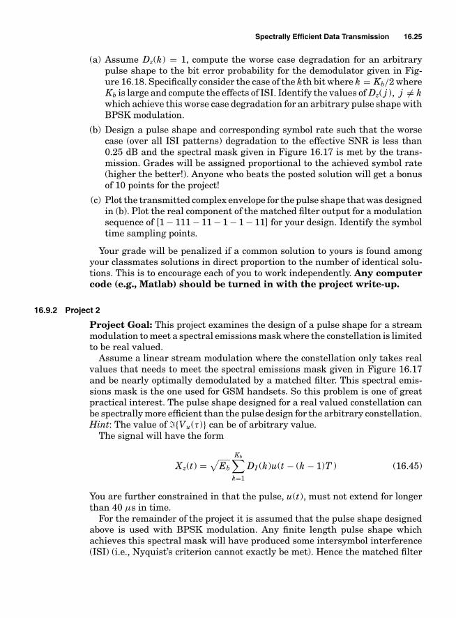
Spectrally Efficient Data Transmission 16.25
(a) Assume Dz(k) = 1, compute the worse case degradation for an arbitrarypulse shape to the bit error probability for the demodulator given in Fig-ure 16.18. Specifically consider the case of the kth bit where k = Kb/2 whereKb is large and compute the effects of ISI. Identify the values of Dz( j ), j �= kwhich achieve this worse case degradation for an arbitrary pulse shape withBPSK modulation.
(b) Design a pulse shape and corresponding symbol rate such that the worsecase (over all ISI patterns) degradation to the effective SNR is less than0.25 dB and the spectral mask given in Figure 16.17 is met by the trans-mission. Grades will be assigned proportional to the achieved symbol rate(higher the better!). Anyone who beats the posted solution will get a bonusof 10 points for the project!
(c) Plot the transmitted complex envelope for the pulse shape that was designedin (b). Plot the real component of the matched filter output for a modulationsequence of [1 − 111 − 11 − 1 − 1 − 11] for your design. Identify the symboltime sampling points.
Your grade will be penalized if a common solution to yours is found amongyour classmates solutions in direct proportion to the number of identical solu-tions. This is to encourage each of you to work independently. Any computercode (e.g., Matlab) should be turned in with the project write-up.
16.9.2 Project 2
Project Goal: This project examines the design of a pulse shape for a streammodulation to meet a spectral emissions mask where the constellation is limitedto be real valued.
Assume a linear stream modulation where the constellation only takes realvalues that needs to meet the spectral emissions mask given in Figure 16.17and be nearly optimally demodulated by a matched filter. This spectral emis-sions mask is the one used for GSM handsets. So this problem is one of greatpractical interest. The pulse shape designed for a real valued constellation canbe spectrally more efficient than the pulse design for the arbitrary constellation.Hint: The value of �{Vu(τ )} can be of arbitrary value.
The signal will have the form
Xz(t) =√
Eb
Kb∑k=1
DI (k)u(t − (k − 1)T ) (16.45)
You are further constrained in that the pulse, u(t), must not extend for longerthan 40 µs in time.
For the remainder of the project it is assumed that the pulse shape designedabove is used with BPSK modulation. Any finite length pulse shape whichachieves this spectral mask will have produced some intersymbol interference(ISI) (i.e., Nyquist’s criterion cannot exactly be met). Hence the matched filter

16.26 Chapter Sixteen
demodulator given in Figure 16.18 will not be exactly optimal but can be madeto be very close to optimal with a well-designed pulse shape.
(a) Assume Dz(k) = 1, compute the worse case degradation for an arbitrarypulse shape to the bit error probability for the demodulator given inFigure 16.18. Specifically consider the case of the kth bit where k = Kb/2where Kb is large and compute the effects of ISI. Identify the values ofDz( j ), j �= k which achieve this worse case degradation for an arbitrarypulse shape with BPSK modulation.
(b) If u1(t) = u(t) exp[ j 2π fot], find Vu1 (τ ). This result can help you design aninfinite support pulse from the pulse shapes introduced in the text for usewith real valued linear stream modulation.
(c) Design a pulse shape and corresponding symbol rate such that the worsecase (over all ISI patterns) degradation to the effective SNR is less than0.25 dB and the spectral mask given in Figure 16.17 is met by the trans-mission. Grades will be assigned proportional to the achieved symbol rate(higher the better!). Anyone who beats the posted solution will get a bonus of10 points for the project!
(d) Plot the transmitted complex envelope for the pulse shape designed in (c).In addition, plot the real component of the matched filter output for a mod-ulation sequence of [1 − 1 1 1 − 1 1 − 1 − 1 − 1 1] for your design. Identifythe symbol time sampling points.
Your grade will be penalized if a common solution to yours is found among yourclassmates solutions in direct proportion to the number of identical solutions.This is to encourage each of you to work independently. Any computer code(e.g., Matlab) should be turned in with the project write-up.
16.9.3 Project 3
Project Goal: To examine a typical degradation that occurs in an orthogonalmodulation in a real system.
An OFDM signal is to be received that is transmitting Kb = 16 bits with1 bit on each subcarrier, has a carrier frequency of fc = 1800 Hz, and achievea transmission rate of Wb = 2000 Hz. Unfortunately, the frequency sources atthe transmitter and receiver cannot be perfectly synchronized so that
Yz(t) = Xz(t) exp[ j 2π fot] + Wz(t) (16.46)
where fo is the resulting frequency offset and
Xz(t) =
⎧⎪⎪⎪⎨⎪⎪⎪⎩
Kb∑l=1
Dz(l)
√Eb
Tpexp[ j 2π fd (2l − Kb − 1)t] 0 ≤ t ≤ Tp
0 elsewhere
(16.47)

Spectrally Efficient Data Transmission 16.27
It is desired to still use approximately the same demodulator as in the case ofno frequency offset, i.e.,
[
H ∗(k, k)∫ Tp
0Yz(t)
√1
Tpexp[− j 2π fd (2k − Kb − 1)t]dt
]
= [H ∗(k, k)Q(k)]
I (k)=0>
<I (k)=1
0 (16.48)
This demodulator will have ISI because the orthogonality condition does nothold.
(a) Show that
Q(k) =Kb∑l=1
H (l, k)Dz(l) + Nz(k) (16.49)
and identify H (l, k).
(b) For k = 8 plot a scatter plot of Q(k) for fo = 0, 1, 10 Hz with Nz(k) = 0.
(c) For k = 8 compute the value of fo that will result in less than a 3%RMS-EVM. Ensure that the amplitude loss of the desired signal due tothe frequency offset is accounted for before computing the EVM.
16.9.4 Project 4
Project Goal: To examine a typical degradation that occurs in an orthogonalmodulation in a real system.
A stream modulated signal is to be received that is transmitting Kb = 16bits with a carrier frequency of fc = 1800 Hz, and achieves a transmission rateof Wb = 2000 Hz. Unfortunately, the frequency sources at the transmitter andreceiver cannot be perfectly synchronized so that
Yz(t) = Xz(t) exp[ j 2π fot] + Wz(t) (16.50)
where fo is the resulting frequency offset and
Xz(t) =
⎧⎪⎨⎪⎩
Kb∑l=1
Dz(l)u(t − (l − 1)T ) 0 ≤ t ≤ Tp
0 elsewhere
(16.51)

16.28 Chapter Sixteen
It is desired to still use approximately the same demodulator as in the case ofno frequency offset, i.e.,
[
H ∗(k, k)∫ Tp
0Yz(t)u ∗ (t − (k − 1)T )dt
]= [H ∗(k, k)Q(k)]
I (k)=0>
<I (k)=1
0
(16.52)
This demodulator is suboptimal and will have ISI because the orthogonalitycondition does not hold in the matched filter outputs due to the frequency offset.
(a) Show that
Q(k) =Kb∑l=1
H (l, k)Dz(l) + Nz(k) (16.53)
and identify H (l, k).
(b) For k = 8 plot a scatter plot of Q(k) for fo = 0, 1, 10 Hz with Nz(k) = 0.
(c) For k = 8 compute the value of fo that will result in less than a 3% RMS-EVM. Ensure that the amplitude loss of the desired signal due to the fre-quency offset is accounted for before computing the EVM.

Chapter
17Orthogonal Modulations with
Memory
17.1 Canonical Problems
Up to this point in this text we have introduced two general methods to com-municate Kb bits.
1. General M-ary modulations
■ The advantage of a general M-ary modulation is that it can achievevery good fidelity and arbitrary spectral efficiency.
■ The disadvantage is that without more structure the optimal demodu-lator has complexity O(2Kb).
2. Orthogonal memoryless modulations (including stream modulations, OFDM,OCDM)
■ The advantage of orthogonal modulation is that the optimum demod-ulator has complexity O(Kb) and a desired spectral efficiency can beachieved with a proper design of the modulation signals.
■ The disadvantage is that the fidelity of message reconstruction is lim-ited to that of binary modulations and this performance is far fromShannon’s limit.
The goals for the final chapter of the text will be to explore the remaining areasof trade-off in fidelity, complexity, and spectral efficiency, i.e.,
■ Improving the demodulation fidelity or spectral characteristics of orthogonalmodulations with a goal of maintaining a demodulation complexity that isO(Kb).
17.1
Copyright © 2007 by The McGraw-Hill Companies. Click here for terms of use.

17.2 Chapter Seventeen
Shannon has given us an upperbound on the performance that can be achievedfor a given spectral efficiency (see Figure 12.5) and there are a variety of waysto approach that performance with a demodulation complexity that is O(Kb).The concept of orthogonal modulations with memory are what have allowedcommunication theory to approach the bounds provided by Claude Shannon inhis ground breaking work on information theory [Sha48]. This chapter will bea brief introduction into the topic and an examination of the implications ofadding memory to the performance and the spectral characteristics.
17.2 Orthogonal Modulations with Memory
This section addresses a class of communication problems where an orthog-onal modulation is implemented with the modulation symbols having mem-ory. The memory is normally included in the modulation to either improve thefidelity of demodulation or change the spectral characteristics of a memory-less orthogonal modulation. This type of modulation is referred to as modula-tion with memory (MWM) and incorporates most error control coding schemes[Wic95, LC04, BDMS91]. Our goal in this text is not to explore how to designthese MWM but to understand the communication theory behind the fidelity,spectral efficiency, and the demodulation complexity. Design of MWM is oftenaddressed in a course on error control coding. Suffice it to say here that a MWMadds memory to the modulation process with a goal of either changing the spec-tral characteristics of the transmitted signal or improving the resulting squaredEuclidean distance spectrum.
This chapter first considers the special case of an orthogonal modulation withmemory (OMWM) where 1 bit is sent with each symbol or orthogonal dimen-sion. For simplicity of discussion this section will again assume that the bitsto be transmitted are equally likely and independent. The generalizations forcorrelated bits is possible but the added notational complexity is not worth thegain in generality. The resulting data symbols can then be transmitted usingan orthogonal modulation. The data modulation symbols, Dz(l), are due to thestream of information bits, I (l), l = 1, . . . , Kb. The tilde notation will be used todifferentiate between modulations that have memory (tilde) and memorylessmodulations (not tilde). For continuity with the previous discussions on orthogo-nal modulations this initial discussion considers exclusively modulations wherethe transmission bit rate is R = 1 bit per symbol. To keep a consistent normal-ization the mapping, Dz(l) = a(J (l)), is selected such that E[|Dz(l)|2] = 1. Thetransmitted signal will have the form
Xz(t) =Nf∑l=1
Dz(l)sl(t) (17.1)
where Nf is the length of the transmitted frame in symbols and sl(t) are theorthogonal basis functions (spreading waveforms) used to transmit the symbols.

Orthogonal Modulations with Memory 17.3
I(l)J(l)
σ(l)
z−1
Finite State Machine
M-aryOrthogonalModulator
Xz(t)σ(l + 1)
Figure 17.1 The block diagram for a modulation with memorywith a transmission rate of 1 bit per symbol.
Note, this formulation is equally applicable to being used in OCDM, OFDM, ora stream modulation. A more general formulation for orthogonal modulationswhere the rate is not constrained to be 1 bit per symbol is considered later inthis chapter.
An orthogonal modulation with memory, as considered in this section, con-sists of a finite state machine operating at the symbol rate where the output ofthe finite state machine is used as an input to an Ms-ary orthogonal modula-tion. Figure 17.1 shows the block diagram for a linear orthogonal modulationwith memory. At each symbol time a new bit, I (l) is input into the systemand this produces a new constellation label, J (l), and a new modulation state,σ (l+1). Let Ns denote the number of states in the modulation and the nonlinearequations governing the finite state machine are given as
σ (l + 1) = g1(σ (l), I (l)) (17.2)
J (l) = g2(σ (l), I (l)) (17.3)
For notational purposes denote the set of all possible state values as �σ . Ingeneral, it is desirable to have νc extra symbols transmitted to return the mod-ulation to a common final state at the end of the transmission frame. Again thetotal length of the frame for the orthogonal modulation is denoted Nf , hence,in this case when R = 1 bit/symbol Nf = Kb + νc, where νc is a modulationdependent constant. This return to a final common state is most often known astermination in the literature of MWM [Wic95, LC04, BDMS91]. Note that theeffective rate is Reff = Kb
Kb+νc< 1 but if a large number of bits are transmitted
then the loss in efficiency by including the termination becomes small.A couple comments about OMWM are appropriate at this point. An OMWM
can only provide an improvement in demodulation fidelity or a change in spec-tral characteristics compared to a memoryless modulation if there is some re-dundancy to be exploited. An orthogonal modulation with memory has 2Kb pos-sible bit sequences as an input. The modulation symbols being mapped ontothe orthogonal modulation have MKb+νc
s possible realizations. Hence if there isto be redundancy that the OMWM can exploit for large Kb then Ms > 2. Theimproved fidelity of demodulation or spectral efficiency is achieved by pickingthe best M = 2Kb possible transmitted symbol sequences out of the MKb+νc
s total

17.4 Chapter Seventeen
possible transmitted symbol sequences. Secondly, the more states an OMWMhas the more memory it contains. In general, more memory allows a designerto make better choices in the transmitted symbol sequences but at a cost of ahigher complexity demodulation. Finally, an OMWM is often represented witha directed graph [Wes01]. The vertices of the directed graph represent the stateof the modulation at a particular time and the edges of the directed graph repre-sent the allowable transitions between states. In the communications literaturethe directed graph is often referred to as a trellis. Because of this trellis repre-sentation OMWM are often referred to as trellis coded modulation (TCM). Thistrellis representation of an OMWM is explored in the example considered inthe next section.
17.2.1 MLWD for Orthogonal Modulations with Memory
Recall OMWM can be characterized with a finite state machine defined with
σ (l + 1) = g1(σ (l), I (l)) (17.4)
J (l) = g2(σ (l), I (l)) (17.5)
The equivalent modulation symbol is Dz(l) = a(J (l)) with a(•) being theconstellation mapping. Here we examine only the optimum word demodulation(MLWD). The optimum word demodulator is still the MLWD for an orthogo-nal modulation except now the memory of the modulation must be accountedfor when computing the maximum likelihood metric. Due to the orthogonalmodulation the MLWD has
�I = arg maxi=0,...,M−1
T i
= arg maxi=0,...,M−1
√Eb
Nf∑k=1
[d ∗i (k)Q(k)] − Eb
2
Nf∑k=1
|d i(k)|2
= arg mini=0,...,M−1
Nf∑k=1
|Q(k) −√
Ebd i(k)|2 (17.6)
where Q(k) is the matched filter ouptut sample. Consequently, the output of theMLWD can be thought of as the possible transmitted modulation symbols (con-strained by the modulation with memory) that is closest in Euclidean distanceto the matched filter outputs that are observed (Q(k)) over the entire frame(k = 1, Nf ). This minimum squared Euclidean distance decoder provides anice analogy to the demodulation of memoryless orthogonal modulations.
As with a general M-ary modulation, the achieved fidelity in demodulationof the MLWD for an OMWM is determined by the squared Euclidean distancespectrum. Due to the use of an orthogonal modulation the squared Euclidean

Orthogonal Modulations with Memory 17.5
distance between any two words is given as
�E (i, j ) =∫ ∞
−∞|xi(t) − xj (t)|2dt = Eb
∫ ∞
−∞
∣∣∣∣∣∣Nf∑l=1
sl(t)[d i(l) − dj (l)]
∣∣∣∣∣∣2
dt
= Eb
Nf∑l=1
Nf∑k=1
(d i(l) − dj (l))(d i(k) − dj (k))∗∫ ∞
−∞sl(t)s∗
k(t)dt (17.7)
= Eb
Nf∑l=1
|d i(l) − dj (l)|2 (17.8)
Consequently, the important characteristics in terms of fidelity of demodulationof an OMWM is the squared Euclidean distance between the code sequencesproduced by the modulation with memory. Consequently, the performance ofthe OMWM is only a function of the finite state machine that characterizes themodulation. For a R = 1, an improved demodulation fidelity will be achievedcompared to a memoryless orthogonal modulation if the minimum Euclideansquared distance of the modulation with memory is greater than the bestEuclidean squared distance for a R = 1 memoryless modulation. The bestR = 1 memoryless modulation (BPSK) achieves a Euclidean squared distanceof �E,min = 4Eb so this value will be our benchmark for comparison.
17.2.2 An Example OMWM Providing Better Fidelity
Consider an OMWM consisting of a four state trellis code (Ns = 4) using 4PAMmodulation (Ms = 4) as proposed by Ho, Cavers, and Varaldi [HCV93]. It shouldbe noted here that this OMWM is a simple construction using a general com-bined modulation and coding technique proposed by Ungerboeck in [Ung82].This example OMWM illustrates some important properties that will becomeapparent in the sequel. The modulation updates are given in Table 17.1. Herewe have �σ = {1, 2, 3, 4}. Note that the modulation is normalized to have anaverage energy of unity. The trellis for this modulation is shown in Figure 17.2.As mentioned before, the vertices of the trellis diagram represent the states ateach time interval (hence for this code there are Ns = 4 vertices at each pointin time) and the edges are the possible transitions (note for instance σ (l) = 1
TABLE 17.1 The finite state machine description of an example trellis code
σ (l + 1) = g1(I (l), σ (l)) J (l) = g2(I (l), σ (l)) Dz(l) = a(J (l))
I (l) I (l) J (l) Dz(l)
State, σ (l) 0 1 State, σ (l) 0 1 0 −3/√
5
1 1 2 1 0 2 1 −1/√
52 3 4 2 3 1 2 1/
√5
3 1 2 3 2 0 3 3/√
54 3 4 4 1 3

17.6 Chapter Seventeen
I(k) = 0 I(k) = 1
−3/ 5
5
5
5
1/ 5
5
5
3/ 5
σ(l) = 1 σ(l + 1) = 1
σ(l + 1) = 2
σ(l + 1) = 3
σ(l + 1) = 4
σ(l) = 2
σ(l) = 3
σ(l) = 4
σ (l) σ(l + 1)
3/
1/
−1/
−3/
−1/
Figure 17.2 The trellis diagram of the Ho, Cavers, and Varaldi trellis code.
can only transition to σ (l+1) = 1 and σ (l+1) = 2). There are a total of 2Ns = 8edges in this example. It should be noted that the trellis labels in this text willbe put to the side as in Figure 17.2. The edge labels indicate the input, I (k), thatcauses the transition and the modulation symbol that is output for that inputand state. Unless noted all the upper transitions in a trellis will correspond tothe input I (k) = 0. As is the case for orthogonal modulation the normalizationis set as
E[|Dz(l)|2
] = R = 1 (17.9)
For instance, when σ (l) = 1 and I (l) = 0 the output symbol is Dz(l) = −3/√
5.This particular code requires at most two transitions to allow the modulationto transition from any state to any other state so this code has νc = 2. Forinstance, if σ (l) = 2 then to get to σ (l + 2) = 1 one would have to transition toσ (l+1) = 3 first. Alternatively if σ (l) = 1 then we could immediately transitionto σ (l + 1) = 1.
Nf trellis sections can be combined together to get a complete description ofan OMWM. For instance for Kb = 4, Figure 17.3 shows a trellis description for amodulation that has σ (1) = 1 and returns to σ (7) = 1. One can verify that thereare 2Kb paths through this trellis. To understand the fidelity of demodulation
Figure 17.3 The trellis diagram of the Ho, Cavers Varaldi trellis code. Kb = 4.

Orthogonal Modulations with Memory 17.7
0 2 4 6 8 10 1210–6
10–5
10–4
10–3
10–2
10–1
100
Eb/N0, dB
Memoryless BPSKHCV Code UB
HCV Simulation
PW
(E)
Figure 17.4 The union bound of the example OMWM and frame error rate of Kb =4 memoryless orthogonally modulated bits using BPSK.
of this particular OMWM all of the (16 × 15)/2 = 120 terms in the squaredEuclidean distance spectrum should be computed. Consider two of the paths inthe trellis corresponding to the words �I = 0 = [0 0 0 0] and �I = 1 = [1 0 0 0].These two words will produce modulation sequences of
�d 0 = [−3/√
5 − 3/√
5 − 3/√
5 − 3/√
5 − 3/√
5 − 3/√
5]
and�d 1 = [1/
√5 3/
√5 1/
√5 − 3/
√5 − 3/
√5 − 3/
√5]
This results in a squared Euclidean distance of
�E (1, 0) = Eb(4/√
5)2 + Eb(6/√
5)2 + Eb(4/√
5)2 = 68Eb/5 (17.10)
Hence at least these two paths produce a squared Euclidean distance bet-ter than the best memoryless modulation of the same rate, i.e., BPSK has�E (1, 0) = 4Eb. The entire distance spectrum of this modulation is explored inthe homework problems (see Problem 17.1) and the union bound to the proba-bility of word error is plotted in Figure 17.4.
17.2.3 Discussion
This section introduced one example modulation to transmit 1 bit of informa-tion per orthogonal dimension. As a final point it is worth comparing the spec-tral efficiency performance of this example modulation with the upperbound

17.8 Chapter Seventeen
0
2
4
6
8
10
–5 0 10 15 20
UpperboundBPSKOMWM
Spec
tral
Eff
icie
ncy,
ηB
Eb/N0, dB
5
Figure 17.5 A comparison of performance of the example OMWM and Shannon’supperbound.
provided by information theory (see Section 12.3). As before we will denotereliable communication as being an error rate of 10−5. This OMWM achievesreliable communications at Eb/N0 = 7.8 dB. The performance of this modula-tion versus the Shannon capacity is plotted in Figure 17.5 and compared to thebest orthogonal memoryless modulation with the same rate (R = 1 which isBPSK). It should be noted that by considering a very simple modulation withmemory (4 states) we have moved over 2 dB closer to the achievable reliabilitypredicted by Shannon. Using more states and a proper design of the modu-lation can improve the performance further. In fact, the performance can bemade arbitrarily close to the Shannon bound by increasing the complexity ofthe OMWM.
The remaining items to be explored are the spectral characteristics of OMWM,a generalization of OMWM to an arbitrary rate, and the demodulation al-gorithm form and complexity. Note if we can find a demodulator that has acomplexity that is O(Kb) then we have succeeded in obtaining the desiredcharacteristics (i.e., improved performance compared to memoryless orthog-onal modulation while maintaining a complexity O(Kb)). It turns out thereis a wide variety of ways to achieve linear complexity in the demodulation ofOMWM [BB99, Wic95, LC04, BDMS91, CAC01]. For those of you who pursuea career as a communication engineer, algorithms like the Viterbi algorithmand the BCJR algorithm will become important tools as they provide excel-lent performance with a complexity of O(Kb). Derivations of the algorithms,while critical in reaching Shannon’s performance limits, will be left for gradu-ate school. The remainder of this chapter will explore the spectral characteris-tics of stream modulation and generalize OMWM to an arbitrary transmissionrate.

Orthogonal Modulations with Memory 17.9
TABLE 17.2 The finite state machine description of the AMI trellis code
σ (l + 1) = g1(I (l), σ (l)) J (l) = g2(I (l), σ (l)) Dz(l) = a(J (l))
I (l) I (l) J (l) Dz(l)
State, σ (l) 0 1 State, σ (l) 0 1 0 −√
2
1 1 2 1 1 0 1 02 1 2 2 2 1 2
√2
17.3 Spectral Characteristics of Stream OMWM
Orthogonal modulations with memory can both be used to achieve better fidelityof demodulation or a modified transmitted spectrum compared to memorylessmodulation. In general, it is assumed in communications engineering that theinformation bits, I (k), will be an independent (white), identically distributedsequence. In a stream modulation putting this white sequence into an OMWMwill produce a modulation sequence that has memory. The memory in the modu-lation will produce a correlated time series J (l), l = 1, Nf and this correlationwill change the average transmitted signal energy spectrum per bit, Dxz(f ).This section will explore this effect and how to characterize the transmittedenergy spectrum from the modulation description.
17.3.1 An Example OMWM with a Modified Spectrum
This section considers an example of Alternate Mark Inversion (AMI) modu-lation. AMI modulation is an OMWM that is defined in Table 17.2. AMI codesand related codes are used in many telecommunications applications (e.g., T1lines on coaxial cables) for reasons that will be apparent in the sequel. Considera transmission with Kb = 4 (Nf = 5). This transmission has a trellis diagramshown in Figure 17.6. In examining each of the paths of the trellis it is apparentthat
Nf∑l=1
d i(l) = 0 (17.11)
This implies that if AMI modulation is used in a stream modulation then eachtransmission will not have a DC offset and that there will be a notch in thespectrum at f = 0. Precisely, if the data bits driving the trellis modulation are
0 |0 0 |0 0 |0 0 |0 0 |0
1 |01 |01 |0
1| − 2
0| − 2
1| − 2
0| − 2
1| − 2
0| − 2
1| − 20| − 2
Figure 17.6 The trellis diagram for AMI with Kb = 4.

17.10 Chapter Seventeen
equally likely and independent then spectrum of the stream modulation willbe
Dxz(f ) = E[GXz(f )
]Kb
(17.12)
= E[|√Eb
∑l Dz(l)U (f ) exp[− j 2π f T (l − 1)]|2]
Kb
=∑2Kb−1
i=0 |√Eb∑
l d i(l)U (f ) exp[− j 2π f T (l − 1)]|22Kb Kb
For the example of AMI with Kb = 4 and stream modulation with
ur (t) =
⎧⎪⎨⎪⎩√
1T
0 ≤ t ≤ T
0 elsewhere(17.13)
the average energy spectrum per bit is plotted in Figure 17.7. This figure clearlyshows the spectrum of an OMWM can be shaped (compare to Figure 15.21) andthis shaping ability is often why a modulation with memory is used in practice.The interesting aspect of AMI modulation is that it achieves about the same fi-delity of demodulation as BPSK modulation in addition to the spectral shaping
–5 –4 –3 –2 –1 0 1 2 3 4 5–40
–35
–30
–25
–20
–15
–10
–5
0
5
10
Normalized Frequency, fT
Dx z
(f),
dB
Figure 17.7 The spectrum of AMI used in a stream modulation with rectangularpulses. Kb = 4.

Orthogonal Modulations with Memory 17.11
characteristics (see Problem 17.14). This combination of spectral shaping with-out much loss in fidelity of demodulation is the reason for AMI’s adoption inmany telecommunication applications.
17.3.2 Spectrum of OMWM for Large Kb
It is often of interest to evaluate the spectrum resulting from an OMWM in astream modulation from a long frame of data (Kb large). It should be noted thatthe complexity of evaluating the average in Eq. (17.12) grows proportional to2Kb. Clearly for large frames this computation is increasingly impractical. Sincethere is a regular trellis structure to the modulation this structure can be ex-ploited to compute the desired average energy spectrum per bit. To understandhow this structure can be exploited first expand
KbDxz(f ) = E
⎡⎢⎣∣∣∣∣∣∣√
Eb
Nf∑l=1
Dz(l)U (f ) exp[− j 2π f T (l − 1)]
∣∣∣∣∣∣2⎤⎥⎦
= Eb|U (f )|2Nf∑
l1=1
Nf∑l2=1
E[Dz(l1)D∗z (l2)] exp[− j 2π f (l1 − l2)T ] (17.14)
Since the trellis is the same every symbol in the frame and we assume theinformation bits are a white sequence, it is reasonable to assume that Dz(l)is a stationary process. Since an OMWM typically starts from a fixed stateand terminates to a fixed state this is not a true model as the distribution ofthe modulation at the frame boundaries will be different than the middle ofthe frame. If the frame is very long it is a good engineering approximation toignore this nonstationarity at the frame boundaries. Also it is possible withcertain OMWM that sequences can be produced in the middle of the framethat are not stationary time series but in general that will be the exceptionand not the rule. Consequently, for a presentation that captures many of theimportant engineering applications the discussion will assume stationarity. Thestationarity assumption implies that
E[Dz(l1)D∗z (l2)] = RD(l1 − l2) (17.15)
Since all terms with the same time difference l1 − l2 will be constant the doublesum can be rearranged to give
KbDxz(f ) = Eb|U (f )|2Nf −1∑
m=−Nf +1
(Nf − |m|)RD(m) exp[− j 2π f T m] (17.16)
Looking at the limit of a long frame size and noting that
limKb→∞
Nf
Kb= 1 (17.17)

17.12 Chapter Seventeen
gives1
limKb→∞
Dxz(f ) = Eb|U (f )|2∞∑
m=−∞RD(m) exp[− j 2π f T m] = Eb|U (f )|2SD(e j 2π f T )
(17.18)where SD(e j 2π f T ) is the power spectrum of the stationary discrete-time randomprocess Dz(l) evaluated at a discrete frequency f T . It should be noted thatSD(e j 2π f T ) is a periodic function of f with a period of 1/T . The transmittedenergy spectrum per bit for a stream modulation is seen to be a product of thepulse shape energy spectrum and the power spectral density of the discretetime modulation sequence. The form of the OMWM will determine the powerspectrum of the discrete modulation sequence.
To compute SD(e j 2π f ) the correlation function, RD(m), needs to be identifiedusing the trellis structure of the OMWM. For a stationary random process thecorrelation function is given by
RD(m) =∑
di∈�D
∑dj ∈�D
did ∗j PDz(l)Dz(l−m)(di, dj ) (17.19)
where PDz(l)Dz(l−m)(di, dj ) is the joint probability mass function of the event{Dz(l) = di, Dz(l − m) = dj }. The key point in finding the correlation functionis identifying an algorithm to compute the joint PMF of the modulation sym-bols at various time offsets from the trellis representation of the modulation.The modulation symbol at any point in time, Dz(l), is determined entirely byspecifying the edge of the trellis. The edges of the trellis can be enumerated byconsidering the modulation state at the same time, σ (l), and the modulationstate at the next time, σ (l + 1).
Definition 17.1 An edge of the trellis at time l, denoted S(l), is a pair of states {σ (l) =i, σ (l + 1) = j } such that P (σ (l + 1) = i|σ (l) = j ) �= 0.
For notational purposes we define the possible values that S(l) can take asbeing the set �s with cardinality NE . The number of edges, NE , for a particulartime near the middle of the frame for the R = 1 OMWM is NE = 2Ns. Ingeneral, the number of edges corresponding to a trellis transition is less thanthe total number of pairs {σ (l + 1) = i, σ (l) = j }, ‖�σ‖2 = N 2
s .
Property 17.1 There is a functional mapping from S(l) to Dz(l).
This functional mapping is due to the finite state machine characteristics ofOMWM.
Consequently, the needed symbol joint probability can be computed by deriv-ing joint edge probabilities. The goal is now identifying PS(l)S(l−m)(i, j ) which
1The readers will have to excuse the slightly inconsistent notation in this equation. This is theonly place in the text where a discrete frequency variable and a continuous frequency variable bothdenoted with f are required in the same equation.

Orthogonal Modulations with Memory 17.13
will completely specify PDz(l)Dz(l−m)(di, dj ) and
RD(m) =NE∑i=1
NE∑j =1
ds(i)ds( j )∗ PS(l)S(l−m)(i, j ) (17.20)
To reflect this functional mapping we introduce a vector of modulation symbolscorresponding to each edge of the trellis, i.e.,
�ds = [ds(1) . . . ds(NE )] (17.21)
where ds(k) is that value that Dz(l) takes when S(l) = k. Using this notationthe double sum in Eq. (17.20) can be expressed in a quadratic form as
RD(m) = �dsSE (m) �d Hs (17.22)
where [SE (m)]i, j = PS(l)S(l−m)(i, j ).
EXAMPLE 17.1Consider AMI modulation again. There are NE = 4 edges for AMI. The edges and thefunctional mapping to the modulation symbols for AMI are enumerated in Table 17.3.This results in
�ds = [0√
2 −√
2 0] (17.23)
The needed joint probability of the edges, PS(l)S(l−m)(i, j ), can be computedby forming some vectors and using linear algebra. First, the definition of con-ditional probability gives
PS(l)S(l−m)(i, j ) = PS(l)|S(l−m)(i| j )PS(l−m)( j ) (17.24)
Clearly from Eq. (17.24) the probabilities PS(l−m)( j ) and PS(l)|S(l−m)(i| j ) will beimportant quantities to evaluate the spectrum of the OMWM. To have a concisenotation, define a vector (size 1 × NE ) of the edge probabilities at time l
�PS(l) = [PS(l)(1) PS(l)(2) · · · PS(l)(NE )] (17.25)
TABLE 17.3 The edge enumerationfor the AMI trellis code
s(l) σ (l) σ (l + 1) Dz(l)
1 1 1 02 2 1 −
√2
3 1 2√
24 2 2 0

17.14 Chapter Seventeen
A one-step recursion of this probability can be obtained by using total proba-bility and Eq. (17.24)
PS(l)(i) =NE∑j =1
PS(l)S(l−1)(i, j ) =NE∑j =1
PS(l)|S(l1)(i| j )PS(l−1)( j ) (17.26)
This summation can be represented by a matrix equation
�Ps(l) = �Ps(l − 1)ST (17.27)
where ST is often denoted a state transition matrix [Gal01] where
[ST ]i j = PS(l)|S(l−1)( j |i) (17.28)
The state transition matrix of an OMWM is easily identified by examiningg1(I (k), σ (k)). Examining �Ps(l + 1) it is clear that
�Ps(l + 1) = �Ps(l)ST = �Ps(l − 1)S2T (17.29)
and by induction for any nonnegative m
�Ps(l) = �Ps(l − m)SmT (17.30)
Examining Eq. (17.28) it is clear that[Sm
T
]i j = PS(l)|S(l−m)( j |i) [SE (m)]i, j = [Sm
T
]i j PS(l−m)( j ) (17.31)
Consequently, the characterization necessary for the PMF in Eq. (17.24) is givenby Eq. (17.31) and only a form for PS(l−m)( j ) is needed for a complete evaluationof RD(m).
To simplify the analysis the discrete random process, S(l), will be assumedto be stationary. Stationary means that the value of �PS(l) will be constant overtime. This is clearly an approximation as the OMWM starts in a known stateand terminates into a known state but for a vast majority of the frame thestationary distribution is valid. Most often the stationary probability of eachedge is equally likely, i.e.,
�PS(l) =[
1NE
1NE
. . .1
NE
](17.32)
but in the cases that an unusual chain is encountered the theory of Markovchains [Gal01] can be used to solve for the stationary probability distributionof the edges. This equally likely and stationary assumption leads to the compactexpression of
SE (m) = SmT
NERD(m) = �ds
SmT
NE
�d Hs ∀m ≥ 0 (17.33)

Orthogonal Modulations with Memory 17.15
For m < 0 the desired correlation function is evaluated by noting that
RD(−m) = (RD(m))∗ (17.34)
Since
SD(e j 2π f ) =∞∑
m=−∞RD(m) exp[− j 2π f m] (17.35)
a very simple method to evaluate the spectrum of an OMWM is available.
EXAMPLE 17.2Consider again the AMI modulation. The edge state transition matrix is
ST =
⎡⎢⎣
0.5 0 0.5 00.5 0 0.5 00 0.5 0 0.50 0.5 0 0.5
⎤⎥⎦ (17.36)
and using a uniform edge probability, PS(l−m)(i) = 1/4, i = 1, 4, gives
SE (1) =
⎡⎢⎣
0.125 0 0.125 00.125 0 0.125 0
0 0.125 0 0.1250 0.125 0 0.125
⎤⎥⎦ . (17.37)
Note that, for example,
RD(1) = [0√
2 −√
2 0]
⎡⎢⎣
0.125 0 0.125 00.125 0 0.125 0
0 0.125 0 0.1250 0.125 0 0.125
⎤⎥⎦⎡⎢⎢⎣
0√2
−√2
0
⎤⎥⎥⎦
= −0.5. (17.38)
Evaluation the correlation function for all value of m results in a spectrum of
SD(e j 2π f ) = −0.5e− j 2π f + 1 − 0.5e j 2π f = 1 − cos(2π f ) (17.39)
Equation (17.39) shows that AMI used as an OMWM in a stream modulation will alwaysproduce a notch at DC. This condition is evident in Figure 17.8 which contains a plot ofGu(f ), SD(e j 2π f T ) and the resulting Dxz(f ). Note the close match between the plots inFigure 17.8 and Figure 17.7 where a short frame was considered (Kb = 4). This notchat DC characteristic is advantageous in telecommunications systems as it prevents alarge DC current from being driven over the coaxial or twisted pair cables prevalent inthe telecommunications network.

17.16 Chapter Seventeen
–5 –4 –3 –2 –1 0 1 2 3 4 5–50
–45
–40
–35
–30
–25
–20
–15
–10
–5
0
5
Normalized Frequency
Spec
trum
Den
sity
, dB
Gu(f)Dx(f)
SD(ej2πf)∼
Figure 17.8 The important spectra for AMI modulation.
17.4 Varying Transmission Rates with OMWM
The OMWM that has been presented so far has limited utility as it only allowsfor a rate of one information bit per modulated symbol. This is usually denoted1 bit per channel utilization by communications engineers. OMWM of this typeonly allows a communication engineer to design a modulation that would movehorizontally on the rate performance curve of Figure 17.5. In certain situationsit might be desired to lower the bit rate and achieve higher fidelity at a lowerEb/N0 (e.g., deep space communications). Alternately it might be useful toachieve more than 1 bit per channel utilization. This is often the case whenbandwidth is a scarce resource and the signal to noise ratio is relatively high(e.g., cable modems). This section will show how to generalize the OMWM toachieve these varying information transmission rates.
The key to this generalization is to enable multiple bit inputs and multiplesymbol outputs in the OMWM. The general orthogonal modulation with mem-ory, as considered in this section, consists of a finite state machine operating atan integer fraction of the symbol rate, 1/NmT . The Kb bits to be transmittedare broken up into blocks of Km in length (a total of Nb = Kb/Km blocks perframe). At each symbol time a new set of Km bits, �I (m), is input into a finitestate machine and this produces a new constellation label, �J (m), and a newmodulation state, σ (m + 1). The vector constellation label (length Nm) at thefinite state machine output is used as an input to a modulator that produces

Orthogonal Modulations with Memory 17.17
z–1
Finite State Machine
M-aryOrthogonalModulator
Xz(t)
σ(m)σ(m + 1)
Parallelto Serial
Ji(m)J(m)I(m)
Figure 17.9 The block diagram for a general modulation with memory.
an Nm symbol block of Ms-ary modulation symbols. The output modulationsymbols are
Dz((m − 1)Nm + i) = a(Ji(m)) (17.40)
where a(•) is the constellation mapping and Ji(m) is the ith component of �J (m).The output of the orthogonal modulation has the form
Xz(t) =∑l=1
Dz(l)sl(t) (17.41)
Again to keep a consistent normalization the mapping, Dz(l) = a(Ji(m)), isselected such that E[|Dz(l)|2] = R. A total of Nb trellis transitions are neededto communicate the Kb bits. Figure 17.9 shows the block diagram for a generalOMWM. Ns again denotes the number of states in the modulation and thenonlinear equations governing the updates are
σ (m + 1) = g1(σ (m), �I (m)) (17.42)
�J (m) = g2(σ (m), �I (m)) (17.43)
Note �J (m) = 0, . . . , MNms − 1 where each component of �J (m) only takes values
Ji(m) = 0, . . . , Ms − 1, i = 1, . . . , Nm. The constellation label at time m and inposition i will generate the modulation symbol at time (m − 1)Nm + i for theorthogonal modulation. In general, it is again usually desirable to have νc extrasymbols transmitted to return the modulation to a common final state at theend of the transmission frame. The total length of the frame for the OMWM isstill denoted Nf , hence, Nf = NbNm + νc, where νc is a code dependent con-stant. Due to termination the effective rate is Reff = Kb
NbNm+νc= KbKm
KbNm+νcbut if
a large number of bits are transmitted then the rate becomes approximatelyR = Km/Nm. If a rate less than one is desired then a communication engi-neer would choose Nm > Km. If a higher transmission rate is desired then thecommunication engineer would choose Nm < Km.
17.4.1 Spectrum of Stream Modulations with Nm > 1
When Nm = 1 the spectral characteristics of stream modulation can be com-puted as in Section 17.3, but if Nm > 1 the techniques of Section 17.3 need to

17.18 Chapter Seventeen
be generalized. If Kb is small all the waveforms can be detailed out and theaverage energy spectrum can be easily computed in exactly the same way aspreviously detailed. This section will concentrate on the evaluation of Dxz(f )for long frames. Recall the Dxz(f ) is characterized as
KbDxz(f ) = Eb|U (f )|2Nf∑
l1=1
Nf∑l2=1
E[Dz(l1)D∗z (l2)] exp[− j 2π f (l1 − l2)T ] (17.44)
in the case of Kb large. As was done for Nm = 1, the regular trellis structureof the modulation can be exploited in computing this spectrum. Again it isassumed that the information bits are a white sequence. Since the trellis tran-sition is driven by a white process, the states or the edges can accurately bemodeled as a stationary process for large frames. Since the modulation symbolsare produced Nm at a time each trellis transition, Dz(l) is a cyclostationary pro-cess [SW02]. Cyclostationary random process have statistics that are periodic.The contrast between stationary, cyclostationary, and nonstationary processesis best illustrated by examining the parameterization of the second order statis-tics contained in the correlation function. For stationary random processes thecorrelation function has the form
RN (t1, t2) = g(t1 − t2) (17.45)
so that the second order moments are only a function of the time differenceand not the absolute time. For nonstationary processes there is no simplifyingstructure, i.e.,
RN (t1, t2) = g(t1, t2) (17.46)
Cyclostationary random processes have a correlation function that is periodicin time, i.e.,
RN (t1, t2) = g(t1, t1 − t2) and RN (t1, t2) = RN (t1 + T , t2 + T ) (17.47)
where T is the period of the process. Since Dz(l) derived from a trellis structurethat updates every Nm symbols it is apparent that this process will be a discretecyclostationary random process with period Nm and have
E[Dz(l1)D∗z (l2)] = RD(l1 − l2, l) l = 1, . . . , Nm (17.48)
This cyclostationarry characteristic must be accomodated in computing thespectral characteristics.
The modeling of the modulation symbols as a cyclostationary time seriesenables a simplified expression for the average energy spectrum per bit. The

Orthogonal Modulations with Memory 17.19
double sum in Eq. (17.44) can be rearranged in a similar way to that ofSection 17.3.2 to give
KbDxz(f ) = Eb|U (f )|2Nf −1∑
n=−Nf +1
Nm∑l=1
(Nb − |n| + g(n, l))RD(n, l) exp[− j 2π f T n]
(17.49)Again looking at the limit of a long frame size gives
limKb→∞
Dxz(f ) = KmEb|U (f )|2∞∑
n=−∞
Nm∑l=1
RD(n, l) exp[− j 2π f T n] (17.50)
where
RD(n, l) = E[Dz(mNm + l)D∗z (mNm + l − n)] (17.51)
RD(n, l) is the correlation function between the lth symbol of a trellis transitionand a symbol nsymbols away in time. Note that RD(n, l) is a function of l becausethe number of trellis transitions that occur in n symbol times is a function of l.
EXAMPLE 17.3If Nm = 2 then when n = 1 there can be one trellis transition, e.g.,
RD(1, 1) = E[Dz(mNm + 1)D∗z ((m − 1)Nm + 2)] (17.52)
or zero trellis transitions, e.g.,
RD(1, 2) = E[Dz(mNm + 2)D∗z (mNm + 1)] (17.53)
It is important to realize that the function
Nm∑l=1
RD(n, l) = RD(n) (17.54)
now is analogous to the RD(n) of Section 17.3.2. In the literature RD(n) is oftendenoted the time average correlation function of the cyclostationary process.Once this function is identified then the desired average energy spectrum canbe computed as
limKb→∞
Dxz(f ) = KmEb|U (f )|2 S D(e j 2π f T ) (17.55)
where S D(e j 2π f T ) is the discrete Fourier transform of RD(n). It should againbe noted that S D(e j 2π f T ) is a periodic function of f with a period of 1/T . Thetransmitted energy spectrum per bit for stream modulation is again seen to bea product of the pulse shape energy spectrum and the effective power spectral

17.20 Chapter Seventeen
density of the discrete time modulation sequence. The form of the OMWM willdetermine the power spectrum of the discrete modulation sequence.
To compute S D(e j 2π f ) the correlation function, RD(n, l), needs to be identifiedusing the trellis structure of the OMWM. The correlation function is given by
RD(n, l) =∑
di∈�D
∑dj ∈�D
did ∗j PDz((m−1)Nm+l)Dz((m−1)Nm+l−n)(di, dj ) (17.56)
The key point in finding the correlation function is identifying an algorithm tocompute the joint PMF of the modulation symbols at various time offsets fromthe trellis representation of the modulation. Recall the modulation symbol atany point in time, Dz((m − 1)Nm + l), is determined entirely by specifyingthe edge of the trellis, S(m). The edges of the trellis can be enumerated as inSection 17.3.2 and the following property still holds:
Property 17.2 There is a functional mapping from S(m) to Dz((m − 1)Nm + l).
To reflect this functional mapping a vector notation to represent the datasymbols is
�ds(l) = [ds(1, l) . . . ds(Nm, l)] (17.57)
where ds(i, l) is the value of Dz((m − 1)Nm + l) takes when S(m) = i. Againthe needed joint edge probability, PS(l)S(l−m)(i, j ), can be computed using thetechniques introduced in Section 17.3.2, i.e.,
PS(l)S(l−m)(i, j ) = [SE (m)]i, j =[
SmT
NE
]i j
m ≥ 0 (17.58)
Since this joint probability gives the required symbol distribution the desiredcorrelation function can be computed with
RD(n, l) =∑i∈�S
∑j ∈�S
di(n, l)d ∗j (n, l)PS(m)S(m−mt (n,l))(i, j ) (17.59)
where mt(n, l) is the number of trellis transitions that will occur between timek = mNm + l − n and k = mNm + l. Denoting k = mNm + l − n = (m −mt(n, l))Nm + lt(n, l) the double sum in Eq. (17.59) is simplified to be
RD(n, l) = �Ds(l)SE (mt(n, l)) �Ds(lt(n, l))H = �Ds(l)Smt (n,l)
T
NE
�Ds(lt(n, l))H n ≥ 0
(17.60)The major difference in the computation of RD(n, l) compared to the Nm = 1case is need to identify the number of trellis transitions (mt(n, l)) as a functionof l and n and the need to find which “phase” of the Nm symbols produced bythe modulation that should be included in the correlation computation (lt(n, l)).

Orthogonal Modulations with Memory 17.21
EXAMPLE 17.4From the previous example it is clear for Nm = 2 that
mt (1, 1) = 1 lt (1, 1) = 2 (17.61)
mt (1, 2) = 0 lt (1, 2) = 1 (17.62)
In words, if one symbol offset is considered in calculating the correlation function thereis one transition trellis transition for l = 1 (the first symbol of a trellis transition) andthe associated signal for the correlation calculation is the second symbol of the previoustrellis update. Likewise if the second symbol is considered then no transition need beconsidered and the associated signal for the correlation calculation is the first symbol ofthe current trellis update. These computations are no more difficult than the Nm = 1but are a bit more tedious.
Once the details of the computation of R(n) are understood then the me-chanics of computing the average energy spectrum is straightforward. Specifi-cally once the number of trellis transitions are identified for a given (n, l) thenRD(n, l) can be computed using similar techniques as to Section 17.3.2. OnceRD(n, l) is computed then RD(n) can be evaluated. A discrete Fourier trans-form leads to the complete characterization of the spectrum of the OMWM. Adetailed example will be considered in the sequel.
17.4.2 Example R < 1: Convolutional Codes
Consider an OMWM consisting of an eight-state convolutional code [LC04](Ns = 8) using BPSK modulation (Ms = 2) that has R = 1/2 (Ks = 1 andNm = 2). The modulation updates are given in Table 17.4. Since this codeonly sends 1 bit every two symbols the spectral efficiency of the modulation(ηB ≈ 1/2 for this OMWM) will be reduced compared to BPSK, for example.Note that the modulation is normalized to have an average energy of R = 1/2
TABLE 17.4 The finite state machine descriptionof an example convolutional code
σ (m + 1) = g1(I (m), σ (m)) �J (m) = g2(I (m), σ (m))
I (m) I (m)
State, σ (m) 0 1 State, σ (m) 0 1
1 1 2 1 [0 0] [1 1]2 3 4 2 [0 1] [1 0]3 5 6 3 [1 1] [0 0]4 7 8 4 [1 0] [0 1]5 1 2 5 [1 1] [0 0]6 3 4 6 [1 0] [0 1]7 5 6 7 [0 0] [1 1]8 7 8 8 [0 1] [1 0]

17.22 Chapter Seventeen
σ(l) σ(l+1)I(k) = 0 I(k) = 1
[0 0]
[0 1]
[1 1]
[1 0]
[1 1]
[1 0]
[0 0]
[0 1]
[1 1]
[1 0]
[0 0]
[0 1]
[0 0]
[0 1]
[1 1]
[0 1]
Figure 17.10 The trellis diagram of the example convolutional code.
per transmitted symbol, i.e.,
Dz((m − 1)Nm + i) = 1√2
(−1)Ji (m) (17.63)
The trellis for this modulation is shown in Figure 17.10. There are a totalof 2Ns = 16 edges in this example. The edge labels indicate the input thatcauses the transition and the modulation symbol that is output for that inputand state. This particular code requires at most three transitions to allow themodulation to transition from any state to any other state so this code hasνc = 6. Again Nf trellis sections can be combined together to get a completedescription of an OMWM. For instance for Kb = 4, Figure 17.11 shows a trellisdescription for a modulation that has σ (1) = 1 and returns to σ (8) = 1. Onecan verify that there are 2Kb = 16 paths through this trellis. To understand thefidelity of demodulation of this particular OMWM squared Euclidean distancespectrum should be computed. The entire distance spectrum of this modulation
Figure 17.11 The trellis diagram of the example convolutional code. Kb = 4.

Orthogonal Modulations with Memory 17.23
0 2 4 6 8 10 1210–6
10–5
10–4
10–3
10–2
10–1
100
Eb/N0, dB
Conv Code UB16FSK Simulation16FSK UBCC Simulation
PW
(E)
Figure 17.12 The union bound and frame error rate of Kb = 4 memoryless orthog-onally modulated bits using 16FSK and the example convolutional code OMWM.
is explored in the homework problems (see Problem 17.16) and the union boundto the probability of word error is plotted in Figure 17.12. The important thingto notice is that the fidelity of demodulation is markedly improved compared toa modulation that does not use memory. For instance, if we compare fidelity ofdemodulation at PW (E) = 10−5 then this example convolutional code is about2 dB better that the 16FSK, which is the memoryless modulation we consideredin Chapter 14 with roughly the same spectral efficiency.
Forward error correction codes like this example convolutional code are usedin many kinds of communication systems (wireless, wireline, fiber optic net-work, etc.) to provide significant gains in the fidelity of demodulation at ratesless than 1 bit per orthogonal dimension. Forward error correction codes liketurbo codes, low density parity check codes, conventional convolutional codesand Reed-Solomon codes have allowed modern communication systems toachieve performance very close to Shannon’s predicted bound.
17.4.3 Example R > 1: Trellis Codes
Consider an OMWM consisting of a four-state trellis coded modulation [Ung82](Ns = 4) using 8PSK modulation (Ms = 8) that has R = 2 (Km = 2 and Nm = 1).The modulation updates are given in Table 17.5. Note that the modulation is

17.24 Chapter Seventeen
TABLE 17.5 The finite state machine description of an example trellis coded modulation
σ (m + 1) = g1(�I (m), σ (m)) J (m) = g2(�I (m), σ (m))
�I (m) �I (m)
State, σ (m) 0 0 1 0 0 1 1 1 State, σ (m) 0 0 1 0 0 1 1 1
1 1 1 2 2 1 0 4 2 62 3 3 4 4 2 1 5 3 73 1 1 2 2 3 2 6 0 44 3 3 4 4 4 3 7 1 5
normalized to have an average energy of R = 2 per transmitted symbol, i.e.,
Dz(m) =√
2 exp[
j π(2J (m) + 1)8
](17.64)
The trellis for this modulation is shown in Figure 17.13. Again in this trellis theedge labels to the left of the trellis correspond to the labels associated with edgesfrom top to bottom for each state. There are a total of 2Km Ns = 16 edges in thisexample and there are parallel edges in the trellis. Parallel edges connect thesame states but are associated with different input information bits and outputmodulations symbols. This particular code requires at most two transitions toallow the modulation to transition from any state to any other state so this codehas νc = 2.
Again Nf trellis sections can be combined together to get a complete de-scription of an OMWM. For instance for Kb = 4, Figure 17.14 shows a trellisdescription for a modulation that has σ (1) = 1 and returns to σ (5) = 1. Onecan verify that there are 2Kb paths through this trellis. It is interesting to notethat due to the parallel transitions there is more than one way to terminatethe trellis for each of the states (4 possibilities in this example). These extrapaths during termination would allow the transmission of Kb = 6 bits in the
σ(m) σ(m+1)I(k) = 10I(k) = 00 I(k) = 01 I(k) = 11
0 4 2 6
2 6 0 4
1 5 3 7
3 7 51
Figure 17.13 The trellis diagram of the example trellis coded modulation.

Orthogonal Modulations with Memory 17.25
Figure 17.14 The trellis diagram of the example trellis coded modualtion. Kb = 4.
same time (Nf = 4) as Kb = 4 bits without much loss in fidelity of demodu-lation. To understand the fidelity of demodulation of this particular OMWM,the squared Euclidean distance spectrum should be computed. The entire dis-tance spectrum of this modulation is explored in the homework problems (seeProblem 17.17) and the union bound to the probability of word error is plottedin Figure 17.15. The important thing to notice is that again the fidelity of de-modulation is markedly improved compared to a modulation that does not usememory. For instance, if we compare performance at PW (E) = 10−5 then this
0 2 4 6 8 10 1210–6
10–5
10–4
10–3
10–2
10–1
Eb/N0, dB
PW
(E)
TCM UBQPSKTCM Simulation
100
Figure 17.15 The union bound and simulated fidelity of demodulation of the exampleR = 2 OMWM and frame error rate of QPSK. Kb = 4.

17.26 Chapter Seventeen
TABLE 17.6 The finite state machine description of the Miller code
σ (m + 1) = g1(I (m), σ (m)) �J (m) = g2(I (m), σ (m))
I (m) I (m)
State, σ (m) 0 1 State, σ (m) 0 1
1 2 3 1 [0 1] [0 0]2 1 4 2 [1 0] [1 1]3 2 4 3 [0 1] [1 1]4 1 3 4 [1 0] [0 0]
example trellis coded modulation is about 3 dB better than QPSK, which is thememoryless modulation we considered in Chapter 14 with the same spectralefficiency.
Forward error correction codes like this example trellis code can also be usedin all kinds of communication systems to provide significant gains in fidelityof demodulation at rates greater than or equal to 1 bit per orthogonal dimen-sion. A similar dizzying array of coding options exist in this case that use turbocodes, low density parity check codes, conventional convolutional codes andReed-Solomon codes combined with higher order constellations and allow mod-ern communication systems to achieve performance very close to Shannon’spredicted bound. In general, modern communication systems are not quite asclose to Shannon’s bounds at high rates so there is some room for further re-search to fill in the remaining gap.
17.4.4 Example for Spectral Shaping: Miller Code
Consider an OMWM consisting of a four-state coded modulation [Mil63] (Ns =4) using BPSK modulation (Ms = 2) that has R = 1/2 (Km = 1 and Nm = 2)known as the Miller code. The modulation updates are given in Table 17.6.Again the modulation is normalized to have an average energy of R = 1/2 pertransmitted symbol, i.e.,
Dz((m − 1)Nm + i) = 1√2
(−1)Ji (m) (17.65)
The trellis for this modulation is shown in Figure 17.16. There are a total of2Ns = 8 edges in this example. The edge labels indicate the input that causesthe transition and the modulation symbol that is output for that input and state.A Miller code is typically not terminated as it is not used to achieve a desiredfidelity of demodulation (squared Euclidean distance) and it is not possibleto return to a common state in an identical number of transitions from eachstate. To understand the fidelity of demodulation of this particular OMWM,the squared Euclidean distance spectrum again should be computed and thisdistance spectrum is explored in the homework problems (see Problem 17.19).
Since the Miller code was not conceived to improve the distance properties butto change the time and spectral characteristics of an orthogonal modulation, it

Orthogonal Modulations with Memory 17.27
σ(m + 1)I(k) = 0 I(k) = 1
[1 −1]
[−1 1]
[1−1]
[−1 1]
[1 1]
[−1 −1]
[−1 −1]
[1 1]
σ(m)
Figure 17.16 The trellis diagram of the Miller code.
is of interest to explore these properties. An interesting property of the Millercode is that at most there are 4 symbols in a row that are the same polarity.Codes of this type that limit the number of symbols between a transition are of-ten referred to as run length limited (RLL) codes. This type of code is importantin magnetic recording due to the physics of magnetic recording. An importantcharacteristic of the Miller code is that the memory of the code shapes thetransmitted spectrum. This shaped spectrum is what is advantageous in mag-netic recording and playback. This spectrum can be explored using the resultsof Section 17.4.1.
Finding the joint probability distribution of the edges is the important stepin finding the transmitted spectrum. The edge enumeration of the Miller codeis given in Table 17.7. Recall the edge probability update to compute the neededmodulation symbol correlation is given as
�Ps(m) = �Ps(m − 1)ST and �Ps(m) = �Ps(m − mt)SmtT (17.66)
TABLE 17.7 The edge enumeration for the Miller code
S(m) σ (m) σ (m + 1) [Dz(2(m − 1) + 1)Dz(2(m − 1) + 2)]
1 2 1 [1 0]2 4 1 [1 0]3 1 2 [0 1]4 3 2 [0 1]5 1 3 [0 0]6 4 3 [0 0]7 2 4 [1 1]8 3 4 [1 1]

17.28 Chapter Seventeen
where by examining Table 17.7 we have
ST =
⎡⎢⎢⎢⎢⎢⎢⎢⎢⎢⎢⎢⎢⎣
0 0 0.5 0.5 0 0 0 00 0 0 0 0 0 0.5 0.5
0.5 0.5 0 0 0 0 0 00 0 0 0 0.5 0.5 0 0
0.5 0.5 0 0 0 0 0 00 0 0 0 0 0 0.5 0.50 0 0.5 0.5 0 0 0 00 0 0 0 0.5 0.5 0 0
⎤⎥⎥⎥⎥⎥⎥⎥⎥⎥⎥⎥⎥⎦
and SE (mt) = SmtT
8
(17.67)
This edge transition probability can be used to compute RD(n, l). Recall thatwhen Nm = 2 that
mt(1, 1) = 1 lt(1, 1) = 2 (17.68)
mt(1, 2) = 0 lt(1, 2) = 1 (17.69)
This leads to
RD(1, 1) = �Ds(1)SE (1) �Ds(2)H = 0.25 (17.70)
and
RD(1, 2) = �ds(2)SE (0) �ds(1)H = 0 (17.71)
Summing these two results gives RD(1) = 0.25. The average correlation, RD(n),can be computed numerically using results like Eqs. (17.70) and (17.71) for alln and the DFT can be taken of RD(n) to give the final result for the modulationaverage spectrum, S D(e j 2π f T ). The plot of modulation symbol average powerspectrum for a Miller code is shown in Figure 17.17. Having a spectrum of themodulation concentrated at higher frequencies in magnetic recording is impor-tant since lower frequencies of the modulation tend to interfere with the servomechanism of the magnetic read/write head. The Miller code is another exampleof how the OMWM can be designed to achieve a desired spectral characteristic.
17.5 Conclusions
This chapter introduced the idea of orthogonal modulations with memory(OMWM). OMWM are used in practice to get better fidelity of demodulationthan orthogonal modulations or to change the spectral characteristics of or-thogonal modulations while still maintaining a demodulation complexity thatis O(Kb). The demodulation complexity of OMWM was not addressed but inter-ested readers are referred to [BB99, Wic95, LC04, BDMS91, CAC01]. OMWMcan be implemented in a wide variety of rates and complexities. This varietyof rates and complexity was illustrated with a handful of simple examples.For example, Figure 17.18 is a plot of the achieved spectral efficiency for the

Orthogonal Modulations with Memory 17.29
–0.5 –0.4 –0.3 –0.2 –0.1 0 0.1 0.2 0.3 0.4 0.5–8
–6
–4
–2
0
2
4
6
8
Normalized Frequency, fT
S D (e
j2πf
), dB
Figure 17.17 The effective power spectrum of the modulation symbols for Millercoded modulation.
0
2
4
6
8
10
–5 0 10 15 20
Upper bound MPSKMFSKOMWM (R=1)OMWM (R=1/2) OMWM (R=2) Best (R=2) Best (R=1) Best (R=4)
Spec
tral
Eff
icie
ncy,
ηB
Eb/N0, dB5
Figure 17.18 A comparison between the modulations considered in this book.

17.30 Chapter Seventeen
memoryless modulations and the OMWM that were considered in this book.Clearly these simple examples of OMWM have moved the achieved perfor-mance closer to that predicted by Shannon than were achieved by memorylessorthogonal modulations. These simple examples, while illustrative, do not re-ally reflect the sophistication that is currently the state of the art in digitalcommunications. Also included in Figure 17.18 are the operating points of sev-eral of the best OMWM that have appeared in the literature. The discussionof these modulations and the methods of demodulation requires a level of so-phistication that is not appropriate for where this text is at in the developmentof digital communication theory, so we will not go into more details. Interestedreaders should take a course or read a book on modern error correcting codes[Wic95, LC04, BDMS91]. The important point is that Shannon’s upperboundis one that is achievable in modern communications.
17.6 Homework Problems
Problem 17.1. Consider a R = 1 OMWM consisting of a four-state trellis code(Ns = 4) using 4PAM modulation (Ms = 4) as proposed by Ho, Cavers, andVaraldi [HCV93] and detailed in Section 17.2.2. The modulation is defined as
σ (l + 1) = g1(I (l), σ (l)) J (l) = g2(I (l), σ (l)) Dz(l) = a(J (l))
I (l) I (l) J (l) Dz(l)
State, σ (l) 0 1 State, σ (l) 0 1 0 −3/√
5
1 1 2 1 0 2 1 −1/√
52 3 4 2 3 1 2 1/
√5
3 1 2 3 2 0 3 3/√
54 3 4 4 1 3
(a) For Kb = 4 and the termination back to σ (7) = 1 as discussed in the text(Nf = 6) find the squared Euclidean distance spectrum of the code and plotthe union bound to the probability of word error.
(b) Draw two transmitted paths and the corresponding error paths throughthe trellis associated with the minimum squared Euclidean distance errorevent.
(c) For Kb = 4 and no trellis termination (i.e., no return to a common finalstate, Nf = Kb) find the squared Euclidean distance spectrum of the codeand plot the union bound to the probability of word error.
(d) Draw two transmitted paths and the corresponding error paths throughthe trellis associated with the minimum squared Euclidean distance errorevent.
Problem 17.2. The following is a commonly used R = 1 OMWM with four states(Ns = 4) and QPSK modulation (Ms = 4):

Orthogonal Modulations with Memory 17.31
σ (l + 1) = g1(I (l), σ (l)) Dz(l) = g2(I (l), σ (l))
I (l) I (l)
State, σ (l) 0 1 State, σ (l) 0 1
1 1 2 1 d0 d2
2 3 4 2 d1 d3
3 1 2 3 d2 d0
4 3 4 4 d3 d1
where d0 = 1, d1 = j , d2 = −1, and d3 = − j .
(a) Starting in σ (1) = 1 with �I = [1 1 0 1] give the values of I (5) and I (6) suchthat σ (7) = 1 (for Nf = 6). Draw the trellis and show the path through thetrellis that corresponds to this transmitted word.
(b) Find the squared Euclidean distance spectrum of this code for Kb = 4 withtermination to σ (7) = 1.
(c) With a transmitted waveform produced by �I = [1 1 0 1] enumerate out thethree unique smallest nonzero squared Euclidean distances to the trans-mitted waveform in the conditional union bound and show a correspondingpath through the trellis.
(d) Is this code better or worse in terms of resulting performance than the HCVcode used as an example in the text?
Problem 17.3. Consider the R = 1 OMWM given by
σ (l + 1) = g1(I (l), σ (l)) Dz(l) = g2(I (l), σ (l))
I (l) I (l)
State, σ (l) 0 1 State, σ (l) 0 1
1 1 2 1 d0 d2
2 3 4 2 d1 d3
3 1 2 3 d2 d0
4 3 4 4 d3 d1
Design the symbol mapping Dz(l) (i.e., give values of d0, d1, d2, d3) to givebetter fidelity of demodulation than the code presented in the previous prob-lem while leaving all constellation points on the unit circle. Assume the codeis terminated back to state 1. One example is sufficient to demonstrate youunderstand the concepts and there is no need to find the optimum mapping toget full credit.
Problem 17.4. A concept that is useful in the analysis of coded modulations isgeometric uniformity [For91]. A code is said to be geometrically uniform ifthe conditional squared Euclidean distance spectrum for each of the possibletransmitted codes words is identical. Since the conditional squared Euclideandistance spectrum of a code is identical the union bound can be computed by

17.32 Chapter Seventeen
only considering the conditional squared Euclidean distance spectrum for onepossible path in the trellis. The concept of geometric uniformity allows one toreduce the terms needed to be computed for the union bound from (M − 1)Mto M − 1 where again M = 2Kb. Consider the following two trellis codes
σ (l + 1) = g1(I (l), σ (l)) J (l) = g2(I (l), σ (l)) Dz(l) = a(J (l))
I (l) I (l) J (l) D(1)z (l) D(2)
z (l)
State, σ (l) 0 1 State, σ (l) 0 1 0 −3/√
5 1
1 1 2 1 0 2 1 −1/√
5 j2 3 4 2 3 1 2 1/
√5 −1
3 1 2 3 2 0 3 3/√
5 − j4 3 4 4 1 3
Consider the case of Kb = 4 with termination back to σ (7) = 1, are either ofthese codes geometrically uniform?
Problem 17.5. Consider the following R = 1 OMWM with seven states (Ns = 7)and 4-PAM modulation (Ms = 4):
σ (l + 1) = g1(I (l), σ (l)) J (l) = g2(I (l), σ (l)) Dz(l) = a(J (l))
I (l) I (l) J (l) Dz(l)
State, σ (l) 0 1 State, σ (l) 0 1 0 −3/√
5
1 2 4 1 1 0 1 −1/√
52 3 5 2 1 0 2 1/
√5
3 4 6 3 1 0 3 3/√
54 1 7 4 3 05 2 4 5 3 26 3 5 6 3 27 4 6 7 3 2
(a) Starting in σ (1) = 4 and that we want to return to σ = 4, show that if Kbis odd then this is possible in one transition and if Kb is even then this ispossible in two transitions.
(b) For Kb = 3 find the squared Euclidean distance spectrum and plot the unionbound. Will this modulation perform better or worse than BPSK?
(c) For Kb = 3 when the modulation is used in linear stream modulation, showthat ∫ ∞
−∞xi(t)dt = 0 (17.72)
(d) For Kb = 3 when the modulation is used in linear stream modulation, findand plot Dxz(f )? How do you see the characteristic of (c) manifested in thisplot?

Orthogonal Modulations with Memory 17.33
I(k) = 0 I(k) = 1
d0 d1
d0 d1
d0 d2
σ(l) = 1
σ(l) = 2
σ(l) = 3
σ(l) σ(l + 1)σ(l + 1) = 1
σ(l + 1) = 2
σ(l + 1) = 3
Figure 17.19 A trellis diagram for a modulation with memory.
Problem 17.6. An OMWM is defined by the trellis in Figure 17.19. Assume thatd0 = 1, d1 = exp[ j 2π/3], d2 = exp[− j 2π/3] and σ (1) = 1.
(a) For an arbitrary Kb = 3 bit sequence and if the modulation has to stayas defined by the trellis how many symbols will be needed to guarantee areturn to σ = 1.
(b) Will this OMWM give better fidelity of demodulation than memorylessBPSK modulation when Kb = 3 when terminated as in part a)? Plot theunion bound.
(c) Is this OMWM geometrically uniform (see Problem 17.4 for the definitionof geometrically uniform)?
(d) It is possible to define a one symbol termination (i.e., Nf = Kb + 1), whichmight not be as defined by the trellis, that would result in a minimumdistance that is the same as if the modulation had stayed on the trellis andhad Nf > Kb + 1. Give what the final symbol should be as a function ofσ (Kb + 1) to achieve this goal. Plot a union bound and compare it with thefidelity of demodulation when Nf > Kb +1 and the modulation stays on thetrellis.
Problem 17.7. If AMI modulation is used as an OMWM in an OFDM system,what characteristic would it produce? Would you consider AMI useful in anyway as an OMWM for an OFDM system. Hint: AMI puts a DC notch in a streammodulation’s spectrum.
Problem 17.8. Consider an OMWM consisting of a four-state trellis code (Ns =4) using 4PAM modulation (Ms = 4) as proposed by Ho, Cavers, and Varaldi[HCV93] and detailed in Section 17.2.2. Assume this modulation is used in astream modulation with Kb large and
ur (t) =
⎧⎪⎨⎪⎩√
1T
0 ≤ t ≤ T
0 elsewhere
(17.73)

17.34 Chapter Seventeen
(a) Enumerate out the edges, s(l), and the mappings to Dz(l).
(b) Identify the edge transition matrix, ST .
(c) Compute the average energy spectrum per bit, DXz(f ), of the resultantstream modulation.
Problem 17.9. Consider an OMWM consisting of a two-state trellis code (Ns = 2)using 3PAM modulation (Ms = 3) denoted as AMI modulation in the text. Themodulation is defined as
σ (l + 1) = g1(I (l), σ (l)) J (l) = g2(I (l), σ (l)) Dz(l) = a(J (l))
I (l) I (l) J (l) Dz(l)
State, σ (l) 0 1 State, σ (l) 0 1 0 −2
1 1 2 1 1 0 1 02 1 2 2 2 1 2 2
(a) For Kb = 4 and the termination back to σ (6) = 1 as discussed in the text(Nf = 5) find the squared Euclidean distance spectrum of the code and plotthe union bound to the probability of word error.
(b) Draw two pairs of transmitted paths and the corresponding error pathsthrough the trellis associated with the minimum squared Euclidean dis-tance error event.
(c) For Kb = 4 and no trellis termination (i.e., no return to a common finalstate, Nf = Kb) find the squared Euclidean distance spectrum of the codeand plot the union bound to the probability of word error.
(d) Draw two pairs of transmitted paths and the corresponding error pathsthrough the trellis associated with the minimum squared Euclidean dis-tance error event.
Problem 17.10. In Problem 17.5 an OMWM is presented that, at least for smallKb, was shown to produce a notch at DC in the transmitted spectrum. Usingthe results of Section 17.3.2 find the average energy spectrum per bit for Kblarge.
Problem 17.11. Consider an OMWM consisting of an eight-state convolutionalcode (Ns = 8) using BPSK modulation (Ms = 2) and detailed in Section 17.4.2.The modulation is defined in Table 17.4.
(a) For Kb = 4 and the termination back to σ (8) = 1 as discussed in the text(Nf = 14) find the squared Euclidean distance spectrum of the code andplot the union bound to the probability of word error.
(b) Draw two transmitted paths and the corresponding error paths throughthe trellis associated with the minimum squared Euclidean distance errorevent.
(c) Is this modulation geometrically uniform? (See Problem 17.4)

Orthogonal Modulations with Memory 17.35
Problem 17.12. Consider an OMWM consisting of an eight-state convolutionalcode as detailed in Table 17.4 and discussed in Section 17.4.2. Assume thismodulation is used in a stream modulation with Kb large and
ur (t) =
⎧⎪⎨⎪⎩√
1T
0 ≤ t ≤ T
0 elsewhere
(17.74)
(a) Enumerate out the edges, s(l), and the mappings to Dz(l).
(b) Identify the edge transition matrix, ST .
(c) Compute the average energy spectrum per bit, DXz(f ), of the resultantstream modulation.
Problem 17.13. Consider an OMWM consisting of a four-state trellis coded modu-lation (Ns = 4) using 8PSK modulation (Ms = 8) and detailed in Section 17.4.3.The modulation is defined in Table 17.5.
(a) For Kb = 4 and the termination back to σ (7) = 1 as discussed in the text(Nf = 6) find the squared Euclidean distance spectrum of the code and plotthe union bound to the probability of word error.
(b) Draw two transmitted paths and the corresponding error paths throughthe trellis associated with the minimum squared Euclidean distance errorevent.
(c) Is this modulation geometrically uniform? (See Problem 17.4.)
Problem 17.14. When the information bits are all equally likely and independent,prove that if
E[Dz((m− 1)Nm + j )|σ (m) = i] = 0 j ∈ {1, . . . , Ns}, i ∈ {1, . . . , Ns} (17.75)
then the transmitted energy spectrum per bit of an OMWM using stream mod-ulation is
Dxz(f ) = Eb|U (f )|2 (17.76)
In other words, the spectrum is unchanged by the OMWM compared to a stan-dard linear stream modulation [BDMS91, Big86]. Which of the example OMWMin this chapter satisfy this condition?
Problem 17.15. Consider an OMWM consisting of a four state (Ns = 4) OMWMusing BPSK modulation (Ms = 2) and detailed in Section 17.4.4. The modula-tion is defined in Table 17.6.
(a) For Kb = 4 and no termination (Nf = 8) find the squared Euclidean distancespectrum of the code and plot the union bound to the probability of worderror.

17.36 Chapter Seventeen
(b) Draw two transmitted paths and the corresponding error paths throughthe trellis associated with the minimum squared Euclidean distance errorevent.
(c) Is this modulation geometrically uniform? (See Problem 17.4.)
Problem 17.16. In the example that considered an R = 2 Ungerboeck trellis codein Section 17.4.3 it was stated that an extra 2 bits can be transmitted duringthe termination stages.
(a) For the example detailed in Section 17.4.3 show the Nf = 4 trellis whereKb = 6 and σ (5) = 1.
(b) Has the minimum squared Euclidean distance changed by adding these twoextra bits?
(c) Compute the union bound of this new case. Plot this union bound along withthe union bound of the Kb = 4 case. Justify the difference.
Problem 17.17. Consider an OMWM consisting of a two-state trellis code (Ns =2) using QPSK modulation (Ms = 4) denoted as π/2-BPSK modulation. ThisOMWM is used in land mobile radio to control the peak-to-average-power ration(PAPR) of the transmitted signal. The modulation is defined as
σ (l + 1) = g1(I (l), σ (l)) J (l) = g2(I (l), σ (l)) Dz(l) = a(J (l))
I (l) I (l) J (l) Dz(l)
State, σ (l) 0 1 State, σ (l) 0 1 0 1
1 2 2 1 0 1 1 −12 1 1 2 2 3 2 j
3 − j
(a) Compute the minimum Euclidean square distance for Kb = 4.
(b) If this OMWM is used in a stream modulation with a rectangular pulseshape, plot an example vector diagram for Kb = 16 random data bits.
(c) Compute the PAPR of this modulation.
17.7 Example Solutions
Problem 17.2.
(a) Since the code is terminated back to σ = 1 this requires I (5) = 0 andI (6) = 0. The path through the trellis is shown in Figure 17.20.
(b) Going to Matlab gives the results in Table 17.8. The plot of the performanceis given in Figure 17.21.
(c) Examining the table above it is clear that the three smallest distances are�E (1) = 10, �E (2) = 12, �E (3) = 14. Error events corresponding to thesedistances are plotted in Figure 17.22.
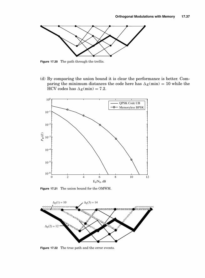
Orthogonal Modulations with Memory 17.37
Figure 17.20 The path through the trellis.
(d) By comparing the union bound it is clear the performance is better. Com-paring the minimum distances the code here has �E (min) = 10 while theHCV codes has �E (min) = 7.2.
0 2 4 6 8 10 1210–6
10–5
10–4
10–3
10–2
10–1
100
Eb/N0, dB
PW
(E)
QPSK Code UBMemoryless BPSK
Figure 17.21 The union bound for the OMWM.
∆E(3) = 14∆E(1) = 10
∆E(2) = 12
Figure 17.22 The true path and the error events.

17.38 Chapter Seventeen
TABLE 17.8 The tabulated Euclidean distance for the QPSK OMWM
�E (i, j )
�I = i
�I = j 0 1 2 3 4 5 6 7 8 9 10 11 12 13 14 15
0 0 10 10 12 10 12 12 14 10 20 12 14 12 14 14 161 10 0 12 10 12 10 14 12 20 10 14 12 14 12 16 142 10 12 0 10 12 14 10 12 12 14 10 20 14 16 12 143 12 10 10 0 14 12 12 10 14 12 20 10 16 14 14 124 10 12 12 14 0 10 10 12 12 14 14 16 10 20 12 145 12 10 14 12 10 0 12 10 14 12 16 14 20 10 14 126 12 14 10 12 10 12 0 10 14 16 12 14 12 14 10 207 14 12 12 10 12 10 10 0 16 14 14 12 14 12 20 108 10 20 12 14 12 14 14 16 0 10 10 12 10 12 12 149 20 10 14 12 14 12 16 14 10 0 12 10 12 10 14 1210 12 14 10 20 14 16 12 14 10 12 0 10 12 14 10 1211 14 12 20 10 16 14 14 12 12 10 10 0 14 12 12 1012 12 14 14 16 10 20 12 14 10 12 12 14 0 10 10 1213 14 12 16 14 20 10 14 12 12 10 14 12 10 0 12 1014 14 16 12 14 12 14 10 20 12 14 10 12 10 12 0 1015 16 14 14 12 14 12 20 10 14 12 12 10 12 10 10 0
17.8 Miniprojects
Goal: To give exposure
■ to a small scope engineering design problem in communications.■ to the dynamics of working with a team.■ to the importance of engineering communication skills (in this case oral pre-
sentations).
Presentation: The forum will be similar to a design review at a company(only much shorter). The presentation will be of 5 minutes in length with anoverview of the given problem and solution. The presentation will be followedby questions from the audience (your classmates and the professor). Each teammember should be prepared to give the presentation.
17.8.1 Project 1
Project Goals: Build a practical orthogonal modulation with memory.Convolutional codes are used in many practical applications. For example, a
block diagram of a convolutional code that is used in wireless LAN applicationsand in deep space communications is shown in Figure 17.23. The summationoperation is performed modulo-2 and the orthogonal modulation symbols aregiven as Dz(2(m − 1) + 1) = (−1)J1(m) and Dz(2(m − 1) + 2) = (−1)J2(m) .

Orthogonal Modulations with Memory 17.39
z–1 z–1 z–1 z–1 z–1 z–1I(m)
J2(m)
J1(m)
Σ
Σ
Figure 17.23 A powerful convolutional code.
(a) Characterize the OMWM by identifying the states of this modulation attime m, σ (m) and how it relates to the sequence I (m). Hint: There are 64states.
(b) Enumerate the state transitions, g1(σ (m), I (m)) for states σ (m) = 1, . . . , 8.
(c) Assume the modulation starts in σ (1) = 1 and ends in σ (Nt + 1) = 1 whereNt is the number of trellis transitions in the frame and write software thatis capable of generating the OMWM output for Kb = 100. A test sequenceof 100 bits will be sent to the class via e-mail.
(d) Provide an estimate of the minimum Euclidean squared distance of thisOMWM.

This page intentionally left blank

Appendix
AUseful Formulas
Trigonometric Identities
exp ( j θ ) = cos(θ) + j sin(θ)
cos(θ ) = 12
[exp[ j θ ] + exp[− j θ]]
sin(θ ) = 12 j
[exp[ j θ ] − exp[− j θ ]]
sin(a ± b) = sin(a) cos(b) ± cos(a) sin(b)
cos(a ± b) = cos(a) cos(b) ∓ sin(a) sin(b)
cos(a) cos(b) = 12
[cos(a − b) + cos(a + b)]
sin(a) sin(b) = 12
[cos(a − b) − cos(a + b)]
sin(a) cos(b) = 12
[sin(a − b) + sin(a + b)]
Transcendental Functions
erf (x) = 2√π
∫ x
0exp(−t2)dt
A.1
Copyright © 2007 by The McGraw-Hill Companies. Click here for terms of use.
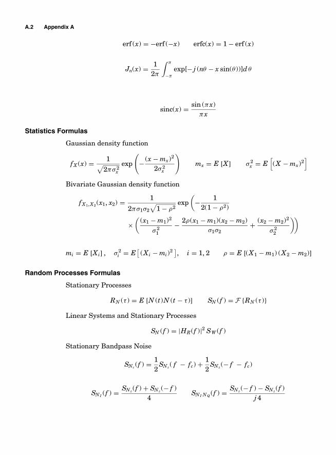
A.2 Appendix A
erf (x) = −erf (−x) erfc(x) = 1 − erf (x)
Jn(x) = 12π
∫ π
−π
exp[− j (nθ − x sin(θ ))]d θ
sinc(x) = sin (πx)πx
Statistics Formulas
Gaussian density function
fX (x) = 1√2πσ 2
x
exp
(− (x − mx)2
2σ 2x
)mx = E [X ] σ 2
x = E[(X − mx)2
]
Bivariate Gaussian density function
fX1,X2 (x1, x2) = 1
2πσ1σ2√
1 − ρ2exp(
− 12(1 − ρ2)
×(
(x1 − m1)2
σ 21
− 2ρ(x1 − m1)(x2 − m2)σ1σ2
+ (x2 − m2)2
σ 22
))
mi = E [Xi] , σ 2i = E
[(Xi − mi)2 ], i = 1, 2 ρ = E [(X1 − m1) (X2 − m2)]
Random Processes Formulas
Stationary Processes
RN (τ ) = E [N (t)N (t − τ )] SN (f ) = F {RN (τ )}
Linear Systems and Stationary Processes
SN (f ) = |HR(f )|2 SW (f )
Stationary Bandpass Noise
SNc (f ) = 12
SNz( f − fc) + 12
SNz(− f − fc)
SN I (f ) = SNz(f ) + SNz(− f )4
SN I N Q (f ) = SNz(− f ) − SNz(f )j 4

Useful Formulas A.3
Fourier Transforms
TABLE 1.1 Fourier transform table
Time Function Transform
exp[
2T 1
N0
] i=1><
i=0exp[
2T 0
N0
]X (f ) = T sin(π f T )
π f T
x(t) ={
1 − |t|T − T ≤ t ≤ T
0 elsewhereX (f ) = T
(sin(π f T )
π f T
)2
x(t) = 2W sin(2πWt)2πWt X (f ) =
{1 − W ≤ f ≤ W
0 elsewhere
x(t) ={
exp (−at) t ≤ 0
0 elsewhereX (f ) = 1
j 2π f + a
x(t) = Aexp(
j 2π f0t)
X (f ) = Aδ( f − f0)
−0.5
0
0.5
1
0 1 2 3 4 5 6 7 8
J0(x)
J1(x)J2(x)
J4(x) J6(x)
β
Figure 1.1 A plot of the low order Bessel functions of the first kind, Jn(β) versus β.

This page intentionally left blank

Appendix
BNotation
Signals and Systems
x(t) = A signal (•) = Real part of a complex signal� (•) = Imaginary part of a complex signal
xn = Fourier series coefficients of a periodic x(t)X (f ) = The Fourier transform of x(t)F (•) = The Fourier transform operator
Px = The power of x(t)Ex = The energy of x(t)
Vx(τ ) = The correlation function of x(t)Gx(f ) = The energy spectrum of x(t)
h(t) = A filter impulse responseTm = Measurement time interval
Sx( f , Tm) = A sampled power spectral densityL (•) = The Laplace transform operatorH (f ) = A filter transfer function
Random Variables
P [A] = Probability of event AFX (x) = Cumulative distribution function of a random variable Xf X (x) = Probability density function of a random variable X
σx = Standard deviation of a random variable XmX = Mean of a random variable X
E [•] = Expected valueρXY = Correlation coefficient between random variable X and random
variable Yerf(•) = Erfc function
erfc(•) = Complimentaty erfc function
B.1
Copyright © 2007 by The McGraw-Hill Companies. Click here for terms of use.

B.2 Appendix B
Bandpass Signals
xc(t) = Bandpass signalxI (t) = In-phase signalxQ(t) = Quadrature signalxz(t) = Complex envelope signalxA(t) = Amplitude signalxP (t) = Phase signal
BT = Transmission bandwidthfc = Carrier frequency
Analog Modulations
m(t) = Analog message signalW = Message signal bandwidthτp = Propagation time delayLp = Propagation lossφp = Propagation phase shift
ET = Transmission efficiencyEB = Bandwidth efficiencyAc = Transmission amplitudea = Modulation coefficient
fi(t) = Instantaneous frequencyfd (t) = Instantaneous frequency deviation
kp = Phase deviation constantkf = Frequency deviation constant (radians/s/V)fk = Frequency deviation constant (Hz/V)f p = Peak frequency deviationD = Bandwidth expansion factor
EM = Multiplexing efficiency
Random Processes
RN (τ ) , RN (t1, t2) = Correlation function of the random process N (t)ρN (τ ) , ρN (t1, t2) = Correlation coefficient of the process N (t)
SN (f ) = Power spectrum of N (t)W (t) = White noise
N0 = White noise power spectral densityBN = Noise equivalent bandwidth
Nz(t) = Complex envelope of a bandpass noiseNz(t) = Derotated complex envelopeSNRb = Baseband maximum SNRSNRo = Demodulator output SNR

Notation B.3
Digital Communications Basics
C = Channel capacityEb = Energy per bitT = Symbol time
Wb = Bit rateTp = Transmission duration
Dxz(f ) = Average energy spectrum per bitηB = Spectral efficiency (bits/s/Hz)
�I , I = Information bits�I , I = Information bit estimates
T i = Maximum likelihood metric for �I = iT i| j = Maximum likelihood metric for �I = i when the actual
transmitted signal is �I = j�E (α, β) = Square Euclidean distance between xα(t) and xβ(t){
Ad (k), �E (k)} = Squared Euclidean distance spectrum of a modulation
Kb = Number of bits to be transmitted per frameπi = A prior probability of �I = i
Linear Modulations
u(t) = Modulation pulse shapeDi(k) = Modulation symbol
a(•) = Constellation mapping, i.e., di = a(i), i = 0, M − 1�d = The constellation for a linear modulationQ = Output of filter matched to u(t)
Orthogonal Modulations
I (l) = Information bit to be transmitted at step lDz(l) = Modulation symbol for orthogonal modulationsl(t) = The spreading waveform for the lth bit for an orthogonal
modulationur (t) = The rectangular pulse
Tu = Pulse shape duration for stream modulationQ(k) = The output for the matched filter to the kth spreading for an
orthogonal modulation
Orthogonal Modulations with Memory
σ (l) = Modulation state at time lNs = Number of states in a OMWM
J (l) = Constellation label sequence, i.e., Dz(l) = a(J (l))Ms = Number of points in the constellation, i.e., J (l) = i, i = 0, Ms − 1
g1(•, •) = The modulation finite state machine, i.e., σ (l + 1) = g1(I (l), σ (l)
)

B.4 Appendix B
g2(•, •) = The output symbol selector mapping, i.e., J (l) = g2(I (l), σ (l)
)�I (l), I (l) = Information bits to be transmitted at symbol time l
Nf = Number of symbols transmittedKm = Number of bits per trellis transitionMi = Number of branches per trellis transition, i.e., Mi = 2Ks
Nm = Number of output symbols per trellis transitionR = Number of bits transmitted per symbol, i.e., R = Km/Nm

Appendix
CAcronyms
Signals and Systems
ADC = Analog to digital converterBPF = Bandpass filter
DC = Direct current, often refers to zero frequencyDTFT = Discrete time Fourier transform
I = In-phaseLPF = Lowpass filterLTI = Linear Time Invariant
Q = QuadratureSNR = Signal to noise ratio
Random Variables and Processes
AWGN = Additive white Gaussian noiseCDF = Cumulative distribution functionChF = Characteristic functionCLT = Central limit theoremPDF = Probability density functionPMF = Probability mass functionPSD = Power spectral density
RV = Random variableWSS = Wide sense stationary
Analog Communication
AM = Amplitude modulationDSB-AM = Double sideband AM
FDM = Frequency division multiplexingFM = Frequency modulation
C.1
Copyright © 2007 by The McGraw-Hill Companies. Click here for terms of use.

C.2 Appendix C
LC-AM = Large carrier AMMCPR = Message–to–Carrier Power RatioPAPR = Peak–to–Average Power Ratio
PLL = Phase–locked loopPM = Phase modulation
QCM = Quadrature carrier multiplexingSSB-AM = Single sideband AM
TV = TelevisionVCO = Voltage controlled oscillator
VSB-AM = Vestigial sideband AM
Digital Communication
AMI = Alternate mark inversionAPP = A posteriori probability
BCJR = Bahl, Cocke, Jelinek, and Raviv—an algorithm named after theinventors
BEP = Bit error probabilityBFSK = Binary frequency shift keyingBPSK = Binary phase shift keyingDTMF = Discrete tone multiple frequency
EVM = Error vector magnitudeGSM = Global system for mobile communicationsIEEE = Institute of electrical and electronic engineers
ISI = Intersymbol interferenceMAP = Maximum a posteriori
MAPBD = Maximum a posteriori bit demodulationMLBD = Maximum likelihood bit demodulationMLWD = Maximum likelihood word demodulationMFSK = M-ary frequency shift keyingMPSK = M-ary phase shift keying
MSK = Minimum shift keyingOCDM = Orthogonal code division multiplexingOFDM = Orthogonal frequency division multiplexing
OMWM = Orthogonal modulation with memoryPPM = Pulse position modulation
PWM = Pulse width modulationPWEP = Pairwise error probabilityQPSK = Quadri-phase shift keying
RLL = Run length limitedVPSK = Variable phase shift keying

Appendix
DFourier Transforms: f versus ω
This course and communications engineers in general use the variable f asopposed to ω = 2π f when examining the frequency domain representations ofsignals and systems. The reason is that units of Hertz have more of an intu-itive feel than the units of radians per second. Often undergraduate courses insignals and systems develop the theory with the notation ω. This appendix isprovided to show the differences in the results that arise from these two viewsof frequency domain analysis. First we shall define the Fourier transform forthe two variables
X (f ) =∞∫
−∞x(t)e− j 2π f tdt = F {x(t)} X (ω) =
∞∫−∞
x(t)e− j ωtdt (4.1)
The inverse Fourier transform is given as
x(t) =∞∫
−∞X (f )e j 2π f tdf = F−1 {X (f )} x(t) = 1
2π
∞∫−∞
X (ω)e j ωtdω (4.2)
The other convenient thing about working with the variable f is that theterm (2π )−1 does not need to be included in the inverse transform. A list ofFourier transform properties of different mathematical operations are listed inTable 4.1. Additionally Fourier transforms of some commonly used signals arelisted in Table 4.2.
D.1
Copyright © 2007 by The McGraw-Hill Companies. Click here for terms of use.

D.2 Appendix D
TABLE 4.1 Fourier transforms for some common mathematical operations
Operation Time Function, x(t) Transform, X (f ) Transform, X (ω)
Reversal x(−t) X (− f ) X (−ω)
Symmetry X (t) x(− f ) 2πx(−ω)
Scaling x(at) 1|a| X(
fa
)1|a| X(
ωa
)Time Delay x(t − t0) X (f )e− j 2π f t0 X (ω)e− j ωt0
Time Differentiation d n
dt n x(t) ( j 2π f )nX (f ) ( j ω)nX (ω)
Energy Ex =∞∫
−∞|x(t)|2dt Ex =
∞∫−∞
|X (f )|2dt Ex = 12π
∞∫−∞
|X (ω)|2dt
Frequency Translation x(t)e j 2π fct = x(t)e j ωct X ( f − fc) X (ω − ωc)
Convolution x(t) ∗ h(t) X (f )H (f ) X (ω)H (ω)
Multiplication x(t)y(t) X (f ) ∗ Y (f ) 12π
X (ω) ∗ Y (ω)
TABLE 4.2 Fourier transforms for some common signals
Time Function, x(t) Transform, X (f ) Transform, X (ω)
x(t) ={
1 − Tp/2 ≤ t ≤ Tp/2
0 elsewhereTp
sin(π f Tp)π f Tp
T sin(ωTp/2)ωTp/2
x(t) ={
exp (−at) 0 ≤ t
0 elsewhere1
j 2π f + a1
j ω + a
x(t) = A Aδ(f ) 2π Aδ(ω)
x(t) = Ae j ω0t = Ae j 2π f 0t Aδ( f − f 0) 2π Aδ(ω − ω0)

Appendix
EFurther Reading and
Bibliography
[Ae72] M. Abramowitz and I. E. Stegun (eds). Handbook of Mathematical Functions. U. S.Department of Commerce, Washington, DC, 1972.
[Agi00] Engineers of Agilent. Using error vector magnitude measurements to analyze and trou-bleshoot vector-modulated signals. Agilent product note 89400-14, Agilent Technologies,2000.
[Ala98] S. M. Alamouti. A simple transmit diversity technique for wireless communications.IEEE Trans. on Select Areas in Comm., 16(8):1451–1458, October 1998.
[Arm35] Edwin A. Armstrong. A method of reducing disturbances in radio signaling by a systemof frequency modulation. In IRE Conference, New York, November 1935.
[BB99] S. Benedetto and E. Biglieri. Principles of Digital Transmission. Klewer Academic Press,New York, 1999.
[BDMS91] E. Biglieri, D. Divaslar, P. J. McLane, and M. K. Simon. Introduction to Trellis-CodedModulations with Applications. Macmillan, New York, 1991.
[Bed62] E. Bedrosian. The analytical signal representation of modulated waveforms. Proceed-ings of the IRE, pp. 2071–2076, October 1962.
[Big86] E. Biglieri. Ungerboeck codes do not shape the signal power spectrum. IEEE Info. The-ory, IT-32:595–596, July 1986.
[Bra95] John Bray. The Communications Miracle. Plenum, New York, 1995.[Bre59] D. G. Brennan. Linear diversity combining techniques. Proceedings of the IRE, 47:1075–
1102, 1959.[Bur04] Russel W. Burns. Communications: A International History of the Formative Years.
Institute of Electrical Engineers, Herts, UK, 2004.[CAC01] K. Chugg, A. Anastasopoulos, and X. Chen. Iterative Detection. Kluwer Academic Press,
Boston, 2001.[Car22] J. R. Carson. Notes on the theory of modulation. Proc. IRE, vol. 10:57–64, February
1922.[Car23] J. R. Carson. Method and means for signaling with high frequency waves. Technical
Report Patent 1449382, U.S. Patent Office, 1923.[Car26] J. R. Carson. Electric Circuit Theory and Operational Calculus. McGraw-Hill, New York,
1926.[CF37] J. R. Carson and T. C. Fry. Variable frequency electric circuit theory with application to
the theory of frequency modulation. Bell Systems Technical Journal, vol. 16:513–540,1937.
[Cha66] R. W. Chang. Synthesis of band-limited orthogonal signal for multichannel data trans-mission. Bell Systems Technical Journal, vol. 45:1775–1796, December 1966.
E.1
Copyright © 2007 by The McGraw-Hill Companies. Click here for terms of use.

E.2 Appendix E
[CM86] G. R. Cooper and C. D. McGillem. Probabilistic Methods of Signals and SystemsAnalysis. Holt, Rinehart and Winston, New York, 1986.
[Com04] Federal Communication Commission. Telecommunication rules and regulations. Tech-nical Report Title 47 of the Code of Federal Regulations, Government Printing Office,http://wireless.fcc.gov/rules.html, 2004.
[Cos56] John P. Costas. Synchronous communications. Proceedings of the IRE, pp. 1713–1718,December 1956.
[Cou93] L. W. Couch. Digital and Analog Communication Systems. Macmillan, New York, 1993.[Cra91] J. W. Craig. A new simple and exact result for caluclating the probability of error for
two dimensional signal constellations. In IEEE Military Communication Conference,pp. 571–575, November 1991.
[CT92] T. M. Cover and J. A. Thomas. Elements of Information Theory. Wiley Interscience, NewYork, 1992.
[Dev00] Jay L. Devore. Probability and Statistics for Engineering and the Sciences 5. Duxbury,511 Forest Lodge Rd., Pacific Grove, CA 93950, 2000.
[DR87] W. B. Davenport and W. L. Root. An Introduction to the Theory of Random Signals andNoise. IEEE Press, New York, 1987.
[FGL+84] G. D. Forney, R. G. Gallager, G. R. Lang, F. M. Longstaff, and S. U. Qureshi. Efficientmodulation for band-limited channels. IEEE JSAC, vol. SAC-2:632–647, 1984.
[For91] G. D. Forney. Geometrically uniform codes. IEEE Info. Theory, 37:1241–1960, September1991.
[Gal01] R. Gallagher. Discrete Stochastic Processes. Klewer, 2001.[Gra53] F. Gray. Pulse code communications. Technical Report Patent 2632058, U.S. Patent
Office, 1953.[Har28] R. V. L. Hartley. Transmission of information. Bell Systems Technical Journal, p. 535,
July 1928.[Haw05] Stephen Hawking. God Created the Integers. Running Press, Philadelphia, PA, 2005.[Hay83] S. Haykin. Communications Systems. John Wiley and Sons, New York, 1983.[HCV93] P. Ho, J. Cavers, and J. Varaldi. The effect of constellation density on trellis coded
modulation in fading channels. IEEE Trans. Veh. Technol., vol. VT-42:318–325, 1993.[Hel91] C. W. Helstrom. Probability and Stochastic Processes for Engineers. Macmillan, New
York, 1991.[Huu03] Anton A. Huurdeman. The Worldwide History of Telecommunications. Wiley-
Interscience, Hoboken, NJ, 2003.[Jak74] W. C. Jakes. Microwave Mobile Communications. Wiley, New York, 1974.[Joh28] J. B. Johnson. Thermal agitation of electricity in conductors. Physical Review, vol. 32:97–
109, July 1928.[KH97] E. W. Kamen and B. S. Heck. Fundamentals of Signals and Systems Using Matlab.
Prentice-Hall, Englewood Cliffs, NJ, 1997.[Kot60] V. A. Kotel’nikov. Theory of Optimum Noise Immunity. McGraw-Hill Book Company,
New York, 1960.[KR04] James F. Kurose and Keith W. Ross. Computer Networking: A Top-Down Approach
Featuring the Internet. Addison Wesley, 2004.[Kur76] Carl F. Kurth. Generation of single-sideband signals in multiplex communication
systems. IEEE Trans. on Circuits and Systems, CAS-23:1–17, January 1976.[LC04] S. Lin and D. Costello. Error Control Coding. Prentice-Hall, Englewood Cliffs, NJ, 2004.[Lee82] W. C. Y. Lee. Mobile Communications Engineering. McGraw-Hill, New York, 1982.[Leh86] E. L. Lehmann. Testing Statistical Hypothesis. Wiley Interscience, New York, 1986.[Les69] Lawrence Lessing. Man of High Fidelity. Bantam, New York, 1969.[LG89] A. Leon-Garcia. Probability and Random Processes for Electrical Enginering. Addison-
Wesley, New York, 1989.[LGW00] A Leon-Garcia and I. Widjaja. Communication Networks. McGraw-Hill, Boston, 2000.[May84] Robert J. Mayhan. Discrete-Time and Continuous-Time Linear Systems. Addison-
Wesley, New York, 1984.[Mil63] A. Miller. Transmission system. Technical report, U.S. Patent Office, Patent 3,108,261,
1963.[Mit98] S. K. Mitra. Digital Signal Processing. McGraw-Hill, 1998.[MO98] S. Miller and R. O’Dea. Peak power and bandwidth efficient linear modulation. IEEE
Trans. Commun., 46:1639–1648, December 1998.

Further Reading and Bibliography E.3
[Nor43] D. O. North. Analysis of factors which determine signal-noise discrimination in pulsedcarrier systems. Technical Report PTR-6C, RCA Technical Report, June 1943. Reprintedin Proc. IEEE pp. 1015–1027, July 1963.
[Nyq28a] H. Nyquist. Certan topics in telegraph transmission theory. AIEE Transactions, vol.47:617–644, 1928.
[Nyq28b] H. Nyquist. Thermal agitation of lectric charge in conductors. Physical Review, vol.32:110–113, July 1928.
[OS99] A. V. Oppenheim and R. W. Schafer. Digital Signal Processing. Prentice-Hall, EnglewoodCliffs, NJ, 1999.
[Osw56] A. A. Oswald. Early history of single side band. Proc. of IRE, vol. 44:1676–1679, Decem-ber 1956.
[OW97] A. V. Oppenheim and A. S. Willsky. Signals and Systems. Prentice-Hall, Upper SaddleRiver, NJ, 1997.
[Pap84] A. Papoulis. Probability, Random Variables and Stochastic Processes. McGraw-Hill,New York, 1984.
[Pet89] Blake Peterson. Spectrum analysis basics. Application note 150, Hewlett Packard, 1989.[PM88] J. G. Proakis and Manolakis. Introduction to Digital Signal Processing. Macmillan,
1988.[Poo88] H. V. Poor. An Introduction to Signal Detection and Estimation. Springer-Verlag, New
York, 1988.[Por97] Boaz Porat. A Course in Digital Signal Processing. Wiley, 1997.[Pro89] J. G. Proakis. Digital Communications. McGraw-Hill, New York, 1989.[PS94] J. G. Proakis and Masoud Salehi. Communications System Engineering. Prentice-Hall,
Englewood Cliffs, NJ, 1994.[Ric45] S. O. Rice. Mathematical analysis of random noise. Bell System Technical Journal,
24:96–157, 1945.[Ric48] S. O. Rice. Statistical properties of a sine-wave plus random noise. Bell System Technical
Journal, vol. 27:109–157, 1948.[SB89] D. Saha and T. Birdsall. Quadrature-quadrature phase-shift keying. IEEE Trans. Com-
mun., COM-37:437–448, May 1989.[SBS66] M. Schwartz, W. R. Bennett, and S. Stein. Communication Systems and Techniques.
McGraw-Hill, New York, 1966.[Sha48] Claude Shannon. A mathematical theory of communication. Bell System Technical Jour-
nal, 1948.[Skl88] B. Sklar. Digital Communications. Prentice-Hall, Englewood Cliffs, NJ, 1988.[SS87] W. E. Saban and E. Schoenike. Single Sideband Systems and Circuits. McGraw-Hill,
New York, 1987.[Sti99] David Stirzaker. Probability and Random Variables: A Beginner’s Guide. Cambridge
University Press, 40 West 20th St. New York, NY 10011-4211, 1999.[SW49] Claude E. Shannon and Warren Weaver. The Mathematical Theory of Communication.
University of Illinois Press, Urbana, IL, 1949.[SW02] Henry Stark and John W. Woods. Probability and Random Processes with Applications
to Signal Processing. Prentice-Hall, Upper Saddle River, NJ, 2002.[Tan02] Andrew S. Tanenbaum. Computer Networks, Fourth Edition. Prentice-Hall, 2002.[Ung82] Gottfried Ungerboeck. Channel coding with multilevel/phase signals. IEEE Info. The-
ory, IT-28:55–67, January 1982.[VO79] A. J. Viterbi and J. K. Omura. Principles of Digital Communication and Coding.
McGraw-Hill, New York, 1979.[Wal97] H. R. Walker. VPSK and VMSK modulation transmit digital audio and video at
15 bit/s/Hz. IEEE Trans. on Broadcasting, 43:96–103, 1997.[WB00] J.C. Whitaker and K. B. Benson. Standard Handbook of Video and Television Engineer-
ing. McGraw-Hill, New York, 2000.[Web87] C. L. Weber. Elements of Detection and Signal Design. Springer Verlag, New York, 1987.
Reprint of a 1967 book.[Wes01] Douglas B. West. Introduction to Graph Theory. Prentice-Hall, 2001.[Wic95] S. B. Wicker. Error Control Systems for Digital Communications and Storage. Prentice-
Hall, Upper Saddle River, NJ, 1995.[Wie49] Norbert Wiener. The Extrapolation, Interpolation, and Smoothing of Stationary Time
Series with Engineering Applications. Wiley, New York, 1949.

E.4 Appendix E
[WJ65] J. M. Wozencraft and I. M. Jacobs. Principles of Communications Engineering. JohnWiley and Sons, New York, 1965.
[YG98] Roy D. Yates and David J. Goodman. Probability and Stochastic Processes: A FriendlyIntroduction for Electrical and Computer Engineers. Wiley, New York, 1998.
[Zie86] A. Van Der Ziel. Noise in Solid State Devices. Wiley-Interscience, New York, 1986.[ZTF89] R. E. Ziemer, W. H. Trantor, and D. R. Fannin. Signals and Systems: Continuous and
Discrete. Macmillan, New York, 1989.

Index
acronyms, listed, C.1–C.2additive white Gaussian noise (AWGN)
bandpass noise and, 10.18–10.19,10.21–10.23, 10.25–10.26
carrier frequency filtering and, 10.1complex, 10.18–10.19, 13.48, 13.2,
13.22, 14.29fidelity evaluation and, 11.1, 11.4frequency shift keying and, 14.19matched filter and, 13.22mini-project on, 9.44multiple bit transmission and, 14.28,
14.29–14.30, 14.33, 14.36optimal demodulator complexity and,
15.33–15.36, 15.37, 15.40, 15.41,15.46
random processes and, 9.35–9.36linear systems and, 9.25, 9.27,
9.30–9.31, 9.32–9.34, 9.39thermal noise and, 9.20–9.21
satellite communication and, 16.21single bit demodulation and, 13.2,
13.40, 13.41, 13.42–13.47, 13.48spectral efficiency and, 12.9telephone communication and, 12.14
adjacent channel interference (ACI),10.26
affine modulation, 6.8–6.12demodulation and, 6.13–6.16modulator for, 6.12–6.13
Agilent 89600, 4.8Alternate Mark Inversion (AMI)
modulation, 17.9–17.11, 17.13,17.15, 17.33, 17.34
amplitude, 4.3, 10.4amplitude modulation (AM), 6.1
See also under homework problemsaffine modulation and, 6.8–6.12
demodulation and, 6.13–6.16modulator for, 6.12–6.13
bandpass signals and, 5.6
bandwidth and, 5.10defined, 1.8disadvantages of, 7.1–7.2example solutions for, 6.42–6.44linear modulation and, 6.1, 6.3–6.8mini-projects on, 6.44–6.46quadrature modulation and, 6.16–6.17,
6.27demodulation and, 6.23–6.27modulator for, 6.22–6.23SSB-AM and, 6.19–6.21VSB filter design and, 6.17–6.19
signal to noise ratio and, 11.20, 11.24transformation of random variables
and, 3.19–3.20analog communication, 5.1
See also amplitude modulation (AM);angle modulation; fidelity inanalog demodulation
acronyms for, C.1–C.2example solutions for, 5.15–5.17history of communication and, 1.1homework problems on, 5.12–5.15message signal characterization and,
5.1–5.4multiplexing signals and, 8.8–8.13notation for, B.2performance metrics for, 5.8–5.11phase-locked loop and, 8.1–8.4technique comparison and, 7.24–7.25text overview and, 1.8–1.9transmission and, 5.5–5.8
analog-to-digital conversion (ADC), 2.23,4.23
angle modulation, 7.1See also under homework problemsAM disadvantages and, 7.1–7.2bandpass signal and, 7.2–7.6bandwidth of, 7.12–7.14, 7.15–7.17complexity and, 7.24, 11.19defined, 1.8
I.1
Copyright © 2007 by The McGraw-Hill Companies. Click here for terms of use.

I.2 Index
angle modulation (Cont.):demodulation and, 7.19–7.24
signal to noise ratio and, 11.12–11.17derotated noise and, 11.21example solutions for, 7.37–7.39introduction of, 7.2mini-projects on, 7.39–7.40modulators for, 7.6–7.7narrowband, 7.14, 7.18–7.19phase-locked loop and, 8.4–8.8signal to noise ratio and, 11.12–11.17,
11.20sinusoidal message signal and, 7.7–7.14spectral efficiency and, 11.19
antipodal signaling, 13.28aperiodic signals, 2.4–2.5a posteriori probability (APP), 13.5, 13.7,
14.31a priori probability, 13.49Armstrong, Edwin H., 7.2Arnold, H. D., 6.23
bandpass demodulation, 11.4–11.6bandpass noise, 10.19
amplitude of, 10.4complex AWGN and, 10.18–10.19complex envelope and, 10.6–10.12correlation function of, 10.6, 10.10,
10.17defined, 10.1example solutions for, 10.27–10.29homework problems on, 10.19–10.27lowpass noise and, 10.3mini-projects on, 10.29–10.30multiple bit transmission and, 14.28performance analysis and, 10.2–10.3phase of, 10.4random processes and, 10.4–10.6signal to noise ratio and, 11.20solution of canonical problem and,
10.15–10.17spectral characteristics of, 10.2, 10.3,
10.12–10.15bandpass signals, 4.18
See also under homework problemsaffine modulation and, 6.14amplitude modulation and, 1.8angle modulation and, 1.8, 7.2–7.6,
7.37
bandwidth of, 4.13baseband representation of, 4.2–4.6complex envelope and, 4.9defined, 4.2direct digital synthesis and, 7.6DSB-AM and, 6.28, 6.31example solutions for, 4.30–4.33linear systems and, 4.14–4.17, 6.1mini-projects on, 4.33–4.34notation for, B.2text overview and, 1.8vector diagram of, 4.8–4.9VSB-AM signals and, 6.17, 6.18
bandwidthAM disadvantages and, 7.1analog communication and, 5.2–5.3,
6.1, 6.3of angle modulation, 7.12–7.14,
7.15–7.17, 7.24, 7.25–7.27, 7.30,7.33
of bandpass signals, 4.2, 4.13, 4.26complexity and, 11.19energy spectrum and, 13.29FM demodulation and, 8.14frequency domains and, 2.14–2.16of frequency shift keying, 13.35, 14.21homework problems on, 2.27, 2.31limiting, 5.13linear modulations and, 6.1, 6.3, 15.11mini-project on, 2.36–2.37modems and, 12.11OFDM and, 15.21–15.22, 16.6performance and, 14.19, 14.20of periodic signals, 2.17of phase shift keying, 14.26sampling and, 2.23–2.24signal to noise ratio and, 11.20spectral efficiency and, 12.4, 12.6–12.7,
12.9–12.10spectral mask and, 16.1squared cosine pulse and, 16.3–16.4,
16.19transmission efficiency and, 5.10
baseband data communications, 12.2baseband processing power, 1.6Baud rate, 15.27Bayes theorem, 3.4–3.5, 3.15–3.16,
3.25–3.26, 3.33, 13.7, 13.8, 14.4,14.31

Index I.3
Bessel function, 7.10–7.11, 7.12, 7.30binary data communications, 12.1binary frequency shift keying (BFSK),
13.30–13.36, 13.39, 13.41, 13.47,13.52
binary phase shift keying (BPSK)eye diagram and, 16.20orthogonal modulation and,
15.37–15.38OCDM, 15.22, 15.24, 15.25OFDM, 15.18–15.19, 15.38OMWM, 17.21, 17.32, 17.33, 17.34,
17.35–17.36single bit demodulation and,
13.36–13.39, 13.42, 13.47, 13.52stream modulation and, 15.27, 15.28,
16.24–16.26binary symmetric channel, 3.5bit error probability (BEP)
a priori probability and, 13.17AWGN and, 13.41, 13.45–13.46fidelity and, 13.14filter design and, 13.6, 13.18, 13.20frequency shift keying and,
13.32–13.33, 13.35–13.36, 13.41multiple bit transmission and,
14.32phase shift keying and, 13.38, 13.42signal design and, 13.26–13.28single bit demodulation and, 13.42,
13.48Boltzmann’s constant, 9.19
carrier frequency assignments, 4.2carrier modulated communications, 4.14,
12.2Carson, J. R., 6.4–6.5, 6.23, 7.2, 7.15Carson’s rule, 7.15–7.16, 7.27, 7.28, 7.31,
7.33, 7.34, 7.35, 7.37–7.39Cavers, J., 17.5, 17.30, 17.33central limit theorem (CLT), 3.10, 3.21circuit theory, 1.3coherent amplitude demodulation,
11.6–11.12coherent demodulation, 5.8, 6.6–6.8, 6.23,
11.5–11.9, 11.19color patterns, 4.19–4.20communication engineering. See specific
subject matter
communication systems, modern, 1.4–1.6.See also analog communication;digital communication
communication theoryby Bayes, 3.4–3.5, 3.15–3.16, 3.25–3.26,
3.33, 13.7, 13.8, 14.4, 14.31central limit, 3.10, 3.21circuit, 1.3convolution, 2.10, 2.19decision, 13.1detection, 14.2, 14.4, 14.31duality theorem, 2.10on Fourier transform, 2.10–2.14frequency translation, 2.11, 4.10–4.11historical perspective on, 1.1–1.3information, 1.7, 12.8–12.10, 13.39,
14.26, 14.27, 17.2Markov chains, 17.14by Parseval, 2.8–2.10, 2.12, 5.17, 6.44,
7.11, 9.24practice and, 1.6, 9.25probability, 1.8, 3.2by Rayleigh, 2.10, 2.12, 4.14, 13.26,
13.50statistical hypothesis testing and,
13.3–13.6text focus and, 1.3, 1.6–1.7total probability, 3.4, 3.15translation and dilation, 2.11Wiener-Khinchin, 9.17–9.18
complement, 3.2complex baseband representation, 4.1,
4.18of bandpass signal, 4.2–4.6carrier modulated signals and, 4.14complex envelope and, 4.9–4.13linear systems and, 4.14–4.17
complex envelopeanalog modulation and, 5.6, 6.9–6.10,
7.1angle modulation and, 7.1, 7.3, 7.8,
7.12, 7.19–7.20, 7.30, 7.36bandpass filters and, 4.25–4.26bandpass noise and, 10.6–10.12,
10.20–10.21, 10.23of bandpass random process, 10.4–10.6bandpass signals and, 4.4, 4.6,
4.23–4.24, 4.26–4.27digital transmission and, 12.2

I.4 Index
complex envelope (Cont.):DSB-AM signal and, 6.5linear analog modulation and, 6.1multiple bit transmission and, 14.28notation for, B.2sampling rate and, 4.23signal to noise ratio and, 11.10,
11.20–11.21spectral characteristics of, 4.9–4.13text overview and, 1.8visualization of, 4.6–4.9VSB-AM and, 6.17, 6.23
complexitySee also optimal demodulator
complexityanalog performance metrics and, 5.9angle modulation and, 7.24, 11.19digital communication and, 1.10, 12.4,
12.5frequency shift keying and, 13.39,
14.21, 14.36of modems, 12.10–12.11multiplexing and, 8.13noncoherent demodulation and, 11.11of orthogonal modulations, 16.11, 17.1,
17.2OFDM, 16.6OMWM, 17.2, 17.4, 17.8, 17, 11,
17.28phase shift keying and, 14.23, 14.26stream modulation and, 16.21text overview and, 1.3, 1.8, 1.10VSB-AM, 6.24
complex signals, 2.5conditional probability, 3.3, 3.33–3.34constellation mapping, 15.2, 15.36, 17.4,
17.17, B.3continuous random variable, 3.6continuous time signals, 2.6, 2.23–2.24convolutional codes, 17.21–17.23convolution theorem, 2.10, 2.19Costas loop, 6.7–6.8, 6.28, 8.1, 8.2Craig, J. W., 15.38cumulative distribution function (CDF)
defined, 3.6–3.7finding, 3.12joint, 3.14properties of, 3.7–3.8
random processes and, 9.4random variables and, 3.11, 3.19–3.20
cyclostationary random process,17.18–17.19
decibel notation, 2.14decision theory, 13.1deep space communication, 1.1–1.2, 4.2,
12.10, 12.13–12.14, 16.21detection theory, 14.2, 14.4, 14.31deterministic signals, 2.1–2.6. See also
complex baseband representationdevices engineer, 1.2differentiator, 2.22digital communication, 12.2
See also multiple bit transmission;single bit demodulation structures
acronyms for, C.2coherent, 13.2–13.3demodulation and, 12.3–12.4example solutions for, 12.14performance and, 12.4–12.5homework problems on, 12.11–12.14mini-projects on, 12.14–12.15modulation and, 12.2–12.3notation for, B.3performance and, 12.4, 12.7–12.8
bandwidth efficiency and, 12.6–12.7complexity and, 12.5fidelity and, 12.4–12.5limits on, 12.8–12.10
spectral efficiency ofcontainment and, 16.1–16.2linear stream modulations and,
16.7–16.11orthogonal modulations and,
16.5–16.7, 16.11–16.18squared cosine pulse and, 16.3–16.5
statistical hypothesis testing and,13.3–13.5
text overview and, 1.10digital oscilloscope, 1.7digital revolution, 1.1digital signal processors, 2.6Dirac delta function, 3.8direct digital synthesis (DDS), 7.6discrete Fourier transform (DFT), 2.23,
2.25

Index I.5
discrete random variables, 3.6, 3.8discrete time Fourier transform (DTFT),
2.23, 2.24discrete time signals, 2.6, 2.23discriminator, 7.22–7.23Doppler effect, 4.24double sideband-amplitude modulation
(DSB-AM)angle modulation and, 7.9, 7.24,
7.33–7.34bandpass noise and, 10.24–10.25, 10.30complexity and, 11.19demodulation and, 6.5–6.8, 8.2example solutions on, 6.42–6.43high fidelity broadcasting and, 8.15homework problems on, 6.27–6.28,
6.35–6.36, 6.39, 6.41–6.42invention of, 6.4mini-project on, 6.45modulator for, 6.5multiplexing and, 8.14phase detector and, 8.3power of, 6.3quadrature modulation and, 6.16signal to noise ratio and, 11.6–11.8,
11.20, 11.22, 11.23, 11.26single bit demodulation and, 13.47spectral efficiency and, 11.19
duality theorem, 2.10dual tone multiple frequency (DTMF),
12.11–12.12, 14.32
Einstein, Albert, 1.6electronic test equipment, 2.13–2.14embedded computer, 1.2energy signals, 2.1–2.4energy spectrum
affine modulation and, 6.11–6.12angle modulation and, 7.9of bandpass signal, 4.2, 4.3, 4.8, 4.13bandwidth and, 2.31of complex envelope, 4.9–4.10, 4.11,
4.12defined, 2.11–2.12frequency shift keying and, 14.20LCM-AM and, 6.32linear modulations and, 2.19, 6.1, 15.10of lowpass signals, 2.15
message signal characterization and,5.1–5.2, 5.3
notation for, B.1of OCDM, 15.25–15.26of OFDM, 15.19–15.22of OMWM, 17.9–17.15, 17.17–17.21periodic pulse and, 2.17–2.18rectangular pulse and, 2.15sinc pulse and, 2.16single bit demodulation and, 13.29spectral density and, 9.16of SSB-AM signal, 6.21of stream modulation, 15.29–15.30of VSB-AM signal, 6.18–6.19
Englund, Carl, 6.4erf function, 3.11, 13.15–13.16error vector magnitude (EVM),
16.13–16.14, 16.27Ethernet, 15.42–15.43, 15.50Euclidean distance
defined, 13.12–13.13frequency shift keying and,
13.32–13.33, 14.40homework problems on, 15.35, 13.50linear modulation and, 15.8–15.9natural mapping and, 14.21notation for, B.3orthogonal modulations and,
15.15–15.16OMWM, 17.4–17.5, 17.7, 17.22,
17.25, 17.30, 17.31–17.32, 17.34,17.35–17.36
phase shift keying and, 13.38, 14.23signal design and, 13.26, 13.28,
13.51–13.52, 14.16union bound and, 14.11–14.15
Euler’s rule, 2.5, 2.6, 2.33example solutions
for amplitude modulation, 6.42–6.44for analog communication, 5.15–5.17for angle modulation, 7.37–7.39for bandpass noise, 10.27–10.29for bandpass signals, 4.30–4.33for digital communication, 12.14for multiple bit transmission,
14.37–14.40for multiplexing, 8.19for OMWM, 17.36–17.37

I.6 Index
example solutions (Cont.):for optimal demodulator complexity,
15.48–15.53for probability/random variables,
3.33–3.36for random processes, 9.42–9.43for signals, 2.33–2.36for signal to noise ratio, 11.26–11.28for single bit demodulation,
13.50–13.55for spectral efficiency, 16.22–16.23
eye diagram, 16.16–16.18, 16.20
Federal Communications Commission(FCC), 5.10, 5.11, 16.1, 6.30, 6.31
fidelityangle modulation and, 7.2, 7.3, 7.20,
7.24, 7.25, 7.33BFSK and, 13.33in digital communication, 12.4–12.5design problem and, 13.6FM broadcasting and, 5.10–5.11function of, 5.9, 12.4linear modulations and, 15.11of message reconstruction, 5.12, 7.24,
7.25, 10.19, 12.4, 13.14multiple bit transmission and,
14.7–14.10noise effects and, 5.12orthogonal modulations and, 15.15,
17.1See also fidelity of OMWMOCDM, 15.24–15.25, 15.26OFDM, 15.19, 15.22
performance comparison and, 5.9QPSK and, 15.8satellite communication and, 12.13single bit demodulation and, 13.6,
13.14–13.18signal characterization and, 5.1, 5.3–5.4signal design and, 13.25spectral mask and, 16.2text overview and, 1.3, 1.10
fidelity in analog demodulationangle demodulation and, 11.12–11.17bandpass demodulation and, 11.4–11.6coherent amplitude demodulation and,
11.6–11.12example solutions for, 11.26–11.28
homework problems on, 11.20–11.25mini-projects on, 11.29noncoherent demodulation and,
11.9–11.12pre-emphasis and, 11.17–11.19unmodulated signals and, 11.1–11.3
fidelity of OMWM, 17.2, 17.9AMI modulation and, 17.10–17.11convolution codes and, 17.22–17.23Euclidian distance and, 17.4–17.5example on, 17.5–17.7redundancy and, 17.3–17.4transmission rates and, 17.16trellis codes and, 17.25–17.26formulas, useful, A.1–A.3
Fourier series, 2.6–2.8analog communication and, 5.12–5.13,
5.15–5.16angle modulation and, 7.8–7.10, 7.12,
7.30bandpass signals and, 4.19, 4.31DSB-AM and, 6.27example solutions and, 2.33homework problems on, 2.26, 2.30,
2.31, 3.6, 6.35–6.36linear time-invariant system and, 2.21,
2.22mathematical representation of, 2.6–2.7properties of, 2.8
Fourier transformanalog communication and, 5.13, 5.15angle modulation and, 7.7bandpass noise and, 10.12, 10.13,
10.15bandpass signals and, 4.16–4.17bandwidth and, 2.16complex baseband representation and,
4.9, 4.10–4.11complex signals and, 2.5discrete time signals and, 2.23example solutions for, 2.35formulas for, 2.9, A.3frequency and, 9.16homework problems on, 2.26–2.27,
2.29–2.30, 2.33, 6.40linearity and, 2.19, 16.21of OFDM, 15.20of OMWM, 17.19properties of, 2.9–2.10

Index I.7
notation for, B.1of periodic signals, 2.16–2.18random processes and, 9.24, 9.32signal to noise ratio and, 11.4single bit demodulation and, 13.54squared cosine pulse and, 16.3–16.5theory and, 2.10–2.14variable f and, D.1–D.2of VSB-AM signal, 6.17
frequency division multiplexing (FDM),8.10–8.13, 8.14
frequency domainangle modulation and, 7.10bandpass signals and, 4.15–4.16, 4.26,
4.27bandwidth of signals and, 2.14–2.16,
2.17of complex envelope, 6.43example solutions and, 2.34–2.35formula for, 2.5filtering and, 2.20Fourier series and, 2.6–2.8, 2.18Fourier transform and, 2.9–2.14,
2.16–2.18, 2.35matched filter and, 13.20LC-AM and, 6.29orthogonal modulations and, 15.45of output signal, 2.25Parseval’s theorem and, 5.17random processes and, 9.24sampling and, 2.23signal analysis and, 2.6stationary noise and, 9.15–9.16text overview and, 1.8time signals and, 2.23–2.24, 2.34
frequency doubler, 2.28, 2.36frequency modulation (FM)
analog communication and, 1.9angle modulation and, 7.16
bandpass signals and, 7.4–7.6bandwidth and, 7.12–7.14example solutions for, 7.39homework problems on, 7.27, 7.28,
7.32, 7.33–7.34instantaneous frequency deviation
and, 7.3phase detector and, 7.20sinusoidal message signal and,
7.7–7.8
bandpass noise and, 10.26–10.27bandpass signals and, 5.6bandwidth and, 5.10–5.11demodulation and, 8.14differentiator and, 2.22high fidelity broadcasting and,
8.14–8.15multiplexing and, 8.12–8.13, 8.17phase-locked loop and, 8.4–8.5, 8.6phase modulation and, 11.18–11.19signal to noise ratio and, 11.15–11.19,
11.20, 11.23single bit demodulation and, 13.47voltage controlled oscillator and, 7.6
frequency shift keying, 12.12See also M-ary frequency shift keying
(MFSK)binary, 13.30–13.36, 13.39, 13.41,
13.47, 13.52Frequency Translation Theorem, 2.11,
4.10–4.11Fry, T. C., 7.15
Gaussian random processSee also additive white Gaussian noise
(AWGN)bandpass noise and, 10.3, 10.7–10.9,
10.26, 10.28–10.29defined, 9.5filter output and, 13.10linear filtering of, 9.23as model, 9.4signal to noise ratio and, 11.25stationary, 9.11–9.15, 9.16, 9.19, 9.24
Gaussian random variables, 3.10CDF of, 3.11central limit theorem and, 3.21characterization of, 9.5–9.9correlation function and, 9.12–9.15erf function and, 3.11homework problems on, 3.27, 3.28, 3.29,
3.30, 3.32, 9.38–9.39, 9.41–9.42likelihood metrics and, 14.8–14.9multiple dimensional, 3.22–3.23pairwise error probability and, 14.11PDF of, 3.10–3.11single bit demodulation and,
13.14–13.16, 13.49two, 3.16–3.19

I.8 Index
geometric uniformity, 14.16, 17.31–17.32Gray mapping, 14.21–14.22, 14.29group delay, 2.32
Hadamard matrices, 15.40–15.41Hermitian symmetric, 2.8, 2.9, 4.9–4.10high fidelity audio transmission, 5.3–5.4,
5.10–5.11, 8.14–8.15Hilbert transform, 6.20–6.21, 6.25, 6.40,
6.41, 6.43, 6.46Ho, P., 17.5, 17.30, 17.33homework problems
on amplitude modulation (AM)bandpass signal and, 6.31demodulation and, 6.31, 6.34–6.35,
6.36, 6.41DSB-AM and, 6.27–6.28, 6.35–6.36,
6.39, 6.41–6.42energy spectrum and, 6.32Fourier transform and, 6.40LC-AM and, 6.28–6.29, 6.32–6.33,
6.36, 6.37–6.38, 6.41–6.42quadrature modulation and,
6.33–6.34, 6.40radio output limitations and,
6.30–6.31SSB-AM and, 6.36, 6.38–6.39VSB-AM and, 6.32–6.33, 6.35
on analog communication, 5.12–5.15on angle modulation
bandwidth and, 7.25–7.27, 7.30, 7.33complex envelope and, 7.36demodulation and, 7.32Fourier series and, 7.30frequency modulation and, 7.27, 7.28message signals and, 7.25, 7.30phase modulation and, 7.25, 7.26,
7.27, 7.28, 7.31, 7.32–7.33,7.34–7.37
sinusoidal angle modulation and,7.25–7.26
sinusoidal message signal and,7.28–7.29, 7.30–7.31, 7.34
on bandpass noise, 10.19–10.27on bandpass signals
amplitude imbalance and, 4.29–4.30analog-digital conversion and, 4.23bandwidth and, 4.26color patterns and, 4.19–4.20
complex envelope and, 4.19,4.23–4.24, 4.25–4.27
design problem and, 4.21energy spectrum and, 4.18, 4.20Fourier series and, 4.19Fourier transforms and, 4.27–4.28frequency domain representation
and, 4.26in-phase/quadrature signals and,
4.21linear systems and, 4.24–4.25periodic signals and, 4.23radar signals and, 4.24, 4.28time delays and, 4.21
on communication theory, 1.10–1.11on digital communication, 12.11–12.14on FM demodulation, 8.14on high fidelity broadcasting, 8.14–8.15on multiple bit transmission
AWGN and, 14.29–14.30, 14.33,14.36
binary system and, 14.32dual tone multiple frequency and,
14.32–14.33frequency shift keying and,
14.28–14.29, 14.36PDF and, 14.28phase shift keying and, 14.29pulse position modulation and,
14.34–14.35union bound and, 14.32wireless local network and,
14.35–14.36word error probability and, 14.27
on multiplexing, 8.14, 8.15–8.18on OMWM, 17.30–17.36on optimal demodulator complexity
AWGN and, 15.33–15.36, 15.37,7.30–7.31, 15.41, 15.46
error probability and, 15.38–15.39frequency shift keying and, 15.46Hadamard matrices and, 15.40–15.41linear modulation and, 15.31–15.32,
15.34, 15.36–15.37, 15.41–15.42,15.44–15.45
local area networks and, 15.42–15.43orthogonal modulation and,
15.37–15.38, 15.40, 15.41, 15.45phase shift keying and, 15.47–15.48

Index I.9
quadrature amplitude modulationand, 15.31, 15.47
spectral efficiency and, 15.46stream modulation and, 15.36,
15.39–15.40, 15.41union bound and, 15.32–15.33wireless network protocol and, 15.41
on phase-locked loop, 8.13–8.14on random processes
AWGN and, 9.30–9.31, 9.32–9.34,9.35–9.36, 9.39
correlation function and, 9.37–9.38Fourier transform and, 9.32Gaussian random variables and,
9.38–9.39, 9.41–9.42Gaussian/stationary modeling and,
9.40independent white Gaussian noise
and, 9.38linear systems and, 9.32, 9.39message signals and, 9.39power spectrum and, 9.34–9.35SNR and, 9.40–9.41spectral density and, 9.31–9.32, 9.34
on random variables/probability,3.23–3.32
on signals, 2.25–2.33on signal to noise ratio, 11.20–11.25on single bit demodulation structures
AWGN and, 13.40, 13.41–13.47, 13.48frequency shift keys and, 13.41, 13.47MAPBD and, 13.41phase shift keys and, 13.42, 13.47random variables and, 13.49, 13.50
on spectral efficiency, 16.18–16.22
independent white Gaussian noise, 9.38information theory, 1.7, 12.8–12.10,
13.39, 14.26, 14.27, 17.2in-phase (I) component, 4.3, 4.6, 10.4International Organization for
Standardization (ISO), 1.4intersymbol interference (ISI)
eye diagram and, 16.16–16.17orthogonal modulations and, 15.27,
16.28scatter plot and, 16.12, 16.13stream modulation and, 15.36, 15.50,
16.8, 16.9, 16.16, 16.24–16.26
Jacobs, Irwin, 1.6Johnson, J. B., 9.19Johnson–Nyquist noise, 9.1, 9.19–9.21.
See also random processesJoules, 2.4
Laplace transform, 2.18, 8.4, 8.6, 8.7, 8.8large carrier amplitude modulation
(LC-AM)angle modulation and, 7.14, 7.18, 7.23,
7.24complex envelope and, 6.9–6.10complexity and, 11.19demodulation and, 6.13–6.16energy spectrum of, 6.9, 6.11–6.12homework problems on, 6.28–6.29,
6.32–6.33, 6.36, 6.37–6.38,6.41–6.42
MCPR of, 6.10–6.12mini-project on, 6.45modulator for, 6.12–6.13quadrature modulation and, 6.16, 6.27signal to noise ratio and, 11.9–11.10,
11.11, 11.19, 11.29spectral efficiency of, 11.19
layered architecture, 1.4–1.6Leibniz rule, 3.12–3.13, 3.19linear modulation, 15.11–15.13
advantage of, 15.31bandpass signal and, 4.25constellation plot and, 15.2–15.3error rate evaluation for, 15.6–15.9example solutions for, 15.52Fourier transform and, 2.33, 16.21homework problems on, 15.31–15.32,
15.34, 15.36–15.37, 15.41–15.42,15.44–15.45
MLWD for, 15.3–15.6mobile devices and, 12.8notation for, B.3phase-locked loop and, 8.4, 8.6–8.8quadrature amplitude and, 15.10random processes and, 9.23–9.27, 9.32,
9.39spectral characteristics of, 15.10,
16.7–16.11linear stream modulation, 16.18, 16.19linear time-invariant (LTI) system,
2.18–2.22, 13.5

I.10 Index
logic analyzer, 1.7loop filter, 8.3lowpass filter
analog fidelity and, 11.3, 11.7, 11.11,11.14, 11.16
bandpass signals and, 4.14complex envelope and, 4.6, 10.7frequency response and, 8.7Gaussian noise and, 9.11, 9.24–9.25homework problems on, 2.27, 7.36,
9.30, 9.33, 11.23, 11.25LTI filter and, 2.19Matlab and, 9.3mini-project on, 10.30random processes and, 9.29signal to noise ratio and, 11.7,
11.23–11.24single bit demodulation and, 13.7,
13.57VSB-AM demodulator and, 6.23
Markov chains theory, 17.14M-ary frequency shift keying (MFSK)
advantages of, 14.21energy spectrum of, 14.19–14.20error rate of, 14.18–14.19, 14.26homework problems on, 14.27,
14.28–14.29, 14.32, 14.36OMWM and, 17.23optimal demodulator complexity and,
15.46signal set of, 14.17–14.18union bound for, 14.19
M-ary phase shift keying (MPSK), 14.17advantages of, 14.26demodulation and, 14.22–14.23energy spectrum of, 14.25–14.26error rate of, 14.23–14.25homework problem on, 14.29linear modulation and, 15.11–15.12,
15.32OMWM and, 17.35optimal demodulator complexity and,
15.1, 15.2, 15.4signal set of, 14.21–14.22spectral efficiency and, 16.23union bound for, 14.23–24, 15.32–15.33
mathematical foundations, 1.7–1.8
Matlab, 2.2angle modulation and, 7.28, 7.39, 7.40bandpass signals and, 4.33bandwidth computation and, 2.18Bessel function and, 7.30complex baseband representation and,
4.1continuous time signals and, 2.6double sideband modulation and, 6.45eye diagram and, 16.17large carrier modulation and, 6.45optimal demodulator complexity and,
15.54–15.55probability density function and, 3.9random variables and, 3.6, 3.10, 3.12,
3.15, 3.29, 3.31sample paths and, 9.3single bit demodulation and, 13.54single sideband modulation and, 6.46statistical averages and, 9.4–9.5time variables and, 2.23–2.25unwrapping function and, 7.20
Matlab code, 5.17maximum a posteriori bit demodulation
(MAPBD), 13.7, 13.10, 13.41, 14.2maximum a posteriori word demodulator
(MAPWD), 14.4–14.5, 14.7, 14.9maximum likelihood bit demodulator
(MLBD), 13.12a priori probability and, 13.16–13.18filter design and, 13.20frequency shift keying and, 13.32geometric interpretation of,
13.12–13.13matched filter and, 13.21–13.23, 13.28multiple bit transmission and,
14.1–14.2orthogonal modulations and, 15.15,
15.18, 15.24phase shift keying and, 13.38single bit demodulation and, 13.41stream modulation and, 15.39
maximum likelihood word demodulator(MLWD), 14.5–14.6
frequency shift keying and, 14.18homework problems on, 14.27, 14.30,
14.33, 14.36, 15.35–15.36, 15.42,15.43

Index I.11
for linear modulation, 15.3–15.6, 15.31,15.32, 15.45
OMWM and, 17.4–17.5optimal demodulator complexity and,
14.7phase shift keying and, 14.22word error probability of, 14.9, 14.27
memory, 17.2. See also orthogonalmodulation with memory (OMWM)
message signal characterization, 5.1–5.4microprocessor, 1.2Miller code, 17.26–17.28minimum distance decoder, 15.4minimum shift keying (MSK), 13.34mini-projects
on bandpass noise, 10.29–10.30on bandpass signals, 4.33–4.34on digital communication, 12.14–12.15on multiple bit transmission,
14.40–14.41on multiplexing, 8.20on OMWM, 17.37–17.39on optimal demodulator complexity,
15.53–15.55on probability/random variables,
3.36–3.37on random processes, 9.44–9.45on signals, 2.36–2.37on signal to noise ratio, 11.29on single bit demodulation, 13.55–13.57on spectral efficiency, 16.23–16.28
mixed random variable, 3.6mobile devices, 12.8modems
bandpass signals and, 4.2frequency shift keying and, 12.12,
13.30, 14.17linear modulation and, 15.12orthogonal modulations and, 15.16,
16.7, 16.11, 16.19performance of, 12.10–12.11phase shift keying and, 14.21, 15.13,
15.46physical layers and, 1.5probability theory and, 13.5redundancy and, 15.13stream modulation and, 15.29term of, 12.4
modulation with memory (MWM), 17.2.See also orthogonal modulationwith memory (OMWM)
Moore’s Law, 1.2, 1.6, 15.29multiple bit transmission, 14.1
See also under homework problemsexample solutions for, 14.37–14.40frequency shift keying and, 14.17–14.21mini-projects on, 14.40optimum demodulation and, 14.3–14.4
fidelity analysis and, 14.7–14.10signal design and, 14.16–14.17union bound and, 14.10–14.16word demodulation receivers and,
14.4–14.7phase shift keying and, 14.21–14.26reformulation for, 14.1–14.2multiplexing analog signals, 8.8–8.13homework problems on, 8.14, 8.15–8.18
narrowband angle modulation, 7.14,7.18
narrowband phase modulation, 7.31National Aeronautics and Space
Administration (NASA), 12.13National Television System Committee,
5.4natural mapping, 12.13, 14.21–14.22noise
See also bandpass noise; signal to noiseratio (SNR)
analog transmission and, 5.5characterization of, 9.1generation of, 10.1LC-AM and, 6.16lowpass, 10.3scatter plot and, 16.12text overview and, 1.9–1.10thermal, 9.1, 9.19–9.21
See also random processestrade-offs and, 1.9white, 9.20–9.21, 9.24, 10.1, 13.5,
14.31See also additive white Gaussian
noisenoncoherent demodulation, 5.8, 7.20,
7.23, 11.9–11.12, 11.19North, D. O., 13.20

I.12 Index
notation, B.1–B.4Nyquist, H., 2.24, 4.23, 9.19, 16.11, 16.18.
See also intersymbol interference(ISI)
open systems interconnection (OSI)model, 1.4
optimal demodulator complexity, 15.1,15.30–15.31
See also under homework problemsbit rate and, 14.7example solutions for, 15.48–15.53linear modulation and, 15.11–15.13
constellation plot and, 15.2–15.3,15.10
error rate evaluation for, 15.6–15.9MLWD for, 15.3–15.6square quadrature amplitude and,
15.10mini-projects on, 15.53–15.55orthogonal modulations and,
15.13–15.16code division multiplexing and,
15.22–15.26frequency division multiplexing and,
15.16–15.22stream modulation and,
15.26–15.30orthogonal code division multiplexing
(OCDM)applications for, 15.22demodulator for, 15.24–15.25homework problems on, 15.38,
15.40–15.41mini-projects on, 15.54–15.55mobile telephony and, 15.23signal format of, 15.22, 16.12spectral characteristics of,
15.25–15.26waveform construction and, 15.23,
15.24orthogonal frequency division
multiplexing (OFDM)applications of, 15.16demodulator for, 15.18–15.19homework problems on, 15.38, 15.40,
15.41mini-projects on, 15.54, 16.26
signal format of, 15.16spectral characteristics of, 15.19–15.22,
16.5–16.7, 16.19–16.20transmitted waveform of, 15.17–15.18wireless LAN and, 15.18
orthogonal modulationadvantage of, 17.1mini-project on, 16.26–16.28notation for, B.3optimal demodulator complexity and,
15.13–15.16, 15.30, 15.45, 15.51scatter plot and, 16.12–16.14spectral efficiency of, 16.11–16.18
orthogonal modulation with memory(OMWM)
complexity of, 17.4, 17.28convolutional codes and, 17.21–17.23example solutions for, 17.36–17.37fidelity and, 17.3–17.4, 17.5–17.7homework problems on, 17.30–17.36Miller code and, 17.26–17.28mini-projects on, 17.37–17.39MLWD and, 17.4–17.5notation for, B.3–B4spectral efficiency and, 17.7–17.8stream, 17.9–17.15, 17.17–17.21transmission rates and, 17.16–17.17trellis codes and, 17.23–17.26
orthogonal time division multiplexing,15.26–15.30
oscilloscope, 1.7, 1.8, 4.8, 16.16output amplitude control, 5.8
pairwise error probability (PWEP),14.10–14.12, 14.24, 15.38–15.39
Parseval’s theorem, 2.8–2.10, 2.12, 5.17,6.44, 7.11, 9.24
peak-to-average-power ratio (PAPR),5.3, 6.11, 15.18, 15.23, 15.26,17.36
performanceSee also complexity; fidelity; noise;
spectral efficiencyof analog communication, 5.8–5.11bandwidth and, 7.1, 7.16, 14.19,
14.20bit error probability and, 13.27, 13.33,
13.36, 13.38–13.39

Index I.13
bit rate and, 14.18–14.19complex baseband representation and,
4.17of digital communication, 12.7–12.8
bandwidth efficiency and, 12.6–12.7complexity and, 12.5fidelity and, 12.4–12.5limits on, 12.8–12.10
frequency shift keying and,14.20–14.21, 14.36
of LC-AM, 6.10, 6.13linear amplifiers and, 7.1of linear modulation, 15.30linear system theory and, 2.19of MLBD, 13.17–13.18of modems, 12.11of orthogonal modulations,
15.15–15.16, 15.22, 15.25–15.26OMWM, 17.5, 17.8, 17.23,
17.25–17.26, 17.30of phase-locked loops, 8.3, 8.6, 8.8phase shift keying and, 15.11–15.12probability theory and, 3.2radar signals and, 3.26random variables and, 3.12, 3.14spectral mask and, 16.1of stream modulation, 15.29of VSB-AM, 7.24of wireless communication, 12.8
periodic real signal, 4.23periodic signals, 2.4, 2.6, 2.16–2.18, 2.26,
5.15, 7.8phase, 4.3, 4.19, 10.4phase-locked loop (PLL)
angle modulation and, 8.4–8.8DSB-AM and, 6.7–6.8general concepts of, 8.1–8.4homework problems on, 8.13–8.14linear analysis of, 8.4
phase modulation (PM)angle modulation and, 7.3–7.4, 7.5–7.6,
7.7–7.8, 7.20homework problems on, 7.25,
7.26–7.28, 7.32–7.33, 7.34–7.37,7.39
demodulation of, 8.1–8.2frequency modulation and, 11.18–11.19signal to noise ratio and, 11.12–11.15
phase shift keyed (PSK) modulation,12.13, 15.7–15.8, 15.11
See also binary phase shift keying(BPSK); M-ary phase shift keying(MPSK)
quadri-phase, 15.4, 15.8, 15.47–15.48,16.12, 16.15–16.16, 17.26,17.30–17.31
physical layer communications, 1.4–1.6,12.1, 12.9
Planck’s constant, 9.19Poincaire’s theorem, 3.2–3.4, 3.34point-to-point data communications,
12.1positive frequency spectrum, 2.14power meters, 2.13–2.14power signals, 2.2practice and theory, 1.6probability
See also bit error probability; randomvariables; word error probability
axioms of, 3.1–3.5example solutions for, 3.33–3.36homework problems on, 3.23–3.32independence and, 3.3random variables and, 3.6uniform a priori, 13.11–13.14,
13.16–13.18probability density function (PDF), 3.6
additive white Gaussian noise and,9.35
bandpass noise and, 10.2–10.3,10.10–10.11, 10.19, 10.20, 10.22,10.29
coherent demodulation and, 11.6defined, 3.8finding, 3.12Gaussian random variables and, 3.22,
9.6–9.8, 9.7–9.9, 9.12–9.13homework problems on, 3.31–3.32joint, 3.14–3.16, 3.18–3.19message signals and, 9.39multiple bit transmission and, 14.28optimal demodulator complexity and,
15.6–15.7properties of, 3.8–3.9random process characterization and,
9.4

I.14 Index
probability density function (Cont.):single bit demodulation and, 13.8,
13.10transformation of random variables
and, 3.19, 3.20–3.21probability mass function (PMF), 3.8,
3.14–3.16, 3.30, 17.12, 17.14,17.20
probability theory, 1.8, 3.2pulse, 2.2, 2.3pulse amplitude modulation (PAM),
15.7–15.8, 15.11, 15.32, 15.33,15.41
pulse position modulation (PPM),14.34–14.35
quadrature amplitude modulation(QAM), 15.10, 15.11–15.12, 15.18,15.31, 15.47
quadrature carrier multiplexing (QCM),8.9–8.10
quadrature modulation, 6.16–6.17, 6.27demodulation and, 6.23–6.27homework problems on, 6.33–6.34,
6.40modulator for, 6.22–6.23SSB-AM and, 6.19–6.21VSB filter design and, 6.17–6.19
quadrature (Q) component, 4.3, 4.6, 10.4quadri-phase shift keying (QPSK), 15.4,
15.8, 15.47–15.48, 16.12,16.15–16.16, 17.26, 17.30–17.31
Qualcomm, 1.6
radioanalog demodulation and, 5.7angle modulation and, 7.2, 7.6bandwidth and, 5.10, 12.6direct digital synthesis and, 7.6DSB-AM and, 6.8energy/power signals and, 2.2history of communications and, 1.1,
1.4hybrid modulation and, 11.18–11.19LC-AM and, 6.16multiplexing and, 8.11–8.13noise and, 5.5orthogonal modulation and, 15.18,
15.22, 15.23, 15.26
output limitations for, 6.30–6.31scatter plot and, 16.13–16.14spectral mask and, 16.1transmitted reference systems and,
6.25raised cosine pulse, 16.3–16.5random processes
See also Gaussian random process;under homework problems
acronyms for, C.1bandpass, 10.4–10.6basic definitions of, 9.2–9.5correlation function and, 10.6example solutions for, 9.42–9.43formulas for, A.2linear systems and, 9.23–9.27mini-projects on, 9.44–9.45nonstationary, 9.9notation for, B.2sample path of, 9.2solution of canonical problem and,
9.27–9.30stationary
bandpass noise and, 10.8–10.9defined, 9.9, 9.10frequency domain and, 9.15–9.19Gaussian, 9.11–9.15
statistical averages and, 9.4random variables
See also Gaussian random variables;single bit demodulation structures
acronyms for, C.1concept of, 3.6cumulative distribution function and,
3.6–3.8example solutions for, 3.34–3.36homework problems on, 3.23–3.32mini-projects on, 3.36–3.37multiple, 3.14
central limit theorem and, 3.21Gaussian, 3.16–3.19joint density/distribution functions
and, 3.14–3.16joint moments/statistical averages
and, 3.16transformation of, 3.19–3.21
nonstationary random processes and,9.9
notation for, B.1

Index I.15
probability density function and,3.8–3.9
sampling and, 9.4stationary random processes and, 9.10statistical averages and, 3.9–3.10transformation of, 3.12–3.13types of, 3.6
Rayleigh density, 3.20Rayleigh random variable, 3.28–3.29Rayleigh’s energy theorem, 2.10, 2.12,
4.14, 13.26, 13.50real signals, 2.5, 2.8Reed-Solomon codes, 17.23, 17.26Riemann sum, 2.24run length limited (RLL) codes, 17.27
sampled power spectral density, 2.13–2.14sample paths, 9.2, 9.3satellite communication, 1.1–1.2, 4.2,
12.13–12.14, 16.21scatter plot, 16.12–16.14Schwarz’s inequality, 13.19–13.20semiconductor transistor, 1.2Shannon, Claude
information theory and, 12.8–12.9,12.10
linear modulation and, 15.11–15.12modulations with memory and, 1.10orthogonal modulations and, 15.16
OMWM, 17.2, 17.8, 17.26, 17.30sideband amplitude modulation
(SSB-AM)angle modulation and, 7.24complexity and, 11.19example solution for, 6.43homework problem on, 6.36, 6.38–6.39mini-project on, 6.46multiplexing and, 8.14quadrature modulations and, 6.16,
6.19–6.21, 6.24, 6.25–6.26signal to noise ratio and, 11.8–11.9,
11.21–11.22, 11.27–11.28spectral efficiency and, 11.19
signal classification, 2.1–2.6. See alsocomplex baseband representation
signal processor, 1.2signals
acronyms for, C.1example solutions for, 2.33–2.36
frequency domain analysis of, 2.6bandwidth of signals and, 2.14–2.16,
2.17Fourier series and, 2.6–2.8Fourier transform and, 2.9–2.14,
2.16–2.18homework problems on, 2.25–2.33linear time-invariant systems and,
2.18–2.22Matlab utilization and, 2.23–2.25mini-projects on, 2.36–2.37notation for, B.1sampling and, 2.23–2.24
signal to noise ratio (SNR)angle demodulation and, 11.12–11.17bandpass demodulation and, 11.4–11.6bandpass noise and, 10.2, 10.24–10.25bandwidth and, 12.9coherent amplitude demodulation and,
11.6–11.12demodulator output for, 5.9–5.10digital communication and, 12.5example solutions on, 11.26–11.28filter design and, 13.18–13.20frequency shift keying and, 14.19homework problems on, 5.14–5.14,
9.40–9.41, 11.20–11.25mini-projects on, 11.29MLBD and, 13.18noncoherent demodulation and,
11.9–11.12pre-emphasis and, 11.17–11.19signal design and, 13.26single bit demodulation and, 13.45square quadrature amplitude and,
15.10union bound and, 14.15, 14.25, 14.26unmodulated signals and, 11.1–11.3
sinc function, 2.2single bit demodulation structures,
13.1–13.3See also under homework problemsdesign problem and, 13.6error probability and, 13.7–13.14example solutions for, 13.50–13.55fidelity and, 13.14–13.18filter design and, 13.18–13.25filter output and, 13.9–13.11frequency shift keying and, 13.30–13.36
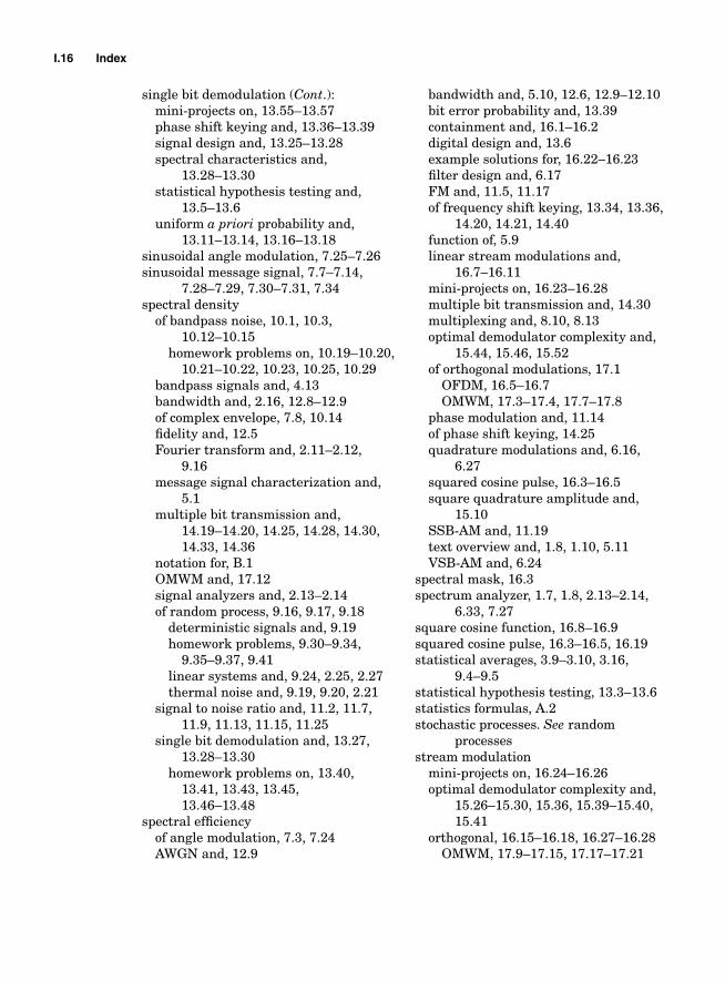
I.16 Index
single bit demodulation (Cont.):mini-projects on, 13.55–13.57phase shift keying and, 13.36–13.39signal design and, 13.25–13.28spectral characteristics and,
13.28–13.30statistical hypothesis testing and,
13.5–13.6uniform a priori probability and,
13.11–13.14, 13.16–13.18sinusoidal angle modulation, 7.25–7.26sinusoidal message signal, 7.7–7.14,
7.28–7.29, 7.30–7.31, 7.34spectral density
of bandpass noise, 10.1, 10.3,10.12–10.15
homework problems on, 10.19–10.20,10.21–10.22, 10.23, 10.25, 10.29
bandpass signals and, 4.13bandwidth and, 2.16, 12.8–12.9of complex envelope, 7.8, 10.14fidelity and, 12.5Fourier transform and, 2.11–2.12,
9.16message signal characterization and,
5.1multiple bit transmission and,
14.19–14.20, 14.25, 14.28, 14.30,14.33, 14.36
notation for, B.1OMWM and, 17.12signal analyzers and, 2.13–2.14of random process, 9.16, 9.17, 9.18
deterministic signals and, 9.19homework problems, 9.30–9.34,
9.35–9.37, 9.41linear systems and, 9.24, 2.25, 2.27thermal noise and, 9.19, 9.20, 2.21
signal to noise ratio and, 11.2, 11.7,11.9, 11.13, 11.15, 11.25
single bit demodulation and, 13.27,13.28–13.30
homework problems on, 13.40,13.41, 13.43, 13.45,13.46–13.48
spectral efficiencyof angle modulation, 7.3, 7.24AWGN and, 12.9
bandwidth and, 5.10, 12.6, 12.9–12.10bit error probability and, 13.39containment and, 16.1–16.2digital design and, 13.6example solutions for, 16.22–16.23filter design and, 6.17FM and, 11.5, 11.17of frequency shift keying, 13.34, 13.36,
14.20, 14.21, 14.40function of, 5.9linear stream modulations and,
16.7–16.11mini-projects on, 16.23–16.28multiple bit transmission and, 14.30multiplexing and, 8.10, 8.13optimal demodulator complexity and,
15.44, 15.46, 15.52of orthogonal modulations, 17.1
OFDM, 16.5–16.7OMWM, 17.3–17.4, 17.7–17.8
phase modulation and, 11.14of phase shift keying, 14.25quadrature modulations and, 6.16,
6.27squared cosine pulse, 16.3–16.5square quadrature amplitude and,
15.10SSB-AM and, 11.19text overview and, 1.8, 1.10, 5.11VSB-AM and, 6.24
spectral mask, 16.3spectrum analyzer, 1.7, 1.8, 2.13–2.14,
6.33, 7.27square cosine function, 16.8–16.9squared cosine pulse, 16.3–16.5, 16.19statistical averages, 3.9–3.10, 3.16,
9.4–9.5statistical hypothesis testing, 13.3–13.6statistics formulas, A.2stochastic processes. See random
processesstream modulation
mini-projects on, 16.24–16.26optimal demodulator complexity and,
15.26–15.30, 15.36, 15.39–15.40,15.41
orthogonal, 16.15–16.18, 16.27–16.28OMWM, 17.9–17.15, 17.17–17.21

Index I.17
spectral efficiency and, 16.21–16.22spectral shaping of, 16.7–16.11
systems engineering, 1.2–1.3. See alsospecific subject matter
Taylor series, 7.18telegraph, 1.1, 1.4, 8.17–8.18telephone
AWGN and, 12.14bandpass signals and, 4.2DTMF and, 12.11–12.12, 14.32–14.33history of communications and, 1.1multiplexing and, 8.17, 8.18OCDM and, 15.23OFDM and, 15.16OMWM and, 17.9spectral mask and, 16.2
televisionanalog communication and, 5.1, 5.4,
8.9bandwidth efficiency of, 5.11color signals and, 4.19error vector magnitude and, 16.13history of communications and, 1.1multiplexing and, 8.17noncoherent demodulation and, 6.27quadrature modulation and, 6.16,
6.19spectral containment and, 16.1–16.2
termination, 17.3theory. See communication theorythermal noise, 9.1, 9.19–9.21. See also
random processestime signals, 2.6total probability theorem, 3.4, 3.15transatlantic communication, 1.2transcendental functions, A.1–A.2translation and dilation theorem,
2.11transmission, analog, 5.5–5.8transmission efficiency, 5.9–5.10, 6.11,
11.7, 11.11, 11.14, 11.17transmitted reference based
demodulation, 6.23–6.27trapezoidal rule, 2.27trellis coded modulation (TCM), 17.4,
17.23–17.26, 17.32trigonometric formulas, A.1
undersea cables, 1.2Ungerboeck, Gottfried, 17.5uniform a priori probability, 13.11–13.14,
13.16–13.18union bound, 14.10
Euclidian distance and, 14.12–14.14example solutions and, 15.49homework problems, 14.28–14.29,
14.32, 14.33, 14.35, 14.36, 14.40linear modulation and, 15.8,
15.32–15.33for MFSK, 14.19, 14.21for MPSK, 14.23–14.24, 14.25, 14.26OMWM and, 17.23, 17.33quadrature amplitude modulation and,
15.31signal to noise ratio and, 14.15–14.16word error probability and,
14.10–14.12, 14.37
Varaldi, J., 17.5, 17.30, 17.33variable phase shift keying (VPSK),
14.30vector diagram, 4.7–4.9
analog fidelity and, 11.10of angle modulation and, 7.35of DSB-AM, 6.7error vector magnitude and, 16.13of frequency shift keying, 13.31homework problems on, 7.28–7.29,
7.31, 7.34–7.35, 17.36of LC-AM, 6.14–6.15of OFDM, 15.17of orthogonal stream modulations,
16.15–16.16, 16.17of phase shift keying, 13.36of SSB-AM, 6.23–6.24phase modulation and, 7.21text overview and, 1.8
vector signal analyzer, 1.7, 1.8, 4.8, 16.10,16.14
vestigial frequency, 6.18vestigial sideband amplitude modulation
(VSB-AM), 6.27angle modulation and, 7.24complex envelope of, 6.17complexity and, 11.19filter design of, 6.17–6.19

I.18 Index
vestigial sideband amplitude (Cont.):function of, 6.16–6.17homework problems on, 6.32–6.33,
6.35,13.42modulator for, 6.22–6.23
Viterbi, Andrew, 1.6, 17.8voiceband modem, 12.10voltage controlled oscillator (VCO), 7.6,
7.30–7.31, 8.1, 8.4
Watts, 2.4weak law of large numbers (WLLN),
9.4–9.5Wiener-Khinchin theorem, 9.17–9.18WiPhy, 1.5wireless communication
analog modulation and, 1.9convolution codes and, 17.23, 17.39energy efficiency and, 12.8history of communication and, 1.1, 6.4homework problems, 14.30,
14.35–14.36, 15.36, 15.41
OFDM and, 15.16, 15.18, 16.14physical layering and, 1.5
word error probabilitydemodulation fidelity and, 14.9–14.10of DTMF, 14.33linear modulation and, 15.6, 15.8, 15.9,
15.10homework problems on, 15.32–15.33,
15.42–15.43, 15.45MAPWD and, 14.4of MFSK, 14.18, 14.24–14.25, 15.46of MPSK, 14.28, 14.29, 15.38, 16.23of orthogonal modulation, 14.27,
15.37–15.38, 15.15–15.16OMWM, 17.7, 17.23, 17.25, 17.30,
17.34, 17.35of pulse position modulation, 14.35,
15.41of QAM, 15.31, 15.47of QPSK, 15.48signal design and, 14.16union bound and, 14.10, 14.12, 14.37