Fundamental Matrix / Image Rectification

COMPSCI 773 S1 T VISION GUIDED CONTROL

A/P Georgy Gimel’farb

COMPSCI 773 1

Epipolar Geometry

Epipoles

•  Ol,Or - projection centres –  Origins of the reference frames

–  fl, fr - focal lengths of cameras

•  πl, πr - image planes

–  3D reference frame for each camera: Z-axis = the optical axis

Pl=[Xl,Yl,Zl]T, Pr=[Xr,Yr,Zr]T - the same 3D point P in the reference frames

pl=[xl ,yl, zl =fl]T, pr=[xr,yr, zr =fr]T

- projections of P onto the image planes

COMPSCI 773 2

Basics of Epipolar Geometry

•  Reference frames of the left and right cameras - related via the extrinsic parameters –  Translation vector T = (Or - Ol) and a rotation matrix R

defining a rigid transformation in 3-D space, given a 3-D point P, between Pl and Pr: Pr = R(Pl - T)

•  Epipoles el and er - the points at which the line through the centres of projection intersects the image planes –  Left epipole - the image of the right projection centre –  Right epipole - the image of the left projection centre –  Canonical geometry: the epipole is at infinity of the baseline

COMPSCI 773 3

Basics of Epipolar Geometry

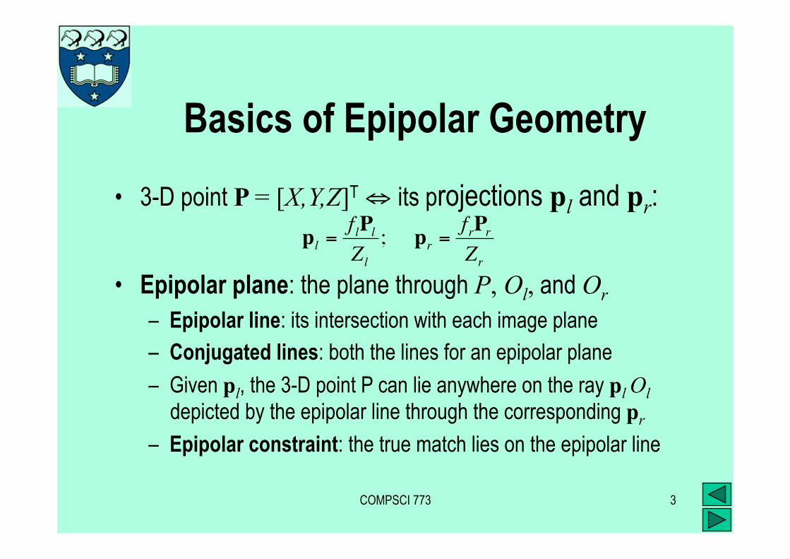
•  3-D point P = [X,Y,Z]T ⇔ its projections pl and pr:

•  Epipolar plane: the plane through P, Ol, and Or –  Epipolar line: its intersection with each image plane

–  Conjugated lines: both the lines for an epipolar plane

–  Given pl, the 3-D point P can lie anywhere on the ray pl Ol depicted by the epipolar line through the corresponding pr

–  Epipolar constraint: the true match lies on the epipolar line

€

pl =flPlZl

; pr =f rPrZr

COMPSCI 773 4

Basics of Epipolar Geometry

•  All epipolar lines go through the epipole – With the exception of the epipole, only one epipolar line goes

through any image point

– Mapping between points on one image and corresponding epipolar lines on the other image ⇒ the 1-D search region

–  Rejection of false matches due to occlusions

–  Corresponding points must lie on conjugated epipolar lines

•  The obvious question: how to estimate the epipolar geometry, i.e. determine the ‘point-to-line’ mapping for images

COMPSCI 773 5

The Essential Matrix, E

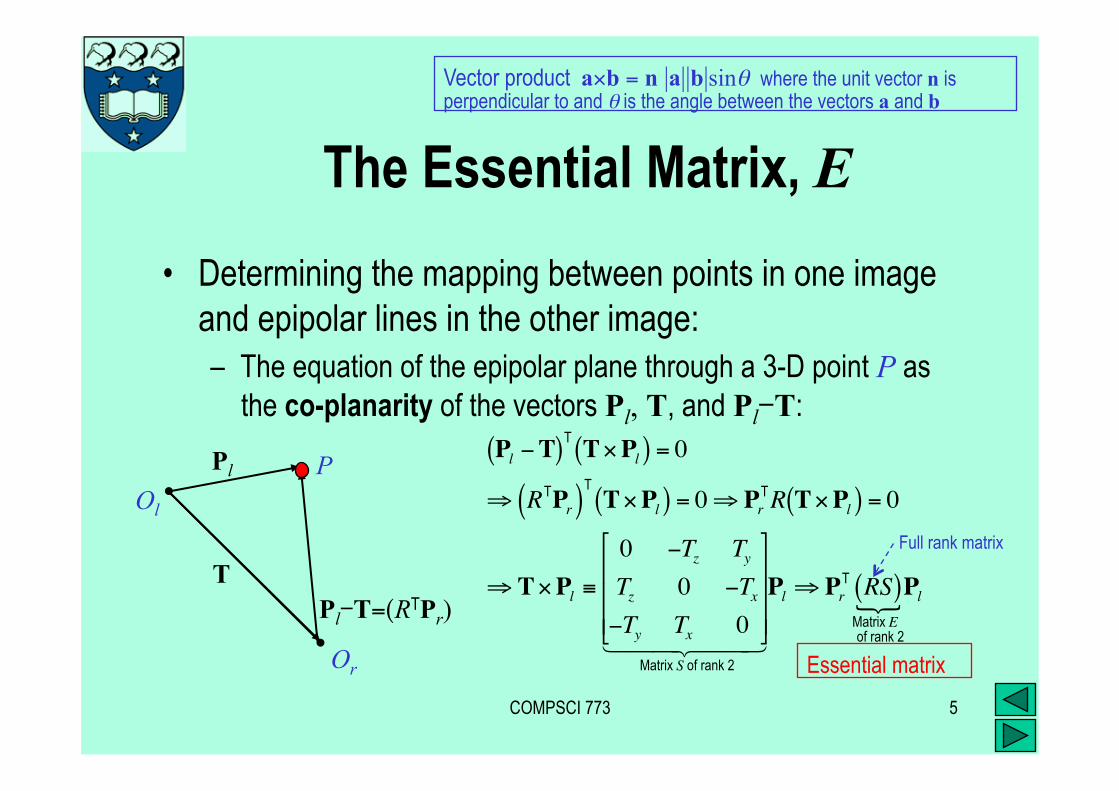
•  Determining the mapping between points in one image and epipolar lines in the other image: –  The equation of the epipolar plane through a 3-D point P as

the co-planarity of the vectors Pl, T, and Pl-T:

Pl

T Pl-T=(RTPr)

€

Pl −T( )T T×Pl( ) = 0

⇒ RTPr( )TT×Pl( ) = 0⇒ Pr

TR T×Pl( ) = 0

⇒ T×Pl ≡0 −Tz TyTz 0 −Tx−Ty Tx 0

Matrix S of rank 21 2 4 4 3 4 4

Pl ⇒ PrT RS( )

Matrix E of rank 2

{Pl

Ol

Or

P

Vector product a×b = n |a||b|sinθ where the unit vector n is perpendicular to and θ is the angle between the vectors a and b

Essential matrix

Full rank matrix

COMPSCI 773 6

The Essential Matrix, E

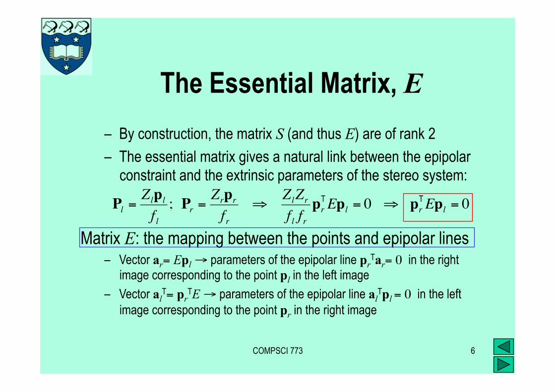
–  By construction, the matrix S (and thus E) are of rank 2

–  The essential matrix gives a natural link between the epipolar constraint and the extrinsic parameters of the stereo system:

Matrix E: the mapping between the points and epipolar lines –  Vector ar= Epl → parameters of the epipolar line pr

Tar= 0 in the right image corresponding to the point pl in the left image

–  Vector alT= pr

TE → parameters of the epipolar line alTpl = 0 in the left

image corresponding to the point pr in the right image

€

Pl =Zlplf l

; Pr =Zrprf r

⇒ ZlZr

f l frpr

TEpl = 0 ⇒ prTEpl = 0

COMPSCI 773 7

The Fundamental Matrix, F

•  The mapping “points ↔ epipolar lines” can be obtained from corresponding points only –  No prior information on the stereo system!

•  Points pl, pr in pixel and pl, pr in camera coordinates:

€

p l ≡x ly l1

= Mlpl; p r ≡x ry r1

= Mrpr ⇔ pl = Ml−1p l; pr = Mr

−1p r

⇒ p rT Mr

−T EMl−1

Fundamental matrix F

1 2 4 3 4 p l ⇒ p r

TFp l Ml and Mr - matrices of the intrinsic camera parameters

COMPSCI 773 8

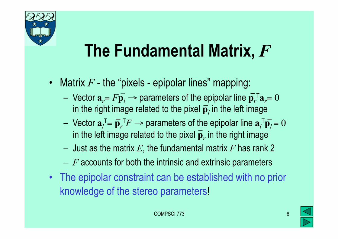
The Fundamental Matrix, F

•  Matrix F - the “pixels - epipolar lines” mapping: –  Vector ar= Fpl → parameters of the epipolar line pr

Tar= 0 in the right image related to the pixel pl in the left image

–  Vector alT= pr

TF → parameters of the epipolar line alTpl = 0

in the left image related to the pixel pr in the right image –  Just as the matrix E, the fundamental matrix F has rank 2

– F accounts for both the intrinsic and extrinsic parameters

•  The epipolar constraint can be established with no prior knowledge of the stereo parameters!

COMPSCI 773 9

The Eight-point Algorithm

•  n ≥ 8 corresponding points in the images are known –  Each correspondence i - a homogeneous linear equation:

–  If the n points do not form a degenerate configuration, the 9 entries of F are given by the non-trivial solution of this homogeneous linear system

€

p r,iT Fp l,i = 0⇒ x r,i y r,i 1[ ]

F11 F12 F13

F21 F22 F23

F31 F32 F33

x l,iy l,i1

= 0

⇒ x r,ix l ,iF11 + x r,iy l ,iF12 + x r,iF13 + y r,ix l,iF21 + y r,iy l,iF22

+ y r,iF23 + x l ,iF31 + y l,iF32 + F33 = 0

COMPSCI 773 10

The Eight-point Algorithm

–  Since the system is homogeneous, the solution is unique up to a signed scaling factor

–  Typically, n > 8, so that the system is over-determined, and its solution is obtained by singular value decomposition (SVD) related techniques

•  A - the system’s matrix n × 9:

€

A =

x r,1x l,1 x r,1y l,1 x r,1 y r,1x l ,1 y r,1y l ,1 y r,1 x l ,1 y l,1 1M M M M M M M M M

x r,n x l,n x r,n y l,n x r,n y r,n x l ,n y r,n y l ,n y r,n x l ,n y l,n 1

COMPSCI 773 11

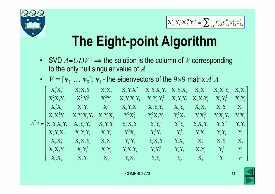
The Eight-point Algorithm •  SVD A=UDV

T ⇒ the solution is the column of V corresponding to the only null singular value of A

•  V = [v1 … v9]; vi - the eigenvectors of the 9×9 matrix ATA

€

ATA =

X r2X l

2 X r2X lYl X r

2X l X rYrX l2 X rYrX lYl X rYrX l X rX l

2 X rX lYl X rX l

X r2X lYl X r

2 Yl2 X r

2Yl X rYrX lYl X rYr Yl2 X rYrYl X rX lYl X rYl

2 X rYlX r2X l X r

2Yl X r2 X rYrX l X rYrYl X rYr X rX l X rYl X r

X rX l2Yr X rYrX lYl X rYrX l Yr

2X l2 Yr

2X lYl Yr2X l YrX l

2 YrX lYl YrX l

X rYrX lYl X rYr Yl2 X rYrYl Yr

2X lYl Yr2Yl

2 Yr2Yl YrX lYl YrYl

2 YrYlX rYrX l X rYrYl X rYr Yr

2X l Yr2Yl Yr

2 YrX l YrYl YrX rX l

2 X rX lYl X rX l Yr2Yl YrX lY YrX l X l

2 X lYl X l

X rX lYl X rYl2 X rYl YrX lYl YrYl

2 YrYl X lYl Yl2 Yl

X rX l X rYl X r YrX l YrYl Yr X l Yl n

€

X rαYr

γX lβYl

δ ≡ xr,iα yr,i

β xl,iγ xl ,i

δ

i=1

n∑

COMPSCI 773 12

The Eight-point Algorithm

•  Due to noise, the solution is the column of V associated with the least singular value

•  The estimated fundamental matrix Fest is almost always non-singular, i.e. is full rank (3) rather than the expected rank 2 –  The singularity is enforced by adjusting the entries of Fest:

•  The SVD Fest = UDV T

•  Set the smallest singular value in the diagonal matrix D to zero to obtain the corrected matrix D′

•  The corrected estimate: F ′ = UD′V T

COMPSCI 773 13

To Avoid Numerical Instabilities:

•  Coordinates of the corresponding points have to be normalised to make entries of A of comparable size –  Translate the two coordinates of each point to the centroid of

each data set:

–  Scale the norm of each point so that the average norm over the data set is 1:

€

pi =

xiyi1

⇒ ′ p i =

xi −mx( ) dyi −my( ) d

1

⇔ ′ p i = Hpi ≡

1 d 0 −mx d0 1 d −my d0 0 1

xiyi1

€

mx = 1n xii=1

n∑ ; my = 1

n yii=1

n∑

€

d = 1n 2

xi −mx( )2 + yi −my( )2

i∑

COMPSCI 773 14

Stable Eight-Point Algorithm

•  Input: n pixel-to-pixel correspondences

•  Data normalisation:

€

pl,i = xl,i yl ,i 1[ ]T; pr,i = xr,i yr,i 1[ ]T( ) : i =1,K,n{ }

€

′ p l,i = Hlpl ,i; ′ p r,i = Hrpr,i( ) : i =1,K,n{ }

€

Hl =

1dl

0 −ml,x

dl0 1

dl−ml,y

dl0 0 1

; Hl−1 =

dl 0 ml,x

0 dl ml,y

0 0 1

; Hr =

1dr

0 −mr,x

dr0 1

dr−mr,y

dr0 0 1

; Hr−1 =

dr 0 mr,x

0 dr mr,y

0 0 1

COMPSCI 773 15

Stable Eight-Point Algorithm

•  SVD A = UDV T of the n×9 matrix A for the system of

n linear equations; n ≥ 8 (over-determined for n > 8):

€

′ p r,iT ′ F ′ p l,i = 0 ⇒ ′ x r,i, ′ y r,i,1[ ]

F1 F2 F3

F4 F5 F6

F7 F8 F9

′ x l,i′ y l,i1

= 0 ⇒ a iTf = 0 : i =1,2,...,n{ }

Af = 0 where A =

a1T

a2T

M

anT

; a iT = ′ x l,i ′ x r,i, ′ y l ,i ′ x r,i, ′ x r,i, ′ x l,i ′ y r,i, ′ y l ,i ′ y r,i, ′ y r,i, ′ x l,i, ′ y l,i,1[ ]; f =

F1

F2

M

F9

COMPSCI 773 16

Stable Eight-Point Algorithm

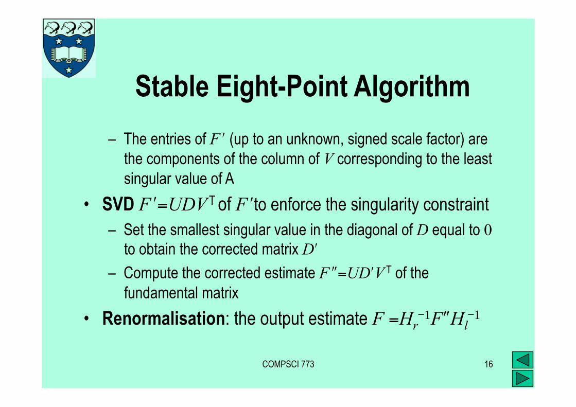
–  The entries of F ′ (up to an unknown, signed scale factor) are the components of the column of V corresponding to the least singular value of A

•  SVD F ′=UDV T of F ′to enforce the singularity constraint

–  Set the smallest singular value in the diagonal of D equal to 0 to obtain the corrected matrix D′

–  Compute the corrected estimate F ″=UD′V T of the

fundamental matrix

•  Renormalisation: the output estimate F =Hr-1F″Hl

-1

COMPSCI 773 17

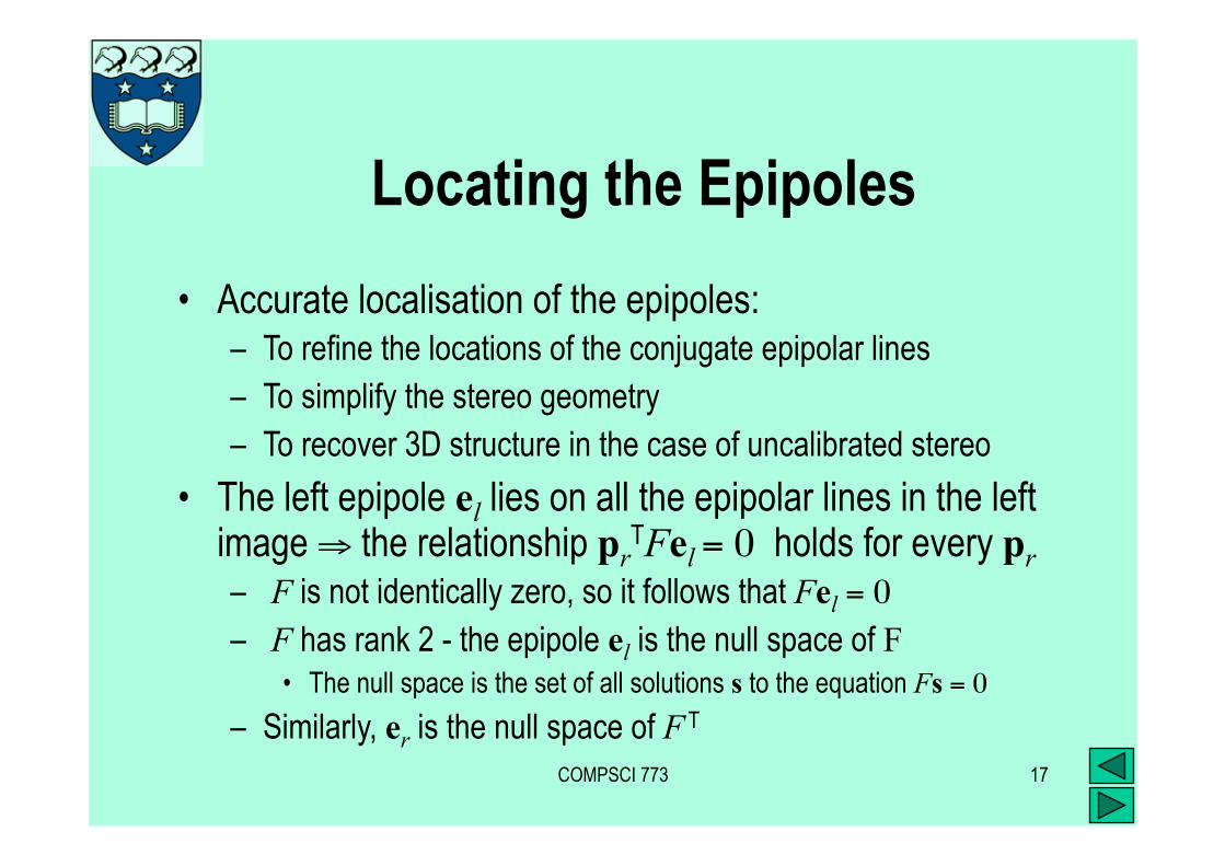
Locating the Epipoles

•  Accurate localisation of the epipoles: –  To refine the locations of the conjugate epipolar lines –  To simplify the stereo geometry –  To recover 3D structure in the case of uncalibrated stereo

•  The left epipole el lies on all the epipolar lines in the left image ⇒ the relationship pr

TFel = 0 holds for every pr –  F is not identically zero, so it follows that Fel = 0 –  F has rank 2 - the epipole el is the null space of F

•  The null space is the set of all solutions s to the equation Fs = 0

–  Similarly, er is the null space of F T

COMPSCI 773 18

Algorithm to Locate Epipoles

•  Input: the fundamental matrix F

•  SVD F = UDV T

–  The epipole el : the column of V corresponding to the null singular value

–  The epipole er : the column of U corresponding to the null singular value

€

F =

0 0 00 0 10 1 0

=

0 1 0120 1

2120 −1

2

U1 2 4 3 4

1 0 00 0 00 0 −1

D1 2 4 3 4

0 12

12

1 0 00 1

2−12

V T

1 2 4 3 4

⇒ e l = er =

100

COMPSCI 773 19

Rectification of Stereo Images

Rectification - a transformation (warping) of each image: pairs of conjugate epipolar lines become collinear and parallel to one of the image axes (typically, x-axis) –  The 1-D search for correspondence after rectification

–  Computation: by using the known intrinsic parameters of the camera and extrinsic parameters of the stereo system

–  The rectified images are thought of as acquired by a new stereo rig obtained by rotating the original cameras around their optical centres

COMPSCI 773 20

Rectification of a Stereo Pair P

Or

Ol

The epipolar lines associated to a 3-D point P in the original cameras become collinear in the rectified cameras

The original cameras can be in any position, and the optical axes may not intersect

COMPSCI 773 21

Rectification of a Stereo Pair

COMPSCI 773 22

Assumptions and Basic Steps

•  Assumptions for both cameras without losing generality: (1) The origin of the image reference frame in the principal point

(the trace of the optical axis) and (2) the same focal length f •  Steps of rectification

(1) Rotate the left camera to make its image plane parallel to the baseline of the system (the epipole goes to infinity along the x-axis)

(2) Apply the same rotation to the right camera to recover the original geometry and then (3) rotate the right camera by R

(4) Adjust the scale in both camera reference frames

COMPSCI 773 23

Rotation Matrix Rrect for Step 1

•  A triple of mutually orthogonal unit vectors e1, e2, and e3 –  An arbitrary choice due to an under-constrained problem

–  The epipole e1 coincides with the direction of translation (as the image centre is in the origin)

€

Rrect =

e1T

e2T

e3T

where e1 =

TT

=1

Tx2 + Ty

2 + Tz2

TxTyTz

; e2 =

e1 × 0,0,1[ ]T

e1 × 0,0,1[ ]T =1

Tx2 + Ty

2

−TyTx0

;

e3 = e1 × e2 =1

Tx2 + Ty

2( ) Tx2 + Ty2 + Tz

2( )

−TxTz−TyTzTx

2 + Ty2

The direction vector of the optical axis

COMPSCI 773 24

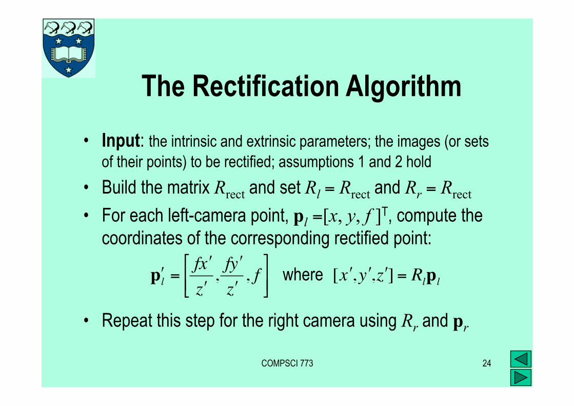
The Rectification Algorithm

•  Input: the intrinsic and extrinsic parameters; the images (or sets of their points) to be rectified; assumptions 1 and 2 hold

•  Build the matrix Rrect and set Rl = Rrect and Rr = Rrect

•  For each left-camera point, pl =[x, y, f ]T, compute the coordinates of the corresponding rectified point:

•  Repeat this step for the right camera using Rr and pr

€

′ p l =f ′ x ′ z

, f ′ y ′ z

, f

where [ ′ x , ′ y , ′ z ] = Rlpl