ORIGINALARTICLE

Functionally relevant climate variablesfor arid lands: a climatic water deficitapproach for modelling desert shrubdistributionsThomas E. Dilts1*, Peter J. Weisberg1, Camie M. Dencker1 and

Jeanne C. Chambers2

1Department of Natural Resources and

Environmental Science, University of Nevada

Reno, 1664 N. Virginia St. Reno, Nevada

89557, USA, 2U.S. Forest Service, Rocky

Mountain Research Station, 920 Valley Road

Reno, NV 89512, USA

*Correspondence: Thomas E. Dilts, 1664 N.

Virginia St. Reno, Nevada 89557, USA.

E-mail: tdilts@cabnr.unr.edu

ABSTRACT

Aim We have three goals. (1) To develop a suite of functionally relevant cli-

mate variables for modelling vegetation distribution on arid and semi-arid

landscapes of the Great Basin, USA. (2) To compare the predictive power of

vegetation distribution models based on mechanistically proximate factors

(water deficit variables) and factors that are more mechanistically removed

from a plant’s use of water (precipitation). (3) To quantify the climate gradi-

ents that control shrub distributions in a cold desert environment.

Location The central basin and range ecoregion of the western USA

(36–42°N).

Methods We used a modified Thornthwaite method to derive monthly water

balance variables and to depict them using a water balance climograph. Eigh-

teen variables were calculated from the climograph, representing different com-

ponents of the seasonal water balance. These were used in boosted regression

tree models to derive distribution models for 18 desert shrub species. The

water balance approach was compared with an approach that used bioclimatic

variables derived from the PRISM (Parameter-elevation Relationships on Inde-

pendent Slopes Model) climate data.

Results The water balance and bioclimatic approaches yielded models with simi-

lar performance in predicting the geographical distribution of most shrub species.

Cumulative annual climatic water deficit was consistently the most important

water balance variable for predicting shrub type distributions, although predictions

were improved by the inclusion of variables that describe the seasonal distribution

of water balance such as water supply in the spring, fall actual evapotranspiration,

monsoonality and summer decline in actual evapotranspiration.

Main conclusions The water balance and bioclimatic approaches to species

distribution modelling both yielded similar prediction accuracies. However, the

water balance approach offers advantages over the bioclimatic approach

because it is mechanistically derived to approximate physical processes impor-

tant for plant growth.

Keywords

Climatic water deficit, climograph, cold desert shrubs, gradient analysis, Great

Basin, mechanistic model, PRISM, species distribution modelling, water

balance, western USA.

INTRODUCTION

A long tradition of vegetation modelling originates from gra-

dient analysis studies. It is well established that vegetation

distribution responds to gradients of temperature, moisture,

and to a lesser degree, soil nutrients and geology (e.g. Whit-

taker & Niering, 1965; Franklin, 1995). However, in arid and

semi-arid regions of the world, water relations are expected

ª 2015 John Wiley & Sons Ltd http://wileyonlinelibrary.com/journal/jbi 1doi:10.1111/jbi.12561

Journal of Biogeography (J. Biogeogr.) (2015)

to play the dominant role in structuring plant communities.

In mountainous arid regions, precipitation and temperature

often vary consistently and inversely along the same gradient

of elevation due to orographic and adiabatic effects. As a

result, ecologists have characterized the vegetation of arid

ecosystems as varying along a single moisture gradient

(Whittaker, 1967) or have relied upon relationships with

soils and topography to predict the distribution of plant spe-

cies (West, 1983). The resulting models may be difficult to

generalize to areas that have differing relationships between

climate and topography. In climates in which the majority of

precipitation falls outside the growing season, simple models

may underestimate the role that soil serves to store water

received during the wet season for use by plants during the

growing season. Similarly, vegetation models relying upon

topographic variables alone are not expected to be predictive

under climate change scenarios, because topographic vari-

ables remain static while climatic variables change (Dyer,

2009). Because of the differing predictions for future precipi-

tation and temperature regimes across space, a modelling

approach that can functionally separate the water balance

components (precipitation, evapotranspiration, soil water

balance) may prove useful for predicting individual species

responses to climate change.

Identifying species–environment relationships using the

most direct causal variables is one of the fundamental chal-

lenges in ecology (Guisan & Zimmermann, 2000; Austin,

2002). The climatic water deficit (CWD) approach has

been proposed as an ecologically functional description of

climate influences that limit plant distributions (Stephen-

son, 1990, 1998). This approach uses water balance models

and offers advantages for modelling species–environment

relationships over traditional empirical ‘climate envelope’

models based purely on climate variables (precipitation and

temperature) that use proxies for variables that are more

functionally related to plant growth, including soil water

content and soil water deficit. Directly including these criti-

cal variables in distribution models may increase their pre-

dictive capabilities and allow further insights regarding

factors that limit establishment, growth and mortality

(Piedallu et al., 2013; Das et al., 2013). At the level of the

individual plant, what matters most is likely to be the

amount of water in its rooting zone over the course of the

time period when the plant most needs water, rather than

the long-term average amount of precipitation at a regional

level.

The temporal availability of moisture also is an important

determinant of the distribution of major vegetation physiog-

nomic types at local to continental scales (Stephenson,

1990). For example, both the Great Plains and Great Basin

regions of the USA have similar annual precipitation and

temperature regimes but the former is dominated by grami-

noids while the latter is dominated by shrubs. This difference

is attributed to the lack of summer precipitation in the Great

Basin which favours deep-rooted shrub species over grami-

noids (Paruelo & Lauenroth, 1996). The climatic water defi-

cit (CWD) approach, based upon a Thornthwaite water

balance model (Lutz et al., 2010), is well suited for repre-

senting the seasonal and temporal availability of moisture

because it can be calculated at monthly time steps, tracking

previous conditions and accounting for temporal lags

between water availability and evaporative demand. The

CWD approach can also include development of climographs

(sensu Stephenson, 1998) that allow visual assessment of vari-

ables such as water supply and potential and actual evapo-

transpiration and provide a more nuanced view of

vegetation–climate relationships. In contrast, the bioclimatic

approach does not explicitly account for water storage in the

soil or snowpack and considers temperature and precipita-

tion as acting independently rather than interacting to affect

water balance at a site.

Shrubs in the cold desert of the Great Basin of the western

USA provide an excellent case for testing the water deficit

approach and comparing it with traditional approaches using

climate data based on precipitation and temperature. Desert

shrubs have received less attention than trees with respect to

vegetation–climate modelling (e.g. Lutz et al., 2010; Crim-

mins et al., 2011). Desert shrub distributions are strongly

influenced by water availability and demand and vary with

subtle changes in soil texture, soil depth and aspect (Franklin,

1995; Miller & Franklin, 2002, 2006), which can be repre-

sented in climate water deficit models. Here, we address

three sets of research questions:

1. Do species distribution models developed from water def-

icit variables perform better in terms of model fit compared

to distribution models developed from commonly used bio-

climatic variables?

2. Are species distribution models developed from water

deficit variables more transferable in space compared to dis-

tribution models developed from commonly used bioclimatic

variables?

3. How are shrub species distributed along ecological

gradients and which gradients are most predictive across

species?

Previous exercises in species distribution modelling have

demonstrated the predictive power of the annual water defi-

cit and actual evapotranspiration for species distribution

modelling (e.g. Stephenson, 1998; Lutz et al., 2010; Piedallu

et al., 2013). We refine this general approach by developing

new indices that more fully describe differences in demand

and timing of water availability based on the water deficit

climograph, and by incorporating these indices into our pre-

dictive models. We expect that variables quantifying annual

levels of water availability and demand will be generally pre-

dictive, but that other variables that quantify the timing and

seasonality of water availability and demand will help to dis-

tinguish among shrub species with differing phenology, sea-

sonal patterns of water use and rooting depths. We compare

models based on standard bioclimatic variables to models

that use water deficit variables to determine whether a water

deficit approach offers an advantage in predicting shrub type

distributions. We expect the largest advantages of using

Journal of Biogeographyª 2015 John Wiley & Sons Ltd

2

T. E. Dilts et al.

water deficit variables for lower-elevation shrub species that

are most water-limited, and the least advantage for higher-

elevation shrub species with greater water availability

but that may be temperature-limited due to short growing

seasons.

MATERIALS AND METHODS

Study area

Our study area is the entire Great Basin of the USA

(451,112 km2) (Fig. 1), encompassing the majority of the

Central Basin and Range province (Omernik, 1987). Land-

form morphology is dominated by north–south trending

fault block mountain ranges alternating with broad alluvial

valleys. Elevations range from �83 to 4383 m. The climate is

arid to semi-arid and average precipitation is 30.6 cm per

year. Topographic effects on precipitation are strong, result-

ing in annual precipitation as high as 205 cm in mountain-

ous areas and as low as 6.6 cm in the most arid sites. Winter

months receive roughly three times as much precipitation as

summer months, but, the eastern and southernmost portions

of the study area are influenced by summer monsoonal

storms.

Much of the region is dominated by deeply rooted shrub

species. The lowest elevations are characterized by salt desert

shrub communities and are dominated by shrub species such

as shadscale (Atriplex confertifolia (Pursh) Nutt.), four-wing

saltbush (Atriplex canescens (Pursh) Nutt.), winterfat

(Krascheninnikovia lanata (Pursh) A. Meeuse & Smit), and

black greasewood (Sarcobatus vermiculatus (Hook.) Torr).

Sagebrush communities dominated by Wyoming big sage-

brush (Artemisia tridentata Nutt. ssp. wyomingensis Beetle &

Young), interspersed with perennial grasses, occur at middle

elevations. At middle elevation sites with shallower or coarser

soils, black sagebrush (Artemisia nova A. Nelson) dominates

instead of Wyoming big sagebrush. At higher elevations

mountain big sagebrush (Artemisia tridentata ssp. vaseyana

(Rydb.) B. Boivin), low sagebrush (Artemisia arbuscula Nutt.)

and antelope bitterbrush (Purshia tridentata Pursh) commu-

nities co-occur with single-needle pinyon pine (Pinus mono-

phylla Torr. & Fr�em.) and Utah juniper (Juniperus

osteosperma (Torr.) Little) (Tables 1 & 2).

Shrub species data

Presence–absence data were derived from Southwest Regional

GAP Training Site Databases for Nevada and Utah (USDI,

2004a) for 18 of the most common desert shrub species

(Table 1). The number of occurrence points per species ran-

ged from 231 for four-wing saltbush to 3255 for Wyoming

big sagebrush and species prevalence ranged from 0.6% to

8% (Table 2). Occurrence points falling within areas classi-

fied as riparian by the Southwest Regional GAP Analysis

map (USDI, 2004b) were excluded, as were areas subject to

recent fires based on the Monitoring Trends in Burn Severity

dataset (USDA, 2009) and the Nevada Fire History Database

for 1981 to 2008 (USDI, 2008).

Environmental predictors

Climatic variables were derived from two primary sources.

Eleven standard bioclimatic variables (Table 3) that are com-

monly used in bioclimatic envelope modelling (Hijmans

et al., 2005) were derived from gridded PRISM (Parameter–elevation Relationships on Independent Slopes Model)

climate data (PRISM Group, 2007). Data from PRISM can

substantially improve climate predictions in topographically

heterogeneous regions compared to WorldClim and DayMet

products (Daly et al., 2008). Water deficit variables (Table 4)

were derived from a water balance model (Lutz et al., 2010)

that was implemented in ArcGIS version 10.1 (ESRI, 2012)

using custom scripts from Dilts (2015). The water balance

model used monthly gridded PRISM temperature and pre-

cipitation averages (PRISM Group, 2007) for the 1971 to

2000 time period at 800-m cell size, USDA gridded SSURGO

soils data (USDA, 2013) and a digital elevation model. For

areas where SSURGO data were unavailable (approximately

23% of study area), we used a constant soil water holding

capacity value of 100 mm which approximated the average

value of the study area.

A Thornthwaite water balance model was used to calculate

the following variables at monthly time steps: potential

evapotranspiration (PET), actual evapotranspiration (AET),

climatic water deficit (CWD), water supply (WS) and soil

water balance (SWB) (Lutz et al., 2010). PET represents the

amount of water that would be evaporated and transpired if

water were available. We follow the definitions of Stephenson

(1990, 1998) and Lutz et al. (2010) in which AET is defined

as evaporative water loss from a site covered by a hypotheti-

cal standard row crop, constrained by water availability. AET

can be thought to represent net primary productivity as it

considers the amount of water that is biologically useable,

given the simultaneous availability of both water and energy

(Stephenson, 1998). CWD is calculated as the difference

between PET and AET and represents the unmet evaporative

demand for water (Stephenson, 1990). Water supply is calcu-

lated as the sum of snowmelt and rain. Soil water balance is

calculated as water supply minus PET plus the previous

month’s soil water constrained by the maximum soil water

holding capacity.

To represent seasonal temperature effects, growing degree-

days (GDD) was calculated as:

GDD ¼ Tmax þ Tmin

2� Tbase;

where Tbase was 5.56 °C and Tmax and Tmin were calculated

from PRISM climate data (PRISM Group, 2007). The water

balance model accounted for water storage in the snowpack

and soil (Lutz et al., 2010) and incorporated topographic

effects on solar radiation and potential evapotranspiration

Journal of Biogeographyª 2015 John Wiley & Sons Ltd

3

Modelling shrub distributions using a water balance approach

using the dimensionless heat-load index of McCune & Keon

(2002) following the method of Lutz et al. (2010). Although

the use of the heat-load index in the water balance allows for

predictions at the grain of the digital elevation model, we

retained the 800-m resolution for all water balance variables

to compare with the bioclimatic model.

Monthly outputs of water balance (PET, AET, CWD, WS,

SWB) and GDD were plotted as climographs (sensu Stephen-

son, 1998). Eighteen variables were calculated that described

the magnitude, duration and timing of water balance charac-

teristics (Fig. 2, and see Appendix S1 in Supporting Informa-

tion). Rather than use all monthly variables (6 variables 9

12 months = 72 variables), we used a data reduction proce-

dure (principal components analysis) to reduce multicollin-

earity and determine the dimensionality of the data (see

Appendix S2 for details). The following five bioclimatic vari-

ables were retained for modelling: mean annual temperature

(Temp), temperature annual range (TempRang), annual pre-

cipitation (Precip), precipitation of the driest month (Precip-

DryMo) and precipitation seasonality (PrecipSeas) (Table 3).

The following five water deficit variables were retained for

modelling: cumulative water deficit (CumlCWD), steepest

rate of decline of actual evapotranspiration (DeclAET), dif-

ference between actual evapotranspiration summer low and

fall peak (FallAET), positive difference in water supply

between August and June (monsoonality; Ws86c) and differ-

ence between water supply and AET during the spring

(WsAETSpr) (Table 4). Maps of predictor variables are

shown in Appendix S2.

Statistical analysis

We used boosted regression trees (Ridgeway, 2006) to calculate

separate distribution models for the 18 desert shrub species

using either the bioclimatic variables or water deficit variables.

The boosted regression trees method is one of the most useful

techniques for presence–absence species distribution model-

ling, because of the good predictive performance of the techni-

que compared to more traditional methods, such as

generalized linear models and classification and regression

trees, its ability to deal with interactions and nonlinear rela-

tionships, and its use of cross-validation to reduce over-fitting

(Elith et al., 2008). We used a tree complexity of three

(roughly equivalent to the interaction order) and set the learn-

ing rate to 0.005 to ensure that a minimum of 1000 trees were

generated for each species modelled.

Two methods were used to evaluate the models. First, the

Southwest Regional GAP database of occurrence points was

randomly partitioned into separate training (n = 27,248) and

validation (n = 13,624) datasets after the removal of riparian

and burned points, and the threshold-independent area

under the curve (AUC) of the receiver operating characteris-

tic (ROC) plot (Fielding & Bell, 1997) was calculated for the

validation dataset (TeAUC = ‘average test AUC’). Perfor-

mance measures for randomly partitioned data may be

inflated by spatial autocorrelation where the locations of

training and validation points are close to one another (Hij-

mans, 2012). Therefore, we adopted an approach in which

the study area was divided into four quadrants, models were

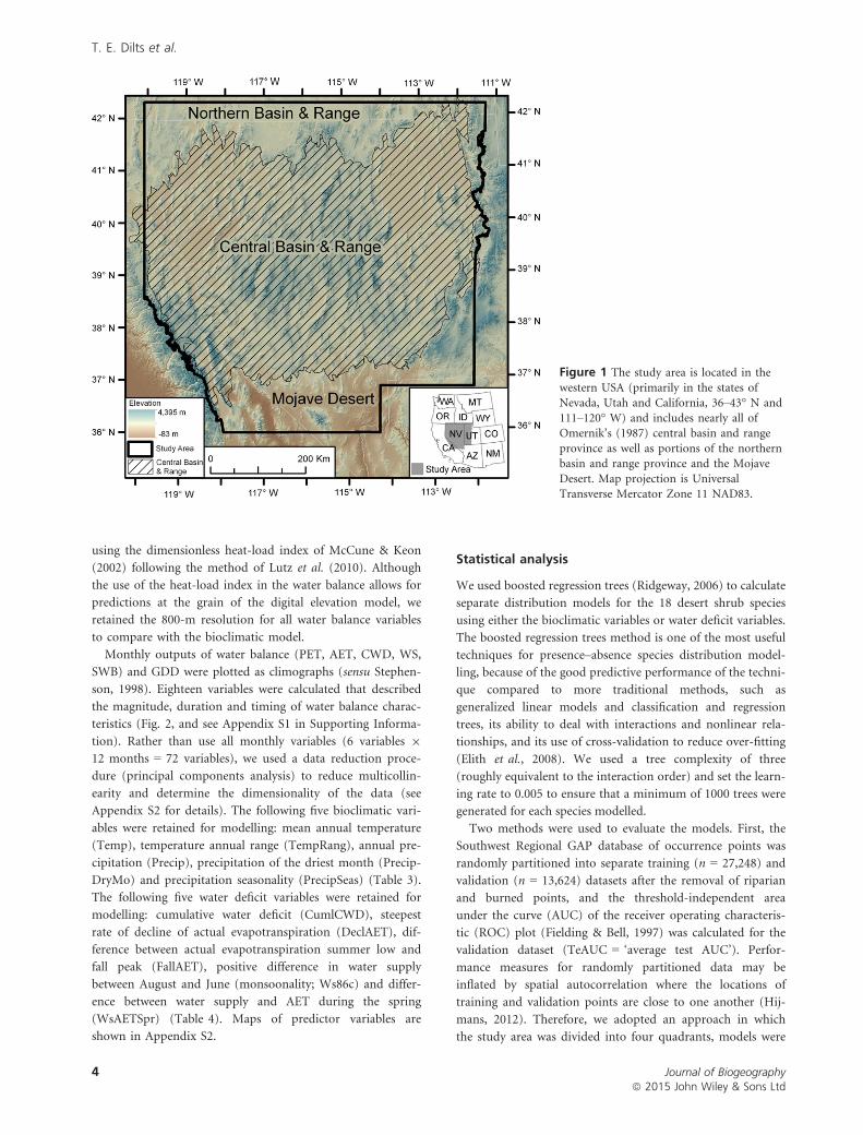
Figure 1 The study area is located in the

western USA (primarily in the states ofNevada, Utah and California, 36–43° N and

111–120° W) and includes nearly all ofOmernik’s (1987) central basin and range

province as well as portions of the northernbasin and range province and the Mojave

Desert. Map projection is UniversalTransverse Mercator Zone 11 NAD83.

Journal of Biogeographyª 2015 John Wiley & Sons Ltd

4

T. E. Dilts et al.

developed based on data from one quadrant and then

validated using the other three quadrants as independent test

data. This resulted in a total of 12 validation AUC values

that were then averaged (Radosavljevic & Anderson, 2014;

GeoAUC = ‘geographically partitioned AUC’).

We measured the tendency for model overfit by taking the

difference between average training AUC in each of the four

quadrants and average validation AUC for the validation

quadrants (Radosavljevic & Anderson, 2014). Predictive maps

were calculated at 800-m cell size for both types of models

and all 800-m pixels were used to calculate correlation coeffi-

cients between the CWD and bioclimatic model predictions.

The relative influence of each variable was calculated using

the method of Friedman (2001) as implemented using the R

package gbm (Ridgeway, 2006) where each variable’s influ-

ence is based on the number of times it is selected for split-

ting the regression tree weighted by the squared

improvement to the model as the result of the split averaged

over all regression trees (Elith et al., 2008). The relative

influence of all variables sum to 100%.

RESULTS

Climographs

The seasonal progression of site water balance varied consis-

tently among shrub species, many of which were clearly

distinguishable on the basis of their climographs (Fig. 3).

The most xeric sites were occupied by black greasewood

(Sarcobatus vermiculatus) and shadscale (Atriplex confertifolia)

and exhibited large cumulative climatic water deficits, a high

number of cumulative growing degree-days, and a small sea-

sonal spike in water supply that barely exceeded soil water

holding capacity. Black greasewood’s climograph closely

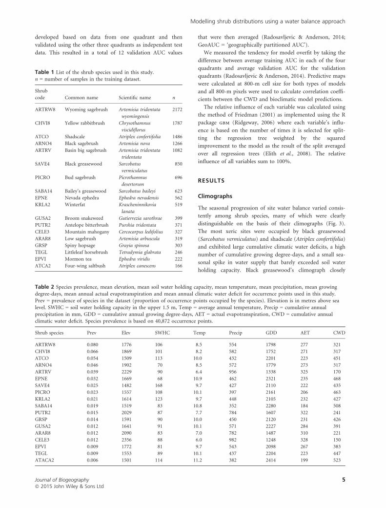
Table 1 List of the shrub species used in this study.

n = number of samples in the training dataset.

Shrub

code Common name Scientific name n

ARTRW8 Wyoming sagebrush Artemisia tridentata

wyomingensis

2172

CHVI8 Yellow rabbitbrush Chrysothamnus

viscidiflorus

1787

ATCO Shadscale Atriplex confertifolia 1486

ARNO4 Black sagebrush Artemisia nova 1266

ARTRV Basin big sagebrush Artemisia tridentata

tridentata

1082

SAVE4 Black greasewood Sarcobatus

vermiculatus

850

PICRO Bud sagebrush Picrothamnus

desertorum

696

SABA14 Bailey’s greasewood Sarcobatus baileyi 623

EPNE Nevada ephedra Ephedra nevadensis 562

KRLA2 Winterfat Krascheninnikovia

lanata

519

GUSA2 Broom snakeweed Gutierrezia sarothrae 399

PUTR2 Antelope bitterbrush Purshia tridentata 371

CELE3 Mountain mahogany Cercocarpus ledifolius 327

ARAR8 Low sagebrush Artemisia arbuscula 319

GRSP Spiny hopsage Grayia spinosa 303

TEGL Littleleaf horsebrush Tetradymia glabrata 246

EPVI Mormon tea Ephedra viridis 222

ATCA2 Four-wing saltbush Atriplex canescens 166

Table 2 Species prevalence, mean elevation, mean soil water holding capacity, mean temperature, mean precipitation, mean growing

degree-days, mean annual actual evapotranspiration and mean annual climatic water deficit for occurrence points used in this study.Prev = prevalence of species in the dataset (proportion of occurrence points occupied by the species). Elevation is in metres above sea

level. SWHC = soil water holding capacity in the upper 1.5 m, Temp = average annual temperature, Precip = cumulative annualprecipitation in mm, GDD = cumulative annual growing degree-days, AET = actual evapotranspiration, CWD = cumulative annual

climatic water deficit. Species prevalence is based on 40,872 occurrence points.

Shrub species Prev Elev SWHC Temp Precip GDD AET CWD

ARTRW8 0.080 1776 106 8.5 554 1798 277 321

CHVI8 0.066 1869 101 8.2 582 1752 271 317

ATCO 0.054 1509 113 10.0 432 2201 223 451

ARNO4 0.046 1902 70 8.5 572 1779 273 317

ARTRV 0.039 2229 90 6.4 956 1338 325 170

EPNE 0.032 1669 68 10.9 462 2321 235 468

SAVE4 0.025 1482 168 9.7 427 2110 222 435

PICRO 0.023 1557 108 10.1 397 2161 206 463

KRLA2 0.021 1614 123 9.7 448 2105 232 427

SABA14 0.019 1519 83 10.8 352 2280 184 508

PUTR2 0.015 2029 87 7.7 784 1607 322 241

GRSP 0.014 1591 90 10.0 450 2120 231 426

GUSA2 0.012 1641 91 10.1 571 2227 284 391

ARAR8 0.012 2090 83 7.0 782 1487 310 221

CELE3 0.012 2356 88 6.0 982 1248 328 150

EPVI 0.009 1772 81 9.7 543 2098 267 383

TEGL 0.009 1553 89 10.1 437 2204 223 447

ATACA2 0.006 1501 114 11.2 382 2414 199 523

Journal of Biogeographyª 2015 John Wiley & Sons Ltd

5

Modelling shrub distributions using a water balance approach

resembled that of shadscale, but had higher variability in most

water deficit variables and a less precipitous decline in AET

between May and July. Black sagebrush and Wyoming big

sagebrush occupied the intermediate portion of the dominant

moisture gradient. Black sagebrush had more variable spring

water supply in excess of PET, slightly higher variability in

growing degree-days, and slightly smaller average cumulative

CWD. Higher soil water holding capacity of Wyoming big

sagebrush sites allowed a lower cumulative water deficit and

higher cumulative AET than would be expected based on tem-

perature and precipitation alone (Table 2). Winterfat occupied

the lower to middle portion of the dominant moisture gradi-

ent with a slightly larger but more variable number of cumula-

tive growing degree-days, a smaller water supply in excess of

PET in the spring compared to Wyoming big sagebrush and

black sagebrush and larger cumulative annual water deficit.

On the mesic end of the dominant moisture gradient low

sagebrush and mountain big sagebrush had climographs with

smaller cumulative water deficit, a smaller number of cumu-

lative growing degree-days, and a spike in spring water sup-

ply that greatly exceeded PET. Mountain big sagebrush

differed from low sagebrush in that AET was more variable

among sites during the growing season.

Model performance of bioclimatic versus water

deficit models

Model performance was similar for both the bioclimatic and

water deficit approaches but varied greatly by species

(Table 5). Average test AUC was 0.818 for the bioclimatic

models (range 0.733–0.929) and 0.799 for the water deficit

models (range 0.718–0.915). When evaluated against geo-

graphically independent validation areas the AUC values

were, on average, 0.106 and 0.103 lower for bioclimatic and

water deficit models compared to the randomly partitioned

dataset. Mountain mahogany (Cercocarpus ledifolius)

remained the best predicted species when evaluated against

geographically independent validation data with an AUC of

0.865 and 0.883 for the bioclimatic and water deficit models.

Broom snakeweed (Gutierrezia sarothrae), Mormon tea

(Ephedra viridis) and four-wing saltbush showed large drops

in test AUC when evaluated using the geographically inde-

pendent validation data. Only three species performed better

with the water deficit model compared to the bioclimatic

model when evaluated using the randomly partitioned data-

set and five species performed better when evaluated using

the geographically partitioned dataset.

Bioclimatic and water deficit modelling approaches per-

formed equally well when evaluated using the overfit statistic

(training minus validation AUC based on the four quad-

rants) with nine species performing better for each of the

modelling approaches (Table 5). Consistently across both

approaches, models for broom snakeweed and Mormon tea

were most overfit while mountain big sagebrush was least

overfit (Table 5).

Correlations among modelling methods varied widely with

species ranging from a low of 0.301 for broom snakeweed to

a high of 0.827 for mountain big sagebrush (Table 5), with a

mean value of 0.606. Most of the predicted species distribu-

tion maps appear similar regardless of whether the bioclimatic

or the water deficit approach was used (Fig. 4, Appendix S3).

Less overfit models yielded more similar mapped predictions

as evidenced by the relationship between GeoDif and map

correlation (r = 0.514 for bioclimatic and r = 0.638). In con-

trast, test AUC did not exhibit a strong relationship with map

Table 4 Eighteen variables that were calculated from and

displayed in the water balance climographs. Five variables wereretained in the final analysis: CumlCWD, DeclAET, FallAET,

Ws86c and WsAETSpr (shown in bold).

Abbreviation Variable description

DurCWD Duration of climatic water deficit during the summer

OnsetCWD Onset of climatic water deficit during the summer

MaxMoCWD Month of maximum climatic water deficit

MaxCWD Magnitude of climatic water deficit

CumlCWD Cumulative annual climatic water deficit

DeclAET Steepest rate of decline of

actual evapotranspiration

CumlAET Cumulative annual actual evapotranspiration

AETgdd Cumulative annual actual evapotranspiration

during the growing season

MagnSWB Magnitude of soil water balance

FallAET Difference between actual evapotranspiration

summer low and fall peak

WsSWB Difference between water supply and

soil water balance

CumlGDD Cumulative annual sum of growing degree-days

DurGDD Duration of growing degree-days

SWBrec Steepest rate of decline of soil water balance

SWBrecMo Month of the maximum rate of

soil water balance decline

Ws86c Positive difference in water supply between

August and June

WsAETSpr Difference between water supply and AET

during the spring

WsAETFall Difference between water supply

and AET during the fall

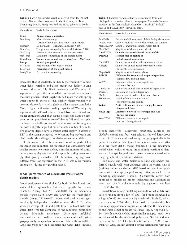
Table 3 Eleven bioclimatic variables derived from the PRISM

dataset. Five variables were used in the final analysis: Temp,TempRang, Precip, PrecipSeas and PcDryMo (shown in bold).

Abbreviation Variable description

Temp Annual mean temperature

DiurRang Mean diurnal range

(Mean of monthly (max temp – min temp))

Isotherm Isothermality ((DirRang/TempRang) * 100)

TempSeas Temperature seasonality (standard deviation * 100)

MaxTemp Maximum temperature of the warmest month

MinTemp Minimum temperature of the coldest month

TempRang Temperature annual range (MaxTemp – MinTemp)

Precip Annual precipitation

PcWetMo Precipitation of the wettest month

PcDryMo Precipitation of the driest month

PrecipSeas Precipitation seasonality

Journal of Biogeographyª 2015 John Wiley & Sons Ltd

6

T. E. Dilts et al.

correlation (r = 0.020 for bioclimatic and r = 0.055). Species

in which the mapped predictions differed the most tended to

occupy habitat along the Great Basin–Mojave Desert transi-

tional zone and the mapped differences clearly exhibited a

geographically clustered pattern (Fig. 4).

Relationship between shrub species and ecological

gradients

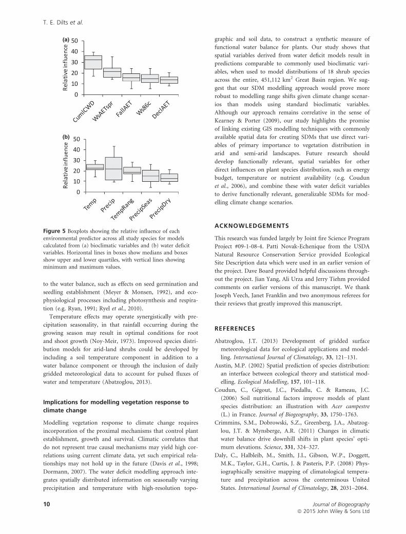
For models using the water deficit approach, the cumulative

water deficit variable was the most important predictor vari-

able with a mean relative influence of 31% compared to the

next highest variable (WsAETSpr), with a mean relative

influence of 22% (Fig. 5). Cumulative water deficit was the

most important predictor variable for 10 out of 18 species

with spring water supply (WsAETSpr) the most predictive

for five species, followed by monsoonality (Ws86c) for two

species, and fall AET for one species. In contrast, the biocli-

matic models showed less agreement in which variable was

selected as the most important. The top variable, tempera-

ture, had a mean relative influence of 24% which was only

slightly different from the next highest, precipitation, which

had a mean importance of 23%. The number of species in

which temperature was the best predictor was five, followed

by precipitation (five), temperature range (four), precipita-

tion seasonality (two), and precipitation in the driest month

(two).

Four of the five species that had spring water supply as

their most important water deficit predictor variable were

the montane species (mountain mahogany, mountain big

sagebrush, low sagebrush and antelope bitterbrush; see

Table 2 for their average elevation) with black greasewood

being the exception (Appendix S3). Fall AET was the most

predictive water deficit variable for winterfat. Broom snake-

weed and Mormon tea were best predicted by monsoonality,

which is reflected in their modelled distribution being

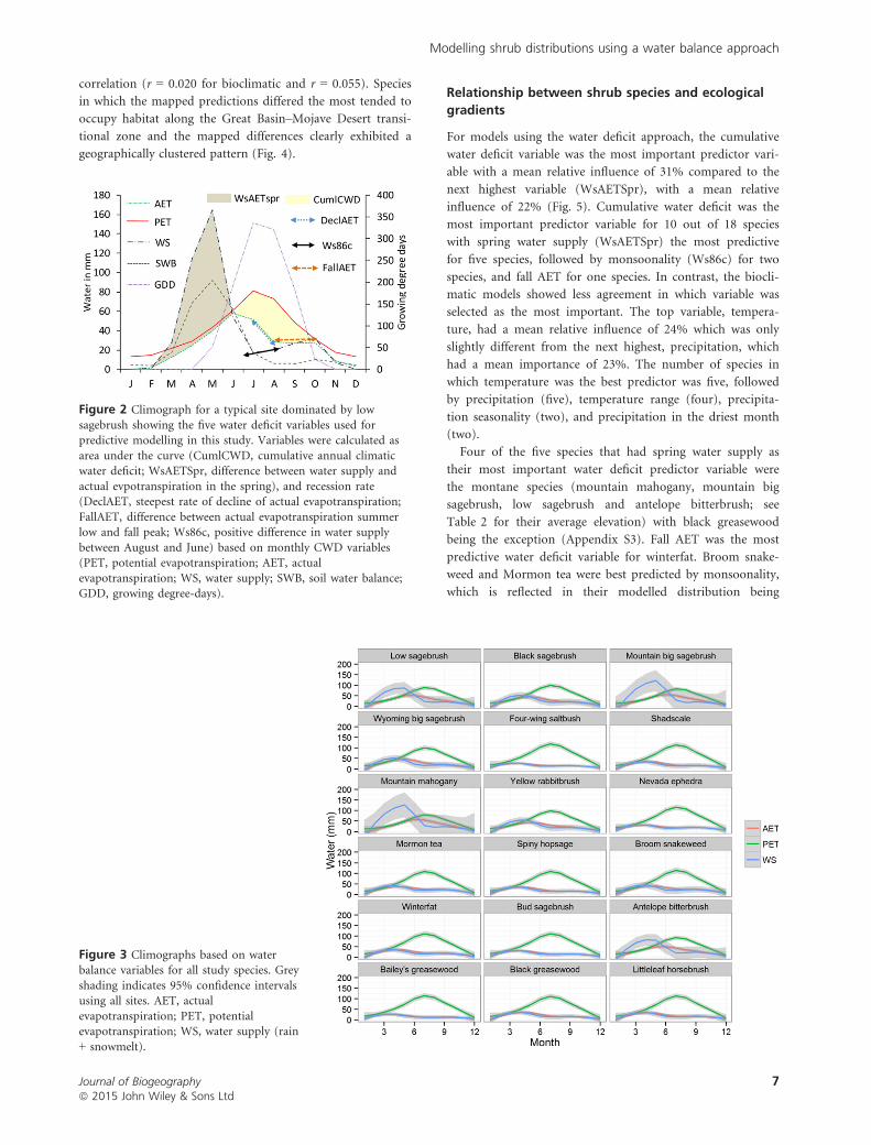
Figure 2 Climograph for a typical site dominated by low

sagebrush showing the five water deficit variables used forpredictive modelling in this study. Variables were calculated as

area under the curve (CumlCWD, cumulative annual climaticwater deficit; WsAETSpr, difference between water supply and

actual evpotranspiration in the spring), and recession rate(DeclAET, steepest rate of decline of actual evapotranspiration;

FallAET, difference between actual evapotranspiration summerlow and fall peak; Ws86c, positive difference in water supply

between August and June) based on monthly CWD variables(PET, potential evapotranspiration; AET, actual

evapotranspiration; WS, water supply; SWB, soil water balance;GDD, growing degree-days).

Figure 3 Climographs based on waterbalance variables for all study species. Grey

shading indicates 95% confidence intervalsusing all sites. AET, actual

evapotranspiration; PET, potentialevapotranspiration; WS, water supply (rain

+ snowmelt).

Journal of Biogeographyª 2015 John Wiley & Sons Ltd

7

Modelling shrub distributions using a water balance approach

centred in the south-east monsoonal portion of the study

area (Appendix S3).

Similarly, three of the five species that had precipitation as

their most predictive bioclimatic variable were montane spe-

cies (mountain mahogany, mountain big sagebrush and low

sagebrush) with bud sagebrush and four-wing saltbush being

exceptions (Appendix S3). Black greasewood, shadscale, win-

terfat and Mormon tea were best predicted by annual tem-

perature range. Broom snakeweed and littleleaf horsebrush

(Tetradymia glabrata) were best predicted by precipitation sea-

sonality, and yellow rabbitbrush (Chrysothamnus viscidiflorus)

and black sagebrush were best predicted by precipitation in the

driest month.

DISCUSSION

Does the water deficit approach yield better species

distribution models?

Correlative species distribution models have been criticized

for lacking mechanistic explanations and relying upon vari-

ables that are only indirectly related to plant resources, such

as water, light, and nutrients (Guisan & Zimmermann,

2000). Inferences regarding controls on species distributions

may be challenging to verify without recourse to experimen-

tation over such broad spatial scales, and can be difficult to

extrapolate to future climates. Species distribution models

have shown limited capacity to predict to new geographical

areas (Randin et al., 2006), and the lack of geographical

transferability may be due to overfit models (Heikkinen

et al., 2012) or environmental variables that correlate with,

but do not functionally influence, species distributions (Dor-

mann, 2007). Therefore, we expected that SDMs using water

deficit variables, which we considered to represent more

functional constraints upon species distribution, would prove

more generalizable.

Contrary to expectations, SDMs using variables con-

structed from a water deficit approach performed similarly

to SDMs using standard bioclimatic variables for predicting

arid-land shrub species distributions. Even when evaluating

low-elevation shrub species that are most water-limited, spe-

cies differences in predictive ability of the two modelling

approaches proved idiosyncratic (Table 5). Previous research

focused on tree species showed that water deficit approaches

resulted in improved predictions (Piedallu et al., 2013). We

ascribe the lack of improvement in model performance to

the ability of the bioclimatic variables to capture unique

aspects of the climate that the water deficit modelling did

not capture. In particular, temperature range and precipita-

tion seasonality appear to capture aspects of climate that are

not modelled very well by the water deficit approach. The

water deficit variables describing fall AET, rate of decline of

AET (DeclAET) and monsoonality (Ws86c) explained less of

the deviance compared to temperature range and precipita-

tion seasonality (Fig. 5).

Despite the lack of improved performance in model fit

and spatial transferability, the water deficit modelling

approach offers advantages over the bioclimatic approach in

that its predictor variables may be more interpretable than

standard bioclimatic variables, because they are more func-

tionally relevant and distinguish shrub species according to

key features of the seasonal water balance (Fig. 3). Interpre-

tation of simple climate variables, such as mean annual tem-

perature and precipitation, can be difficult because both

variables operate in tandem to influence site water balance.

Thus, use of predictor variables that serve as spatial proxies

for actual water resource limitation of arid-land shrub spe-

cies should result in improved capacity to explain changes in

species distributions in a warming environment (Franklin,

1995; Austin, 2002). However, the water balance approach

uses additional information on soils and topography that

may impart some additional error.

Dominant environmental influences on shrub species

distributions

Cumulative CWD was consistently selected as the most influ-

ential variable in our water deficit models. Other authors

have primarily used cumulative annual CWD and cumulative

annual AET for modelling plant distributions (Stephenson,

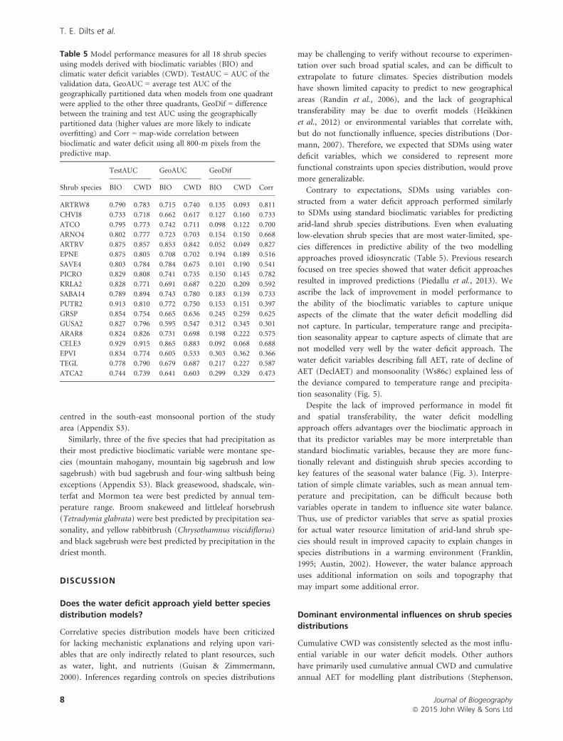
Table 5 Model performance measures for all 18 shrub species

using models derived with bioclimatic variables (BIO) andclimatic water deficit variables (CWD). TestAUC = AUC of the

validation data, GeoAUC = average test AUC of thegeographically partitioned data when models from one quadrant

were applied to the other three quadrants, GeoDif = differencebetween the training and test AUC using the geographically

partitioned data (higher values are more likely to indicateoverfitting) and Corr = map-wide correlation between

bioclimatic and water deficit using all 800-m pixels from thepredictive map.

Shrub species

TestAUC GeoAUC GeoDif

CorrBIO CWD BIO CWD BIO CWD

ARTRW8 0.790 0.783 0.715 0.740 0.135 0.093 0.811

CHVI8 0.733 0.718 0.662 0.617 0.127 0.160 0.733

ATCO 0.795 0.773 0.742 0.711 0.098 0.122 0.700

ARNO4 0.802 0.777 0.723 0.703 0.154 0.150 0.668

ARTRV 0.875 0.857 0.853 0.842 0.052 0.049 0.827

EPNE 0.875 0.805 0.708 0.702 0.194 0.189 0.516

SAVE4 0.803 0.784 0.784 0.675 0.101 0.190 0.541

PICRO 0.829 0.808 0.741 0.735 0.150 0.145 0.782

KRLA2 0.828 0.771 0.691 0.687 0.220 0.209 0.592

SABA14 0.789 0.894 0.743 0.780 0.183 0.139 0.733

PUTR2 0.913 0.810 0.772 0.750 0.153 0.151 0.397

GRSP 0.854 0.754 0.665 0.636 0.245 0.259 0.625

GUSA2 0.827 0.796 0.595 0.547 0.312 0.345 0.301

ARAR8 0.824 0.826 0.731 0.698 0.198 0.222 0.575

CELE3 0.929 0.915 0.865 0.883 0.092 0.068 0.688

EPVI 0.834 0.774 0.605 0.533 0.303 0.362 0.366

TEGL 0.778 0.790 0.679 0.687 0.217 0.227 0.587

ATCA2 0.744 0.739 0.641 0.603 0.299 0.329 0.473

Journal of Biogeographyª 2015 John Wiley & Sons Ltd

8

T. E. Dilts et al.

1990, 1998; Lutz et al., 2010; Piedallu et al., 2013). We

extended this previous approach by generating and further

analysing 18 additional variables derived from the CWD cli-

mograph, allowing a more synthetic description of how the

shape, rate and timing of the water balance change through

the year. We found several of these additional variables to be

important for predicting distribution of important shrub

types in the Great Basin, including difference between water

supply and actual evapotranspiration in spring (WsAETSpr),

difference between the minimum value of AET in summer

and the maximum value of AET in fall (FallAET), difference

between water supply in August and June (Ws86c), and the

steepest rate of decline in AET (DeclAET). In other systems

a wider range or different set of water deficit variables

may be useful for describing differences among plant

communities.

Relationships between water deficit variables and shrub

species distribution are consistent with results from detailed

ecohydrological modelling studies (Schlaepfer et al., 2012a)

that have linked sagebrush species occurrence to environ-

ments where spring recharge is followed by a dry period (i.e.

high WsAETSpr, high DeclAET). The spring water supply

variable (WsAETspr) is particularly important for modelling

the distribution of the more montane shrub species that

grow in areas where a large snowpack results in a large sur-

plus of soil water during the wet season followed by drying

during the summer growing season.

Previous studies have used water balance approaches

derived from CWD modelling to predict tree species distri-

butions (e.g. Lutz et al., 2010; Crimmins et al., 2011). Mech-

anistic process models have also been developed to quantify

the ecohydrological niche of sagebrush vegetation (Schlaepfer

et al., 2012a), and to create species distribution models for

big sagebrush (Schlaepfer et al., 2012b). Our results further

support the efficacy of water balance approaches, which

combine information on precipitation inputs, temperature-

related evapotranspiration outputs, and water holding

capacity of the soil, for defining the ecohydrological niche of

vegetation in water-limited landscapes. However, the ability

of bioclimatic models to predict as accurately or better than

water deficit models suggests that temperature has important

influences on shrub species distribution that may not relate

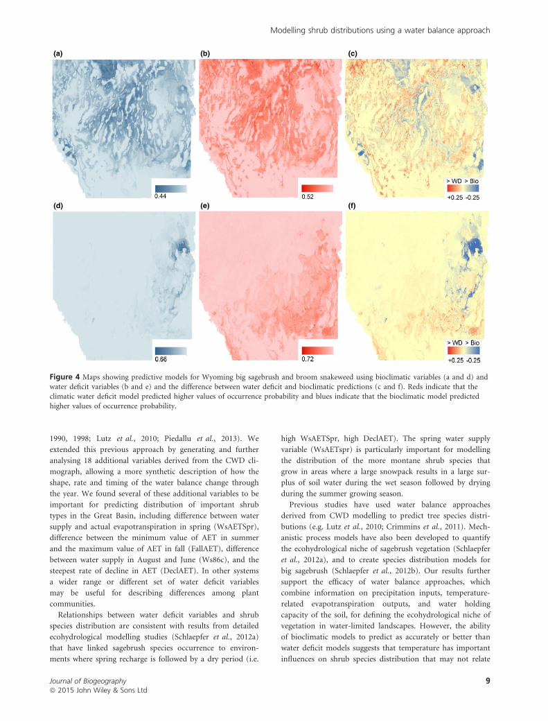
(a)

(d) (e) (f)

(b) (c)

Figure 4 Maps showing predictive models for Wyoming big sagebrush and broom snakeweed using bioclimatic variables (a and d) andwater deficit variables (b and e) and the difference between water deficit and bioclimatic predictions (c and f). Reds indicate that the

climatic water deficit model predicted higher values of occurrence probability and blues indicate that the bioclimatic model predictedhigher values of occurrence probability.

Journal of Biogeographyª 2015 John Wiley & Sons Ltd

9

Modelling shrub distributions using a water balance approach

to the water balance, such as effects on seed germination and

seedling establishment (Meyer & Monsen, 1992), and eco-

physiological processes including photosynthesis and respira-

tion (e.g. Ryan, 1991; Ryel et al., 2010).

Temperature effects may operate synergistically with pre-

cipitation seasonality, in that rainfall occurring during the

growing season may result in optimal conditions for root

and shoot growth (Noy-Meir, 1973). Improved species distri-

bution models for arid-land shrubs could be developed by

including a soil temperature component in addition to a

water balance component or through the inclusion of daily

gridded meteorological data to account for pulsed fluxes of

water and temperature (Abatzoglou, 2013).

Implications for modelling vegetation response to

climate change

Modelling vegetation response to climate change requires

incorporation of the proximal mechanisms that control plant

establishment, growth and survival. Climatic correlates that

do not represent true causal mechanisms may yield high cor-

relations using current climate data, yet such empirical rela-

tionships may not hold up in the future (Davis et al., 1998;

Dormann, 2007). The water deficit modelling approach inte-

grates spatially distributed information on seasonally varying

precipitation and temperature with high-resolution topo-

graphic and soil data, to construct a synthetic measure of

functional water balance for plants. Our study shows that

spatial variables derived from water deficit models result in

predictions comparable to commonly used bioclimatic vari-

ables, when used to model distributions of 18 shrub species

across the entire, 451,112 km2 Great Basin region. We sug-

gest that our SDM modelling approach would prove more

robust to modelling range shifts given climate change scenar-

ios than models using standard bioclimatic variables.

Although our approach remains correlative in the sense of

Kearney & Porter (2009), our study highlights the promise

of linking existing GIS modelling techniques with commonly

available spatial data for creating SDMs that use direct vari-

ables of primary importance to vegetation distribution in

arid and semi-arid landscapes. Future research should

develop functionally relevant, spatial variables for other

direct influences on plant species distribution, such as energy

budget, temperature or nutrient availability (e.g. Coudun

et al., 2006), and combine these with water deficit variables

to derive functionally relevant, generalizable SDMs for mod-

elling climate change scenarios.

ACKNOWLEDGEMENTS

This research was funded largely by Joint fire Science Program

Project #09-1-08-4. Patti Novak-Echenique from the USDA

Natural Resource Conservation Service provided Ecological

Site Description data which were used in an earlier version of

the project. Dave Board provided helpful discussions through-

out the project. Jian Yang, Ali Urza and Jerry Tiehm provided

comments on earlier versions of this manuscript. We thank

Joseph Veech, Janet Franklin and two anonymous referees for

their reviews that greatly improved this manuscript.

REFERENCES

Abatzoglou, J.T. (2013) Development of gridded surface

meteorological data for ecological applications and model-

ling. International Journal of Climatology, 33, 121–131.Austin, M.P. (2002) Spatial prediction of species distribution:

an interface between ecological theory and statistical mod-

elling. Ecological Modelling, 157, 101–118.Coudun, C., G�egout, J.C., Piedallu, C. & Rameau, J.C.

(2006) Soil nutritional factors improve models of plant

species distribution: an illustration with Acer campestre

(L.) in France. Journal of Biogeography, 33, 1750–1763.Crimmins, S.M., Dobrowski, S.Z., Greenberg, J.A., Abatzog-

lou, J.T. & Mynsberge, A.R. (2011) Changes in climatic

water balance drive downhill shifts in plant species’ opti-

mum elevations. Science, 331, 324–327.Daly, C., Halbleib, M., Smith, J.I., Gibson, W.P., Doggett,

M.K., Taylor, G.H., Curtis, J. & Pasteris, P.P. (2008) Phys-

iographically sensitive mapping of climatological tempera-

ture and precipitation across the conterminous United

States. International Journal of Climatology, 28, 2031–2064.

(a)

(b)

Figure 5 Boxplots showing the relative influence of each

environmental predictor across all study species for models

calculated from (a) bioclimatic variables and (b) water deficitvariables. Horizontal lines in boxes show medians and boxes

show upper and lower quartiles, with vertical lines showingminimum and maximum values.

Journal of Biogeographyª 2015 John Wiley & Sons Ltd

10

T. E. Dilts et al.

Das, A.J., Stephenson, N.L., Flint, A., Das, T. & van Mant-

gem, P.J. (2013) Climatic correlates of tree mortality in

water-and energy-limited forests. PLoS ONE, 8, e69917.

Davis, A.J., Jenkinson, L.S., Lawton, J.H., Shorrocks, B. &

Wood, S. (1998) Making mistakes when predicting shifts

in species range in response to global warming. Nature,

391, 783–786.Dilts, T.E. (2015) Climatic Water Deficit Toolbox for ArcGIS

10.1. Available at: http://www.arcgis.com/home/item.html?

id=de9ca57d43c041148b815da7ce4aa3a0

Dormann, C.F. (2007) Promising the future? Global change

projections of species distributions. Basic and Applied Ecol-

ogy, 8, 387–397.Dyer, J.M. (2009) Assessing topographic patterns in moisture

use and stress using a water balance approach. Landscape

Ecology, 24, 391–403.Elith, J., Leathwick, J.R. & Hastie, T. (2008) A working guide

to boosted regression trees. Journal of Animal Ecology, 77,

802–813.ESRI (2012) ArcGIS Desktop: Release 10.1. Environmental

Systems Research Institute, Redlands, CA.

Fielding, A.H. & Bell, J.F. (1997) A review of methods for

the assessment of prediction errors in conservation

presence/absence models. Environmental Conservation, 24,

38–49.Franklin, J. (1995) Predictive vegetation mapping: geographic

modelling of biospatial patterns in relation to environmen-

tal gradients. Progress in Physical Geography, 19, 474–499.Friedman, J.H. (2001) Greedy function approximation: a gra-

dient boosting machine. Annals of Statistics, 29, 1189–1232.Guisan, A. & Zimmermann, N.E. (2000) Predictive habitat

distribution models in ecology. Ecological Modelling, 135,

147–186.Heikkinen, R.K., Marmion, M. & Luoto, M. (2012) Does the

interpolation accuracy of species distribution models come

at the expense of transferability? Ecography, 35, 276–288.Hijmans, R.J. (2012) Cross-validation of species distribution

models: removing spatial sorting bias and calibration with

a null model. Ecology, 93, 679–688.Hijmans, R.J., Cameron, S.E., Parra, J.L., Jones, P.G. & Jarvis,

A. (2005) Very high resolution interpolated climate sur-

faces for global land areas. International Journal of Clima-

tology, 25, 1965–1978.Kearney, M. & Porter, W. (2009) Mechanistic niche model-

ling: combining physiological and spatial data to predict

species’ ranges. Ecology Letters, 12, 334–350.Lutz, J.A., van Wagtendonk, J.W. & Franklin, J.F. (2010) Cli-

matic water deficit, tree species ranges, and climate change

in Yosemite National Park. Journal of Biogeography, 37,

936–950.McCune, B. & Keon, D. (2002) Equations for potential

annual direct incident radiation and heat load. Journal of

Vegetation Science, 13, 603–606.Meyer, S.E. & Monsen, S.B. (1992) Big sagebrush germina-

tion patterns: subspecies and population differences. Jour-

nal of Range Management, 45, 87–93.

Miller, J. & Franklin, J. (2002) Modelling the distribution of

four vegetation alliances using generalized linear models

and classification trees with spatial dependence. Ecological

Modelling, 57, 227–247.Miller, J. & Franklin, J. (2006) Explicitly incorporating spa-

tial dependence in predictive vegetation models in the

form of explanatory variables: a Mojave Desert case study.

Journal of Geographical Systems, 8, 411–435.Noy-Meir, I. (1973) Desert ecosystems: environment and

producers. Annual Review of Ecology and Systematics, 4,

25–51.Omernik, J.M. (1987) Ecoregions of the conterminous Uni-

ted States. Annals of the Association of American Geogra-

phers, 77, 118–125.Paruelo, J.M. & Lauenroth, W.K. (1996) Relative abundance

of plant functional types in grasslands and shrublands of

North America. Ecological Applications, 6, 1212–1224.Piedallu, C., G�egout, J.C., Perez, V. & Lebourgeois, F. (2013)

Soil water balance performs better than climatic water

variables in tree species distribution modelling. Global

Ecology and Biogeography, 22, 470–482.PRISM Group. (2007) PRISM climatological normals, 1971–2000. The PRISM Group, Oregon State University, Corval-

lis, OR.

Radosavljevic, A. & Anderson, R.P. (2014) Making better

Maxent models of species distributions: complexity, over-

fitting and evaluation. Journal of Biogeography, 41, 629–643.

Randin, C.F., Dirnb€ock, T., Dullinger, S., Zimmermann,

N.E., Zappa, M. & Guisan, A. (2006) Are niche-based spe-

cies distribution models transferable in space? Journal of

Biogeography, 33, 1689–1703.Ridgeway, G. (2006) Generalized boosted regression models.

Documentation on the R package ‘gbm’, version 2.1.1.

Available at: http://cran.r-project.org/web/packages/gbm/

index.html.

Ryan, M.G. (1991) Effects of climate change on plant respi-

ration. Ecological Applications, 1, 157–167.Ryel, R.J., Leffler, A.J., Ivans, C., Peek, M.S. & Caldwel,

M.M. (2010) Functional differences in water use patterns

of contrasting life forms in Great Basin steppelands.

Vadose Zone Journal, 9, 548–560.Schlaepfer, D.R., Lauenroth, W.K. & Bradford, J.B. (2012a)

Effects of ecohydrological variables on current and future

ranges, local suitability patterns, and model accuracy in

big sagebrush. Ecography, 35, 374–384.Schlaepfer, D.R., Lauenroth, W.K. & Bradford, J.B. (2012b)

Ecohydrological niche of sagebrush ecosystems. Ecohydrol-

ogy, 5, 453–466.Stephenson, N.L. (1990) Climatic control of vegetation dis-

tribution: the role of the water balance. The American Nat-

uralist, 135, 649–670.Stephenson, N.L. (1998) Actual evapotranspiration and defi-

cit: biologically meaningful correlates of vegetation distri-

bution across spatial scales. Journal of Biogeography, 25,

855–870.

Journal of Biogeographyª 2015 John Wiley & Sons Ltd

11

Modelling shrub distributions using a water balance approach

U.S. Department of Agriculture (2009) Fire perimeter dataset,

monitoring trends in burn severity project. USDA Forest

Service/U.S. Geological Survey. Available at: http://

mtbs.gov/data/individualfiredata.html (accessed 23 March

2013).

U.S. Department of Agriculture (2013) Gridded Soil Survey Geo-

graphic (gSSURGO) Database for Nevada and Utah. United

States Department of Agriculture, Natural Resources Conser-

vation Service. Available at: http://datagateway.nrcs.usda.gov/

(accessed 23 March 2013).

U.S. Department of the Interior (2004a) U.S. Geological Sur-

vey National Gap Analysis Program, Southwest Regional

Gap Analysis Project Field Sample Database, version 1.1.

RS/GIS Laboratory, College of Natural Resources, Utah

State University, Logan, UT.

U.S. Department of the Interior (2004b) U.S. Geological Sur-

vey National Gap Analysis Program, Provisional Digital

Land Cover Map for the Southwestern United States, version

1.0. RS/GIS Laboratory, College of Natural Resources,

Utah State University, Logan, UT.

U.S. Department of the Interior (2008) Nevada fire history poly-

gons. U.S.D.I. Bureau of Land Management, Nevada State

Office. Available at: http://www.blm.gov/nv/st/en/prog/more_

programs/geographic_sciences/gis/geospatial_data.html

(accessed 23 March 2013).

West, N.E. (1983) Great Basin–Colorado Plateau sagebrush

semi-desert. Temperate deserts and semi-deserts (ed. by

N.E. West), pp. 331–349. Elsevier Science Publishers,

Amsterdam.

Whittaker, R.H. (1967) Gradient analysis of vegetation. Bio-

logical Reviews, 42, 207–264.

Whittaker, R.H. & Niering, W.A. (1965) Vegetation of the

Santa Catalina Mountains, Arizona: a gradient analysis of

the south slope. Ecology, 46, 429–452.

SUPPORTING INFORMATION

Additional Supporting Information may be found in the

online version of this article:

Appendix S1 Derivation of water deficit predictors and

maps showing the variables used in this study.

Appendix S2 Results of the principal components analysis

for bioclimatic and water deficit variables.

Appendix S3 Predictive maps and variable influence for

each species distribution model.

BIOSKETCH

Thomas Dilts is a research scientist in the Great Basin

Landscape Ecology Lab at the University of Nevada Reno.

His interests are in the application of geographic information

systems and remote sensing techniques for understanding

vegetation dynamics and for conservation planning.

All co-authors have interests in vegetation dynamics, climate

change, and ecosystem resilience and resistance to disturbance.

Author contributions: T.E.D., P.J.W. and J.C.C. conceived

the ideas; C.M.D. and T.E.D. analysed the data; and T.E.D.,

P.J.W. and J.C.C. led the writing.

Editor: Joseph Veech

Journal of Biogeographyª 2015 John Wiley & Sons Ltd

12

T. E. Dilts et al.