Functional methods for time series prediction: a

nonparametric approach

Germán Aneiros-Pérez�, Ricardo Caoyand Juan M.Vilar-Fernándezz

Departamento de Matemáticas

Facultad de Informática

Universidade da Coruña

Campus de Elviña, s/n

15071 A Coruña

Spain

Abstract

The problem of prediction in time series using nonparametric functional techniques

is considered. An extension of the local linear method to regression with functional

explanatory variable is proposed. This forecasting method is compared with the func-

tional Nadaraya-Watson method and with �nite-dimensional nonparametric predictors

for several real time series. Prediction intervals based on the bootstrap and conditional

distribution estimation for those nonparametric methods are compared too.

Keywords: Time series forecasting; Functional data; Nonparametric regression; Bootstrap

1 Introduction

Prediction of future observations is an important problem in time series. Given an observed

series Z1; Z2; : : : ; Zn, the aim is to predict a future value Zn+l, for some integer l � 1. A useful

�Corresponding author: E-mail: ganeiros@udc.es

yE-mail: rcao@udc.es

zE-mail: eijvilar@udc.es

1

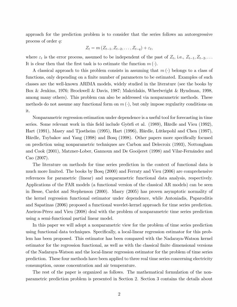
approach for the prediction problem is to consider that the series follows an autoregressive

process of order q:

Zt = m (Zt�1; Zt�2; : : : ; Zt�q) + "t;

where "t is the error process, assumed to be independent of the past of Zt, i.e., Zt�1; Zt�2; : : :

It is clear then that the �rst task is to estimate the function m (�).A classical approach to this problem consists in assuming that m (�) belongs to a class of

functions, only depending on a �nite number of parameters to be estimated. Examples of such

classes are the well-known ARIMA models, widely studied in the literature (see the books by

Box & Jenkins, 1976; Brockwell & Davis, 1987; Makridakis, Wheelwright & Hyndman, 1998,

among many others). This problem can also be addressed via nonparametric methods. These

methods do not assume any functional form on m (�), but only impose regularity conditions onit.

Nonparametric regression estimation under dependence is a useful tool for forecasting in time

series. Some relevant work in this �eld include Györ� et al. (1989), Härdle and Vieu (1992),

Hart (1991), Masry and Tjostheim (1995), Hart (1996), Härdle, Lütkepohl and Chen (1997),

Härdle, Tsybakov and Yang (1998) and Bosq (1998). Other papers more speci�cally focused

on prediction using nonparametric techniques are Carbon and Delecroix (1993), Nottongham

and Cook (2001), Matzner-Lober, Gannoun and De Gooijeret (1998) and Vilar-Fernández and

Cao (2007).

The literature on methods for time series prediction in the context of functional data is

much more limited. The books by Bosq (2000) and Ferraty and Vieu (2006) are comprehensive

references for parametric (linear) and nonparametric functional data analysis, respectively.

Applications of the FAR models (a functional version of the classical AR models) can be seen

in Besse, Cardot and Stephenson (2000). Masry (2005) has proven asymptotic normality of

the kernel regression functional estimator under dependence, while Antoniadis, Paparoditis

and Sapatinas (2006) proposed a functional wavelet-kernel approach for time series prediction.

Aneiros-Pérez and Vieu (2008) deal with the problem of nonparametric time series prediction

using a semi-functional partial linear model.

In this paper we will adopt a nonparametric view for the problem of time series prediction

using functional data techniques. Speci�cally, a local-linear regression estimator for this prob-

lem has been proposed. This estimator has been compared with the Nadaraya-Watson kernel

estimator for the regression functional, as well as with the classical �nite dimensional versions

of the Nadaraya-Watson and the local-linear regression estimator for the problem of time series

prediction. These four methods have been applied to three real time series concerning electricity

consumption, ozone concentration and air temperature.

The rest of the paper is organized as follows. The mathematical formulation of the non-

parametric prediction problem is presented in Section 2. Section 3 contains the details about

2

the local-linear regression estimator for functional data and how to use it to construct point

forecasts and nonparametric prediction intervals. A comparative empirical study of the new

method and other nonparametric approaches is included in Section 4, where some conclusions

are drawn.

2 Formulation of the problem

Let�s consider a continuous time stochastic process, fZ (t)gt2R, observed for t 2 [a; b), and

suppose we are interested in predicting Z (b+ r), for some r � 0. Let us assume that Z (t) is(or may be) stational, with seasonal length � and b = a+(n0 + 1) � . In other words, we assume

that the interval [a; b) consists of n0 + 1 seasonal periods of length � of the stochastic process

fZ (t)gt2R. For simplicity we will assume the following Markov property

Z (b+ r)jfZ(t);t2[a;b)gd= Z (b+ r)jfZ(t);t2[b��;b)g

By de�ning the functional data f(Xi; Yi)gn0

i=1, where Xi (t) = Z (a+ (i� 1) � + t) witht 2 C = [0; �), and Yi = Z (a+ i� + r) with r 2 C, we may look at the problem of predicting

Z (b+ r) by computing nonparametric estimations, m (xn0), of the autoregression functional:

m (xn0) = E�Y jX=xn0

�; (1)

with functional explanatory variable, X, and scalar response, Y .

In practice, typically we only observe a discrete version of the functional data in s equispaced

instants (s 2 N). More speci�cally, we only observe Xi (t) for t =js� , with j = 0; 1; : : : ; s� 1.

In such a case, de�ning n = (n0 + 1) s, we may formulate the prediction problem in terms of a

discrete-time process. Given the observed sample from the time series:

Z1 = Z (a) ; Z2 = Z

�a+

1

s�

�; : : : ;

Zn = Z

�a+

n0s+ s� 1s

�

�= Z

�b� 1

s�

�our aim is to predict

Zn+l = Z (b+ r) = Z

�a+

n0s+ s� 1 + ls

�

�;

with r = l�1s� , for some �xed l = 1; 2; : : : ; s.

3 Local-linear functional prediction

In the following we present the Nadaraya-Watson regression estimator for functional data and

extend it to the local linear estimator in the context of functional explanatory variable. These

3

two nonparametric estimators are useful techniques for point forecasting based on the autore-

gression functional.

Two methods are also introduced to compute prediction intervals based on the two previous

nonparametric forecasts. One is based on a bootstrap resampling of the residuals and the other

uses the conditional prediction distribution.

3.1 Nadaraya-Watson estimator for the regression functional

Given the functional sample f(Xi; Yi)gn0

i=1, the Nadaraya-Watson (NW) kernel estimator eval-

uated at a given function u, mh;NW (u), is of the form

mh;NW (u) =n0Xj=1

Wh;NW (u;Xj)Yj; (2)

where

Wh;NW (u;Xj) =Kh (kXj � uk)Pn0

i=1Kh (kXi � uk)with

Kh (t) =1

hK

�t

h

�being the rescaled kernel function with bandwidth h > 0 and k k being a suitable seminorm in

the functional space

F = ff : C �! R; f 2 L2g ;

and u 2 F (see Ferraty & Vieu, 2006, p. 55�56 and p. 223, for details on both the estimator (2)and the crucial role of the seminorm, respectively). The kernel K is a nonnegative real-valued

function such thatR10K (t) dt = 1.

3.2 Local-linear estimator for the regression functional

In this section we propose a local-linear (LL) functional regression estimator for (1) at u. We

extend the ideas in Fan and Gijbels (1996) to the case of functional data. First of all, we use

a linear approximation of m in a neighbourhood of a given function u:

m (x) ' �0 +ZC

� (t) (x (t)� u (t)) dt;

for some �0 2 R and � 2 F . The constant �0 plays the role of the value of m (u), while thefunction � is the gradient of m at the �point�u.

Given the sample f(Xi; Yi)gn0

i=1, de�ned above, we construct the LL estimator of �0 and �

as the minimizers of

(�0;�) =

n0Xi=1

�Yi �

��0 +

ZC

� (t) (Xi (t)� u (t)) dt��2

Kh;i; (3)

4

with Kh;i = Kh (kXi � uk), for a suitable seminorm k k.In order to minimize (3) with respect to �0 and �, we impose that the partial derivative

with respect to �0 is zero,

@

@�0= 0()

�0

n0Xi=1

Kh;i +n0Xi=1

Kh;i

ZC

� (t) (Xi (t)� u (t)) dt =n0Xi=1

Kh;iYi; (4)

and that the directional derivative of in the direction of any v 2 F is also zero,

@(�0;� + "v)

@"

����"=0

= 0()

�0

n0Xi=1

Kh;i

ZC

v (t) (Xi (t)� u (t)) dt

+n0Xi=1

Kh;i

�ZC

v (t) (Xi (t)� u (t)) dt��Z

C

� (t) (Xi (t)� u (t)) dt�

=n0Xi=1

Kh;iYi

�ZC

v (t) (Xi (t)� u (t)) dt�: (5)

In order to solve in �0 and � the system of functional equations (4) and (5) for all v 2 F , we�rst write the unknown function � in terms of a basis, fej (�)gj2N, of F , � (t) =

P1j=1 �jej (t),

and apply equation (5) for v = ek, k 2 N. Thus, we have the following in�nite dimensionalsystem of linear equations:

�0

n0Xi=1

Kh;i +1Xj=1

�j

n0Xi=1

Kh;iaij =n0Xi=1

Kh;iYi (6)

�0

n0Xi=1

Kh;iaik +1Xj=1

�j

n0Xi=1

Kh;iaijaik =n0Xi=1

Kh;iYiaik, k = 1; 2; : : : (7)

where

aij =

ZC

(Xi (t)� u (t)) ej (t) dt:

The system (6)-(7) can be written in a simpler way after introducing some new notation:

�0 = �0, bkj =n0Xi=1

Kh;iaikaij, for k; j 2 N;

b0j =

n0Xi=1

Kh;iaij, for j 2 N, bk0 =n0Xi=1

Kh;iaik, for k 2 N;

b00 =n0Xi=1

Kh;i, dk =n0Xi=1

Kh;iYiaik, for k 2 N, d0 =n0Xi=1

Kh;iYi:

5

This gives the following in�nite linear system:

1Xj=0

bkj�j = dk, k = 0; 1; : : : (8)

The solution of the previous system would give estimators of both m and the gradient

of m at u: mh;LL (u) = �0 = �0 and �h;LL (t) =P1

j=1 �jej (t), respectively. Of course, in

general is not possible to �nd an explicit solution of this in�nite dimensional linear system and

truncation ideas can be applied to solve a �nite dimensional approximation of (8). Fix some

N 2 N and consider just the �rst N +1 equations in (8). This requires �nding the solution ~�k,k = 0; 1; : : : ; N of

NXj=0

bkj�j = dk, k = 0; 1; : : : ; N:

Finally we obtain ~mh;N;LL (u) = ~�0 =~�0 and ~�h;N;LL (t) =

PNj=1~�jej (t). These are approxi-

mated solutions of (8), using only the �rst N functions in the basis: e1 (�), e2 (�), : : :, eN (�).

3.3 Residual-based bootstrap prediction intervals (RBB)

In this subsection and the next one, we follow the lines of Vilar-Fernández and Cao (2007). For

this reason we omit the details. The �rst bootstrap method for interval prediction is based on

resampling the residuals. A sketch of the algorithm follows.

1. Compute the residuals, "j = Yj � m (Xj), using some global cross-validation bandwidth,

where m (u) is either the NW or the LL estimator for functional data.

2. Use s", the standard deviation of the "j, to compute the smoothing parameter g =�43n0

�1=5s".

3. Draw smoothed bootstrap residuals

"�i = "Ii + g�i; i = 1; : : : ; B;

where Iid= U (f1; : : : ; n0g), �i

d= N (0; 1) and B is the number of bootstrap replications.

4. Sort the bootstrap residuals:�"�(i) : i = 1; : : : ; B

and compute the 1 � � prediction in-

terval: �m (Xn0) + "

�[(�=2)B]; m (Xn0) + "

�[(1�(�=2))B]

�:

6

3.4 Prediction intervals based on the conditional distribution (CD)

This method is based on estimating the conditional distribution function of Y jX=x. The ba-sic ideas can be found in Cao (1999). For a given real value y, the conditional cumulative

distribution function can be viewed as a regression function

F (yjx) = E�1fY�yg

��X=x

�:

Consequently, the functional NW or LL estimators can be used to estimate this conditional

distribution function. The prediction algorithm proceeds as follows.

1. Use the sample f(Xj; Yj) : 1 � j � n0g to compute F (yjx) using the NW or the LL

method. This function is smoothed again in the variable y.

2. The 1� � prediction interval is (L;U), where

F (LjXn0) =

�

2and F (U jXn0

) = 1� �2:

4 Comparative empirical study

The two functional data nonparametric point forecast and prediction intervals have been com-

pared with their �nite-dimensional counterparts. Speci�cally, these prediction methods have

been applied to three real time series concerning electricity consumption, ozone concentration

and air temperature. As we will show later, these time series are seasonal and, for each one, we

have 12 observations taken in equispaced instants within each seasonal period. In this sense,

we can consider that the length of the seasonal periods is � = 12 (in some units).

For the �nite-dimensional nonparametric approach we have followed the procedure in Vilar-

Fernández and Cao (2007). An important question in the �nite dimensional setting is how

to select the autoregressor variables, (Zt�i1 ; Zt�i2 ; : : : ; Zt�ip), for predicting Zt+l. We adopted

the approach by Tjostheim and Auestad (1994). It consists in minimizing a nonparametric

estimation of the �nal prediction error.

4.1 Selection of the tuning parameters

In the functional data setup (as well as in the �nite dimensional case) there are several tuning

parameters that need to be selected. We brie�y mention now the procedures that have been

used for this.

The Epanechnikov kernel has been used for the NW and the LL estimators. Cross-validation

methods (see Rachdi & Vieu, 2007; Benhenni et al., 2007), expressed in terms of k-nearest

neighbours, have been used for smoothing parameter selection. Global cross-validation is used

7

for constructing the residuals corresponding to the RBB prediction intervals, and local cross-

validation for computing the nonparametric point forecast and the estimation of the conditional

distribution function.

Following the recommendations of Ferraty and Vieu (2006, p. 223), for choosing the semi-

norm in practical situations we have based our choice on the smoothness or roughness of the

explanatory curves. Speci�cally, when the curves are smooth we have used the L2 norm of the

q-th derivative of the curve, k kderivativeq , while for rough curves the seminorm has been based on

principal component analysis, k kPCAq (q being the number of principal components). For the

de�nition of this class of seminorms see Ferraty and Vieu (2006, p. 28�30). The Fourier basis

was used in the LL functional estimator. The parameter q in the seminorm and the number of

functions in the Fourier basis, N , were also selected by cross-validation. The parameter N was

selected within f3; 5; 7g, while q was selected in the set f1; : : : ; 12g, when the seminorm is basedon principal components, and within f0; 1; 2g for the seminorm based on the q-th derivative.

When the prediction horizon is larger than one, point forecasts have been carried out in two

di¤erent ways. The �rst one is the direct method and consists in the approach mentioned in

the previous section. The second alternative is the recursive method. It computes a one-ahead

forecast and includes it in the sample to perform again a one-lag prediction, as many times as

needed. These two methods have been compared in the empirical study.

4.2 Methods and error criteria

Four nonparametric point forecasts are computed: (a) a �nite dimensional NW forecast, (b) a

�nite dimensional LL forecast, (c) a functional NW forecast and (d) a functional LL forecast.

These forecasts have been performed either using the direct method or the recursive one.

Four types of prediction intervals (only using the direct method) have been computed.

These are the four combinations for the nonparametric method used for point forecast (NW or

LL) and the basic procedure for constructing prediction intervals (residual based bootstrap and

conditional distribution). These four approaches have been used for both �nite dimensional

and functional autoregression estimation.

The nominal level for the prediction intervals was 95%. The number of bootstrap replications

was set to B = 1000. A maximum horizon of s = 12 was considered.

The performance of the point forecasts has been evaluated by excluding the last seasonal

period (last 12 observations) from the data, computing the point forecasts for these values and

comparing the predicted values, zn(l), with the real ones, zn+l. Several error measures have

been considered. The root mean squared error:

RMSE =

"1

s

sXl=1

(zn(l)� zn+l)2#1=2

;

8

the mean absolute error:

MAE =1

s

sXl=1

jzn(l)� zn+lj

and the relative error:

RE =1

s

sXl=1

jzn(l)� zn+lj�l

;

where �2l is the quasivariance of�z(j�1)�+l

n0j=1.

4.3 Electricity consumption data

The �rst data set analyzed consists of monthly electricity consumption in USA during the

period January 1972 �January 2005 (397 months). The data have been transformed using

logarithms and then di¤erentiated to eliminate the trend. The seasonal period for this time

series is one year. This gives 33 curves (see Ferraty and Vieu, 2006, p. 17�20, for details about

this data set). From Fig. 1 we can observe that the functional data are quite rough curves.

Thus we have used the class of seminormsnk kPCAq

o12q=1.

Table 1 collects the point forecasting errors, while Table 2 reports the tuning parameters

used.

Table 1

Error criteria for the �nite dimensional and functional

models using the Nadaraya-Watson (NW) and the

local-linear (LL) forecasts with the direct (D) and the

recursive (R) approach for the electricity consumption data

Error criteria

Estimator RMSE MAE RE

Finite dimensional

NW-D 0.0277 0.0225 0.7326

NW-R 0.0281 0.0224 0.7208

LL-D 0.0381 0.0321 1.0313

LL-R 0.0426 0.0357 1.1538

Functional

NW-D 0.0315 0.0260 0.8241

NW-R 0.0343 0.0287 0.9377

LL-D 0.0269 0.0218 0.6863

LL-R 0.0764 0.0470 1.7574

9

Table 2

Tuning parameters (q and N) for the Nadaraya-Watson (NW)

and the local-linear (LL) forecast using the direct (D) and the

recursive (R) approach for the electricity consumption data

Prediction horizon

Estimator 1 2 3 4 5 6 7 8 9 10 11 12

NW-D: q 8 1 2 7 1 3 1 5 12 3 1 7

NW-R: q 8 12 4 6 2 1 5 6 12 1 3 7

LL-D: q 5 1 3 12 12 5 1 1 5 1 1 1

LL-R: q 5 2 11 10 1 3 3 12 1 1 12 2

LL-D: N 3 3 5 3 3 5 3 7 3 5 5 5

LL-R: N 3 3 3 3 3 5 3 3 3 3 3 3

Fig. 1 shows some plots of the time series along time, the functional data and the best

forecasts, for every type of model and estimator. In other words, for each kind of model

(�nite dimensional or functional) and each kind of estimator (NW or LL), only the results

corresponding to the best (direct or recursive) forecast are shown. Fig. 2 reports the prediction

intervals (only using the direct method) for the four nonparametric forecasts (NW and LL

either �nite dimensional or functional) with the two possible methods for interval construction

(RBB and CD).

10

Fig. 1. Time series and functional data (upper panels) together with the best forecasted

(di¤erenced log) electricity consumption for each type of model and estimator (lower panels).

Both the direct (D) and the recursive (R) method were combined with both the Nadaraya-

Watson (NW) and the local-linear (LL) estimator.

11

Fig. 2. Prediction intervals corresponding to the (di¤erenced log) electricity consumption data.

They are based on both �nite dimensional (upper panels) and functional (lower panels) models.

The Nadaraya-Watson (NW) and the local-linear (LL) estimator were used for constructing the

residual-based bootstrap (RBB) prediction intervals and the prediction intervals based on the

conditional distribution (CD). Only the direct (D) method was considered.

4.4 Ozone concentration data

The second series collects ozone concentrations every second hour from May 18, 2005 to June

29, 2005 (516 data) recorded in Getafe (Madrid, Spain). There exist a clear daily seasonality

in this series, which gives 43 curves (see Aneiros-Pérez and Vieu, 2008, for more information

about this series). The smooth shape of the curves (see Fig. 3) suggests to use the class of

seminormsnk kderivativeq

o2q=0.

12

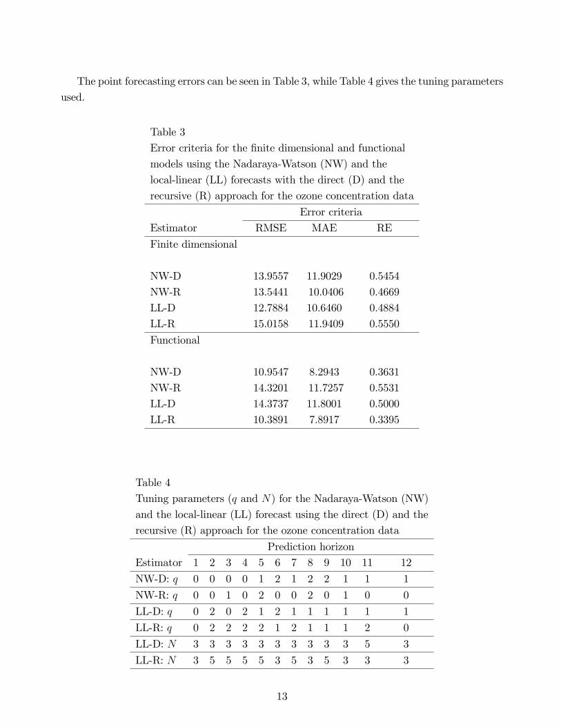
The point forecasting errors can be seen in Table 3, while Table 4 gives the tuning parameters

used.

Table 3

Error criteria for the �nite dimensional and functional

models using the Nadaraya-Watson (NW) and the

local-linear (LL) forecasts with the direct (D) and the

recursive (R) approach for the ozone concentration data

Error criteria

Estimator RMSE MAE RE

Finite dimensional

NW-D 13.9557 11.9029 0.5454

NW-R 13.5441 10.0406 0.4669

LL-D 12.7884 10.6460 0.4884

LL-R 15.0158 11.9409 0.5550

Functional

NW-D 10.9547 8.2943 0.3631

NW-R 14.3201 11.7257 0.5531

LL-D 14.3737 11.8001 0.5000

LL-R 10.3891 7.8917 0.3395

Table 4

Tuning parameters (q and N) for the Nadaraya-Watson (NW)

and the local-linear (LL) forecast using the direct (D) and the

recursive (R) approach for the ozone concentration data

Prediction horizon

Estimator 1 2 3 4 5 6 7 8 9 10 11 12

NW-D: q 0 0 0 0 1 2 1 2 2 1 1 1

NW-R: q 0 0 1 0 2 0 0 2 0 1 0 0

LL-D: q 0 2 0 2 1 2 1 1 1 1 1 1

LL-R: q 0 2 2 2 2 1 2 1 1 1 2 0

LL-D: N 3 3 3 3 3 3 3 3 3 3 5 3

LL-R: N 3 5 5 5 5 3 5 3 5 3 3 3

13

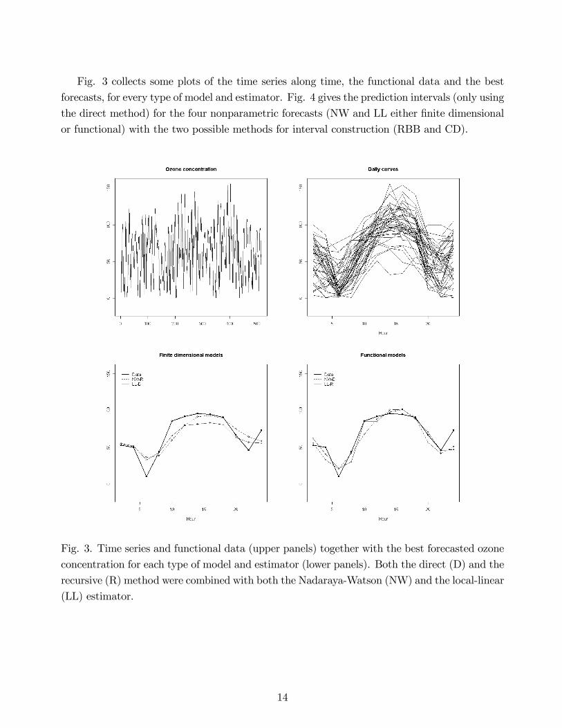
Fig. 3 collects some plots of the time series along time, the functional data and the best

forecasts, for every type of model and estimator. Fig. 4 gives the prediction intervals (only using

the direct method) for the four nonparametric forecasts (NW and LL either �nite dimensional

or functional) with the two possible methods for interval construction (RBB and CD).

Fig. 3. Time series and functional data (upper panels) together with the best forecasted ozone

concentration for each type of model and estimator (lower panels). Both the direct (D) and the

recursive (R) method were combined with both the Nadaraya-Watson (NW) and the local-linear

(LL) estimator.

14

Fig. 4. Prediction intervals corresponding to the ozone concentration data. They are based on

both �nite dimensional (upper panels) and functional (lower panels) models. The Nadaraya-

Watson (NW) and the local-linear (LL) estimator were used for constructing the residual-based

bootstrap (RBB) prediction intervals and the prediction intervals based on the conditional

distribution (CD). Only the direct (D) method was considered.

4.5 Air temperature data

The Mabegondo data is the third time series we will analyze. Air temperature has been recorded

every two hours at Mabegondo meteorologic station (Mabegondo, Galicia, Spain) over the

period January 1st 2008 �March 30th 2008. The seasonal period is one day (1092 data and

91 curves). As in the case of the ozone concentration data, we are in a situation in which the

curves are smooth (see Fig. 5). Thus we have used the class of seminormsnk kderivativeq

o2q=0.

15

Table 5 reports the point forecasting errors, while Table 6 shows the tuning parameters

used.

Table 5

Error criteria for the �nite dimensional and functional

models using the Nadaraya-Watson (NW) and the

local-linear (LL) forecasts with the direct (D) and the

recursive (R) approach for the air temperature data

Error criteria

Estimator RMSE MAE RE

Finite dimensional

NW-D 3.4198 3.0401 1.0730

NW-R 3.8345 3.3167 1.1674

LL-D 3.3392 2.9590 1.0516

LL-R 3.2507 2.8530 0.9827

Functional

NW-D 2.8224 2.5496 0.8886

NW-R 2.5482 2.2725 0.7891

LL-D 2.0530 1.8415 0.6556

LL-R 2.4964 1.9118 0.6658

Table 6

Tuning parameters (q and N) for the Nadaraya-Watson (NW)

and the local-linear (LL) forecast using the direct (D) and the

recursive (R) approach for the air temperature data

Prediction horizon

Estimator 1 2 3 4 5 6 7 8 9 10 11 12

NW-D: q 0 0 0 0 0 0 0 0 0 0 0 0

NW-R: q 0 0 0 0 0 0 0 0 0 0 0 0

LL-D: q 1 0 0 0 0 2 2 2 0 1 1 1

LL-R: q 1 0 0 2 2 0 0 0 2 0 0 1

LL-D: N 3 5 5 5 5 5 5 5 3 3 3 3

LL-R: N 3 5 5 5 5 5 5 5 5 5 7 7

16

Fig. 5 shows some plots of the time series along time, the functional data and the best

forecasts, for every type of model and estimator. Fig. 6 gives the prediction intervals (only using

the direct method) for the four nonparametric forecasts (NW and LL either �nite dimensional

or functional) with the two possible methods for interval construction (RBB and CD).

Fig. 5. Time series and functional data (upper panels) together with the best forecasted air

temperature for each type of model and estimator (lower panels). Both the direct (D) and the

recursive (R) method were combined with both the Nadaraya-Watson (NW) and the local-linear

(LL) estimator.

17

Fig. 6. Prediction intervals corresponding to the air temperature data. They are based on

both �nite dimensional (upper panels) and functional (lower panels) models. The Nadaraya-

Watson (NW) and the local-linear (LL) estimator were used for constructing the residual-based

bootstrap (RBB) prediction intervals and the prediction intervals based on the conditional

distribution (CD). Only the direct (D) method was considered.

4.6 Some comments on the empirical results

Some interesting facts can be seen in Figs. 1, 3 and 5. First, we observe that the curves corre-

sponding to the electricity data are rough while those corresponding to both ozone concentration

and air temperature data are smooth. Second, we note that the curves corresponding to the

last two data sets are more sparse than those corresponding to the electricity data. Thus, this

study covers di¤erent and interesting situations in practice. Finally, from a graphical point of

view, these �gures suggest that (except perhaps for the case of the �nite dimensional predictors

18

applied to the air temperature data) the nonparametric forecasts show a good behavior, in the

sense that the predictions follow the trend of the data.

To compare quantitatively the di¤erent prediction methods used in this paper, we need to

consider the information contained in the Tables 1, 3 and 5. On the one hand, these tables

show that the LL forecast for functional data (most of the time the direct version) beats the

other nonparametric methods (either �nite dimensional or functional) for the analyzed series.

On the other hand, we should mention the problems in the use of the recursive method, because

a poor prediction in an speci�c instant causes even worse predictions for the instants later.

Figs. 2, 4 and 6 report results on the prediction intervals. From these �gures, and focusing

in each class of models (�nite dimensional or functional models), there are no large di¤erences

between the intervals constructed by NW estimators and those constructed using LL. Never-

theless, prediction intervals using the functional data approach are, generally speaking, more

narrow than those using �nite dimensional models. In addition, functional LL-RBB prediction

intervals are most of the time more accurate and narrow than the others.

5 References

Aneiros-Pérez, G. & Vieu, P. (2008). Nonparametric time series prediction: A semi-functional

partial linear modeling. Journal of Multivariate Analysis, 99, 834-857.

Antoniadis, A., Paparoditis, E. & Sapatinas, T. (2006). A functional wavelet-kernel approach

for time series prediction. Journal of the Royal Statistical Society, Series B, 68, 837-857.

Benhenni, K., Ferraty, F., Rachdi, M. & Vieu, P. (2007). Local smoothing regression with

functional data. Computational Statistics, 22, 353-369.

Besse, P. C., Cardot, H. & Stephenson, D. B. (2000). Autoregressive forecasting of some

functional climatic variations. Scandinavian Journal of Statistics, 27, 673-687.

Bosq, D. (1998). Nonparametric Statistics for Stochastic Processes: Estimation and Prediction,

Lecture Notes in Statistics, 110. Springer.

Bosq, D. (2000). Linear Processes in Function Spaces: Theory and Applications, Lecture Notes

in Statistics, 149. Springer.

Box, G. E. P & Jenkins, G. M. (1976). Time Series Analysis: Forecasting and Control. Holden-

Day.

Brockwell, P. J. & Davis, R. A. (1987). Time series: Theory and methods. Springer.

Cao, R. (1999). An overview of bootstrap methods for estimating and predicting in time series.

Test, 8, 95-116.

Carbon, M. & Delecroix, M. (1993). Non-parametric vs parametric forecasting in time series:

a computational point of view. Applied Stochastic Models and Data Analysis, 9, 215-229.

Fan, J. & Gijbels, I. (1996). Local Polynomial Modelling and its Applications. Chapman and

19

Hall.

Ferraty, F. & Vieu, P. (2006). Nonparametric Functional Data Analysis, Springer Series in

Statistics. New York: Springer-Verlag.

Györ�, L., Härdle, W., Sarda, P. & Vieu, P. (1989). Nonparametric Curve Estimation from

Time Series, Lecture Notes in Statistics, 60. Springer.

Härdle, W., Lütkepohl, H. & Chen, R. (1997). A review of nonparametric time series analysis.

International Statistical Review, 65, 49-72.

Härdle, W., Tsybakov, A. & Yang, L. (1998). Nonparametric vector autoregression. Journal of

Statistical Planning and Inference, 68, 22-245.

Härdle, W. & Vieu, P. (1992). Kernel regression smoothing of time series. Journal of the Time

Series Analysis, 13, 209-232.

Hart, J. D. (1991). Kernel regression estimation with time series errors. Journal of the Royal

Statistical Society, Series B, 53, 173-187.

Hart, J. D. (1996). Some automated methods of smoothing time-dependent data. Journal of

Nonparametric Statistics, 6, 115-142.

Makridakis, S., Wheelwright, S. C. & Hyndman, R. J. (1998). Forecasting: Methods and

Applications. Wiley.

Masry, E. (2005). Nonparametric regression estimation for dependent functional data: asymp-

totic normality. Stochastic Processes and their Applications, 115, 155-177.

Masry, E. & Tjostheim, D. (1995). Nonparametric estimation and identi�cation of nonlinear

ARCH time series. Econometric Theory, 11, 258-289.

Matzner-Lober, E., Gannoun, A. & De Gooijer, J. G. (1998). Nonparametric forecasting: a

comparison of three kernel based methods. Communications in Statistics: Theory and Methods,

27, 1593-1617.

Nottongham, Q. J. & Cook, D. C. (2001). Local linear regression for estimating time series

data. Computational Statistics and Data Analysis, 37, 209-217.

Rachdi, M. & Vieu, P. (2007). Nonparametric regression for functional data: Automatic

smoothing parameter selection. Journal of Statistical Planning and Inference, 137, 2784-2801.

Tjostheim, D. & Auestad, B. H. (1994). Nonparametric identi�cation of nonlinear time series:

selecting signi�cant lags. Journal of the American Statistical Association, 89, 1410-1419.

Vilar-Fernández, J.M. & Cao, R. (2007). Nonparametric forecasting in time series �A com-

parative study. Communications in Statistics: Simulation and Computation, 36, 311-334.

20